Embed Size (px)
Citation preview

Analysis of the Dual Problem of the Weighted RASMethod: Castilla–La Mancha application
F. Escobedo1 2, R. Mınguez3 and J. M. Urena4
Abstract
This paper uses a variant of RAS Method in which weights are attached tothe percentage changes in the input-output cell values. In this way the weightedRAS dual problem, associated to the primal optimization problem, is solved andinterpreted from a sensitivity point of view. It is found that the optimum values ofthe dual variables are dependent on the restriction taken out from the initial onesto fulfill the condition for compatibility, that is, the sum of columns has to be equalto the sum of rows. For this reason a method has been developed to attain a newdual sensitivity matrix whose elements are not affected by the restriction is takenout. Finally this theoretical analysis is used to update the Input-Output Tables ofCastilla-La Mancha 1995.
Key Words: RAS Method, Sensitivity Analysis, Duality, Weighting Techniques, Re-
gional Development, Castilla–La Mancha.
1 Introduction
Sensitivity analysis consists of determining “how” and “how much” specific changes in
the parameters of an optimization problem influence the optimal objective function value
and the point (or points) where the optimum is attained.
The problem of sensitivity analysis in nonlinear programming has been discussed by
several authors, as, for example, Vanderplaats [20], Sobiesky et al. [18], Enevoldsen, [11],
Roos, Terlaky and Vial [17], Bjerager and Krend [3], etc. There are at least three ways
of deriving equations for the unknown sensitivities: (a) the Lagrange multiplier equations
of the constrained optimum (see Sobiesky et al. [18]), (b) differentiation of the Karush–
Kuhn–Tucker conditions to obtain the sensitivities of the objective function with respect
1Current address: Faculty of Economics, University of Groningen, PO Box 800, 9700 AV Groningen,The Netherlands. [email protected]. Tel: + 31 50 363 3720. Permanent address: School of CivilEngineering, University of Castilla-La Mancha, Avenida de Camilo Jose Cela 2, 13071 Ciudad Real,Spain. [email protected]. Tel: 926 295 300
2The author wants to emphasize his thankfulness to Dr. Jan Oosterhaven for his comments andsuggestions to improve the quality and accuracy of the research undertaken.
3School of Civil Engineering, University of Castilla-La Mancha, Avenida de Camilo Jose Cela 2, 13071Ciudad Real, Spain. [email protected]. Tel: 926 295 300
4School of Civil Engineering, University of Cantabria, Avenida de Los Castros s/n, 39005 Santander,Spain. [email protected]. Tel: 942 201 711
1

to changes in the parameters (see Vanderplaats [20], Sorensen and Enevoldsen [19] or
Enevoldsen, [11]), and (c) the extreme conditions of a penalty function (see Sobiesky et
al. [18]).
The existing methods for sensitivity analysis may present four main limitations:
1. They provide the sensitivities of the objective function value and the primal variables
values with respect to parameters, but not the sensitivities of the dual variables with
respect to parameters.
2. For different cases there are diverse methods for obtaining each of the sensitivities
(optimal objective function value or primal variable values with respect to parame-
ters), but there is no integrated approach providing all the sensitivities at once.
3. They assume the existence of partial derivatives of the objective function or the
optimal solutions with respect to the parameters; however, this is not always the
case. In fact, there are cases in which partial or directional derivatives fail to exist.
In addition, most techniques reported in the literature do not distinguish between
right and left derivatives. Ross, Terlaky and Vial [17] state:
“It is surprising that in the literature on sensitivity analysis it is far from
common to distinguish between left- and right-shadow prices”.
By left- and right-shadow prices they mean left- and right-derivatives of the objective
function with respect to parameters at the current optimal value.
4. They assume that the active constraints remain active, which implies that there is
no need to distinguish between equality or inequality constraints, because all the
active constraints can be considered as equality constraints, and inactive constraints
will remain inactive for small changes in the parameters. As a consequence, the set
of possible changes (perturbations) has (locally) the structure of a linear space.
2 Methodology
In this section we analyze the sensitivity of the optimal solution of a nonlinear program-
ming problem to changes in the data values. Many authors, as those already mentioned,
have studied different versions of this problem. Some of them have dealt with the linear
programming problem and discussed the effect of changes of (i) the cost coefficients, (ii)
the right hand sides of the constraints or (iii) the constraint coefficients on either (a) the
2

optimal value of the objective function or (b) the optimal solution. A similar analysis has
been done for nonlinear problems. However, these authors have dealt only with changes
that keep invariant the set of active constraints.
The goal consists in getting a interindustry transactions matxix z as close as posible
to the original one zo, using a special measurement between matrixes. It is rather logical,
if we do not have more detailed information, to modify as less as possible the economic
structure [13].
Consider the following Nonlinear Programming Problem (NLPP) [1] and [14]:
Minimizez
f(z, zo, w) =m∑
i=1
∑∀j; (i,j)/∈Ω0
zij ln
(wij
zij
zoij
), (1)
subject tom∑
j=1
zij = ui; i = 1, . . . ,m, : λi (2)
m∑i=1
zij = vj; i = 2, . . . ,m : µj, (3)
where w is the vector which contains the associated weights to each transfer, u and v are
the sum by rows and columns of the final interindustry transactions matxix, respectively,
and the set Ω0 contains the indexes of the zero-elements of the matrix zo; the use of this
set is due to the fact that the objective function is not defined for those specific values.
This involves that once the problem is solved (1)-(3) the elements of the new matrix whose
indexes agreed with those of Ω0 set are zero zij = 0; ∀(i, j) ∈ Ω0. In this way it could be
added an aditional restriction to the original problem that would not change the solution:
zi,j = zoij; ∀(i, j) ∈ Ω0 : κij. (4)
All the depicted elements so far belong to the primal problem. On the other hand it is
known that any optimization problem has another problem very linked to it named dual
problem, where λ, µ and κ are their variables (dual variables), which are associated to
the restrictions of primal problem (2)-(4), respectively.
We should note that the solution of the problem (1)-(4) has to fulfil the following
condition:
m∑i=1
ui =m∑
j=1
vj, (5)
For that reason the number of restrictions is 2m − 1, that is, one of the restrictions
has been eliminated to keep always the condition of compatibility. Later it is explained
3

why it has been chosen to eliminate the sum of the first column and what is the effect if
another restriction is eliminated.
The dual problem of primal problem (1)-(4) in this situation is defined as:
Maximizeλ, µ, κ
φ(λ, µ, κ) , (6)
where the function φ is the dual function.
Using the Lagrangian function:
L(z, λ, µ) = f(z, zo, w) + λTh(z, u) + µT g(z, v) + κT t(z, zo), (7)
where z is the vector of the decision variables, f : IRm2−nz → IR is the objective function,
and h : IRm → IRm, g : IRm → IRm−1 and t : IRnz → IRnz , where nz is the number of
elements of set Ω0, and h(z, u), g(z, v) and t(z, zo) are the equality restraints linked to
the sum by rows (2), to the sum by columns (3) and the null elements (4), respectively.
The dual problem (6) can be rewritten as:
maximizeλ, µ, κ
Infimumz
L(z, zo, w, u, v, λ, µ, κ)
(8)
Remark 1 It is supposed that f, h, g, and t are in such way that the infimum of la-
grangian function is reached in some point z, in such way that the infimum operator in
(8) can be replaced with the minimum operator. For this reason the problem (8) is known
as dual problem max–min.
The lagrangian function particularized for the problem (2)-(4) is:
L(z, zo, w, u, v, λ, µ, κ) =m∑
i=1
∑∀j; (i,j)/∈Ω0
zij ln
(wij
zij
zoij
)+
m∑i=1
λi
m∑j=1
zij − ui
+
m∑j=2
µj
(m∑
i=1
zij − vj
)+
∑∀(i,j)∈Ω0
κij
(zij − zo
ij
).
(9)
Definition 1 (Regular point). The solution to an optimization problem z∗, λ∗, µ∗,
κ∗ and f ∗ is considered a regular point if the active restrictions gradients are linearly
independient.
4

Theorem 1 (Sensitivities with respect to the objetive function). If we have the
optimization problem (1)-(4) whose solution is a regular point, then it is carried out that:
∂f(z∗, zo, w)
∂ui
= −λi; i = 1, . . . ,m, (10)
∂f(z∗, zo, w)
∂vj
= −µj; i = 2, . . . ,m, (11)
∂f(z∗, zo, w)
∂aij
= −κij; ∀(i, j) ∈ Ω0, (12)
that is, the sensitivities of the optimum value of the problem objective function (1)-(4)
with respect to the changes in the parameters u, v and the null terms of zo, that are in
the right terms of the restrictions (2)-(4), respectively, agreed with the optimum values of
the dual variables associated to each restriction with the opposite sign.
The demonstration of this theorem can be found, for example, in Luenberger [12] or
Conejo et al. [10].
It is important to insist that the parameters whose sensitivities we want to know have
to appear in the right terms of the restrictions for this theorem to be applied. For that
reason, it is not possible with this method to know the sensitivity of the objective function
with respect to the weights w and the non null terms of the initial matrix zo.
Now the starting point is the non-linear equations system but including the dual
variables associated to all the sums by rows and by columns, that is, we take out the
condition ∀j/ j ≥ 2. If the terms are reorganized we have the following linear equations
system:
λi + µj = −1− ln
(wij
zij
zoij
); i = 1; . . . , m; ∀j/ (i, j) /∈ Ω0 (13)
λi + µj + κij = 0; ∀(i, j) ∈ Ω0. (14)
First of all we focus on (13) which allow us to calculate the multipliers λ and µ, and
later we will get the values of κ using (14).
We have in (13) m2−nz equations while the number of unknowns is 2m if we take into
account that we include the associated multipliers to every sum by rows and by columns
and that the condition of compatibility (5) is kept.
As it can be seen in normal conditions, that is, if the number of null elements in the
original matriz zo fulfils that nz ≤ m2−2m, then we have enough number of equations to
solve the system (13). In fact, in the majority of the cases we have more equations than
5

the necessary ones; in that case we have to select the system coefficients matrix (13), that
is going to be called cλ,µ, sub-matrix whose rank is equal to 2m, and proceed to solve.
The starting point for the suitable selection of that coefficients sub-matrix is the
original coefficients matrix.
In principle it is considered that there are not null elements in the original matrix zo,
that is, nz = 0 to simplify the analysis. In this case the structure of coefficients matrix
cλ,µ and the independent terms vector bλ,µ is:
cλ,µ =
λ1 0 0 · · · 0 µ1 0 0 · · · 0λ1 0 0 · · · 0 0 µ2 0 · · · 0...
......
. . ....
......
.... . .
...λ1 0 0 · · · 0 0 0 0 · · · µm
0 λ2 0 · · · 0 µ1 0 0 · · · 00 λ2 0 · · · 0 0 µ2 0 · · · 0...
......
. . ....
......
.... . .
...0 λ2 0 · · · 0 0 0 0 · · · µm
0 0 λ3 · · · 0 µ1 0 0 · · · 00 0 λ3 · · · 0 0 µ2 0 · · · 0...
......
. . ....
......
.... . .
...0 0 λ3 · · · 0 0 0 0 · · · µm
......
.... . .
......
......
. . ....
0 0 0 · · · λm µ1 0 0 · · · 00 0 0 · · · λm 0 µ2 0 · · · 0...
......
. . ....
......
.... . .
...0 0 0 · · · λm 0 0 0 · · · µm
and bλ,µ =
−1− ln (w11z11/zo11)
−1− ln (w12z12/zo12)
...−1− ln (w1mz1m/zo
1m)−1− ln (w21z21/z
o21)
−1− ln (w22z22/zo22)
...−1− ln (w2mz2m/zo
2m)−1− ln (w31z31/z
o31)
−1− ln (w32z32/zo32)
...−1− ln (w3mz3m/zo
3m)...
−1− ln (wm1zm1/zom1)
−1− ln (wm2zm2/zom2)
...−1− ln (wmmzmm/zo
mm)
.
(15)
Using the ortogonalization method proposed by Castillo et al. [4, 5, 8], it can be
demonstrated that the coefficients matrix rank cλ,µ is 2m− 1; therefore the solution of
the system (13) is a vectorial space (see Padberg [15] and Castillo et al. [6, 7]) in the
following way:
[λµ
]=
[λ0
µ0
]+ ρ
[λ1
µ1
], (16)
composed by a particular solution (λ0, µ0)T plus a vectorial space where ρ ∈ IR, and
(λ1, µ1)T are the solution of the homogeneous space.
As ρ can take infinite values, the system, and therefore the dual problem, has infinite
solutions. For that reason in the primal problem (1)-(4) it is eliminated the restriction
6

associated to the first row; in that way the linear system needed to solve the dual problem
has 2m− 1 rank, so the number of equations 2m− 1 is equal to the number of unknowns
2m− 1 and the system has an unique solution.
Remark 2 It is necessary to eliminate one of the equations sum by rows or sum by
columns for the system (13) and therefore the dual problem has a unique solution. This is
due to one of the equations means redundant information for the compatibility condition
(5).
In the Figure 1 it is shown a graphic interpretation of the effect of a redundant restraint
in the solution of an optimization problem. It has to be underlined that if we take out
any of the restrictions h(z) = 0, g1(z) = 0 or g2(z) = 0 the solution of the primal
problem is the same; nevertheless in the dual problem there are infinite combinations of
the dual variables values λ, µ1, and µ2 so if we multiply the dual variables by the restraints
gradients we get the objective function gradient with the opposite sign. For this reason
it is said that there is a redundant restraint.
The next step consists in determining:
1. Which submatrix with dimensions ((2m− 1)× (2m− 1)) is selected.
2. If the selection of the submatrix is decisive in the solution.
3. Choose which of the dual variables associated to row and column restrictions is
removed and, again, know which are the consequences if one specific dual variable
is chosen to be removed.
To give an answer to these questions initially we are going to select the following
2m×2m dimension block from the matrix cλ,µ and its corresponding independent terms
vector:
7

6.252.251
z2 h (z)=0
z1
f(z*)
f(z)=5
4
g1(z)=0
9
z*
f(z*)
h1(z*)l g11 (z*)m
0.5 1.5 2 2.5 3
2
2.5
3
1
Único punto factible
h (z*)g1(z*)
g2(z)=0
g2(z*)
g22 (z*)m
Figure 1: Graphic interpretation of a redundant restraint in the bidimensional case.
8

cλ,µ =
λ1 0 0 · · · · · · · · · 0 µ1 0 0 · · · 0λ1 0 0 · · · · · · · · · 0 0 µ2 0 · · · 00 λ2 0 · · · · · · · · · 0 µ1 0 0 · · · 00 0 λ3 · · · · · · · · · 0 µ1 0 0 · · · 0...
......
. . . . . . . . ....
......
.... . .
...
0 0 0. . . λi
. . . 0 µi 0 0. . . 0
......
.... . . . . . . . . · · · ...
......
. . ....
0 0 0 · · · · · · · · · λm µ1 0 0 · · · 00 0 0 · · · · · · · · · λm 0 µ2 0 · · · 0...
...... · · · · · · · · · ...
......
.... . .
...0 0 0 · · · · · · · · · λm 0 0 0 · · · µm
and bλ,µ =
−1− ln (w11z11/zo11)
−1− ln (w12z12/zo12)
−1− ln (w21z21/zo21)
−1− ln (w31z31/zo31)
...−1− ln (wi1zi1/z
oi1)
...−1− ln (wm1zm1/z
om1)
−1− ln (wm2zm2/zom2)
...−1− ln (wmmzmm/zo
mm)
.
(17)
It can be demonstrated that the former matrix has the rank 2m − 1, so if the ortogona-
lization method is used the infinite solutions of the system (13) may be obtained. This
system is finally in the following way:
λ1
λ2
λ3...λi...λm
µ1
µ2
µ3
µ4...µm
=
−1− ln (w11z11/zo11)
−1− ln (w21z21/zo21)
−1− ln (w31z31/zo31)
...−1− ln (wi1zi1/z
oi1)
...−1− ln (wm1zm1/z
om1)
0− ln (w12z12/z
o12) + ln (w11z11/z
o11)
− ln (wm3zm3/zom3) + ln (wm1zm1/z
om1)
− ln (wm4zm4/zom4) + ln (wm1zm1/z
om1)
...− ln (wmmzmm/zo
mm) + ln (wm1zm1/zom1)
+ ρ
−1−1−1...−1...−11111...1
, (18)
where only elements from the first row and column from the matrixes z, zo y w take part.
It has to be noticed, for example, that if we want the dual variable µ1 value to be
always zero, the only value of ρ that would fulfil that condition would be ρ = 0; in that case
there would be one an only solution to the dual problem, that would be the same solution
obtained when the system (17) is resolved if the second row from the coeficients matrix
and from the independent terms vector and the (m + 1)th column from the coeficients
matrix are removed.
9

Precisely this solution corresponds with the system, in which the first restraint linked
to the columns sum is taken out, that is, the multiplier µ1.
The spatial or economic meaning of this solution is an easy one, as it was told in the
Theorem 1; the dual variables, in particular λ and µ, are the sensitivities of the objective
function with respect to the changes in the parameters u y v, respectively. As the partial
derivative involves the change in the objective function when only one parameter changes,
obviously if the rest of the parameters u and v do not change when one of them does, the
contition of compatibility (5) is not fulfilled and the problem has no solution. For this
reason it is necessary not to include one of the dual variables to allow the fulfillment of
the contition of compatibility for every occasion, and in the particular case of the solution
(18), the v1 value is used to fulfil the contition of compatibility.
After this discussion the following question which may be raised is if it is possible to
take out another dual variable or restraint and, in this case, which would be the solution
of the dual problem. The answer is affirmative: if we start from the infinite solutions let’s
suppose that we want to take out the i th restraint in the row sums which corresponds to
dual variable λi. For that it is enough to select the suitable value of parameter ρ to make
zero λi in the final solution. In this case ρ = −(1 + ln (wi1zi1/zoi1)) so the final solution is:
λ1
λ2
λ3...λi...λm
µ1
µ2
µ3
µ4...µm
=
−1− ln (w11z11/zo11) + (1 + ln (wi1zi1/z
oi1))
−1− ln (w21z21/zo21) + (1 + ln (wi1zi1/z
oi1))
−1− ln (w31z31/zo31) + (1 + ln (wi1zi1/z
oi1))
...0...
−1− ln (wm1zm1/zom1) + (1 + ln (wi1zi1/z
oi1))
−(1 + ln (wi1zi1/zoi1))
− ln (w12z12/zo12) + ln (w11z11/z
o11)− (1 + ln (wi1z
oi1/ai1))
− ln (wm3zm3/zom3) + ln (wm1zm1/z
om1)− (1 + ln (wi1z
oi1/ai1))
− ln (wm4zm4/zom4) + ln (wm1zm1/z
om1)− (1 + ln (wi1z
oi1/ai1))
...− ln (wmmzmm/zo
mm) + ln (wm1zm1/zom1)− (1 + ln (wi1z
oi1/ai1))
. (19)
In the same way we may proceed with the rest of the restraints or dual variables;
therefore it is clear that regardless the restraint we remove the solution of the dual problem
could be obtained for any removed restraint.
On the other hand it is interesting to examine what happens if in the obtained solution
some of the terms (i, j) corresponds to a zero element in the matrix zo; in that case it
10

could not be obtained the dual variable value as we would have an indetermined value 00,
and we would have to select another solution which allow us calculate the multiplier. As
that process may be hardworking and many times the number of non-zero elements is not
too high it is developed in this paper an alternative method which allows the calculation
of the dual variables that cannot be calculated with the particular solution in (18).
After some previous tasks the following equations:
λi = −1− logui
m∑j=1
zoij
wij
exp (−µj)
; i = 1, . . . ,m (20)
µj = −1− logvj
m∑i=1
exp (−λi)zo
ij
wij
; j = 2, . . . ,m. (21)
allow us to calculate in an iterative way the rest of the dual variables.
With respect to the dual variables κ, once we have the variables λ and µ, they may
be obtained by means of the equation:
κij = −λi − µj;∀(i, j) ∈ Ω0, (22)
that is, the sensitivity of the objective function with respect to a fixed parameter
zoij = 0 is the sum of the dual variables associated to its row λi and to its column µj.
The weighted RAS procedure for the dual problem solution may be resolved by means
of the following algorithm:
Algorithm 1 (Dual solution of the RAS weighted problem).
Input: Data including the initial transactions matrix zo, the weights associated to each
element in the former matrix w, and the rows and columns sums in the final tran-
sactions matrix u and v, respectively, and the solution of the primal problem z.
The maximum number of interactions imax, and a tolerance ε to control the process
convergence.
Output: Final values of the dual variables λ, µ and κ with a tolerance ε.
Step 1: Set creation Ω0, that is, for all elements of the original matrix zo check which
ones are zero and, in that case, store the corresponding row and column indexes.
11
Step 2: Calculation of dual variables values λ, µ for the non-zero terms in the first row
and column of the initial transactions matrix zo by means of the solution provided by (18)
for ρ = 0.
Step 3: Iterative procedure for the calculation of the multipliers that could not be obtained
in an analitic way. While the error is bigger than the tolerance ε and the number of
iteractions niter is lower than the allowed limit imax, proceed with the following stages:
1. Obtain the new values of λi;∀i/zoi1 = 0 & ui 6= 0 associated to the rows through (20).
2. Obtain the new values of µj;∀j/zoj1 = 0 & uj 6= 0 associated to the columns through
(21).
3. Calculate the error value as the relative maximum diference of the current value
of all the elements of the vector [λ µ]T with respect to the values in the former
iteraction, and come back to the stage 1 of the step 3.
In the contrary case the procedure convergence has been achieved with the required to-
lerance adding the following step.
Step 4: Calculate the dual variables associated to the zero terms in the initial transactions
matrix and give back the solution of λ, µ and κ.
Once the multipliers have been obtained, the expression (18) allows calculate any
combination of dual variables depending on the restraint which is removed in (2)-(3), and
therefore the main issue is to know if the removed restraint has an influence in the dual
variables values. In this point some questions are raised:
1. Does it mean that different sensitivities are obtained according to the removed
restraint?
2. Would not it be better to obtain sensitivities which do not rely on the removed
restraint? In this way the dual problem would correspond with the uniqueness of
the primal problem.
The answer to these questions is affirmative so we have to rearrange the assesment
of the dual problem in the way of obtaining sensitivities which are independent from
the removed restraint. If the solution structure (18) is carefully analyzed, specially the
associated term to the vectorial space, it can be observed that the associated terms to λ
12
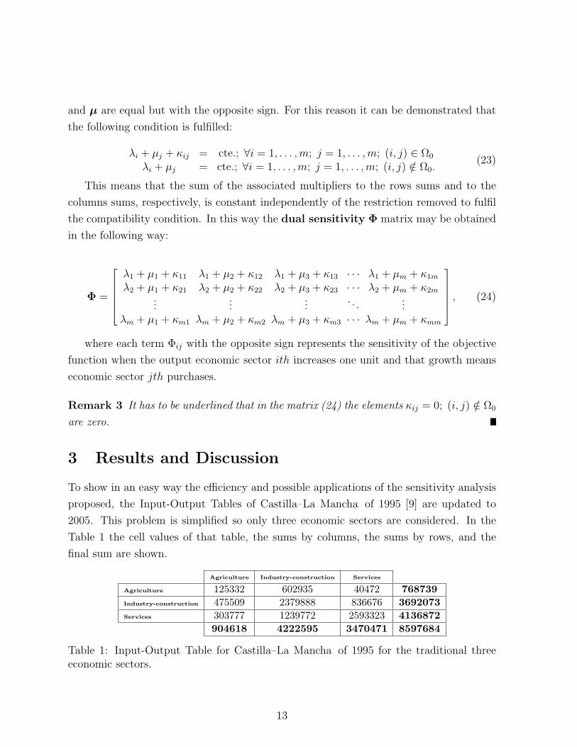
and µ are equal but with the opposite sign. For this reason it can be demonstrated that
the following condition is fulfilled:
λi + µj + κij = cte.; ∀i = 1, . . . ,m; j = 1, . . . ,m; (i, j) ∈ Ω0
λi + µj = cte.; ∀i = 1, . . . ,m; j = 1, . . . ,m; (i, j) /∈ Ω0.(23)
This means that the sum of the associated multipliers to the rows sums and to the
columns sums, respectively, is constant independently of the restriction removed to fulfil
the compatibility condition. In this way the dual sensitivity Φ matrix may be obtained
in the following way:
Φ =
λ1 + µ1 + κ11 λ1 + µ2 + κ12 λ1 + µ3 + κ13 · · · λ1 + µm + κ1m
λ2 + µ1 + κ21 λ2 + µ2 + κ22 λ2 + µ3 + κ23 · · · λ2 + µm + κ2m...
......
. . ....
λm + µ1 + κm1 λm + µ2 + κm2 λm + µ3 + κm3 · · · λm + µm + κmm
, (24)
where each term Φij with the opposite sign represents the sensitivity of the objective
function when the output economic sector ith increases one unit and that growth means
economic sector jth purchases.
Remark 3 It has to be underlined that in the matrix (24) the elements κij = 0; (i, j) /∈ Ω0
are zero.
3 Results and Discussion
To show in an easy way the efficiency and possible applications of the sensitivity analysis
proposed, the Input-Output Tables of Castilla–La Mancha of 1995 [9] are updated to
2005. This problem is simplified so only three economic sectors are considered. In the
Table 1 the cell values of that table, the sums by columns, the sums by rows, and the
final sum are shown.
Agriculture Industry-construction Services
Agriculture 125332 602935 40472 768739Industry-construction 475509 2379888 836676 3692073Services 303777 1239772 2593323 4136872
904618 4222595 3470471 8597684
Table 1: Input-Output Table for Castilla–La Mancha of 1995 for the traditional threeeconomic sectors.
13

If the primal and dual problems are solved the solution shown in Table 2 is obtained,
that is, the Input-Output Tables of Castilla–La Mancha for 2005, where the sums by
columns and the sums by rows also appear.
The following Table 3 shows the changes (%) in the transactions among the different
economic sectors, and changes in the sums by rows, the sums by columns and the total
sum, respectively.
It is relevant to note that the larger growths are associated to the interchanges between
the economic sectors “Industry-construction” and “Services”. It is also important to state
that the dual variable associated to the first column sum restraint is zero, as it is shown
in the particular solution in (18).
Agriculture Industry-construction Services λ
Agriculture 107445 887953 62348 −0.8460 1057746Industry-construction 565818 4864845 1789041 −1.1739 7219704Services 337650 2367270 5179801 −1.1057 7884720µ 0 −0.5411 −0.5861
1010913 8120067 7031190 16691930
Table 2: Primal y dual solutions of the RAS problem, and sums by rows and by columnsof the final matrix.
Agriculture Industry-construction Services
Agriculture -14.3 47.3 54.1 37.6Industry-construction 19.0 104.4 113.8 95.5Services 11.2 90.9 99.7 90.6
11.8 92.3 102.6 88.0
Table 3: Changes (%) in the transactions among the different economic sectors, andchanges in the sums by rows, the sums by columns and the total sum.
The Table 4 shows the sensitivities of the “distance” between the 1995 and 2005
Castilla–La Mancha matrixes with respect to the changes in the total output and pur-
chases in 2005 in Castilla–La Mancha. In this way, when there is an unitary increase
in the output of “Industry-construction” adquired by the rest of the economic sectors
(u1 = u1 +1), if this output is purchased by the “Services” economic sector (v3 = v3 +1),
the increase of the objective function is 1.76. This value shows us the relation between the
regional economic development and the different economic transactions inside a region; in
this way we could outline which is the best strategy to induce a larger regional economic
development.
14

∂f∂u + ∂f
∂v Agriculture Industry-construction Services
Agriculture 0.8460 1.3871 1.4321Industry-construction 1.1739 1.7150 1.7600Services 1.1057 1.6468 1.6918
Table 4: Objective function derivatives with respect to the changes in u and v.
In the same way Figure 2 shows the derivatives of optimum values of the Input-Output
Table for Castilla–La Mancha 2005 when the total output and purchases change at the
same time for 2005. It has to be underlined that the sensitivity values are bigger in the
diagonal in the sense that in a specific economic interchange zij the greatest increase in
its optimum value happens when the sales of economic sector i th to the rest ui = ui + 1
of economic sectors fit in with an increase in the purchases of economic sector j th to
the rest of the sectors vj = vj + 1. It is interesting to underline that, for example, in the
case of “Agriculture” and “Services” interchange (z13), the maximum increase is lower
than 0.08 euros for all the combinations between total sales and purchases in 2005, much
lower values than for the rest of the interchanges and a sign of the scarce growth of this
term with respect to the changes in those total sales and purchases. An important issue
in these sensitivities is that if we sum the values of all these graphs the result will be an
unitary matrix in the way that:
m∑i=1
m∑j=1
(∂zij
∂uk
+∂zij
∂vl
)= 1; ∀k = 1, . . . , n; l = 1, . . . , n. (25)
This expression means that an increase of one euro in the sales of k th economic
sector to the rest of the sectors uk = uk + 1, that involves an increase in the purchases
of l th economic sector to the rest of the sectors vl = vl + 1, provoke that the increase
of one euro is distributed among the intersectoral interchanges. For example, if there is
an increase of one euro in the sales of “Agriculture” to the rest of the economic sectors
(u1 = u1 + 1), and these sales correspond to purchases of the “Agriculture” economic
sector to the rest of the sectors (v1 = v1 + 1), the largest sale-purchase growth is between
“Industry-construction” and “Agriculture”, due to the bigger value of (1, 1) in the graph
Z21 with respect to the rest of the graphs. With this information we can know which is
the best economic strategy to obtain the largest possible growth in a specific transaction
value, and how this change affects the rest of the transactions.
As a last analysis we can mention the Table 5 where the sensitivities of the economic
transactions optimum values with respect to the weights are shown. As it can be seen the
absolute larger values are in the matrix diagonal, what involves that the increase in the
15

(1,1)(1,2) (2,1) (2,3) (3,2)
(1,3) (2,2) (3,1) (3,3)0.05
0
0.05
0.1
0.15
0.2
0.5
0
0.5
1
0.02
0
0.02
0.04
0.06
0.08
0.2
0
0.2
0.4
0.6
0.5
0
0.5
1
0.4
0.2
0
0.2
0.4
0.6
0.1
0
0.1
0.2
0.3
0.4
0.5
0
0.5
1
0.5
0
0.5
1
(1,1)(1,2) (2,1) (2,3) (3,2)
(1,3) (2,2) (3,1) (3,3) (1,1)(1,2) (2,1) (2,3) (3,2)
(1,3) (2,2) (3,1) (3,3)
(1,1)(1,2) (2,1) (2,3) (3,2)
(1,3) (2,2) (3,1) (3,3)
(1,1)(1,2) (2,1) (2,3) (3,2)
(1,3) (2,2) (3,1) (3,3)(1,1)(1,2) (2,1) (2,3) (3,2)
(1,3) (2,2) (3,1) (3,3)(1,1)(1,2) (2,1) (2,3) (3,2)
(1,3) (2,2) (3,1) (3,3)
(1,1)(1,2) (2,1) (2,3) (3,2)
(1,3) (2,2) (3,1) (3,3) (1,1)(1,2) (2,1) (2,3) (3,2)
(1,3) (2,2) (3,1) (3,3)
z11
ui
z11
vj+
z22
ui
z22
vj+
z23
ui
z23
vj+
z33
ui
z33
vj+z32
ui
z32
vj+
z21
ui
z21
vj+
z31
ui
z31
vj+
z12
ui
z12
vj+
z13
ui
z13
vj+
Figure 2: Sensitivity values of the optimum values of the cell elements of the Input-OutputTable of Castilla–La Mancha 2005 with respect to the changes in the sums by columnsand by rows.
16

weight of one specific economic transaction entails a bigger reduction in that transaction.
∂wij
∂wklw11 w12 w13 w21 w22 w23 w31 w32 w33
z11 −86305 80039 6266 54145 −53130 −1015 32160 −26910 −5250z12 80039−131365 51325 −51818 75629 −23812 −28222 55735 −27514z13 6266 51325−57591 −2327 −22500 24827 −3938 −28826 32764z21 54145 −51818 −2327−231205 141529 89676 177060 −89711 −87350z22 −53130 75630 −22500 141529 −828060 686532 −88400 752431 −664032z23 −1015 −23812 24827 89676 686532−776207.7 −88661 −662720 751381z31 32160 −28222 −3938 177060 −88399 −88661.0−209220 116621 92599z32 −26910 55735 −28826 −89711 752431 −662719.9 116621−808166 691545z33 −5250 −27514 32764 −87349−664031.9 751380.9 92600 691545−784145
Table 5: Derivatives of the optimum elements of the Input-Output Table of Castilla–LaMancha 2005 with respect to the weights.
The information supplied by Table 5 is really useful and, for example, it indicates
that an increase of one unity in the weight associated to the intrasectoral transactions
in “Industry-construction” (w22) involves a decrease in the intrasectoral transactions in
“Industry-construction” (z22) of −828060 euros and “Services” (z33) of −664031.9 euros,
respectively, and an increase in the intersectoral transactions (z23) of 686532 euros and
(z32) of 752431 euros.
4 Conclusions
This paper provides a procedure for solving the primal and dual weighted RAS method,
obtaining not only the optimal solution of the primal problem but information of the
sensitivities of the solution with respect the parameters. The main conclusions derived
from the work reported can be summarized as follows:
1. Due to the excess of constraints in the mathematical definition of the RAS problem
the dual problem has infinite solutions; for this, a new procedure to obtain a unique
solution of the dual problem holding the compatibility condition is provided.
2. It turns out that this unique solution of the dual problem allows obtaining the sen-
sitivity matrix, invariant sensitivities (measurements) of the primal RAS objective
function with respect constraint parameters.
3. The meaning of the sensitivity matrix obtained is very useful for the economic
analysis. That matrix shows us which is the influence of the interchanges between
economic sectors in the development of the economic structure of a certain region,
17
in the case of updating I-O tables, and the influence of those interchanges in the
regional economic singularity in a national context in the case of regionalizing I-O
tables.
4. The solution of the dual problem can be obtained efficiently once the solution of the
primal RAS problem is known using an iterative method.
5. In Castilla–La Mancha during the last ten years, the economic interchange which
has made a major contribution to the regional development has been the purchases
made by “services” to “industry-construction”.
References
[1] Bazaraa, M. S., Jarvis, J. J. and Sherali, H. D. (1990). Linear Programming
and Network Flows second ed. John Wiley & Sons, New York.
[2] Bazaraa, M. S., Sherali, H. D. and Shetty, C. M. (1993). Nonlinear Pro-
gramming. Theory and Algorithms second ed. John Wiley & Sons, New York.
[3] Bjerager, P. and Krenk, S. (1989). Parametric sensitivity in first order relia-
bility theory. J. Engineering Mechanics, ASCE 115, 1577–1582.
[4] Castillo, E., Cobo, A., Jubete, F. and Pruneda, R. E. (1999). Orthogonal
Sets and Polar Methods in Linear Algebra: Applications to Matrix Calculations,
Systems of Equations and Inequalities, and Linear Programming. John Wiley &
Sons, New York.
[5] Castillo, E., Cobo, A., Jubete, F., Pruneda, R. E. and C., C. (2000).
An orthogonally based pivoting transformation of matrices and some applications.
SIAM Journal on Matrix Analysis and Applications 22, 666–681.
[6] Castillo, E., Conejo, A., Pedregal, P., Garcıa, R. and Alguacil, N.
(2001). Building and Solving Mathematical Programming Models in Engineering and
Science. John Wiley & Sons Inc., New York. Pure and Applied Mathematics: A
Wiley-Interscience Series of Texts, Monographs and Tracts.
[7] Castillo, E. and Jubete, F. (2004). The γ-algorithm and some applications.
International Journal of Mathematical Education in Science and Technology 369–
389.
18

[8] Castillo, E., Jubete, F., Pruneda, E. and Solares, C. (2002). Obtaining
simultaneous solutions of linear subsystems of equations and inequalities. Linear
Algebra and its Applications 131–154.
[9] CESCLM (2003). Tablas input-output de Castilla-La Mancha. Consejo Econmico y
Social de Castilla-La Mancha, Toledo.
[10] Conejo, A., Castillo, E., Mınguez, R. and Garcıa-Bertrand, R. (2006).
Decomposition techniques in mathematical programming. Engineering and science
applications. Springer Berlin Heidelberg, New York.
[11] Enevoldsen, I. (1994). Sensitivity analysis of reliability-based optimal solution.
Journal of Engineering Mechanics 120, 198–205.
[12] Luenberger, D. G. (1989). Linear and Nonlinear Programming second ed.
Addison-Wesley, Reading, Massachusetts.
[13] Miller, R. E. (1998). Methods of Interregional and Regional Analysis. Ashgate,
Brookfield, VE, USA. ch. Regional and interregional input-output analysis, pp. 41–
133.
[14] Miller, R. E. and Blair, P. D., Eds. (1985). Input-output analysis : Foundations
and extensions. Prentice-Hall, Englewood Cliffs, NJ, USA.
[15] Padberg, M. (1995). Linear Optimization and Extensions. Springer, Berlin, Ger-
many.
[16] Press, W. H., Teukolsky, S. A., Vetterling, W. T. and Flannery, B. P.
(1992). Numerical Recipes in C. Cambridge University Press, New York.
[17] Roos, C., Terlaky, T. and Vial, J. P. (1997). Theory and Algorithms for
Linear Optimization: An Interior Point Approach. John Wiley & Sons, Chichester,
UK. Wiley-Interscience Series in Discrete Mathematics and Optimization.
[18] Sobieski, J. S., Barthelemy, J. F. and Riley, K. M. (1982). Sensitivity of
optimal solutions of problems parameters. AIAA J. 20, 1291–1299.
[19] Sorensen, J. D. and Enevoldsen, I. (1992). Sensitivity analysis in reliability-
based shape optimization. In NATO ASI. ed. B. H. V. Topping. vol. 2 21 of E.
Kluwer Academic Publishers, Dordrecht, The Nethelands. pp. 617–638.
19

[20] Vanderplaats, G. N. (1984). Numerical Optimization Techniques for Engineering
Design. McGraw-Hill, New York.
20