Analysis of stochastic local search methods for the

unrelated parallel machine scheduling problem

Haroldo G. Santos∗a, Tulio A.M. Toffoloa,b,Cristiano L.T. Silvaa, and Greet Vanden Bergheb

aFederal University of Ouro Preto, Department of Computing - BrazilbKU Leuven, Department of Computer Science, CODeS & iMinds-ITEC - Belgium

Abstract

This work addresses the unrelated parallel machine scheduling problem withsequence-dependent setup times, in which a set of jobs must be scheduled for ex-ecution by one of several available machines. Each job has a machine-dependentprocessing time. Furthermore, given multiple jobs, there are additional setuptimes, which vary based on the sequence and machine employed. The objec-tive is to minimize the schedule’s completion time (makespan). The problemis NP-hard and of significant practical relevance. The present paper investi-gates the performance of four different stochastic local search (SLS) methodsdesigned towards solving the particular scheduling problem: Simulated Anneal-ing, Iterated Local Search, Late Acceptance Hill-Climbing and Step CountingHill-Climbing. The analysis focuses on design questions, tuning effort and op-timization performance. Simple neighborhood structures are considered. Allproposed SLS methods performed significantly better than two state-of-the-arthybrid heuristics, especially for larger instances. Updated best-known solutionswere generated for 901 out of the 1,000 large benchmark instances considered,demonstrating that particular stochastic local search methods are simple yetpowerful alternatives to current approaches for addressing the problem. Im-plementations of the contributed algorithms have been made available to theresearch community.

1 Introduction

The present paper investigates different stochastic local search (SLS) methods for theunrelated parallel machine scheduling problem with sequence-dependent setup times(UPMSP). In this problem, a set of jobs must be executed by a set of machines. Eachjob has a processing time associated with each machine and the setup time betweentwo jobs is both sequence and machine-dependent. The objective is to minimize thecompletion time of all jobs, called makespan.

The UPMSP is a generalization of many classical parallel machine scheduling prob-lems. It is highly relevant in production planning, when considering production lineswith heterogeneous machines. The problem is extremely computationally challenging

∗Corresponding author. E-mail: haroldo@iceb.ufop.br

1

and most instances in the literature are unsolved. Indeed, no proven optimal solutionsare known for the 1,000 largest instances in the benchmark set proposed by Valladaand Ruiz (2011).

Recent literature indicates that hybrid methods are generally employed to ap-proach the UPMSP. These methods incorporate ideas from several metaheuristics inthe quest of producing better solvers. Such hybridized approaches have numerousdisadvantages: : (i) they generally require many parameters to tune; (ii) by execut-ing several optimization phases, these methods tend to be computationally expensive;(iii) it is difficult to identify which parts of the solver are the most effective and, mostimportantly, (iv) there is a well known statistical correlation (McConnell, 2004) insoftware industry where the number of bugs grows proportionally with respect to thenumber of lines of code: simple methods are more likely to be implemented withoutbugs than more complex ones, a very important consideration for operations researchpractitioners. The present paper investigates methods which contrast with this trend,by relying solely on simple local search. It is subsequently demonstrated how appro-priately implemented and tuned SLS methods produce high quality solutions in ashort length of time, outperforming other state of the art heuristic methods.

The investigation includes: (i) an analysis of parameter tuning challenges, (ii)a discussion and experiments on diversification and intensification strategies for theUPMSP, and (iii) improved best-known results.

The present paper is organized as follows. Section 2 presents the UPMSP in de-tail, including a literature review of heuristic methods. The neighborhoods used in allSLS methods implemented are described in Section 3. Section 4 details the construc-tive algorithm and the design of the four stochastic local search methods we tested:Simulated Annealing, Late Acceptance Hill-Climbing, Step Counting Hill-Climbingand Iterated Local Search. Section 5 presents an extensive computational study ofparameter tuning for these methods and the obtained results. Finally, conclusionsare discussed in Section 6.

2 Problem description and literature review

The UPMSP is denoted as R|Sijk|Cmax in the α|β|γ notation introduced by Gra-ham et al. (1979). It is a generalization of the parallel machine scheduling problemP ||Cmax, and therefore computationally challenging (NP-hard) even when only twomachines are considered (Garey and Johnson, 1979). A complete survey on schedulingproblems with setup times, including a discussion on the main algorithmic approaches,is presented by Allahverdi et al. (2008). The following notation is used to refer to theUPMSP:

Let J = {j1, ..., jn} be the set of n jobs and M = {m1, ...,mk} the set of kmachines, such that:

1. each job j must be executed exactly once and by only one machine;

2. each job j has a processing time pmj if executed by machine m;

3. machine m requires smij setup time to execute job j directly after job i;

4. machine m requires smii setup time to execute job i if i is its initial job.

2

The problem’s objective is to allocate all jobs in J to the machines in M such thatthe completion time of the last job (makespan) is as early as possible. The machineexecuting the last job is hereafter called the makespan machine.

Kim et al. (2002) presented an interesting application of the UPMSP in the com-pound semiconductor wafer industry. The dicing operation of semiconductor wafersinvolves the processing of wafers on several machines with different technologies andmanufacturers. Each machine must be prepared according to the type of wafer tobe processed. There is a resulting setup time that is both machine and sequence-dependent.

Rabadi et al. (2006) implemented a Greedy Randomized Adaptive Search Pro-cedure (GRASP) (Feo and Resende, 1995) style algorithm and also generated someinstances. De Paula et al. (2007) and Avalos-Rosales et al. (2015) also proposedGRASP-like algorithms combined with Variable Neighborhood Search (Hansen andMladenovic, 1997).

Vallada and Ruiz (2011) proposed a set of challenging instances for the problem(SOA-2011). They designed a genetic algorithm (Goldberg, 1989) combined with lo-cal search, which they describe as capable of achieving good results within a smallamount of time. Their results significantly improved upon those obtained by Rabadiet al. (2006). More recently, Cota et al. (2014) proposed a multi-neighborhood hybridmetaheuristic including path relinking (Glover et al., 2000) for polishing solutions.Their results generally improved the original results of Vallada and Ruiz (2011), pre-senting new best solutions for most instances.

The application of exact integer programming solvers was evaluated in Avalos-Rosales et al. (2013), using integer programming reformulations. Improvements wereobtained when solving the set of small instances with less than 50 jobs proposed byVallada and Ruiz (2011).

3 Neighborhood structures

The fundamental parts of any local search method are the neighborhood structures.Before detailing any specifics, certain characteristics of the UPMSP should be men-tioned:

• only changes involving the makespan machine can improve a solution;

• to escape from local optima, a sequence of modifications involving differentmachines may be needed, such as: swapping jobs between machines or alteringthe processing sequence on these machines;

• depending on the instance characteristics, some neighborhoods may be moreimportant than others as the setup times of particular instances may be moresignificant than the processing times, and vice-versa.

Considering these characteristics, strategies to intensify and diversify the searchwere developed. The first aspect that defines each strategy is the selection of the mainmachine involved in the neighbor generation, denoted hereafter as mx. Two possi-bilities are considered: (i) selecting a random machine as mx and (ii) selecting themakespan machine as mx. The second aspect that defines a neighborhood generation

3

strategy is the cardinality of the evaluated neighbor set. Again, two possibilities areconsidered:

1. regular policy: a single random neighbor solution is evaluated;

2. intensification policy: a small subset of neighbors is analyzed and the bestone is returned.

All possible combinations of these aspects – selection of machine mx and car-dinality of the evaluated neighbor set – generate four different neighbor generationstrategies. They all have the same probability of being chosen by the neighborhoodsat each iteration.

Six neighborhood structures were developed to explore the search space. To sim-plify the final algorithm, all neighborhoods have the same probability of being selectedduring the local search methods. These neighborhoods are covered in detail in thefollowing paragraphs.

Shift neighborhood

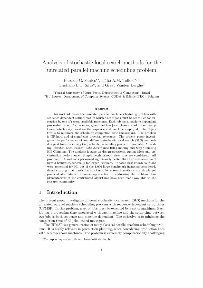
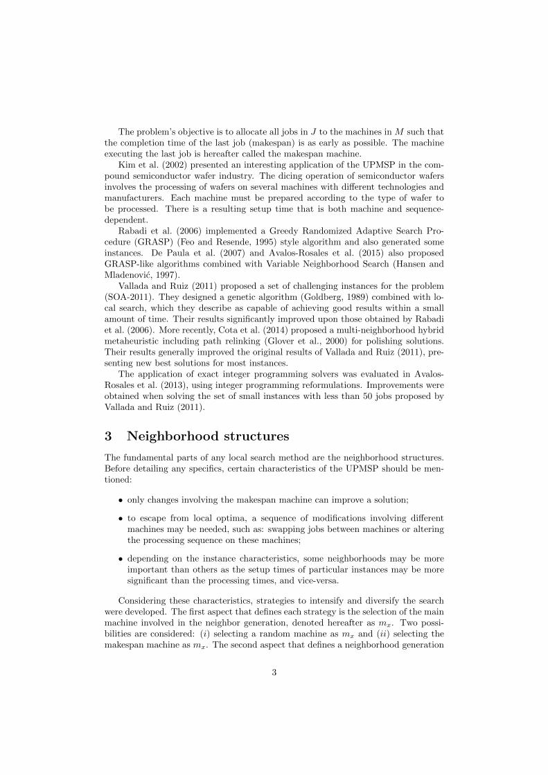
A neighbor in the shift neighborhood is generated by re-scheduling a random job froma machine mx to another position on the same machine. The position is randomlychosen, except when the intensification policy is selected. In this case, the targetposition of the job is greedily selected, whereby the position incurring the shortestmakespan for the machine is chosen. Figure 1 shows how a shift neighbor is generated.

j2j1 j2 j3 j4 j5 j1j3 j4 j5mx mx

Figure 1: Example of a neighbor in the shift neighborhood.

Switch neighborhood

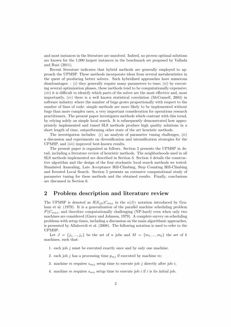
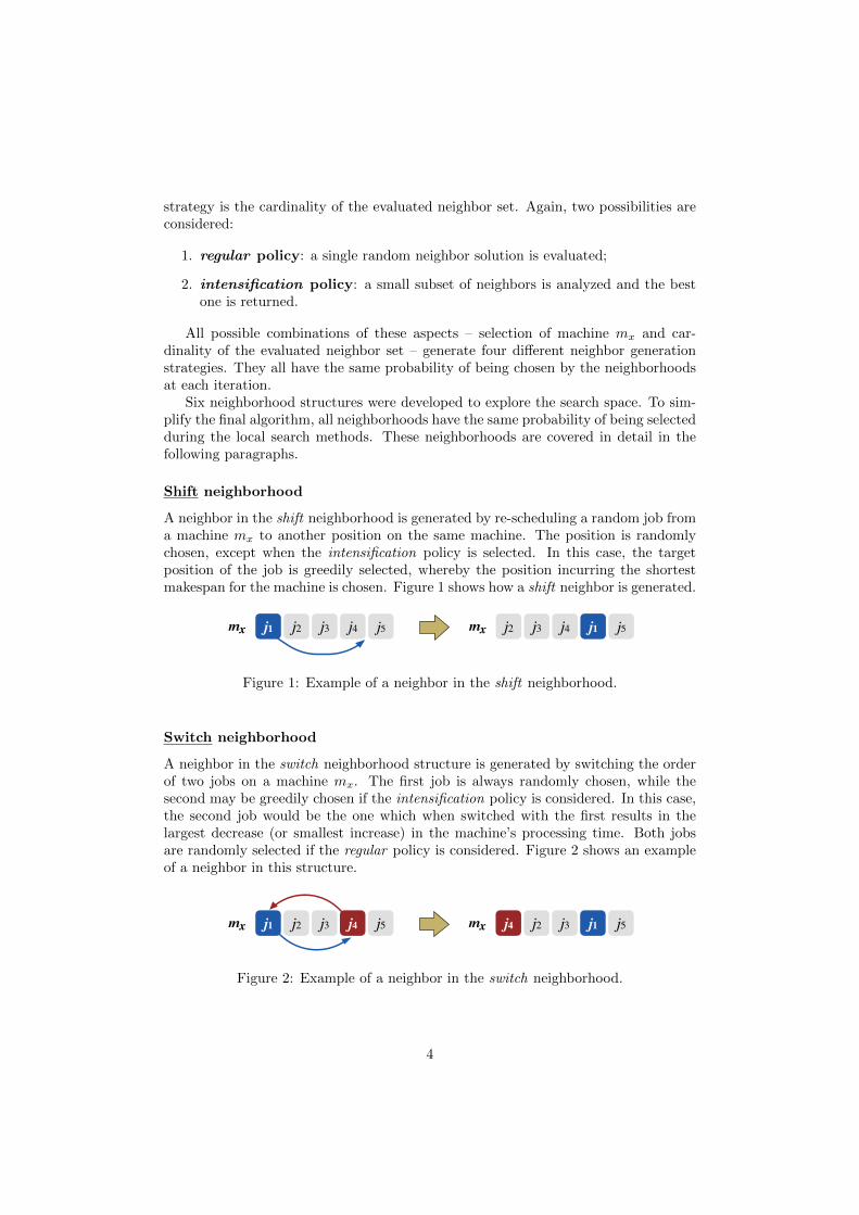
A neighbor in the switch neighborhood structure is generated by switching the orderof two jobs on a machine mx. The first job is always randomly chosen, while thesecond may be greedily chosen if the intensification policy is considered. In this case,the second job would be the one which when switched with the first results in thelargest decrease (or smallest increase) in the machine’s processing time. Both jobsare randomly selected if the regular policy is considered. Figure 2 shows an exampleof a neighbor in this structure.

j1 j2 j3 j4 j5 j4 j2 j3 j1 j5mx mx

Figure 2: Example of a neighbor in the switch neighborhood.

4

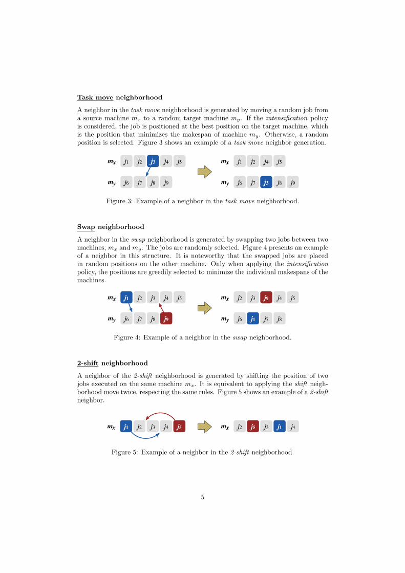
Task move neighborhood

A neighbor in the task move neighborhood is generated by moving a random job froma source machine mx to a random target machine my. If the intensification policyis considered, the job is positioned at the best position on the target machine, whichis the position that minimizes the makespan of machine my. Otherwise, a randomposition is selected. Figure 3 shows an example of a task move neighbor generation.

j1 j2 j3 j4 j5

j6 j7 j8 j9 j7

j1 j2 j4 j5

j6 j8 j9j3

mx

my

mx

my

Figure 3: Example of a neighbor in the task move neighborhood.

Swap neighborhood

A neighbor in the swap neighborhood is generated by swapping two jobs between twomachines, mx and my. The jobs are randomly selected. Figure 4 presents an exampleof a neighbor in this structure. It is noteworthy that the swapped jobs are placedin random positions on the other machine. Only when applying the intensificationpolicy, the positions are greedily selected to minimize the individual makespans of themachines.

j1 j2 j3 j4 j5

j6 j7 j8 j9 j1

j2 j3 j4 j5

j6 j7 j8

j9mx

my

mx

my

Figure 4: Example of a neighbor in the swap neighborhood.

2-shift neighborhood

A neighbor of the 2-shift neighborhood is generated by shifting the position of twojobs executed on the same machine mx. It is equivalent to applying the shift neigh-borhood move twice, respecting the same rules. Figure 5 shows an example of a 2-shiftneighbor.

j2j1 j2 j3 j4 j5 j5 j3 j1 j4mx mx

Figure 5: Example of a neighbor in the 2-shift neighborhood.

5

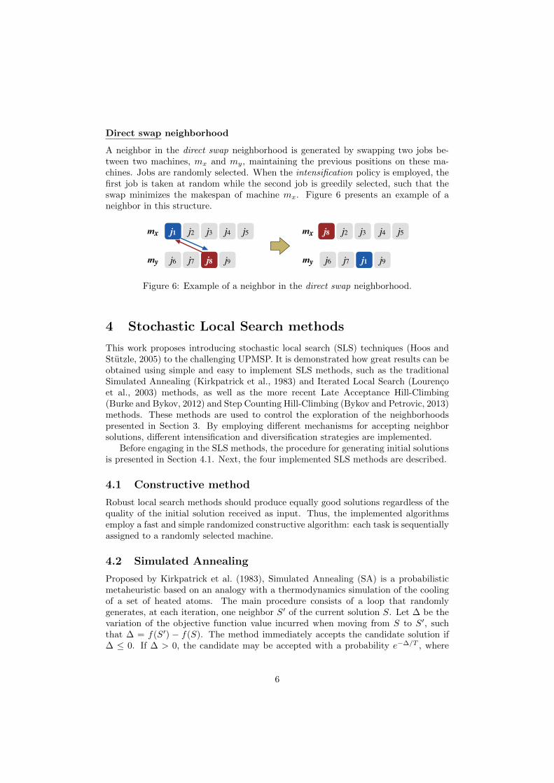
Direct swap neighborhood

A neighbor in the direct swap neighborhood is generated by swapping two jobs be-tween two machines, mx and my, maintaining the previous positions on these ma-chines. Jobs are randomly selected. When the intensification policy is employed, thefirst job is taken at random while the second job is greedily selected, such that theswap minimizes the makespan of machine mx. Figure 6 presents an example of aneighbor in this structure.

j1 j2 j3 j4 j5

j6 j7 j8 j9 j1

j2 j3 j4 j5

j6 j7 j9

j8mx

my

mx

my

Figure 6: Example of a neighbor in the direct swap neighborhood.

4 Stochastic Local Search methods

This work proposes introducing stochastic local search (SLS) techniques (Hoos andStutzle, 2005) to the challenging UPMSP. It is demonstrated how great results can beobtained using simple and easy to implement SLS methods, such as the traditionalSimulated Annealing (Kirkpatrick et al., 1983) and Iterated Local Search (Lourencoet al., 2003) methods, as well as the more recent Late Acceptance Hill-Climbing(Burke and Bykov, 2012) and Step Counting Hill-Climbing (Bykov and Petrovic, 2013)methods. These methods are used to control the exploration of the neighborhoodspresented in Section 3. By employing different mechanisms for accepting neighborsolutions, different intensification and diversification strategies are implemented.

Before engaging in the SLS methods, the procedure for generating initial solutionsis presented in Section 4.1. Next, the four implemented SLS methods are described.

4.1 Constructive method

Robust local search methods should produce equally good solutions regardless of thequality of the initial solution received as input. Thus, the implemented algorithmsemploy a fast and simple randomized constructive algorithm: each task is sequentiallyassigned to a randomly selected machine.

4.2 Simulated Annealing

Proposed by Kirkpatrick et al. (1983), Simulated Annealing (SA) is a probabilisticmetaheuristic based on an analogy with a thermodynamics simulation of the coolingof a set of heated atoms. The main procedure consists of a loop that randomlygenerates, at each iteration, one neighbor S′ of the current solution S. Let ∆ be thevariation of the objective function value incurred when moving from S to S′, suchthat ∆ = f(S′) − f(S). The method immediately accepts the candidate solution if∆ ≤ 0. If ∆ > 0, the candidate may be accepted with a probability e−∆/T , where

6

T is a parameter called temperature, which regulates the probability of acceptingworsening solutions.

The temperature is initially set to a value t0. After a fixed number of iterationssamax, the temperature is gradually lowered by a cooling rate α. The temperature ina stage q is given by tq ← α × tq−1, with 0 < α < 1 (geometric cooling). With thisprocedure, a greater chance of avoiding local optima occurs at the initial iterationand as t approaches zero the algorithm behaves like a descent method, reducingthe likelihood of accepting worsening solutions (Henderson et al., 2003). To preventstagnation, reheating may be performed when the temperature reaches a minimumthreshold ε.

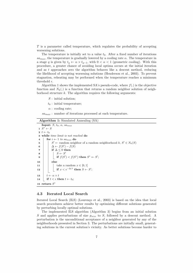
Algorithm 1 shows the implemented SA’s pseudo-code, where f(.) is the objectivefunction and Nk(.) is a function that returns a random neighbor solution of neigh-borhood structure k. The algorithm requires the following arguments:

S : initial solution;

t0 : initial temperature;

α : cooling rate;

samax : number of iterations processed at each temperature.

Algorithm 1: Simulated Annealing (SA)

Input: S, t0, α, samax

1 S∗ ← S2 t← t03 while time limit is not reached do4 for i← 1 to samax do5 S′ ← random neighbor of a random neighborhood k, S′ ∈ Nk(S)6 ∆← f(S′)− f(S)7 if ∆ ≤ 0 then8 S ← S′

9 if f(S′) < f(S∗) then S∗ ← S′;

10 else11 take a random x ∈ [0, 1]

12 if x < e−∆/t then S ← S′;

13 t← α× t14 if t < ε then t← t0;

15 return S∗

4.3 Iterated Local Search

Iterated Local Search (ILS) (Lourenco et al., 2003) is based on the idea that localsearch procedures achieve better results by optimizing different solutions generatedby perturbing locally optimal solutions.

The implemented ILS algorithm (Algorithm 3) begins from an initial solutionS and applies perturbations of size psize to S, followed by a descent method. Aperturbation is the unconditional acceptance of a neighbor generated by any of theneighborhoods presented in Section 3. The perturbations are initially small, generat-ing solutions in the current solution’s vicinity. As better solutions become harder to

7

find, the perturbation increases so that solutions farther than the current one can bereached, resulting in diversification.

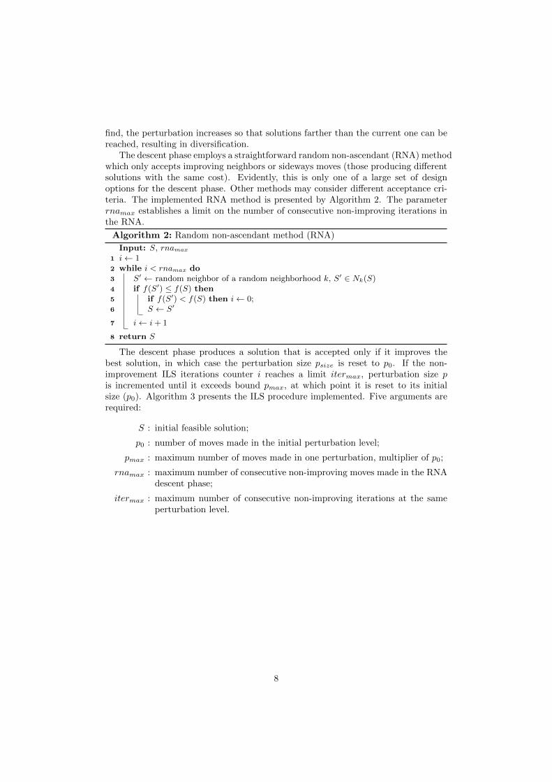
The descent phase employs a straightforward random non-ascendant (RNA) methodwhich only accepts improving neighbors or sideways moves (those producing differentsolutions with the same cost). Evidently, this is only one of a large set of designoptions for the descent phase. Other methods may consider different acceptance cri-teria. The implemented RNA method is presented by Algorithm 2. The parameterrnamax establishes a limit on the number of consecutive non-improving iterations inthe RNA.

Algorithm 2: Random non-ascendant method (RNA)

Input: S, rnamax

1 i← 12 while i < rnamax do3 S′ ← random neighbor of a random neighborhood k, S′ ∈ Nk(S)4 if f(S′) ≤ f(S) then5 if f(S′) < f(S) then i← 0;6 S ← S′

7 i← i+ 1

8 return S

The descent phase produces a solution that is accepted only if it improves thebest solution, in which case the perturbation size psize is reset to p0. If the non-improvement ILS iterations counter i reaches a limit itermax, perturbation size pis incremented until it exceeds bound pmax, at which point it is reset to its initialsize (p0). Algorithm 3 presents the ILS procedure implemented. Five arguments arerequired:

S : initial feasible solution;

p0 : number of moves made in the initial perturbation level;

pmax : maximum number of moves made in one perturbation, multiplier of p0;

rnamax : maximum number of consecutive non-improving moves made in the RNAdescent phase;

itermax : maximum number of consecutive non-improving iterations at the sameperturbation level.

8

Algorithm 3: Iterated Local Search (ILS)

Input: S, p0, pmax, rnamax, itermax

1 S∗ ← S ← RNA(S, rnamax)2 i← 03 p← p0

4 pmax ← p0 × pmax

5 while time limit is not reached do6 for j ← 1 to p do7 S ← random neighbor S′ of a random neighborhood k, S′ ∈ Nk(S)

8 S ← RNA(S, rnamax)9 if f(S) < f(S∗) then

10 S∗ ← S11 i← 012 p← p0

13 else14 S ← S∗

15 i← i+ 1

16 if i ≥ itermax then17 i← 018 p← p+ p0

19 if p > pmax then p← p0;

20 return S∗

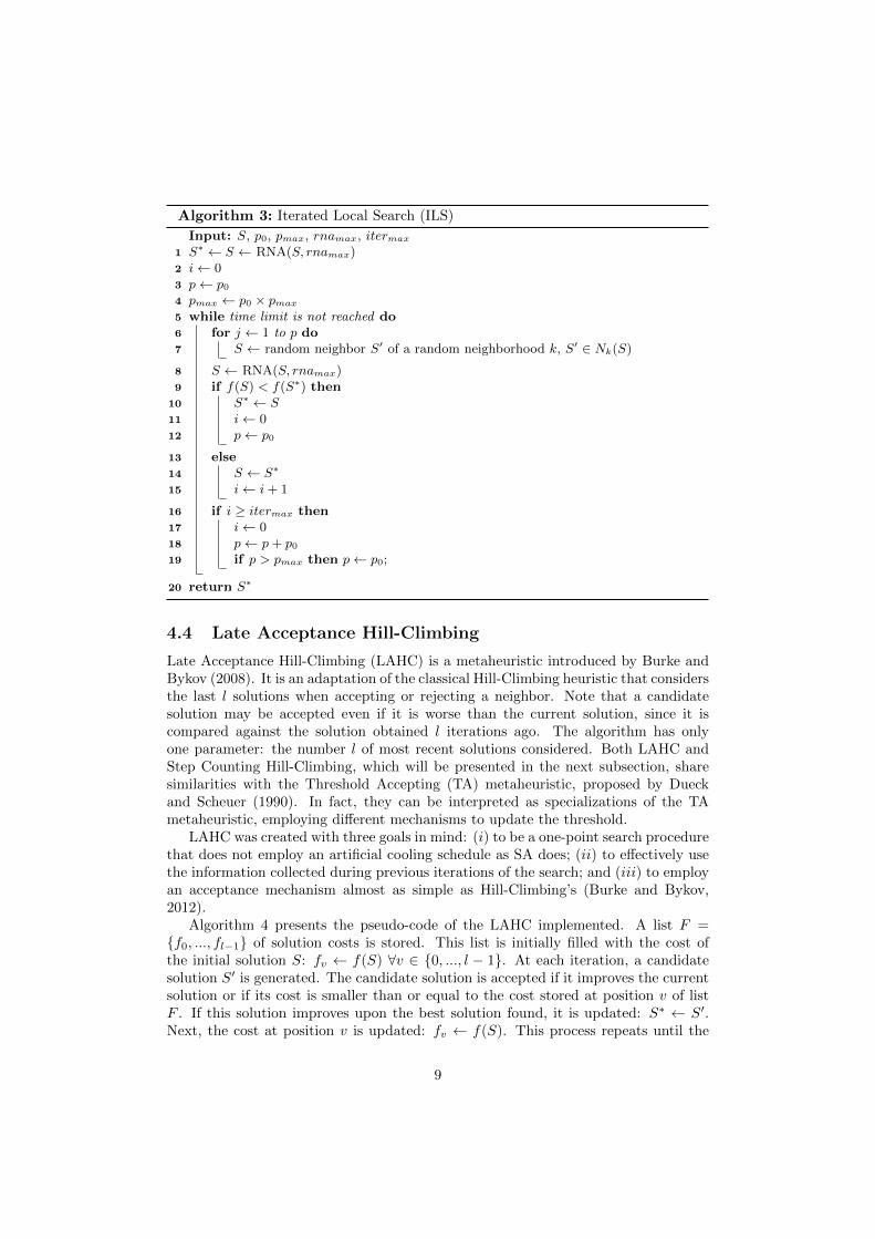
4.4 Late Acceptance Hill-Climbing

Late Acceptance Hill-Climbing (LAHC) is a metaheuristic introduced by Burke andBykov (2008). It is an adaptation of the classical Hill-Climbing heuristic that considersthe last l solutions when accepting or rejecting a neighbor. Note that a candidatesolution may be accepted even if it is worse than the current solution, since it iscompared against the solution obtained l iterations ago. The algorithm has onlyone parameter: the number l of most recent solutions considered. Both LAHC andStep Counting Hill-Climbing, which will be presented in the next subsection, sharesimilarities with the Threshold Accepting (TA) metaheuristic, proposed by Dueckand Scheuer (1990). In fact, they can be interpreted as specializations of the TAmetaheuristic, employing different mechanisms to update the threshold.

LAHC was created with three goals in mind: (i) to be a one-point search procedurethat does not employ an artificial cooling schedule as SA does; (ii) to effectively usethe information collected during previous iterations of the search; and (iii) to employan acceptance mechanism almost as simple as Hill-Climbing’s (Burke and Bykov,2012).

Algorithm 4 presents the pseudo-code of the LAHC implemented. A list F ={f0, ..., fl−1} of solution costs is stored. This list is initially filled with the cost ofthe initial solution S: fv ← f(S) ∀v ∈ {0, ..., l − 1}. At each iteration, a candidatesolution S′ is generated. The candidate solution is accepted if it improves the currentsolution or if its cost is smaller than or equal to the cost stored at position v of listF . If this solution improves upon the best solution found, it is updated: S∗ ← S′.Next, the cost at position v is updated: fv ← f(S). This process repeats until the

9

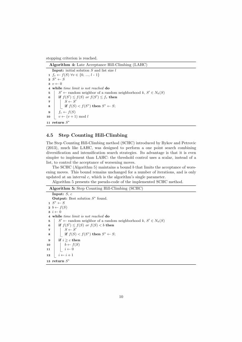
stopping criterion is reached.

Algorithm 4: Late Acceptance Hill-Climbing (LAHC)

Input: initial solution S and list size l1 fv ← f(S) ∀v ∈ {0, ..., l - 1}2 S∗ ← S3 v ← 04 while time limit is not reached do5 S′ ← random neighbor of a random neighborhood k, S′ ∈ Nk(S)6 if f(S′) ≤ f(S) or f(S′) ≤ fv then7 S ← S′

8 if f(S) < f(S∗) then S∗ ← S;

9 fv ← f(S)10 v ← (v + 1) mod l

11 return S∗

4.5 Step Counting Hill-Climbing

The Step Counting Hill-Climbing method (SCHC) introduced by Bykov and Petrovic(2013), much like LAHC, was designed to perform a one point search combiningdiversification and intensification search strategies. Its advantage is that it is evensimpler to implement than LAHC: the threshold control uses a scalar, instead of alist, to control the acceptance of worsening moves.

The SCHC (Algorithm 5) maintains a bound b that limits the acceptance of wors-ening moves. This bound remains unchanged for a number of iterations, and is onlyupdated at an interval c, which is the algorithm’s single parameter.

Algorithm 5 presents the pseudo-code of the implemented SCHC method.

Algorithm 5: Step Counting Hill-Climbing (SCHC)

Input: S, cOutput: Best solution S∗ found.

1 S∗ ← S2 b← f(S)3 i← 04 while time limit is not reached do5 S′ ← random neighbor of a random neighborhood k, S′ ∈ Nk(S)6 if f(S′) ≤ f(S) or f(S) < b then7 S ← S′

8 if f(S) < f(S∗) then S∗ ← S;

9 if i ≥ c then10 b← f(S)11 i← 0

12 i← i+ 1

13 return S∗

10

5 Computational experiments

This section presents an extensive experimental evaluation of the proposed SLS meth-ods. Experiments were conducted on the set of 1,640 benchmark instances proposedby Vallada and Ruiz (2011), for which best known solutions are recorded in SOA-ITI (2013). These instances have n ∈ {6, 8, 10, 12, 50, 100, 150, 200, 250} jobs andk ∈ {2, 3, 4, 5, 10, 15, 20, 25, 30} machines. Vallada and Ruiz (2011) divide these in-stances into two groups: small (n ≤ 12 and k ≤ 5) and large (n ≥ 50 and k ≥ 10).Processing times are uniformly distributed between {1, . . . , 99}. Considering the setuptimes, there are four groups of instances, with setup costs uniformly distributed inthe following ranges: {1, . . . , 9}, {1, . . . , 49}, {1, . . . , 99} and {1, . . . , 124}.

The algorithms were coded in Java 1.8 and the experiments were executed on anIntel R© CoreTMi7-4790 3.6Ghz computer with 16Gb of RAM memory, running theopenSUSE 13.2 linux operating system. This computer is approximately 2.5 timesfaster (PassMark software, 2015) at running sequential applications than the computerequipped with an Intel R© Core 2TMduo E6600 @ 2.4Ghz used by Vallada and Ruiz(2011) in their experiments.

Time limits in Vallada and Ruiz (2011) were computed as n × (k2 ) × t ms, with

t = 10, 30 and 50. To achieve a fair comparison between all algorithms, the time limitsof Vallada were scaled down by the factor suggested in the benchmarks of PassMarksoftware (2015). Consequently, all algorithms were executed with an approximatelyequal amount of processing power. When t = 50, for example, a time limit of 75seconds is imposed, whereas the execution time of Vallada and Ruiz (2011) was 187.5seconds. The authors wish to adhere to the guidelines of good laboratory practice foroptimization research (Kendall et al., 2016) and thus the source code and all solutionsare provided at http://www.goal.ufop.br/software/upmsp.

The evaluation of solutions employs a metric insensitive to scales: the relative per-centage deviation (RPD), presented in Equation 1. Vallada and Ruiz (2011) employedthe same metric1.

RPD = 100× Method solution− Best known solution

Best known solution(1)

The remainder of this section is organized as follows. A detailed parameter tuninginvestigation is discussed in Section 5.1. Section 5.2 analyses the impact of the variousneighborhoods. Finally, Section 5.3 presents the final results obtained by the SLSmethods and compares them with the state of the art methods in the literature.

5.1 Parameter tuning

A large set of experiments was conducted to discover the best parameter configurationfor each algorithm. The parameter tuning phase considered a separate training setof 164 randomly selected instances2, to avoid overfitting. All experiments, including

1Best known solutions were updated with the results obtained with the algorithms proposed bythe present paper.

2The instances in the training set were selected using the default random numbers generator inthe bash shell script programming language, version 4.2.

11

those considered during the parameter tuning phase, respected the same time limitspreviously detailed.

Firstly, a manually-selected set of values for each parameter was evaluated consid-ering its many combination with others. The objective is understanding the possiblecorrelations between parameters, while simultaneously evaluating each algorithm’ssensitivity to various parameter settings.

Secondly, the iRace package was used. This package implements the iterated rac-ing procedure (Lopez-Ibanez et al., 2011; Lopez-Ibanez and Stutzle, 2014), which isan extension of iterated F-race (I/F-Race) proposed by Birattari et al. (2007). Theprimary function of iRace is the automatic configuration of optimization algorithmsor, in other words, determining the most appropriate parameter settings for an opti-mization method. iRace is implemented as an R package (R Development Core Team,2008) and builds upon the race package.

5.1.1 Manual tuning

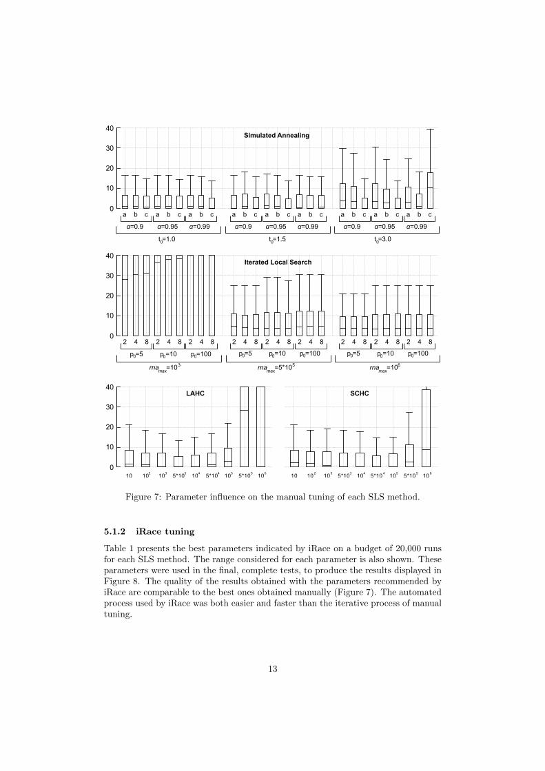
Figure 7 depicts the RPD obtained using different parameters settings for each of thefour implemented SLS methods.

Both LAHC and SCHC have only one parameter to tune. These methods weretested with l, c ∈ {10, 100, 1000, 5000, 10000, 50000, 100000, 500000, 1000000}. As pre-sented in Figure 7, SCHC appears less sensitive to parameter changes than LAHC.SCHC proves superior to LAHC given that it is not only easier to implement, butalso requires no additional memory structure.

Both SA and ILS have multiple parameters. During testing, various combinationsof parameter values were evaluated. SA was evaluated with 27 triples of the follow-ing parameters t0 ∈ {1, 1.5, 3}, α ∈ {0.9, 0.95, 0.99}, samax ∈ {1000, 10000, 100000}.In ILS 27 triples with rnamax ∈ {1000, 500000, 1000000}, p0 ∈ {5, 10, 100}, pmax ∈{2, 4, 8} (itermax was fixed in 1000) were tested. Figure 7 illustrates how this initialsampling of different parameters produced many low average RPDs for SA. Afterevaluating many iterations with different parameter combinations for the SA algo-rithm, it is observed that most combinations of different parameter values performedequally well. The implemented ILS was more sensitive to parameter changes: someparameter values significantly degenerated the quality of the produced RPDs. Theseconclusions, however, may be biased by the initial parameter sampling and by ourdifferent expertise in tuning these algorithms. To explore the search in the parame-ter space more systematically, all algorithms were submitted to an automated tuningprocedure, thus enabling an evaluation of how well a state of the art tuning algo-rithm discovers good parameter settings. These results are discussed in the followingsection.

12

0

10

20

30

40

10 10 10 5*10 10 5*10 10 5*10 10 10 10 10 5*10 10 5*10 10 5*10 10

0

10

20

30

40

a b c a b c a b c a b c a b c a b c a b c a b c a b c

0

10

20

30

40

1 2 3 4 5 6 7 8 9 10 11 12 13 14 15 16 17 18 19 20 21 22 23 24 25 26 27a b c a b c a b c a b c a b c a b c a b c a b c a b c

Simulated Annealing

LAHC SCHC

Iterated Local Search

0

10

20

30

40

10 10 10 5*10 10 5*10 10 5*10 10 10 10 10 5*10 10 5*10 10 5*10 102 3 3 4 4 55 6 2 3 3 4 4 55 6

α=0.9 α=0.95 α=0.99 α=0.9 α=0.95 α=0.99 α=0.9 α=0.95 α=0.99

p =5 p =10 p =100

2 4 8 2 4 8 2 4 8 2 4 8 2 4 8 2 4 8 2 4 8 2 4 8 2 4 8

0 0 0 p =5 p =10 p =1000 0 0 p =5 p =10 p =1000 0 0

t =1.5 0t =1.0 0 t =3.0 0

rna =5*10 max

5 rna =10 max

6rna =10max

3

Figure 7: Parameter influence on the manual tuning of each SLS method.

5.1.2 iRace tuning

Table 1 presents the best parameters indicated by iRace on a budget of 20,000 runsfor each SLS method. The range considered for each parameter is also shown. Theseparameters were used in the final, complete tests, to produce the results displayed inFigure 8. The quality of the results obtained with the parameters recommended byiRace are comparable to the best ones obtained manually (Figure 7). The automatedprocess used by iRace was both easier and faster than the iterative process of manualtuning.

13

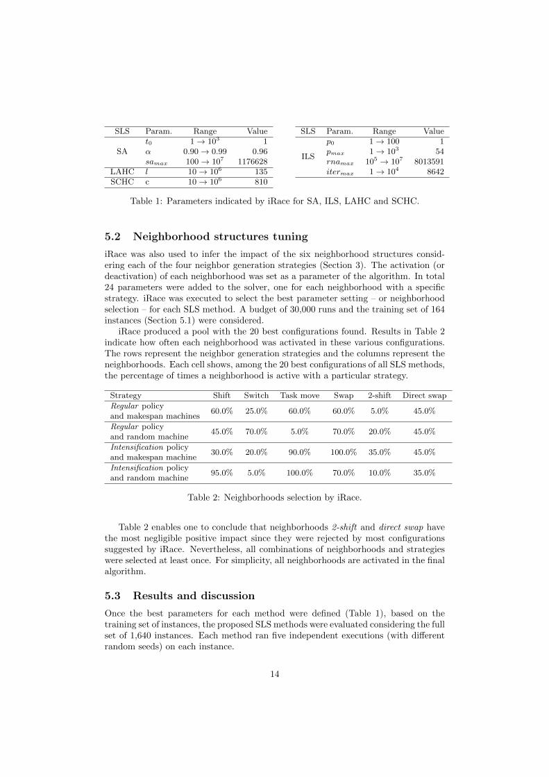
SLS Param. Range Value SLS Param. Range Value

SAt0 1→ 103 1

ILS

p0 1→ 100 1α 0.90→ 0.99 0.96 pmax 1→ 103 54samax 100→ 107 1176628 rnamax 105 → 107 8013591

LAHC l 10→ 106 135 itermax 1→ 104 8642SCHC c 10→ 106 810

Table 1: Parameters indicated by iRace for SA, ILS, LAHC and SCHC.

5.2 Neighborhood structures tuning

iRace was also used to infer the impact of the six neighborhood structures consid-ering each of the four neighbor generation strategies (Section 3). The activation (ordeactivation) of each neighborhood was set as a parameter of the algorithm. In total24 parameters were added to the solver, one for each neighborhood with a specificstrategy. iRace was executed to select the best parameter setting – or neighborhoodselection – for each SLS method. A budget of 30,000 runs and the training set of 164instances (Section 5.1) were considered.

iRace produced a pool with the 20 best configurations found. Results in Table 2indicate how often each neighborhood was activated in these various configurations.The rows represent the neighbor generation strategies and the columns represent theneighborhoods. Each cell shows, among the 20 best configurations of all SLS methods,the percentage of times a neighborhood is active with a particular strategy.

Strategy Shift Switch Task move Swap 2-shift Direct swap

Regular policyand makespan machines

60.0% 25.0% 60.0% 60.0% 5.0% 45.0%

Regular policyand random machine

45.0% 70.0% 5.0% 70.0% 20.0% 45.0%

Intensification policyand makespan machine

30.0% 20.0% 90.0% 100.0% 35.0% 45.0%

Intensification policyand random machine

95.0% 5.0% 100.0% 70.0% 10.0% 35.0%

Table 2: Neighborhoods selection by iRace.

Table 2 enables one to conclude that neighborhoods 2-shift and direct swap havethe most negligible positive impact since they were rejected by most configurationssuggested by iRace. Nevertheless, all combinations of neighborhoods and strategieswere selected at least once. For simplicity, all neighborhoods are activated in the finalalgorithm.

5.3 Results and discussion

Once the best parameters for each method were defined (Table 1), based on thetraining set of instances, the proposed SLS methods were evaluated considering the fullset of 1,640 instances. Each method ran five independent executions (with differentrandom seeds) on each instance.

14

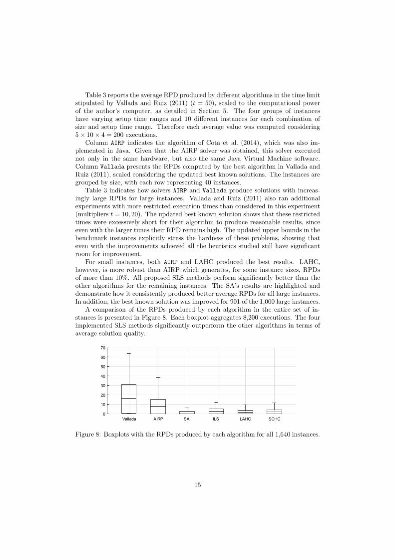
Table 3 reports the average RPD produced by different algorithms in the time limitstipulated by Vallada and Ruiz (2011) (t = 50), scaled to the computational powerof the author’s computer, as detailed in Section 5. The four groups of instanceshave varying setup time ranges and 10 different instances for each combination ofsize and setup time range. Therefore each average value was computed considering5× 10× 4 = 200 executions.

Column AIRP indicates the algorithm of Cota et al. (2014), which was also im-plemented in Java. Given that the AIRP solver was obtained, this solver executednot only in the same hardware, but also the same Java Virtual Machine software.Column Vallada presents the RPDs computed by the best algorithm in Vallada andRuiz (2011), scaled considering the updated best known solutions. The instances aregrouped by size, with each row representing 40 instances.

Table 3 indicates how solvers AIRP and Vallada produce solutions with increas-ingly large RPDs for large instances. Vallada and Ruiz (2011) also ran additionalexperiments with more restricted execution times than considered in this experiment(multipliers t = 10, 20). The updated best known solution shows that these restrictedtimes were excessively short for their algorithm to produce reasonable results, sinceeven with the larger times their RPD remains high. The updated upper bounds in thebenchmark instances explicitly stress the hardness of these problems, showing thateven with the improvements achieved all the heuristics studied still have significantroom for improvement.

For small instances, both AIRP and LAHC produced the best results. LAHC,however, is more robust than AIRP which generates, for some instance sizes, RPDsof more than 10%. All proposed SLS methods perform significantly better than theother algorithms for the remaining instances. The SA’s results are highlighted anddemonstrate how it consistently produced better average RPDs for all large instances.In addition, the best known solution was improved for 901 of the 1,000 large instances.

A comparison of the RPDs produced by each algorithm in the entire set of in-stances is presented in Figure 8. Each boxplot aggregates 8,200 executions. The fourimplemented SLS methods significantly outperform the other algorithms in terms ofaverage solution quality.

0

10

20

30

40

50

60

70

Vallada AIRP SA ILS LAHC SCHC

Figure 8: Boxplots with the RPDs produced by each algorithm for all 1,640 instances.

15

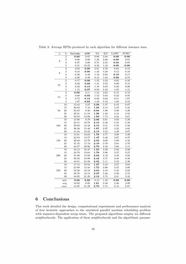
Table 3: Average RPDs produced by each algorithm for different instance sizes.

n k Vallada AIRP SA ILS LAHC SCHC

6

2 0.00 0.87 0.86 2.04 0.00 0.003 0.08 0.08 1.28 2.08 0.00 0.014 0.27 3.80 0.75 2.25 0.04 0.055 0.21 10.25 0.32 1.33 0.00 0.00

8

2 0.03 0.00 2.01 2.76 0.04 0.133 0.24 0.00 1.33 4.28 0.12 0.194 0.39 0.48 1.16 2.93 0.10 0.175 0.20 0.38 0.12 1.64 0.00 0.55

10

2 0.17 0.00 1.35 3.23 0.05 0.333 0.20 0.00 1.21 2.93 0.09 0.444 0.32 0.13 1.18 3.83 0.30 0.965 1.15 0.27 0.56 3.33 1.05 1.41

12

2 0.09 0.11 1.54 2.63 0.15 0.723 0.08 0.03 1.52 3.94 0.22 0.954 0.75 0.12 0.99 3.62 0.51 1.675 1.67 0.63 1.28 5.10 1.66 2.53

50

10 12.42 5.97 2.38 5.37 6.43 6.8715 20.83 7.10 1.58 3.14 5.33 5.3220 25.65 9.30 0.94 1.96 3.90 4.2625 30.21 11.54 1.26 1.82 4.14 4.5230 32.83 12.80 1.63 1.74 3.24 3.61

100

10 13.96 8.79 2.06 3.81 3.92 5.2015 22.41 10.78 2.15 3.48 5.34 5.4020 29.63 13.42 2.15 3.51 5.33 5.5825 36.39 15.40 1.97 2.97 4.22 4.8230 41.64 19.22 2.13 3.52 4.20 3.87

150

10 15.81 10.03 1.78 3.77 3.08 4.3915 22.83 12.57 1.47 3.46 3.67 4.3720 30.62 14.78 2.33 3.68 4.09 4.4225 37.45 17.19 2.19 3.78 3.84 3.7830 43.27 20.06 2.70 4.49 3.80 4.15

200

10 16.14 10.47 1.55 3.39 2.92 3.9815 24.76 13.64 1.78 3.96 3.37 4.2720 31.89 15.89 2.03 4.18 3.49 3.9225 39.33 18.99 2.42 4.57 3.58 3.5630 44.81 21.08 2.32 5.11 3.24 3.36

250

10 17.14 10.52 1.57 3.44 2.67 3.6415 25.09 13.44 1.72 3.98 3.25 4.0920 33.38 16.18 2.04 4.45 3.45 3.9325 39.79 19.15 2.37 5.26 3.39 3.7230 44.95 21.29 2.10 5.74 2.81 3.32

min 0.00 0.00 0.12 1.33 0.00 0.00avg 18.03 8.95 1.61 3.48 2.46 2.89max 44.95 21.29 2.70 5.74 6.43 6.87

6 Conclusions

This work detailed the design, computational experiments and performance analysisof four heuristic approaches to the unrelated parallel machine scheduling problemwith sequence-dependent setup times. The proposed algorithms employ six differentneighborhoods. The application of these neighborhoods and the algorithmic parame-

16

ters were extensively tuned, both applying a manual selection of parameters and theiRace package to automate the search for the best parameter configuration.

The proposed SLS algorithms consistently produced good results, outperformingtwo of the current best algorithms for the UPMSP when considering the solutionquality produced in restricted computation times. The bounds of 901 out of 1000large instances were improved over the previous best known solutions. All proposedalgorithms have the advantage of being much simpler to implement than recentlyproposed hybrid heuristics.

After comparing the implemented metaheuristics, one very interesting observationbecame apparent. When tuning optimization algorithms, the method with fewer pa-rameters is not necessarily the easiest to tune. For instance, Simulated Annealing(SA) has more parameters than Step Counting Hill Climbing (SCHC). However, ex-tensive tuning revealed that many different parameter configurations for SA presentedsimilarly good results. Despite the extensive set of experiments conducted, SCHC wasunable to replicate SA’s impressive results.

The results open up opportunities for future research regarding the developmentof fundamental heuristics to be applied withing SLS algorithms for scheduling andother combinatorial optimization problems. Given the unraveled correlation betweenthe number of parameters and the robustness of SLS algorithms, it is worthwhilerevising the application range of the algorithms belonging to this class.

Acknowledgements

We acknowledge FAPEMIG and CNPq for supporting the development of this re-search, as well as the Belgian Science Policy Office (BELSPO) in the InteruniversityAttraction Pole COMEX (http://comex.ulb.ac.be) and the Leuven Mobility ResearchCenter. The computational resources and services used in this work were provided bythe VSC (Flemish Supercomputer Center), funded by the Hercules Foundation andthe Flemish Government – department EWI.

References

Allahverdi, A., Ng, C., Cheng, T., Kovalyov, M. Y., 2008. A survey of schedulingproblems with setup times or costs. European Journal of Operational Research187 (3), 985–1032.

Avalos-Rosales, O., Alvarez, A. M., Angel-Bello, F., 2013. A reformulation for theproblem of scheduling unrelated parallel machines with sequence and machine de-pendent setup times. In: Twenty-Third International Conference on AutomatedPlanning and Scheduling. pp. 278–282.

Avalos-Rosales, O., Angel-Bello, F., Alvarez, A., 2015. Efficient metaheuristic algo-rithm and re-formulations for the unrelated parallel machine scheduling problemwith sequence and machine-dependent setup times. The International Journal ofAdvanced Manufacturing Technology 76 (9-12), 1705–1718.

17

Birattari, M., Balaprakash, P., Dorigo, M., 2007. The ACO/F-race algorithm for com-binatorial optimization under uncertainty. In: Doerner, K., Gendreau, M., Greis-torfer, P., Gutjahr, W., R.F., H., Reimann, M. (Eds.), Metaheuristics–Progress inComplex Systems Optimization. Operations Research/Computer Science InterfacesSeries. Springer, Berlin, Germany, pp. 189–203.

Burke, E. K., Bykov, Y., 2008. A Late Acceptance Strategy in Hill-Climbing forExam Timetabling Problems. In: PATAT ’08 Proceedings of the 7th InternationalConference on the Practice and Theory of Automated Timetabling.

Burke, E. K., Bykov, Y., 2012. The Late Acceptance Hill-Climbing Heuristic. Tech.Rep. CSM-192, Department of Computing Science and Mathematics, University ofStirling.

Bykov, Y., Petrovic, S., 2013. An initial study of a novel Step Counting Hill Climbingheuristic applied to timetabling problems. In: Kendall, G., Berghe, G. V., McCol-lum, B. (Eds.), MISTA 2013: Proceedings of the 6th Multidisciplinary InternationalConference on Scheduling: Theory and Applications. Gent, Belgium, pp. 691–693.

Cota, L., Haddad, M., Souza, M., Coelho, V., 2014. AIRP: A heuristic algorithmfor solving the unrelated parallel machine scheduling problem. In: EvolutionaryComputation (CEC), 2014 IEEE Congress on. IEEE, pp. 1855–1862.

De Paula, M. R., Ravetti, M. G., Mateus, G. R., Pardalos, P. M., 2007. Solving parallelmachines scheduling problems with sequence-dependent setup times using variableneighbourhood search. IMA Journal Management Mathematics 18 (2), 101–115.

Dueck, G., Scheuer, T., 1990. Threshold accepting: a general purpose optimizationalgorithm appearing superior to simulated annealing. Journal of computationalphysics 90 (1), 161–175.

Feo, T. A., Resende, M. G. C., 1995. Greedy randomized adaptive search procedures.In: Journal of Global Optimization. Vol. 6. Springer, pp. 109–133.

Garey, M. R., Johnson, D. S., 1979. Computers and Intractability: A Guide to theTheory of NP-Completeness. W. H. Freeman and Company.

Glover, F., Laguna, M., Martı, R., 2000. Fundamentals of scatter search and pathrelinking. Control and cybernetics 29 (3), 653–684.

Goldberg, D. E., 1989. Genetic Algorithms in Search, Optimization and MachineLearning. Addison-Wesley. Berkeley.

Graham, R., Lawler, E., Lenstra, J., Rinnooy Kan, A., 1979. Optimization and Ap-proximation in Deterministic Sequencing and Scheduling: A Survey. Annals of Dis-crete Mathematics 5 (2), 287–326.

Hansen, P., Mladenovic, N., 1997. Variable Neighborhood Search. Computers andOperations Research 24 (11), 1097–1100.

18

Henderson, D., Jacobson, S. H., Johnson, A. W., 2003. The theory and practiceof simulated annealing. In: Glover, F., Kochenberger, G. (Eds.), Handbook ofMetaheuristics. International Series in Operations Research & Management Science.Kluwer Academic Publishers, pp. 287–319.

Hoos, H. H., Stutzle, T., 2005. Stochastic Local Search: Foundations and Applica-tions. Morgan Kaufmann, Ch. Empirical Analysis of SLS Algorithms, pp. 149–201.

Kendall, G., Bai, R., B lazewicz, J., De Causmaecker, P., Gendreau, M., John, R., Li,J., McCollum, B., Pesch, E., Qu, R., Sabar, N., Vanden Berghe, G., Lee, A., 2016.Good laboratory practice for optimization research. Journal of the OperationalResearch Society 67 (4), 676–689.

Kim, D., Kim, K., Jang, W., Chen, F., 2002. Unrelated parallel machine schedulingwith setup times using simulated annealing. Robotics and Computer-IntegratedManufacturing 18 (3-4), 223–231.

Kirkpatrick, S., Gelatt, C. D., Vecchi, M. P., 1983. Optimization by simulated an-nealing. Science 220 (4598), 671–680.

Lopez-Ibanez, M., Dubois-Lacoste, J., Stutzle, T., Birattari, M., 2011. The iracepackage: Iterated racing for automatic algorithm configuration. IRIDIA, UniversiteLibre de Bruxelles, Belgium, Tech. Rep. TR/IRIDIA/2011-004.

Lopez-Ibanez, M., Stutzle, T., 2014. Automatically improving the anytime behaviourof optimisation algorithms. European Journal of Operational Research 235 (3), 569– 582.

Lourenco, H. R., Martin, O. C., Stutzle, T., 2003. Iterated local search. In: Glover,F., Kochenberger, G. (Eds.), Handbook of Metaheuristics. Kluwer Academic Pub-lishers, Boston, Ch. 11.

McConnell, S., 2004. Code complete. Pearson Education.

PassMark software, 2015. CPU benchmarks.URL https://www.cpubenchmark.net/

R Development Core Team, 2008. R: A Language and Environment for StatisticalComputing. R Foundation for Statistical Computing, Vienna, Austria.URL http://www.R-project.org

Rabadi, G., Moraga, R., Ameer, A., 2006. Heuristics for the unrelated parallel machinescheduling problem with setup times. Journal of Intelligent Manufacturing 17, 85–97.

SOA-ITI, Nov. 2013. Grupo de investigacion SOA: Sistemas de optimizacion aplicada.URL http://soa.iti.es/

Vallada, E., Ruiz, R., 2011. A genetic algorithm for the unrelated parallel machinescheduling problem with sequence dependent setup times. European Journal ofOperational Research 211 (3), 612–622.

19