Parallel stochastic line search methods with feedback for ...people.dmi.uns.ac.rs/~natasa/mainPkminMarch19.pdf · Noname manuscript No. (will be inserted by the editor) Parallel stochastic

Noname manuscript No.(will be inserted by the editor)

Parallel stochastic line search methods with feedbackfor minimizing finite sums

Dragana Bajovic · Dusan Jakovetic ·Natasa Krejic · Natasa Krklec Jerinkic

Received: date / Accepted: date

Abstract We consider unconstrained minimization of a finite sum of N con-tinuously differentiable, not necessarily convex, cost functions. Several gradient-like (and more generally, line search) methods, where the full gradient (thesum of N component costs’ gradients) at each iteration k is replaced withan inexpensive approximation based on a sub-sample Nk of the componentcosts’ gradients, are available in the literature. However, a vast majority ofthe methods considers pre-determined (either deterministic or random) rulesfor selecting subsets Nk; these rules are unrelated with the actual progressof the algorithm along iterations. In this paper, we propose a very generalframework for nonmonotone line search algorithms with an adaptive choice ofsub-samplesNk. Specifically, we consider master-worker architectures with onemaster and N workers, where each worker holds one component function fi.The master maintains the solution estimate xk and controls the states of theworkers (active or inactive) through a single scalar control parameter pk. Eachactive worker sends to the master the value and the gradient of its compo-

Dragana BajovicBiosense Institute, University of Novi SadZorana Djindjica 3, 21000 Novi Sad, SerbiaE-mail: [email protected]

Dusan JakoveticDepartment of Mathematics and Informatics, Faculty of Sciences, University of Novi SadTrg Dositeja Obradovica 4, 21000 Novi Sad, SerbiaE-mail: [email protected]

Natasa KrejicDepartment of Mathematics and Informatics, Faculty of Sciences, University of Novi SadTrg Dositeja Obradovica 4, 21000 Novi Sad, SerbiaE-mail: [email protected]

Natasa Krklec JerinkicDepartment of Mathematics and Informatics, Faculty of Sciences, University of Novi SadTrg Dositeja Obradovica 4, 21000 Novi Sad, SerbiaE-mail: [email protected]

2 Dragana Bajovic et al.

nent cost, while inactive workers stay idle. Parameter pk is proportional tothe expected (average) number of active workers (which equals the averagesample size), and it can increase or decrease along iterations based on a com-putationally inexpensive estimate of the algorithm progress. Hence, throughparameter pk, the master sends feedback to the workers about the desiredsample size at the next iteration. For the proposed algorithmic framework, weshow that each accumulation point of sequence {xk} is a stationary point ofthe full cost function, almost surely. Simulations on both synthetic and realworld data sets illustrate the benefits of the proposed framework with respectto the existing non-adaptive rules.

Key words: Variable sample methods; Stochastic optimization; Parallelalgorithms; Non-convex cost functions; Feedback.

1 Introduction

We consider problems of the form:

minx∈Rn

f(x) :=1

N

N∑i=i

fi(x), (1)

where each fi : Rn → R, i = 1, ..., N, is a continuously differentiable (notnecessarily convex) function. Such problems arise frequently in machine learn-ing, where a (usually large scale sized) training data set is partitioned into Nsubsets, and each fi represents a loss with respect to each of the training datasubsets. (Note that usually fi here is itself a sum over the individual trainingdata examples but this is abstracted here.)

In the scenarios of large training sets, it can be beneficial to apply gradient-like methods, where the full gradient (gradient of f) at each iteration k is re-placed with an inexpensive estimate. Usually, the estimate of ∇f(xk) (xk ∈ Rn

being the current iterate) is of the form: 1|Nk|

∑i∈Nk

∇fi(xk), where Nk is a

subset of N = {1, ..., N}. Therefore, in a sense, instead of working with thefull cost function f , such algorithms work at each iteration k with a less in-expensive, but inexact version fNk

:= 1|Nk|

∑i∈Nk

fi. The algorithms of this

type include incremental [5,23], stochastic [33,41,30,38,24], and hybrid meth-ods [13]. Besides the gradient approximations, they can also utilize differentsearch directions (generated according to the available information – the avail-able subset Nk), including, e.g., Quasi-Newton-type directions, e.g., [13,19].Indeed, [9] demonstrate the benefits of employing the limited-memory BFGSand similar rules in the context of variable sample size methods for solvingproblems of form (1).

The existing literature mainly considers pre-determined (deterministic orrandom) rules for selecting subsets Nk. These rules are oblivious to the actualalgorithm progress at specific iterations. In other words, the algorithm selects(possibly random) samples Nk’s independently from the current iterate xk andindependently from the estimated progress at the current iteration k.

Parallel stochastic line search methods with feedback for minimizing finite sums 3

Variable sample size approach or adaptive scheduling schemes have alsobeen considered for solving problems of type (1). Reference [15] considers thecase of convex stochastic optimization and derives error bounds in terms ofsample size, similar to the results in [36] for the strongly convex case. A re-lationship between the sample size growth and the deterministic convergencerate for a class of optimization methods is considered in [26,27]. A set ofconditions that ensures almost sure convergence is presented in [27], togetherwith a specific recommendation for sample size and error tolerance sequences.Another interesting approach that offers a quantitative measure of a solu-tion quality is presented in [31]. Optimality functions for general stochasticprograms (expected value objective and constraint functions) are consideredand an algorithm that utilizes optimality functions to select sample size isdeveloped. An adaptive sample size scheduling is considered in [17] as well.Different types of stochastic equilibrium problems and applications of vari-able sample size schemes are the topic of study in [37]. Furthermore, variablesample scheduling for second order methods is employed in [8,9]. A review ofvariable sample size methods is available in [20].

In this paper, building from references [2–4] and the prior work [18,19], wepropose a framework for nonmonotone line search methods with an adaptivechoice of the sets Nk. We consider the commonly used master-worker model,e.g., of computing machines in a cluster, with one master node and N workernodes; see, e.g., [1,21,7,39,34], for similar models. Each worker i holds onefunction fi in (1) and can evaluate this function’s values and its gradients.This model is adequate for large-scale distributed optimization in cluster orcloud environments, whereby the training data set at each worker i – whichparameterizes function fi – is so large that it is infeasible to transfer norstore all the workers’ data at the master; or, in alterative, the workers cannotsend their data to the master due to privacy constraints (while the variabledimension n and the number of nodes N are of a moderate to medium size.)

The master node coordinates computation and updates the solution es-timate xk ∈ Rn (see Figure 1). Each worker, at each iteration k, can bein two possible states: active and inactive. Active workers i compute pairs(fi(xk), ∇fi(xk)) and send them to the master, while inactive workers stayidle. The state of each worker, and therefore the (average) size of the sam-ple Nk, is controlled by the master, and it is increased or decreased as needed,based on the actual progress of the algorithm. Therefore, the algorithm in-corporates feedback information from the master to the workers about what(average) sample size is needed for efficient progress at the next iteration. Theproposed framework considers a nonmonotone line search, and it is flexiblewith respect to the utilized search directions – we allow for arbitrary directionswhich are descent with respect to the available function approximation fNk

.

In more details, at each iteration k, the master node broadcasts to allworkers the current estimate xk and a control parameter pk ∈ [0, 1]. Uponreception of pk, each worker i decides, independently from other workers butdependently upon its previous state (see Section 2 for details), whether it willbe active at iteration k; it becomes active with probability pk (in which case


it evaluates the pair (fi(xk), ∇fi(xk)) and transmits it to the master) andinactive with probability 1−pk (in which case it stays idle). Hence, the masterworks with a sample of an average size N pk, updates xk via a nonmonotoneline search rule, and it decides on the value of the next control parameter pk+1;the latter quantity can either decrease, stay equal, or increase with respectto pk. The update rule for the control parameter pk is based on the comparativesize of two quantities, which we denote by dmk and εk. The quantity dmk is asuitable measure of progress made with respect to the current function fNk

; thequantity εk estimates how different fNk

is with respect to the true objective fat the current iterate xk. The adaptive rule for choosing pk operates as follows.If dmk is small relative to εk, pk+1 increases with respect to pk. Intuitively,the progress which is possible based on the average sample size equal to N pkis exhausted, and hence the precision of approximating f should be increased.Conversely, if dmk is large with respect to εk, then pk+1 is decreased withrespect to pk. Intuitively, the progress can still be achieved even with a lowerprecision, and hence the average sample size is decreased. The change (increaseor decrease) in pk is set such that the quantities dmk and εk are kept in abalance (i.e., they have comparable values) across iterations.

Our main results are as follows. Assuming that the fi’s are continuouslydifferentiable and bounded from below (and not necessarily convex), we showthat, eventually (starting from a finite iteration), the master works with thefull sample (pk = 1), almost surely. This eventual involvement of all workers inthe optimization process, i.e., the achievement of the “full precision,” is not ar-tificially enforced in the algorithm, but is rather a result of a carefully designedfeedback process between the master and the workers. Moreover, we show thatevery accumulation point of the sequence of iterates {xk} is a stationary pointof the desired cost function f . Simulation examples on quadratic and logisticlosses, both on artificial and real world data sets, demonstrate that the pro-posed method incurs significant savings in the total number of function andgradient evaluations with respect to existing alternatives which do not incor-porate feedback – specifically the methods where the true objective function(and its gradient) is used at all iterations, and the hybrid (incremental) schemein [13].

Therefore, the purpose of the current paper is to introduce the proposedadaptive framework, establish convergence guarantees to a stationary pointunder very generic, not necessarily convex, costs, and deliver initial numericalresults.

This paper builds on references [2–4] and [18,19] for centralized optimiza-tion. In [2–4], the authors propose an algorithm which allows that the samplesize both increase and decrease along iterations within the trust region frame-work. A similar mechanism for the schedule sequence in a line search frameworkis developed in [18]. Reference [19] extends the work in [18] to a nonmonotoneline search framework. In this paper, we also consider a nonmonotone linesearch framework, as done in [19]. However, a major difference of the currentpaper with respect to [19] and [2–4,18] is that here the sample size is con-trolled only in terms of its mean value, and not in terms of the actual current


size. From the implementation perspective, the framework proposed here ismuch more suitable for, e.g., cluster environments, as the master controls thecurrent sample through a single scalar parameter pk, which it broadcasts toall workers. In contrast, with the algorithms in [2–4,18,19], the master needsa more complex control mechanism, for example to contact each of the work-ers individually and declare each of them active or inactive. Finally, from theperspective of the algorithm design and analysis, the simplified sample sizecontrol here corresponds to a more challenging situation in the design of thecontrol rules and the algorithm analysis. Specifically, compared with [19] – thework closest to this paper – we introduce here a very different lower boundfor controlling the pk’s which is essential to ensure eventual activation of allworkers and hence the convergence to a stationary point.

Paper organization. Section 2 describes the model that we assume andpresents the proposed algorithmic framework, while Section 3 provides its con-vergence analysis. In Section 4 we present the results of the initial numericaltestings. Finally, in Section 5, some conclusions about the proposed frameworkare drawn.

2 Model and algorithm

We consider a master-worker computational model (Figure 1); see also [1,21,7,39,34]. Each worker i holds a continuously differentiable, not necessarilyconvex, function fi : Rn → R, i = 1, ..., N . Unlike, e.g., [13], we do not imposeany assumptions on the “similarity” among the fi’s; that is, we do not requirethat the minimizers of the individual fi’s – if they exist – are close or withina pre-defined distance from each other. This allows, for example, that thetraining data sets from different workers may be generated from very differentdistributions.

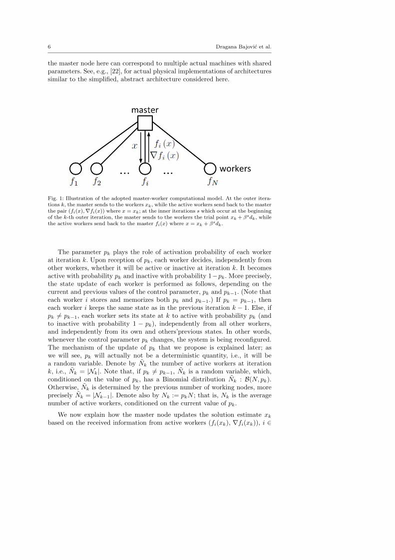
The master-worker system solves problem (1) through an iterative algo-rithm, as follows. The algorithm consists of the outer iterations k and theinner iterations s. We first describe the outer iterations k.1 The master nodemaintains over k the solution estimate xk ∈ Rn. At each iteration k, the mas-ter node broadcasts to all workers quantity xk and a scalar control parameterpk ∈ [0, 1]. At each iteration k, each worker can be in one of the two pos-sible states: active and inactive. As we will see further ahead, the state ofeach worker does not change along the inner iterations. Each active worker icalculates the pair (fi(xk), ∇fi(xk)) and sends it back to the master.

The assumed abstract master-worker architecture is well suited for situ-ations where the variable dimension n and the number of nodes N are of amoderate to medium size, while each fi may correspond to a large-sized train-ing data set, so that it is economical that each worker stores and keeps locallythis training data, calculates locally the pair (fi(xk), ∇fi(xk)), and then com-municates the pair with the master. Note that the physical implementation of

1 From now on, we refer to the outer iterations simply as iterations.


the master node here can correspond to multiple actual machines with sharedparameters. See, e.g., [22], for actual physical implementations of architecturessimilar to the simplified, abstract architecture considered here.

Fig. 1: Illustration of the adopted master-worker computational model. At the outer itera-tions k, the master sends to the workers xk, while the active workers send back to the masterthe pair (fi(x),∇fi(x)) where x = xk; at the inner iterations s which occur at the beginningof the k-th outer iteration, the master sends to the workers the trial point xk + βsdk, whilethe active workers send back to the master fi(x) where x = xk + βsdk.

The parameter pk plays the role of activation probability of each workerat iteration k. Upon reception of pk, each worker decides, independently fromother workers, whether it will be active or inactive at iteration k. It becomesactive with probability pk and inactive with probability 1−pk. More precisely,the state update of each worker is performed as follows, depending on thecurrent and previous values of the control parameter, pk and pk−1. (Note thateach worker i stores and memorizes both pk and pk−1.) If pk = pk−1, theneach worker i keeps the same state as in the previous iteration k − 1. Else, ifpk 6= pk−1, each worker sets its state at k to active with probability pk (andto inactive with probability 1 − pk), independently from all other workers,and independently from its own and others’previous states. In other words,whenever the control parameter pk changes, the system is being reconfigured.The mechanism of the update of pk that we propose is explained later; aswe will see, pk will actually not be a deterministic quantity, i.e., it will bea random variable. Denote by Nk the number of active workers at iterationk, i.e., Nk = |Nk|. Note that, if pk 6= pk−1, Nk is a random variable, which,conditioned on the value of pk, has a Binomial distribution Nk : B(N, pk).Otherwise, Nk is determined by the previous number of working nodes, moreprecisely Nk = |Nk−1|. Denote also by Nk := pkN ; that is, Nk is the averagenumber of active workers, conditioned on the current value of pk.

We now explain how the master node updates the solution estimate xkbased on the received information from active workers (fi(xk), ∇fi(xk)), i ∈


Nk, i.e., based on the function

fNk(x) =

1

|Nk|∑i∈Nk

fi(x).

Specifically, the subsequent solution estimate is obtained through a nonmono-tone line search rule with generic descent directions, as follows:

xk+1 = xk + αkdk,

where dk is the search direction and αk is the step size. We allow for a genericdescent search direction dk for function fNk

, i.e., dk is such that

dTk∇fNk(xk) < 0.

We now discuss some practical possibilities for the choice of dk. The obviouschoice is dk = −∇fNk

(xk). However, incorporating some second order infor-mation can enhance the algorithm significantly, especially if the nonmonotoneline search rule is applied as suggested below. For example, one can employthe spectral gradient direction of the form dk = −zk∇fNk

(xk), where zk is apositive constant obtained trough xk − xk−1 and ∇fNk

(xk)−∇fNk−1(xk−1),

see, e.g., [6] for details. In this case, the master node has to store the previoussolution estimate xk−1 and the previous gradient ∇fNk−1

(xk−1) in order tocalculate the new search direction; that is, it additionally stores two vectorsof length n. In alternative, one can use Quasi-Newton types of directions suchas BFGS. Such directions are of the form dk = −Hk∇fNk

(xk), where Hk isupdated via an inexpensive recursion, such that positive definiteness of Hk ismaintained. Overall, compared with the spectral gradient method, the masteradditionally stores an n× n matrix and performs its update over iterations k.Finally, when the memory requirements for BFGS are an issue, one can con-sider the limited memory BFGS approach as suggested in [8,9].

We now describe the inner iterations s; their purpose is to determine thestep size αk via an Armijo-type rule. Specifically, once the master calculates dk,it initiates the inner iterations s = 0, 1, ... At each s, the master evaluates atrial point xk+βs dk and sends it to all the workers. The workers do not changetheir state during the inner iterations, i.e., during all inner iterations they stayin their current state. Upon reception of the trial point xk +βs dk, each activeworker i, i ∈ Nk, calculates the function value fi (xk + βsdk) and sends it backto the master. The process is repeated until the following condition is met fora certain inner iteration s (here αk := βs):

fNk(xk + αkdk) ≤ fNk

(xk) + ηαkdTk∇fNk

(xk) + ek. (2)

In (2), {ek}k∈N0is a positive (predetermined) and summable sequence,

ek > 0,

∞∑k=0

ek < e <∞. (3)


In general, this nonmonotone line search with backtracking allows for longerstep sizes when compared with the Armijo rule (wherein ek = 0). In otherwords, less trial points are needed and we expect less function evaluationsfNk

(xk + αdk) to be calculated. Besides this rule – which originates in [14] –other nonmonotone schemes like, e.g., [40], [11] [16], can also be considered,since the convergence results hold with technical differences in the proofs. Theresults obtained in a similar variable sample scheme framework [19] indicatethat the best choice for the line search rule depends on a search direction tobe used. For instance, the negative gradient search direction seems to workbetter with less freedom in (2), so the parameter ek for this direction shouldbe modest.

The proposed line search is well defined, i.e., it terminates after a finitenumber of inner iterations if the function fNk

is continuously differentiable, asassumed throughout this paper. Moreover, using backtracking makes the stepsize not too small and is considered a good substitute for the Wolfe conditions(see [25] for instance).

We now explain how the master updates the control parameter and sets thenew value pk+1. The update is governed by the actual progress of the algorithmestimated by computationally inexpensive means – this is the feature of ourwork which distinguishes it from most of the literature. Specifically, the controlparameter is updated by comparing two measures of progress: dmk and εk.The first measures the progress in decreasing the objective function and isdefined by

dmk = −αkdTk∇fNk

(xk). (4)

Some other choices of dmk ≥ 0 are possible as well (see [19] for details)but are not considered in this paper. The purpose of the second measure ofprogress εk, is to estimate the error which is generated by employing the sampleaverage function fNk

instead of f . The quantity εk = εk(p) is a function ofthe next control parameter p = pk+1 which is to be determined; εk(p) mayalso depend on the data currently available at the master, e.g., on the valuefNk

(xk) - this is encoded in the subscript k of notation εk(p). The functionp 7→ εk(p) can be very generic. As it can be seen from the proofs, the onlytechnical requirement is that εk(p) ≥ 0 for all p ∈ [0, 1] and bounded awayfrom zero for all p ∈ [0, 1). However, a desirable property is that εk(p) is adecreasing function with respect to p.

Let us now discuss the specific choices of p and εk(p). We assume that thecontrol parameter pk takes values from the discrete set Π = {π1, π2, ..., πm},where 0 < π1 < π2 < ... < πm = 1. The number of allowed values (m) can bearbitrary large. However, our tests indicate that m ≤ N provides sufficientlygood performance. Regarding εk(p), one possibility is to set εk(p) = 1 − p,which is feasible as we assume that p can take only finitely many discretevalues. This is a simple choice which is easy to calculate, but it does not accountfor the influence of the current solution estimate xk. In order to incorporate


the latter information, one can define

εk(p) = µσk√pN

, (5)

where µ is a positive constant and σ2k measures the variance (spread) of the

set of values fi(xk), i ∈ Nk and is defined by

σ2k =

1

|Nk|∑i∈Nk

(fi(xk)− 1

|Nk|fNk

(xk)

)2

. (6)

Regarding the update of the control parameter, the main idea is to con-struct an algorithm that allows us to work with as few nodes as we can andstill ensure continuous progress over iterations k, especially at the beginning ofthe optimization process. However, in order to ensure almost sure convergencetowards a stationary point of the true objective function f , we need to reachthe whole set of nodes eventually. There are two crucial points which makethis possible. One of them is incorporated in step S3 of the main algorithm(see ahead Algorithm 3), and it states that the set of active nodes does notchange if the control parameter remains the same. As it can be seen from theproofs, this requirement discards the scenario where pk = p = const < 1 for allk large enough. On the other hand, persistent oscillations of active nodes haveto be avoided. This is achieved by a safeguard sequence denoted by {pmin

k }.This sequence will be a lower bound for the true probability parameter pk,i.e., it will be required that pk+1 ≥ pmin

k for all k. The update of this safeguardsequence will be described later on.

Let the lowest allowed probability π1 define the initial safeguard pmin0 := π1

and take this value as the initial probability, i.e. p0 := pmin0 . In order to perform

the update of the safeguard pmink , the master has to store and update a vector

of length m which is denoted by Fk = ([Fk]1, ..., [Fk]m). The role of this vector,is to track the approximate objective function values for different values of pk,i.e., for different precision levels. The jth component [Fk]j corresponds tothe precision level controlled by πj and represents the lowest value of theapproximate objective function defined by πj precision level achieved withinthe first k iterations. Recall that the control parameter determines only theexpected number of working nodes. Therefore, Fk tracks different levels of theexpected precision. Each component of this vector is initially set to +∞. It isworth noting that our theory allows that m can be taken independently fromN . Hence, when N grows very large, m can be chosen so that it stays boundedas N grows; therefore, storing and maintaining Fk does not induce significantcosts.

The algorithm for updating the lower bound pmink is presented below. The

main idea is to increase the lower bound, and therefore increase the expectedprecision, if there was not enough decrease in the approximate objective func-tion fNk

. More precisely, we track the decrease of the expected precision leveldetermined by pk+1 which is to be used in the following iteration. Beforestating the algorithm, we introduce parameters θk and γk which determine


sufficient decrease in the approximate objective function and increase in thelower bound, respectively. They are both generic parameters assumed only tobe positive and uniformly bounded away from zero. Further details on suitablechoices of these parameters are given in Section 4, and the algorithms beloware stated with generic values.

The updating of the lower bound pmink at the master is stated within Al-

gorithm 1 below. Note that the sequence {pmink }k∈N is nondecreasing and

bounded from above by 1.

ALGORITHM 1.

Updating the lower bound pmink at the master

S0 Input parameters: pk, pk+1, fNk+1(xk+1), fmin

k , θk, γk.Let j be such that πj = pk+1.

S1 Updating the lower bound.If pk < pk+1 and [Fk]j − fNk+1

(xk+1) < θk set

pmink+1 = min{1, pmin

k + γk}.

Else, pmink+1 = pmin

k .S2 Updating vector Fk

If pk < pk+1, set

[Fk+1]j = min{fNk+1(xk+1), [Fk]j}.

Else, Fk+1 = Fk.

Notice that if pk+1 is used for the first time then [Fk+1]j = ∞ and thelower bound remains unchanged. Also, recall that the number of active nodes|Nk+1| does not have to be equal to Nk+1.

Now, let us state the algorithm for updating the control parameter pkand the main algorithm. These algorithms are presented with generic searchdirections, generic function εk and generic parameters θk, γk. The algorithmsallow a lot of freedom in choosing these quantities. In Section 4 we state thespecific parameter values used in the initial numerical testings with the BFGSsearch direction. The almost sure convergence is proved in Section 3 underrather general assumptions. Furthermore, our initial tests indicate that thesafeguard lower bounds pmin

k do not significantly affect the actual update ofthe control parameter pk and thus their role is just to provide a theoreticalsafeguard needed for the convergence proofs.

ALGORITHM 2.

Updating the control parameter pk at the master

S0 Input parameters: dmk, pmink , pk, εk(pk), ν1 ∈ (0, 1).

S1 If pk ≤ pmink set pk+1 = min{πj ∈ Π : πj ≥ pmin

k }. Else, go to step S2.S2 1) If dmk = εk(pk) set pk+1 = pk.


2) If dmk > εk(pk) set pk+1 = max{πj ∈ Π : pmink ≤ πj ≤ pk, dmk ≤

εk(πj)}. If such pk+1 does not exist, set pk+1 = min{πj ∈ Π : πj ≥pmink }.

3) If dmk < εk(pk) andi) dmk ≥ ν1εk(pk) set pk+1 = min{πj ∈ Π : πj ≥ pk, dmk ≥ εk(πj)}.

If such pk+1 does not exist set pk+1 = 1.ii) dmk < ν1εk(pk) set pk+1 = 1.

The main idea of Algorithm 2 is to keep the two measures of precisionclose to each other by adapting the expected precision level. If dmk > εk(pk),the precision is too high and hence we decrease it by decreasing the controlparameter, if the lower bound pmin

k allows. Roughly speaking, the solution isstill far away and we want to approach it with smaller cost, i.e., with a smallernumber of workers activated. On the other hand, if the measure of progressin the objective function dmk is relatively small, we increase the expectedprecision by increasing the control parameter. The proposed algorithms aimto activate the whole set of nodes eventually, but only when the solutionneighborhood is approached.

The proposed overall main algorithm is given in Algorithm 3. Note thatalgorithm Algorithm 3 operates in such a way that each worker updates thestep length in coordination with the other workers, the master being in chargeof computing the search direction and updating the step length at each inneriteration of the line search.

ALGORITHM 3.

The main algorithm

S0 Input parameters at the master: pmin0 ∈ (0, 1), x0 ∈ Rn, β, ν1, η ∈ (0, 1).

S1 The master sets p0 = pmin0 and sends x0 and p0 to all the workers.

S2 Each worker activates with probability p0, independently from other work-ers. Each active worker i sends the pair (fi(x0), ∇fi(x0)) to the master.The master sets k = 0

S3 The master calculates the search direction dk such that dTk∇fNk(xk) < 0.

S4 Nonmonotone line search through inner iterations: Find the smallest non-negative integer sk such that αk = βsk satisfies

fNk(xk + αkdk) ≤ fNk

(xk) + ηαkdTk∇fNk

(xk) + ek.

At each s = 0, 1, ..., sk, the master sends xk + βsdk to all active workers,and each active worker sends back fi(xk + βsdk) to the master.

S5 The master sets xk+1 = xk + αkdk and dmk = −αkdTk∇fNk

(xk).S6 The master determines pk+1 via Algorithm 2 and sends pk+1 and xk+1 to

all the workers.S7 Workers state update: If pk+1 = pk, each worker stays in its previous

state, i.e., Nk+1 = Nk. Else, each worker activates with probability pk+1,independently from other workers, and independently from its previousstates and the previous states of other workers. The set Nk+1 consists ofthe current active nodes.


S8 Each active worker i sends the pair (fi(xk+1), ∇fi(xk+1)) to the master.S9 The master determines pmin

k+1 via Algorithm 1.S10 The master sets k = k+ 1. If Nk = N and ∇fNk

(xk) = 0, stop. Else go tostep S3.

Note from step S10 that we assumed that the master is aware of the totalnumber of workers N .

3 Convergence analysis

In this section, we prove the almost sure convergence of Algorithm 3 to astationary point of (1). Before stating this main result, we prove that, aftera finite but random number of iterations q, all nodes remain activated forall k ≥ q, almost surely. In order to prove this important intermediate result,we need the following standard assumption.

A 1. Each function fi : Rn → R, i ∈ N , is continuously differentiable andbounded from below.

Note that Assumption A1 implies that the objective function f is alsocontinuously differentiable and bounded from below.

Recall that the sequence {ek}k∈N in (2) is assumed to satisfy (3). Thequantity εk(pk) is bounded away from zero for all pk < 1. More precisely,there exist constants κ > 0 and n1 ∈ N such that εk(pk) ≥ κ for every k ≥ n1

whenever pk < 1. Even in the case where the sample variance estimate in (5)is employed, this assumption is not too restrictive since we do not expect thevariance to converge to zero. However, a positive constant can be added toεk in (5) as a safeguard, if necessary. The parameters θk and γk are boundedaway from zero, i.e., there exist constants θ > 0 and γ > 0 such that θk ≥ θand γk ≥ γ for every k.

In the following theorem we prove that control parameter pk eventuallyreaches 1. This is the crucial result for convergence analysis. The proof containstwo main arguments. First, we show that pk cannot remain at a constant valuestrictly smaller than 1 from a certain iteration onwards. Second, we show thatpk cannot exhibit persistent oscillations. Regarding the first argument, theproof given here is along the lines of the proof of Lemma 4.1 in [18]. Regardingthe second argument, the stochastic nature of the activation sets Nk hererequires a different analysis with respect to [18]. Note that a different updateof lower bounds pmin

k is used here. This second argument is the main technicalcontribution of Theorem 31.

Theorem 31. Let assumption A1 hold. Then, Algorithm 3 either terminatesafter a finite number of iterations with a stationary point of the objective func-tion f , or there exists q ∈ N such that pk = 1 for every k ≥ q.

Proof. According to step S10, the main algorithm terminates only if∇f(xk) =0. Therefore, we consider the case where the number of iterations is infinite.First, we prove that pk cannot be constant if it is strictly smaller than 1.


Recall that n1 is such that εk(pk) ≥ κ > 0 for every k ≥ n1 wheneverpk < 1. Suppose that there exists n2 > n1 such that for every k ≥ n2

pk = p1 < 1.

In that case, step S7 of Algorithm 3 implies that Nk = N 1 for every k ≥ n2 forsome fixed set N 1. Denoting gNk

k = ∇fNk(xk), we know that for every k ≥ n2

fN 1(xk+1) ≤ fN 1(xk) + ηαk(gN1

k )T dk + ek,

i.e. for every q ∈ N

fN 1(xn2+q) ≤ fN 1(xn2+q−1) + ηαn2+q−1(gN1

n2+q−1)T dn2+q−1 + en2+q−1 ≤ ...

≤ fN 1(xn2) + η

q−1∑j=0

(αn2+j(g

N 1

n2+j)T dn2+j + en2+j−1

). (7)

Now, assumption A1 implies the existence of a constant MF such that

−ηq−1∑j=0

αn2+j(gN 1

n2+j)T dn2+j ≤ fN 1(xn2)−fN 1(xn2+q)+

q−1∑j=0

en2+j ≤ fN 1(xn2)−MF +e.

(8)The inequality (8) is true for every q so

0 ≤∞∑j=0

−αn2+j(gN 1

n2+j)T dn2+j ≤

fN 1(xn2)−MF + e

η:= C.

Therefore

limk→∞

dmk = limj→∞

−αn2+j(∇fN 1(xn2+j))T dn2+j = 0. (9)

Since ν1εk(pk) ≥ ν1κ > 0 for every k ≥ n2, there exists n3 > n2 such thatdmn3

< ν1εn3(pn3

) and therefore Algorithm 2 implies pn3+1 = 1 which is incontradiction with the current assumption.

We have just proved that the probability parameter can not stay on p1 < 1.Therefore, the remaining two possible cases are as follows:

L1 There exists n4 such that pk = 1 for every k ≥ n4.L2 The sequence of probability parameters oscillates.

If the lower bound of control parameter achieves 1 at some finite iterationthen we obtain the scenario L1. Therefore, suppose that pmin

k < 1 for all k.This means that pmin

k is increased only at finitely many iterations. Therefore,based on Algorithm 1, we conclude that there exists an iteration n5 such thatfor every k ≥ n5 we have one of the following possibilities:

M1 pk+1 ≤ pk;M2 pk+1 > pk and [Fk]j(k) − fNk+1

(xk+1) ≥ θk, where pk+1 = πj(k);M3 pk+1 > pk and pk+1 has not been used before.


Now, let p = πj be the maximal probability that is used at infinitely manyiterations. Furthermore, define the set of iterations K1 at which the samplesize changes to p. The definition of p implies that there exists n6 such that forevery k ∈ K1, k ≥ n6 the probability is increased to p, i.e.

pk < pk+1 = p = πj , k ≥ n6.

Define r = max{n5, n6} and set K2 = K1

⋂{r, r + 1, . . .}. Clearly, each itera-

tion in K2 excludes the case M1. Moreover, taking out the first member of asequence K2 and retaining the same notation for the remaining sequence wecan exclude the case M3 as well. This leaves us with M2 as the only possiblescenario for iterations in K2. Therefore, for every k ∈ K2 the following is true

[Fk]j − fNk+1(xk+1) ≥ θk ≥ θ.

The number of subsets of the whole set of nodes is finite. Therefore, thereexists a subset N which appears infinitely many times within K2. So, defineK3 ⊆ K2 such that for every k ∈ K3

Nk+1 = N .

Denote K3 = {l(k)− 1}k∈N.Then for arbitrary k ∈ N we have

[Fl(k)−1]j − fN (xl(k)) ≥ θ.

Consider fN (xl(k−1)). According to the definition ofK3 we know that fN (xl(k−1))is used in step S2 of Algorithm 1 for updating [Fl(k)−1]j . Therefore,

fN (xl(k−1)) ≥ [Fl(k)−1]j

and, for every k ∈ N

fN (xl(k−1))− fN (xl(k)) ≥ θ.

However, this implies that fN is decreased for a positive constant infinitelymany times, which is in contradiction with the assumption A1. From every-thing above, we conclude that the only possible scenario is in fact L1, i.e. thereexists iteration n4 such that pk = 1 for every k ≥ n4. �Remark. It is important to notice here that in Theorem 31 q is a randomvariable, which is finite almost surely. Therefore, the value that q takes dependson a particular sample realization of the random sequence Nk and may bedifferent in each particular run of the optimization procedure.

Under the conditions stated in Theorem 31, one can easily prove the fol-lowing statement.

Theorem 32. Let assumption A1 hold. Then, Algorithm 3 either terminatesafter a finite number of iterations with a stationary point of the objective func-tion f, or there exists q ∈ N such that pk = 1 for every k ≥ q and the sequence{xk}k≥q almost surely belongs to the level set

L = {x ∈ Rn | f(x) ≤ f(xq) + e},

where e is given in (3).


In order to prove the main theorem, we need the following assumption onthe search directions.

A 2. The sequence of search directions {dk}k∈N is bounded and satisfies thefollowing implication for any subset of iterations K

limk∈K

dTk∇f(xk) = 0 ⇒ limk∈K∇f(xk) = 0

The implication in assumption A2 is satisfied for the choice dk = −∇fNk(xk).

It is also satisfied for a Quasi-Newton direction which retains positive definiteinverse Hessian approximation. The sequence of search directions is bounded,e.g., if the level set L is compact (see Theorem 3.2); this is true if, e.g., f isconvex and coercive (f(x)→ +∞ whenever ‖x‖ → +∞).

Under the additional assumption A2, the main result on the convergence ofAlgorithm 3 to a stationary point of f can be proved. We omit the argumentswhich relay on standard analysis of deterministic line search methods. Formore details, see [18] for example.

Theorem 33. Let assumptions A1-A2 hold. Then, the sequence {xk} gener-ated by Algorithm 3 is either unbounded or every accumulation point of thesequence is almost surely stationary for function f.

Proof. We have already showed that the main algorithm terminates at xk onlyif ∇f(xk) = 0. Therefore, we consider the case where the number of iterationsis infinite. In that case, Theorem 31 implies the existence of k such that pk = 1for every k ≥ k. This means that Nk = N almost surely for every k ≥ k. Thisfurthermore implies that fNk

(x) = fN (x) = f(x) almost surely for every klarge enough. Therefore, the algorithm reduces to a deterministic nonmonotoneline search algorithm on f , and hence the result follows by standard analysis.�

Clearly, Theorem 33 implies that, whenever the fi’s are in addition convex,coercive and problem (1) is solvable, then every accumulation point of thesequence {xk}k∈N generated by Algorithm 3 is a solution to (1).

4 Numerical results

The main motivation behind the proposed algorithm is to show that the class ofproblems considered in this paper can be solved with reduced communicationand computational costs and still provide an approximate solution of the samequality as if all the workers are constantly active. In order to demonstrate thebenefits of the proposed feedback approach – abbreviated here the VSS-F – it iscompared with the Sample Average Approximation method (SAA) which usesthe whole set of workers at every iteration (Nk = N for every k). Moreover, inorder to demonstrate that the feedback that controls the sample size in VSS-Fcan also provide some savings compared with the predetermined sequences ofsample sizes, we also compare VSS-F with the heuristic scheme (referred hereto as HEUR) tested in [13] where the (expected) sample size is increased by


10% at each iteration, i.e., pk+1 = min{1.1pk, 1}. Note that we set the valueof the augmentation parameter to 1.1, as used in [13]. This may not be theoptimal value, and it may be possible to tune it better for specific problems andspecific problem instances; this tuning is out of this paper’s scope. Nonetheless,the comparisons we carry out are fair as, with each of the three tested methods(including the proposed VSS-F) – we use reasonable (but ad hoc) choices ofthe tuning parameters which are kept the same across all the tested problemsand across all problem instances.

We compare the methods with respect to several criteria. The first is thenumber of function fi evaluations (FEV), where every component of the gra-dient ∇fi is counted as one function evaluation. More precisely, the cost ofcalculating fNk

(x) and ∇fNk(x) is |Nk| and n|Nk|, respectively. The total

count of FEVs includes both inner and outer iterations. This is a standardmetric for the overall computational cost of the tested methods.

Besides FEVs, we introduce the following comparison of the methods, ac-counting for the parallel architecture of the underlying computational system;see, e.g., [35,29] for similar comparison metrics. Such system can be, e.g., acomputer cluster, or a wireless sensor network (set of workers) with a fusioncenter (master). We associate with each inner and outer iteration of a testedalgorithm (VSS-F, SAA, and HEUR) a cost C. Namely, the cost of an iterationC is given by:

C = Ccomp + r Ccomm, (10)

where Ccomp is the computational cost, and Ccomm is the communication cost.For a computer cluster system, it is natural that C corresponds to the execu-tion time of the algorithm. On the other hand, in a wireless sensor networkwith battery-operated devices (where power is the most expensive resource), itis natural that C corresponds to the total consumed power. Due to the parallelsystem architecture, Ccomp (either per an outer or per an inner iteration) ismodeled to be the same irrespective of the number of active workers. How-ever, Ccomm depends on the number of active workers. More precisely, Ccomp

equals the total number of FEVs per single worker within an (either inner orouter) iteration (where FEVs are counted as described above). Further, Ccomm

equals the total number of scalars communicated from each worker to the mas-ter and from the master to all workers within an (inner or outer) iteration.Here, a broadcast scalar communication from the master to all workers, i.e.,communication when the master sends equal messages to all workers (as forexample in Step S4 of Algorithm 3), is counted as a single (n-scalars) commu-nication. Note that, as only active workers perform communications, Ccomm ateach inner or outer iteration is an increasing function of the number of activeworkers. That is, Ccomm increases with the current effective degree (numberof neighbors–active workers) of the master at a given iteration; see, e.g., [35]for a related model. We will compare the three methods (VSS-F, HEUR, andSAA) by examining their total costs until stopping, where we count the overallincurred cost across all inner and outer iterations until stopping.

The parameter r is the ratio of the cost of a single scalar transmissionand a single FEV. Actual value of r depends on the problem of interest and


on the underlying computational system. For a computer cluster, it can be arelatively small number, for example on the order 0.01; see, e.g., [35], for arelated model. On the other hand, for a wireless sensor network, r is usually alarge number; see, e.g., [29]. We also include the idealized scenarios r = 0 (idealcomputer cluster with zero-delay communications) and r →∞ (an idealizationof a wireless sensor network).2

All of the above methods are applied on two types of convex problems– convex quadratic and logistic losses. The algorithms are tested both onsynthetic and real data sets. Moreover, they are also tested on non-convexquadratic losses. A more detailed description is provided below.

Previous testings of similar variable sample size schemes [19] suggest thatthe proposed line search rule fits well with the BFGS search direction. More-over, including the second order information enhances the performance ofeach of the three sample size schemes simulated here. Therefore, we set dk =−Hk∇fNk

(xk) where Hk is the inverse Hessian approximation updated bythe BFGS rule with H0 being the identity matrix. We have also performedtest with the negative gradient search direction and got the results that arein all cases significantly inferior to the results with BFGS direction. Further-more, the difference between three tested updates of the control parametersi.e., VSS-F, SAA and HEUR was completely consistent with the differencespresented for the BFGS direction. Thus the results obtained with the negativegradient direction are not included in the paper. The nonmonotone line searchrule in (2) is implemented with e0 = 0.1 and ek = e0k

−1.1. In order to makea fair comparison, the search direction, the line search rule, and all the otherrelevant parameters are common for each of the three tested schemes. Thedifference is only in updating the sequence of samples and their sizes, i.e., inupdating pk. We have employed the precision measure εk defined by (5), whilethe remaining safeguard parameters are set to

θk = (k + 1)pk, γk = (Nexp(1/k))−1.

Further, we use ν1 = 1/√N, pmin

0 = 0.1, η = 10−4, β = 0.5 in Algorithm 2and Algorithm 3. The set of admissible values for the control parameters pkis determined by the step 1/N , i.e., πj+1 = πj + 1/N . The set of parametersshown here is used across all problems and all problem instances, i.e., noparameter tuning is performed according to each specific instance.

The convex quadratic problem is of the form

fi(x) =1

2(x− ai)>Bi(x− ai),

where Bi ∈ Rn×n is a positive definite (symmetric matrix), and ai ∈ Rn isa vector uniformly distributed on the interval [1, 11]. Quantities Bi, ai, i =

2 Strictly speaking, for the wireless sensor network scenario where C is the consumedpower, a more accurate model is to include in Ccomp the computational cost across allworkers and the master, i.e., here we could sum the FEVs across all workers and the masterfor each iteration. However, for wireless sensor network, we consider the idealized scenariowhen r → ∞, so that the computational cost is negligible and the difference between theadopted model and the one described here is irrelevant.


1, ..., N are generated mutually independently. For each i, we first generate amatrix Bi with i independent, identically distributed (i.i.d.) elements that havethe standard normal distribution. Then, we extract the eigenvector matrixQi ∈ Rn×n of matrix 1

2 (Bi + B>i ). We set Bi = QiDiag(ci)Q>i , where ci ∈ Rn

has the i.i.d. entries uniformly distributed on the interval [1, 101].The non-convex case takes the same form but with the Bi’s entries gen-

erated to be i.i.d., from the normal distribution with mean 5 and variance1. Note that, in this case, the desired objective function f(x) can be writtenas f(x) = 1

2xTAx − bx + c, for some (possibly indefinite) n × n matrix A,

vector b ∈ Rn and scalar c. Here, function f may not be bounded from below,and hence global minimization of f may not be meaningful. However, we areinterested here in finding a stationary point of f , and not a global minimum.The practical value of this is, e.g., in solving in a distributed manner (overthe master-worker architecture) the linear system Ax = b with an indefinitematrix A. Although this example is not covered by the theoretical results ob-tained in the previous Section, the corresponding numerical results indicatethat the algorithm behaves rather well on this example as well. The problemconsidered here – developing iterative methods for finding a stationary pointof quadratic cost functions with indefinite Hessians, i.e., equivalently, solving asystem of linear equations with an indefinite matrix, is an important problemin its own right; see, e.g., [12,32,10].

The logistic problem is a machine learning problem of determining thelinear classifier which minimizes the logistic loss. We give a brief description,while more details can be found in [7] for instance. The local loss function is

fi(x) = R‖x‖2 +

J∑j=1

ln(

1 + e−bjix

T aji

)where aji ∈ Rn, bji ∈ R with the nth component equal to 1, i.e. [aji ]n = 1,and R is a regularization parameter. In the case of synthetic data, the remain-ing components of aji are generated randomly and independently by usingthe standard normal distribution. Moreover, we form x ∈ Rn also with thestandard normal distribution and define bji = sgn(xTaji + ρij) where the ρij ’sare independent, with the Gaussian distribution having zero mean and stan-dard deviation 0.1. We also perform testings on the real data set “mushrooms”which is available at the following repository: www.csie.ntu.edu.tw/~cjlin/libsvmtools/datasets.

We conducted 10 runs of each of the three methods for all the problems(convex quadratic – synthetic data, logistic – synthetic and real data, andnon-convex quadratic – synthetic data). For the synthetic data, each test isperformed with a different problem instance where all the input parameters arere-generated as explained above. With the real data set “mushrooms,” 10 testsare repeated with the same input data. However, the difference between thetests arises because VSS-F and HEUR yield a stochastic sequence of iterationsand therefore generate different results at each test (each run). With eachof the three methods (VSS-F, SAA, and HEUR), we use the initialization


x0 = 0. The stopping criterion, with each of the three methods, is as follows:the algorithms terminate if the maximal number of FEVs (107) is reached orif

‖∇fNk(xk)‖ < τ and Nk = N ,

where we use different values of τ for different problems (convex quadratic –synthetic data, logistic – synthetic and real data, and non-convex quadratic –synthetic data). Note that, with this stopping rule, the algorithms can termi-nate only if the master detects that the full sample N is used. The full sampleis required because no knowledge on the similarity of the fi’s is assumed atthe master. Indeed, having ‖∇fNk

(xk)‖ small, with |Nk| < N , may not implythat ‖∇f(xk)‖ is small as well. Designing stopping criteria under the imposedfi-similarity is left for future work.

In the convex quadratic case, the stopping criterion parameter is τ = 0.5which yields the relative error in the objective function of order 10−6. Moreprecisely, (f(xk) − f(x∗))/f(x∗), where x∗ = arg minxf(x), is of the order10−6. The dimension of the optimization variable is n = 3 and the number ofnodes is N = 1000. These parameters are retained in a general (non-convex)case as well.

In the logistic - synthetic case, the stopping criterion is defined by τ =10−2, the dimension is n = 4, the number of nodes is N = 1000, and thenumber of samples per node is J = 2. With the data set “mushrooms,” thenumber of features is n = 112, the number of data points, here equal to thenumber of workers, is N = 8124, and J = 1. The regularization parameter Ris set to 0.1. Since none of the tested methods managed to converge within 107

FEVs (except for VSS-F in one run) we decided to set τ = 10−1 and reportthe relevant results.

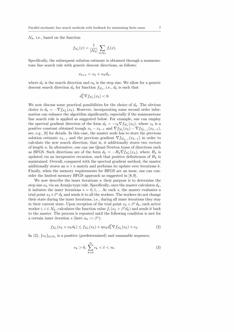
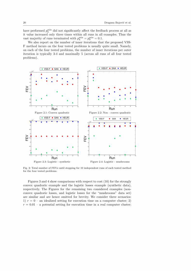
The results on the analysis of FEVs are shown at Figure 2. The (green)diamonds show the costs for each run of VSS-F, the (red) dots are the costs ofSAA while the (blue) squares are the costs of HEUR, for each run, expressedas the number of function evaluations, FEV. The cost reduction obtainedby VSS-F with respect to both competitors is rather significant. For convexquadratic the savings are ranging form 20% to 50%, Figure 2.1. In the caseof non-convex quadratic the savings are even larger, going up to 80%, Figure2.2. The same is happening with the synthetic logistic loss example - we havethe reduction of up to 50%, Figure 2.3. In 2 runs considering the real dataset, non of the tested schemes converged within 107 FEVs. For the remainingruns, the savings are from 25% to 70% regarding SAA and similar results holdfor HEUR.

It is important to comment here the role of safeguard parameters in the ac-tual implementation of the algorithm. As already explained pmin

k is importantfrom the theoretical point of view as this sequences ensures that the full setof nodes is employed eventually. Thus it might seem that pmin

k actually inter-feres with the feedback mechanism and thus might even reduce the relativelycomplex mechanism of pk update into mere increase by a certain schedule.Apparently, that does not happen in actual implementation. In all tests we


have performed pmink did not significantly affect the feedback process at all as

it value increased only three times within all runs in all examples. Thus thevast majority of runs terminated with pmin

k = pmin0 = 0.1.

We also report on the number of inner iterations that the proposed VSS-F method incurs on the four tested problems is usually quite small. Namely,on each of the four tested problems, the number of inner iterations per outeriteration is typically 3-4 and maximally 5 (across all runs of all four testedproblems).

1 2 3 4 5 6 7 8 9 100.7

0.8

0.9

1

1.1

1.2

1.3

1.4

1.5

1.6

1.7x 10

5

Run

FE

V

VSS-F SAA HEUR

1 2 3 4 5 6 7 8 9 100

1

2

3

4

5

6

7x 10

5

Run

FE

V

VSS-F SAA HEUR

Figure 2.1: Convex quadratic Figure 2.2: Non - convex quadratic

1 2 3 4 5 6 7 8 9 102.5

3

3.5

4

4.5

5

5.5

6

6.5x 10

4

Run

FE

V

VSS-F SAA HEUR

1 2 3 4 5 6 7 8 9 103

4

5

6

7

8

9

10

11x 10

6

Run

FE

V

VSS-F SAA HEUR

Figure 2.3: Logistic - synthetic Figure 2.4: Logistic - mushrooms

Fig. 2: Total number of FEVs until stopping for 10 independent runs of each tested methodfor the four tested problems.

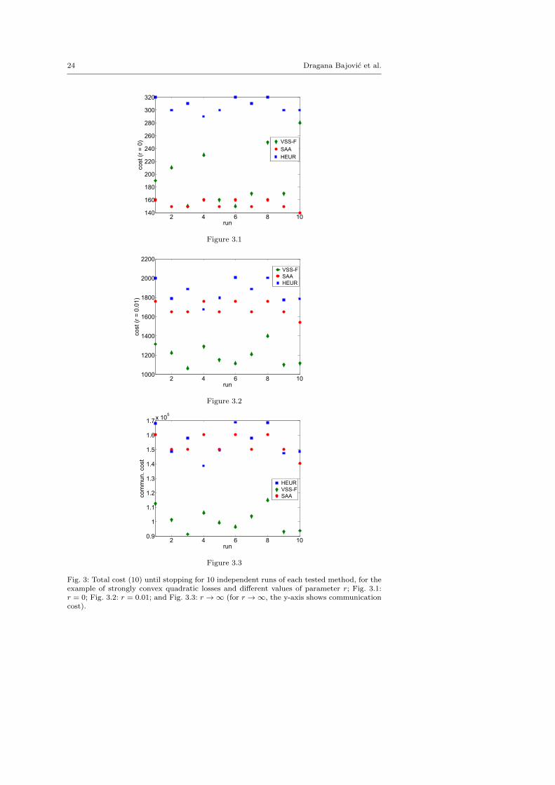
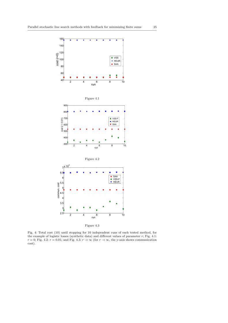
Figures 3 and 4 show comparisons with respect to cost (10) for the stronglyconvex quadratic example and the logistic losses example (synthetic data),respectively. The Figures for the remaining two considered examples (non-convex quadratic losses, and logistic losses for the “mushrooms” data set)are similar and are hence omitted for brevity. We consider three scenarios:1) r = 0 – an idealized setting for execution time on a computer cluster; 2)r = 0.01 – a potential setting for execution time in a real computer cluster;


and 3) r →∞ – an idealized setting for a wireless sensor network. The figurespresent the overall costs (counting both the costs of inner and outer iterations)until stopping for the three values of r (Figures 3.1 and 4.1: r = 0; Figures 3.2and 4.2: r = 0.01; Figures 3.3 and 4.3: r → ∞3) The stopping criterion andthe stopping parameters are the same as in the FEVs comparisons above.

We now comment on the obtained results. Consider first Figure 3.1. Here,as the communication cost (time) is neglected and as the time per inner or perouter iteration does not depend on the number of active workers, it is naturalthat SAA performs the best, as it performs the “most exact” updates amongthe three tested methods. However, when the communication cost is no morenegligible (Figures 3.2 and 3.3), the proposed VSS-F performs better thanboth SAA and HEUR. Similar conclusions can be drawn from the logisticslosses example as well (Figure 4.)

5 Conclusion

We considered a generic nonmonotone line search framework for the minimiza-tion of a finite sum of generic component costs. We assumed a master-workermodel, where the master maintains the solution estimate xk and broadcasts itto the workers. Each worker holds a component cost, and, at each iteration k,it can be in one of the two possible states – active or inactive. At each itera-tion k, active workers evaluate their component costs and the correspondinggradients at the current iterate xk and send this information back to the mas-ter, while inactive workers stay idle. We proposed a mechanism in which themaster node controls the average number of active workers through a singlescalar parameter pk. The master adaptively increases or decreases pk over iter-ations, as needed, based on an inexpensive estimate of the algorithm progress.Hence, the master sends through pk the feedback information to the work-ers as to how many of them should be active at the next iteration to ensureprogress, on the one hand, and save computational cost as much as possible,on the other hand. Simulations on convex and non-convex quadratic lossesand on (convex) logistic losses – both on synthetic and real world data sets– demonstrate the benefits of introducing feedback in the sample size choicealong iterations.

There are several interesting future research directions. First, the frame-work can be specialized and analyzed to more restricted classes of costs. Sec-ond, it is certainly relevant to incorporate in the master-worker model theeffects of several imperfections, like delays and network topology. For exam-ple, if the (master and worker) nodes are organized in a network (e.g., a twodimensional grid), then the gradient and function information from certainworkers will be received with delays, depending on how distant (in terms ofthe number of hops) a worker is from the master; see, e.g., [1]. In this paper,we considered the idealized model, as it represents a necessary starting point

3 For the case r → ∞, computational cost becomes negligible; hence, we plot on the y-axisonly the communication cost, for convenience.


for the analysis of the feedback mechanisms in the control of the sample size.Studying effects of various imperfections like delays represents an interestingfuture research direction.

References

1. A. Agarwal, J. Duchi, Distributed Delayed Stochastic Optimization, proc. Advancesin Neural Information Processing Systems, (2011).

2. F. Bastin, Trust-Region Algorithms for Nonlinear Stochastic Programming and MixedLogit Models, PhD thesis, University of Namur, Belgium, 2004.

3. F. Bastin, C. Cirillo, P. L. Toint, An adaptive Monte Carlo algorithm for com-puting mixed logit estimators, Computational Management Science 3(1), (2006), pp.55-79.

4. F. Bastin, C. Cirillo, P. L. Toint, Convergence theory for nonconvex stochasticprogramming with an application to mixed logit, Math. Program., Ser. B 108, (2006),pp. 207-234.

5. D. P. Bertsekas, Incremental Gradient, Subgradient, and Proximal Methods for Con-vex Optimization: A Survey, Report LIDS – 2848, (2010), pp. 85-119.

6. E. G. Birgin, J. M. Martınez, M. Raydan, Nonmonotone Spectral Projected Gra-dient Methods on Convex Sets SIAM J. Optim. 10(4), (2006), pp. 1196-1211.

7. S. Boyd, N. Parikh, E. Chu, B. Peleato, J. Eckstein, Distributed Optimization andStatistical Learning via the Alternating Direction Method of Multipliers, Foundationsand Trends in Machine Learning, 3(1), (2011), pp. 1-122.

8. R. H. Byrd, G. M. Chin, W. Neveitt, J. Nocedal, On the Use of Stochastic HessianInformation in Optimization Methods for Machine Learning, SIAM J. Optim., 21(3),(2011), pp. 977-995.

9. R. H. Byrd, G. M. Chin, J. Nocedal, Y. Wu, Sample size selection in optimizationmethods for machine learning, Mathematical Programming, 134(1), (2012), pp. 127-155.

10. S.-C. T. Choi, C. C. Paige, M. A. Saunders, MINRES-QLP: A Krylov SubspaceMethod for Indefinite or Singular Symmetric Systems (2011), SIAM Journal on Scien-tific Computing, 33 (4), pp. 1810-1836Read More: http://epubs.siam.org/doi/abs/10.1137/0720052

11. M.A. Diniz-Ehrhardt, J. M. Martınez, M. Raydan, A derivative-free nonmonotoneline-search technique for unconstrained optimization, Journal of Computational andApplied Mathematics, 219(2), (2008), pp. 383-397.

12. R. Fletcher, Conjugate Gradient Methods for Indefinite Systems (1976), in Watson,G. (ed.), Numerical Analysis, LNM, vol. 506, pp. 73-89, Springer, Heidelberg, DOI:10.1007/bfb0080116

13. M. P. Friedlander, M. Schmidt, Hybrid deterministic-stochastic methods for datafitting, SIAM J. Scientific Computing, 34(3), (2012), pp. 1380-1405.

14. D. H. Li, M. Fukushima, A derivative-free line search and global convergence ofBroyden-like method for nonlinear equations, Opt. Methods Software 13, (2000), pp.181-201.

15. Ghadimi, S., Lan, G., Zhang, H, Mini-batch stochastic approximation methodsfor nonconvex stochastic composite optimization, Mathematical Programming, (2016)155: 267. doi:10.1007/s10107-014-0846-1.

16. L. Grippo, F. Lampariello, S. Lucidi, A nononotone line search technique for New-ton’s method, SIAM J. Numerical Analysis, 23(4), (1986), pp. 707-716.

17. F.S. Hashemi, S. Ghosh, R. Pasupathy, On adaptive sampling rules for stochasticrecursion. In S.J. Bickley and J.A. Miller, editors, Proceedings of te 2014 WinterSimulation Conference, Savannah, GA, USA, December 7-10,2014, pages 3959-3970.IEEE/ACM, 2014.

18. N. Krejic, N. Krklec, Line search methods with variable sample size for uncon-strained optimization, Journal of Computational and Applied Mathematics, 245,(2013), pp. 213-231.


19. N. Krejic, N. Krklec Jerinkic, Nonmonotone line search methods with variablesample size, Numerical Algorithms, 68(4), (2015), pp. 711-739.

20. N. Krejic, N. Krklec Jerinkic, Stochastic gradient methods for unconstrained op-timization, Pesquisa Operacional, 34 (3), (2014) 373-39.

21. J. Langford, A. Smola, M. Zinkevich, Slow learners are fast, proc. Advances inNeural Information Processing Systems 22, (2009), pp. 2331-2339.

22. M. Li, D. G. Andersen, J. W. Park, A. J. Smola, A. Ahmed, V. Josifovski,J. Long, E. J. Shekita, B.-Y. Su, Scaling Distributed Machine Learning with theParameter Server (2014).

23. A. Nedic, D. P. Bertsekas, Incremental Subgradient Methods for NondifferentiableOptimization, SIAM J. on Optimization, 12, (2001), pp. 109-138.

24. A. Nedic, A. Olshevsky, Stochastic Gradient-push for Strongly Convex Functions onTime-varying Directed Graphs, available at: http://arxiv.org/abs/1406.2075, (2014).

25. J. Nocedal, S. J. Wright, Numerical Optimization, Springer, 1999.26. R. Pasupathy, On choosing parameters in restrospective-approximation algorithms

for simulation-optimization, proceedings of teh 2006 Winter Simulation Conference,L.F. Perrone, F.P. Wieland, J. Liu, B.G. Lawson, D.M. Nicol and R.M. Fujimoto,eds., pp. 208-215.

27. R. Pasupathy, On Choosing Parameters in Retrospective-Approximation Algorithmsfor Stochastic Root Finding and Simulation Optimization, Operations Research Vol.58, No. 4, pp. 889-901.

28. E. Polak, J. O. Royset, Eficient sample sizes in stochastic nonlinear programing,Journal of Computational and Applied Mathematics, Vol. 217, Issue 2, 2008, pp.301-310.

29. M. Rabbat, R. Nowak, Distributed Optimization in Sensor Networks, Proceedings ofthe 3rd international symposium on Information processing in sensor networks (2004)

30. B. Recht, C. Re, S. J. Wright, F. Niu, Hogwild: A Lock-Free Approach to Paral-lelizing Stochastic Gradient Descent, available at: http://arxiv.org/abs/1106.5730.

31. J. O. Royset, Optimality functions in stochastic programming, Math. Program. Ser.A, DOI 10.1007/s10107-0453-3.

32. Y. Saad, Iterative Solution of Indefinite Symmetric Linear Systems by Methods UsingOrthogonal Polynomials over Two Disjoint Intervals (1983), SIAM J. Numer. Anal.,20(4), pp. 784811

33. M. Schmidt, N. Le Roux, F. Bach, Minimizing Finite Sums with the StochasticAverage Gradient, available at: http://arxiv.org/abs/1309.2388, (2013).

34. O. Shamir, N. Srebro, T. Zhang, Communication Efficient Distributed Optimiza-tion using an Approximate Newton-type Method, 31st International Conference onMachine Learning, ICML (2014).

35. K. I. Tsianos, S. Lawlor, M. G. Rabbat, Communication/ComputationTradeoffs in Consensus-Based Distributed Optimization (2012), available at:https://arxiv.org/abs/1209.1076

36. Uday V. Shanbhag, J.H. Blanchet, budget constrained stochastic optimization. InProceedings of the 2015 Winter Simulation Conference, Huntington Beach, CA, USA,December 6-9, 2015, pages 368-379. IEEE/ACM, 2015.

37. Uday V. Shanbhag, Decomposition and Sampling Methods for Stochastic EquilibriumProblems, PhD thesis, Department of Management Science and Engineering (Opera-tions Research), Stanford University, 2006.

38. F. Yousefian, A. Nedic, U. V. Shanbhag On stochastic gradient and subgradientmethods with adaptive steplength sequences, Automatica 48(1), (2012), pp. 56-67.

39. Y. Zhang, J. C. Duchi, M. Wainwright, Comunication-Efficient Algorithms for Sta-tistical Optimization, Journal of Machine Learning Research, 14(Nov), (2013), pp.3321-3363.

40. H. Zhang, W. W. Hager, A nonmonotone line search technique and its applicationto unconstrained optimization SIAM J. Optim. 4, (2004), pp. 1043-1056.

41. M. Zinkevich, M. Weimer, A. J. Smola, L. Li, Parallelized Stochastic GradientDescent, proc. Advances in Neural Information Processing Systems, (2010).


2 4 6 8 10140

160

180

200

220

240

260

280

300

320

run

cost

(r =

0)

VSS-F

SAA

HEUR

Figure 3.1

2 4 6 8 101000

1200

1400

1600

1800

2000

2200

run

cost

(r =

0.0

1)

VSS-FSAAHEUR

Figure 3.2

2 4 6 8 100.9

1

1.1

1.2

1.3

1.4

1.5

1.6

1.7x 10

5

run

com

mun.

co

st

HEURVSS-FSAA

Figure 3.3

Fig. 3: Total cost (10) until stopping for 10 independent runs of each tested method, for theexample of strongly convex quadratic losses and different values of parameter r; Fig. 3.1:r = 0; Fig. 3.2: r = 0.01; and Fig. 3.3: r → ∞ (for r → ∞, the y-axis shows communicationcost).


2 4 6 8 1040

60

80

100

120

140

160

run

co

st (r

=0)

VSS

HEUR

SAA

Figure 4.1

2 4 6 8 10300

400

500

600

700

800

900

run

cost

(r =

0.0

1)

VSS-F

HEUR

SAA

Figure 4.2

2 4 6 8 102.5

3

3.5

4

4.5

5

5.5

6

6.5

7x 10

4

run

com

mun.

co

st

SAAVSS-FHEUR

Figure 4.3

Fig. 4: Total cost (10) until stopping for 10 independent runs of each tested method, forthe example of logistic losses (synthetic data) and different values of parameter r; Fig. 4.1:r = 0; Fig. 4.2: r = 0.01; and Fig. 4.3: r → ∞ (for r → ∞, the y-axis shows communicationcost).

Documents

Parallel stochastic line search methods with feedback for ...people.dmi.uns.ac.rs/~natasa/mainPkminMarch19.pdf · Noname manuscript No. (will be inserted by the editor) Parallel stochastic