Analysis of star camera errors in GRACE data and their

J Geod (2015) 89:551–571DOI 10.1007/s00190-015-0797-1

ORIGINAL ARTICLE

Analysis of star camera errors in GRACE data and their impacton monthly gravity field models

Pedro Inácio · Pavel Ditmar · Roland Klees ·Hassan Hashemi Farahani

Received: 18 March 2014 / Accepted: 19 February 2015 / Published online: 3 March 2015© The Author(s) 2015. This article is published with open access at Springerlink.com

Abstract Star cameras (SCs) on board the GRACE satel-lites provide information about the attitudes of the space-crafts. This information is needed to reduce the K-band rang-ing data to the centre ofmass of the satellites. In this paper,weanalyse GRACE SC errors using two months of real data ofthe primary and secondary SCs.We show that the errors con-sist of a harmonic component,which is highly correlatedwiththe satellite’s true anomaly, and a stochastic component. Webuilt models of both error components, and use these modelsfor error propagation studies. Firstly, we analyse the propa-gation of SC errors into inter-satellite accelerations. A spec-tral analysis reveals that the stochastic component exceedsthe harmonic component, except in the 3–10 mHz frequencyband. In this band, which contains most of the geophysi-cally relevant signal, the harmonic error component is largerthan the random component. Secondly, we propagate SCerrors into optimally filtered monthly mass anomaly mapsand compare them with the total error. We found that SCerrors account for about 18 % of the total error. Moreover,gaps in the SC data series amplify the effect of SC errors bya factor of 5. Finally, an analysis of inter-satellite pointingangles for GRACE data between 2003 and 2010 reveals thatinter-satellite ranging errors were exceptionally large dur-ing the period February 2003 till May 2003. During thesemonths, SC noise is amplified by a factor of 3 and is a con-siderable source of errors in monthly GRACEmass anomalymaps. In the context of future satellite gravity missions, thenoise models developed in this paper may be valuable formission performance studies.

P. Inácio (B) · P. Ditmar · R. Klees · H. H. FarahaniDelft University of Technology,Stevinweg 1, 2624 CN Delft, The Netherlandse-mail: [email protected]

Keywords Star cameras · Future gravitymissions ·K-bandranging · Attitude errors · Antenna phase centre correction

1 Introduction

The Gravity Recovery And Climate Experiment (GRACE)satellites (Tapley et al. 2004) were launched in 2002 with theaim to measure the static and time-variable gravity field ofthe Earth. TheGRACEmission consists of two satellites, fol-lowing each other in a low-earth orbit separated by a distanceof about 200 km. The attitudes of the GRACE satellites aredetermined by two star cameras (SCs) on board each satel-lite. Errors in the SC measurements result in an inaccuratedetermination of the satellites’ attitudes, which ultimatelypropagate into errors in monthly mass anomaly maps.

Simulation studies (Kim 2000) done prior to the launch ofthe GRACE satellites predicted a noise level, which has notyet beenmatched by real data (Schmidt et al. 2008). This dis-crepancy highlights the need to fully understand the overallerror budget. This is a goal on its own butmay also be relevantfor future mission performance analysis depending on theoverallmission concept. In a recent study,Ditmar et al. (2012)explain the major contributions to the GRACE noise budgetin different spectral bands. They show that low-frequencynoise (<1 mHz) is caused by the limited accuracy of thecomputed GRACE orbits, while the K-band ranging (KBR)sensor is the major contributor to noise at frequencies above9 mHz. Noise in the frequency band between 1 to 9 mHz(5.4–49 cycles per revolution, cpr) is less well understood.Although there is no one-to-one correspondence between fre-quencies in the KBR data and spherical harmonic degrees, itis very likely that relevant geophysical signal largely mapsinto this frequency range.

123

http://crossmark.crossref.org/dialog/?doi=10.1007/s00190-015-0797-1&domain=pdf

552 P. Inácio et al.

The fundamental observable of GRACE is the rangebetween the satellites,which ismeasured by theKBRsystem.Since the launch of GRACE, advances in ranging technologyallow theuseof laser interferometers in satellites (Dehne et al.2009). For instance, the GRACE follow-on (GRACE-FO)mission is scheduled to be launched in August 2017 (Sheardet al. 2012). Thismissionwill carry bothKBR and laser inter-ferometric ranging instruments, the latter as a technologicalshowcase. It is foreseen that laser interferometers will beable to improve the ranging accuracy by up to three ordersof magnitude (Dehne et al. 2009; Bender et al. 2003). How-ever, improvements brought by laser interferometry alonedo not guarantee similar improvements in monthly gravityanomaly maps. Fully exploiting the new ranging technol-ogy requires all other relevant error sources to be controlled.Before GRACE’s launch, pre-mission simulation studies hadto rely on assumptions about error sources. At this point, realdata of the GRACE mission can be used to understand thecomplete error budget. This knowledge may be important forthe simulation and design of future GRACE-type missions.

Errors in attitude determination may propagate intoGRACE-based gravity models either by causing errors inthe orientation of the measured non-gravitational accelera-tion vector or by causing ranging errors.

In the context of the gravity field and steady-state oceancirculation explorer (GOCE) mission (Drinkwater et al.2007), errors in satellite attitude are well understood. Pail(2005) documents a simulation study on attitude errors. Heconsiders various scenarios of errors in the attitude prod-uct, and their impact on GOCE gravity gradients is shown.Frommknecht et al. (2011) provide details about the atti-tude reconstruction step of the GOCE data processing. Theyused the so-called hybridization approach to merge informa-tion provided by the gradiometer and the star tracker instru-ments using a Kalman filter. Building on this, Stummer et al.(2012) document improvements to the attitude reconstruc-tion method, where a new FIR filter approach replaces theKalman filter. All these publications rely on a priori knowl-edge of the errors in the SC instruments aboard GOCE. Anexception is Stummer et al. (2011), where an estimate of realerrors in SC instruments is shown.

Regarding the GRACE mission, the impact of errors inthe satellite attitudes has not yet been fully addressed. Inter-satellite accelerations (ISAs) reflecting gravity field varia-tions need to be corrected for non-gravitational accelera-tions. The latter are measured by accelerometers on boardthe GRACE satellites. The measurements refer to the sci-ence reference frame (SRF) (Case et al. 2010), and need tobe rotated to the inertial reference frame (IRF) in which theISAs are expressed. Attitude errors cause small deviations inthe orientation of the non-gravitational acceleration vectorin inertial space, which ultimately show up as errors in theISAs.

Observed inter-satellite ranges refer to the antenna phasecentres, but need to be reduced to the centre of mass (CoM)of each GRACE satellite. The corresponding correction isreferred to as the antenna phase centre correction (APC).This type of correction is applied to both the GPS and KBRmeasurements. The APC is computed as the projection ofthe estimated antenna phase centre vector along the directiondefined by the two CoM of the satellites. This computationrequires the antenna phase centre vector to be rotated fromthe SRF to the IRF. Inaccuracies in the satellite attitudesintroduce errors in reduced GPS and KBR measurements.In this paper, we focus only on the APC errors in the KBRranging data.

The KBR ranging data and the corresponding APC arepublicly available as the KBR1B product, which is part ofthe set of GRACE Level-1B (L1B) products (Case et al.2010). Other relevant products are the KBR antenna phasecentre vector product (VKB1B) and the orientation of eachSC head with respect to the SRF (QSA1B). Horwath et al.(2011) identified biases in the pitch and yaw angles of L1Battitude data, which introduce errors in the APC. Horwathet al. also showed improvements in gravity field solutionswhen removing them. Bandikova et al. (2012) conducted astudy on the inter-satellite pointing angles and found sys-tematic effects with the potential to affect GRACE gravityfield solutions. In 2012, a new release (RL02) of L1B datahas been made available. Following up on the improvementsproposed by Horwath et al., the new RL02 version bene-fits from a recalibration of the QSA1B and VKB1B prod-ucts (Kruizinga et al. 2010). These results strongly supportthe hypothesis that errors in APC of KBR data may playa role in GRACE final products and motivate the need tobetter understand their propagation into gravity field solu-tions.

There are twomain objectives of this study. Thefirst objec-tive is to estimate andmodel actual errors inGRACESCdata.Errors in SC data are obtained by exploiting the existing SCredundancy on board the GRACE satellites. SC data are partof the GRACE Level-1A (L1A) data products (Case et al.2010). Using L1A SC data, we build models that describeerrors along individual axes of GRACE SCs. These mod-els allow us to propagate realistic SC errors into gravity fieldmodels andmay be used to simulate SC errors under differentscenarios.

The second objective is to assess the impact of estimatedattitude errors on GRACE monthly gravity anomaly maps.Realizations of SC attitude errors are first propagated intoKBR errors and then into ISA (Liu et al. 2010). From ISA,monthly mass anomaly maps are estimated using the proce-dure of Liu et al. (2010). The effect of attitude noise on themonthly mass anomaly maps is assessed by comparing themwith monthly mass anomaly maps obtained in the presenceof synthetic SC noise.

123

Analysis of star camera errors in GRACE data 553

The structure of the paper is as follows. In Sect. 2, weprovide background information about SCs and their config-uration in GRACE satellites. In Sect. 3, we analyse real L1ASC data and quantify noise in individual SC axes. The noiserealizations are then used in Sect. 4 to build models of atti-tude noise. In Sect. 5, we discuss the propagation of attitudeerrors into GRACE inter-satellite ranging data. In Sect. 6, weshow the propagation of the SC error models into the satelliteattitudes, ISA and monthly gravity field solutions. In Sect. 7,we provide a brief summary of themain findings of the study.Finally, in Sect. 8, we discuss the results obtained and discusspotential applications to future satellite gravimetry missions.

2 Star cameras

A SC is an instrument comprising a digital camera, a micro-processor, software, and a star catalogue (Liebe 2002). Thestar catalogue contains information about the position of thestars in the celestial sphere. The SC views a small portion ofthe sky and pinpoints the brightest stars in its field of view.The pattern formed by the brightest stars is comparedwith theinternal star catalogue allowing the instrument to recognizethe stars in thefield of view.TheSC instrument uses advancedalgorithms to compute the (sub-)pixel coordinates of the cen-tres of the stars in the field of view. Knowing the location ofthe brightest stars in the camera’s internal reference frame,the attitude of the SC instrument and consecutively that ofthe spacecraft can be determined.

The origin of the SC internal reference frame is the cen-tre of the optical system’s field of view. Its orientation isdefined with a boresight axis (typically the z-axis) crossingthe centre of the field of view and pointing perpendicular toit. The x- and y-axes are coplanar to the field of view and aretypically named cross-boresight axes. The rotation betweenthis reference frame and the SRF is obtained through cali-bration procedures, and is provided as the quaternion productQSA1B (Case et al. 2010).

The distinction between boresight and cross-boresightis motivated by the fact that SCs do not deliver isotropicaccuracy on the rotation about all three axes (Liebe 2002).Typically, SCs are more sensitive to rotations about thecross-boresight axes than about the boresight axis. Rotationsaround the cross-boresight axes are seen by the optical sys-tem as a translation of all the stars in the field of view. Thedisplacement of the star centroids is uniform across thewholeimage. On the other hand, rotations around the boresight axisresult in rotations of the stars around the centre of the field ofview. Stars close to the centre show much smaller displace-ments than those at the edge. As a result, the ratio betweenthe accuracy of the cross-boresight and the boresight axes oftypical SCs is somewhere between 6 and 20 (Liebe 2002).For GRACE SCs, the accuracy of rotations about the cross-

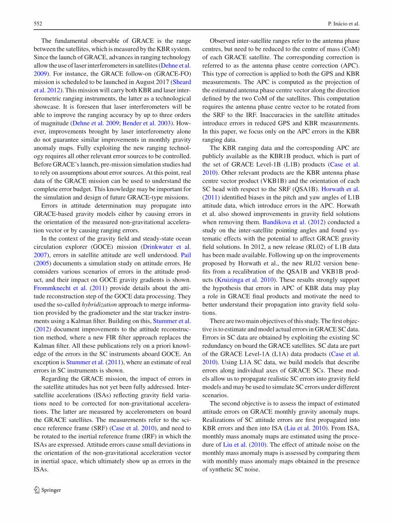
Fig. 1 Primary SC (P), secondary SC (S) and science (C) referenceframes. Blue represents x-, green represents y- and red is the boresightaxis represented by the letter z. Both SCs are assembled at ±135◦ rota-tion angle about the x-axis in the science reference frame (SRF)

boresight axes is better than that of rotations about the bore-sight axis by a factor of 8 (Wu et al. 2006, [Appendix J]).

It is common practice that satellites use two (ormore) SCs,looking at different parts of the sky. This has two advantages;first of all, combining data of several SCs improves the accu-racy of attitude information, in particular if the configurationhas been properly designed to reduce the anisotropic sen-sitivity of each camera. Secondly, several cameras provideredundancy; should one of the sensors fail or look towardsthe Sun or the Moon, the others are still available to provideattitude information.

The GRACE satellites are equipped with two SCs each,which provide attitude information with 1 s sampling. Theyare referred to as primary and secondary SC, respectively.Figure 1 depicts the relative orientation between each of theSC’s reference frame and the SRF.

3 Attitude errors

In this section, we provide the basic formalism of rotationsand showhowwe exploit the data of the two independent SCsto quantify attitude errors. The presence of two SCs on boardeach GRACE satellite provides redundant measurements ofthe satellites’ attitude. The difference between the SC mea-surements reflects the level of noise in the instruments. Wewill define the SC measurement errors as small-angle rota-tions. Then we show how noise in individual SC data prop-agates into the difference between primary and secondarySCs. This formalism allows us to estimate errors along indi-vidual SC axes based on the observed differences betweenSC measurements.

The relative orientation of two arbitrary reference framescan be modelled in different ways, using either directioncosine matrices (DCMs), quaternions or angle-axis vectors.In Aerospace Engineering, it is frequently needed to definerotations between the reference frame of a vehicle and someexternal reference frame. The most intuitive way to describe

123


the rotation is to use Cardan angles: roll (α), describing therotation around the x-axis, which in this paper is the along-track direction; yaw (γ ) around the z-axis which is normallyperpendicular (either up or down) to the horizontal plane ofthe vehicle, and pitch (β) around the y-axis, which is cho-sen to complete the right-handed system. These angles aremost commonly used since they correspond to the types ofrotations used to manoeuvre aircraft and spacecraft. This setof three rotations can be used to define the orientation of thespacecraft relative to some reference frame.

Each SC on board the GRACE satellites provides attitudeinformation relative to the IRF. In the following, superscriptC refers to the science reference frame (SRF), common to allstar cameras, Si to the i-th star camera reference frame, andI to the IRF. To the unacquainted reader, a short introduc-tion to rotations is provided in Appendix A. Several specificreferences on the topic can be found, e.g. Jekeli (2001).

Let RSiI be the DCM, which transforms vectors from the

IRF to the i-th SC frame. Each SC measures this rotationwith a small error εψ,i .

RSiI = R(εψ,i )R

SiI , (1)

where εψ,i ≡ [εα,i εβ,i εγ,i

]Tis the vector representing the

errors in the roll (εα,i ), pitch (εβ,i ) and yaw (εγ,i ) angles in themeasured rotation and where i can be P or S denoting theprimary or secondary star camera, respectively. R(εψ,i ) isthe direction cosine matrix defined by the vector εψ,i , cf.,Appendix A. The tilde denotes a measured quantity. Thesmall-angle errors εψ,i in the SC frame are assumed to bestationary and well described by a Gaussian distribution.

The relative orientation of each SCwith respect to the SRFis known (QSA1B product) and the I → C rotation can bewritten as

RCI,i = RC

SiR(εψ,i )RSiI . (2)

Both SCsmeasure the same rotationRCI and their differences

expose the level of noise in the attitude determination system.Equation (2) allows us to describe the differential rotation asa function of the errors εψ,i and εψ, j in the i-th and j-th SCs.The differential rotation between measurements of any twoSCs is

RCI,i

(RC

I, j

)−1 = RCSi R(εψ,i )R

SiI

(RC

Sj R(εψ, j )RS jI

)−1

= RCSi R(εψ,i )R

SiI R I

S j R(−εψ, j )RS jC (3)

Notice that RbcR

ca = Rb

a = RbdR

da . Therefore,

RCI,i

(RC

I, j

)−1 = RCSi R(εψ,i )R

SiC RC

Sj R(−εψ, j )RS jC

For small errors εψ , the approximationR(εψ) ≈ I−� holds(cf. Appendix A),

= RCSi

(I − �

Sii

)RSiC RC

Sj

(I + �

S jj

)R

S jC

= I − RCSi �

Sii RSi

C + RCSj �

S jj R

S jC − RC

Si �Sii RSi

C RCSj �

S jj R

S jC

(4)

Neglecting second order terms, we obtain from Eq. (31),

RCI,i

(RC

I, j

)−1 ≈ I − �Ci + �C

j

= I − ��Ci j

= R(�εCψ,i j ) (5)

where,

�εCψ,i j ≡ εCψ,i − εCψ, j .

For each GRACE satellite, equipped with primary and sec-ondary SCs, the differential rotation between individual SCmeasurements can be computed as

RCI,P

(RC

I,S

)−1 ≈ R(�εCψ). (6)

In Eq. (6), the rotation I → C as measured by the primarySC is applied after the inverse rotation as measured by thesecondary SC. If both SC measurements are error free, thisoperation would result in the identity matrix. In reality, thisoperation yields a small-angle rotation R(�εCψ), which iscaused by the measurement errors in the SCs. Equation (6)shows that the measurement error �εCψ , in terms of roll,pitch and yaw angles, can be computed directly from theSC data.

Because of the anisotropy of the SC instruments it isimportant to understand how errors in each SC axis propagateinto �εCψ , specifically in terms of their cross- and boresight

axes. Equation (5) shows that attitude errors �εCψ in the C-frame equal the difference between errors in the individualSCs rotated to the C-frame. Using the approximate rotationmatrix from each SC frame to the SRF (see Fig. 1), we readilyobtain

�εCψ = Rx (−135◦)εψ,P − Rx (135◦)εψ,S . (7)

Notice that Eq. (7) is only valid when assuming that SCerrors are small, i.e. in the range where sin θ can beapproximated by θ and cos θ by 1. The following equal-ities hold: cos(±135◦) = − 1√

2, sin(±135◦) = ± 1√

2,

and Eq. (7) can be expanded into component-wise nota-tion:

123


⎡

⎢⎢⎣

�εα

�εβ

�εγ

⎤

⎥⎥⎦ =

⎡

⎢⎢⎣

εα,P − εα,S

1√2

(−εβ,P + εγ,P + εβ,S + εγ,S)

1√2

(−εβ,P − εγ,P − εβ,S + εγ,S)

⎤

⎥⎥⎦ . (8)

The right-hand side can be simplified by adding and subtract-ing the pitch and yaw errors,

⎡

⎢⎢⎣

�εα

�εβ − �εγ

�εβ + �εγ

⎤

⎥⎥⎦ =

⎡

⎢⎢⎣

εα,P − εα,S

2√2

(εγ,P + εβ,S

)

2√2

(−εβ,P + εγ,S)

⎤

⎥⎥⎦ . (9)

Notice that the errors εα,i , εβ,i correspond to the cross-boresight axes, while εγ,i corresponds to the boresight axisof a SC. Boresight errors are expected to be a factor 8 largerthan cross-boresight errors. Based on Eq. (9), we deriveexpressions for the attitude errors of each SC, where weneglect the cross-boresight terms in the second and thirdlines:

⎡

⎢⎢⎣

εα,P − εα,S

εγ,P

εγ,S

⎤

⎥⎥⎦ =

⎡

⎢⎢⎢⎣

�εα

√22

(�εβ − �εγ

)

√22

(�εβ + �εγ

)

⎤

⎥⎥⎥⎦

. (10)

Under the assumption of independent and identically dis-tributed errors in primary and secondary SC data, Eq. (10)allows us to relate differences between SC measurementswith errors along the boresight axis of each SC (εγ,P andεγ,S) and along a combination of one cross-boresight axis(the x-axes) of each SC. It can also be seen that the cross-boresight axes errors εβ,i (the y-axes) are not estimated. Inthe following, we refer to the left-hand side as SC error andto the right-hand side as SC error estimates.

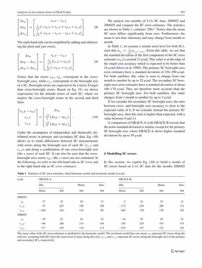
We analyse two months of L1A SC data: 2006/02 and2006/05 and compute the SC error estimates. The statisticsare shown in Table 1, columns “Obs”. Notice that the meanSC error differs significantly from zero. Furthermore, themean is not time stationary and may change from month tomonth.

In Table 1, we assume a similar error level for both SCs,such that σεα = 1√

2σεα,P−εα,S . From this table, we see that

the standard deviation of the first component of the SC errorestimates (εα) is around 23 µrad. This value is at the edge ofthe single axis accuracy which is expected to be better than24 µrad (Davis et al. 1999). The primary SC boresight axeserror estimates have a standard deviation of 230–290 µrad.For both satellites, this value is seen to change from onemonth to another by up to 25 µrad. The secondary SC bore-sight axes error estimates have a standard deviation of about160–170 µrad. They are therefore more accurate than theprimary SC boresight axes. For both satellites, this valuechanges from 1 month to another by up to 3 µrad.

If we consider the secondary SC boresight axes, the ratiobetween cross- and boresight axes accuracy is close to theexpected value of 8. If we consider instead the primary SCboresight axes, then this ratio is higher than expected, with avalue between 9 and 13.

A comparison of GRACE-A with GRACE-B reveals thatthe noise standard deviation is similar, except for the primarySC boresight axis, where GRACE-A shows higher standarddeviations by up to 59 µrad.

4 Modelling SC errors

In this section, we exploit Eq. (10) to build a model ofSC errors based on L1A SC data for the months 2006/02

Table 1 Statistics of SC error estimates, fitted harmonic model and stochastic model in µrad

µrad GRACE-A GRACE-B

Obs. Harm. Stoc. Obs. Harm. Stoc.

Mean Std Std Std Mean Std Std Std

2006/02

εα 27 23 18 13 2 24 19 14

εγ,P 97 263 198 158 −172 254 209 131

εγ,S −168 162 124 98 264 170 130 103

2006/05

εα −10 22 16 14 −16 25 18 16

εγ,P −66 288 214 164 245 229 163 143

εγ,S 117 165 110 113 −234 167 122 101

The mean value of the SC error estimates is attributed to the harmonic model. The stochastic model has zero mean. εα represent SC errors along theroll axis, assuming both SCs have the same level of noise along this axis. εγ,P and εγ,P represent SC errors along the boresight axis of the primaryand secondary SCs, respectively

123


and 2006/05. It can be used to cover the existing datagaps. It can also be used to study the impact of SCerrors on gravity field solutions, in months during whichwe have no SC data. Such model could also be usedto investigate alternative configurations of the SC assem-bly.

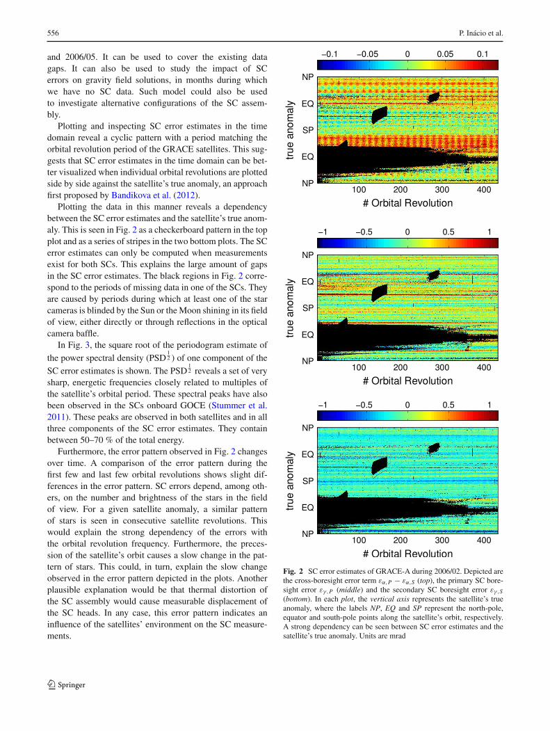
Plotting and inspecting SC error estimates in the timedomain reveal a cyclic pattern with a period matching theorbital revolution period of the GRACE satellites. This sug-gests that SC error estimates in the time domain can be bet-ter visualized when individual orbital revolutions are plottedside by side against the satellite’s true anomaly, an approachfirst proposed by Bandikova et al. (2012).

Plotting the data in this manner reveals a dependencybetween the SC error estimates and the satellite’s true anom-aly. This is seen in Fig. 2 as a checkerboard pattern in the topplot and as a series of stripes in the two bottom plots. The SCerror estimates can only be computed when measurementsexist for both SCs. This explains the large amount of gapsin the SC error estimates. The black regions in Fig. 2 corre-spond to the periods of missing data in one of the SCs. Theyare caused by periods during which at least one of the starcameras is blinded by the Sun or theMoon shining in its fieldof view, either directly or through reflections in the opticalcamera baffle.

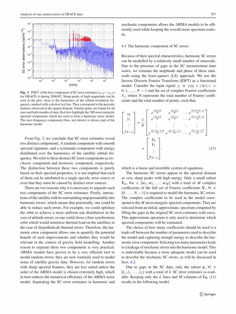
In Fig. 3, the square root of the periodogram estimate of

the power spectral density (PSD12 ) of one component of the

SC error estimates is shown. The PSD12 reveals a set of very

sharp, energetic frequencies closely related to multiples ofthe satellite’s orbital period. These spectral peaks have alsobeen observed in the SCs onboard GOCE (Stummer et al.2011). These peaks are observed in both satellites and in allthree components of the SC error estimates. They containbetween 50–70 % of the total energy.

Furthermore, the error pattern observed in Fig. 2 changesover time. A comparison of the error pattern during thefirst few and last few orbital revolutions shows slight dif-ferences in the error pattern. SC errors depend, among oth-ers, on the number and brightness of the stars in the fieldof view. For a given satellite anomaly, a similar patternof stars is seen in consecutive satellite revolutions. Thiswould explain the strong dependency of the errors withthe orbital revolution frequency. Furthermore, the preces-sion of the satellite’s orbit causes a slow change in the pat-tern of stars. This could, in turn, explain the slow changeobserved in the error pattern depicted in the plots. Anotherplausible explanation would be that thermal distortion ofthe SC assembly would cause measurable displacement ofthe SC heads. In any case, this error pattern indicates aninfluence of the satellites’ environment on the SC measure-ments.

Fig. 2 SC error estimates of GRACE-A during 2006/02. Depicted arethe cross-boresight error term εα,P − εα,S (top), the primary SC bore-sight error εγ,P (middle) and the secondary SC boresight error εγ,S(bottom). In each plot, the vertical axis represents the satellite’s trueanomaly, where the labels NP, EQ and SP represent the north-pole,equator and south-pole points along the satellite’s orbit, respectively.A strong dependency can be seen between SC error estimates and thesatellite’s true anomaly. Units are mrad

123


Fig. 3 PSD12 of the first component of SC error estimates (εα,P −εα,S)

for GRACE-A during 2006/02. Sharp peaks of high magnitude can beseen in the plot, close to the harmonics of the orbital revolution fre-quency, marked with a dashed red line. They correspond to the periodicfeatures observed in the spatial domain. Similar peaks are found for allaxes and both months of data. Red dots highlight the 300 most energeticspectral components which are used to form a harmonic noise model.The zero-frequency component (bias, not shown) is always part of theharmonic model

From Fig. 3, we conclude that SC error estimates revealtwo distinct components. A random component with smoothspectral signature, and a systematic component with energydistributed over the harmonics of the satellite orbital fre-quency.We refer to these distinct SC error components as sto-chastic component and harmonic component, respectively.The distinction between these two components is purelybased on their spectral properties; it is not implied that eachof them can be attributed to a single specific error source oreven that they must be caused by distinct error sources.

There are two reasons why it is necessary to separate suchtwo components of the SC error estimates. Firstly, interac-tions of the satellitewith its surroundingmappresumably intoharmonic errors, which means that potentially, one could beable to reduce such errors. For example, we could optimizethe orbit to achieve a more uniform star distribution in thecase of attitude errors; or one could chose a Sun-synchronousorbit which would minimize thermal load on the satellites inthe case of (hypothetical) thermal errors. Therefore, the har-monic error component allows one to quantify the potentialbenefit of such improvements and whether they would berelevant in the context of gravity field modelling. Anotherreason to separate these two components is very practical.ARMA models have proven to be a very efficient tool tomodel random errors; they are now routinely used to modelnoise of satellite gravity data. However, for random errorswith sharp spectral features, they are less suited unless theorder of the ARMA model is chosen extremely high, whichin turn reduces the numerical efficiency of the ARMA noisemodel. Separating the SC error estimates in harmonic and

stochastic components allows the ARMA models to be effi-ciently used while keeping the overall noise spectrum realis-tic.

4.1 The harmonic component of SC errors

Because of their spectral characteristics, harmonic SC errorscan be modelled by a relatively small number of sinusoids.Due to the presence of gaps in the SC measurement timeseries, we estimate the amplitude and phase of these sinu-soids using the least-squares (LS) approach. We use theInverse Discrete Fourier Transform (IDFT) as a functionalmodel. Consider the input signal yi ≡ y(t0 + i�t), i =0, 1, . . . , N − 1 and the set of complex Fourier coefficientsY j , where N represents the total number of Fourier coeffi-cients and the total number of points, such that,

⎡

⎢⎢⎢⎣

y0y1...

yN−1

⎤

⎥⎥⎥⎦

= 1

N

⎡

⎢⎢⎢⎢⎢⎣

ei2π ·0·0

N ei2π ·0·1

N · · · e i2π ·0·(N−1)N

ei2π ·1·0

N ei2π ·1·1

N · · · e i2π ·1·(N−1)N

......

. . ....

ei2π ·(N−1)·0

N ei2π ·(N−1)·1

N · · · e i2π ·(N−1)2N

⎤

⎥⎥⎥⎥⎥⎦

×

⎡

⎢⎢⎢⎣

Y0Y1...

YN−1

⎤

⎥⎥⎥⎦

, (11)

which is a linear and invertible system of equations.The harmonic SC errors appear in the spectral domain

as very sharp peaks with high energy. Only a small subsetYm,∀m ∈ [m1,m2, . . . ,mM ] with a total of M complexcoefficients of the full set of Fourier coefficients Yi ,∀i ∈[0, . . . , N − 1] is required to model the harmonic SC errors.The complex coefficients to be used in the model corre-spond to theM most energetic spectral components. They areselected from an initial, approximate, spectrum computed byfilling the gaps in the original SC error estimates with zeros.This approximate spectrum is only used to determine whichspectral components will be estimated.

The choice of how many coefficients should be used is atrade-off between the number of parameters used to describethe model and capturing enough energy to describe the har-monic error component. Selecting toomany parameters leadsto a leakageof stochastic errors into the harmonicmodel. Thisis undesirable because a more adequate model can be usedto describe the stochastic SC errors, as will be discussed inSect. 4.2.

Due to gaps in the SC data, only the subset yl ,∀l ∈[l1, l2, . . . , lL ] with a total of L SC error estimates is avail-able. Keeping only the L lines and M columns of Eq. (11)results in the following model,

123


⎡

⎢⎢⎢⎣

yl1yl2...

ylL

⎤

⎥⎥⎥⎦

=

⎡

⎢⎢⎢⎢⎢⎣

ei2π ·l1·m1

N ei2π ·l1·m2

N · · · e i2π ·l1·mMN

ei2π ·l2 ·m1

N ei2π ·l2 ·m2

N · · · e i2π ·l2 ·mMN

......

. . ....

ei2π ·lL ·m1

N ei2π ·lL ·m2

N · · · e i2π ·lL ·mMN

⎤

⎥⎥⎥⎥⎥⎦

⎡

⎢⎢⎢⎣

Ym1

Ym2...

YmM

⎤

⎥⎥⎥⎦

.

(12)

We assume that all observations are uncorrelated and havethe same unknown standard deviation σy , so that the SCerror estimates variance–covariance matrix is Cy ≡ σ 2

y I.As seen in Fig. 2, gaps cluster in large regions, resulting inunstable linear system of equations, whose solutions showstrong oscillations in the areas void of data. To mitigate thisbehaviour, we apply regularization (Tikhonov and Arsenin1977), in the form of a set of pseudo-observations, which aredefined only over the gapped regions of the SC error esti-mates. Hence, the extended mathematical model is

[y0

]=

[AAg

]Ym. (13)

The variance–covariance matrix of the pseudo-observationsis Cg ≡ σ 2

g I, where σg is the standard deviation of the noisein the pseudo-observations. Then, the regularized solution isobtained as,

Ym =(ATA + kAT

gAg

)−1 (AT y

), (14)

where k = σ 2y

σ 2gis the regularization parameter. If the standard

deviation of noise in the pseudo-observations is assumed tobe large (σg → ∞) then k → 0. In this situation, no reg-ularization is applied, resulting in potentially unstable LSsolutions. On the other hand, if σg = σy , then k = 1, and,in this case, the pseudo-observations have the same weightas the observations. This is equivalent to assigning zero val-ues to missing data, which, as we argued before, is undesir-able. Thus, both extremes cases, k = 0 and k = 1, lead tosub-optimal results. A certain intermediate value of k corre-sponds to a solution which suitably represents the harmonicSC errors. This solution is defined as the onewhich conservesthe total energy of the harmonic component in the SC errorestimates.

The total energy ξ ′ of the observed harmonic component,which contains data gaps, can be computed as

ξ ′ =∑

m

‖ Ym ‖2 . (15)

However, the fitted harmonicmodel contains no gaps. In viewof Parseval’s identity, the total energy of the observed andfitted harmonic components can only be compared if theobserved harmonic component is up-scaled by the ratio N

L

between the total number and the number of valid SC errorestimates. This means that Eq. (15) must be replaced by theexpression for the up-scaled energy,

ξ = N

L

∑

m

‖ Ym ‖2 (16)

The following procedure is used to fit a harmonic model tothe gapped SC error estimates:

1. Assign zero values to the missing SC error estimates tocompute an approximate PSD. This PSD is used to findthe set of M most energetic frequency components inthe SC error estimates. For one month of data, the PSDyields around 106 Fourier coefficients. However, only100–300 most energetic components typically containbetween 50–70 % of the total energy. In our models, wechose the value of M = 300. This number is empiricallychosen as a threshold beyond which adding more fre-quency components no longer significantly changes thetotal energy of the harmonic component. In Fig. 3, theyare marked with red circles.

2. Compute the target total energy ξ of the harmonic modelfrom the selected set of coefficients Ym, cf., Eq. (16).

3. An initial value of the regularization parameter is chosenand the regularized solution is computed.

4. The regularization procedure is iterated with differentparameters ki , until the obtained solution is within athreshold δ of the target total energy,

∣∣∣∣∣ξ −

∑

m

‖ Ym ‖2∣∣∣∣∣< δ, (17)

If the total energy is too high, the solution needs moreregularization (ki > ki−1). Otherwise the regularizationparameter should be reduced (ki < ki−1).

This procedure yields amodel for the harmonic error com-ponent. In the absence of information in gapped regions,it interpolates the information observed in the regions withmeasurements instead of assuming zero data in the gaps. Wedo not state that such a model represents the real, unknownerrors in the gapped regions. However, we can state that sucha model is the one which, in the whole domain, most closelyrepresents the harmonic error observed in the non-gappedregions.

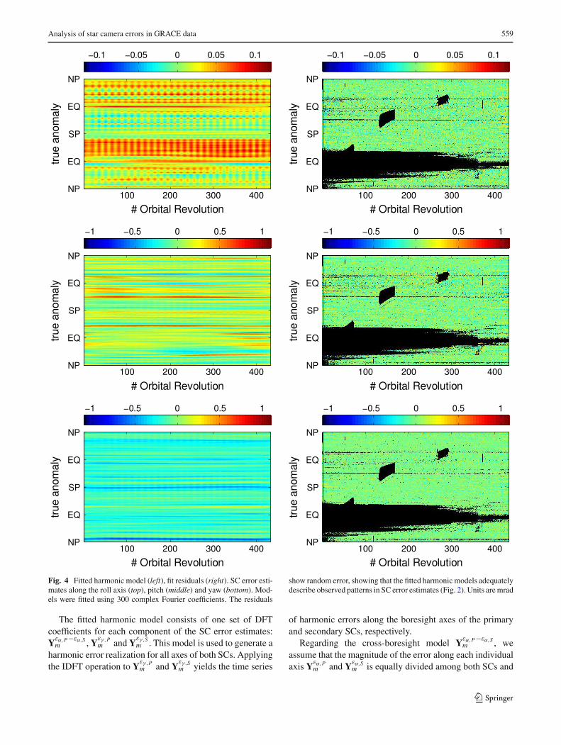
The results of the outlined algorithm are shown in Fig. 4.Table 1 shows the statistics of the fitted harmonic modelsand of the respective residuals. It can be seen that the har-monic model, despite comprising only a small set of fre-quency components, contains ≈65 % of the total SC errorestimates energy.

123


Fig. 4 Fitted harmonic model (left), fit residuals (right). SC error esti-mates along the roll axis (top), pitch (middle) and yaw (bottom). Mod-els were fitted using 300 complex Fourier coefficients. The residuals

show random error, showing that the fitted harmonic models adequatelydescribe observed patterns in SC error estimates (Fig. 2). Units aremrad

The fitted harmonic model consists of one set of DFTcoefficients for each component of the SC error estimates:Yεα,P−εα,Sm , Y

εγ,Pm and Y

εγ,Sm . This model is used to generate a

harmonic error realization for all axes of both SCs. Applyingthe IDFT operation to Y

εγ,Pm and Y

εγ,Sm yields the time series

of harmonic errors along the boresight axes of the primaryand secondary SCs, respectively.

Regarding the cross-boresight model Yεα,P−εα,Sm , we

assume that the magnitude of the error along each individualaxis Yεα,P

m and Yεα,Sm is equally divided among both SCs and

123


that they are orthogonal in the complex plane. This results ina solution,

Yεα,Pm = −

√2

2e−i π

4 Yεα,P−εα,Sm

Yεα,Sm =

√2

2e

π4 Yεα,P−εα,S

m . (18)

These two components are obtained as rotations in the com-plex plane by ±45◦ of the corresponding cross-boresightmodel, scaled to satisfy the observation in Eq. (10). The zero-frequency component (meanvalue) is not an imaginary value.Therefore, assuming that it is also equally divided amongboth SCs, Yεα,P

0 = − 12Y

εα,P−εα,S0 and Yεα,S

0 = 12Y

εα,P−εα,S0

The two remaining cross-boresight axes Yεβ,Pm and Y

εβ,Sm

are not observable, cf., Eq. (10). We assume that the magni-tude of their DFT coefficients is the same asYεα,P

m andYεα,Sm ,

while their phases are randomized.

4.2 The stochastic component of SC errors

The stochastic component of the SC error estimates isobtained by subtracting the harmonic model from the origi-nal SC error estimates. This yields the random measurementerrors shown in the second column of Fig. 4. In this sec-tion, the power spectrum of the stochastic SC error estimatesis computed. An Autoregressive-moving-average (ARMA)model is then fitted to the computed power spectrum (Kleeset al. 2003). Using ARMA models to describe the randomerrors in SC measurements allows generating arbitrary longrealizations with the same spectral signature.

We assume that all cross-boresight stochastic errors, εα,P ,εβ,P , εα,S and εβ,S have the same power spectrum and are

uncorrelated. Then PSD12 (εα,P − εα,S) = √

2 PSD12 (εα),

where PSD12 represents the square root of power spectrum

operator and εα represents the stochastic error along all cross-

boresight axes. Applying the operator PSD12 to Eq. (10)

yields,

⎡

⎢⎢⎢⎣

PSD12 (εα)

PSD12 (εγ,P )

PSD12 (εγ,S)

⎤

⎥⎥⎥⎦

=√2

2

⎡

⎢⎢⎢⎣

PSD12 (�εα)

PSD12(�εβ − �εγ

)

PSD12(�εβ + �εγ

)

⎤

⎥⎥⎥⎦

. (19)

Notice that, similarly to the harmonic component, the pres-ence of gaps in the SC error estimates requires the powerspectrum to be up-scaled by the ratio N

L .Equation 19 yields the power spectra of stochastic errors

along the primary SC boresight axis (εγ,P ), the secondarySC boresight axis (εγ,S) and all the cross-boresight axes ofboth SCs (εα). The ARMA models fitted to each componentof the stochastic SC error are shown in Fig. 5.

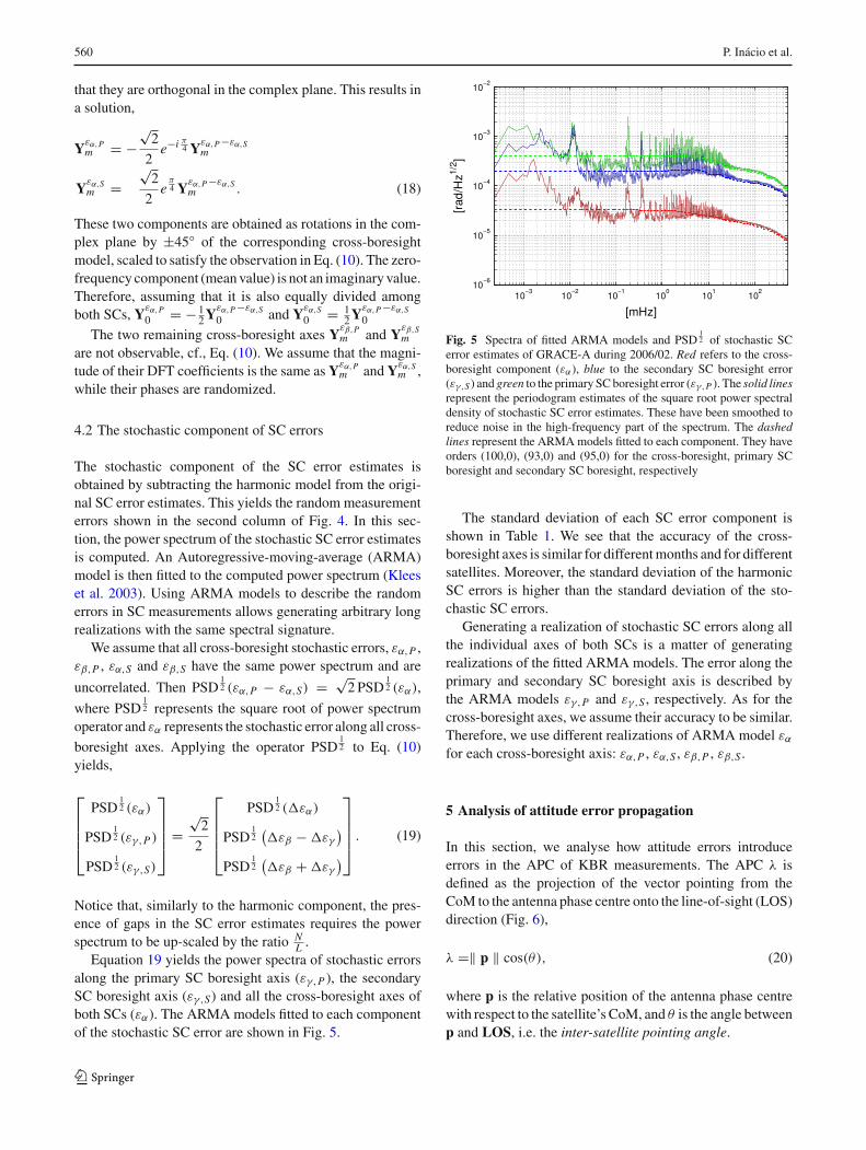
Fig. 5 Spectra of fitted ARMA models and PSD12 of stochastic SC

error estimates of GRACE-A during 2006/02. Red refers to the cross-boresight component (εα), blue to the secondary SC boresight error(εγ,S) and green to the primary SCboresight error (εγ,P ). The solid linesrepresent the periodogram estimates of the square root power spectraldensity of stochastic SC error estimates. These have been smoothed toreduce noise in the high-frequency part of the spectrum. The dashedlines represent the ARMAmodels fitted to each component. They haveorders (100,0), (93,0) and (95,0) for the cross-boresight, primary SCboresight and secondary SC boresight, respectively

The standard deviation of each SC error component isshown in Table 1. We see that the accuracy of the cross-boresight axes is similar for differentmonths and for differentsatellites. Moreover, the standard deviation of the harmonicSC errors is higher than the standard deviation of the sto-chastic SC errors.

Generating a realization of stochastic SC errors along allthe individual axes of both SCs is a matter of generatingrealizations of the fitted ARMA models. The error along theprimary and secondary SC boresight axis is described bythe ARMA models εγ,P and εγ,S , respectively. As for thecross-boresight axes, we assume their accuracy to be similar.Therefore, we use different realizations of ARMA model εα

for each cross-boresight axis: εα,P , εα,S , εβ,P , εβ,S .

5 Analysis of attitude error propagation

In this section, we analyse how attitude errors introduceerrors in the APC of KBR measurements. The APC λ isdefined as the projection of the vector pointing from theCoM to the antenna phase centre onto the line-of-sight (LOS)direction (Fig. 6),

λ =‖ p ‖ cos(θ), (20)

where p is the relative position of the antenna phase centrewith respect to the satellite’s CoM, and θ is the angle betweenp and LOS, i.e. the inter-satellite pointing angle.

123


Fig. 6 Illustration of antenna phase centre correction to KBR data.KBR system measures ρ′, the distance between the antenna phase cen-tres of the two GRACE satellites. The range ρ between the two CoMs isobtained by adding the APC of each satellite to the KBR measurement,ρ = ρ′ + λA + λB . The inter-satellite pointing angles θi represent theangles between vectors pi and the LOS, where i = A, B for GRACE-Aand GRACE-B, respectively

In the presence of attitude errors, the orientation of theantenna phase centre vector pI in the IRF is determinedinaccurately and the inter-satellite pointing angle θ is per-turbed. Let us introduce the noisy quantities θ = θ + εθ andλ = λ+ελ, where we assume that εθ and ελ are normally dis-tributed errors, in the pointing angle and APC, respectively.Linearisation of the APC around the nominal inter-satellitepointing angle yields

σελ =‖ p ‖ sin(θ) σεθ , (21)

where σελ and σεθ is the standard deviation of the errors inthe APC and inter-satellite pointing angles, respectively.

The inter-satellite pointing angle is actively controlled bythe attitude and orbit control system (AOCS).GRACEAOCSis designed to keep these angles below θ < 4 mrad (Hermanet al. 2004). In this range, sin(θ) can be approximated by θ .Furthermore, we assume APC errors of both satellites to beuncorrelated and identically distributed, so that consideringthe contribution of bothGRACE-A andB, yields the standarddeviation

σελ = √2 ‖ p ‖ θ σεθ . (22)

Equation (22) shows that the impact of attitude errorsincreases proportionally to (1) the distance between theantenna phase centre and the CoM and (2) the inter-satellitepointing angle θ .

The distance between the antenna and the CoM is ‖ p ‖≈1.5 m for both satellites. As will be shown in Sect. 6.1, theaccuracy in the determination of the inter-satellite point-ing angle is better than σεθ < 170µrad. Considering aworst-case scenario, according to Eq. (22), the correspond-ing standard deviation of the error in inter-satellite rangesis σελ = 1.4µm. The KBR accuracy is 10µm (Kang et al.2006), whichmeans that the standard deviation of the attitudeerrors is about 7 times smaller than the standard deviation ofthe noise in the KBR ranging data. On the other hand, thestandard deviation alone does not provide a comprehensiveunderstanding of propagated attitude errors. One should also

analyse how the error is distributed over the spectrum. Theremight exist frequency bands at which the impact of attitudeerrors is more substantial than in average.

6 Error propagation

In this section, we analyse towhat extent SC errors contributeto the overall error budget of GRACE time-varying gravityfield models. Section 6.1 describes the propagation of SCerrors into satellite attitude data. The impact of data gaps inthe SC time series is discussed in Sect. 6.2. In Sect. 6.3, thepropagation of attitude errors into inter-satellite accelerationsis discussed. In Sect. 6.4, we discuss the likely impact ofdegraded attitude control. Finally, in Sect. 6.5, we show howSC errors propagate into GRACE gravity field solutions.

6.1 Propagation of SC errors into satellite attitudes

In the presence of multiple SCs, it is necessary to computean estimate of the satellite attitude from all available mea-surements. A description of the official combination methodused by JPL can be found in Romans (2003) and Wu et al.(2006). In Appendix B, this method, originally developed forattitude quaternions, is re-written in terms of direction cosinematrices.

A summary of the official procedure for combining SCmeasurements for GRACE is (Wu et al. 2006):

1. Compute the small-angle difference �εCψ between bothSC measurements, cf., Eq. (6)

2. The optimal correction to the first SC measurement iscomputed, cf., Eq. (39), as

εopt =(�C

1 + �C2

)−1�C

2 �εCψ, (23)

where the information matrix �Ci for each SC in the C-

frame is defined as

�Ci = Rx (±135◦)C−1

i Rx (∓135◦), (24)

and the error variance–covariance matrix Ci for a singleSC is defined as,

Ci =⎡

⎣1 0 00 1 00 0 κ2

⎤

⎦ σ 2, (25)

with σ 2 being the variance of the errors along the SCcross-boresight axes and κ = 8 is the ratio between thestandard deviation of errors along the boresight and thecross-boresight axes (Romans 2003). It can be shown that

123


(�C

1 + �C2

)−1�C

2 = 1

2

⎡

⎣1 0 00 1 −λ

0 −λ 1

⎤

⎦ , (26)

where

λ = κ2 − 1

κ2 + 1.

3. Compute the optimal satellite attitude RCI,opt, cf., (40).

The results of applying this SCmeasurement combinationto synthetic realizations of SC errors for the months 2006/02and 2006/05 are shown in Table 2. The red line in Fig. 7shows the corresponding satellite attitude errors during oneday of 2006/02. From Table 2, we conclude that the pitch andyaw angles of the satellite attitudes are less accurately deter-mined than the roll angles. Errors in the satellites attitudesare therefore not isotropic.

6.2 Quantifying the impact of SC data gaps

There is a relatively large amount of gaps in the SC data (seeTable 2). Gaps reduce the quality of attitude determination.The SC combination procedure described in Sect. 6.1 canonly be applied when both SCs provide data. When one ofthe SCs is inactive, the data from the other SC are used todetermine the attitudes. We quantify the impact of SC datagaps by comparing two error propagation scenarios; in onescenario both SCs are assumed to be constantly active andin the other we use real SC time series to flag time instantswhere one of the SCs is inactive.

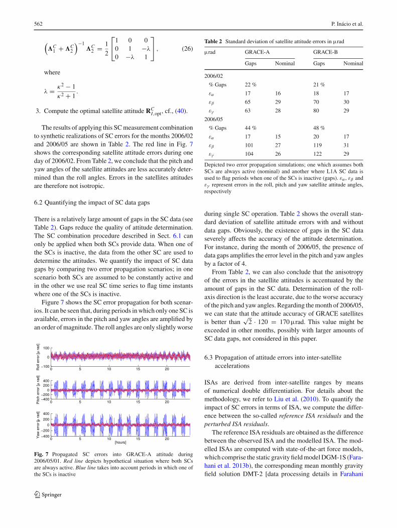
Figure 7 shows the SC error propagation for both scenar-ios. It can be seen that, during periods inwhich only one SC isavailable, errors in the pitch and yaw angles are amplified byan order ofmagnitude. The roll angles are only slightlyworse

Fig. 7 Propagated SC errors into GRACE-A attitude during2006/05/01. Red line depicts hypothetical situation where both SCsare always active. Blue line takes into account periods in which one ofthe SCs is inactive

Table 2 Standard deviation of satellite attitude errors in µrad

µrad GRACE-A GRACE-B

Gaps Nominal Gaps Nominal

2006/02

% Gaps 22 % 21 %

εα 17 16 18 17

εβ 65 29 70 30

εγ 63 28 80 29

2006/05

% Gaps 44 % 48 %

εα 17 15 20 17

εβ 101 27 119 31

εγ 104 26 122 29

Depicted two error propagation simulations; one which assumes bothSCs are always active (nominal) and another where L1A SC data isused to flag periods when one of the SCs is inactive (gaps). εα , εβ andεγ represent errors in the roll, pitch and yaw satellite attitude angles,respectively

during single SC operation. Table 2 shows the overall stan-dard deviation of satellite attitude errors with and withoutdata gaps. Obviously, the existence of gaps in the SC dataseverely affects the accuracy of the attitude determination.For instance, during the month of 2006/05, the presence ofdata gaps amplifies the error level in the pitch and yaw anglesby a factor of 4.

From Table 2, we can also conclude that the anisotropyof the errors in the satellite attitudes is accentuated by theamount of gaps in the SC data. Determination of the roll-axis direction is the least accurate, due to the worse accuracyof the pitch and yaw angles. Regarding themonth of 2006/05,we can state that the attitude accuracy of GRACE satellitesis better than

√2 · 120 = 170µrad. This value might be

exceeded in other months, possibly with larger amounts ofSC data gaps, not considered in this paper.

6.3 Propagation of attitude errors into inter-satelliteaccelerations

ISAs are derived from inter-satellite ranges by meansof numerical double differentiation. For details about themethodology, we refer to Liu et al. (2010). To quantify theimpact of SC errors in terms of ISA, we compute the differ-ence between the so-called reference ISA residuals and theperturbed ISA residuals.

The reference ISA residuals are obtained as the differencebetween the observed ISA and the modelled ISA. The mod-elled ISAs are computed with state-of-the-art force models,which comprise the static gravity fieldmodelDGM-1S (Fara-hani et al. 2013b), the corresponding mean monthly gravityfield solution DMT-2 [data processing details in Farahani

123


(2013)], tidal model EOT11a (Savcenko and Bosch 2012),the model of non-tidal mass redistribution in the atmosphereand oceans AOD1BRL05 (Flechtner et al. 2014), L1B RL02products, and other tidal and relativistic effects. Because themonthly gravity field solution is included in the backgroundforce model, all known signals are removed from the ref-erence ISA residuals. Therefore, we consider the remainingunknown “signal”, i.e. the reference ISA residuals, as an esti-mate of the total error inGRACEdata.Notice that theDMT-2solutions are filtered (or regularized) to prevent propagationof data noise. This is the reason why the reference ISA resid-uals are not zero when the DMT-2 solution is included in thebackground force model.

As compared to DMT-1, a number of improvements areapplied in the production of DMT-2. Firstly, an accuratestochastic description of noise is obtained in the frequencydomain on a monthly basis using ARMA models. Usage ofthese models allows for a proper frequency-dependent dataweighting at the inversion stage. Furthermore, it facilitates anaccurate computation of covariance matrices of noise in esti-mated spherical harmonic coefficients, which are used whenunconstrained monthly solutions are subject to a statisticallyoptimalWiener filter (Klees et al. 2008; Liu et al. 2010). Sec-ondly, data prior to the inversion are subject to an advancedhigh-pass filtering, which uses a spatially dependent weight-ing scheme, so that the low-frequency noise [which is causedby inaccuracies in satellites orbits, Ditmar et al. (2012)] isprimarily estimated based on data collected over areas withminor mass variations, e.g. oceans and deserts. On the onehand, this efficiently suppresses the noise and, on the otherhand, preservesmass transport signals in data. Thirdly, DMT-2 benefits from the usage of the release 2 of GRACE level-1Bdata. Finally, latest background force models are taken intoaccount when the DMT-2 model is produced.

To compute the perturbed ISA residuals, we generate syn-thetic SC errors and propagate them into satellite attitudeerrors. They are added to the measured satellite attitudesresulting in a custom SCA1B satellite attitude product. Fur-thermore, the generated attitudes are used to compute the cor-responding KBR APC, resulting in a custom KBR1B rang-ing product. The perturbed ISA residuals are computed bythe same procedure as the reference ISA residuals, but mak-ing use of the custom SCA1B and KBR1B products. Thedifferences between the two ISAs reflect the impact of thesynthetic SCerrors, and provide an upper boundof the impactof SC errors in terms of ISA and later on in terms of monthlygravity field solutions.

Because both ISAs use realGRACEdata, they contain realSC errors, which are present in the L1B data products. In fact,the perturbed ISA residuals contain SC errors twice; from theGRACE L1B data products and from the synthetic SC errorswe add to the data. However, taking the difference betweenthe reference and perturbed ISA residuals will cancel the

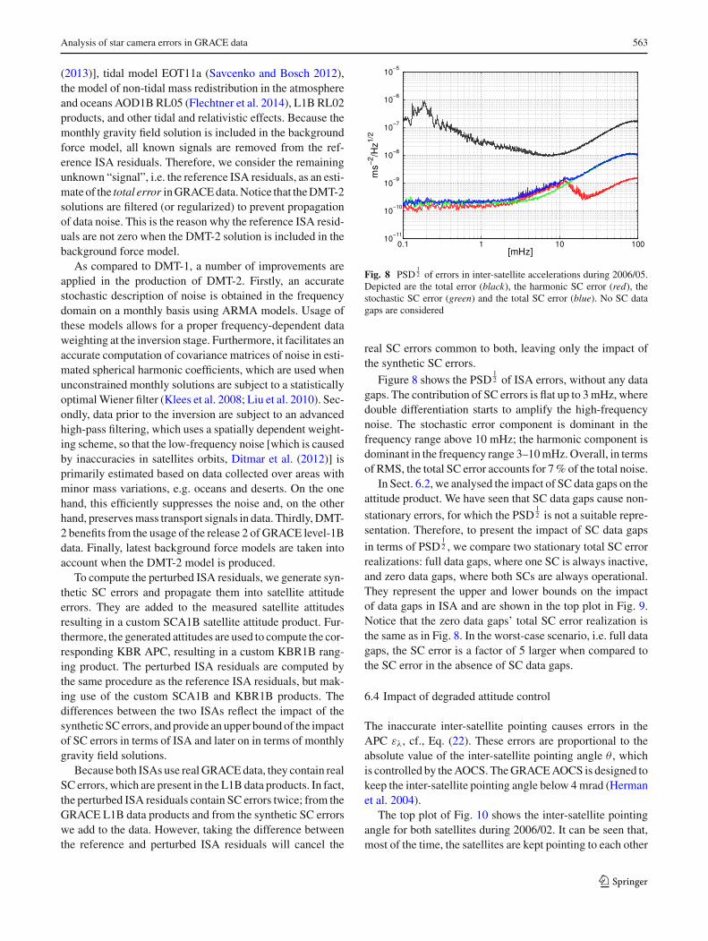
Fig. 8 PSD12 of errors in inter-satellite accelerations during 2006/05.

Depicted are the total error (black), the harmonic SC error (red), thestochastic SC error (green) and the total SC error (blue). No SC datagaps are considered

real SC errors common to both, leaving only the impact ofthe synthetic SC errors.

Figure 8 shows the PSD12 of ISA errors, without any data

gaps. The contribution of SC errors is flat up to 3mHz, wheredouble differentiation starts to amplify the high-frequencynoise. The stochastic error component is dominant in thefrequency range above 10 mHz; the harmonic component isdominant in the frequency range 3–10mHz.Overall, in termsof RMS, the total SC error accounts for 7% of the total noise.

In Sect. 6.2, we analysed the impact of SC data gaps on theattitude product. We have seen that SC data gaps cause non-

stationary errors, for which the PSD12 is not a suitable repre-

sentation. Therefore, to present the impact of SC data gaps

in terms of PSD12 , we compare two stationary total SC error

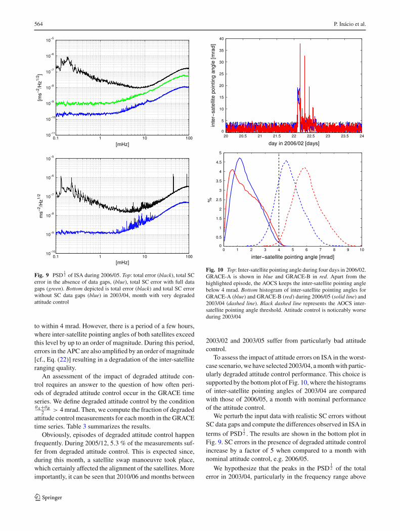
realizations: full data gaps, where one SC is always inactive,and zero data gaps, where both SCs are always operational.They represent the upper and lower bounds on the impactof data gaps in ISA and are shown in the top plot in Fig. 9.Notice that the zero data gaps’ total SC error realization isthe same as in Fig. 8. In the worst-case scenario, i.e. full datagaps, the SC error is a factor of 5 larger when compared tothe SC error in the absence of SC data gaps.

6.4 Impact of degraded attitude control

The inaccurate inter-satellite pointing causes errors in theAPC ελ, cf., Eq. (22). These errors are proportional to theabsolute value of the inter-satellite pointing angle θ , whichis controlled by theAOCS. TheGRACEAOCS is designed tokeep the inter-satellite pointing angle below 4mrad (Hermanet al. 2004).

The top plot of Fig. 10 shows the inter-satellite pointingangle for both satellites during 2006/02. It can be seen that,most of the time, the satellites are kept pointing to each other

123


Fig. 9 PSD12 of ISA during 2006/05. Top: total error (black), total SC

error in the absence of data gaps, (blue), total SC error with full datagaps (green). Bottom depicted is total error (black) and total SC errorwithout SC data gaps (blue) in 2003/04, month with very degradedattitude control

to within 4 mrad. However, there is a period of a few hours,where inter-satellite pointing angles of both satellites exceedthis level by up to an order of magnitude. During this period,errors in the APC are also amplified by an order ofmagnitude[cf., Eq. (22)] resulting in a degradation of the inter-satelliteranging quality.

An assessment of the impact of degraded attitude con-trol requires an answer to the question of how often peri-ods of degraded attitude control occur in the GRACE timeseries. We define degraded attitude control by the conditionθA+θB

2 > 4mrad. Then, we compute the fraction of degradedattitude control measurements for eachmonth in the GRACEtime series. Table 3 summarizes the results.

Obviously, episodes of degraded attitude control happenfrequently. During 2005/12, 5.3 % of the measurements suf-fer from degraded attitude control. This is expected since,during this month, a satellite swap manoeuvre took place,which certainly affected the alignment of the satellites. Moreimportantly, it can be seen that 2010/06 and months between

Fig. 10 Top: Inter-satellite pointing angle during four days in 2006/02.GRACE-A is shown in blue and GRACE-B in red. Apart from thehighlighted episode, the AOCS keeps the inter-satellite pointing anglebelow 4 mrad. Bottom histogram of inter-satellite pointing angles forGRACE-A (blue) and GRACE-B (red) during 2006/05 (solid line) and2003/04 (dashed line). Black dashed line represents the AOCS inter-satellite pointing angle threshold. Attitude control is noticeably worseduring 2003/04

2003/02 and 2003/05 suffer from particularly bad attitudecontrol.

To assess the impact of attitude errors on ISA in the worst-case scenario, we have selected 2003/04, amonthwith partic-ularly degraded attitude control performance. This choice issupported by the bottomplot of Fig. 10, where the histogramsof inter-satellite pointing angles of 2003/04 are comparedwith those of 2006/05, a month with nominal performanceof the attitude control.

We perturb the input data with realistic SC errors withoutSC data gaps and compute the differences observed in ISA in

terms of PSD12 . The results are shown in the bottom plot in

Fig. 9. SC errors in the presence of degraded attitude controlincrease by a factor of 5 when compared to a month withnominal attitude control, e.g. 2006/05.

We hypothesize that the peaks in the PSD12 of the total

error in 2003/04, particularly in the frequency range above

123


Table 3 Fraction of measurements with degraded attitude control within each month in the period 2003–2010 in percentages

January (%) February (%) March (%) April (%) May (%) June (%)

2003 1.81 81.19 87.13 96.67 43.05 0.01

2004 0.11 0.35 0.41 1.38 5.32 0.41

2005 0.20 3.16 0.64 0.06 1.16 0.06

2006 1.16 0.86 0.02 0.07 0.02 0.03

2007 0.01 0.68 0.11 1.01 0.06 1.51

2008 0.25 2.19 0.81 0.62 0.62 0.41

2009 1.19 1.57 2.72 1.67 1.28 3.08

2010 1.04 1.47 1.78 1.33 2.01 21.02

July (%) August (%) September (%) October (%) November (%) December (%)

2003 0.44 0.38 1.24 0.37 0.99 1.36

2004 0.48 0.87 1.68 0.36 0.38 1.56

2005 0.02 0.03 0.54 0.27 0.49 5.29

2006 0.06 0.24 0.29 1.08 0.04 0.01

2007 0.10 0.03 0.07 0.13 0.55 0.26

2008 1.26 0.81 2.76 1.05 1.76 1.79

2009 1.19 1.98 1.32 0.89 0.93 2.71

2010 3.13 1.22 1.06 2.80 0.88 0.53

Degraded attitude control condition is defined as sum of inter-satellite pointing angles in excess of 8 mrad

3 mHz, are likely caused by the combination of SC errorsand degraded attitude control. However, it can be seen thatthe propagated SC errors for this month are both smaller, andpresent a different pattern of peaks. The discrepancy in themagnitude could be explained by noticing that we simulatedSC errors without taking into account possible gaps in SCdata during this month. In the worst-case scenario, as seenin the top plot of Fig. 9, SC data gaps might increase ISAerrors by a factor of 5. Regarding the discrepancy in the peakpattern, notice that the collection of peaks in the frequencyrange 3–10 mHz represents the harmonic SC error, whichwas modelled on the basis of 2006/05 L1A SC data. Thismay explain the overall different shape of the spectra in thisrange.

6.5 Propagation into gravity field solutions

In this section, we propagate SC errors into monthly gravityfield solutions in order to get an idea about their magnitudeand the spatial pattern.

GRACE ISA is contaminatedwith a relatively strongnoisein the range of low frequencies (below 1 mHz or 5 cpr).Before gravity field inversion and in order to eliminate thisnoise, we apply the same high-pass filter used in the pro-duction of DMT-2 model. We refer to Sect. 6.3 and Farahaniet al. (2013a) for more details about this filter.

The results are presented in terms of equivalent waterheight (ewh) degree amplitudes in Fig. 11. It shows the total

Fig. 11 Propagated errors in the form ewh of degree amplitude spec-trum.Depicted are the total error (black), the SC errorwith no gaps (red)and SC error amplified by real gaps in the SC data (green) during2006/05. Also depicted is SC error with no gaps in 2003/04 (blue),month with degraded attitude control

error during 2006/05 as well as total SC errors obtained withand without taking into account the real gaps in the SC dataof this month. In the presence of SC data gaps, SC errorsincrease by a factor of 5–6 independently of the sphericalharmonic degree. The plot also shows the total SC errorswith no data gaps during the month of 2003/04, a monthwith degraded attitude control. In this case, SC errors areamplified by a factor of 3 up to spherical harmonic degree40, and by a factor of 6 above it, as compared to 2006/05.

123


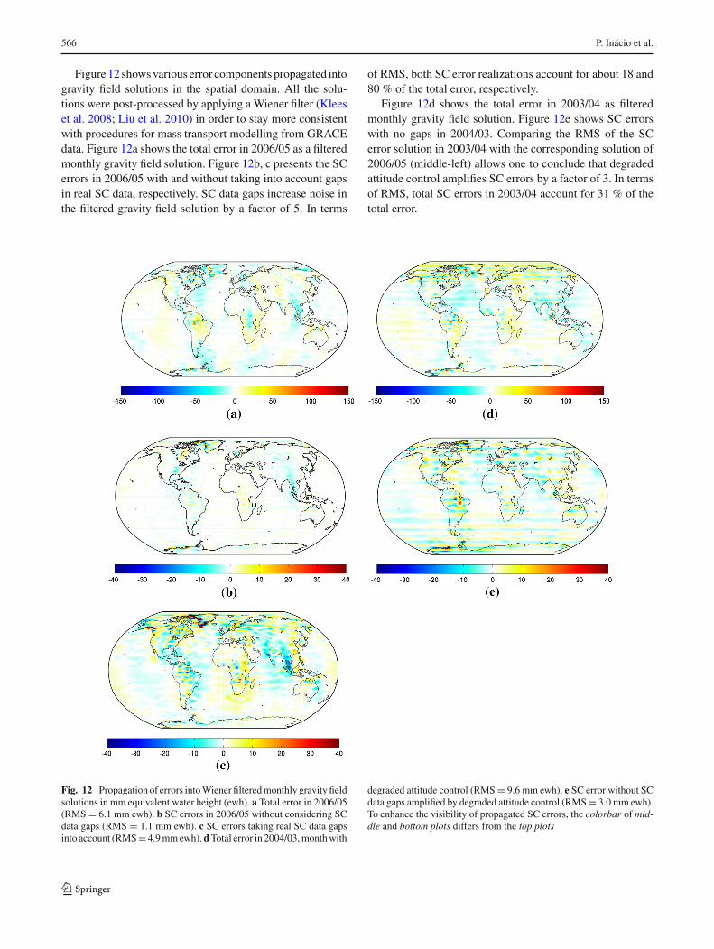
Figure 12 showsvarious error components propagated intogravity field solutions in the spatial domain. All the solu-tions were post-processed by applying a Wiener filter (Kleeset al. 2008; Liu et al. 2010) in order to stay more consistentwith procedures for mass transport modelling from GRACEdata. Figure 12a shows the total error in 2006/05 as a filteredmonthly gravity field solution. Figure 12b, c presents the SCerrors in 2006/05 with and without taking into account gapsin real SC data, respectively. SC data gaps increase noise inthe filtered gravity field solution by a factor of 5. In terms

of RMS, both SC error realizations account for about 18 and80 % of the total error, respectively.

Figure 12d shows the total error in 2003/04 as filteredmonthly gravity field solution. Figure 12e shows SC errorswith no gaps in 2004/03. Comparing the RMS of the SCerror solution in 2003/04 with the corresponding solution of2006/05 (middle-left) allows one to conclude that degradedattitude control amplifies SC errors by a factor of 3. In termsof RMS, total SC errors in 2003/04 account for 31 % of thetotal error.

Fig. 12 Propagation of errors intoWiener filteredmonthly gravity fieldsolutions in mm equivalent water height (ewh). a Total error in 2006/05(RMS = 6.1 mm ewh). b SC errors in 2006/05 without considering SCdata gaps (RMS = 1.1 mm ewh). c SC errors taking real SC data gapsinto account (RMS= 4.9mmewh).dTotal error in 2004/03,monthwith

degraded attitude control (RMS= 9.6 mm ewh). e SC error without SCdata gaps amplified by degraded attitude control (RMS= 3.0 mm ewh).To enhance the visibility of propagated SC errors, the colorbar of mid-dle and bottom plots differs from the top plots

123


The propagated SC errors in Fig. 12 are particularly highat places with significant geophysical signal, e.g. Greenland,Alaskan Glaciers,West Antarctica, etc. However, one shouldnot wrongly conclude attitude errors themselves are signifi-cantly stronger at these regions. Larger propagated errors inthese regions are caused by the use of theWiener filter to reg-ularize the monthly gravity field solutions. The Wiener filteris defined based on the covariance matrix of known masstransport signal over an extended period of time. As a con-sequence, the filter is more aggressive in regions with smallmass transport signal while it is more permissive in regionswith large mass transport signal. Figure 12 then shows howattitude errors propagate intoWiener filteredmonthly gravityfield models.

In Fig. 12b, c, e, SC errors propagate as horizontal stripes,a pattern already seen along the boresight axes of the SCerror estimates, cf., Fig. 2. This finding is consistent with theresults presented in Horwath et al. (2011). Similar horizontalstripes can also be observed in the total error solution of2003/04. This supports the conclusion that SC errors maybe a significant error source in the gravity field solution of2003/04.

7 Conclusions

We showed that the accuracy of the SCs cross-boresight axesis about 23 µrad which is close to the expected maximumof 24 µrad. In both satellites, the accuracy of the primaryboresight axis is significantly worse compared with the sec-ondary SC boresight axis. The ratio between the accuracy ofthe cross- and boresight axes matches the expected value of8, if we consider the secondary SC boresight axes. If we con-sider the primary SC boresight axis, than this ratio is higher,indicating that errors are stronger along these axes. The SCson board GRACE-A and GRACE-B have about the sameaccuracy except for the primary SC boresight axes, whereGRACE-A is less accurate.

We observed two distinct types of error in SCs on boardGRACE, i.e. random and harmonic. Harmonic errors arehighly correlated with the satellite’s true anomaly, indicat-ing that they are caused by the environment of the satelliteand not by the SC instruments themselves. We applied a cus-tom estimation method to extract both components from atime series containing large amounts of clustered gaps. Con-sidering different months, satellites and SCs, we showed thatharmonic errors have a higher standard deviation than sto-

chastic errors. In terms of PSD12 of ISA, the stochastic error

has a flat spectrum up to 10 mHz. The harmonic error isdominant in the frequency range 3–10 mHz.

SC errors alone account for about 18% of the total error interms of filtered gravity field solutions.We showed that these

errors are amplified in the presence of gaps in the SC dataand during periods of degraded attitude control. Under theseconditions, SC errors may become significant contributors tothe error budget of GRACE.

We showed that pitch and yaw errors are amplified by gapsin the SC data, which increase the anisotropy in the accuracyof the satellite attitudes. In terms of RMS of filtered gravityfield solutions, we showed that gaps in real SC data amplifySC errors by a factor of 5. This factor might even be largerfor months with bigger amount of gaps in the SC data.

For the period 2003–2010, we identified several monthswith degraded performance of the attitude control system:2010/06, 2005/12 and 2003/02 till 2003/05. A particularlybad month is 2003/04 when propagated attitude errors areamplified by a factor of 3 in terms of RMS of filtered gravityfield solution. In this monthly solution, SC errors account for31 % of total error without considering any gaps in the SCdata. The similarity between the spatial patterns of the twosolutions suggests that this number is, in reality, even higher.This shows that a degraded performance of the attitude con-trol system might have a significant impact on the quality ofmonthly GRACE solutions.

8 Discussion: attitude determination errors and futuresatellite gravimetry missions

Throughout this paper, we assumed that SC errors areobserved in the difference between the SC measurements,which only contain the differential SC error. Errors commonto both SCs are not observed. In fact, in this sense, we do notmodel the complete SC error, but only the differential part.However, it should be noticed that common SC errors arelikely of less concern. There could be two types of commonSC errors: time-invariant (static) common errors and time-variable (dynamic) common errors. Static common errorsare eliminated by calibration of the attitude system with on-ground and in-flightmanoeuvres, such that they are of no con-cern. Regarding dynamic common errors, one should keepin mind that each SC is an independent instrument makingindependent measurements; there is no obvious reason as towhy their measurements should have a significant commonerror.

To compute the SC error estimates, we make use of theQSA1Bproduct specifying the relative attitude between eachSC and the SRF. Despite of being accurately measured on-ground and calibratedwith in-flight manoeuvres, the QSA1Bproduct is not error free. However, errors in the QSA1B arenot fundamentally different from SC errors, and they areimplicitly considered in the SC error estimates.

In this publication, we follow the methodology devel-oped by Liu et al. (2010) to compute monthly gravity fieldsolutions from GRACE ISA. Other methodologies exist,

123


which instead make use of range and/or range-rate data.We believe, however, that our results are relevant indepen-dently of the chosen methodology. In one way or another,all methodologies use some form of KBR data, all conta-minated by errors in the geometric correction. The conver-sion of ranges into range-rates or range-accelerations canbe represented in the frequency domain as a multiplica-tion with iω and −ω2, respectively. Therefore, the signal-to-noise ratio at a given frequency would be the same forany type of observable. Furthermore, we employ a statis-tically optimal inversion scheme, which takes the depen-dence of noise on frequency into account. Consistent resultsmust be achieved for alternative methodologies, as longas they employ statistically optimal inversion schemes, nomatter whether ranges, range-rates, or range-accelerationsare used as input (Ditmar and van Eck van der Sluijs2004).

Reducing errors in the attitude product of GRACE andfuture satellite gravimetry missions could be achieved byincluding information provided by the accelerometers onboard the satellites. The accelerometers are able to mea-sure the rotation of the proof mass. These measurements canbe combined with SC data, potentially leading to improve-ments in attitude data in the high-frequency part of thespectrum. A similar approach has already been appliedin the GOCE mission for the fusion of attitude data col-lected by the star camera and the gradiometer instruments(Stummer et al. 2011; Frommknecht et al. 2011; Stummeret al. 2012). It should be investigated, however, whetherinformation collected by the accelerometers is accurateenough to substantially reduce noise in the attitude prod-ucts.

Errors in the roll angle are not critical for the purposesof gravity field modelling. The opposite is true for errorsin the pitch and yaw angles, which have a large impacton the antenna phase centre correction. We have shownthat the accuracy in the determination of the pitch and yawangles is worse than that of the roll angle. Furthermore,pitch and yaw errors are amplified by gaps in the SC data,while the errors in roll are only slightly worse. This leavesspace for an optimization of SC arrays in future low–lowsatellite-to-satellite tracking (ll-sst) gravity missions, so thatthe maximum accuracy for pitch and yaw angles is main-tained even in the periods when only one SC is operational.An example of how this setup could look like is shown inFig. 13. Because the roll angle determination is not criti-cal, both (less accurate) boresight axes are oriented in thex-axis direction ensuring the full accuracy of both SC’s forthe determination of the much more critical pitch and yawangles.

The cause of the harmonic error component in the SCmeasurements is not known to us. Further progress in SCdesign and data processing may reduce this error, which will

Fig. 13 Possible SC configuration based on the single fact that rollangle determination is not critical for gravity field recovery. Blue repre-sents x-, green represents y- and red represents z-axis, the least accurateboresight axis

also improve the accuracy of the satellite attitude determina-tion. Reducing the harmonic error may improve the signal-to-noise ratio in the range of 3–10 mHz, where most of infor-mation about time-variable gravity signal is located. In thisfrequency range, no other sources of errors have yet beenidentified. Understanding and mitigating all sources of errorin this range is of interest both forGRACEand future satellitegravity missions.

In our analysis, we focused on the propagation of SCerrors through the geometric correction of the KBR data.In the context of GRACE, this is likely the most critical wayin which these errors propagate into estimates of the time-varyinggravityfield. In the context of future gravitymissions,it is expected that they will make use of laser interferometersto measure inter-satellite ranges. The proposed architecturefor the laser interferometer of GRACE-FO places the virtualmeasurement point at the position of the accelerometer proofmass (Sheard et al. 2012). Such an architecture is insensitivetoSCerrors as it does not require a geometric correction at all.However, in view of a higher overall accuracy of GRACE-FO, additional studies may be required to understand thepropagation of attitude errors through the GNSS data andthrough theorientationof thenon-gravitational accelerations.Then, a proper understanding of SCerrors andhow theyprop-agate into the attitude are necessary.

Acknowledgments We would like to thank S. Bettadpur at the Cen-tre for Space Research of the University of Texas for providing us withtwo months of GRACE L1A SC data, T. Bandikova for providing herexpertise in the initial phase of our work, and Q. Zhao from the GNSSResearch and Engineering Centre of Wuhan University for providingus with the PANDA software for satellite orbit integration. We alsowould like to thank 3 anonymous reviewers and the editor J. Kusche formany valuable comments which helped us to improve the manuscript.The research was financially supported by the Netherlands Organiza-tion for Scientific Research (NWO), which is gratefully acknowledged.The research was also sponsored by the Stichting Nationale Faciliteiten(National Computing Facilities Foundation, NCF) by providing thehigh-performance computing facilities.

OpenAccess This article is distributed under the terms of theCreativeCommons Attribution License which permits any use, distribution, andreproduction in any medium, provided the original author(s) and thesource are credited.

123


Appendix A: Rotations

Relative orientations between two arbitrary reference framescan be defined as a set of three consecutive rotations. Con-sider the roll angle α, the pitch angle β and the yaw angle γ ,denoting rotations around the x-, y- and z-axes, respectively.This set of angles is also known as Cardan angles. We fol-low the zyx convention, stating the order and the axis alongwhich each of the intrinsic rotations is applied and we definerotations to be active transformations. Let Rb

a , be the matrixwhich rotates vectors from frame a into frame b, written as(Jekeli 2001),

Rba = Rz(γ )Ry(β)Rx (α)

=⎡

⎣cos γ − sin γ 0sin γ cos γ 00 0 1

⎤

⎦

⎡

⎣cosβ 0 sin β

0 1 0− sin β 0 cosβ

⎤

⎦

⎡

⎣1 0 00 cosα − sin α

0 sin α cosα

⎤

⎦

=⎡

⎣cos γ cosβ cos γ sin β sin α − sin γ cosα cos γ sin β cosα + sin γ sin α

sin γ cosβ sin γ sin β sin α + cos γ cosα sin γ sin β cosα − cos γ sin α

− sin β cosβ sin α cosβ cosα

⎤

⎦ . (27)

This type of matrix is known as direction cosine matrix(DCM). The DCM can also be represented as a vectorial

function R(ψ), whereψ ≡ [α β γ

]Tis an axial vector con-

sisting of the ordered triple of Cardan angles representing therotation between two arbitrary frames. Axial vectors are nottrue vectors because they do not fulfil all the properties ofvectors. It can be shown however (Jekeli (2001), [chap. 1])that for small rotation angles, axial vectors do behave like truevectors and under this assumption it becomes possible to add,subtract and rotate small rotation angles between differentreference frames. Assuming that ψ represents a small-anglerotation, Eq. (27), R(ψ) can be approximated to,

Rψ =⎡

⎣1 −γ β

γ 1 −α

−β α 1

⎤

⎦ = I − �, (28)

where,

� =⎡

⎣0 γ −β

−γ 0 α

β −α 0

⎤

⎦

The DCM, cf., Eqs. (27) and (28), are orthogonal matrices,with the property that,

Rba

(Rba

)T = I ⇒ Rab =

(Rba

)−1 =(Rba

)T. (29)

Multiplication of a given vector va defined in frame a withmatrix Rb

a transforms it to frame b,

vb = Rbav

a, (30)

and for a given tensor Aa defined in frame a, the followingoperation also transforms it to frame b,

Ab = RbaA

aRab . (31)

Consecutive rotations are achieved by successive multiplica-tion of rotations matrices, as seen in Eq. (27),

Rca = Rc

bRba . (32)

Appendix B: Optimal SC combination

In this Appendix, we formulate the combination of multi-ple SC measurements, on board a single satellite. The resultof this method is the set of Cardan angles which minimizesthe square differences w.r.t. all SC measurements. Further-more, this combination also takes into account the inherentanisotropy of the SC instruments. This combination is origi-nally presented in Romans (2003) in terms of attitude quater-nions.

In the presence of multiple SCs, one wishes to combineall measurements in an optimal manner. Let εψ,opt be theset of small-angle rotations which minimizes the differencesw.r.t. the errors in all SCs. It is obtained by minimizing thequadratic error function J ,

J =∑

i

(εSiψ,opt − ε

Siψ,i

)T�i

(εSiψ,opt − ε

Siψ,i

), (33)

where εψ,i ≡ [εα,i εβ,i εγ,i

]Tis the vector representing the

errors in the roll (εα,i ), pitch (εβ,i ) and yaw (εγ,i ) angles inthe rotation measured by the i-th star camera and �i is theinverse of the covariance matrix or information matrix,

�i = C−1i (34)

123


Equation (5) shows that, for small measurement errors, thedifferential rotation between any pair of SCs is linearlydependent on the error of each SC. This allows us to writean expression for the errors in each SC w.r.t. a single one,

εCψ, j = εCψ,1 − �εCψ,1 j . (35)

Let �Ci ≡ RC

Si�i R

SiC be the information matrix rotated to

the C-frame. The cost function can be written in the C-frameas,

J =∑

i

(εCψ,opt − εCψ,i

)T�C

i

(εCψ,opt − εCψ,i

). (36)

With N SC measurements, minimization of J would requirethe knowledge of the errors εψ,i in each SC measurement.This knowledge is not available, so we must tackle the prob-lem differently using the differences between pairs of SCmeasurements. Let us choose the first star camera, i = 1,and making use of Eq. (35), one can relate all SC errors tothis one, so that the objective function becomes,

J =∑

i

(εCψ,opt − εCψ,1 + �εCψ,1i

)T

�Ci

(εCψ,opt − εCψ,1 + �εCψ,1i

), (37)

where,

�εCψ,11 = 0

Let εopt ≡ εCψ,opt−εCψ,1, be defined as the optimal correctionto the first SC measurement. One can rewrite,

J =∑

i

(εopt + �εCψ,1i

)T�C

i


),

= εopt�C1 εopt +

∑

i �=1


)T

�Ci


). (38)

Minimization of the cost function J w.r.t. εopt yields,

εopt = −(�C

total

)−1 ∑

i �=1

�Ci �εCψ,1i , (39)

where �Ctotal = ∑

i �Ci . It can be shown that the solution

does not depend on the choice of the camera w.r.t. which allerrors are defined in Eq. (37).

The optimal combination of multiple SCmeasurements isthen obtained by applying the optimal correction εopt to themeasurement of the first one,

RCI,opt = R(εopt) RC

I,1. (40)

References

Bandikova T, Flury J, Ko UD (2012) Characteristics and accuraciesof the GRACE inter-satellite pointing. Adv Sp Res 50:123–135.doi:10.1016/j.asr.2012.03.011

Bender P, Hall J, Ye J, Klipstein W (2003) Satellite–satellite laser linksfor future gravity missions. Sp Sci Rev 108(1–2):377–384. doi:10.1023/A:1026195913558

Case K, Kruizinga G,Wu SC (2010) GRACE level-1b data product userhandbook. Tech. Rep. JPL D-22027, Jet Propulsion Laboratory

Davis E, Dunn C, Stanton R, Thomas J (1999) The GRACE mis-sion: Meeting the technical challenges. Tech. Rep. IAF-99-I3.2.05, Jet Propulsion Laboratory. http://hdl.handle.net/2014/18091. Accessed Mar 2014

Dehne M, Cervantes FG, Sheard B, Heinzel G, Danzmann K (2009)Laser interferometer for spaceborne mapping of the earth’s gravityfield. J Phys Conf Ser 154(012):023. doi:10.1088/1742-6596/154/1/012023

Ditmar P, van Eck van der Sluijs AA (2004) A technique for modelingthe Earth’s gravity field on the basis of satellite accelerations. JGeod 78:12–33. doi:10.1007/s00190-003-0362-1

Ditmar P, Teixeira da Encarnação J, Farahani HH (2012) Understandingdata noise in gravity field recovery on the basis of inter-satelliterangingmeasurements acquired by the satellite gravimetrymissionGRACE. J Geod 87(9):1–25. doi:10.1007/s00190-011-0531-6

Drinkwater MR, Haagmans R, Muzi DA, Popescu A, FloberghagenR, Kernand M, Fehringer M (2007) The GOCE gravity mission:ESA’s first core earth explorer. In: Proceedings of 3rd InternationalGOCE User Workshop, 6–8 November, 2006, Frascati, Italy, ESASpecial Publication, SP-627, ISBN 92-9092-938-3, pp. 1–8

Farahani HH (2013)Modelling the Earth’s static and time-varying grav-ity field using a combination of GRACE and GOCE data. Ph.D.thesis, Delft University of Technology

Farahani HH, Ditmar P, Klees R (2013a) Assessment of the added valueof data from the GOCE satellite mission to time-varying grav-ity field modelling. J Geod 88(2):1–22. doi:10.1007/s00190-013-0674-8

Farahani HH, Ditmar P, Klees R, Liu X, Zhao Q, Guo J (2013b) Thestatic gravity field model DGM-1S fromGRACE and GOCE data:computation, validation and an analysis of GOCE missions addedvalue. J Geod 87(9):843–867. doi:10.1007/s00190-013-0650-3

Flechtner F, Dobslaw H, Fagiolini E (2014) AOD1B Product Descrip-tion Document for Product Release 05. Tech. Rep. GRACE327–750, GFZ German Research Centre for Geosciences.http://www.gfz-potsdam.de/fileadmin/gfz/sec12/pdf/GRACE/AOD1B/AOD1B_20140520.pdf. Accessed Mar 2014

Frommknecht B, Lamarre D, Meloni M, Bigazzi A, Floberghagen R(2011) GOCE level 1b data processing. J Geod 85(11):759–775.doi:10.1007/s00190-011-0497-4

Herman J, Presti D, Codazzi A, Belle C (2004) Attitude controlfor GRACE. In: 18th International Symposium on Space FlightDynamics, ESA Special Publication, vol 548, p 27

Horwath M, Lemoine JM, Biancale R, Bourgogne S (2011) ImprovedGRACE science results after adjustment of geometric biases in theLevel-1b K-band ranging data. J Geod 85(1):23–38. doi:10.1007/s00190-010-0414-2

Jekeli C (2001) Inertial navigation systems with geodetic applications.Walter de Gruyter, Berlin

Kang Z, Tapley B, Bettadpur S, Ries J, Nagel P, Pastor R (2006) Preciseorbit determination for the GRACE mission using only GPS data.J Geod 80(6):322–331. doi:10.1007/s00190-006-0073-5

Kim J (2000) Simulation study of a low–low satellite-to-satellite track-ing mission. Ph.D. thesis, University of Texas at Austin

KleesR,DitmarP,BroersenP (2003)How tohandle coloredobservationnoise in large least-squares problems. J Geod 76(11–12):629–640.doi:10.1007/s00190-002-0291-4

123

http://dx.doi.org/10.1016/j.asr.2012.03.011

http://dx.doi.org/10.1023/A:1026195913558

http://dx.doi.org/10.1023/A:1026195913558

http://hdl.handle.net/2014/18091

http://hdl.handle.net/2014/18091

http://dx.doi.org/10.1088/1742-6596/154/1/012023

http://dx.doi.org/10.1088/1742-6596/154/1/012023

http://dx.doi.org/10.1007/s00190-003-0362-1

http://dx.doi.org/10.1007/s00190-011-0531-6

http://dx.doi.org/10.1007/s00190-013-0674-8

http://dx.doi.org/10.1007/s00190-013-0674-8

http://dx.doi.org/10.1007/s00190-013-0650-3

http://www.gfz-potsdam.de/fileadmin/gfz/sec12/pdf/GRACE/AOD1B/AOD1B_20140520.pdf

http://www.gfz-potsdam.de/fileadmin/gfz/sec12/pdf/GRACE/AOD1B/AOD1B_20140520.pdf

http://dx.doi.org/10.1007/s00190-011-0497-4

http://dx.doi.org/10.1007/s00190-010-0414-2

http://dx.doi.org/10.1007/s00190-010-0414-2

http://dx.doi.org/10.1007/s00190-006-0073-5

http://dx.doi.org/10.1007/s00190-002-0291-4


Klees R, Revtova E, Gunter B, Ditmar P, Oudman E, Winsemius H,Savenije H (2008) The design of an optimal filter for monthlyGRACE gravity models. Geophys J Int 175(2):417–432. doi:10.1111/j.1365-246X.2008.03922.x

Kruizinga G, Bertiger W, Finch C, Kuang D, Watkins M, Yuan DN,Bettadpur S, Wang F (2010) GRACE Level-1 Status. In: GRACEScience Team Meeting 2010. https://media.gfz-potsdam.de/gfz/sec12/GSTM-2010/GSTM2010-A0.zip. Accessed Mar 2014

LiebeC (2002)Accuracy performance of star trackers—a tutorial. IEEETrans Aerosp Electron Syst 38:587–599

Liu X, Ditmar P, Siemes C, Slobbe DC, Revtova E, Klees R, Riva R,Zhao Q (2010) DEOS mass transport model (DMT-1) based onGRACE satellite data: methodology and validation. Geophys J Int181(2):769–788. doi:10.1111/j.1365-246X.2010.04533.x

Pail R (2005) A parametric study on the impact of satellite attitudeerrors on GOCE gravity field recovery. J Geod 79(4–5):231–241.doi:10.1007/s00190-005-0464-z

Romans L (2003) Optimal combination of quaternions from multi-ple star cameras. JPL Internal Memorandum, Jet Propulsion Lab-oratory. ftp://podaac.jpl.nasa.gov/allData/grace/docs/quaternion_memo.pdf. Accessed Mar 2014

Savcenko R, Bosch W (2012) EOT11a - empirical ocean tidemodel from multi-mission satellite altimetry. Tech. Rep.89, DGFI. http://www.dgfi.badw.de/fileadmin/docs/dgfi_reports/DGFI_Report_89.pdf. Accessed Mar 2014

Schmidt R, Flechtner F, Meyer U, Neumayer H, Dahle C, Konig R,Kusche J (2008) Hydrological signals observed by the GRACEsatellites. Surv Geophys 29:319–334. doi:10.1007/s10712-008-9033-3

Sheard BS, Heinzel G, Danzmann K, Shaddock DA, Klipstein WM,Folkner WM (2012) Intersatellite laser ranging instrument for theGRACE follow-on mission. J Geod 86(12):1083–1095. doi:10.1007/s00190-012-0566-3

Stummer C, Fecher T, Pail R (2011) Alternative method for angular ratedetermination within the GOCE gradiometer processing. J Geod85(9):585–596. doi:10.1007/s00190-011-0461-3

Stummer C, Siemes C, Pail R, Frommknecht B, Floberghagen R (2012)Upgrade of the GOCE level 1b gradiometer processor. Adv Sp Res49(4):739–752. doi:10.1016/j.asr.2011.11.027

Tapley BD, Bettadpur S, Ries JC, Thompson PF, Watkins MM (2004)GRACE measurements of mass variability in the earth system.Science 305(5683):503–505. doi:10.1126/science.1099192

Tikhonov A, Arsenin VY (1977) Solutions of ill-posed problems. WHWinston, Washington, DC 330

Wu SC, Kruizinga G, Bertinger W (2006) Algorithm Theoretical BasisDocument forGRACELevel-1BData ProcessingV1.2. Tech.Rep.JPL D-27672, Jet Propulsion Laboratory

123

http://dx.doi.org/10.1111/j.1365-246X.2008.03922.x


https://media.gfz-potsdam.de/gfz/sec12/GSTM-2010/GSTM2010-A0.zip

https://media.gfz-potsdam.de/gfz/sec12/GSTM-2010/GSTM2010-A0.zip


http://dx.doi.org/10.1007/s00190-005-0464-z

ftp://podaac.jpl.nasa.gov/allData/grace/docs/quaternion_memo.pdf

ftp://podaac.jpl.nasa.gov/allData/grace/docs/quaternion_memo.pdf

http://www.dgfi.badw.de/fileadmin/docs/dgfi_reports/DGFI_Report_89.pdf

http://www.dgfi.badw.de/fileadmin/docs/dgfi_reports/DGFI_Report_89.pdf

http://dx.doi.org/10.1007/s10712-008-9033-3

http://dx.doi.org/10.1007/s10712-008-9033-3

http://dx.doi.org/10.1007/s00190-012-0566-3

http://dx.doi.org/10.1007/s00190-012-0566-3

http://dx.doi.org/10.1007/s00190-011-0461-3

http://dx.doi.org/10.1016/j.asr.2011.11.027

http://dx.doi.org/10.1126/science.1099192

Documents

Analysis of star camera errors in GRACE data and their