Analysis of Rotational Deformations from Directional

Data

Jorn Schulz1, Sungkyu Jung2, Stephan Huckemann3,

Michael Pierrynowski4, J. S. Marron5 and Stephen M. Pizer5

1University of Tromsø, 2University of Pittsburgh, 3University of Gottingen,

4McMaster University, Hamilton 5University of North Carolina at Chapel Hill

March 26, 2014

Abstract

This paper discusses a novel framework to analyze rotational deformations of real

3D objects. The rotational deformations such as twisting or bending have been ob-

served as the major variation in some medical applications, where the features of the

deformed 3D objects are directional data. We propose modeling and estimation of

the global deformations in terms of generalized rotations of directions. The proposed

method can be cast as a generalized small circle fitting on the unit sphere. We also

discuss the estimation of descriptors for more complex deformations composed of two

simple deformations. The proposed method can be used for a number of different 3D

object models. Two analyses of 3D object data are presented in detail: one using

skeletal representations in medical image analysis as well as one from biomechanical

gait analysis of the knee joint. Supplementary Materials are available online.

Keywords: 3D object, axis of rotation, directional statistics, skeletal model, small circle.

1 Introduction

Modeling deformations of a real object is a central issue in computer vision, biomechanics

and medical imaging. In a number of applications, generalized rotations appear to be the

major forms of deformation. For instance, the major variation of shapes of hippocampi

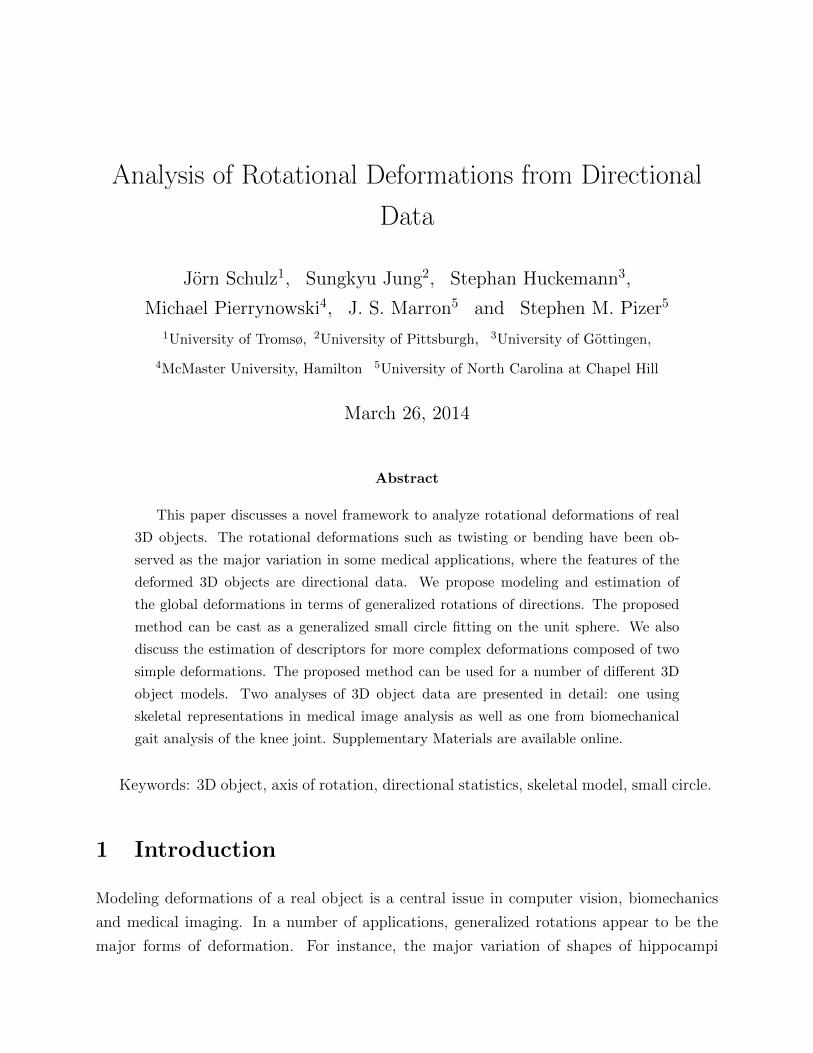
(a) (b) (c)

Figure 1: 3D objects and their models. (a) S-rep of a hippocampus (b) S-rep of a rotationallydeformed ellipsoid. (c) Attached boundary normals on the meshed surface of an ellipsoid.

in the human brain has been shown to be bending of the object (Joshi et al., 2002; Pizer

et al., 2013); Human joint movements, such as the motion of the knee or the elbow, consist

of bending and twisting about the joint (Rivest, 2001; Rivest et al., 2008; Oualkacha and

Rivest, 2012). A direct modeling of such rotational deformations will promote a precise

description of object variation and will be important for surgery or treatment planning.

In this paper, we propose an estimation procedure for descriptors of underlying rotational

deformations from a random sample of objects. Specifically, the descriptors are parameters

of the model we introduce in Section 2; they include rotational axes of a rotational model.

Our model embraces a number of different types of deformations including rigid rotation,

bending, twisting and a mixture of the last two. Although we aim to analyze variations

in sophisticated human organs such as the hippocampus (Fig. 1a), we work with a simpler

object resembling ellipsoids (Fig. 1b) to show the validity of the proposed method.

A major challenge in modeling rotational deformation is that such variations are typically

mixed with translational and scaling effects. We address this issue by only considering

direction vectors, which are invariant to translation and size changes. It will be shown

that the rotational deformation can be sufficiently modeled using directional data. Another

advantage of our approach is that well-studied directional data techniques can be applied

(Fisher et al., 1993; Mardia and Jupp, 2000; Chang and Rivest, 2001; Jung et al., 2011).

Before we introduce our method, we point out several modeling approaches of 3D objects

that are relevant to our framework of directional data, as follows:

Point distribution model A solid object is modeled by the positions of the sampled sur-

face points on which directions normal to the surface can be attached (Cootes et al.,

1992; Dryden and Mardia, 1998; Kurtek et al., 2011). See Fig. 1c.

2

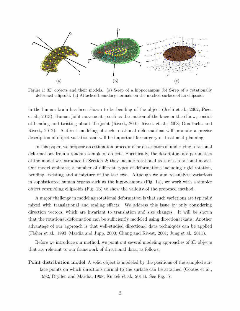
(a) A simple 3D object (b) Direction vectors

Figure 2: Toy example. (a) A toy object, to be deformed. (b) Each direction vector is a point onthe surface of the unit sphere.

Large deformations The shape changes of an object in images are modeled by the defor-

mations of a template image (Pennec, 2008; Rohde et al., 2008). The deformation can

be understood as a vector field, where each vector contains the direction.

S-rep In skeletal representations (s-rep), a 3D object is modeled by skeletal positions lying

inside of the object and spoke vectors pointing to the boundary of the object (Siddiqi

and Pizer, 2008; Pizer et al., 2013). See Fig. 1a and Fig. 1b. We describe s-rep data

analysis in more detail in Section 5.

In all three cases, the direction vectors are predetermined by the shape models.

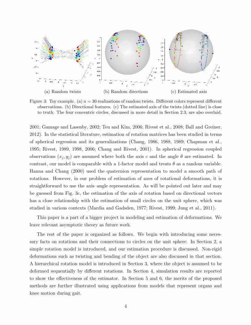
The framework of our analysis can be understood by considering a simple example of a

3D object (Fig. 2). The object is modeled by four surface points (or skeletal positions) with

attached direction vectors µj for 1 ≤ j ≤ 4 (Fig. 2a). Consider random twists of the object,

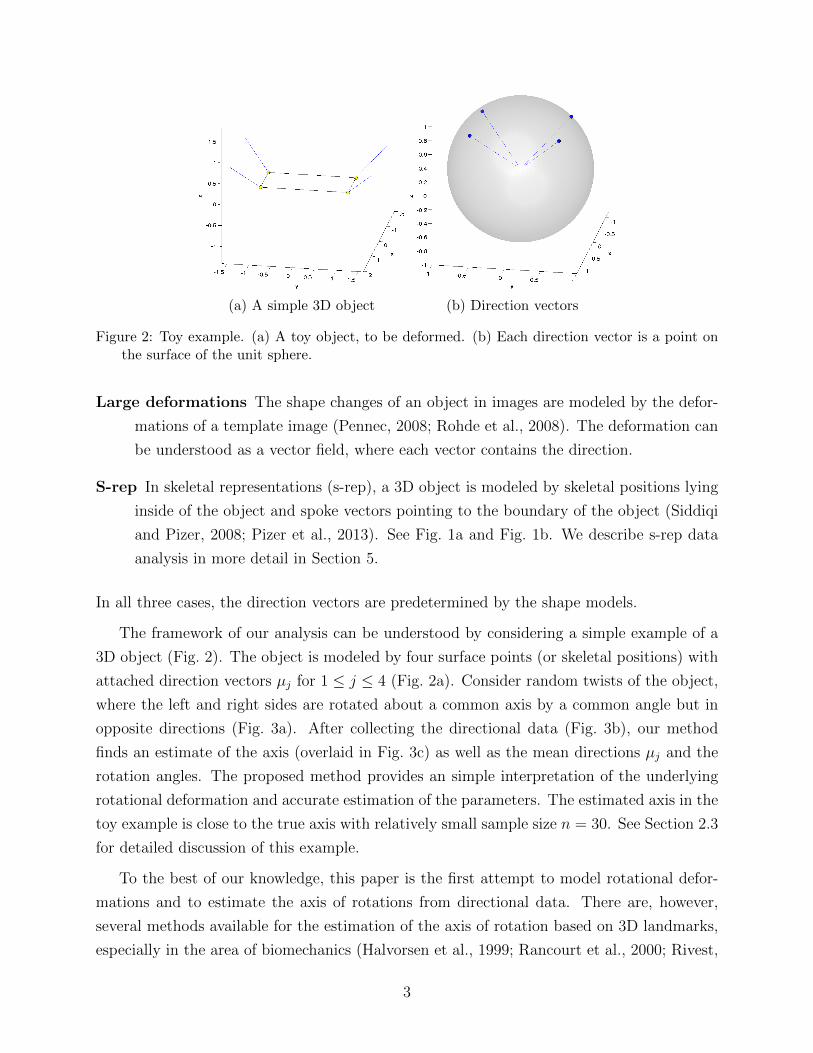
where the left and right sides are rotated about a common axis by a common angle but in

opposite directions (Fig. 3a). After collecting the directional data (Fig. 3b), our method

finds an estimate of the axis (overlaid in Fig. 3c) as well as the mean directions µj and the

rotation angles. The proposed method provides an simple interpretation of the underlying

rotational deformation and accurate estimation of the parameters. The estimated axis in the

toy example is close to the true axis with relatively small sample size n = 30. See Section 2.3

for detailed discussion of this example.

To the best of our knowledge, this paper is the first attempt to model rotational defor-

mations and to estimate the axis of rotations from directional data. There are, however,

several methods available for the estimation of the axis of rotation based on 3D landmarks,

especially in the area of biomechanics (Halvorsen et al., 1999; Rancourt et al., 2000; Rivest,

3

(a) Random twists (b) Random directions (c) Estimated axis

Figure 3: Toy example. (a) n = 30 realizations of random twists. Different colors represent differentobservations. (b) Directional features. (c) The estimated axis of the twists (dotted line) is closeto truth. The four concentric circles, discussed in more detail in Section 2.3, are also overlaid.

2001; Gamage and Lasenby, 2002; Teu and Kim, 2006; Rivest et al., 2008; Ball and Greiner,

2012). In the statistical literature, estimation of rotation matrices has been studied in terms

of spherical regression and its generalizations (Chang, 1986, 1988, 1989; Chapman et al.,

1995; Rivest, 1989, 1998, 2006; Chang and Rivest, 2001). In spherical regression coupled

observations (xj, yj) are assumed where both the axis c and the angle θ are estimated. In

contrast, our model is comparable with a 1-factor model and treats θ as a random variable.

Hanna and Chang (2000) used the quaternion representation to model a smooth path of

rotations. However, in our problem of estimation of axes of rotational deformations, it is

straightforward to use the axis–angle representation. As will be pointed out later and may

be guessed from Fig. 3c, the estimation of the axis of rotation based on directional vectors

has a close relationship with the estimation of small circles on the unit sphere, which was

studied in various contexts (Mardia and Gadsden, 1977; Rivest, 1999; Jung et al., 2011).

This paper is a part of a bigger project in modeling and estimation of deformations. We

leave relevant asymptotic theory as future work.

The rest of the paper is organized as follows. We begin with introducing some neces-

sary facts on rotations and their connections to circles on the unit sphere. In Section 2, a

simple rotation model is introduced, and our estimation procedure is discussed. Non-rigid

deformations such as twisting and bending of the object are also discussed in that section.

A hierarchical rotation model is introduced in Section 3, where the object is assumed to be

deformed sequentially by different rotations. In Section 4, simulation results are reported

to show the effectiveness of the estimator. In Section 5 and 6, the merits of the proposed

methods are further illustrated using applications from models that represent organs and

knee motion during gait.

4

1.1 Rotations, circles and spheres

In the axis–angle representation of rotations, an axis c is the unit vector that is left fixed

by the rotation and an angle θ gives the amount of rotation. A unit vector lies on the unit

sphere S2 = {x ∈ R3 : ‖x‖ = 1}. The axis–angle pair (c, θ) ∈ S2 × [0, 2π) represents a

rotation in 3-space, where a vector x ∈ R3 is rotated by (c, θ) by applying x 7→ R(c, θ)x with

R(c, θ) = I3 + sin θ[c]× + (1− cos θ)(cc′ − I3), (1)

where c′ denotes the transpose of c, and [c]× is the cross product matrix satisfying [c]×v = c×vfor any v ∈ R3.

A useful observation in our analysis is that the direction vectors follow circles when they

are rotated. In particular, when x ∈ S2 is rotated about an axis c ∈ S2, the trajectory of

such rotation is precisely a circle δ(c, r) = {x ∈ S2 : x′c = cos(r)} ⊂ S2, which is a set of

equidistant points from c. We call c the center and r = arccos(x′c) the radius of the circle.

Since δ(c, r) = δ(−c, π − r) we may assume that r ≤ π/2. We call δ(c, r) a great circle if

r = π/2 and a small circle if r < π/2.

If a K-tuple of K ≥ 2 direction vectors x = (x1, . . . , xK) ∈ (S2)K are rotated together

about a common axis c, then each of the rotated direction vectors is on a circle with common

center c but with different radii rj = arccos(c′xj), j = 1, . . . , K. Denote the collection of

concentric circles with a common center c and radii tuple r = (r1, . . . , rK) ∈ [0, π/2] ×[0, π]K−1 by

δ(c, r) = {(x1, . . . , xK) ∈ (S2)K : x′jc = cos(rj), j = 1, . . . , K}.

To work with observations on S2, the geodesic distance function dg : S2 × S2 → [0, π]

is defined by the arc length of the shortest great circle segment joining x, y ∈ S2, and is

dg(x, y) = arccos(x′y). We further define dg(x,A) = infy∈A dg(x, y) for x ∈ S2, A ⊂ S2. For

a random element X whose domain is S2, a sensible notion of mean µ(X) is defined by a

minimizer of mean squared distance,

µ(X) = argminx∈S2

E{d2g(x,X)},

often called the geodesic or Frechet mean (Frechet, 1948; Karcher, 1977; Huckemann, 2012).

A useful measure of dispersion is the geodesic variance which is defined as Var(X) =

E{d2g(µ(X), X)} = minx∈S2 E{d2g(x,X)} provided that µ(X) exists.

5

2 Single rotational deformations

In this section, an estimation procedure for rotational deformation models is proposed. We

begin with a discussion on the simpler rigid rotation model.

2.1 Rigid rotation model

Suppose we have a K-tuple of random direction vectors X = (X1, . . . , XK). For some

unknown constants c, µj ∈ S2 and a latent random variable θ ∈ [−π/2, π/2), we model

Xj ∈ S2 (j = 1, . . . , K) as noisy observations of rotations of µj by R(c, θ), that is,

Xj = R(c, θ)µj ⊕ εj (j = 1, . . . , K). (2)

Here, the εj are independently distributed random error terms, and the ⊕ sign defines a

specific action of the error distribution as defined in the following.

There are several ways to define random spherical points X ∼ µ⊕ ε ∈ S2. A natural way

is to introduce an S2-valued distribution, e.g., the von Mises–Fisher distribution (Mardia

and Jupp, 2000, p. 36) with the density fvMF(x;µ, κ) ∝ exp(κµ′x) with respect to the

uniform measure on S2 for µ ∈ S2, κ > 0. Alternatively, one can utilize the tangent space at

µ ∈ S2, allowing a distribution on the tangent space to be mapped to S2. Another approach

is to use the embedding of S2 into R3, by scaling a three-dimensional random vector to

unit length. This approach is often called a perturbation model (Goodall, 1991). It is well-

known that a perturbation model introduces a bias in the estimation of the geodesic mean

unless the distribution is isotropic (Kent and Mardia, 1997; Le, 1998; Huckemann, 2011a).

In this paper in Section 4, we use the von Mises–Fisher distribution and in Section 5 the

perturbation model. In the following discussion, we do not specify a particular distribution

for ε, but require that the geodesic mean of X ∼ µ ⊕ ε is uniquely found at µ, i.e., µ =

argminx E{d2g(x,X)}. The geodesic variance Var(ε) := Var(µ⊕ ε) is then well defined.

In model (2), several different combinations of θ and µj lead to the same model. Specif-

ically, replacing θ and µj by θ∗(a) = θ − a and µ∗j(a) = R(c, a)µj for any a ∈ R gives the

same model as (2). Therefore, we assume

Eθ = 0. (3)

The trajectory of rotated direction vectors forms a small circle (cf. Section 1.1), which

is approximately true in the presence of the noise. In other words, the collection of Xj in

6

(2) are distributed along concentric circles with common center at c, as the following lemma

states.

Lemma 1. Let the η-neighborhood of concentric circles δ(c, r) be

δη(c, r) = {(X1, . . . , XK) ∈ (S2)K : dg(δ(c, rj), xj) < η for all j = 1, . . . , K},

for η > 0. If µ ⊕ εj are independent and identically distributed and spherically symmetric

about µ, then

P{X ∈ δη(c, r)} ≥{

1− Var(ε)

η2

}K.

The auxiliary parameters rj = arccos(c′µj) represent the radii of the concentric circles,

and are obtained from c and µj, the parameters of (2). A proof of Lemma 1 is given in the

Appendix.

Lemma 1 suggests that X and δ(c, r) are close with high probability, which motivates to

define the population concentric circles δ(c0, r0) as a minimizer of squared loss. In the view

of this estimation strategy, the capability of identifying parameters as minimizers leads to a

natural estimation strategy, namely the M–estimation or the sample Frechet mean (Karcher,

1977; Huckemann, 2011b). The rest of this section is devoted to the identification of the

population parameters c, rj and µj as population Frechet means.

First, the distance function ρ between δ(c, r) and x is defined as the Cartesian product

metric based on dg by

ρ2(δ(c, r),x) =K∑j=1

d2g (δ(c, rj), xj) =K∑j=1

(arccos(x′jc)− rj

)2.

The collection of population concentric circles δ(c0, r0) is defined as the Frechet ρ-mean set

argminc∈S2,r∈[0,π/2]×[0,π]K−1

Eρ2(δ(c, r),X), (4)

where the expectation E is with respect to the random directions X. We assume in the

following that there is a unique minimizer δ(c0, r0). The center c0 of the circles also represents

the axis of rotation.

It should be noted that there is no guarantee for the true axis of rotation c of (2) to be

the same as c0 from (4). Simulation studies, reported in the Supplementary Material, have

suggested that the case c0 = c occurs when Var(rjθj) is large enough compared to the error

variance Var(εj) for all j. In our simulation studies in Section 4, the effect of this bias is

7

shown to be small.

While the axis of rotation c is the center of the concentric circles δ(c, r), each base point

µj is also a point on δ(c, rj), j = 1, . . . , K. The assumption of isotropy of εj implies that

µ(Y θ0j ) = R(c, θ0)µj

for Y θ0j = R(c, θ0)µj+εj with deterministic angle θ0 ∈ [−π/2, π/2). In particular, µ(Y 0

j ) = µj.

For random θ define

µ(Xj|θ) := R(c, θ)µj .

With the distance function ρδ(c,r)(x, y) which measures the shortest arc-length between x, y ∈δ(c, r) along the (small) circle via ρδ(c,r)(x, y) = sin(r) arccos[(x′y − cos2(r))/sin2(r)] (Jung

et al., 2012) we have by definition

ψ0 = argminψ∈[−π/2,π/2)

Eρ2δ(c,rj)(µ(Xj|θ), R(c, ψ)µj) = argminψ∈[−π/2,π/2)

E(θ − ψ)2,

which leads to the minimizer ψ0 = 0 due to the assumption (3). Thus,

µj = argminµ∈δ(c,rj)

Eρ2δ(c,rj)(µ(Xj|θ), µ). (5)

Finally, we view µ(Xj|θ) as the expectation of Xj conditioned on the unobserved ran-

dom variable θ which represents the amount of rotation. Then, by solving the equation

µ(Xj|θ) = R(c, θ)µj for θ, using the Rodrigues’ rotation formula (Gray, 1980; Altmann,

2005) R(c, θ)µj = µj cos θ + (c× µj) sin θ + 〈c, µj〉c(1− cos θ), we get

θ = atan2[〈µ(Xj|θ), c× µj〉, 〈µ(Xj|θ), µj − c cos(rj)〉], (j = 1, . . . , K), (6)

where the two argument function atan2(x2, x1) ∈ (−π, π] is the signed angle between two

vectors e1 = (1, 0) and (x1, x2) ∈ R2.

2.2 Estimation

Suppose we have n independent observations X1, . . . ,Xn from model (2). Each Xi is a col-

lection of K directions Xi = (Xij)j=1,...,K . The estimates of parameters c, rj, µj are obtained

8

as the sample Frechet means as follows:

(c, r) = argminc,r1,...,rK

n∑i=1

K∑j=1

d2g{δ(c, rj), Xij}, (7)

µj = argminµ

n∑i=1

ρ2δ(c,rj)(P(c,rj)Xij, µ) (j = 1, . . . , K). (8)

Note that in (8), we have used P(c,rj)Xij, the projection of Xij onto δ(c, rj), instead of

E(Xij|θi) used in (5). The projection Pδ(c,r)x is a point on δ(c, r) with the minimal geodesic

distance to x, given by (Mardia and Gadsden, 1977, Eq. (3.3))

Pδ(c,r)x = argminv∈δ(c,r)

dg(v, x) =x sin(r) + c sin{dg(x, c)− r}

sin{dg(x, c)}.

The predicted values of the latent variable θi are obtained using (6) by substituting the

estimates for the parameters. The predictor for θi is θi = K−1∑K

j=1 θij for each i = 1, . . . , n

with

θij = atan2{〈P(c,rj)Xij, c× µj〉, 〈P(c,rj)Xij, µj − c cos(rj)〉}. (9)

Note that (8) and (9) lead to∑n

i=1 θij = 0 (j = 1, . . . , K), which is an empirical statement

of (3).

The least squares problems (7-8) do not have closed form solutions. The problem (8) is

simpler and the same as finding the geodesic mean of angles, since both P(c,rj)Xij and µ are

on the one-dimensional circle δ(c, rj). Solutions to this type of problem are combinatorial

(Moakher, 2002) but also found efficiently by numerical methods (Le, 2001; Fletcher et al.,

2003). The problem (7) is precisely the fitting of concentric (small) circles. Therefore,

numerical algorithms for (7) are generalized algorithms of the well-studied fitting of small

circles (Mardia and Gadsden, 1977; Rivest, 1999; Jung et al., 2011, 2012) and are discussed

in the Appendix.

2.3 Rotational deformations

The single rotation model (2) describes rigid rotations of objects. We extend the model

to more general cases so that the generalized rotational model can explain, for example,

non-rigid twisting or bending.

Suppose two direction vectors x1 and x2 are rotated about the same axis c but by different

angles θ1 and θ2. This allows the underlying object to deform. In general, the assumption of

9

a single rotation angle θ in (2) is relaxed to possibly different angles θ1, . . . , θK , which may

be either independent or dependent of each other. To incorporate such general situations,

the single rotation model is generalized to

Xj = R(c, θj)µj ⊕ εj (j = 1, . . . , K). (10)

The relationships among the θj can be specified using prior knowledge about the specific

rotational deformation. As a special case, when a rigid rotation is assumed, it is reasonable

to set θ1 = · · · = θK , which goes back to the model (2). The general model (10) includes

other important physical deformations. The twisting or bending of the object can be modeled

by different rotations with a common axis of rotation. As an example, when an object (and

its attached direction vectors) is twisted, one group of direction vectors is rotated clockwise,

while the other group is rotated counter–clockwise. Let I1 and I2 be a partition of the

indices {1, . . . , K} representing groups of the direction vectors that rotate together. A simple

twisting or bending motion can be obtained by assuming θj1 = −θj2 for all j1 ∈ I1, j2 ∈ I2.Another example is the scenario of independent rotations where all directions in the same

group rotate together (θj1 = θj2 , j1, j2 ∈ Il) but two angles in different groups are independent

(θj1 and θj2 are independent for j1 ∈ Il, j2 ∈ Ik, 1 ≤ l 6= k ≤ 2).

In all cases above, we assume that some functions fj are known in advance, so that the

relationships between θj are modeled through known functions, i.e., θj = fj(θ). Due to the

identifiability issue, which leads to the assumption (3), we assume E(θj) = 0.

In the estimation of the parameters in (10), we use the fact that the estimation procedure

(7) does not depend on specific assumptions of the latent variable θj. Therefore, the same

least squares estimators {c, rj, µj} can be used to estimate the parameters of (10). When

fj(θ) is known and invertible, the prediction of the ith sample of θ, θ(i), can be obtained.

Since each θij of (9) is a perturbed version of fj(θi), the prediction of θ(i) is then

θi =1

K

K∑j=1

f−1j (θij).

Remark 1. A misspecification of the function fj does not affect the estimation procedure

(7), i.e., the estimation of the rotation axis. Nevertheless, the specification of fj models the

relationships between the rotation angles θj and is therefore crucial for their prediction as

elaborated in Section 4 of the Supplementary Material. The partition I1 and I2 models fj

and is not a parameter of (7).

Example 1. The toy example presented in Fig. 2 is now discussed in more detail. The dataset

10

consists of n = 30 observations of random twisting. The axis of twist is c = (0, 1, 0)′. The

random angle θ follows N(0, σ2) with σ ≈ 22.5◦ with θ1 = θ2 = θ and θ3 = θ4 = −θ. The

noise is independently added by a perturbation of N3(0, 0.12) on both the head and tail of

the direction vectors and then projected onto S2.

The estimate (c, r) was obtained by (7). The corresponding four concentric circles and the

axis estimates c are overlaid in Fig. 3c. The estimate c = (0.007, 0.999,−0.031)′ is only 1.8

degrees away from the truth. The base point estimates µj, predictions of θi, and the estimate

of σ are also obtained, which are close to the truth. For example, σ =∑n

i=1 θ2i /n = 21.5◦.

Despite a relatively small sample size (n = 30), the proposed estimator successfully

estimated the axis of rotation, and leads to a clear visualization of the underlying rotational

deformation, as depicted in Fig. 3.

3 Hierarchical rotations

We now discuss an estimation procedure for rotational deformations that consist of two

independent generalized rotations. Such deformations include twisting and bending of the

objects about different axes.

Suppose a set of base points µj is rotated by R(c1, θj) and then by R(c2, ψj). The rotated

random direction vector Xj is represented by

Xj = R(c2, ψj)R(c1, θj)µj ⊕ εj (j = 1, . . . , K), (11)

with some error εj as seen in (2). The axes c1, c2 and the base points µj are unknown

parameters and θj, ψj are independent latent variables representing rotation angles. The

random direction vectors Xj have the same distribution as in

R′(c2, ψj)Xj = R(c1, θj)µj ⊕ εj (j = 1, . . . , K), (12)

provided that the distribution of µj⊕εj is spherically symmetric about µj. The order of these

rotations is not interchangeable because R(c2, ψj)R(c1, θj) 6= R(c1, θj)R(c2, ψj) in general.

Therefore, call the first rotation operation R(c1, θj) the primary rotation, and R(c2, ψj) the

secondary rotation.

With n observations, we have Xij = R(c2, ψij)R(c1, θij)µj⊕εij (i = 1, . . . , n, j = 1, . . . , K)

and we wish to estimate the axes of rotations c1, c2 and predict the unobserved random

variables ψij and θij. It is required to constrain the relationship among the ψj as a function

11

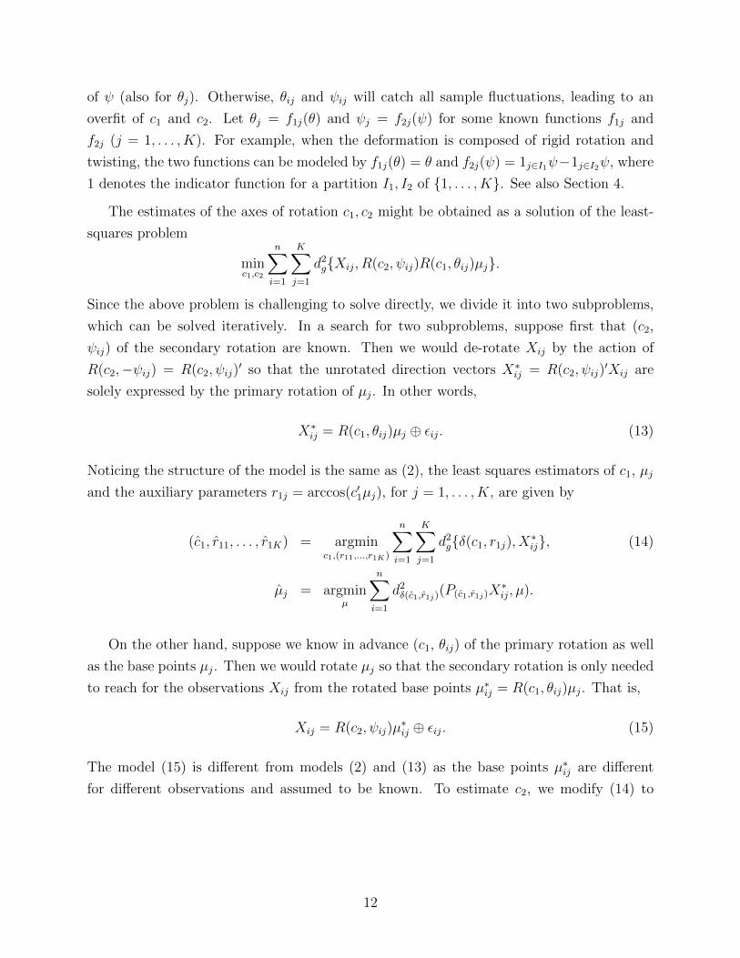
of ψ (also for θj). Otherwise, θij and ψij will catch all sample fluctuations, leading to an

overfit of c1 and c2. Let θj = f1j(θ) and ψj = f2j(ψ) for some known functions f1j and

f2j (j = 1, . . . , K). For example, when the deformation is composed of rigid rotation and

twisting, the two functions can be modeled by f1j(θ) = θ and f2j(ψ) = 1j∈I1ψ−1j∈I2ψ, where

1 denotes the indicator function for a partition I1, I2 of {1, . . . , K}. See also Section 4.

The estimates of the axes of rotation c1, c2 might be obtained as a solution of the least-

squares problem

minc1,c2

n∑i=1

K∑j=1

d2g{Xij, R(c2, ψij)R(c1, θij)µj}.

Since the above problem is challenging to solve directly, we divide it into two subproblems,

which can be solved iteratively. In a search for two subproblems, suppose first that (c2,

ψij) of the secondary rotation are known. Then we would de-rotate Xij by the action of

R(c2,−ψij) = R(c2, ψij)′ so that the unrotated direction vectors X∗ij = R(c2, ψij)

′Xij are

solely expressed by the primary rotation of µj. In other words,

X∗ij = R(c1, θij)µj ⊕ εij. (13)

Noticing the structure of the model is the same as (2), the least squares estimators of c1, µj

and the auxiliary parameters r1j = arccos(c′1µj), for j = 1, . . . , K, are given by

(c1, r11, . . . , r1K) = argminc1,(r11,...,r1K)

n∑i=1

K∑j=1

d2g{δ(c1, r1j), X∗ij}, (14)

µj = argminµ

n∑i=1

d2δ(c1,r1j)(P(c1,r1j)X∗ij, µ).

On the other hand, suppose we know in advance (c1, θij) of the primary rotation as well

as the base points µj. Then we would rotate µj so that the secondary rotation is only needed

to reach for the observations Xij from the rotated base points µ∗ij = R(c1, θij)µj. That is,

Xij = R(c2, ψij)µ∗ij ⊕ εij. (15)

The model (15) is different from models (2) and (13) as the base points µ∗ij are different

for different observations and assumed to be known. To estimate c2, we modify (14) to

12

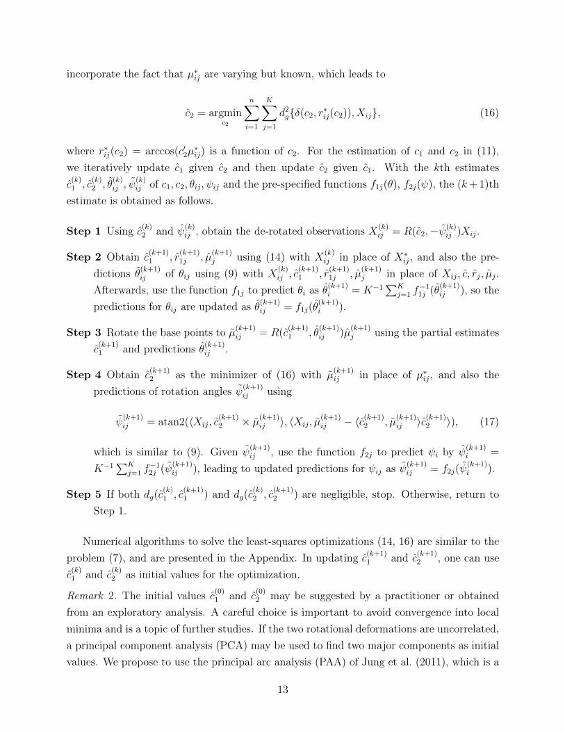
incorporate the fact that µ∗ij are varying but known, which leads to

c2 = argminc2

n∑i=1

K∑j=1

d2g{δ(c2, r∗ij(c2)), Xij}, (16)

where r∗ij(c2) = arccos(c′2µ∗ij) is a function of c2. For the estimation of c1 and c2 in (11),

we iteratively update c1 given c2 and then update c2 given c1. With the kth estimates

c(k)1 , c

(k)2 , θ

(k)ij , ψ

(k)ij of c1, c2, θij, ψij and the pre-specified functions f1j(θ), f2j(ψ), the (k+ 1)th

estimate is obtained as follows.

Step 1 Using c(k)2 and ψ

(k)ij , obtain the de-rotated observations X

(k)ij = R(c2,−ψ(k)

ij )Xij.

Step 2 Obtain c(k+1)1 , r

(k+1)1j , µ

(k+1)j using (14) with X

(k)ij in place of X∗ij, and also the pre-

dictions θ(k+1)ij of θij using (9) with X

(k)ij , c

(k+1)1 , r

(k+1)1j , µ

(k+1)j in place of Xij, c, rj, µj.

Afterwards, use the function f1j to predict θi as θ(k+1)i = K−1

∑Kj=1 f

−11j (θ

(k+1)ij ), so the

predictions for θij are updated as θ(k+1)ij = f1j(θ

(k+1)i ).

Step 3 Rotate the base points to µ(k+1)ij = R(c

(k+1)1 , θ

(k+1)ij )µ

(k+1)j using the partial estimates

c(k+1)1 and predictions θ

(k+1)ij .

Step 4 Obtain c(k+1)2 as the minimizer of (16) with µ

(k+1)ij in place of µ∗ij, and also the

predictions of rotation angles ψ(k+1)ij using

ψ(k+1)ij = atan2(〈Xij, c

(k+1)2 × µ(k+1)

ij 〉, 〈Xij, µ(k+1)ij − 〈c(k+1)

2 , µ(k+1)ij 〉c(k+1)

2 〉), (17)

which is similar to (9). Given ψ(k+1)ij , use the function f2j to predict ψi by ψ

(k+1)i =

K−1∑K

j=1 f−12j (ψ

(k+1)ij ), leading to updated predictions for ψij as ψ

(k+1)ij = f2j(ψ

(k+1)i ).

Step 5 If both dg(c(k)1 , c

(k+1)1 ) and dg(c

(k)2 , c

(k+1)2 ) are negligible, stop. Otherwise, return to

Step 1.

Numerical algorithms to solve the least-squares optimizations (14, 16) are similar to the

problem (7), and are presented in the Appendix. In updating c(k+1)1 and c

(k+1)2 , one can use

c(k)1 and c

(k)2 as initial values for the optimization.

Remark 2. The initial values c(0)1 and c

(0)2 may be suggested by a practitioner or obtained

from an exploratory analysis. A careful choice is important to avoid convergence into local

minima and is a topic of further studies. If the two rotational deformations are uncorrelated,

a principal component analysis (PCA) may be used to find two major components as initial

values. We propose to use the principal arc analysis (PAA) of Jung et al. (2011), which is a

13

generalized PCA for data lying on (S2)K . Jung et al. (2011) argued that non-linear variation

along small circles is better captured by PAA than by other extensions of PCA including

Fletcher et al. (2004) and Huckemann et al. (2010). PAA is well suited to our problem, since

the Xij are distributed along small circles.

We now discuss how to use PAA to obtain initial values. For Xi = (Xi1, . . . , XiK)′ ∈(S2)K (i = 1, . . . , n), PAA gives the mean µPAA = (µPAA1 , . . . , µPAAK )′ ∈ (S2)K and the

projections Xi(m) = (Xi1(m), . . . , XiK(m))′ ∈ (S2)K onto the mth component, m ∈ {1, . . . ,M}

and M is the minimum of 2K and n− 1. The first two components will be used to provide

initial values. Which component corresponds to which rotational motion depends on the

variance of θ and ψ. If Var(θ) of the primary rotation is assumed to be larger than Var(ψ) of

the secondary rotation, then the first component will provide an initial value for the primary

rotation. In such a case, the solutions of (7) and (9) with Xij(1) in place of Xij are used as

the initial values of c(0)1 , θ

(0)ij . Likewise, Xij(2) are used to evaluate c

(0)2 , ψ

(0)ij . On the other

hand, if Var(θ) < Var(ψ), then Xij(1) is used for c(0)2 , and Xij(2) for c

(0)1 .

Remark 3. In contrast to single rotational deformations the function fj affects the estimation

of the rotation axes by the iterative back-and-forward rotation between two deformations

which depend on the angle predictions. The order of the hierarchical deformation is specified

by the primary and secondary information as well as by the functions f1j, f2j. Simulation

studies, reported in Section 4 of the Supplementary Material, discuss the misspecification of

fj and a misspecified deformation order.

4 Numerical studies

In this section, we turn to the numerical performance of the proposed estimators. As our

modeling approach is novel, there is no competing method to compare with. We study

performance over several different rotational deformation situations.

Two different objects are studied. The first object (body 1), illustrated in Fig. 2, consists

of K = 4 directions, while the second object (body 2) contains K = 8 direction vectors. The

von Mises–Fisher distribution (Mardia and Jupp, 2000, p. 36) with concentration parameter

κ, denoted as vMF(κ), is used for the distribution of errors. Three models (indexed by

equation number) are considered for each object:

• Model (2)–Rigid rotation: c = (1, 0, 0)′, θ ∼ N(0, σ2θ) and σθ = π/12 ≈ 15◦.

• Model (10)–Twisting : c = (0, 1, 0)′, θj = fj(θ) = 1j∈I1θ − 1j∈I2θ, where θ ∼ N(0, σ2θ),

14

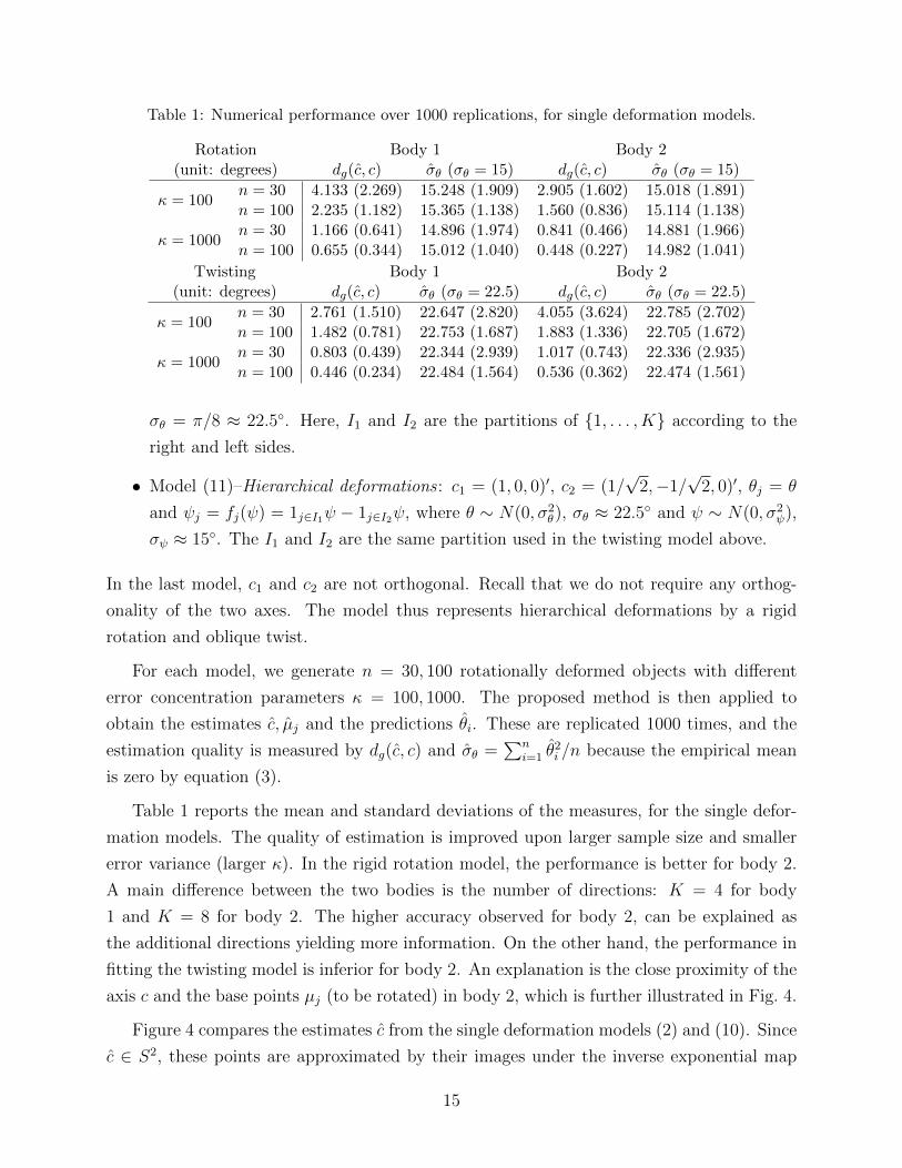
Table 1: Numerical performance over 1000 replications, for single deformation models.

Rotation Body 1 Body 2(unit: degrees) dg(c, c) σθ (σθ = 15) dg(c, c) σθ (σθ = 15)

κ = 100n = 30 4.133 (2.269) 15.248 (1.909) 2.905 (1.602) 15.018 (1.891)n = 100 2.235 (1.182) 15.365 (1.138) 1.560 (0.836) 15.114 (1.138)

κ = 1000n = 30 1.166 (0.641) 14.896 (1.974) 0.841 (0.466) 14.881 (1.966)n = 100 0.655 (0.344) 15.012 (1.040) 0.448 (0.227) 14.982 (1.041)

Twisting Body 1 Body 2(unit: degrees) dg(c, c) σθ (σθ = 22.5) dg(c, c) σθ (σθ = 22.5)

κ = 100n = 30 2.761 (1.510) 22.647 (2.820) 4.055 (3.624) 22.785 (2.702)n = 100 1.482 (0.781) 22.753 (1.687) 1.883 (1.336) 22.705 (1.672)

κ = 1000n = 30 0.803 (0.439) 22.344 (2.939) 1.017 (0.743) 22.336 (2.935)n = 100 0.446 (0.234) 22.484 (1.564) 0.536 (0.362) 22.474 (1.561)

σθ = π/8 ≈ 22.5◦. Here, I1 and I2 are the partitions of {1, . . . , K} according to the

right and left sides.

• Model (11)–Hierarchical deformations : c1 = (1, 0, 0)′, c2 = (1/√

2,−1/√

2, 0)′, θj = θ

and ψj = fj(ψ) = 1j∈I1ψ − 1j∈I2ψ, where θ ∼ N(0, σ2θ), σθ ≈ 22.5◦ and ψ ∼ N(0, σ2

ψ),

σψ ≈ 15◦. The I1 and I2 are the same partition used in the twisting model above.

In the last model, c1 and c2 are not orthogonal. Recall that we do not require any orthog-

onality of the two axes. The model thus represents hierarchical deformations by a rigid

rotation and oblique twist.

For each model, we generate n = 30, 100 rotationally deformed objects with different

error concentration parameters κ = 100, 1000. The proposed method is then applied to

obtain the estimates c, µj and the predictions θi. These are replicated 1000 times, and the

estimation quality is measured by dg(c, c) and σθ =∑n

i=1 θ2i /n because the empirical mean

is zero by equation (3).

Table 1 reports the mean and standard deviations of the measures, for the single defor-

mation models. The quality of estimation is improved upon larger sample size and smaller

error variance (larger κ). In the rigid rotation model, the performance is better for body 2.

A main difference between the two bodies is the number of directions: K = 4 for body

1 and K = 8 for body 2. The higher accuracy observed for body 2, can be explained as

the additional directions yielding more information. On the other hand, the performance in

fitting the twisting model is inferior for body 2. An explanation is the close proximity of the

axis c and the base points µj (to be rotated) in body 2, which is further illustrated in Fig. 4.

Figure 4 compares the estimates c from the single deformation models (2) and (10). Since

c ∈ S2, these points are approximated by their images under the inverse exponential map

15

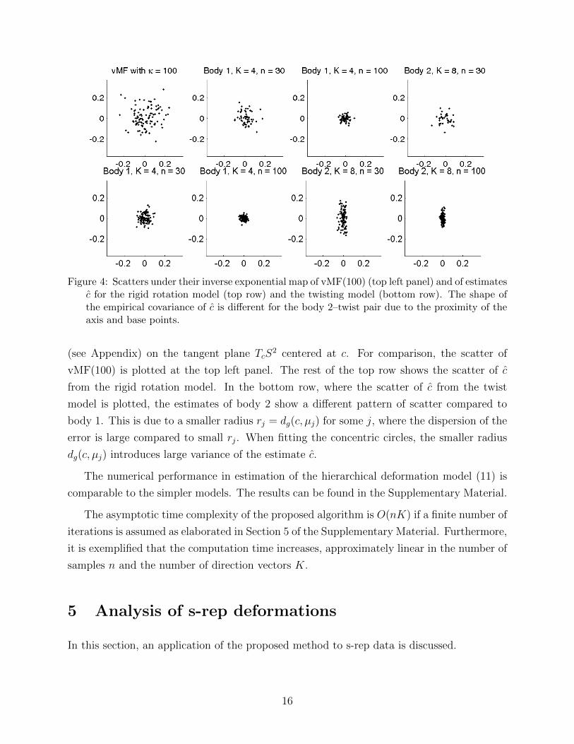
Figure 4: Scatters under their inverse exponential map of vMF(100) (top left panel) and of estimatesc for the rigid rotation model (top row) and the twisting model (bottom row). The shape ofthe empirical covariance of c is different for the body 2–twist pair due to the proximity of theaxis and base points.

(see Appendix) on the tangent plane TcS2 centered at c. For comparison, the scatter of

vMF(100) is plotted at the top left panel. The rest of the top row shows the scatter of c

from the rigid rotation model. In the bottom row, where the scatter of c from the twist

model is plotted, the estimates of body 2 show a different pattern of scatter compared to

body 1. This is due to a smaller radius rj = dg(c, µj) for some j, where the dispersion of the

error is large compared to small rj. When fitting the concentric circles, the smaller radius

dg(c, µj) introduces large variance of the estimate c.

The numerical performance in estimation of the hierarchical deformation model (11) is

comparable to the simpler models. The results can be found in the Supplementary Material.

The asymptotic time complexity of the proposed algorithm is O(nK) if a finite number of

iterations is assumed as elaborated in Section 5 of the Supplementary Material. Furthermore,

it is exemplified that the computation time increases, approximately linear in the number of

samples n and the number of direction vectors K.

5 Analysis of s-rep deformations

In this section, an application of the proposed method to s-rep data is discussed.

16

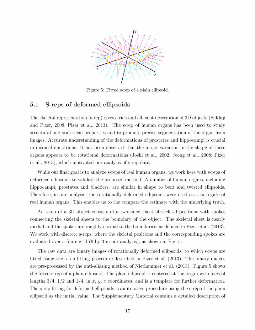
Figure 5: Fitted s-rep of a plain ellipsoid.

5.1 S-reps of deformed ellipsoids

The skeletal representation (s-rep) gives a rich and efficient description of 3D objects (Siddiqi

and Pizer, 2008; Pizer et al., 2013). The s-rep of human organs has been used to study

structural and statistical properties and to promote precise segmentation of the organ from

images. Accurate understanding of the deformations of prostates and hippocampi is crucial

in medical operations. It has been observed that the major variation in the shape of these

organs appears to be rotational deformations (Joshi et al., 2002; Jeong et al., 2008; Pizer

et al., 2013), which motivated our analysis of s-rep data.

While our final goal is to analyze s-reps of real human organs, we work here with s-reps of

deformed ellipsoids to validate the proposed method. A number of human organs, including

hippocampi, prostates and bladders, are similar in shape to bent and twisted ellipsoids.

Therefore, in our analysis, the rotationally deformed ellipsoids were used as a surrogate of

real human organs. This enables us to the compare the estimate with the underlying truth.

An s-rep of a 3D object consists of a two-sided sheet of skeletal positions with spokes

connecting the skeletal sheets to the boundary of the object. The skeletal sheet is nearly

medial and the spokes are roughly normal to the boundaries, as defined in Pizer et al. (2013).

We work with discrete s-reps, where the skeletal positions and the corresponding spokes are

evaluated over a finite grid (9 by 3 in our analysis), as shown in Fig. 5.

The raw data are binary images of rotationally deformed ellipsoids, to which s-reps are

fitted using the s-rep fitting procedure described in Pizer et al. (2013). The binary images

are pre-processed by the anti-aliasing method of Niethammer et al. (2013). Figure 5 shows

the fitted s-rep of a plain ellipsoid. The plain ellipsoid is centered at the origin with axes of

lengths 3/4, 1/2 and 1/4, in x, y, z coordinates, and is a template for further deformation.

The s-rep fitting for deformed ellipsoids is an iterative procedure using the s-rep of the plain

ellipsoid as the initial value. The Supplementary Material contains a detailed description of

17

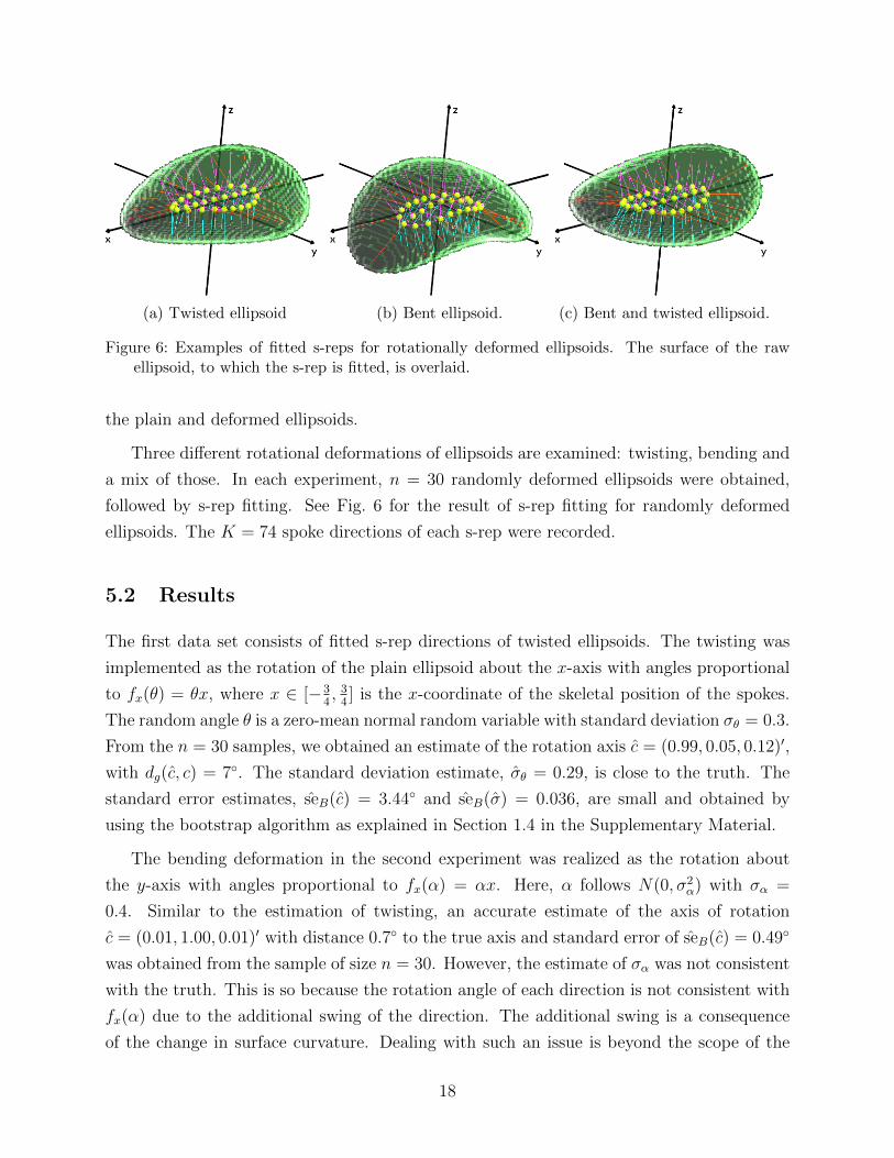
(a) Twisted ellipsoid (b) Bent ellipsoid. (c) Bent and twisted ellipsoid.

Figure 6: Examples of fitted s-reps for rotationally deformed ellipsoids. The surface of the rawellipsoid, to which the s-rep is fitted, is overlaid.

the plain and deformed ellipsoids.

Three different rotational deformations of ellipsoids are examined: twisting, bending and

a mix of those. In each experiment, n = 30 randomly deformed ellipsoids were obtained,

followed by s-rep fitting. See Fig. 6 for the result of s-rep fitting for randomly deformed

ellipsoids. The K = 74 spoke directions of each s-rep were recorded.

5.2 Results

The first data set consists of fitted s-rep directions of twisted ellipsoids. The twisting was

implemented as the rotation of the plain ellipsoid about the x-axis with angles proportional

to fx(θ) = θx, where x ∈ [−34, 34] is the x-coordinate of the skeletal position of the spokes.

The random angle θ is a zero-mean normal random variable with standard deviation σθ = 0.3.

From the n = 30 samples, we obtained an estimate of the rotation axis c = (0.99, 0.05, 0.12)′,

with dg(c, c) = 7◦. The standard deviation estimate, σθ = 0.29, is close to the truth. The

standard error estimates, seB(c) = 3.44◦ and seB(σ) = 0.036, are small and obtained by

using the bootstrap algorithm as explained in Section 1.4 in the Supplementary Material.

The bending deformation in the second experiment was realized as the rotation about

the y-axis with angles proportional to fx(α) = αx. Here, α follows N(0, σ2α) with σα =

0.4. Similar to the estimation of twisting, an accurate estimate of the axis of rotation

c = (0.01, 1.00, 0.01)′ with distance 0.7◦ to the true axis and standard error of seB(c) = 0.49◦

was obtained from the sample of size n = 30. However, the estimate of σα was not consistent

with the truth. This is so because the rotation angle of each direction is not consistent with

fx(α) due to the additional swing of the direction. The additional swing is a consequence

of the change in surface curvature. Dealing with such an issue is beyond the scope of the

18

current paper; it is discussed further in the Supplementary Material.

Finally, we report the results for bent and twisted ellipsoids. The raw ellipsoids were

sequentially deformed by bending about the y-axis, then twisting about the x-axis. The

initial values chosen by the data-driven method (see Remark 2 in Section 3) are c01 =

(−0.13,−0.99,−0.00)′ and c02 = (−0.07,−0.99, 0.02)′, which are almost the same. A uni-

formly randomly chosen initial value for c2 was used instead. In particular, a uniform ran-

dom direction c02 was used, provided that c02 is at least 11 degrees away from c01. With this

alternative initial value, the iterative estimation leads to estimates c1 = (0.01,−1,−0.00)′

and c2 = (−0.99 − 0.05, 0.00)′, both of which are close to their corresponding population

counterparts. The estimated standard error seB(c1) = 3.34◦ of the first rotation axis is small

in contrast to the second rotation axis with seB(c2) = 27.50◦. This indicates that a precise

estimation of the rotation angle is critical for hierarchical deformations. In contrast to single

deformations the rotation angles affect the estimation of the rotation axes (cf. Remark 3

in Section 3). Thus, the large standard error is a result of the inaccurate estimate of the

rotation angle α in case of bending as discussed in the previous paragraph.

As we have pointed out in the introduction, the ellipsoid considered here can be under-

stood as a template for many real human organs. The accurate estimation of the parameters

of rotational deformations of ellipsoids indicates the potential of this type of analysis of de-

formed objects in real 3D images obtained from, e.g., magnetic resonance imaging. Further

experiments cover surface point distribution models and a more general deformation; they

are discussed in the Supplementary Material.

6 Application to knee motion during gait

In order to further support the validity of the proposed estimation procedure, this section

presents findings from experimentally collected biomechanical data as a part of a larger

project (Pierrynowski et al., 2010).

The estimation of two rotation axes of the knee joint is a well-studied problem in biome-

chanics (e.g., Ball and Greiner (2012)). The two estimated rotation axes model the primary

and secondary rotation axes of the upper and lower leg relative to each other. The dominant

rotation axis defines the flexion-extension motion at the knee. This axis is approximately

directed right-to-left (lateral-to-medial). The secondary rotation axis defines the internal-

external motion of the lower leg relative to the upper leg. This axis is approximately directed

down-to-up (distal-to-proximal) along the long axis of the tibia (ankle-to-knee joint centers).

19

The motion of 25 markers placed on the right lower extremity of one healthy male volun-

teer was collected following informed consent. To provide measures of the motion of the bones

within the lower leg and thigh the volunteer consented to have two 6 mm pins surgically in-

serted into his femur and tibia using local anesthesia. The methodological concerns cited by

Ramsey et al. (2003) were followed to guide pin placement. The insertion sites were selected

to minimize neuro-muscular effects that could influence natural knee motion. Self-report by

the volunteer stated that the pins were not painful and did not influence his walking pattern.

Three and four markers were then attached to these rigid pins which allowed us to measure

the true motion of the hidden femur and tibia bones. Additional markers were also placed

on the surface of the thigh (10 skin markers) and lower leg (8 skin markers). In each of the

four segments (femur, tibia, thigh, lower leg) one marker was chosen as a basis point and

directions were derived between the basis point and the remaining markers of that segment,

described in detail in Section 6 in the Supplementary Material. The coordinate system for

this experiment was defined when the volunteer stood at attention and faced forwards. The

XYZ axes were in the directions Forward, Inward, Upward (FIU). During movement, the leg

XYZ axes relative to the thigh XYZ axes were used for the analysis.

The volunteer walked at 2.5 mph on a motor driven treadmill. After a familiarization

time period, the motion of the markers were collected for approximately 20 seconds at 50

Hz. Within this data collection period, 16 complete gait cycles were identified. A gait cycle

is defined from right foot contact with the floor to the next right foot contact. In total 976

time points were used within the following analyses.

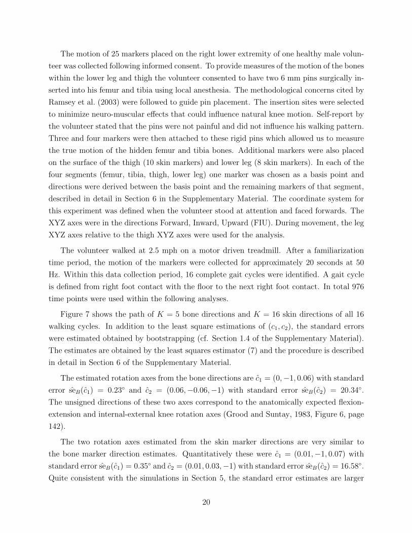
Figure 7 shows the path of K = 5 bone directions and K = 16 skin directions of all 16

walking cycles. In addition to the least square estimations of (c1, c2), the standard errors

were estimated obtained by bootstrapping (cf. Section 1.4 of the Supplementary Material).

The estimates are obtained by the least squares estimator (7) and the procedure is described

in detail in Section 6 of the Supplementary Material.

The estimated rotation axes from the bone directions are c1 = (0,−1, 0.06) with standard

error seB(c1) = 0.23◦ and c2 = (0.06,−0.06,−1) with standard error seB(c2) = 20.34◦.

The unsigned directions of these two axes correspond to the anatomically expected flexion-

extension and internal-external knee rotation axes (Grood and Suntay, 1983, Figure 6, page

142).

The two rotation axes estimated from the skin marker directions are very similar to

the bone marker direction estimates. Quantitatively these were c1 = (0.01,−1, 0.07) with

standard error seB(c1) = 0.35◦ and c2 = (0.01, 0.03,−1) with standard error seB(c2) = 16.58◦.

Quite consistent with the simulations in Section 5, the standard error estimates are larger

20

(a) bone (b) skin

Figure 7: Estimation of first (flexion-extension) and second (internal-external) rotation axes ofthe knee from bone and skin marker directions on the upper (femur; thigh) and lower (tibia;lower leg) extremity. In addition, the path of each marker direction is depicted. (a) Estimatedrotation axes of directions derived from bone markers. (b) Estimated rotation axes of directionsderived from skin markers.

for the second axis. In both cases (bone and skin data), the higher standard error of the

second rotation axis is due to the small range of rotation angles about this axis. The larger

standard error of the second axis for the bone data is deemed to be a result of the small

number of observed directions. Estimation results of the rotation angles can be found in

the Supplementary Material. Future work lies in the improved estimation based on a more

careful time modeling of knee motions such as that proposed by Rivest (2001) who examined

elbow motion.

7 Discussion

The paper proposes a novel nonparametric method to estimate rotational deformations from

directional data. For the simple, single rotational deformation, the estimation procedure

does not depend on the latent variable θj. In addition, the paper proposed an estimation

procedure for hierarchical deformations, which depends on the order and the specification of

functions f1j, f2j. An important future research is the improved prediction of the rotation

angles θj and ψj, in particular for hierarchical rotations as introduced in Section 3. This

includes the classification of directions into carefully chosen partitions I1 and I2 as well as the

development of methods to predict fj from the data as noted in Remarks 1 and 3. In order

to extend the estimation method to more than two rotational deformations, characterization

of geometry related to composition of hierarchical deformations is essential. A first step in

21

decreasing the relevance of the order of deformations would be the implementation of an

expectation-maximization (EM) based optimization procedure.

Appendix

Proof of Lemma 1

Let Aj = {vj ∈ δη(c, rj)}, where δη(c, r) = {x ∈ S2 : dg(δ(c, r), x) < η}. For R = R(c, θ),

P (Aj) = P [dg{Rµj ⊕ εj, δ(c, rj)} < η] = P [dg{RT (Rµj ⊕ εj), RT δ(c, rj)} < η]

= P [dg{µj ⊕ ε, δ(c, rj)} < η] ≥ P [dg(µj ⊕ ε, µj) < η] ≥ 1− Var(ε)/η2,

where µj ⊕ ε has the same distribution as RT (Rµj ⊕ εj) because of the spherical symmetry.

A Markov inequality is used. Since the Ajs are independent, P (⋂Kj=1Aj) =

∏Kj=1 P (Aj) ≥

{1− Var(ε)/η2}K .

Numerical Algorithms for (7), (14), and (16)

The optimization problems (7) and (14) are identical and can be understood as fitting con-

centric circles on the unit sphere. The problem (16) is a more general nonlinear least squares

problem, which however can be solved in a similar manner to the former two problems. We

propose a variant of the doubly iterative algorithm used in fitting small circles in Sm (Jung

et al., 2011, 2012).

We first introduce some notation. For m ≥ 2, the tangent space at c ∈ Sm is denoted

by TcSm, which can be parametrized by Rm. Let c = em+1 without loss of generality. The

exponential map Expc : Rm → Sm is defined for v1 ∈ Rm by

Expc(v1) =

(v1‖v1‖

sin ‖v1‖, cos ‖v1‖),

with a convention of Expc(0) = c. The exponential map has an inverse, called the log map,

and is denoted by Logc : Sm → TcSm.

For problems (7) and (14), the following iterative algorithm can be used. The algorithm

finds a suitable point of tangency c0, which is also the center of the fitted concentric circles.

Given the candidate c0, the data xij are mapped to the tangent space Tc0S2 by the Log map.

Let x†ij = Logc0(xij). Since the Log map preserves distance, we have arccos(c′0xij) = ‖x†ij‖.

22

Then we solve a non-linear least-squares problem

minc†,rj

n∑i=1

K∑j=1

(‖x†ij − c†‖ − rj)2. (18)

Since the optimization problem (18) does not have any constraint, it can be numerically

solved by, e.g., the Levenberg–Marquardt algorithm (Scales, 1985). The solution c† is then

mapped to S2 by the exponential map at c and becomes c1. This procedure is repeated until

c converges.

The optimization problem (16) can be solved in a similar way. We use the fact that

d2g(δ(c, r∗(c)), x) = (arccos(c′x)− arccos(c′µ∗))2 = (‖Logcx‖ − ‖Logcµ

∗‖)2. Thus for fixed c,

d2g(δ(c, r∗(c)), x) ≥ miny(‖Logcx − y‖ − ‖Logcµ

∗ − y‖)2. The minimizer y leads to a better

candidate for c through the exponential map. The algorithm to solve (16) follows the same

lines as the algorithm to solve (7), except instead of (18) we minimize

minc†

n∑i=1

K∑j=1

(‖Logcx− c†‖ − ‖Logcµ− c†‖)2.

Supplementary Materials

Additional discussions and data analyses: Article containing i.) additional data anal-

ysis results, ii.) simulation results for the hierarchical deformation model described in

Section 4, iii.) further discussion of the model bias, brought up in Section 2.1, iv.)

study of the estimator behaviour using misspecified parameters, v.) a computational

complexity study of the algorithm and vi.) the estimation procedure for knee motion

analysis during gait as discussed in Section 6. (SupplementaryMaterialSJ.pdf)

Matlab code: A set of Matlab code for application of the proposed method. The code also

contains all datasets used as examples in the article. (estRotDeformation.zip)

Acknowledgments

The work of J. Schulz was funded by Norwegian Research Council through eVita program

grant no 176872/V30. His research was performed as part of Tromsø Telemedicine Lab-

oratory, funded by the Norwegian Research Council 2007-2014, grant no 174934. S. Jung

was partially supported by NSF grant DMS-1307178. S. Huckemann gratefully acknowledges

support from the Niedersachsen Vorab and DFG HU 1575/4-1. The work of M. Pierrynowski

23

work was supported by a travel grant from McMaster University. The authors would like

to thank Chong Shao and Wenqi Zhang for their help in generating the ellipsoid data, and

Jared Vicory for advice on running Pablo.

References

Altmann, S. L. (2005), Rotations, Quaternions, and Double Groups, Dover books on math-

ematics, Dover Publications.

Ball, K. A. and Greiner, T. M. (2012), “A Procedure to Refine Joint Kinematic Assessments:

Functional Alignment,” Computer Methods in Biomechanics and Biomedical Engineering,

15, 487–500.

Chang, T. (1986), “Spherical Regression,” The Annals of Statistics, 14, 907–924.

— (1988), “Estimating the Relative Rotation of Two Tectonic Plates from Boundary Cross-

ings,” Journal of the American Statistical Association, 83, 1178–1183.

— (1989), “Spherical Regression with Errors in Variables,” The Annals of Statistics, 17,

293–306.

Chang, T. and Rivest, L.-P. (2001), “M-Estimation for Location and Regression Parameters

in Group Models: A Case Study using Stiefel Manifolds,” The Annals of Statistics, 29,

784–814.

Chapman, G. R., Chen, G., and Kim, P. T. (1995), “Assessing Geometric Integrity Through

Spherical Regression Techniques,” Statistica Sinica, 5, 173–220.

Cootes, T. F., Taylor, C., Cooper, D., and Graham, J. (1992), “Training Models of Shape

from Sets of Examples,” in Proc. British Machine Vision Conference, eds. Hogg, D. and

Boyle, R., Berlin. Springer-Verlag, pp. 9–18.

Dryden, I. L. and Mardia, K. V. (1998), Statistical Shape Analysis, Chichester: Wiley.

Fisher, N. I., Lewis, T., and Embleton, B. J. J. (1993), Statistical Analysis of Spherical Data,

Cambridge: Cambridge University Press.

Fletcher, P., Lu, C., and Joshi, S. (2003), “Statistics of Shape via Principal Geodesic Analysis

on Lie Groups,” in Computer Vision and Pattern Recognition, 2003. Proceedings. 2003

IEEE Computer Society Conference on, vol. 1, pp. I–95–I–101 vol.1.

24

Fletcher, P. T., Lu, C., Pizer, S. M., and Joshi, S. (2004), “Principal Geodesic Analysis for

the Study of Nonlinear Statistics of Shape,” IEEE Transactions on Medical Imaging, 23,

995–1005.

Frechet, M. (1948), “Les Elements Aleatoires de Nature Quelconque dans un Espace Dis-

tancie,” Annales de l’Institut Henri Poincare, 10, 215–310.

Gamage, S. S. and Lasenby, J. (2002), “New Least Squares Solutions for Estimating the

Average Centre of Rotation and the Axis of Rotation,” Journal of Biomechanics, 35,

87–93.

Goodall, C. R. (1991), “Procrustes Methods in the Statistical Analysis of Shape (with dis-

cussion),” Journal of the Royal Statistical Society: Series B, 53, 285–339.

Gray, J. J. (1980), “Olinde Rodrigues’ Paper of 1840 on Transformation Groups,” Archive

for History of Exact Sciences, 21, 375–385.

Grood, E. and Suntay, W. (1983), “A joint coordinate system for the clinical description of

three-dimensional motions: Application to the knee,” Journal of Biomechanical Engineer-

ing, 105, 136–144.

Halvorsen, K., Lesser, M., and Lundberg, A. (1999), “A new Method for Estimating the

Axis of Rotation and the Center of Rotation,” Journal of Biomechanics, 32, 1221–1227.

Hanna, M. S. and Chang, T. (2000), “Fitting Smooth Histories to Rotation Data,” Journal

of Multivariate Analysis, 75, 47–61.

Huckemann, S. (2011a), “Inference on 3D Procrusted Means: Tree Bole Growth, Rank

Deficient Diffusion Tensors and Perturbation Models,” Scandinavian Journal of Statistics,

38, 424–446.

— (2011b), “Intrinsic Inference on the Mean Geodesic of Planar Shapes and Tree Discrimi-

nation by Leaf Growth,” Annals of Statistics, 39, 1098–1124.

— (2012), “On the Meaning of Mean Shape: Manifold Stability, Locus and the Two Sample

Test,” Annals of the Institute of Statistical Mathematics, 64, 1227–1259.

Huckemann, S., Hotz, T., and Munk, A. (2010), “Intrinsic Shape Analysis: Geodesic PCA

for Riemannian Manifolds modulo Isometric Lie Group Actions,” Statistica Sinica, 20,

1–58.

25

Jeong, J.-Y., Stough, J. V., Marron, J. S., and Pizer, S. M. (2008), “Conditional-Mean

Initialization Using Neighboring Objects in Deformable Model Segmentation,” in SPIE

Medical Imaging.

Joshi, S., Pizer, S. M., Fletcher, P., Yushkevich, P., Thall, A., and Marron, J. S. (2002),

“Multiscale Deformable Model Segmentation and Statistical Shape Analysis Using Medial

Descriptions,” IEEE Transactions on Medical Imaging, 21, 538–550.

Jung, S., Dryden, I. L., and Marron, J. S. (2012), “Analysis of Principal Nested Spheres,”

Biometrika, 99, 551–568.

Jung, S., Foskey, M., and Marron, J. S. (2011), “Principal Arc Analysis on Direct Product

Manifolds,” Annals of Applied Statistics, 5, 578–603.

Karcher, H. (1977), “Riemannian Center of Mass and Mollifier Smoothing,” Communications

on Pure and Applied Mathematics, 30, 509–541.

Kent, J. T. and Mardia, K. V. (1997), “Consistency of Procrustes Estimators,” Journal of

the Royal Statistical Society: Series B, 59, 281–290.

Kurtek, S., Ding, Z., Klassen, E., and Srivastava, A. (2011), “Parameterization-Invariant

Shape Statistics and Probabilistic Classification of Anatomical Surfaces,” in Information

Processing in Medical Imaging, vol. 22, pp. 147–158.

Le, H. (1998), “On the Consistency of Procrustean Mean Shapes,” Advances in Applied

Probability, 30, 53–63.

— (2001), “Locating Frechet Means with Application to Shape Spaces,” Advances in Applied

Probability, 33, 324–338.

Mardia, K. V. and Gadsden, R. J. (1977), “A Circle of Best Fit for Spherical Data and Areas

of Vulcanism,” Journal of the Royal Statistical Society: Series C, 26, 238–245.

Mardia, K. V. and Jupp, P. E. (2000), Directional Statistics, Chichester: Wiley.

Moakher, M. (2002), “Means and Averaging in the Group of Rotations,” SIAM Journal on

Matrix Analysis and Applications, 24, 1–16 (electronic).

Niethammer, M., Juttukonda, M. R., Pizer, S. M., and Saboo, R. R. (2013), “Anti-Aliasing

Slice-Segmented Medical Images via Laplacian of Curvature Flow,” In preparation.

Oualkacha, K. and Rivest, L.-P. (2012), “On the Estimation of an Average Rigid Body

Motion,” Biometrika, 99, 585–598.

26

Pennec, X. (2008), “Statistical Computing on Manifolds: from Riemannian Geometry to

Computational Anatomy,” Emerging Trends in Visual Computing, 5416, 347–386.

Pierrynowski, M., Costigan, P., Maly, M., and Kim, P. (2010), “Patients with Osteoarthritic

Knees Have Shorter Orientation and Tangent Indicatrices During Gait,” Clinical Biome-

chanics, 25, 237–241.

Pizer, S. M., Jung, S., Goswami, D., Zhao, X., Chaudhuri, R., Damon, J. N., Huckemann,

S., and Marron, J. S. (2013), “Nested Sphere Statistics of Skeletal Models,” in Innovations

for Shape Analysis: Models and Algorithms, eds. Breuß, M., Bruckstein, A., and Maragos,

P., Springer, Lecture Notes in Computer Science, pp. 93–115.

Ramsey, D. K., Wretenberg, P. F., Benoit, D. L., Lamontagne, M., and Nemeth, G. (2003),

“Methodological concerns using intra-cortical pins to measure tibiofemoral kinematics,”

Knee surgery, sports traumatology, arthroscopy : official journal of the ESSKA, 11, 344–

349.

Rancourt, D., Rivest, L.-P., and Asselin, J. (2000), “Using Orientation Statistics to Inves-

tigate Variations in Human Kinematics,” Journal of the Royal Statistical Society: Series

C, 49, 81–94.

Rivest, L.-P. (1989), “Spherical Regression for Concentrated Fisher-Von Mises Distribu-

tions,” The Annals of Statistics, 17, 307–317.

— (1998), “Some Linear Models for Estimating the Motion of Rigid Bodies with Applications

to Geometric Quality Assurance,” J. Amer. Statist. Assoc., 93, 632–642.

— (1999), “Some Linear Model Techniques for Analyzing Small-Circle Spherical Data,”

Canadian Journal of Statistics, 27, 623–638.

— (2001), “A Directional Model for the Statistical Analysis of Movement in Three Dimen-

sions,” Biometrika, 88, 779–791.

— (2006), “Regression and Correlation for 3 × 3 Rotation Matrices,” Canadian Journal of

Statistics, 34, 1–17.

Rivest, L.-P., Baillargeon, S., and Pierrynowski, M. (2008), “A Directional Model for the

Estimation of the Rotation Axes of the Ankle Joint,” Journal of the American Statistical

Association, 103, 1060–1069.

27

Rohde, G. K., Ribeiro, A. J. S., Dahl, K. N., and Murphy, R. F. (2008), “Deformation-Based

Nuclear Morphometry: Capturing Nuclear Shape Variation in HeLa Cells,” Cytometry A,

73, 341–350.

Scales, L. E. (1985), Introduction to Nonlinear Optimization, New York: Springer-Verlag.

Siddiqi, K. and Pizer, S. (2008), Medial Representations: Mathematics, Algorithms and Ap-

plications, Computational Imaging and Vision, Vol. 37, Dordrecht, Netherlands: Springer,

1st ed.

Teu, K. K. and Kim, W. (2006), “Estimation of the Axis of a Screw Motion from Noisy

Data–A New Method Based on Plucker Lines,” Journal of Biomechanics, 39, 2857–2862.

28