Embed Size (px)
Citation preview

Analysis of Reliability Data Using JMP:
Life Distribution or Recurrence Analysis?
David Trindade, Ph.D.
JMP Discovery Summit, San Diego, CA September 2015
Abstract
In analyzing reliability data from repairable systems, engineers may incorrectly use the
JMP Life Distribution platform to model the times between failures. However, such an
analysis, which disregards the time order of the observations, can lead to invalid
conclusions. The Recurrence Analysis platform in JMP provides appropriate techniques
for modeling reliability data from repairable systems.
This talk will include examples of the improper application of the life distribution approach
to repairable system data and the discovery analysis resulting when the correct
recurrence analysis methodology is applied. The talk will also highlight some limitations of
mean time between failures (MTBF) as a reliability summary statistic and illustrate how
MTBF values reported in the literature can be artificially inflated.
In addition, we’ll suggest some useful enhancements that could be added to the JMP
Recurrence Analysis platform.
Page 2

Objectives
Describe the differences in the analysis of reliability data from non-
repairable and repairable systems.
Illustrate several applications of JMP’s Reliability Analysis platform.
Illustrate some limitations on the use of the summary statistic MTBF as
a measure of reliability.
Show and extend some examples of modeling recurrence data for
prediction purposes.
Suggest some additional, desirable capabilities to the JMP recurrence
analysis reports.

Definition of a Repairable System
A system is repairable if, following a failure at
some time t, it can be restored to satisfactory
operation by any action.

5
Examples of Repairable Systems
Repairable Systems include:
• Automobiles
• TV’s
• Personal Computers
• Network Servers
• Robots
• Automated Manufacturing Equipment
• Airplanes
• Software programs

Examples of Repair Actions
Restoring actions include:
• Replacing a failed component, e.g. circuit board
• Rebooting a computer
• Correcting a software bug
• Adjusting settings
• Swapping of parts
• Automatic switchover to a redundant component
• Restoring electrical power
• Sharp blow with an object (Fonzie approach!)
Common Measures for the Reliability of
Repairable Systems
Age of System at Repair
The total accumulated running hours, days, cycles, miles,
etc. on a system. We’ll use time in hours or days for our analyses.
Times Between Repairs
Called interarrival times.
We’ll assume actual repair times are negligible compared to operating hours. Hence, downtime and availability will be not considered in this discussion.

Reliability of Repairable Systems
Function of many factors
– Basic system design
– Operating conditions
– Environment
– Software robustness
– Type of repairs
– Quality of repairs
– Materials used
– Suppliers
Many factors can vary during system operation.

Fundamental Property of Repairable Systems
Failures occur sequentially in time in systems.
10
For non-repairable components, the usual assumption
made for analysis is that the times to failure are
independent and identically distributed (iid) random
samples from a single population of lifetimes.
For repairable systems, we will show that it is a poor
practice to group together all times between failures for
analysis, disregarding any occurrence order of the data.
Non-Repairable Vs. Repairable Systems

11
For example, in stress testing, because of oven limitations,
a large group of non-repairable units may be separated
into subgroups and each subgroup run one after the other,
with failure times recorded, for a specified time period.
When all runs are done, the times to failure for subgroups
are combined into a single group for a valid analysis.
Are these iid assumptions justified for repairable systems?
Non-Repairable Analysis: Order of Data Acquisition is Irrelevant

12
Case Study Example
Production Equipment:
A new design for a manufacturing system is based on a
single, replaceable component, a circuit board. Upon
system failure, repairs are made by replacing the failed
board with a new, identical board from a stockpile.
Objective of Analysis:
Engineers wanted to model the reliability of the system
based on failure data obtained during the first 1,000 hours
(i.e., 42 days) of operation under accelerated conditions.

13
System Repair History
Repairs (board replacements) were done at system ages
108, 178, 273, 408, 548, 658, 838, and 988 (hours).
A dot plot of repair times is shown below.

14
Case Study Weibull Analysis
The engineers analyzed the data using the time to failure for
each new replacement board, based on the operating hours
between repairs, and treated those times as a group of
independent observations from a single lifetime distribution.
The actual order in which these times occurred (i.e., age of the
system at board replacement) was ignored.
Weibull analysis methods were used for modeling. This common
analysis of times between failures is incorrect and misleading.
15
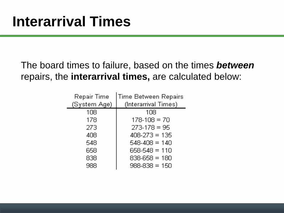
Interarrival Times
The board times to failure, based on the times between
repairs, the interarrival times, are calculated below:

16
JMP Data Table and Life Distribution Analysis
The Life Distribution platform in
JMP [1] is run using Times Between
Failures for Y, Time to Event
Censor = 0 represents a failure
Censor = 1 is a suspension (unit
still operating at test end)
Production Equipment Data Table

17
JMP Life Distribution Analysis: CDF Plot
The Weibull distribution appears to be a good fit to the data.

18
JMP Life Distribution Analysis: Probability Plot
Weibull probability plot shows data points falling close to a straight line.

19
Estimated Weibull Parameters
The Weibull parameter estimates show a characteristic
life a ≈ 136 hours and a shape parameter b ≈ 4.3.
For the Weibull distribution, b > 1.0 indicates an
increasing hazard rate (instantaneous failure rate).
20
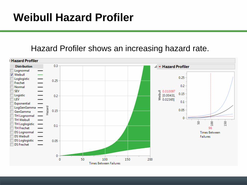
Weibull Hazard Profiler
Hazard Profiler shows an increasing hazard rate.

21
Engineers’ Interpretation of Analysis
Engineers concluded times between repairs were modeled by a Weibull distribution.
The estimated Weibull shape parameter, b>1, indicated an increasing “failure rate.”
The inference was that the equipment had worsening reliability and should be considered for additional repair and maintenance.
Were these conclusions justified or misleading based on the analysis methods applied?
We shall show that this analysis is not appropriate for such data and yields erroneous conclusions.
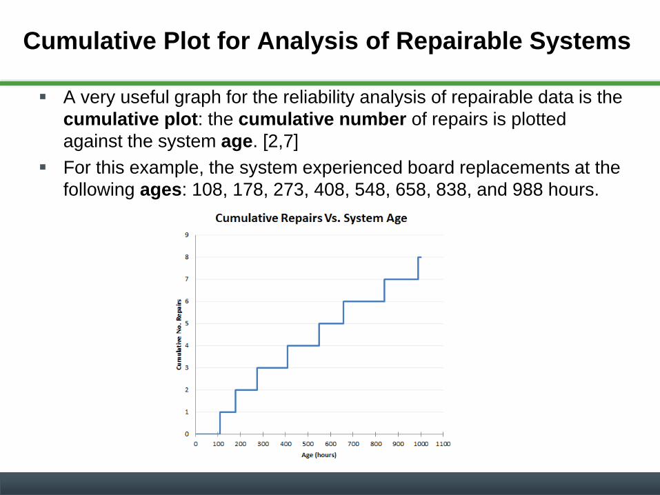
Cumulative Plot for Analysis of Repairable Systems
A very useful graph for the reliability analysis of repairable data is the
cumulative plot: the cumulative number of repairs is plotted
against the system age. [2,7]
For this example, the system experienced board replacements at the
following ages: 108, 178, 273, 408, 548, 658, 838, and 988 hours.
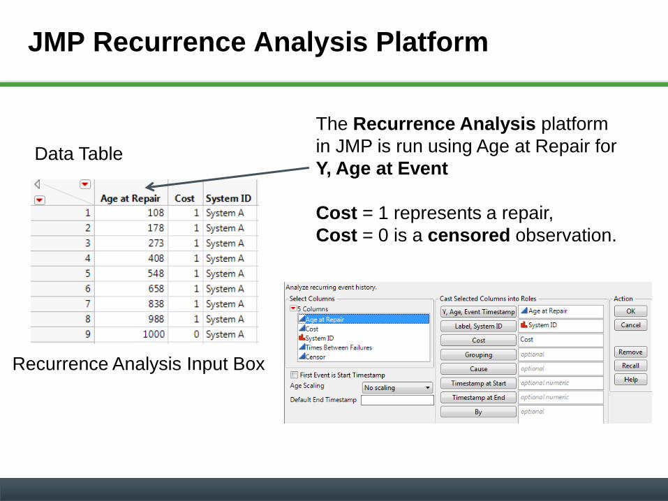
JMP Recurrence Analysis Platform
Data Table
Recurrence Analysis Input Box
The Recurrence Analysis platform
in JMP is run using Age at Repair for
Y, Age at Event
Cost = 1 represents a repair,
Cost = 0 is a censored observation.

JMP shows both an Event Plot
and a Mean Cumulative
Function or MCF Plot. [2,3,4,7]
MCF plot for a single system is
the cumulative plot.
The plot shows no evidence of
system reliability getting
worse with system age.
Let’s consider the sequential
times between repairs.
Cumulative Plot of Number of Repairs Vs. Age

Sequence of Failure Times in Repairable Systems
If the times between successive failures are getting
longer, then the system reliability is improving.
Conversely, if the times between failures are
becoming shorter, the reliability of the system is
degrading.
Thus, the sequence of system failure times can be
very important.
If the times show no trend (relatively stable behavior),
the system may be neither improving or degrading,
which may be suggestive of a constant mean time
between failures (MTBF).

Plot of Times Between Repairs Vs. Age
The plot of the sequential times between repairs versus
the system age at repair shows an increasing trend.
Graph shows times between
repairs increasing.
System reliability is actually
improving!

Results/Implementation
Analysis of the repairable system data using non-
repairable Weibull analysis methods produced a
false conclusion.
Wrong interpretation was caused by the exclusion of
the occurrence order of failures in Weibull analysis.
The correct recurrence analysis showed an
improving trend in the repairable system history.
With the correct analysis, engineers avoided
unneeded expensive, corrective actions and instead
focused on finding the reasons for the improvement.

Analysis of Multiple Repairable Systems
Data may come from many similar systems
possibly subjected to multi-censoring.
Examples:
• Servers installed in the field at different dates
throughout the year will have different ages at a
specified calendar date.
• For autos, vehicles sold on the same date can
have different mileages at the time of analysis.

Reliability Issues for Multiple Systems
Warranty analysis seeks answers to:
• What’s the mean number of repairs by age t?
• What’s the repair rate for all systems at age t?
• What’s the variation in the mean number of repairs at a
given age?
• What’s the expected age to first repair? To kth repair?
• What is the mean repair cost?
• Are costs of repairs increasing or decreasing?
• Are spare parts adequate?
• Are there any location dependent issues?

Methods for Analysis of Multi-System Data
Davis in a 1952 paper [5] analyzed the number of miles
between successive major failures of bus engines by
comparing distributions of interarrival miles to first
failure, between first and second failures, and so on.
He found that the average inter-repair miles to be
decreasing. Early interarrival miles were nearly normal,
but later miles were more exponentially distributed.

31
Davis 1952 Bus Engine Data
Miles to 1st failure
(closer to normal distribution).
Miles between 1st and 2nd failures.
Miles between 2nd and 3rd failures.
Miles between 3rd and 4th failures.
Miles between 4th and 5th failures.
(closer to exponential distribution)

The Folly of Combining Davis Data
It’s clear that the distributions of the miles between
sequential repairs are different.
Had all the data been combined together into one
group and treated as a single population of lifetimes
for analysis, the results would have been incorrect
and misleading.
Neglecting the order of occurrence of the repairs
can lead to invalid conclusions.
Page 32
Limitations of Davis Approach
Method required considerable historical data on many
systems.
No overall predictive models were generated for the
• mean number of repairs versus the bus age in miles
• the age in miles to the kth repair
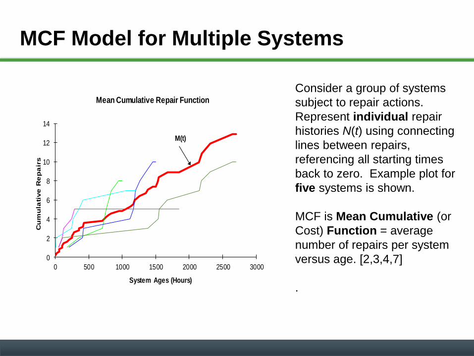
MCF Model for Multiple Systems
Consider a group of systems
subject to repair actions.
Represent individual repair
histories N(t) using connecting
lines between repairs,
referencing all starting times
back to zero. Example plot for
five systems is shown.
MCF is Mean Cumulative (or
Cost) Function = average
number of repairs per system
versus age. [2,3,4,7]
.
0
2
4
6
8
10
12
14
0 500 1000 1500 2000 2500 3000
Cu
mu
lati
ve
Re
pa
irs
System Ages (Hours)
Mean Cumulative Repair Function
M(t)
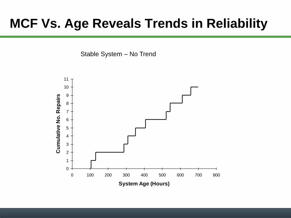
MCF Vs. Age Reveals Trends in Reliability
0
1
2
3
4
5
6
7
8
9
10
11
0 100 200 300 400 500 600 700 800
System Age (Hours)
Cu
mu
lati
ve
No
. R
ep
air
sStable System – No Trend

MCF Vs. Age Reveals Trends in Reliability
0
1
2
3
4
5
6
7
8
9
10
11
0 100 200 300 400 500 600 700 800
System Age (Hours)
Cu
mu
lati
ve
No
. R
ep
air
s
Stable System – No Trend
Here, MTBF is a valid measure. Can draw a straight line through the data.

Caution MTBF – Hides Information
Consider three systems operating for 3000 hours.
System 1 had three failures at 30, 70, 120 hrs and no further failures.
System 2 had three failures at 720, 1580, and 2550 hrs and no further failures.
System 3 had three failures at 2780, 2850, and 2920 hrs and no further failures.
3000 1000 2000 System 1 ***
1000 2000 System 2 * * *
1000 2000 System 3 ***
3000
3000
All systems have the same MTBF = 3000/3 = 1000 hours.
Is the reliability the same for all three systems?

Interpretation of MTBF as Typical Lifetime
MTBF is not the typical lifetime of a
system
Example:
• During the years 1996-1998, the average
annual death rate in the US for children ages
5-14 was 20.8 per 100,000 resident
population.
• The average failure rate is thus 0.02%/yr
• The MTBF is 4,800 years!

Paper Clip Example of Deceptive MTBF
Bend three clips until each breaks: record 6, 5, and 7
breaks to failure
• MTBF = 6
Take a sample of 100 clips and bend each one three
times. Only two break.
• MTBF = 300/2 = 150

MCF Vs. Age Reveals Trends in Reliability
0
1
2
3
4
5
6
7
8
9
10
11
0 100 200 300 400 500 600 700 800
System Age (Hours)
Cu
mu
lati
ve
No
. R
ep
air
s
0
1
2
3
4
5
6
7
8
9
10
11
0 100 200 300 400 500 600 700 800
System Age (Hours)
Cu
mu
lati
ve
No
. R
ep
air
s
Improving System Worsening System
A single MTBF no longer applies as a valid measure.

Example Analysis of Multiple Repairable Systems
We’ll use the JMP sample data file Engine Valve Seat.jmp which
records valve seat replacements in 41 locomotive engines. [6]
Partial table is shown. Each engine has an ID.
Engine 328
TF of Replacements
(Cost = 1):
1st at 326
2nd at 327
3rd at 0
Censor at 14
Engine 328
Ages at
Replacements:
326, 653, 653
Censor at 667

Non-Repairable Component Analysis:
Distributions of TFs of Replaced Valves by Engines
Interarrival TFs and
Censoring Times of
Valves
41 Engine IDs.
Shaded areas are
replacements.
14 Engines had more
than one replacement.
Censor Code:
Censor = 1
Replacement = 0.

Invalid Analysis of Valve Seats as Non-
Repairable Components
We will incorrectly analyze the data
using the time to failure for each
replaced component, as measured by
the time between successive
replacements for each locomotive.

Event Plot and Nonparametric Plot for Times
Between Replacements (Incorrect Analysis)
Arrow Indicates Censored Observation
X Indicates Repair.
Select
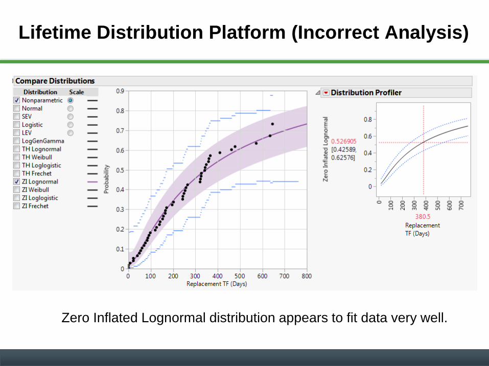
Lifetime Distribution Platform (Incorrect Analysis)
Zero Inflated Lognormal distribution appears to fit data very well.

Hazard Rate Profiler (Incorrect Analysis)
Profiler shows hazard rate increasing early in life, peaking around
100 days, and then continually decreasing thereafter.

Recurrence Analysis: Distributions of System Ages
of Replaced Valves by Engines
Age at Replacement
and Censoring Times
of Valves
41 Engine IDs.
Shaded areas are
replacements.
Cost Code:
Censor = 0
Replacement = 1.
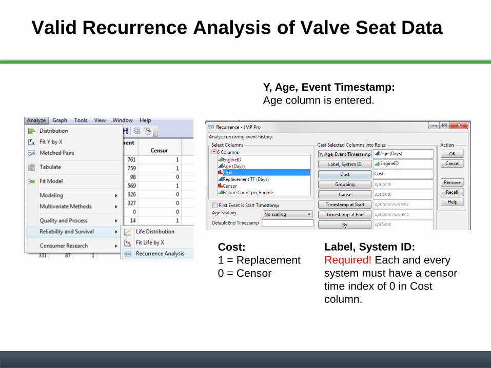
Valid Recurrence Analysis of Valve Seat Data
Cost:
1 = Replacement
0 = Censor
Label, System ID:
Required! Each and every
system must have a censor
time index of 0 in Cost
column.
Y, Age, Event Timestamp:
Age column is entered.

Valid Analysis of Valve Seats on Locomotive as
Repairable Systems
MCF plot shows repair rates increasing at a nearly
constant rate until around 550 days, when the rate
appears to increase. Is wearout occurring?

Comparison of Interarrival Times Vs. Ages
Note that several interarrival times of short duration occurring at oldest system ages show
up as early failures when order is neglected, resulting in misleading interpretation of data.

Analysis of Recurrence Rates (RR)
One desirable feature for implementation in the JMP
Recurrence Analysis platform would be the ability to display a
graph of the derivative or recurrence rate (RR) of the MCF. [7]
It is possible to numerically differentiate the MCF by placing a
variable length tangent on the curve and determining the slope
at the midpoint of the tangent. The length of the tangent is
determined by the number of data points included in the slope
calculation. The tangent is incremented sequentially by one
point for each group of points along the curve. [8]
Such a calculation is illustrated for a 23-point slope next.
Page 51

Numerical Differentiation of MCF Curve
Increasing the lengths of tangents smooths out the RR.
Page 52
MCF RR
Since we’re assuming replacement seals are identical, the RR graph shows an apparent
increasing recurrence rate after 550 days, possibly indicative of the onset of wearout.

Survival Distribution of Censoring Ages
Another feature that would be useful is a plot of the number
or percent of starting systems that exist as a function of
the system ages, that is, a plot of the number of censored
observations versus the censoring ages of the systems.
Page 53
Two locomotives began operation
over three months earlier than
practically all other systems. Both
systems had no replacement
failures.
One locomotive (#409) began
operation over six months later than
most systems. Nelson [3] reports
that this system was “dropped into
the water while being loaded on
shipboard to go to China. Water
removal and other cleanup delayed
its start in service.” #409 had three
replacements in this shortened time.

Calendar Date MCF Analysis (CMCF)
Normally an MCF is plotted versus the systems ages. However,
there may be applications where the MCF could be plotted versus
the calendar date to reveal issues that might be less evident by a
typical MCF calculation. [7]
For example, suppose a group of systems installed at various times
in a facility during the year are moved on the same date to a new
location. There may be multiple failures on or after the same date
associated with the move and not related to system ages.
As another example, a group of systems with different ages may all
receive a software upgrade that causes issues. Again, the
calendar date plot might be more revealing of a special cause
variation on the common date.
Page 54

Addition of Test for Detecting Trends
Against HPP Model
Laplace Test [2]
• Tests whether the ordered system ages at failure are
independent and uniformly distribution across an interval.
Reverse Arrangement Test [2]
• Tests if the interarrival times are randomly distributed for a
single system.
Page 55

JMP Fit Model for Recurrence Data Report
There are four parametric model choices. Since the field conditions are assumed similar,
we do not enter any effects, such as EnginerID, or if available, vintage year, temperature,
etc. Start with the simplest model, which is Homogeneous Poisson Process, HPP
(constant MTBF). .
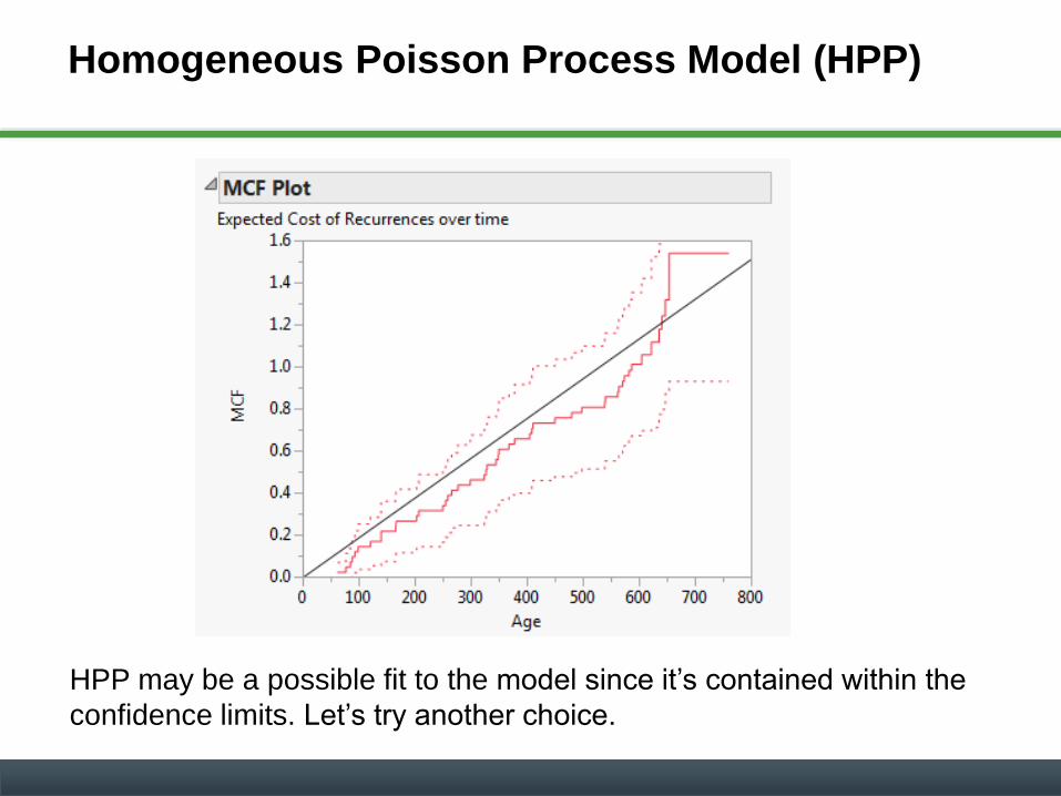
Homogeneous Poisson Process Model (HPP)
HPP may be a possible fit to the model since it’s contained within the
confidence limits. Let’s try another choice.

Power Nonhomogeneous Poisson Process
Model (PNHPP)
The PNHPP model appears to fit the data better. JMP has a homogeneity
test against the HPP model.
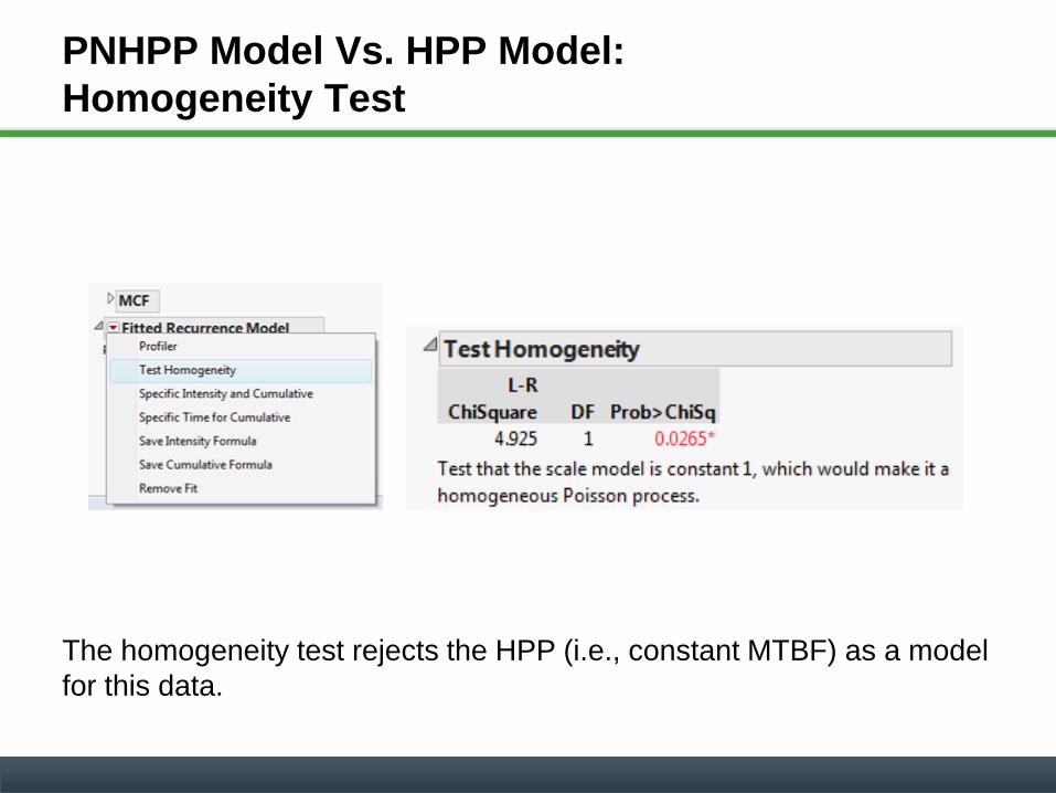
PNHPP Model Vs. HPP Model:
Homogeneity Test
The homogeneity test rejects the HPP (i.e., constant MTBF) as a model
for this data.

PNHPP Model: Intensity and Cumulative
Replacements at a Specific Age
The model predicts a cumulative number of replacements of ~2.3 at 1,000 days.

PNHPP Model: Ages to Specific Cumulative
Number of Replacements
Right click on table and select “Make Combined Data Table”.
Repeat for Number of
recurrences 2,3,4,5

PNHPP Model: Combined Table with Ages to
Specific Cumulative Number of Replacements
Combined Data Table with first two rows deleted.

PNHPP Model: Predictions of Cumulative
Repairs and Ages to Cumulative Repairs
Cumulative Repairs Vs. Ages Ages Vs. Cumulative Repairs

Are Systems Getting Better or Worse?
Add Delta column to Combined Data
Table and enter Row, Dif formula.
In contrast to the lognormal analysis of
interarrival times, which showed a
decreasing failure rate, the recurrence
analysis shows the times between failures are
predicted to become shorter indicating that
repairs will become more frequent with
increasing age.
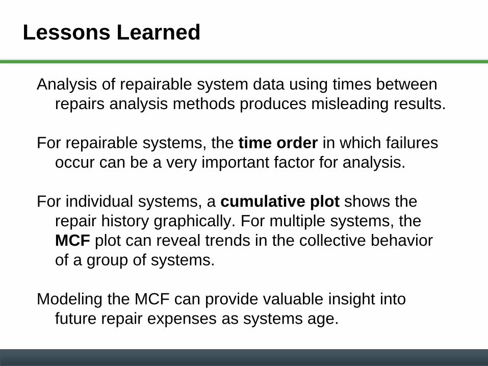
Lessons Learned
Analysis of repairable system data using times between
repairs analysis methods produces misleading results.
For repairable systems, the time order in which failures
occur can be a very important factor for analysis.
For individual systems, a cumulative plot shows the
repair history graphically. For multiple systems, the
MCF plot can reveal trends in the collective behavior
of a group of systems.
Modeling the MCF can provide valuable insight into
future repair expenses as systems age.

References
1. SAS Institute Inc. 2015. JMP® 12 Reliability and Survival Methods. Cary, NC:
SAS Institute Inc.
2. Tobias, P.A. and Trindade, D.C. 2012 Applied Reliability, 3rd ed., Boca Raton,
FL: CRC Press
3. Nelson, W.B. 2003. Recurrent Event Data Analysis for Product Repairs,
Disease Recurrence, and Other Applications. Philadelphia, PA:SIAM
4. Meeker, W.Q. and Escobar, L.A. 1998, Statistical Methods for Reliability Data,
New York: John Wiley & Sons
5. Davis, D.J. 1952, An analysis of some failure data. J Am Stat Soc 47:113-50
6. Nelson, W.B. 1995 Confidence limits for recurrence data – applied to cost or
number of product repairs. Technometrics 37:147-157
7. Trindade, D.C. and Nathan, S., 2008 Field Data Analysis for Repairable
Systems: Status and Industry Trends, Handbook of Performability
Engineering, London, Springer-Verlag
8. Trindade, D.C. 1975 An APL program to numerically differentiate data. IBM
TR Report (19.0361)
Page 66