Analysis of macular OCT images using deformable registration · Analysis of macular OCT images using deformable registration ... M. Hauser, E. S. Sotirchos, P. A. Calabresi, H. S

Analysis of macular OCT images usingdeformable registration

Min Chen,1,2,* Andrew Lang,1 Howard S. Ying,3 Peter A. Calabresi, 4

Jerry L. Prince,1 and Aaron Carass1

1Department of Electrical and Computer Engineering, The Johns Hopkins University,Baltimore, MD, 21218, USA

2Translational Neuroradiology Unit, National Institute of Neurological Disorders and Stroke,Bethesda, MD 20892, USA

3Wilmer Eye Institute, The Johns Hopkins School of Medicine, Baltimore, MD 21287, USA4Department of Neurology, The Johns Hopkins School of Medicine,

Baltimore, MD 21287, USA∗[email protected]

Abstract: Optical coherence tomography (OCT) of the macula has becomeincreasingly important in the investigation of retinal pathology. However,deformable image registration, which is used for aligning subjects forpairwise comparisons, population averaging, and atlas label transfer, has notbeen well–developed and demonstrated on OCT images. In this paper, wepresent a deformable image registration approach designed specifically formacular OCT images. The approach begins with an initial translation to alignthe fovea of each subject, followed by a linear rescaling to align the top andbottom retinal boundaries. Finally, the layers within the retina are aligned bya deformable registration using one-dimensional radial basis functions. Thealgorithm was validated using manual delineations of retinal layers in OCTimages from a cohort consisting of healthy controls and patients diagnosedwith multiple sclerosis (MS). We show that the algorithm overcomes theshortcomings of existing generic registration methods, which cannot bereadily applied to OCT images. A successful deformable image registrationalgorithm for macular OCT opens up a variety of population based analysistechniques that are regularly used in other imaging modalities, such asspatial normalization, statistical atlas creation, and voxel based morphometry.Examples of these applications are provided to demonstrate the potentialbenefits such techniques can have on our understanding of retinal disease. Inparticular, included is a pilot study of localized volumetric changes betweenhealthy controls and MS patients using the proposed registration algorithm.

© 2014 Optical Society of AmericaOCIS codes: (100.0100) Image processing; (170.4470) Ophthalmology; (170.4500) Opticalcoherence tomography.

References and links1. J. G. Fujimoto, W. Drexler, J. S. Schuman, and C. K. Hitzenberger, “Optical coherence tomography (OCT) in

ophthalmology: Introduction,” Opt. Express 17, 3978–3979 (2009).2. E. M. Frohman, J. G. Fujimoto, T. C. Frohman, P. A. Calabresi, G. Cutter, and L. J. Balcer, “Optical coherence

tomography: A window into the mechanisms of multiple sclerosis,” Nat. Clin. Pract. Neuro. 4, 664–675 (2008).3. J. N. Ratchford, S. Saidha, E. S. Sotirchos, J. A. Oh, M. A. Seigo, C. Eckstein, M. K. Durbin, J. D. Oakley, S. A.

Meyer, A. Conger, T. C. Frohman, S. D. Newsome, L. J. Balcer, E. M. Frohman, and P. A. Calabresi, “Active MSis associated with accelerated retinal ganglion cell/inner plexiform layer thinning,” Neurology 80, 47–54 (2013).

#210228 - $15.00 USD Received 21 Apr 2014; revised 30 May 2014; accepted 2 Jun 2014; published 11 Jun 2014(C) 2014 OSA 1 July 2014 | Vol. 5, No. 7 | DOI:10.1364/BOE.5.002196 | BIOMEDICAL OPTICS EXPRESS 2196

4. S. Saidha, E. S. Sotirchos, J. Oh, S. B. Syc, M. A. Seigo, N. Shiee, C. Eckstein, M. K. Durbin, J. D. Oakley, S. A.Meyer, T. C. Frohman, S. Newsome, J. N. Ratchford, L. J. Balcer, D. L. Pham, C. M. Crainiceanu, E. M. Frohman,D. S. Reich, and P. A. Calabresi, “Relationships between retinal axonal and neuronal measures and global centralnervous system pathology in Multiple Sclerosis,” JAMA Neurology 70, 34–43 (2013).

5. P. A. Keane, P. J. Patel, S. Liakopoulos, F. M. Heussen, S. R. Sadda, and A. Tufail, “Evaluation of age-relatedmacular degeneration with optical coherence tomography,” Surv. Ophthalmol. 57, 389–414 (2012).

6. G. Querques, R. Lattanzio, L. Querques, C. Del Turco, R. Forte, L. Pierro, E. H. Souied, and F. Bandello,“Enhanced depth imaging optical coherence tomography in Type 2 diabetes,” Invest. Ophthalmol. Vis. Sci. 53,6017–6024 (2012).

7. Y. Lu, Z. Li, X. Zhang, B. Ming, J. Jia, R. Wang, and D. Ma, “Retinal nerve fiber layer structure abnormalities inearly Alzheimer’s disease: Evidence in optical coherence tomography,” Neurosci. Lett. 480, 69–72 (2010).

8. M. E. Hajee, W. F. March, D. R. Lazzaro, A. H. Wolintz, E. M. Shrier, S. Glazman, and I. G. Bodis-Wollner,“Inner retinal layer thinning in Parkinson disease,” Arch. Ophthalmol. 127, 737–741 (2009).

9. V. Guedes, J. S. Schuman, E. Hertzmark, G. Wollstein, A. Correnti, R. Mancini, D. Lederer, S. Voskanian,L. Velazquez, H. M. Pakter, T. Pedut-Kloizman, J. G. Fujimoto, and C. Mattox, “Optical coherence tomographymeasurement of macular and nerve fiber layer thickness in normal and glaucomatous human eyes,” Ophthalmology110, 177–189 (2003).

10. D. Koozekanani, K. Boyer, and C. Roberts, “Retinal thickness measurements from optical coherence tomographyusing a Markov boundary model,” IEEE Trans. Med. Imag. 20, 900–916 (2001).

11. H. Ishikawa, D. M. Stein, G. Wollstein, S. Beaton, J. G. Fujimoto, and J. S. Schuman, “Macular segmentationwith optical coherence tomography,” Invest. Ophthalmol. Vis. Sci. 46, 2012–2017 (2005).

12. M. K. Garvin, M. D. Abramoff, X. Wu, S. R. Russell, T. L. Burns, and M. Sonka, “Automated 3-D intraretinallayer segmentation of macular spectral-domain optical coherence tomography images,” IEEE Trans. Med. Imag.28, 1436–1447 (2009).

13. S. J. Chiu, X. T. Li, P. Nicholas, C. A. Toth, J. A. Izatt, and S. Farsiu, “Automatic segmentation of seven retinallayers in SDOCT images congruent with expert manual segmentation,” Opt. Express 18, 19413–19428 (2010).

14. A. Lang, A. Carass, E. Sotirchos, and J. L. Prince, “Segmentation of retinal OCT images using a random forestclassifier,” in “Proc. SPIE-MI 2013,” (Lake Buena Vista, FL, 2013).

15. A. Lang, A. Carass, M. Hauser, E. S. Sotirchos, P. A. Calabresi, H. S. Ying, and J. L. Prince, “Retinal layersegmentation of macular OCT images using boundary classification,” Biomed. Opt. Express 4, 1133–1152 (2013).

16. A. Sotiras, C. Davatzikos, and N. Paragios, “Deformable medical image registration: A survey.” IEEE Trans. Med.Imag. 32, 1153–1190 (2013).

17. M. I. Miller, G. E. Christensen, Y. Amit, and U. Grenander, “Mathematical textbook of deformable neuroanatomies,”Proc. Natl. Acad. Sci. 90, 11944–11948 (1993).

18. J. Ashburner and K. J. Friston, “Voxel-based morphometry—the methods,” NeuroImage 11, 805821 (2000).19. B. B. Avants, C. L. Epstein, M. Grossman, and J. C. Gee, “Symmetric diffeomorphic image registration with

cross-correlation: Evaluating automated labeling of elderly and neurodegenerative brain,” Med. Image Anal. 12,26–41 (2008).

20. M. Auer, P. Regitnig, and G. A. Holzapfel, “An automatic nonrigid registration for stained histological sections,”IEEE Trans. Imag. Proc. 14, 475–486 (2005).

21. K. K. Brock, M. B. Sharpe, L. A. Dawson, S. M. Kim, and D. A. Jaffray, “Accuracy of finite element model-basedmulti-organ deformable image registration,” Med. Phys. 32, 1647–1659 (2005).

22. W. Bai and M. Brady, “Motion correction and attenuation correction for respiratory gated PET images,” IEEETrans. Med. Imag. 30, 351–365 (2011).

23. T. M. Jørgensen, J. Thomadsen, U. Christensen, W. Soliman, and B. Sander, “Enhancing the signal-to-noise ratioin ophthalmic optical coherence tomography by image registration—method and clinical examples,” J. Biomed.Opt. 12, 041208–041208 (2007).

24. J. Xu, H. Ishikawa, G. Wollstein, L. Kagemann, and J. S. Schuman, “Alignment of 3-d optical coherencetomography scans to correct eye movement using a particle filtering,” IEEE Trans. Med. Imag. 31, 1337–1345(2012).

25. Y. M. Liew, R. A. McLaughlin, F. M. Wood, and D. D. Sampson, “Motion correction of in vivo three-dimensionaloptical coherence tomography of human skin using a fiducial marker,” Biomed. Opt. Express 3, 1774 (2012).

26. A. Giani, M. Pellegrini, A. Invernizzi, M. Cigada, and G. Staurenghi, “Aligning scan locations from consecutivespectral-domain optical coherence tomography examinations: A comparison among different strategies,” Invest.Ophthalmol. Vis. Sci. 53, 7637–7643 (2012).

27. M. Niemeijer, M. K. Garvin, K. Lee, B. van Ginneken, M. D. Abramoff, and M. Sonka, “Registration of 3Dspectral OCT volumes using 3D SIFT feature point matching,” in “Proc. SPIE-MI 2009,” (Lake Buena Vista, FL,2009).

28. M. Niemeijer, K. Lee, M. K. Garvin, M. D. Abramoff, and M. Sonka, “Registration of 3D spectral OCT volumescombining ICP with a graph-based approach,” in “Proc. SPIE-MI 2012,” (San Diego, CA, 2012).

29. A. A. Goshtasby, 2-D and 3-D Image Registration: For Medical, Remote Sensing, and Industrial Applications(Wiley, 2005).


30. E. A. Maguire, D. G. Gadian, I. S. Johnsrude, C. D. Good, J. Ashburner, R. S. J. Frackowiak, and C. D. Frith,“Navigation-related structural change in the hippocampi of taxi drivers,” Proc. Nat. Acad. Sci. 97, 4398–4403(2000).

31. C. D. Good, I. S. Johnsrude, J. Ashburner, R. N. A. Henson, K. J. Friston, and R. S. J. Frackowiak, “A voxel-basedmorphometric study of ageing in 465 normal adult human brains,” NeuroImage 14, 21–36 (2001).

32. A. F. Goldszal, C. Davatzikos, D. Pham, M. X. H. Yan, R. N. Bryan, and S. M. Resnick, “An image-processingsystem for qualitative and quantitative volumetric analysis of brain images,” J. Computer Assisted Tomography22, 827–837 (1998).

33. C. Davatzikos, A. Genc, D. Xu, and S. M. Resnick, “Voxel-based morphometry using the RAVENS maps: Methodsand validation using simulated longitudinal atrophy,” NeuroImage 14, 1361–1369 (2001).

34. S. M. Resnick, D. L. Pham, M. A. Kraut, A. Zonderman, and C. Davatzikos, “Longitudinal magnetic resonanceimaging studies of older adults: A shrinking brain,” J. Neurosci. 23, 3295–3301 (2003).

35. M. Chen, A. Lang, E. Sotirchos, H. S. Ying, P. A. Calabresi, J. L. Prince, and A. Carass, “Deformable registrationof macular oct using a-mode scan similarity,” in “Biomedical Imaging (ISBI), 2013 IEEE 10th InternationalSymposium on,” (IEEE, 2013), pp. 476–479.

36. E. Gibson, M. Young, M. V. Sarunic, , and M. F. Beg, “Optic nerve head registration via hemispherical surfaceand volume registration,” IEEE Trans. Biomed. Eng. 57, 2592–2595 (2010).

37. B. Antony, M. D. Abramoff, L. Tang, W. D. Ramdas, J. R. Vingerling, N. M. Jansonius, K. Lee, Y. H. Kwon,M. Sonka, and M. K. Garvin, “Automated 3-D method for the correction of axial artifacts in spectral-domainoptical coherence tomography images,” Biomed. Opt. Express 2, 2403–2416 (2011).

38. Y. Zheng, R. Xiao, Y. Wang, and J. C. Gee, “A generative model for oct retinal layer segmentation by integratinggraph-based multi-surface searching and image registration,” in “16th International Conference on Medical ImageComputing and Computer Assisted Intervention (MICCAI 2013),” (Springer, 2013), pp. 428–435.

39. Y. Ou, A. Sotiras, N. Paragios, and C. Davatzikos, “Dramms: Deformable registration via attribute matching andmutual-saliency weighting,” Med. Image Anal. 15, 622–639 (2011).

40. A. N. Kuo, R. P. McNabb, S. J. Chiu, M. A. El-Dairi, S. Farsiu, C. A. Toth, and J. A. Izatt, “Correction of ocularshape in retinal optical coherence tomography and effect on current clinical measures,” Am. J. Ophthalmol.156,304–311 (2013).

41. G. K. Rohde, A. Aldroubi and B. M. Dawant, “The adaptive bases algorithm for intensity based nonrigid imageregistration,” IEEE Trans. Med. Imag. 22, 1470–1479 (2003).

42. A. Guimond, J. Meunier, and J.-P. Thirion, “Average brain models: A convergence study,” Computer vision andimage understanding 77, 192–210 (2000).

43. B. Avants and J. C. Gee, “Geodesic estimation for large deformation anatomical shape averaging and interpolation,”NeuroImage 23, S139–S150 (2004).

44. S. Khullar, A. M. Michael, N. D. Cahill, K. A. Kiehl, G. Pearlson, S. A. Baum, and V. D. Calhoun, “ICA-fNORM:Spatial normalization of fMRI data using intrinsic group-ICA networks,” Front. Syst. Neurosci 5 (2011).

45. D. Rueckert, A. F. Frangi, and J. A. Schnabel, “Automatic construction of 3-d statistical deformation models ofthe brain using nonrigid registration,” IEEE Trans. Med. Imag. 22, 1014–1025 (2003).

46. M. Chen, A. Carass, D. Reich, P. Calabresi, D. Pham, and J. Prince, “Voxel-wise displacement as independentfeatures in classification of multiple sclerosis.” in “Proc. SPIE-MI 2013,” (Lake Buena Vista, FL, 2013).

47. S. Gerber, T. Tasdizen, P. T. Fletcher, S. Joshi, and R. Whitaker, “Manifold modeling for brain population analysis,”Med. Image Anal. 14, 643–653 (2010).

48. Y. Fan, S. M. Resnick, X. Wu, and C. Davatzikos, “Structural and functional biomarkers of prodromal Alzheimer’sdisease: A high-dimensional pattern classification study,” NeuroImage 41, 277–285 (2008).

49. S. Saidha, E. S. Sotirchos, M. A. Ibrahim, C. M. Crainiceanu, J. M. Gelfand, Y. J. Sepah, J. N. Ratchford, J. Oh,M. A. Seigo, S. D. Newsome, L. J. Balcer, E. M. Frohman, A. J. Green, Q. D. Nguyen, and P. A. Calabresi,“Microcystic macular oedema, thickness of the inner nuclear layer of the retina, and disease characteristics inmultiple sclerosis: A retrospective study,” The Lancet Neurology 11, 963–972 (2012).

50. A. Klein, S. S. Ghosh, B. Avants, B. T. T. Yeo, B. Fischl, B. Ardekani, J. C. Gee, J. J. Mann, and R. V. Parsey,“Evaluation of volume-based and surface-based brain image registration methods,” NeuroImage 51, 214–220(2010).

51. B. B. Avants, N. J. Tustison, G. Song, P. A. Cook, A. Klein, and J. C. Gee, “A reproducible evaluation of ANTssimilarity metric performance in brain image registration,” NeuroImage 54, 2033–2044 (2011).

52. L. R. Dice, “Measures of the amount of ecologic association between species,” Ecology 26, 297–302 (1945).53. K. J. Friston, J. Ashburner, S. Kiebel, T. Nichols, and W. Penny, eds., Statistical Parametric Mapping: The Analysis

of Functional Brain Images (Academic Press, 2007).54. J. B. Kerrison, T. Flynn, and W. R. Green, “Retinal pathologic changes in multiple sclerosis,” Retina 14, 445–451

(1994).55. A. J. Green, S. McQuaid, S. L. Hauser, I. V. Allen, and R. Lyness, “Ocular pathology in multiple sclerosis: retinal

atrophy and inflammation irrespective of disease duration,” Brain 133, 1591–1601 (2010).56. B. J. Lujan, A. Roorda, R. W. Knighton, and J. Carroll, “Revealing henle’s fiber layer using spectral domain

optical coherence tomography,” Invest. Ophthalmol. Visual Sci. 52, 1486–1492 (2011).


57. B. C. Lucas, J. A. Bogovic, A. Carass, P.-L. Bazin, J. L. Prince, D. L. Pham, and B. A. Landman, “The Java ImageScience Toolkit (JIST) for rapid prototyping and publishing of neuroimaging software,” Neuroinformatics 8, 5–17(2010).

1. Introduction

Optical coherence tomography (OCT) is an imaging technology that enables objective analysisof the mechanisms of neurodegeneration in an important, yet isolated, portion of the centralnervous system—the retina. It presents cellular level descriptions by providing micrometer (µm)resolution imaging of the retina based on the optical scattering properties of biological tissues.OCT offers several other distinguishing advantages such as patient comfort, ease of use, noionizing radiation, quick acquisition, and low cost. These properties have allowed the ophthalmiccommunity to better explore the retinal cell layers within the macula [1]. OCT has been particu-larly useful in the assessment and characterization of multiple sclerosis (MS) through the analysisof the thickness of various retinal layers [2–4]. It has also seen use for exploring numerous otherdiseases, including age-related macular degeneration [5], diabetes [6], Alzheimer’s disease [7],Parkinson’s disease [8], and glaucoma [9].

While automated and semi-automated methods for analyzing and segmenting retinal layersin OCT have been introduced regularly over the past decade [10–15], there has been very littledevelopment of image registration methods for OCT. Image registration is the task of trans-forming different images into the same geometric space or coordinate system. This allows forboth intersubject registration, the alignment of images from different subjects, and longitudinalregistration, the alignment of multiple images from the same subject at different time points.There has been extensive literature surrounding image registration and its application in medicalimaging [16]. It has been widely used in a variety of neuroanatomy settings [17–19] and forvarious vital organs [20–22]. Despite this rich history, the development of registration techniquesin OCT has been relatively limited. Existing works are restricted almost exclusively to rigidregistrations [23–28], where only rigid body transformations are allowed in the alignment. Suchtransformation models are generally inadequate for the retina, since the differences betweenretinal layers from different subjects (or even the same subject over time) cannot be fully repre-sented by such a low-dimensional model. To capture these differences, an affine or deformableregistration is necessary, where affine or nonlinear freeform transformations are used in themodel, respectively. Deformable registration is also divided into subgroups, including parametricmodels which represent transformations using basis functions, and physical models, which usetransformations allowed in elastic, viscous, or viscoelastic materials. Each of these subgroupshave their own strengths and weaknesses (see [29] for a detailed discussion).

One potential application of retinal OCT registration is to combine macular scans from apopulation of subjects to create a macular stereotaxic space, often referred to as a normalizedspace, which can serve as a standard reference space for comparing between different subjects.Such a space directly enables a number of advanced analytic techniques such as voxel basedmorphometry (VBM) [18], which allows the exploration of local tissue composition differencesbetween two populations, and has seen extensive use in analyzing functional and structuraldifferences in the brain [30, 31]. A normalized space can also be used to study localizedvolumetric changes between populations, for example, by using the Regional Analysis ofVolumes Examined in Normalized Space (RAVENS) [32, 33] method. RAVENS has been usedto accurately quantify localized volume differences in the brain [34], and readily generatesvisualizations, called RAVENS maps, of the difference between two populations. The techniqueuses the deformations learned from each subject registration to compute the local expansionsand contractions of tissue volume relative to the normalized space. In retinal OCT, these types


of analyses can allow local investigation of layer volume changes, which is not possible fromsolely examining layer thickness calculations from segmentation results.

To our knowledge, excluding our own preliminary work [35], only three other algorithms havebeen reported that apply a nonlinear deformable model to register retinal OCT data. Gibson etal. [36] presented a method that segments and extracts the optic nerve head surface from the OCTimage, and then registers the surfaces using a combined surface and volumetric registration. Themethod was validated by comparing the overlap of the optical nerve head after the registration.Antony et al. [37] introduced a method where the surface between the inner and outer segmentsof the photoreceptor cells are used with a thin-plate spline to correct for axial artifacts. Lastly,Zheng et al. [38] presented a segmentation approach that uses the SyN [19] registration algorithmto aid in segmentation. The method uses approximate segmentations of the retinal layers todivide the image into regions, and then registers each region individually with training data toestimate a more accurate segmentation. Of these three methods, only Gibson et al. provided aninter-subject registration that allows for the construction of a normalized space and populationanalysis. The other two methods primarily used the registration internally to aid their distortioncorrection and segmentation algorithm. All three of these deformable registration methodsrequired a segmentation of the OCT data to guide the registration algorithm. This requirementrestricts the registration accuracy to that of the segmentation. Since OCT segmentations onlyprovide information about the positions of layer boundaries, these registration algorithms arepotentially inaccurate within the segmented regions.

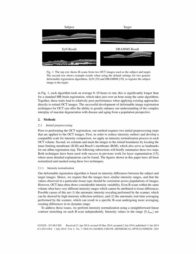
Intensity-based volumetric registration, i.e., where the alignment is performed by matchingthe voxel intensities between the two images, is an alternative to existing segmentation-basedmethods. To our knowledge, the only intensity-based volumetric deformable registration that hasbeen developed and validated specifically on macular OCT images is our preliminary work [35].There are a number of generic volumetric registration algorithms (most of which were developedfor brain image registration) that can be applied to OCT data. However, our investigations havefound that such algorithms tend to be unreliable when applied to the whole OCT image, withoutseparating and registering individual layers as in Zheng et al [38]. Figure 1 shows two OCTimages and the results of registering a subject image to a target image using both SyN [19] andDRAMMS [39], two highly-rated deformable registration algorithms developed for brain imageregistration, with default settings.

The lack of deformable registration tools for retinal OCT can be attributed to several factors.First, OCT (particularly spectral-domain OCT) is a relatively new modality in comparisonto other medical imaging modalities such as magnetic resonance imaging (MRI), computedtomography, and ultrasound. Hence, the demand and necessity for algorithms and techniquesdesigned for OCT images is fairly recent. Second, there are a number of characteristics inherentto OCT images which make adaptation and development of existing registration algorithmschallenging. These characteristics include poor signal-to-noise ratio (SNR) in comparison toother imaging modalities, which makes it difficult for intensity based methods to find correct cor-respondences. The data is often extremely anisotropic, where the gap between the cross-sectionalslices (B-scans) can be upwards of 30 times larger than the resolution within each B-scan. Thisis generally not compatible with the regularization inherent in most transformation models inexisting algorithms, and also creates significant challenges when performing interpolation. Third,the geometry of OCT images are not well defined between different subjects. The scan lines(A-scans) in the images are generally represented parallel to each other, while physically theyshould be fanning outwards from the center [40]. Since this geometry is specific to the optics ofeach individual’s eye, it is unclear how transformations between retinal OCT images should beperformed, particularly when deforming across different A-scans. Finally, the high resolution ofOCT images create a large data size that poses a computational challenge. In the examples shown


Subject Target

SyN Result DRAMMS Result

Fig. 1. The top row shows B-scans from two OCT images used as the subject and target.The second row shows example results when using the default settings for two genericdeformable registration algorithms, SyN [19] and DRAMMS [39], to register the subjectimage to the target.

in Fig. 1, each algorithm took on average 8–10 hours to run; this is significantly longer thanfor a standard MR brain registration, which takes just over an hour using the same algorithms.Together, these traits lead to relatively poor performance when applying existing approachesdirectly to retinal OCT images. The successful development of deformable image registrationtechniques for OCT can offer the ability to greatly enhance our understanding of the complexinterplay of macular degeneration with disease and aging from a population perspective.

2. Methods

2.1. Initial preprocessing

Prior to performing the OCT registration, our method requires two initial preprocessing stepsthat are applied to the OCT images. First, in order to reduce intensity outliers and develop acompatible scale for intensity comparison, we apply an intensity normalization process to eachOCT volume. Second, we estimate and mask the images to the retinal boundaries by locating theinner limiting membrane (ILM) and Bruch’s membrane (BrM), which also serve as landmarksfor our affine registration step. The following subsections will briefly summarize these two steps.Both techniques have been used with success in previous work for layer segmentation [15],where more detailed explanations can be found. The figures shown in this paper have all beennormalized and masked using these two techniques.

2.1.1. Intensity normalization

Our deformable registration algorithm is based on intensity differences between the subject andtarget images. Hence, we require that the images have similar intensity ranges, and that thevalues observed in a particular tissue type should be consistent across populations of images.However, OCT data often shows considerable intensity variability. Even B-scans within the samevolume often have very different intensity ranges which cannot be attributed to tissue differences.Possible causes of this are (1) the automatic intensity rescaling performed by the scanner, whichcan be skewed by high intensity reflection artifacts, and (2) the automatic real-time averagingperformed by the scanner, which can result in a specific B-scan undergoing more averaging,creating differences in its dynamic range.

To address these issues, we perform intensity normalization using a straightforward linearcontrast stretching on each B-scan independently. Intensity values in the range [0, Imax] are


linearly rescaled to [0,1], with values larger than Imax being capped at the maximum. The cutoff,Imax, is determined robustly by first median-filtering each individual A-scan within the sameB-scan with a kernel size of 15 pixels (58 µm), and then setting Imax as 5% larger than themaximum intensity in the median filtered image.

2.1.2. Retinal boundary detection and fovea localization

Our next preprocessing step is estimating and masking the images to the top and bottom bound-aries of the retina, which are defined by the ILM and BrM, respectively. These retinal extentsare found in the following manner. Each B-scan is independently Gaussian smoothed (σ = 3pixels which is σ(x,y) = (17,12) µm), followed by an image gradient computation along eachA-scan using a Sobel kernel. In each A-scan, the two largest positive gradient values that aremore than 25 pixels (97 µm) apart are taken as initial estimates of either the ILM or the innersegment (IS) outer segment (OS) boundary. We estimate the BrM, by searching up to 30 pixels(116 µm) below the IS-OS boundary for the largest negative gradient. These boundary estimatesare refined by comparing to the median filtered collection of the gradients, and then Gaussiansmoothing the result. Using this detection, we mask out non-retinal material and approximatethe location of the fovea as the superior point of the thinnest portion of the retina within a searchwindow at the center of the image.

2.2. Image registration method

The primary goal of image registration is to estimate a transformation that maps correspondinglocations between a subject image S(x′) and a target image T (x). Here, x′ = (x′,y′,z′) andx = (x,y,z) describe 3D coordinates in the subject and target image domains, DS and DT ,respectively, and S(x′) and T (x) are the intensities of each image at those coordinates. For ourOCT images, we assign the x, y, and z axes as the lateral, through-plane, and axial directions,respectively. This makes A-scan lines parallel to the z axis and B-scans as images parallel to thexz–plane.

We describe the transformation that the registration algorithm is attempting to solve as themapping v : DT → DS. This is generally represented as a pullback vector field, v(x), where thevectors are rooted in the target domain and point to locations in the subject domain. The field isapplied to S(x′) by pulling subject image intensities into the target domain. This produces theregistration result, a transformed subject image, S, defined as

S(x) = S(v(x)) , ∀x ∈ DT , (1)

which has coordinates in the target domain. The goal of the registration algorithm is to findv such that the images S and T are as similar as possible. This is performed by minimizing acost function that evaluates how similar the intensities in S(v(x)) are to T (x) at each x, whileconstraining the transformation to be smooth and continuous (i.e., physically sensible).

As described in Section 1, the two major challenges of retinal OCT registration are (1) theimage voxels tend to be highly anisotropic, and (2) the physical geometry of the image is notproperly defined by how the A-scans are presented in the OCT. The former makes regularizationand interpolation difficult, if not infeasible, for images with large B-scan separations. The latterobfuscates our ability to apply a sensible deformation that respects the physical space beingimaged. This is particularly problematic when attempting to apply a deformation that crossesmultiple A-scans. For example, a deformation parallel to the x or y axes in the OCT image isactually curved in physical space. The amount of curvature depends on the fanning of the A-scanduring the acquisition, which depends on the optics of the eye being imaged. Such informationis often not acquired with the OCT, which makes the actual deformation applied in the physicalspace ambiguous.


To address these concerns, we impose strong restrictions on the class of transformations ourregistration is allowed to estimate. In the x (lateral) and y (through-plane) directions, we permitonly discrete translations such that A-scans from the subject always coincide with A-scans inthe target (except for missing scans at the boundaries). This removes the need to interpolateintensities between two A-scans or two B-scans. Non-rigid transformations are only allowed inthe z (axial) direction and will be constructed as a composition of individual (A-scan to A-scan)affine and deformable registration steps. This will permit accurate alignment of the features ineach A-scan, including the retinal layers.

Our overall registration result is the composition of three steps: a 2D global translation of thewhole volume (using discrete offsets only), a set of 1D affine transformations applied to each A-scan, and a set of 1D deformable transformations applied to each A-scan. These transformationsare learned and applied in stages and then composed to construct the total 3D transformationv. Let r represent the 2D global translation, and let ai, j and di, j represent, respectively, the 1Daffine and 1D deformable transformations applied to the A-scan indexed by the discrete x and ycoordinates, m = (i, j). We can write the total transformation as v(x) = r◦am ◦dm(x), whereit is assumed that x belongs to the A-scan indexed by m. The deformed subject image in thetemplate space is then given by

S(x) = S(r(am(dm(x)))) , ∀x ∈ DT . (2)

In the following sections we present the method to carry out each of these steps.

2.2.1. 2D global translation

The goal of the 2D global translation is to align the subject such that its fovea is aligned withthe same A-scan as the fovea in the target image. Let the positions of the foveae in the subjectand target images be denoted by fS and fT , respectively. These locations are found using theapproach described in Section 2.1.2, which forces them to be located within A-scans in the twoimages. The rigid transformation is therefore described by

r(x) = x− t , (3)

where

t =

(fS)x− (fT )x

(fS)y− (fT )y

0

. (4)

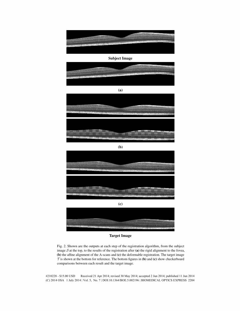
The notation (fS)x and (fS)y denote the x and y-components of fS, and likewise for (fT )x and(fT )y. Figure 2(a) shows an example of a result after applying just this rigid 2D foveal translationto the subject image.

2.2.2. 1D affine transformation

The 1D affine transformation step assumes that the foveae are aligned and will now considereach A-scan separately. The goal is to find the 1D affine transformation that matches the ILMand BrM boundary locations (both found in Section 2.1.2) between each pair of foveal alignedA-scans in the subject and target images. Since there are two landmarks and two unknowns ina 1D affine transformation, the solution can be written in closed form. For each A-scan m theILM and BrM boundaries are scalar locations along the A-scan. We refer to these as iS,m andbS,m for the subject image and iT ,m and bT ,m for the target image, respectively. The 1D affinetransformation for that A-scan is then given by

am(x) = Fmx+ tm, (5)


Subject Image

(a)

(b)

(c)

Target Image

Fig. 2. Shown are the outputs at each step of the registration algorithm, from the subjectimage S at the top, to the results of the registration after (a) the rigid alignment to the fovea,(b) the affine alignment of the A-scans and (c) the deformable registration. The target imageT is shown at the bottom for reference. The bottom figures in (b) and (c) show checkerboardcomparisons between each result and the target image.


where

Fm =

1 0 00 1 00 0 rm

, (6)

and

tm =

00

iS,m +bS,m

2− rm

(iT ,m +bT ,m

2

) . (7)

The scale factor, rm, is calculated from the ILM and BrM locations for each A-scan using

rm =(bS,m− iS,m)(bT ,m− iT ,m)

. (8)

We refer to the combination of the rigid translation step and this collection of 1D affine transfor-mations at each A-scan as our A-OCT registration. Figure 2(b) shows the resulting image afterapplying this step to the foveal aligned result.

2.2.3. 1D deformable transformation

Following the A-OCT registration, the next step in our algorithm is to use a 1D deformable reg-istration to further improve the alignment of the retinal layers. Unlike the 1D affine registration,where the transformation can be represented as a matrix, the deformable transformation dm foreach A-scan m is a free-form mapping at each x with the restriction that the deformation mustbe smooth and can only occur along the A-scan (z) direction. In this registration, dm is modeledas a summation of radial basis functions (RBFs), Φ(x), using

dm(x) = x+∑i

ciΦ(x−xi), (9)

where ci and xi determine the size and center of each RBF, respectively. For Φ(x), we choosethe same RBF as presented in [41], except with the deformation restricted only to the z direction:

Φ(x) =

00

φ

(‖x‖

s

) , where φ(r) = (1− r)4

+(3r3 +12r2 +16r+4), (10)

for (1− r)+ = max(1− r,0), which has support s. This RBF has several beneficial propertiessuch as smoothness, positive definiteness, and compact support. In addition, [41] showed thatgiven the correct constraints on the size of each RBF, dm is guaranteed to be homeomorphic. Ahomeomorphic deformation field allows the deformation to preserve the topology of the imageand prevent folding and tearing of the underlying anatomy in the image.

To solve for dm, the algorithm uniformly places the RBFs along the A-scan and then iterativelyminimizes the energy function

ESSDm = ∑

{x|(x,y)=m}(T (x)−S(A-OCT)(dm(x)))2

, (11)

which describes the intensity difference between the target image and the A-OCT result deformedby the current estimate of dm, across a particular A-scan. This is often referred to as the sum ofsquare differences (SSD) similarity measure.


One disadvantage of optimizing the deformation field between only pairs of A-scans is that itcan lead to discontinuities in the total deformation. It also ignores potentially useful neighboringinformation that can aid the optimization. To address this, we introduce a regularization term,

ERegm =

R

∑r=−Rr 6=0

∑{x|(x,y)=m+(r,0)}

1|r|

(T (x)−S(A-OCT)(dm(x)))2, (12)

where R is a parameter that determines how many adjacent A-scans, in the same B-scan, to usein the regularization. The current deformation dm is applied at each adjacent A-scan (m+(r,0))and then the function checks the SSD error produced by that deformation relative to the targetimage. Since we expect adjacent A-scans to be fairly continuous, if a deformation at m causeshuge errors in adjacent neighbors, then that deformation is heavily penalized. A weight term isincluded to reduce the contribution of comparisons made further away from m, since we expectthe deformation to be less applicable with distance.

We make two notes regarding this regularization term. First, the deformations of the adjacentA-scans with dm are only used for the optimization of the deformation at the current A-scan.The deformations are not applied permanently to the adjacent A-scans. When the algorithmmoves on to estimate a deformation at those adjacent A-scans, a new deformation is estimated.Second, the cost function does not regularize across B-scans, which follows our premise that thelarge separation between B-scans provide poor correspondences for the registration. Naturally,for data that do not suffer from this limitation, this regularization can be easily extended to usemultiple B-scans as well.

The two energy terms are summed (ESSD+EReg) to produce our total cost function, which weminimize at each A-scan to estimate dm. Brent’s 1D line search optimization method is used toperform this minimization. After evaluating dm at each A-scan, we have all the transformationsrequired to create the final registration result, S from Eq. 2, which represent the subject imageregistered to the target domain. Figure 2(c) shows an example of this final result. We refer to thecombination of all three registration steps as our D-OCT registration.

2.3. Constructing a normalized space using deformable registration

An important application of deformable registration is the ability to construct a normalized spacefor analyzing a population of subjects. The normalized space is a common target space to whichall images in a group of subjects are registered. This allows spatial correspondences betweenthe subjects to be observed and analyzed together as a population. Often, an average atlas isconstructed for this purpose, where the atlas represents the average anatomy of the population.Constructing such an atlas and using it as a normalized space via deformable registration is awell studied topic in brain MRI analysis. A number of methods have been proposed for creatingsuch a space [42–44]. In generating our normalized space, we follow the method presentedin [42] where the average atlas is found by iteratively registering each subject to an estimate ofthe average atlas, and then adjusting the atlas such that the average of all the deformations iscloser to zero.

2.4. Regional analysis of volumes examined in normalized space

The ability to construct a normalized space opens up numerous existing techniques for analyz-ing images from a population perspective, such as voxel based morphometry [18], statisticaldeformation models [45], tissue density maps [32], disease classification [46], and manifoldlearning [47]. To demonstrate this capability, we apply our registration approach in conjunctionwith the tissue density based analysis known as RAVENS. This voxel-wise analysis was intro-duced for neuroimaging in [32], and has been used to show localized brain volume changes in


Alzheimer’s disease [48]. It uses a tissue segmentation with the deformation learned from eachregistration to the normalized space to estimate the relative local volume changes between eachsubject and the atlas.

The relative local volume change is calculated by first taking each voxel in a segmentationand projecting it into the target space using the registration deformation fields. This processkeeps track of how each voxel is distributed by the projection and allows the method to recordthe degree of compression and expansion at each voxel that the segmentations had to undergoin order to be registered into the normalized space. As a result, we obtain localized measuresof volume changes for each subject relative to the average atlas. This provides the ability tolocate differences in relative volume changes between control and disease populations. We usethis RAVENS method in Section 5.3 to explore the volume differences in the macula between ahealthy control cohort and a patient cohort diagnosed with MS.

3. Materials

3.1. Data

We use two pools of data for the various experiments and comparisons in the remainder of thepaper. For clarity, we will state in each section which cohort was used. All of the data wasacquired using a Spectralis OCT system (Heidelberg Engineering, Heidelberg, Germany). Theautomatic real-time function was enabled and set to 12 averages, with all scans having SNR ofat least 20 dB. Macular raster scans (20◦×20◦) were acquired with 49 B-scans, each B-scanhaving 1024 A-scans with 496 pixels per A-scan. The B-scan resolution varied slightly betweensubjects and averaged 5.8 µm laterally and 3.9 µm axially. The through plane distance (sliceseparation) averaged 123.6 µm between images, resulting in an imaging area of approximately6× 6 mm. The entry position of the OCT scan was aimed towards the center of the pupil toreduce the rotation of the macula in the image. The research protocol was approved by the localInstitutional Review Board, and written informed consent was obtained from all participants.

3.1.1. Validation cohort

We use a validation cohort consisting of OCT images of the right eyes from 45 subjects.The 45 subjects consisted of 26 patients diagnosed with MS while the remaining 19 subjectswere healthy controls. The 26 MS patients were screened and found to be free of microcysticmacular edema [49], which our registration does not account for. An internally developedprotocol was used to manually label nine layer boundaries on all B-scans for all subjects.These nine boundaries partition an OCT data set into eight regions of interest: 1) retinal nervefiber layer (RNFL), 2) ganglion cell layer and inner plexiform layer (GCIP), 3) inner nuclearlayer (INL), 4) outer plexiform layer (OPL), 5) outer nuclear layer (ONL), 6) inner segment (IS),7) outer segment (OS), and 8) retinal pigment epithelium (RPE) complex. These retina layers areused to demonstrate the accuracy of our registration method, by comparing the algorithm’s abilityto use the learned deformation to transfer known labels in the subject image to an unlabeledtarget image [17] (see Section 4 for details).

3.1.2. General cohort

Our general cohort consists of retinal images from 83 subjects, which consisted entirely ofright eyes with 40 scans from healthy controls and 43 scans from MS patients. Layer segmen-tations for this cohort was generated automatically using a boundary classification and graphbased method [15], which has been shown to be highly reliable when compared to manualsegmentations. This data collection is used to demonstrate several applications of our deformableregistration and normalized space (see Section 5.1 for details). Our use of automated segmenta-tions was motivated by the desire to demonstrate a fully automated processing pipeline. Manual


segmentations, while more accurate, tend to present a bottleneck in large studies with hundredsof data sets.

4. Registration validation

The 45 OCT images and their associated boundary labels in the validation cohort (Section 3.1.1)were used to evaluate the accuracy of our registration. This involved performing 200 registrationswith each algorithm by choosing five random subject images and registering each of them withthe remaining 40 images as the target. The subject labels were then transformed onto the targetdomain using the learned deformation field, and compared against the manual segmentationsfor each target image. This gives an evaluation of each algorithm’s ability to correctly align theretinal layers using registration.

We compared the performance of our A-OCT and D-OCT registration algorithms againstSyN [19] a highly ranked [50] algorithm for general image registration, which is included in theANTS [51] package. The Dice coefficient [52] was used to evaluate the accuracy of the resultsrelative to the manual segmentations. This was calculated for each layer k using, dk =

2|T k∩Sk||T k|+|Sk|

,

where T k and Sk are the set of voxels labeled as layer k in the manual segmentation and thetransferred labels, respectively. This metric is a measure of segmentation agreement and hasa range of [0,1]. A Dice coefficient of 1.0 corresponds to complete overlap between T k andSk, while a score of 0.0 represents no overlap between the two. Table 1 shows the averageDice results over 200 registrations, for each layer, using each of the three algorithms. We alsocomputed the average surface error for each layer boundary for the three algorithms, shown inTable 2. This measured the average absolute A-scan distance between each boundary surface inthe transferred segmentation and the surface in the manual segmentation for the target image.

Standard two-tailed Student’s t-tests (assuming unequal variances) at an α level of 0.01 wereperformed to check for significant improvements in the Dice and boundary error results betweenthe algorithms. Significant improvements in both measures were found for all eight layers (andnine boundaries) and their mean when comparing SyN against either A-OCT or D-OCT. Whencomparing A-OCT against D-OCT, significant improvements in Dice were found for 5 of the 8layers and decrease in boundary error for 7 of the 9 boundaries (see Table 1 and 2 for specifics).Overall trends showed that on average D-OCT performed better than or equivalent to A-OCTfor all 8 layers.

Table 1. Dice overlap between segmentations transferred using a registration algorithmand the manual segmentation for eight retinal layers, averaged over 200 registrations (40targets, 5 subjects). The deformable registrations were performed with SyN [19], A-OCT,and D-OCT. All eight layers and their mean were found to gained significant improvements(at an α level of 0.01) in Dice overlap when comparing SyN against either A-OCT orD-OCT. Asterisked (*) values on the D-OCT row indicate the layers that gained significantimprovements in Dice when comparing A-OCT against D-OCT.

Layers

RNFL

GCIP

INL

OPL

ONL

IS OS RPE

Mea

n

SyN 0.51 0.56 0.35 0.37 0.49 0.25 0.27 0.42 0.40A-OCT 0.83 0.80 0.55 0.63 0.83 0.63 0.71 0.85 0.73D-OCT 0.84 0.82 0.61* 0.69* 0.85* 0.72* 0.76* 0.85 0.77*


Table 2. Average layer boundary surface errors (µm) between segmentations transferredusing a registration algorithm and the manual segmentation for nine retinal layer boundaries,averaged over 200 registrations (40 targets, 5 subjects). The deformable registrations wereperformed with SyN [19], A-OCT, and D-OCT. All nine boundaries and their mean werefound to have significantly less error (at an α level of 0.01) when comparing SyN againsteither A-OCT or D-OCT. Asterisked (*) values on the D-OCT rows indicate the boundariesthat had significantly less error when comparing A-OCT against D-OCT.

Layer Boundaries

ILMRNFL GCIP INL OPLGCIP INL OPL ONL

SyN 30.3 34.4 38.9 37.9 40.5A-OCT 4.3 11.6 13.5 12.4 11.3D-OCT 4.1* 10.3* 11.9* 10.6* 9.79*

ONL IS OSBrM Mean

IS OS RPE

SyN 38.0 37.1 36.2 31.3 36.8A-OCT 6.9 6.4 7.2 5.1 9.3D-OCT 5.8* 4.0* 6.9 4.9 8.0*

5. Applications

In this section we present three applications of our deformable registration algorithm for thepurpose of studying population differences between patients with MS and healthy controls.

5.1. Average atlas and normalized space

One main application of deformable registration is the ability to create a normalized space thatindividual subjects can be moved into for comparison. A common approach to achieve this is toconstruct an average atlas that defines the normalized space. This atlas can then be used as thetarget image for registering future subject images into the normalized space.

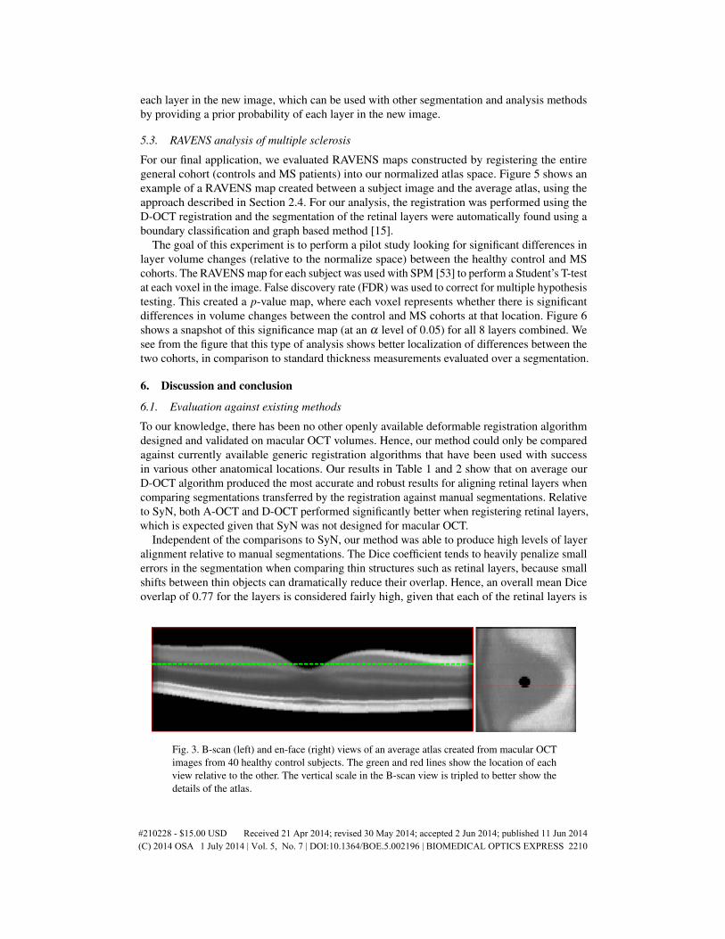
The 40 healthy control images in the general cohort were used to construct an average atlasfollowing the approach referenced in Section 2.3. Two iterations of the average atlas adjustmentwas applied in the atlas construction. Figure 3 shows two views of this average atlas. In thefollowing sections, this atlas is used as the target image for moving each subject into thenormalized space.

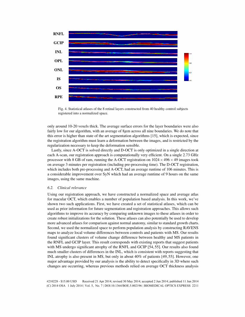
5.2. Statistical atlas

One useful application of a normalized macular OCT space is the ability to construct a statisticalrepresentation of spatial locations of retinal layers in the macula. By moving the retinal layersegmentations for each healthy control in the general cohort into this common space, we canempirically estimate the probability of a voxel belonging to a particular layer. Figure 4 showseach layer in a statistical atlas computed in this manner. Since everything is calculated in theaverage atlas space, the probabilities correspond spatially with the average atlas. Hence, if theaverage atlas is registered to a new image (or vice-verse), then the statistical atlas can be directlycarried over using the same deformation. This provides a statistical estimate of the location of


each layer in the new image, which can be used with other segmentation and analysis methodsby providing a prior probability of each layer in the new image.

5.3. RAVENS analysis of multiple sclerosis

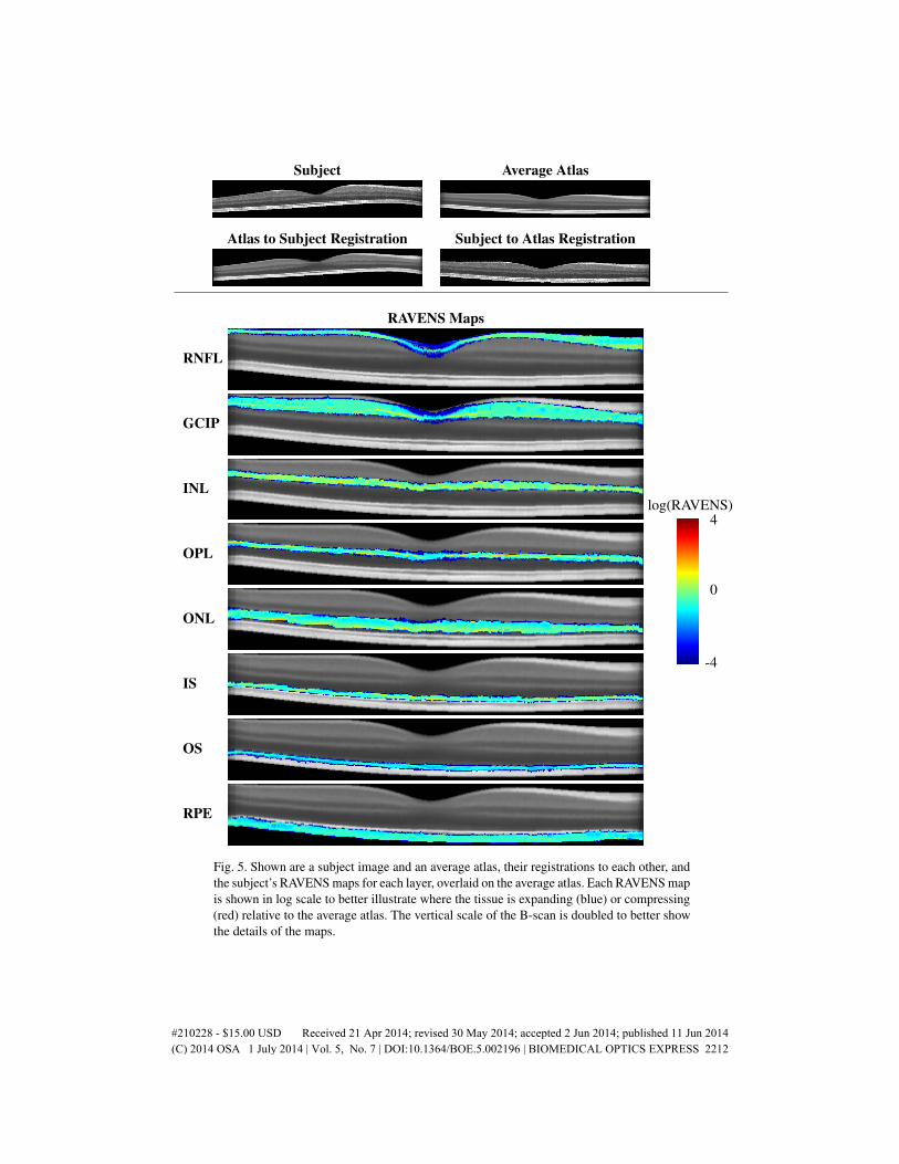
For our final application, we evaluated RAVENS maps constructed by registering the entiregeneral cohort (controls and MS patients) into our normalized atlas space. Figure 5 shows anexample of a RAVENS map created between a subject image and the average atlas, using theapproach described in Section 2.4. For our analysis, the registration was performed using theD-OCT registration and the segmentation of the retinal layers were automatically found using aboundary classification and graph based method [15].

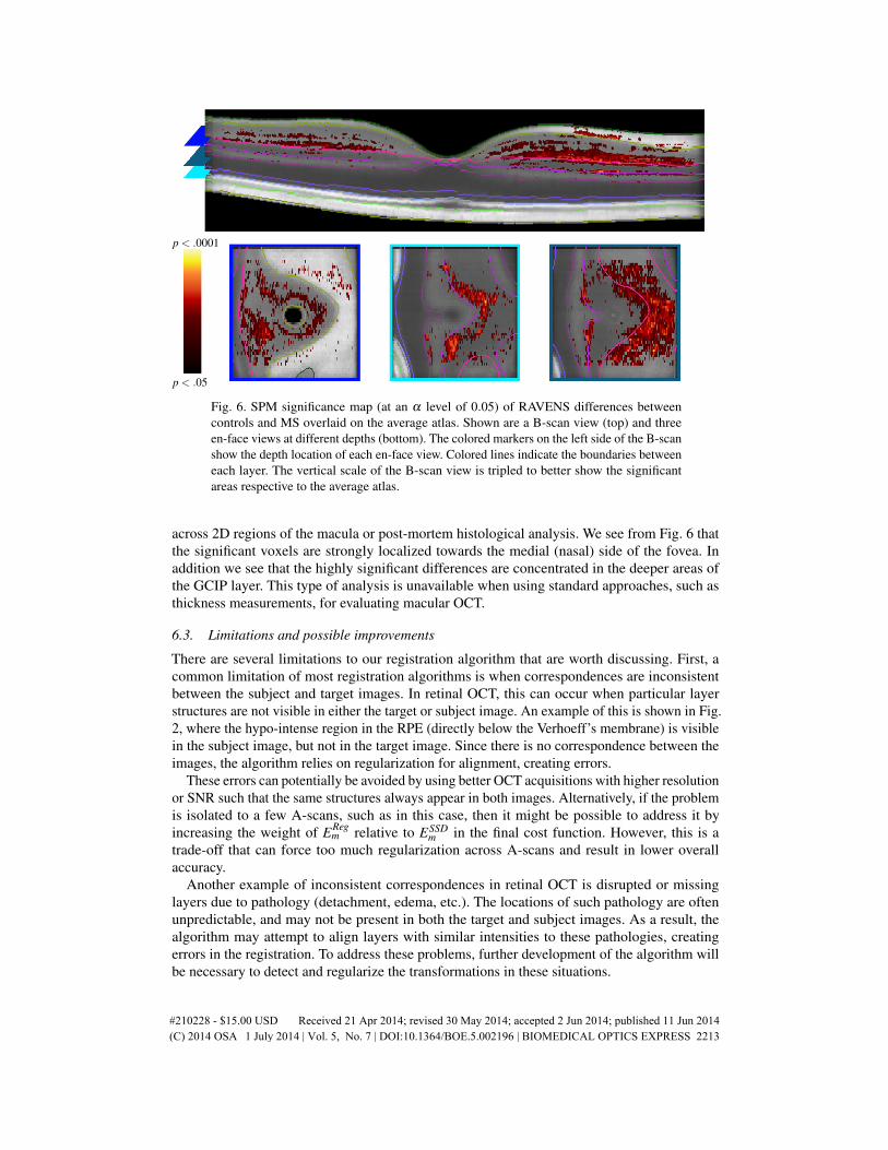
The goal of this experiment is to perform a pilot study looking for significant differences inlayer volume changes (relative to the normalize space) between the healthy control and MScohorts. The RAVENS map for each subject was used with SPM [53] to perform a Student’s T-testat each voxel in the image. False discovery rate (FDR) was used to correct for multiple hypothesistesting. This created a p-value map, where each voxel represents whether there is significantdifferences in volume changes between the control and MS cohorts at that location. Figure 6shows a snapshot of this significance map (at an α level of 0.05) for all 8 layers combined. Wesee from the figure that this type of analysis shows better localization of differences between thetwo cohorts, in comparison to standard thickness measurements evaluated over a segmentation.

6. Discussion and conclusion

6.1. Evaluation against existing methods

To our knowledge, there has been no other openly available deformable registration algorithmdesigned and validated on macular OCT volumes. Hence, our method could only be comparedagainst currently available generic registration algorithms that have been used with successin various other anatomical locations. Our results in Table 1 and 2 show that on average ourD-OCT algorithm produced the most accurate and robust results for aligning retinal layers whencomparing segmentations transferred by the registration against manual segmentations. Relativeto SyN, both A-OCT and D-OCT performed significantly better when registering retinal layers,which is expected given that SyN was not designed for macular OCT.

Independent of the comparisons to SyN, our method was able to produce high levels of layeralignment relative to manual segmentations. The Dice coefficient tends to heavily penalize smallerrors in the segmentation when comparing thin structures such as retinal layers, because smallshifts between thin objects can dramatically reduce their overlap. Hence, an overall mean Diceoverlap of 0.77 for the layers is considered fairly high, given that each of the retinal layers is

Fig. 3. B-scan (left) and en-face (right) views of an average atlas created from macular OCTimages from 40 healthy control subjects. The green and red lines show the location of eachview relative to the other. The vertical scale in the B-scan view is tripled to better show thedetails of the atlas.


RNFL

GCIP

INL

OPL

ONL

IS

OS

RPE

Fig. 4. Statistical atlases of the 8 retinal layers constructed from 40 healthy control subjectsregistered into a normalized space.

only around 10-20 voxels thick. The average surface errors for the layer boundaries were alsofairly low for our algorithm, with an average of 8µm across all nine boundaries. We do note thatthis error is higher than state of the art segmentation algorithms [15], which is expected, sincethe registration algorithm must learn a deformation between the images, and is restricted by theregularization necessary to keep the deformation sensible.

Lastly, since A-OCT is solved directly and D-OCT is only optimized in a single direction ateach A-scan, our registration approach is computationally very efficient. On a single 2.73 GHzprocessor with 8 GB of ram, running the A-OCT registration on 1024×496×49 images tookon average 3 minutes per registration (including pre-processing time). The D-OCT registration,which includes both pre-processing and A-OCT, had an average runtime of 106 minutes. This isa considerable improvement over SyN which had an average runtime of 9 hours on the sameimages, using the same machine.

6.2. Clinical relevance

Using our registration approach, we have constructed a normalized space and average atlasfor macular OCT, which enables a number of population based analysis. In this work, we’veshown two such applications. First, we have created a set of statistical atlases, which can beused as prior information for future segmentation and registration approaches. This allows suchalgorithms to improve its accuracy by comparing unknown images to these atlases in order tocreate robust initializations for the solution. These atlases can also potentially be used to developmore advanced atlases for comparison against normal anatomy, similar to standard growth charts.Second, we used the normalized space to perform population analysis by constructing RAVENSmaps to analyze local volume differences between controls and patients with MS. Our resultsfound significant clusters of volume change difference between healthy and MS patients inthe RNFL and GCIP layer. This result corresponds with existing reports that suggest patientswith MS undergo significant atrophy of the RNFL and GCIP [54, 55]. Our results also foundmuch smaller clusters of differences in the INL, which is consistent with reports suggesting thatINL atrophy is also present in MS, but only in about 40% of patients [49, 55]. However, onemajor advantage provided by our analysis is the ability to detect specifically in 3D where suchchanges are occurring, whereas previous methods relied on average OCT thickness analysis


Subject Average Atlas

Atlas to Subject Registration Subject to Atlas Registration

RAVENS Maps

RNFL

GCIP

INL

OPL

ONL

IS

OS

RPE

log(RAVENS)

-4

0

4

Fig. 5. Shown are a subject image and an average atlas, their registrations to each other, andthe subject’s RAVENS maps for each layer, overlaid on the average atlas. Each RAVENS mapis shown in log scale to better illustrate where the tissue is expanding (blue) or compressing(red) relative to the average atlas. The vertical scale of the B-scan is doubled to better showthe details of the maps.


p < .0001

p < .05

Fig. 6. SPM significance map (at an α level of 0.05) of RAVENS differences betweencontrols and MS overlaid on the average atlas. Shown are a B-scan view (top) and threeen-face views at different depths (bottom). The colored markers on the left side of the B-scanshow the depth location of each en-face view. Colored lines indicate the boundaries betweeneach layer. The vertical scale of the B-scan view is tripled to better show the significantareas respective to the average atlas.

across 2D regions of the macula or post-mortem histological analysis. We see from Fig. 6 thatthe significant voxels are strongly localized towards the medial (nasal) side of the fovea. Inaddition we see that the highly significant differences are concentrated in the deeper areas ofthe GCIP layer. This type of analysis is unavailable when using standard approaches, such asthickness measurements, for evaluating macular OCT.

6.3. Limitations and possible improvements

There are several limitations to our registration algorithm that are worth discussing. First, acommon limitation of most registration algorithms is when correspondences are inconsistentbetween the subject and target images. In retinal OCT, this can occur when particular layerstructures are not visible in either the target or subject image. An example of this is shown in Fig.2, where the hypo-intense region in the RPE (directly below the Verhoeff’s membrane) is visiblein the subject image, but not in the target image. Since there is no correspondence between theimages, the algorithm relies on regularization for alignment, creating errors.

These errors can potentially be avoided by using better OCT acquisitions with higher resolutionor SNR such that the same structures always appear in both images. Alternatively, if the problemis isolated to a few A-scans, such as in this case, then it might be possible to address it byincreasing the weight of EReg

m relative to ESSDm in the final cost function. However, this is a

trade-off that can force too much regularization across A-scans and result in lower overallaccuracy.

Another example of inconsistent correspondences in retinal OCT is disrupted or missinglayers due to pathology (detachment, edema, etc.). The locations of such pathology are oftenunpredictable, and may not be present in both the target and subject images. As a result, thealgorithm may attempt to align layers with similar intensities to these pathologies, creatingerrors in the registration. To address these problems, further development of the algorithm willbe necessary to detect and regularize the transformations in these situations.


Second, data limitations can directly affect the performance of the algorithm. Due to the sparsesampling of the B-scans in our Spectralis data, we are limited by the type of regularization andinterpolation allowed in the algorithm. Given data with higher resolutions and denser sampling,we can potentially improve the accuracy of the registration and provide better acuity in the typesof analysis we have demonstrated.

Third, errors during the data acquisition can affect the accuracy of the registration. Oneexample of this is the appearance of a rotation of the retina, often caused by the OCT scan notbeing centered on the pupil during the acquisition [56]. When the retina is tilted in the OCT, ourdiscrete translation of the A-scans becomes a less valid model for rigidly aligning the macula,which lowers our registration accuracy. In general, our algorithm cannot correct for this rotation,because rotating the OCT would cause the z-axis in the OCT to no longer represent the A-scans.This would make it difficult to justify any transformations along this axis, since the size ofeach voxel along the axis would now depend on the fan-beam separation, which depends on thecornea of the subject being imaged. Care must be taken to use data that is properly centered tominimize these errors.

Fourth, intensity inhomogeneity can still be a problem for the algorithm after intensitynormalization, where shifts in intensity can be seen in the OCT even after preprocessing. Onepotential improvement to address this is to use a similarity metric that is more robust to intensityvariabilities. Our preliminary results suggest that the cross-correlation measure may be a goodreplacement for SSD in future versions of the algorithm.

Lastly, since the detected ILM and BrM locations are used in the affine registration step,errors in their detection can cause poor initialization for the deformable registration step. Whilethis would not be detrimental to the algorithm, it does mean the deformable registration wouldneed to move the boundaries larger distances to find the correct alignment. This might causethe optimization to get caught in a local minima, resulting in errors in the final registration.Although the retinal mask is generally found very accurately and robustly in our experiments,certain pathology can make these boundaries difficult to detect. In such cases, the boundarydetection algorithm may need to be modified.

6.4. Conclusion

We have presented both an affine and deformable registration method designed specifically forOCT images of the macula, which respect the acquisition physics of the imaging modality. Ourvalidation using manual segmentations shows that our algorithm is considerably more accurateand robust for aligning retinal layers than existing generic registration algorithms. Our methodopens up a number of applications for analysis of OCT that were previously not available. Wehave demonstrated three such examples through the creation of an average atlas, a statistical atlas,and a pilot study of local volume changes in the macula of healthy controls and MS patients.However, these are but a small example of the existing methods and techniques that utilizedeformable registration and normalized spaces to perform population based analysis of healthand disease. The software for our OCT registration algorithm and atlas construction approachcan be freely downloaded as modules for the Java Image Science Toolkit (JIST) [57] softwarepackage at https://www.nitrc.org/projects/toads-cruise/.

Acknowledgments

This work was supported by the NIH/NEI under grant R21-EY022150, NIH/NINDS R01-NS082347 and the Intramural Research Program of NINDS.


Documents

Analysis of macular OCT images using deformable registration · Analysis of macular OCT images using deformable registration ... M. Hauser, E. S. Sotirchos, P. A. Calabresi, H. S