NREL is a national laboratory of the U.S. Department of Energy, Office of Energy Efficiency & Renewable Energy, operated by the Alliance for Sustainable Energy, LLC.

Contract No. DE-AC36-08GO28308

Analysis of High-Penetration Levels of Photovoltaics into the Distribution Grid on Oahu, Hawaii Detailed Analysis of HECO Feeder WF1 Dr. Emma Stewart, James MacPherson, and Slavko Vasilic BEW Engineering, A DNV Company San Ramon, California

Dr. Dora Nakafuji and Thomas Aukai Hawaiian Electric Company (HECO) Honolulu, Hawaii

NREL Technical Monitor: Jamie Keller

Subcontract Report NREL/SR-5500-54494 May 2013

NREL is a national laboratory of the U.S. Department of Energy, Office of Energy Efficiency & Renewable Energy, operated by the Alliance for Sustainable Energy, LLC.

National Renewable Energy Laboratory 15013 Denver West Parkway Golden, Colorado 80401 303-275-3000 • www.nrel.gov

Contract No. DE-AC36-08GO28308

Analysis of High-Penetration Levels of Photovoltaics into the Distribution Grid on Oahu, Hawaii Detailed Analysis of HECO Feeder WF1 Dr. Emma Stewart, James MacPherson, and Slavko Vasilic BEW Engineering, A DNV Company San Ramon, California

Dr. Dora Nakafuji and Thomas Aukai Hawaiian Electric Company (HECO) Honolulu, Hawaii

NREL Technical Monitor: Jamie Keller Prepared under Subcontract No. LXL-040281-01

Subcontract Report NREL/SR-5500-54494 May 2013

This publication received minimal editorial review at NREL.

NOTICE

This report was prepared as an account of work sponsored by an agency of the United States government. Neither the United States government nor any agency thereof, nor any of their employees, makes any warranty, express or implied, or assumes any legal liability or responsibility for the accuracy, completeness, or usefulness of any information, apparatus, product, or process disclosed, or represents that its use would not infringe privately owned rights. Reference herein to any specific commercial product, process, or service by trade name, trademark, manufacturer, or otherwise does not necessarily constitute or imply its endorsement, recommendation, or favoring by the United States government or any agency thereof. The views and opinions of authors expressed herein do not necessarily state or reflect those of the United States government or any agency thereof.

Available electronically at http://www.osti.gov/bridge

Available for a processing fee to U.S. Department of Energy and its contractors, in paper, from:

U.S. Department of Energy Office of Scientific and Technical Information P.O. Box 62 Oak Ridge, TN 37831-0062 phone: 865.576.8401 fax: 865.576.5728 email: mailto:reports@adonis.osti.gov

Available for sale to the public, in paper, from:

U.S. Department of Commerce National Technical Information Service 5285 Port Royal Road Springfield, VA 22161 phone: 800.553.6847 fax: 703.605.6900 email: orders@ntis.fedworld.gov online ordering: http://www.ntis.gov/help/ordermethods.aspx

Cover Photos: (left to right) PIX 16416, PIX 17423, PIX 16560, PIX 17613, PIX 17436, PIX 17721

Printed on paper containing at least 50% wastepaper, including 10% post consumer waste.

iii

Authors BEW Engineering, A DNV Company Prepared By: Dr. Emma Stewart, Senior Engineer, Power Systems James MacPherson, Engineer, Power Systems Slavko Vasilic, Senior Engineer, Power Systems

Verified By: Billy Quach, Senior Engineer, Power Systems Project Manager: Ron Davis, Director of Transmission and Distribution

Hawaii Electric Company (HECO) Dr. Dora Nakafuji, Director of Renewable Energy Planning Thomas Aukai, Renewable Energy Planning Engineer

Abstract Renewable generation is growing at a rapid rate due to the incentives available and the aggressive renewable portfolio standard (RPS) targets implemented by state governments. Distributed generation in particular is seeing the fastest growth among renewable energy projects, and is directly related to the incentives. Hawaii has the highest electricity costs in the country due to the high percentage of oil burning steam generation, and therefore has some of the highest penetration of distributed PV in the nation. The High Penetration PV (HiP-PV) project on Oahu aims to understand the effects of high penetration PV on the distribution level, to identify penetration levels creating disturbances on the circuit, and to offer mitigating solutions based on model results. Power flow models are validated using data collected from solar resources and load monitors deployed throughout the circuit. Existing interconnection methods and standards such as IEEE 1547, Hawaii Rule 14H and California Rule 21 are evaluated in these emerging high penetration scenarios. A key finding is a shift in the level of detail to be considered and moving away from steady-state peak time analysis towards dynamic and time varying simulations. Each level of normal interconnection study is evaluated and enhanced to a new level of detail, allowing full understanding of each issue.

iv

Acronyms BEW BEW Engineering DG Distributed Generation HECO Hawaii Electric Company GIS Geographical Information Systems LTC Load Tap Changer (located on Substation Transformer) LDC Line Drop Compensation (enabled on LTC normally) NREL National Renewable Energy Laboratory OPS Operations at HECO PSLF Transmission power flow simulation model developed by General Electric PSS/E Transmission power flow simulation model developed by Siemens PV Photovoltaic RPS Renewable Portfolio Standard SCADA Supervisory Control and Data Acquisition SLACA Substation Load and Capacity Analysis SynerGEE Electric– Distribution simulation model developed by GL-Group Confidentiality Statement This report was prepared by BEW Engineering, a subsidiary of Det Norske Veritas (DNV), as an account of work undertaken under the authorization of Hawaii Electric Company (HECO). Material in this report is considered confidential by BEW Engineering and HECO. No part of this report is to be released to any third party (outside of BEW and HECO), without express written permission from both HECO and BEW. However, it is assumed that, after approval from HECO, this document will be published as a subcontract report by the National Renewable Energy Laboratory (NREL).

Acknowledgements This work is jointly funded under the DOE NREL Hi-Pen Initiative, California Public Utilities Commissions, California Solar Initiative RD&D project, with funds also provided by Sacramento Municipal Utilities District and Hawaiian Electric Company. The authors also gratefully acknowledge the contribution of Elaine Sison-Lebrilla of Sacramento Municipal Utilities District.

v

Contents Authors ........................................................................................................................................................ iii Abstract ....................................................................................................................................................... iii Acronyms .................................................................................................................................................... iv Confidentiality Statement .......................................................................................................................... iv Acknowledgements ................................................................................................................................... iv List of Figures ............................................................................................................................................ vi List of Tables .............................................................................................................................................. vi 1 Introduction ........................................................................................................................................... 1

1.1 Feeder Selection ............................................................................................................................... 2 1.2 Changing Perception of Technical Barriers to High Renewable Penetrations ................................. 2

2 Summarizing New Conditions for Interconnect Studies .................................................................. 3 3 Distribution Feeder Modeling .............................................................................................................. 5

3.1 Analysis Assumptions ...................................................................................................................... 6 4 Selecting Analysis Focal Points from Measured Data...................................................................... 6 5 Load Flow and Voltage Trends ......................................................................................................... 12

5.1 Steady State Voltage Trends on WF1 ............................................................................................ 13 5.2 Thermal Limitations....................................................................................................................... 14 5.3 Backfeed ........................................................................................................................................ 15

6 Tap Changer Cycling .......................................................................................................................... 17 7 Protection and Short Circuit Analysis .............................................................................................. 20 8 Dynamic Studies ................................................................................................................................. 21

8.1 N-1 Dynamic Analysis ................................................................................................................... 22 8.2 All PV Trip Conditions .................................................................................................................. 24 8.3 Flicker Study .................................................................................................................................. 26

9 Conclusions and Future Work .......................................................................................................... 31 9.1 Limitations Specific to WF1 .......................................................................................................... 31 9.2 Comparison to Normal Standards and Interconnect Processes ...................................................... 32 9.3 Types and Levels of Analysis Recommended Based on Feeder Study ......................................... 33 9.4 Future Work ................................................................................................................................... 34

10 References .......................................................................................................................................... 35

vi

List of Figures Figure 1: Simplified one-line diagram of W1 Substation, and WF1 Feeder .......................................... 2 Figure 2: Feeder WF1 load and irradiance monitor locations ................................................................ 7 Figure 3: Change in tap position during week of April 16 - 21 ............................................................... 9 Figure 4: Real power measurement week of April 16 - 21 ...................................................................... 9 Figure 5: 3 Individual & average irradiance sensor measurements April 17; average irradiance

April 19 ................................................................................................................................................. 10 Figure 6: 3 Average irradiance sensor measurements April 1 ............................................................. 10 Figure 7: Binning of tap changer counts for each month above a mean of 5 .................................... 11 Figure 8: Number of events, of 1-second variability in irradiance measurement, plotted monthly . 12 Figure 9: Voltage trends in minimum daytime load conditions on WF1 with varying PV penetration

levels .................................................................................................................................................... 13 Figure 10: Load trend on feeder with and without PV at peak and maximum load ........................... 14 Figure 11: Minimum measured day, plotted with measured irradiance data and scaled for April 9 to

show potential backfeed levels ......................................................................................................... 16 Figure 12: Minimum measured day, with 1.6 MW of PV generating on April 9 results in backfeed in

the middle of the day .......................................................................................................................... 17 Figure 13: Sunny and cloudy day for tap changer cycling analysis over 24 hours ........................... 18 Figure 14: Tap changer position movement with existing PV on a sunny and cloudy day on WF1 19 Figure 15: Tap changer position movement with 60% PV on a sunny and cloudy day on WF1 ...... 19 Figure 16: Tap changer position movement with 100% PV on a sunny and cloudy day on WF1 .... 19 Figure 17: System frequency variation during an N-1 conventional generator trip with no PV (blue),

Hi-PV on the WF1 Feeder only (red), and Hi-PV in the W1 area (green) ....................................... 23 Figure 18: 12 kV bus voltage variation with no PV (blue), and Hi-PV on WF1 (red) during an N-1

conventional generator trip ............................................................................................................... 23 Figure 19: 12 kV bus voltage variation with no PV (blue), Hi-PV on WF1 (red), and very Hi-PV on

WF1 (green) during an all PV trip scenario such as an anti-islanding event ............................... 24 Figure 20: 12 kV bus voltage variation Hi-PV on WF1 (blue) and Hi-PV in W1 area (red) during an

All PV trip scenario such as an anti-islanding event ...................................................................... 25 Figure 21: 46 kV bus voltage variation Hi PV on WF1 (blue) and Hi-PV in W1 area (red) during an

All PV trip scenario such as an anti-islanding event ...................................................................... 26 Figure 22: Irradiance plots of two representative variable irradiance days across 5 sensors from

the Airport irradiance grid for input to the flicker analysis ............................................................ 28 Figure 23: 12 kV bus voltage variation for the 5 highly variable irradiance days input to the

dynamic inverter model connected to WF1 ..................................................................................... 29 Figure 24: 12 kV bus voltage variation for the most variable voltage response ................................ 29 Figure 25: GE flicker curve [4] ................................................................................................................. 30 Figure 26: Comparison of 12 kV bus voltage for an instantaneous power output drop and a

variable irradiance change ................................................................................................................ 30 Figure 27: Types of analysis and when to consider during the interconnect process ..................... 33

List of Tables Table 1: Enhancements to the typical PV interconnect process completed for WF1 ......................... 4

1

1 Introduction The HiP-PV [1], implemented in June 2010, addresses common issues between the Sacramento Municipal Utility District (SMUD) and HECO. Both utilities adopted aggressive renewable energy targets with SMUD targeting 37% by 2020 and HECO targeting 40% by 2030 for the three Hawaiian utilities. In conjunction with HiP-PV, NREL funded a collaborative effort together with HECO and BEW Engineering (BEW). These studies aim to characterize impacts of high PV penetrations on different types of distribution feeders and improve future interconnection processes.

This report pertains to specific analysis on feeder WF1 that was selected because of the existing feeder PV penetration level, diversity of customer types, and available solar sensor locations [2]. Study of individual feeder impacts provides insight to the potential barriers and issues restricting higher PV penetrations across both the Hawaiian and Sacramento utility areas. Commonly followed distributed generation (DG) standards such as IEEE 1547 [3] and IEEE 519 [4] are open to interpretation through the interconnection process. In-depth feeder analysis helps standardize and clarify the detail of measured data and analysis required. Lessons learned to date include:

• Availability of measured data is key to fully understanding impacts and sustainable development

• Software integration is essential for maintaining and growing PV portfolios

• Utilities must prepare for high penetrations of variable resources

• Legacy or aging distribution equipment, such as load tap changers, are particularly impacted by variability of high PV penetrations

• Utilities must plan for upgrades and operational changes ahead of time, with informed and validated analysis

• All stakeholders (i.e., operations, transmission and distribution planning, government agencies and developers) must find common ground for continued sustainable development.

The traditional distribution system is designed to deliver power from generator to customer load, and therefore all the control and protection equipment on the system are designed to move generation from system to load. Now, local load centers can generate sufficient power to service the local needs.

Under feed-in-tariff (FIT) programs, eligible renewable energy projects can produce power to sell back to utilities. As more of the local, distributed generation is expected to come from variable, nondispatchable PV resources, utilities like HECO need to better plan contributions from nondispatchable local generation. Visibility and monitoring of these nondispatchable resources is an essential piece of the future planning process.

2

1.1 Feeder Selection Feeder WF1 is selected for the first portion of the HECO/SMUD HiP-PV penetration study. WF1 has a mix of residential and commercial customers distributed along the length of the feeder, allowing a wide range of PV installation types to be investigated. At the time of selection, WF1 had the highest existing penetration of PV installed of more than 20% and has a high number of available sensor locations and GIS data available. The WF1 12 kV feeder is connected to W1 transformer from the substation 46 kV line. Figure 1 shows a simplified one-line diagram of the circuit. The W1 area, used later in the analysis, is defined as the Substation, and all other distribution substations fed from the same 46 kV line.

Figure 1: Simplified one-line diagram of W1 Substation, and WF1 Feeder

WF1 has 26% PV (of the feeder non-coincident peak demand) penetration, including 3 large PV locations at 500 kW, 218 kW, and 42 kW. Non-coincident peak demand indicates the single peak time for the feeder WF1 occurring at only one time during the year (originally selected as 2010 in this case). The non-coincident feeder peak does not always occur at the same time as system peak. There is a 3.6 MVAr capacitor on WF1 located in the substation that is fixed and normally on. There are no line voltage regulators on WF1.

1.2 Changing Perception of Technical Barriers to High Renewable Penetrations

There are two approaches to using the distribution power flow simulation models and PV profiles. These are proactive and reactive. The proactive approach is the advanced study and planning of the distribution grid to determine where the potential problems could occur, the corrective action necessary, and the PV penetration level that creates the problem. The reactive approach is the study of each individual PV installation as it becomes commercial or into the queue.

Load Pocket

W1 XFRMR 46kV:12kV

~ 40-kW Distributed Residential PV

~760-kW Large PV

NC

3.6-MVAr

CB 1420 WF1

WF4

WF3

CB 1441 WF2

W2 XFRMR 46kV:12kV

3

As identified in recent federal stimulus proposals and projects being completed by BEW on high penetration impacts of PV on distribution systems [1], lack of observability (meaning ability to observe) and commercial tools to control high penetration of variable distributed generation are not only a Hawaii issue but a national concern. Individually, a residential-scale PV system does not impact system reliability. However, aggregated in large concentrations on a distribution circuit, these may pose reliability and protection concerns that warrant further investigation.

An example of the change in perception of interconnect requirements is voltage flicker caused by distributed generation. This change in analysis technique and perception is detailed in Section 8.3, described here as an example of the feeder results. Voltage flicker is widely discussed during System Impact Studies or Interconnection Studies by the control area operator or the electric utility. Misrepresentation of voltage flicker can often delay or create barriers for renewable energy projects' entry into the market. The simplest voltage flicker analysis for PV generation is based on perceived instantaneous irradiance dips of approximately 80% to 90%. These instantaneous post-transient simulations often do not account for transient stability of inverters and time varying generation output.

With emerging distributed PV resources, especially at high feeder and nodal penetration levels, the instantaneous power output methodology for flicker analysis may be too restrictive and an alternative approach such as using realistic, time series irradiance profiles may be needed to accurately capture PV impact. This is a future goal of the HiP-PV studies, as a single feeder analysis cannot quantify data collection goals for all feeders, but provides guidance for future studies to build on.

Hawaii Legislation Rule 14H and California Rule 21 define a 15% DG penetration level as a trigger for detailed interconnect studies. Historically, the 15% screen for PV penetration was selected based on probability of islanding. It was an administrative screen based on a 2 times safety factor with assumed 30% minimum load. Within the Hawaiian utilities, many distribution feeders exceed this ‘rule of thumb’ penetration filter. Utilities have limited observability to demand data at the distribution system level. If data is available, it is often on a longer time scale than required, such as 15 minute time steps versus 1 to 30 seconds. 15-minute increments of data can inform generation dispatch, but there is no visibility of irradiance fluctuations at this scale.

The HiP-PV project provides this observability through installation of high fidelity monitoring devices for both the distribution feeder load level and co-located irradiance measurement devices. The benefits of this are two-fold: (1) allow HECO to understand what data must be collected and at what fidelity to accurately quantify High PV impacts; and (2) allow validation of modeling techniques for future analyses.

2 Summarizing New Conditions for Interconnect Studies

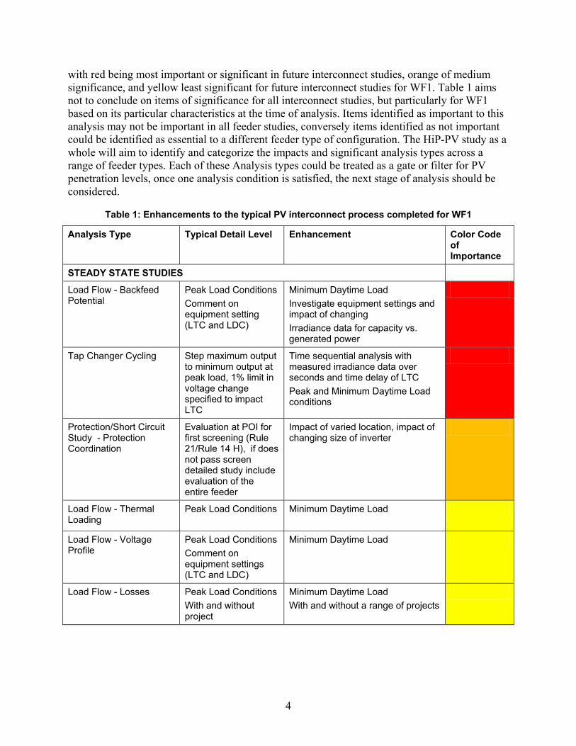
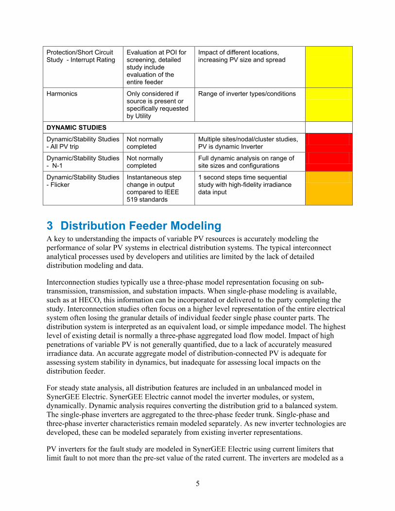
Analysis is performed to a level of detail often not considered necessary in many interconnect areas. The table below indicates normally considered issues during HECO and other utility interconnect studies. The last column details the enhanced process considered in this analysis. Coloring of Table 1 items indicates importance, defined based on the single WF1 feeder analysis,

4

with red being most important or significant in future interconnect studies, orange of medium significance, and yellow least significant for future interconnect studies for WF1. Table 1 aims not to conclude on items of significance for all interconnect studies, but particularly for WF1 based on its particular characteristics at the time of analysis. Items identified as important to this analysis may not be important in all feeder studies, conversely items identified as not important could be identified as essential to a different feeder type of configuration. The HiP-PV study as a whole will aim to identify and categorize the impacts and significant analysis types across a range of feeder types. Each of these Analysis types could be treated as a gate or filter for PV penetration levels, once one analysis condition is satisfied, the next stage of analysis should be considered.

Table 1: Enhancements to the typical PV interconnect process completed for WF1

Analysis Type Typical Detail Level Enhancement Color Code of Importance

STEADY STATE STUDIES

Load Flow - Backfeed Potential

Peak Load Conditions Comment on equipment setting (LTC and LDC)

Minimum Daytime Load Investigate equipment settings and impact of changing Irradiance data for capacity vs. generated power

Tap Changer Cycling Step maximum output to minimum output at peak load, 1% limit in voltage change specified to impact LTC

Time sequential analysis with measured irradiance data over seconds and time delay of LTC Peak and Minimum Daytime Load conditions

Protection/Short Circuit Study - Protection Coordination

Evaluation at POI for first screening (Rule 21/Rule 14 H), if does not pass screen detailed study include evaluation of the entire feeder

Impact of varied location, impact of changing size of inverter

Load Flow - Thermal Loading

Peak Load Conditions Minimum Daytime Load

Load Flow - Voltage Profile

Peak Load Conditions Comment on equipment settings (LTC and LDC)

Minimum Daytime Load

Load Flow - Losses Peak Load Conditions With and without project

Minimum Daytime Load With and without a range of projects

5

Protection/Short Circuit Study - Interrupt Rating

Evaluation at POI for screening, detailed study include evaluation of the entire feeder

Impact of different locations, increasing PV size and spread

Harmonics Only considered if source is present or specifically requested by Utility

Range of inverter types/conditions

DYNAMIC STUDIES

Dynamic/Stability Studies - All PV trip

Not normally completed

Multiple sites/nodal/cluster studies, PV is dynamic Inverter

Dynamic/Stability Studies - N-1

Not normally completed

Full dynamic analysis on range of site sizes and configurations

Dynamic/Stability Studies - Flicker

Instantaneous step change in output compared to IEEE 519 standards

1 second steps time sequential study with high-fidelity irradiance data input

3 Distribution Feeder Modeling A key to understanding the impacts of variable PV resources is accurately modeling the performance of solar PV systems in electrical distribution systems. The typical interconnect analytical processes used by developers and utilities are limited by the lack of detailed distribution modeling and data.

Interconnection studies typically use a three-phase model representation focusing on sub-transmission, transmission, and substation impacts. When single-phase modeling is available, such as at HECO, this information can be incorporated or delivered to the party completing the study. Interconnection studies often focus on a higher level representation of the entire electrical system often losing the granular details of individual feeder single phase counter parts. The distribution system is interpreted as an equivalent load, or simple impedance model. The highest level of existing detail is normally a three-phase aggregated load flow model. Impact of high penetrations of variable PV is not generally quantified, due to a lack of accurately measured irradiance data. An accurate aggregate model of distribution-connected PV is adequate for assessing system stability in dynamics, but inadequate for assessing local impacts on the distribution feeder.

For steady state analysis, all distribution features are included in an unbalanced model in SynerGEE Electric. SynerGEE Electric cannot model the inverter modules, or system, dynamically. Dynamic analysis requires converting the distribution grid to a balanced system. The single-phase inverters are aggregated to the three-phase feeder trunk. Single-phase and three-phase inverter characteristics remain modeled separately. As new inverter technologies are developed, these can be modeled separately from existing inverter representations.

PV inverters for the fault study are modeled in SynerGEE Electric using current limiters that limit fault to not more than the pre-set value of the rated current. The inverters are modeled as a

6

current source during a fault with a current rating at a range of 1.1 to 1.3 times the normal rated current of the PV inverter. In SynerGEE, the current source is created by using a feeder node for an ideal voltage source and a transformer impedance to convert to a current source. The magnitude of the current is a function of the transformer impedance, transformer kVA rating, and kV at the Point of Interconnection.

In dynamic studies, it is essential to represent the characteristics of all components deemed contributors to dynamic response, including PV inverters. In PSLF, the WF1 inverters are represented using a combination of standard dynamic generator models and user-developed models to represent specific control functions. The basic generator representation of a PV unit is replaced with the generic inverter- PV generator combination. Three separate PSLF models are required to accurately model one PV unit regardless of size or phase configuration, as shown below:

• gewtg (standard PSLF model)

• ewtgfc (standard PSLF model)

• epcmod (user-defined PSLF model).

3.1 Analysis Assumptions The steady state and dynamic study assumptions include:

• IEEE standards [3] state the inverter shall not control voltage at the point of interconnection therefore not considered throughout this analysis. Voltage is regulated by tap changers and capacitors

• Low voltage (customer supply side) is not modeled

• Highly distributed potential PV does not exceed the size of the distribution transformer at any particular load point

• PV generation cannot exceed the maximum line rating of this feeder

• Under and over frequency settings, and under/over voltage protection is set in the dynamic inverter model according to IEEE 1547 limits [3]

• Normal practice or indicators of problems for equipment, such as mean number of tap changer operations for a 24-hour period, are defined by historical information and monitored performance of equipment.

4 Selecting Analysis Focal Points from Measured Data

Previous to this analysis, there has been little collection and correlation of power monitor and irradiance data, particularly to the high fidelity considered here. Two types of data are collected from the W1 area; (1) high fidelity load monitor data from the W1 substation and a small amount (3 days) of high fidelity data from one large customer location; and (2) high-fidelity irradiance data from three locations on or nearby WF1. All data is time stamped and synchronized using

7

global positioning system (GPS) devices. Two groups of issues are selected for enhanced analysis based on the measured data:

1. Variability impacts on voltage regulation equipment

2. Load reduction and backfeed impacts.

The aim of high-fidelity data collection is to conduct further analysis on the impacts of high penetrations of PV on this feeder with a validated model. Irradiance and Power Monitor Data from W1 substation is collected from December 2010 to June 2011. Data continues to be collected up to the date of this report. Three days of data from the load side of the transformer at Large Customer 1 is collected. The aim of the data collection is to:

• Decouple effects of normal daily load patterns and PV generation impacts using measured data

• Validate feeder models

• Determine required data fidelity for investigating PV variability impacts on the distribution grid.

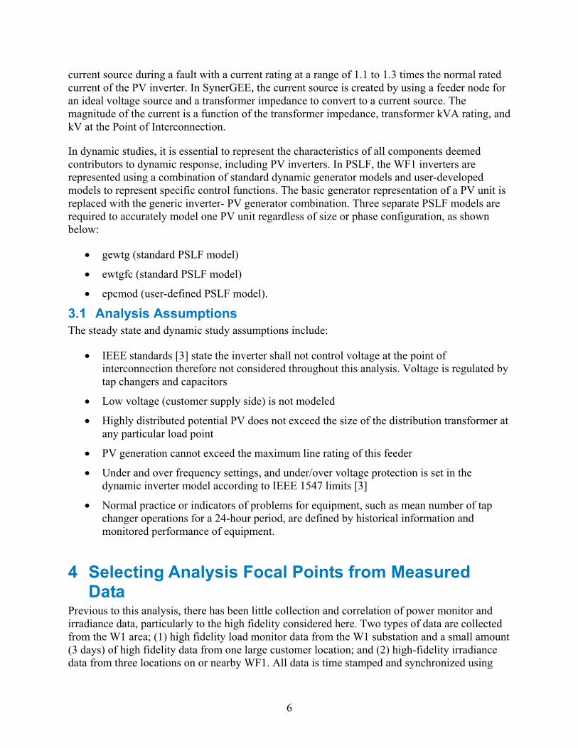
The monitored power locations, irradiance locations and existing PV locations are detailed below (Figure 2).

Figure 2: Feeder WF1 load and irradiance monitor locations

Model validation is performed initially to determine how accurate distribution models must be or currently are. The feeder load flow is validated over multiple time periods against voltage, current and tap changer positions. Errors are defined to be within 5% accuracy and this is deemed a successful validation. Accuracy standards for modeling are consistent with HECO

Large Customer 1 & Load Monitor Location

Irradiance Sensor 3 Location

Large Customer 2 & 3

Existing PV Site

Substation & Load Monitor Location Irradiance Sensor 1 Location

Irradiance Sensor 2 Location

8

design tolerances and standard industry practice (based on IEEE standards for transformer design tolerance) [5].

The interaction and coordination between LTC, capacitor, and inverter operations for increased PV penetration and varying operational scenarios are a concern of many system operators, but are not normally considered part of the interconnection study. This issue is generally not a problem for single distribution sites, but when a large cluster or node of sites experiences highly variable cloud cover, there could be increased tap changer operations and inverter tripping. The voltage and frequency impact of inverter tripping (anti-islanding for example) is therefore considered part of the enhanced dynamic analysis.

From the six months of measured data, ‘interesting’ days are selected where operation is deemed to be different from the perceived normal. For example, the mean number of tap changer operations greater than five is considered unusual (HECO operations definition); therefore all days with a count greater are extracted and compared to irradiance data and other operational information to determine the cause. Two primary reasons are considered for increased tap changer operations: Either PV irradiance variability or a utility feeder switching action. Without detailed measured plant output, the conclusions are not definitive, but a comparison of tap changer operations is presented and variable irradiance is identified as a preliminary reason for the increase.

Items defined as interesting from the measured data are:

• High voltage at the transformer

• Unbalanced voltages (+/- 3% [6])

• Large numbers of tap change operations (above mean)

• Rapid changes in power

• Other outstanding days.

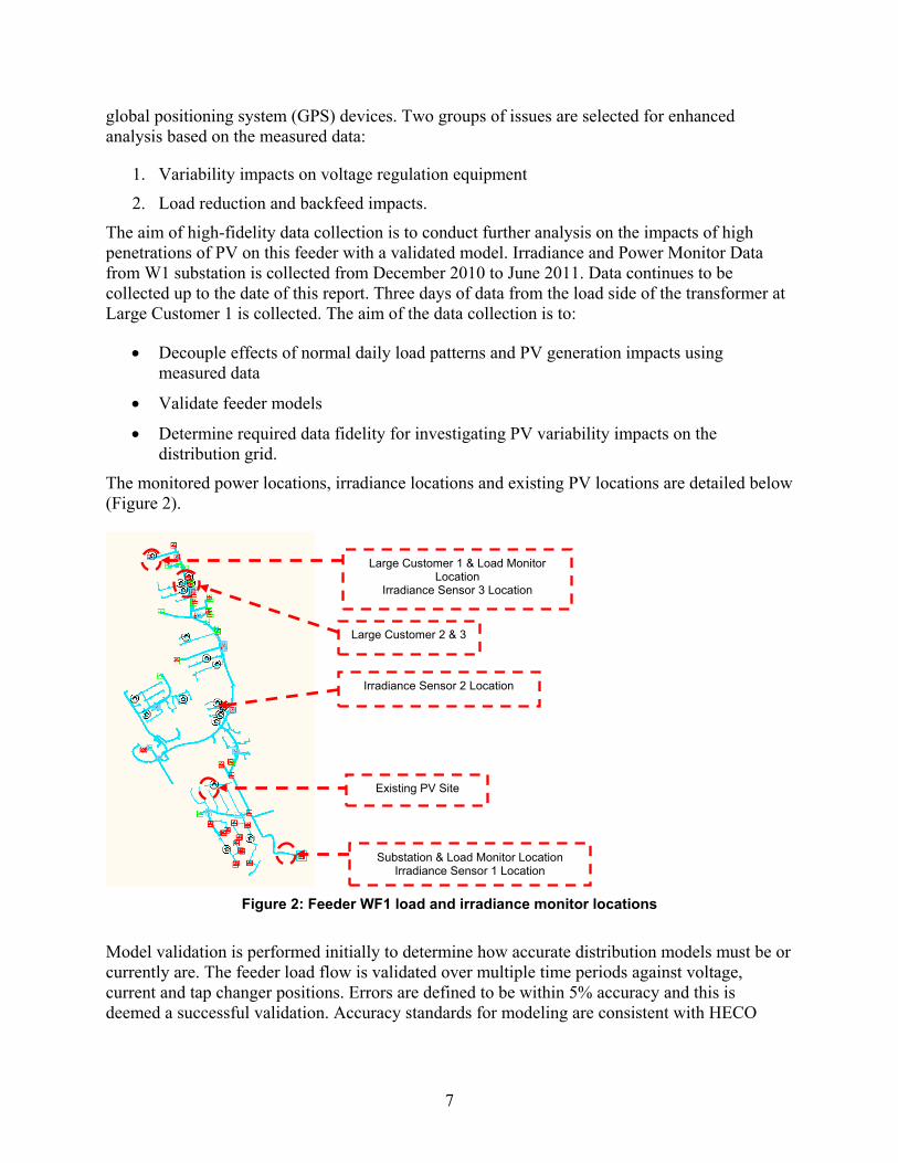
Tap position during a week in April is presented below (Figure 3), during which unusual numbers of tap change operations are recorded.

9

Figure 3: Change in tap position during week of April 16 - 21

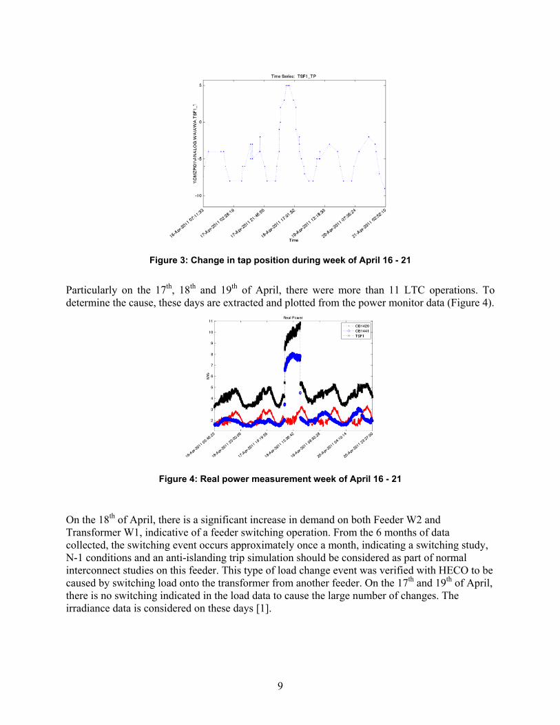
Particularly on the 17th, 18th and 19th of April, there were more than 11 LTC operations. To determine the cause, these days are extracted and plotted from the power monitor data (Figure 4).

Figure 4: Real power measurement week of April 16 - 21

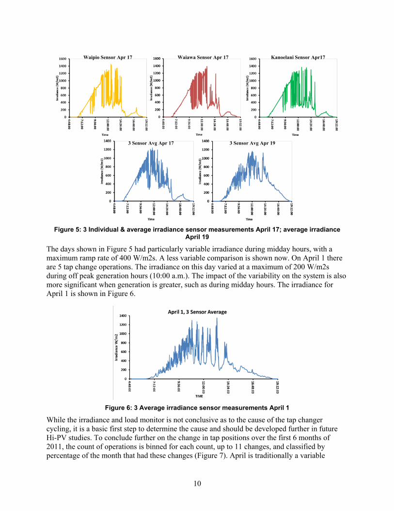
On the 18th of April, there is a significant increase in demand on both Feeder W2 and Transformer W1, indicative of a feeder switching operation. From the 6 months of data collected, the switching event occurs approximately once a month, indicating a switching study, N-1 conditions and an anti-islanding trip simulation should be considered as part of normal interconnect studies on this feeder. This type of load change event was verified with HECO to be caused by switching load onto the transformer from another feeder. On the 17th and 19th of April, there is no switching indicated in the load data to cause the large number of changes. The irradiance data is considered on these days [1].

10

Figure 5: 3 Individual & average irradiance sensor measurements April 17; average irradiance

April 19

The days shown in Figure 5 had particularly variable irradiance during midday hours, with a maximum ramp rate of 400 W/m2s. A less variable comparison is shown now. On April 1 there are 5 tap change operations. The irradiance on this day varied at a maximum of 200 W/m2s during off peak generation hours (10:00 a.m.). The impact of the variability on the system is also more significant when generation is greater, such as during midday hours. The irradiance for April 1 is shown in Figure 6.

Figure 6: 3 Average irradiance sensor measurements April 1

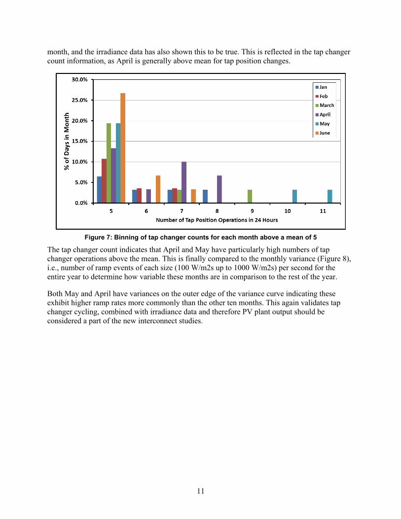
While the irradiance and load monitor is not conclusive as to the cause of the tap changer cycling, it is a basic first step to determine the cause and should be developed further in future Hi-PV studies. To conclude further on the change in tap positions over the first 6 months of 2011, the count of operations is binned for each count, up to 11 changes, and classified by percentage of the month that had these changes (Figure 7). April is traditionally a variable

Waipio Sensor Apr 17 Waiawa Sensor Apr 17 Kanoelani Sensor Apr17

3 Sensor Avg Apr 17 3 Sensor Avg Apr 19

11

month, and the irradiance data has also shown this to be true. This is reflected in the tap changer count information, as April is generally above mean for tap position changes.

Figure 7: Binning of tap changer counts for each month above a mean of 5

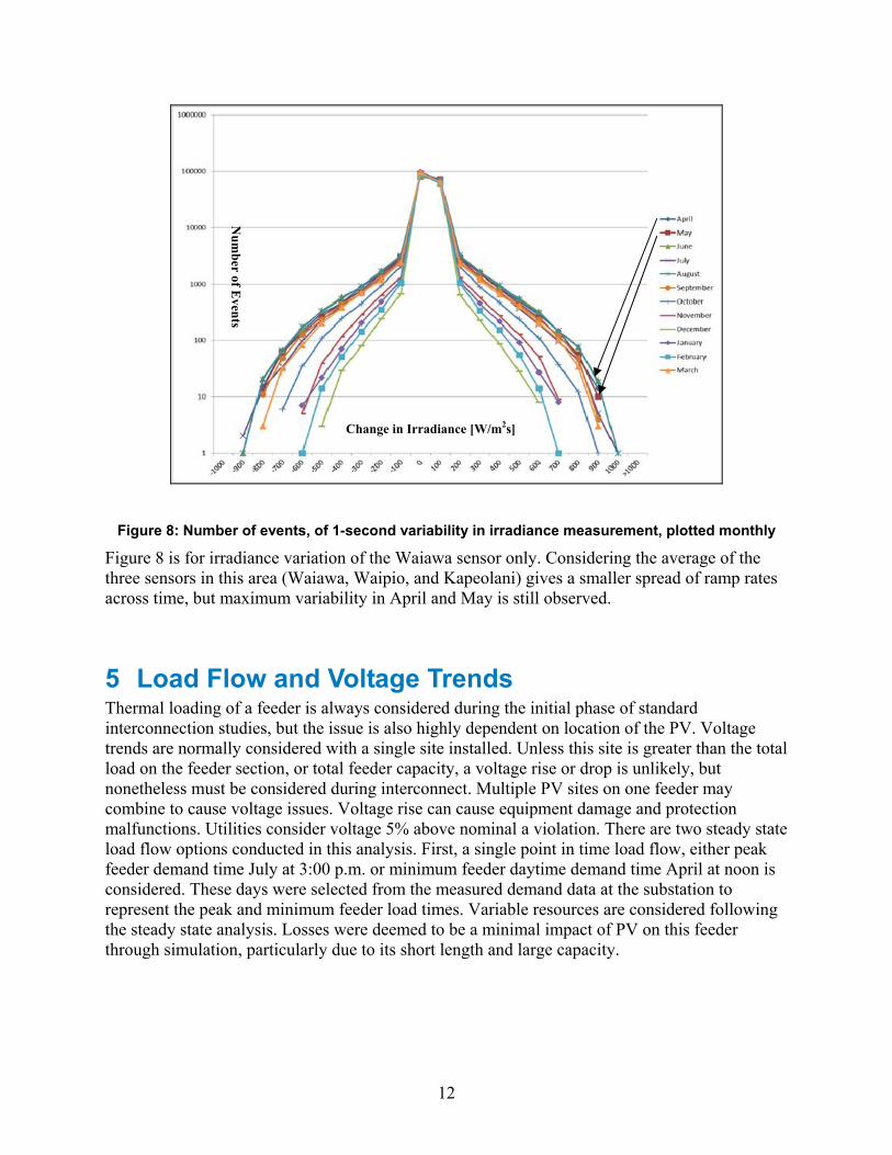
The tap changer count indicates that April and May have particularly high numbers of tap changer operations above the mean. This is finally compared to the monthly variance (Figure 8), i.e., number of ramp events of each size (100 W/m2s up to 1000 W/m2s) per second for the entire year to determine how variable these months are in comparison to the rest of the year.

Both May and April have variances on the outer edge of the variance curve indicating these exhibit higher ramp rates more commonly than the other ten months. This again validates tap changer cycling, combined with irradiance data and therefore PV plant output should be considered a part of the new interconnect studies.

12

Figure 8: Number of events, of 1-second variability in irradiance measurement, plotted monthly

Figure 8 is for irradiance variation of the Waiawa sensor only. Considering the average of the three sensors in this area (Waiawa, Waipio, and Kapeolani) gives a smaller spread of ramp rates across time, but maximum variability in April and May is still observed.

5 Load Flow and Voltage Trends Thermal loading of a feeder is always considered during the initial phase of standard interconnection studies, but the issue is also highly dependent on location of the PV. Voltage trends are normally considered with a single site installed. Unless this site is greater than the total load on the feeder section, or total feeder capacity, a voltage rise or drop is unlikely, but nonetheless must be considered during interconnect. Multiple PV sites on one feeder may combine to cause voltage issues. Voltage rise can cause equipment damage and protection malfunctions. Utilities consider voltage 5% above nominal a violation. There are two steady state load flow options conducted in this analysis. First, a single point in time load flow, either peak feeder demand time July at 3:00 p.m. or minimum feeder daytime demand time April at noon is considered. These days were selected from the measured demand data at the substation to represent the peak and minimum feeder load times. Variable resources are considered following the steady state analysis. Losses were deemed to be a minimal impact of PV on this feeder through simulation, particularly due to its short length and large capacity.

Change in Irradiance [W/m2s]

Num

ber of Events

13

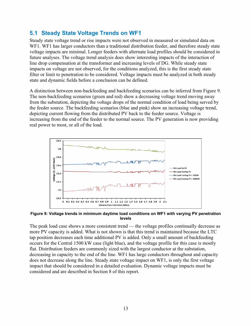
5.1 Steady State Voltage Trends on WF1 Steady state voltage trend or rise impacts were not observed in measured or simulated data on WF1. WF1 has larger conductors than a traditional distribution feeder, and therefore steady state voltage impacts are minimal. Longer feeders with alternate load profiles should be considered in future analyses. The voltage trend analysis does show interesting impacts of the interaction of line drop compensation at the transformer and increasing levels of DG. While steady state impacts on voltage are not observed, for the conditions analyzed, this is the first steady state filter or limit to penetration to be considered. Voltage impacts must be analyzed in both steady state and dynamic fields before a conclusion can be defined.

A distinction between non-backfeeding and backfeeding scenarios can be inferred from Figure 9. The non-backfeeding scenarios (green and red) show a decreasing voltage trend moving away from the substation, depicting the voltage drops of the normal condition of load being served by the feeder source. The backfeeding scenarios (blue and pink) show an increasing voltage trend, depicting current flowing from the distributed PV back to the feeder source. Voltage is increasing from the end of the feeder to the normal source. The PV generation is now providing real power to most, or all of the load.

Figure 9: Voltage trends in minimum daytime load conditions on WF1 with varying PV penetration

levels

The peak load case shows a more consistent trend — the voltage profiles continually decrease as more PV capacity is added. What is not shown is that this trend is maintained because the LTC tap position decreases each time additional PV is added. Only a small amount of backfeeding occurs for the Central 1500 kW case (light blue), and the voltage profile for this case is mostly flat. Distribution feeders are commonly sized with the largest conductor at the substation, decreasing in capacity to the end of the line. WF1 has large conductors throughout and capacity does not decrease along the line. Steady state voltage impact on WF1, is only the first voltage impact that should be considered in a detailed evaluation. Dynamic voltage impacts must be considered and are described in Section 8 of this report.

14

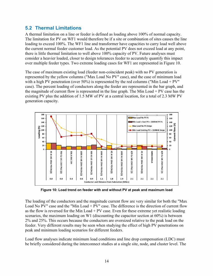
5.2 Thermal Limitations A thermal limitation on a line or feeder is defined as loading above 100% of normal capacity. The limitation for PV on WF1 would therefore be if a site or combination of sites causes the line loading to exceed 100%. The WF1 line and transformer have capacities to carry load well above the current normal feeder customer load. As the potential PV does not exceed load at any point, there is little thermal limitation to well above 100% capacity of PV. Future analyses must consider a heavier loaded, closer to design tolerances feeder to accurately quantify this impact over multiple feeder types. Two extreme loading cases for WF1 are represented in Figure 10.

The case of maximum existing load (feeder non-coincident peak) with no PV generation is represented by the yellow columns ("Max Load No PV" case), and the case of minimum load with a high PV penetration (over 50%) is represented by the red columns ("Min Load + PV" case). The percent loading of conductors along the feeder are represented in the bar graph, and the magnitude of current flow is represented in the line graph. The Min Load + PV case has the existing PV plus the addition of 1.5 MW of PV at a central location, for a total of 2.3 MW PV generation capacity.

Figure 10: Load trend on feeder with and without PV at peak and maximum load

The loading of the conductors and the magnitude current flow are very similar for both the "Max Load No PV" case and the "Min Load + PV" case. The difference is the direction of current flow as the flow is reversed for the Min Load + PV case. Even for these extreme yet realistic loading scenarios, the maximum loading on W1 (discounting the capacitor section at 60%) is between 2% and 25%. This occurs because the conductors are oversized relative to the peak load on the feeder. Very different results may be seen when studying the effect of high PV penetrations on peak and minimum loading scenarios for different feeders.

Load flow analyses indicate minimum load conditions and line drop compensation (LDC) must be briefly considered during the interconnect studies at a single site, node, and cluster level. The

15

conditions causing overload, voltage rise or drop and change in losses are highly dependent on PV site location on the feeder. WF1 can support a high PV volume before a voltage or thermal impact would occur.

5.3 Backfeed A third group of load flow issues to be considered in this analysis, extracted from the measured power monitor data, is using minimum daytime load conditions for analysis along with noncoincident daytime peak. This is not considered part of a normal interconnect per rule 14H, but may be considered during a HECO Interconnection Requirements Study.

Distribution feeders are traditionally not designed to carry bidirectional power flow, and therefore a number of issues can arise when distributed generation causes reverse flow through the substation transformer. Backfeeding occurs when PV generation on the feeder exceeds feeder demand and feeder losses. This can occur at current levels of PV penetration during periods of high PV generation and low load. As PV penetration levels increase, there is risk of backfeeding occurring more often at higher loading levels.

W1 transformer uses a legacy analog tap changer control system with LDC enabled. Most analogy tap changer control systems cannot sense reverse current flow. Ideally in the event of backfeed, the line drop compensation portion of the line tap changer will turn off. Without the capability to sense reverse current flow, the LTC will continue to regulate the 12 kV, resulting in voltage violations from incorrect measured current. Line drop compensation effectively moves the point of feeder regulation based on the setting. It is used where there is significant voltage drop along the length of a feeder so that the end of the feeder does not experience unacceptable steady state voltage under high loading conditions. The limit for backfeed is therefore defined in this case on the basis that backfeed is physically possible yet undesired at the substation.

Line drop compensation levels out voltages in different load conditions, but can exacerbate voltage impact when combined with other regulation equipment or high penetrations of PV. It therefore must be considered a key part of the analysis and all data on this control system should be collected in future studies. All available load measured data at the substation is analyzed to find the minimum daytime load period, Saturday April 9th.

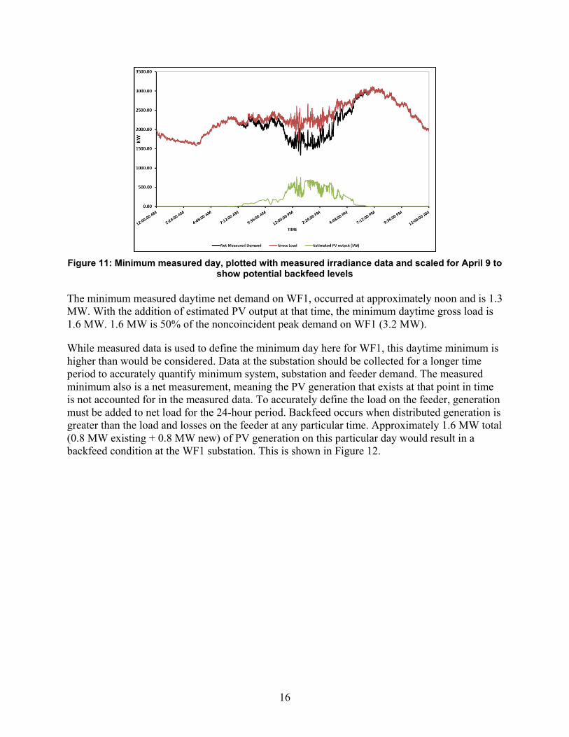
On Saturday April 9th there was approximately 800 kW of PV installed on WF1. The measured substation and feeder demand does not account for this existing generation and is therefore the net demand. The actual gross load is unknown on WF1 at the time of analysis. To accurately quantify the minimum daytime gross load on the feeder, irradiance data for the three local sensors is extracted, plotted with the minimum daytime load, and extrapolated to find the minimum daytime gross demand level on this day (Figure 11).

16

Figure 11: Minimum measured day, plotted with measured irradiance data and scaled for April 9 to

show potential backfeed levels The minimum measured daytime net demand on WF1, occurred at approximately noon and is 1.3 MW. With the addition of estimated PV output at that time, the minimum daytime gross load is 1.6 MW. 1.6 MW is 50% of the noncoincident peak demand on WF1 (3.2 MW).

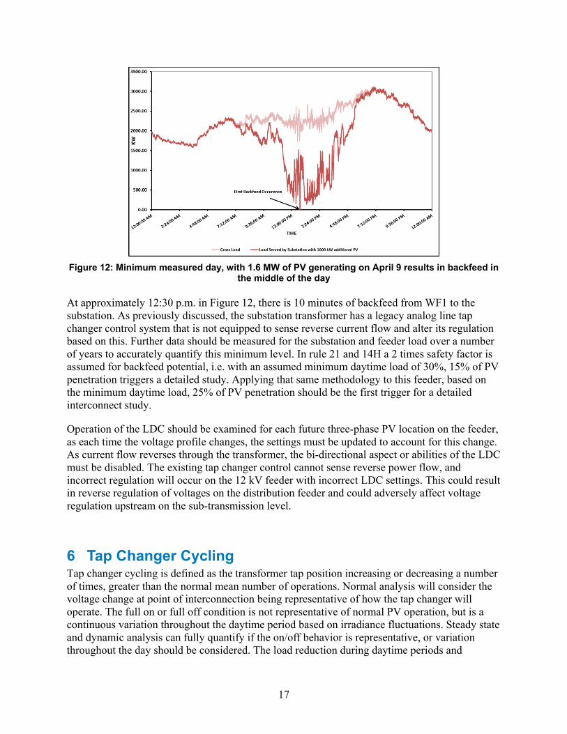
While measured data is used to define the minimum day here for WF1, this daytime minimum is higher than would be considered. Data at the substation should be collected for a longer time period to accurately quantify minimum system, substation and feeder demand. The measured minimum also is a net measurement, meaning the PV generation that exists at that point in time is not accounted for in the measured data. To accurately define the load on the feeder, generation must be added to net load for the 24-hour period. Backfeed occurs when distributed generation is greater than the load and losses on the feeder at any particular time. Approximately 1.6 MW total (0.8 MW existing + 0.8 MW new) of PV generation on this particular day would result in a backfeed condition at the WF1 substation. This is shown in Figure 12.

17

Figure 12: Minimum measured day, with 1.6 MW of PV generating on April 9 results in backfeed in

the middle of the day At approximately 12:30 p.m. in Figure 12, there is 10 minutes of backfeed from WF1 to the substation. As previously discussed, the substation transformer has a legacy analog line tap changer control system that is not equipped to sense reverse current flow and alter its regulation based on this. Further data should be measured for the substation and feeder load over a number of years to accurately quantify this minimum level. In rule 21 and 14H a 2 times safety factor is assumed for backfeed potential, i.e. with an assumed minimum daytime load of 30%, 15% of PV penetration triggers a detailed study. Applying that same methodology to this feeder, based on the minimum daytime load, 25% of PV penetration should be the first trigger for a detailed interconnect study.

Operation of the LDC should be examined for each future three-phase PV location on the feeder, as each time the voltage profile changes, the settings must be updated to account for this change. As current flow reverses through the transformer, the bi-directional aspect or abilities of the LDC must be disabled. The existing tap changer control cannot sense reverse power flow, and incorrect regulation will occur on the 12 kV feeder with incorrect LDC settings. This could result in reverse regulation of voltages on the distribution feeder and could adversely affect voltage regulation upstream on the sub-transmission level.

6 Tap Changer Cycling Tap changer cycling is defined as the transformer tap position increasing or decreasing a number of times, greater than the normal mean number of operations. Normal analysis will consider the voltage change at point of interconnection being representative of how the tap changer will operate. The full on or full off condition is not representative of normal PV operation, but is a continuous variation throughout the daytime period based on irradiance fluctuations. Steady state and dynamic analysis can fully quantify if the on/off behavior is representative, or variation throughout the day should be considered. The load reduction during daytime periods and

18

therefore increased ramp up and down of power supplied by the substation transformer is also considered.

Tap changers alter the voltage at the substation source to the feeder depending on a measured value of voltage. The W1 transformer on average performs 5 operations a day. If the number increases by 1 or 2 operations based solely on PV operation, this analysis considers it a limiting factor for PV installation. Operations and measured evidence have recently shown that this tap changer is now operating more frequently as the PV levels increase. Effects of tap changer cycling can result in life reduction for the transformer, localized heating and wear on the tap changer parts. While the lifetime of the particular tap changer is not analyzed in this study, if a 2 position increase was seen throughout the year this represents a 40% increase in operation times (above mean). Lifetime of mechanical equipment, including tap changers, is defined based on number of operations. A 40% to 50% decrease in time taken to reach this limitation is therefore considered a major impact for WF1. This analysis and comparison to measured data enables a greater understanding of these impacts on a steady state and dynamic level. Switching impacts are decoupled from irradiance fluctuations. Short-term and long-term impacts are validated using the steady state SynerGEE model of WF1. Future impacts can now be determined as PV generation increases and the results extrapolated to quantify lifetime reduction.

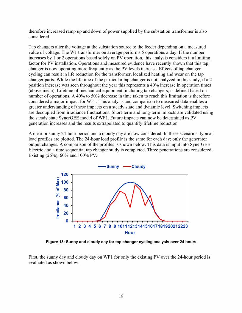
A clear or sunny 24-hour period and a cloudy day are now considered. In these scenarios, typical load profiles are plotted. The 24-hour load profile is the same for each day; only the generator output changes. A comparison of the profiles is shown below. This data is input into SynerGEE Electric and a time sequential tap changer study is completed. Three penetrations are considered, Existing (26%), 60% and 100% PV.

Figure 13: Sunny and cloudy day for tap changer cycling analysis over 24 hours

First, the sunny day and cloudy day on WF1 for only the existing PV over the 24-hour period is evaluated as shown below.

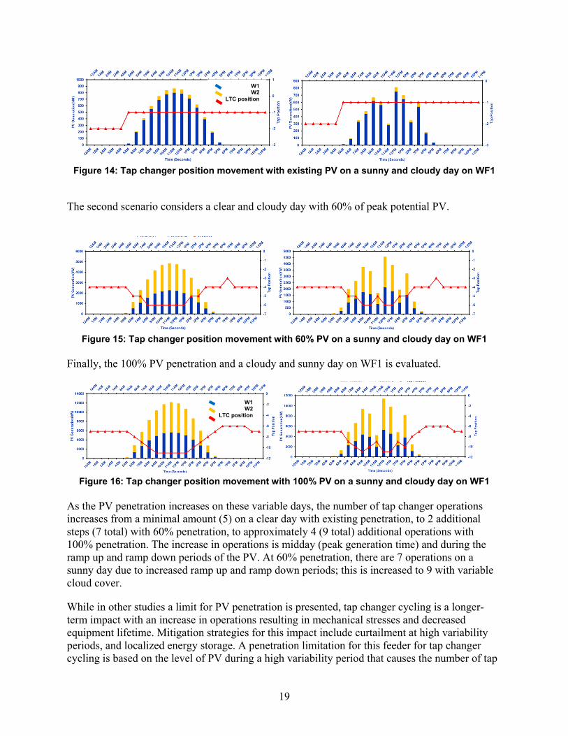
19

Figure 14: Tap changer position movement with existing PV on a sunny and cloudy day on WF1

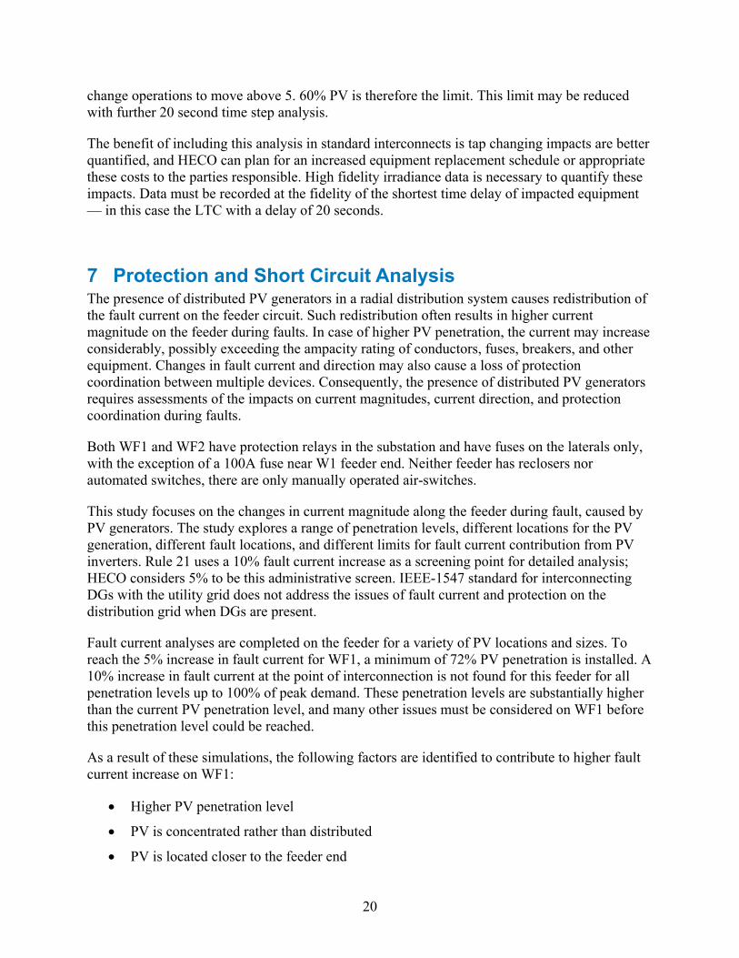
The second scenario considers a clear and cloudy day with 60% of peak potential PV.

Figure 15: Tap changer position movement with 60% PV on a sunny and cloudy day on WF1

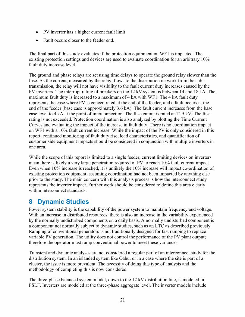
Finally, the 100% PV penetration and a cloudy and sunny day on WF1 is evaluated.

Figure 16: Tap changer position movement with 100% PV on a sunny and cloudy day on WF1

As the PV penetration increases on these variable days, the number of tap changer operations increases from a minimal amount (5) on a clear day with existing penetration, to 2 additional steps (7 total) with 60% penetration, to approximately 4 (9 total) additional operations with 100% penetration. The increase in operations is midday (peak generation time) and during the ramp up and ramp down periods of the PV. At 60% penetration, there are 7 operations on a sunny day due to increased ramp up and ramp down periods; this is increased to 9 with variable cloud cover.

While in other studies a limit for PV penetration is presented, tap changer cycling is a longer-term impact with an increase in operations resulting in mechanical stresses and decreased equipment lifetime. Mitigation strategies for this impact include curtailment at high variability periods, and localized energy storage. A penetration limitation for this feeder for tap changer cycling is based on the level of PV during a high variability period that causes the number of tap

W1 W2

LTC position

W1 W2

LTC position

20

change operations to move above 5. 60% PV is therefore the limit. This limit may be reduced with further 20 second time step analysis.

The benefit of including this analysis in standard interconnects is tap changing impacts are better quantified, and HECO can plan for an increased equipment replacement schedule or appropriate these costs to the parties responsible. High fidelity irradiance data is necessary to quantify these impacts. Data must be recorded at the fidelity of the shortest time delay of impacted equipment — in this case the LTC with a delay of 20 seconds.

7 Protection and Short Circuit Analysis The presence of distributed PV generators in a radial distribution system causes redistribution of the fault current on the feeder circuit. Such redistribution often results in higher current magnitude on the feeder during faults. In case of higher PV penetration, the current may increase considerably, possibly exceeding the ampacity rating of conductors, fuses, breakers, and other equipment. Changes in fault current and direction may also cause a loss of protection coordination between multiple devices. Consequently, the presence of distributed PV generators requires assessments of the impacts on current magnitudes, current direction, and protection coordination during faults.

Both WF1 and WF2 have protection relays in the substation and have fuses on the laterals only, with the exception of a 100A fuse near W1 feeder end. Neither feeder has reclosers nor automated switches, there are only manually operated air-switches.

This study focuses on the changes in current magnitude along the feeder during fault, caused by PV generators. The study explores a range of penetration levels, different locations for the PV generation, different fault locations, and different limits for fault current contribution from PV inverters. Rule 21 uses a 10% fault current increase as a screening point for detailed analysis; HECO considers 5% to be this administrative screen. IEEE-1547 standard for interconnecting DGs with the utility grid does not address the issues of fault current and protection on the distribution grid when DGs are present.

Fault current analyses are completed on the feeder for a variety of PV locations and sizes. To reach the 5% increase in fault current for WF1, a minimum of 72% PV penetration is installed. A 10% increase in fault current at the point of interconnection is not found for this feeder for all penetration levels up to 100% of peak demand. These penetration levels are substantially higher than the current PV penetration level, and many other issues must be considered on WF1 before this penetration level could be reached.

As a result of these simulations, the following factors are identified to contribute to higher fault current increase on WF1:

• Higher PV penetration level

• PV is concentrated rather than distributed

• PV is located closer to the feeder end

21

• PV inverter has a higher current fault limit

• Fault occurs closer to the feeder end.

The final part of this study evaluates if the protection equipment on WF1 is impacted. The existing protection settings and devices are used to evaluate coordination for an arbitrary 10% fault duty increase level.

The ground and phase relays are set using time delays to operate the ground relay slower than the fuse. As the current, measured by the relay, flows to the distribution network from the sub-transmission, the relay will not have visibility to the fault current duty increases caused by the PV inverters. The interrupt rating of breakers on the 12 kV system is between 14 and 18 kA. The maximum fault duty is increased to a maximum of 4 kA with WF1. The 4 kA fault duty represents the case where PV is concentrated at the end of the feeder, and a fault occurs at the end of the feeder (base case is approximately 3.6 kA). The fault current increases from the base case level to 4 kA at the point of interconnection. The fuse cutout is rated at 12.5 kV. The fuse rating is not exceeded. Protection coordination is also analyzed by plotting the Time Current Curves and evaluating the impact of the increase in fault duty. There is no coordination impact on WF1 with a 10% fault current increase. While the impact of the PV is only considered in this report, continued monitoring of fault duty rise, load characteristics, and quantification of customer side equipment impacts should be considered in conjunction with multiple inverters in one area.

While the scope of this report is limited to a single feeder, current limiting devices on inverters mean there is likely a very large penetration required of PV to reach 10% fault current impact. Even when 10% increase is reached, it is unlikely the 10% increase will impact co-ordination of existing protection equipment, assuming coordination had not been impacted by anything else prior to the study. The main concern with this analysis process is how the interconnect study represents the inverter impact. Further work should be considered to define this area clearly within interconnect standards.

8 Dynamic Studies Power system stability is the capability of the power system to maintain frequency and voltage. With an increase in distributed resources, there is also an increase in the variability experienced by the normally undisturbed components on a daily basis. A normally undisturbed component is a component not normally subject to dynamic studies, such as an LTC as described previously. Ramping of conventional generators is not traditionally designed for fast ramping to replace variable PV generation. The utility does not control the performance of the PV plant output; therefore the operator must ramp conventional power to meet these variances.

Transient and dynamic analyses are not considered a regular part of an interconnect study for the distribution system. In an islanded system like Oahu, or in a case where the site is part of a cluster, the issue is more prevalent. The necessity of doing this type of analysis and the methodology of completing this is now considered.

The three-phase balanced system model, down to the 12 kV distribution line, is modeled in PSLF. Inverters are modeled at the three-phase aggregate level. The inverter models include

22

generic response characteristics and under-over frequency protection. Scenarios considered part of the dynamic analysis include:

• N-1 Fault Conditions

• Single Conventional Generator Trip

• Single Transmission (138 kV) Line Trip

• All PV Trip

• Voltage Flicker caused by Irradiance.

These conditions are considered based on the conclusions extracted from measured data on frequency of switching on the feeder (Section 4 showed a large number of switching load changes on WF1). All PV trip can be considered in a steady state analysis, but the dynamic response can contribute more to feeder impacts such as undervoltage, resulting in nuisance protection operation, voltage regulation equipment disturbance and loss of load. A final dynamic condition considered is voltage flicker on the distribution system. Highly variable conditions on a high PV feeder have been perceived as contributing to flicker. The validity of considering a step response versus a time varying irradiance response is considered.

8.1 N-1 Dynamic Analysis N-1 conditions are generally outside the scope of a distribution interconnection study, but since this study seeks to identify if analyses not normally considered are of interest in High PV scenarios, we consider it here. Standard HECO transmission planning contingencies are considered first, i.e. N-1 Scenarios. Extra measurement models are added for the analysis around the area of interest, particularly the following;

• System Frequency

• Voltage at end of feeder

• Voltage at beginning of feeder 12 kV side

• Voltage at beginning of feeder 46 kV side

• Voltage at beginning of feeder 46 kV line.

In the example below, the largest single conventional generator for HECO is tripped at 5 seconds into the simulation. High PV on WF1 (approximately 60% of peak capacity) and High PV penetration in the W1 Area (8 MW on the distribution side, approximately 25% of noncoincident peak for the sum of all feeders in the W1 Area) is considered. The system frequency is plotted first (Figure 17).

23

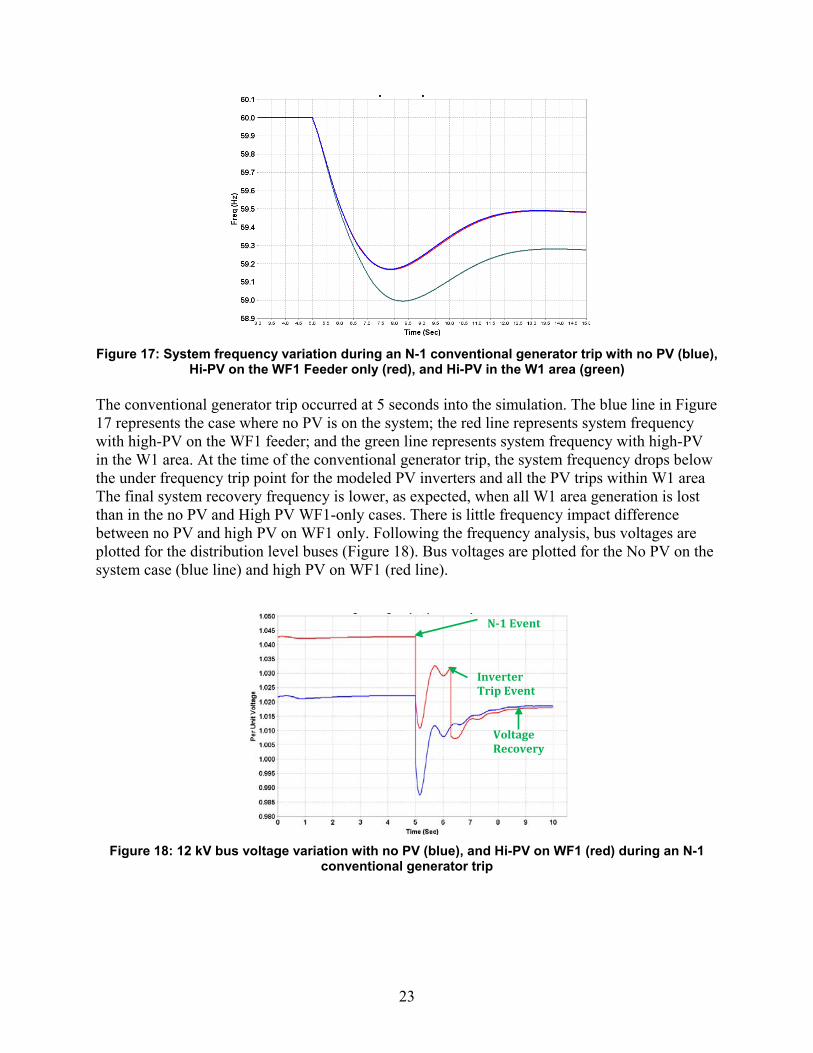
Figure 17: System frequency variation during an N-1 conventional generator trip with no PV (blue),

Hi-PV on the WF1 Feeder only (red), and Hi-PV in the W1 area (green) The conventional generator trip occurred at 5 seconds into the simulation. The blue line in Figure 17 represents the case where no PV is on the system; the red line represents system frequency with high-PV on the WF1 feeder; and the green line represents system frequency with high-PV in the W1 area. At the time of the conventional generator trip, the system frequency drops below the under frequency trip point for the modeled PV inverters and all the PV trips within W1 area The final system recovery frequency is lower, as expected, when all W1 area generation is lost than in the no PV and High PV WF1-only cases. There is little frequency impact difference between no PV and high PV on WF1 only. Following the frequency analysis, bus voltages are plotted for the distribution level buses (Figure 18). Bus voltages are plotted for the No PV on the system case (blue line) and high PV on WF1 (red line).

Figure 18: 12 kV bus voltage variation with no PV (blue), and Hi-PV on WF1 (red) during an N-1

conventional generator trip

N-1 Event

Inverter Trip Event

Voltage Recovery

24

Comparing the no PV penetration and high PV penetration cases, for bus voltage at the 12 kV and 46 kV level; the blue line represents the no PV case voltage measurement, and the red line represents the High PV case. The voltages at the end and beginning of the 12 kV are initially approximately 0.01 per unit different. When the fault occurs the voltage deviation at the end of the feeder, with no PV, is approximately 4% during the transient, then recovers to 1 per unit in approximately 0.7s. In the high PV case, the initial voltage transient is approximately 3.5% and then the voltage starts to recover after a similar time indicated in the no PV case. Approximately 1 second into the fault there is an under-frequency trip of the PV inverters on WF1, and the voltage again drops by approximately 3%. In total the voltage recover takes approximately 0.7 seconds longer then in the no PV case. While the voltage transient is significant, it is not increased due to the secondary PV generator trip. The longer voltage recovery could impact the operation of protection equipment and should be investigated further.

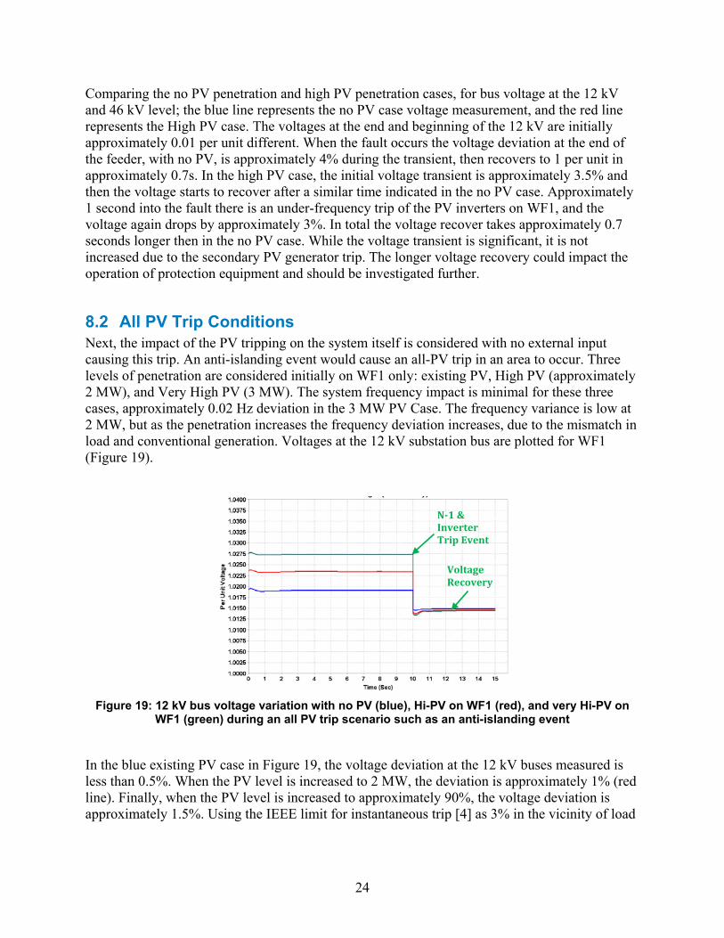
8.2 All PV Trip Conditions Next, the impact of the PV tripping on the system itself is considered with no external input causing this trip. An anti-islanding event would cause an all-PV trip in an area to occur. Three levels of penetration are considered initially on WF1 only: existing PV, High PV (approximately 2 MW), and Very High PV (3 MW). The system frequency impact is minimal for these three cases, approximately 0.02 Hz deviation in the 3 MW PV Case. The frequency variance is low at 2 MW, but as the penetration increases the frequency deviation increases, due to the mismatch in load and conventional generation. Voltages at the 12 kV substation bus are plotted for WF1 (Figure 19).

Figure 19: 12 kV bus voltage variation with no PV (blue), Hi-PV on WF1 (red), and very Hi-PV on

WF1 (green) during an all PV trip scenario such as an anti-islanding event

In the blue existing PV case in Figure 19, the voltage deviation at the 12 kV buses measured is less than 0.5%. When the PV level is increased to 2 MW, the deviation is approximately 1% (red line). Finally, when the PV level is increased to approximately 90%, the voltage deviation is approximately 1.5%. Using the IEEE limit for instantaneous trip [4] as 3% in the vicinity of load

Voltage Recovery

N-1 & Inverter Trip Event

25

served customers, the PV penetrations on feeder WF1 do not exceed dynamic limitations during an All PV trip.

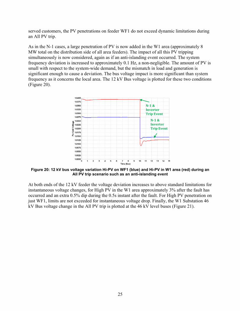
As in the N-1 cases, a large penetration of PV is now added in the W1 area (approximately 8 MW total on the distribution side of all area feeders). The impact of all this PV tripping simultaneously is now considered, again as if an anti-islanding event occurred. The system frequency deviation is increased to approximately 0.1 Hz, a non-negligible. The amount of PV is small with respect to the system-wide demand, but the mismatch in load and generation is significant enough to cause a deviation. The bus voltage impact is more significant than system frequency as it concerns the local area. The 12 kV Bus voltage is plotted for these two conditions (Figure 20).

Figure 20: 12 kV bus voltage variation Hi-PV on WF1 (blue) and Hi-PV in W1 area (red) during an

All PV trip scenario such as an anti-islanding event At both ends of the 12 kV feeder the voltage deviation increases to above standard limitations for instantaneous voltage changes, for High PV in the W1 area approximately 3% after the fault has occurred and an extra 0.5% dip during the 0.5s instant after the fault. For High PV penetration on just WF1, limits are not exceeded for instantaneous voltage drop. Finally, the W1 Substation 46 kV Bus voltage change in the All PV trip is plotted at the 46 kV level buses (Figure 21).

N-1 & Inverter Trip Event

N-1 & Inverter Trip Event

26

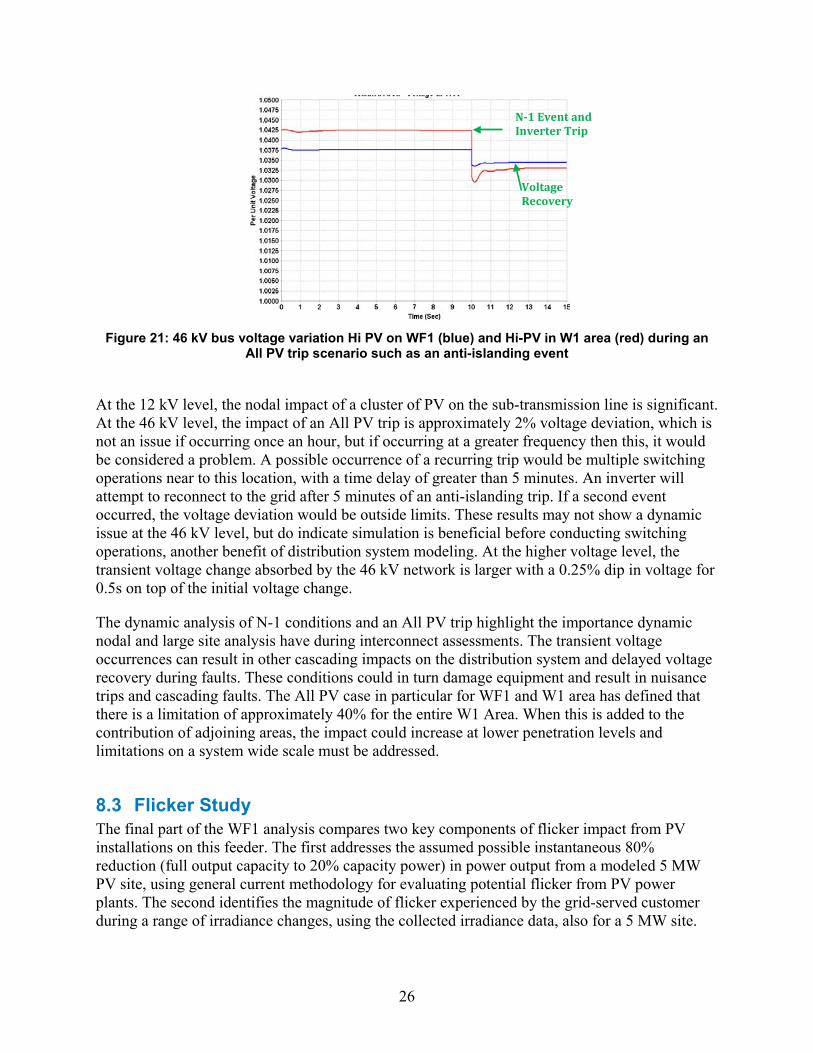
Figure 21: 46 kV bus voltage variation Hi PV on WF1 (blue) and Hi-PV in W1 area (red) during an

All PV trip scenario such as an anti-islanding event

At the 12 kV level, the nodal impact of a cluster of PV on the sub-transmission line is significant. At the 46 kV level, the impact of an All PV trip is approximately 2% voltage deviation, which is not an issue if occurring once an hour, but if occurring at a greater frequency then this, it would be considered a problem. A possible occurrence of a recurring trip would be multiple switching operations near to this location, with a time delay of greater than 5 minutes. An inverter will attempt to reconnect to the grid after 5 minutes of an anti-islanding trip. If a second event occurred, the voltage deviation would be outside limits. These results may not show a dynamic issue at the 46 kV level, but do indicate simulation is beneficial before conducting switching operations, another benefit of distribution system modeling. At the higher voltage level, the transient voltage change absorbed by the 46 kV network is larger with a 0.25% dip in voltage for 0.5s on top of the initial voltage change.

The dynamic analysis of N-1 conditions and an All PV trip highlight the importance dynamic nodal and large site analysis have during interconnect assessments. The transient voltage occurrences can result in other cascading impacts on the distribution system and delayed voltage recovery during faults. These conditions could in turn damage equipment and result in nuisance trips and cascading faults. The All PV case in particular for WF1 and W1 area has defined that there is a limitation of approximately 40% for the entire W1 Area. When this is added to the contribution of adjoining areas, the impact could increase at lower penetration levels and limitations on a system wide scale must be addressed.

8.3 Flicker Study The final part of the WF1 analysis compares two key components of flicker impact from PV installations on this feeder. The first addresses the assumed possible instantaneous 80% reduction (full output capacity to 20% capacity power) in power output from a modeled 5 MW PV site, using general current methodology for evaluating potential flicker from PV power plants. The second identifies the magnitude of flicker experienced by the grid-served customer during a range of irradiance changes, using the collected irradiance data, also for a 5 MW site.

N-1 Event and Inverter Trip

Voltage Recovery

27

The study methodology for flicker used here is the subject of an IEEE PES 2012 General Meeting Paper by the same authors as this report [6].

Flicker is defined as a rapid objectionable change in light level often produced by voltage fluctuations [8]. Standard interconnect processes for utility-scale photovoltaic generators often include a limited voltage flicker study. High-fidelity irradiance data is often not available and thus not considered part of this analysis. A more simplified power output change from rated capacity to an arbitrary 20% or 0% output is considered. Flicker is typically not measured by utilities but based on a customer (with load served by the utility) raising an issue or complaint. IEEE Standard 519 defines power quality implications of distributed generation and the applicable levels at which flicker is a visible or irritable issue. This analysis seeks to inform and improve the flicker simulation methodology, moving away from the standard assumption of instantaneous trip, to an irradiance-based input methodology that is more representative of PV resources.

The occurrence of voltage flicker is generally more prevalent on weak systems and depends on the strength or stiffness of the system. As proven earlier, this feeder is a strong feeder with a lot of extra capacity, which will dictate the size of source and frequency of fluctuation.

Following the creation of an averaged irradiance sensor grid profile and representative 60 second datasets, two modeling approaches will be taken:

1. Five inverter network with power output controlled by irradiance input

2. Step change in power output from 100% to 0%.

The 5-inverter network is created to represent a 5 MW facility, and the maximum transient voltage deviation at the main collector bus on WF1 is calculated over 60 seconds of each dataset from the representative sensors.

Flicker limitations for PV plant interconnects are defined by HECO using the GE Flicker Curve from IEEE 519-1992. An arbitrary site size is selected, therefore a detailed inverter and panel design and specification is not required.

Voltage measurement models are inserted at three points of interest. The measurement points are identified as Measurement Point 1 0.48 kV collection bus, Measurement Point 2 12 kV point of interconnect, with Measurement Point 3 at the 46 kV substation bus. Only 12 kV results are presented in this summary as it is the main load serving point of interest for power quality issues.

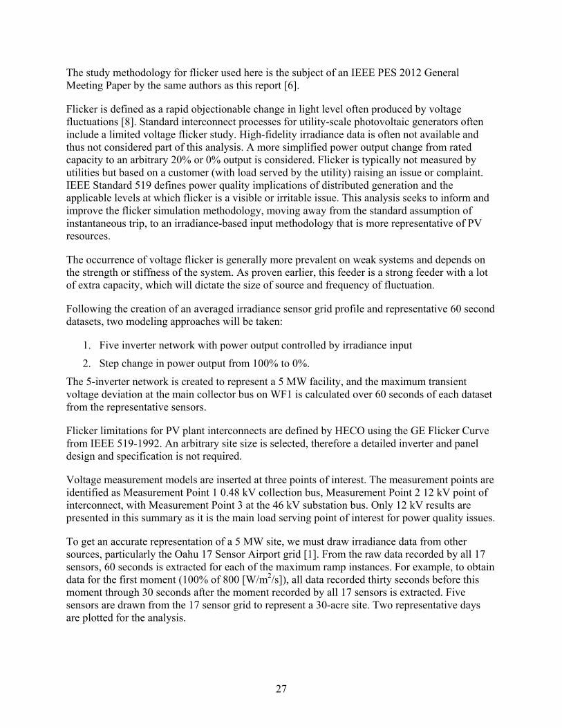
To get an accurate representation of a 5 MW site, we must draw irradiance data from other sources, particularly the Oahu 17 Sensor Airport grid [1]. From the raw data recorded by all 17 sensors, 60 seconds is extracted for each of the maximum ramp instances. For example, to obtain data for the first moment (100% of 800 [W/m2/s]), all data recorded thirty seconds before this moment through 30 seconds after the moment recorded by all 17 sensors is extracted. Five sensors are drawn from the 17 sensor grid to represent a 30-acre site. Two representative days are plotted for the analysis.

28

Figure 22: Irradiance plots of two representative variable irradiance days across 5 sensors from

the Airport irradiance grid for input to the flicker analysis Day 1 is classified as a particularly cloudy day and the outputs of most sensors are at low values of around 20%. Day 2 is a maximum variation on any one sensor of 5% less than the maximum variation day. Day 2 represented a more variable cloud day, with each sensor performing differently.

The most common ramp rate in each month occurs approximately 70% of the time and is less than 100 [W/m2/s]. The 50% level reduction from maximum 400 [W/m2/s] occurs at a minimum of 0 times per month, and a maximum of 0.01% per month (equating to 259 incidences). The maximum ramp rate 800 [W/m2/s] occurred a maximum of 0.0005% in May, equating to 13 incidents of 1 second ramp in one month.

Using the generic inverter model and the irradiance files as proxies for power input to each of the 5 generator models, we ran a 60 second dynamic analysis in PSLF and recorded voltages at each of the key buses. The recorded buses are:

• 0.48 kV Low Side PV Plant Bus

• 12 kV Distribution Point of Interconnection

• 46 kV Sub-Transmission Bus.

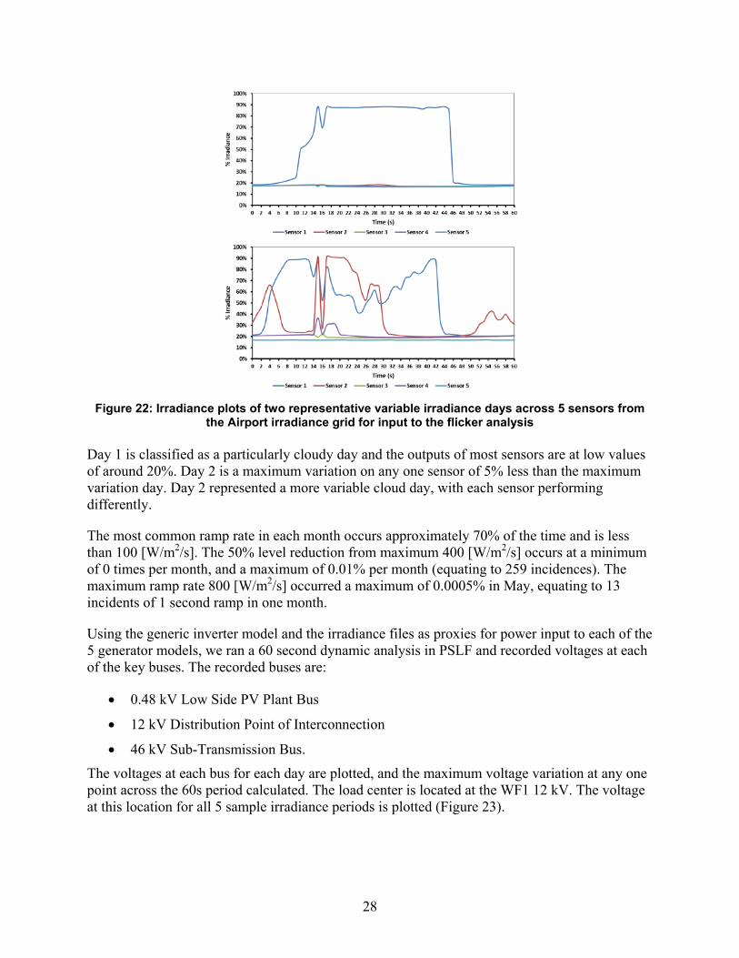
The voltages at each bus for each day are plotted, and the maximum voltage variation at any one point across the 60s period calculated. The load center is located at the WF1 12 kV. The voltage at this location for all 5 sample irradiance periods is plotted (Figure 23).

29

Figure 23: 12 kV bus voltage variation for the 5 highly variable irradiance days input to the

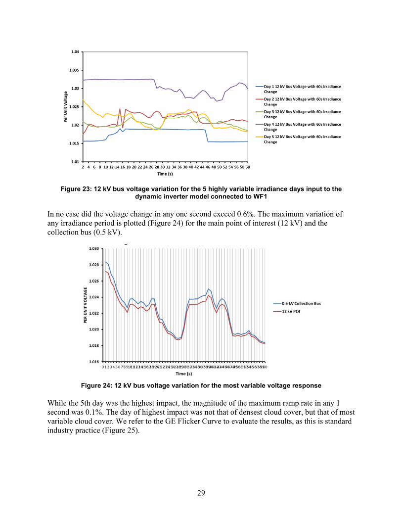
dynamic inverter model connected to WF1 In no case did the voltage change in any one second exceed 0.6%. The maximum variation of any irradiance period is plotted (Figure 24) for the main point of interest (12 kV) and the collection bus (0.5 kV).

Figure 24: 12 kV bus voltage variation for the most variable voltage response While the 5th day was the highest impact, the magnitude of the maximum ramp rate in any 1 second was 0.1%. The day of highest impact was not that of densest cloud cover, but that of most variable cloud cover. We refer to the GE Flicker Curve to evaluate the results, as this is standard industry practice (Figure 25).

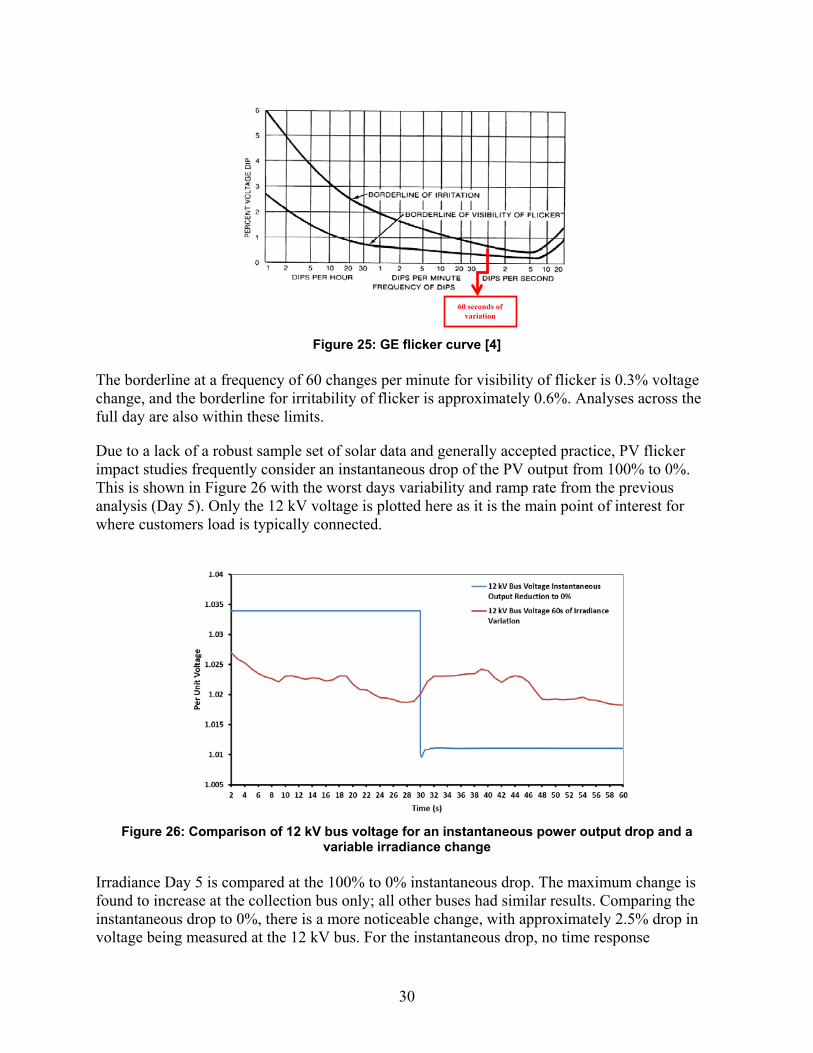
30

Figure 25: GE flicker curve [4] The borderline at a frequency of 60 changes per minute for visibility of flicker is 0.3% voltage change, and the borderline for irritability of flicker is approximately 0.6%. Analyses across the full day are also within these limits.

Due to a lack of a robust sample set of solar data and generally accepted practice, PV flicker impact studies frequently consider an instantaneous drop of the PV output from 100% to 0%. This is shown in Figure 26 with the worst days variability and ramp rate from the previous analysis (Day 5). Only the 12 kV voltage is plotted here as it is the main point of interest for where customers load is typically connected.

Figure 26: Comparison of 12 kV bus voltage for an instantaneous power output drop and a

variable irradiance change Irradiance Day 5 is compared at the 100% to 0% instantaneous drop. The maximum change is found to increase at the collection bus only; all other buses had similar results. Comparing the instantaneous drop to 0%, there is a more noticeable change, with approximately 2.5% drop in voltage being measured at the 12 kV bus. For the instantaneous drop, no time response

60 seconds of variation

31

component is added. If we assume this drop occurred once in an hour, the limitation for visibility of flicker defined by IEEE 519[4] is 3%. If the 5 MW utility scale plant trips offline more than once an hour, among being classified as flicker, this is indicative of other issues and would generally occur during emergencies or N-1 conditions. Therefore, it is not considered a normal operational concern.

9 Conclusions and Future Work 9.1 Limitations Specific to WF1 Steady state impacts are limited to variability results and rare incidents where high voltage should be considered. The lightest load on this conductor is as expected, at the end of the feeder, but on average no conductor is loaded above 19%. The average MVA capacity on this feeder is above 6 MVA (based on average amp rating of all cables and voltage). The peak noncoincident demand is approximately 3.2 MVA. The feeder is therefore sized largely above capacity. It is expected the load flow impacts will be limited due to this overcapacity. Future studies should consider a heavier loaded circuit.

Voltage and thermal limits are normally defined by HECO and other utilities as voltage exceeding 1.05 per unit, and thermal loading exceeding 100%. The voltage and thermal steady state limits are highly dependent on location of PV. No limit is defined for PV penetration on WF1 based on the assumption that no potential PV was added greater than the line thermal limit.

A key finding is the line drop compensation setting, and this directly influenced the finding that backfeed is the main PV penetration limitation on WF1. The tap changer and line drop compensation control equipment type installed at W1 transformer does not sense reverse current flow. It therefore has potential at backfeed levels to cause voltage variations on the subtransmission system. As backfeed could realistically occur during a high generation day in April with only 50% to 55% PV penetration of peak, this issue should be considered the first worst issue to be addressed for WF1. PV generation on WF1 cannot exceed 50% of peak without addressing the backfeed issues. While the lifetime of the particular tap changer is not analyzed in this study, a 2 position change represents a 40% increase in operation times. Lifetime of mechanical equipment, including tap changers, is defined based on number of operations. A 40% to 50% decrease in time taken to reach this limitation is therefore considered a major impact for WF1.

Tap changer cycling can cause a decrease in equipment lifetime. Comparison of measured irradiance, power monitor and validated simulation show that irradiance variations can increase the number of tap changer operations. A limitation for PV penetration is defined in this study, that in simulations of varying irradiance conditions, the number of tap changer operations increasing by 2 is a negative impact, and this occurred with 60% PV penetration on WF1. This impact is more long term than short term, and future analyses should run a year of irradiance and power monitor data to fully establish the yearly increase in operations.

Fault current limitation is defined in this analysis based on point where normal administrative filter is reached (5% for HECO, 10% based on Rule 21 at the point of interconnection). Point of

32

actual impact in this case is not defined. Due to current limiting inverters the 10% filter is not exceeded until above the maximum demand on this feeder.

Dynamic studies included various N-1 conditions and PV system-wide trip. In dynamic, flicker, and harmonic analyses, the benefit of nodal cluster studies is highlighted and the limitations defined based on a combination of substation, feeder, and area penetrations rather than only single feeder. While no real dynamic limitation based on full capacity of PV penetration on WF1 was found, an anti-islanding trip, for example, could have significant impact on WF1 and the W1 area, with instantaneous voltage variations exceeding IEEE limitations at approximately 25% penetration (across all W1 substations, based on noncoincident peak demand). Conventional N-1 conditions such as a generator trip or line trip can cause delayed system voltage recovery. Generator dispatch was fixed in these cases, and modifications are outside the scope of this study.

The final issue considered was flicker, directly linked to the All PV trip case above. A comparison is presented on an instantaneous trip conditions versus a time varying irradiance output. This part of the analysis sought to redefine how flicker impact is quantified for PV, rather than define a limitation on WF1.

9.2 Comparison to Normal Standards and Interconnect Processes The interconnection process can be a laborious and expensive process for both utilities and developers. If not properly considered using realistic data, this may lead to project time delays and potential gaps in the analysis. Ongoing work focuses on improving the interconnection process by identifying real issues with increasing levels of PV at the distribution level versus simply assuming "rules of thumbs" that may no longer benefit the technical conditions emerging today. A number of conclusions are:

• 15% PV penetration triggering a detailed study is low for a single feeder, but significant for a node, cluster, system area (this has been updated in subsequent releases of rule 14H, December 2011)

• Feeder model validation is essential

• Steady state variability and long term equipment impacts should be quantified with measured data

• Minimum daytime load levels must be considered for voltage trends, backfeed potential, and variability/tap changer cycling impacts

• Currently under Rule 14H only peak loads are considered

• California rule 21: do consider minimum daytime load conditions

• Penetration limits/analysis triggers should be defined at minimum daytime demand levels, 12 kV feeder, node and cluster levels based on 46 kV lines.

• Methodology for flicker studies follows guidelines not designed for high penetrations of PV

• Nodal (substation and feeders) and Cluster Studies (collection of nodes) could reduce initial labor for developers and utilities, and spread the cost over the long term.

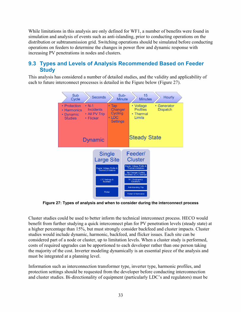
33

While limitations in this analysis are only defined for WF1, a number of benefits were found in simulation and analysis of events such as anti-islanding, prior to conducting operations on the distribution or subtransmission grid. Switching operations should be simulated before conducting operations on feeders to determine the changes in power flow and dynamic response with increasing PV penetrations in nodes and clusters.

9.3 Types and Levels of Analysis Recommended Based on Feeder Study

This analysis has considered a number of detailed studies, and the validity and applicability of each to future interconnect processes is detailed in the Figure below (Figure 27).

Figure 27: Types of analysis and when to consider during the interconnect process

Cluster studies could be used to better inform the technical interconnect process. HECO would benefit from further studying a quick interconnect plan for PV penetration levels (steady state) at a higher percentage than 15%, but must strongly consider backfeed and cluster impacts. Cluster studies would include dynamic, harmonic, backfeed, and flicker issues. Each site can be considered part of a node or cluster, up to limitation levels. When a cluster study is performed, costs of required upgrades can be apportioned to each developer rather than one person taking the majority of the cost. Inverter modeling dynamically is an essential piece of the analysis and must be integrated at a planning level.

Information such as interconnection transformer type, inverter type, harmonic profiles, and protection settings should be requested from the developer before conducting interconnection and cluster studies. Bi-directionality of equipment (particularly LDC’s and regulators) must be

34

investigated. Transformer LTC and LDC settings should be reviewed with each interconnect, especially in legacy equipment.

9.4 Future Work Many different types of software were used in this analysis, and the industry must move towards synchronized software formats in the future. Further work should consider a weaker system or more advanced (composite) load modeling to further define impacts. Future work could expand this analysis to considering the following issues:

• Load refinement and composite modeling

• Detailed generation dispatch analysis

• Nodal variability impacts.

35

10 References

[1] U.S. Department Of Energy HiP-PV Penetration Portal <https://solarhighpen.energy.gov/projects/cpucs_csi_rdd_high_penetration_solar_projects>

[2] National Renewable Energy Laboratory Measurement and Instrumentation Data Centre <http://www.nrel.gov/midc>

[3] IEEE 1547-2003: Standard for Interconnecting Distributed Resources with Electric Power Systems, IEEE, 2003

[4] IEEE Standard 519-1992: Recommended Practices and Requirements for Harmonic Control in Electrical Power Systems, IEEE, 1993

[5] IEEE Standard C57.12.00: General Requirements for Liquid Immersed Distribution Power and Regulating Transformers, IEEE 2010

[6] Electric Power Systems and Equipment—Voltage Ratings (60 Hertz),ANSI Standard Publication no. ANSI C84.1-1995.

[7] E.M. Stewart, T.P. Aukai, et. al "A Realistic Irradiance-based Voltage Flicker Analysis of PV Applied to Hawaii Distribution Feeders" July 2012, IEEE PES General Meeting Transactions (Accepted)

[8] G.C. Cornfield, "Definition and Measurement of Voltage Flicker in Lighting" IEE Colloquium on Electronics in Power Systems Measurement. pp. 4/1 - 4/4, Aug 2002