Embed Size (px)
Citation preview

University of Nebraska - LincolnDigitalCommons@University of Nebraska - Lincoln
Dissertations & Theses in Natural Resources Natural Resources, School of
7-2018
Analysis of Gravity Recovery and ClimateExperiment (GRACE) Satellite-Derived Data as aGroundwater and Drought Monitoring ToolAnthony James MuciaUniversity of Nebraska-Lincoln, [email protected]
Follow this and additional works at: http://digitalcommons.unl.edu/natresdiss
Part of the Hydrology Commons, Natural Resources and Conservation Commons, NaturalResources Management and Policy Commons, Other Environmental Sciences Commons, and theWater Resource Management Commons
This Article is brought to you for free and open access by the Natural Resources, School of at DigitalCommons@University of Nebraska - Lincoln. Ithas been accepted for inclusion in Dissertations & Theses in Natural Resources by an authorized administrator of DigitalCommons@University ofNebraska - Lincoln.
Mucia, Anthony James, "Analysis of Gravity Recovery and Climate Experiment (GRACE) Satellite-Derived Data as a Groundwaterand Drought Monitoring Tool" (2018). Dissertations & Theses in Natural Resources. 265.http://digitalcommons.unl.edu/natresdiss/265

ANALYSIS OF GRAVITY RECOVERY AND CLIMATE EXPERIMENT (GRACE)
SATELLITE-DERIVED DATA AS A GROUNDWATER AND DROUGHT
MONITORING TOOL
by
Anthony James Mucia
A THESIS
Presented to the Faculty of
The Graduate College at the University of Nebraska
In Partial Fulfillment of Requirements
For the Degree of Master of Science
Major: Natural Resource Sciences
Under the Supervision of Professor Tsegaye Tadesse
Lincoln, Nebraska
July, 2018
ANALYSIS OF GRAVITY RECOVERY AND CLIMATE EXPERIMENT (GRACE)
SATELLITE-DERIVED DATA AS A GROUNDWATER AND DROUGHT
MONITORING TOOL
Anthony James Mucia, M.S.
University of Nebraska, 2018
Advisor: Tsegaye Tadesse
This research compares Gravity Recovery and Climate Experiment (GRACE)
groundwater storage (GWS) and root zone soil moisture (RZSM) percentiles to measured
data, other drought indicators (DIs) and indices, and stakeholder observations for the
purpose of assessing the feasibility and usefulness of these products to detect drought
conditions. GRACE percentiles were directly compared to historic groundwater
percentiles at 89 Nebraska well locations. Spatial time-series correlations over CONUS
were performed between GRACE GWS and RZSM and the U.S. Drought Monitor
(USDM), Standardized Precipitation Index (SPI), and soil moisture parameters from
several North American Land Data Assimilation System (NLDAS) models. A survey of
stakeholder observations during a 2016 flash drought event centered on Montana,
Wyoming, South Dakota, and Nebraska was also compared to GRACE percentile data to
analyze drought onset timing, geographic coverage, and severity.
Overall the results show GRACE GWS has similar spatial and temporal
agreement over the well period of record, and generally has the expected negative
correlation relationship with observed groundwater, but it does not accurately reflect
historic percentiles in Nebraska. GRACE GWS and RZSM have moderate correlation

with USDM, and high correlation with SPI, and NLDAS models over the entire U.S. with
notable regional and seasonal patterns. SPI accumulation period also plays an important
role in correlation strength for both RZSM and GWS with the best agreement seen at 3-
month and 12-month accumulation periods, respectively. GRACE RZSM time-series data
closely matches stakeholder observations of decreasing soil moisture availability, while
observations of decreasing water levels were not as closely matched by GWS. When
analyzed as an average over all responding zip codes, RZSM showed an early warning
trend up to six weeks prior to observed reports. These results indicate GRACE
percentiles are promising drought indicators that can be used as a monitoring and early
warning system by decision makers.

iii
ACKNOWLEDGEMENTS
I would like to thank my committee, Dr. Deborah Bathke, Dr. Clint Rowe, Dr.
Tsegaye Tadesse, and Dr. Brian Wardlow, for taking some of their precious time to help
with any questions that I had, attending meetings, and for providing valuable feedback
and recommendations for this research. I would like to especially thank my advisor Dr.
Tsegaye Tadesse for his wonderful support and guidance both with this research and
professionally. I would also like to thank all the people in the School of Natural
Resources who have taken and answered my questions ranging from well databases to
ArcGIS tools. Additionally, the help provided by the UNL Statistics Helpdesk was
pivotal in justifying the use of these correlation comparisons, and the resources provided
by them were fundamental to calculations. The hundreds of participants in the 2016
Northern Plains flash drought survey also deserve recognition as filling out a 16-page
survey is not a quick endeavor, and this research certainly benefited from their input.
Finally, I would like to thank my family and friends for supporting me in pursuing
this degree. All the emails, texts, and phone calls recommending articles on graduate
school and climate research or just their messages of support made this work feel
appreciated and significant. Thank you to my parents, who I have always turned to for
advice and who have instilled the work ethic and determination that made this research
possible.
iv
GRANT INFORMATION
This research was made possible by the following grants for projects which funded the
research time and allowed me to attend graduate school:
1. Providing Drought Information Services for the Nation: the National Drought
Mitigation Center – Department of Commerce – NOAA Grant
NA15OAR4310110.
2. Enhancing Drought Early Warning Capabilities for Agricultural and Tribal
Stakeholders in the Missouri River Basin using Fast Response Drought Indicators
– Department of Commerce - NOAA Climate Program Office (CPO) Sectoral
Applications Research Program (SARP) Grant NA16OAR4310131. Additional
funds to enhance the scope of agricultural producer survey were provided by
NIDIS.

v
Table of Contents
CHAPTER 1 - INTRODUCTION ....................................................................................1
1.1 Motivation ..................................................................................................................1
1.2 Drought Monitoring Background ...............................................................................3
1.3 GRACE Background ..................................................................................................6
CHAPTER 2 - DATA METHODOLOGY ....................................................................10
2.1 Data Processing and Descriptions ............................................................................10
2.1.1 GRACE Percentile Data ....................................................................................10
2.1.2 Groundwater Wells ............................................................................................11
2.1.3 The United States Drought Monitor ..................................................................13
2.1.4 Standardized Precipitation Index .......................................................................15
2.1.5 The North American Land Data Assimilation System Soil Moisture Data ......16
2.1.6 2016 Norther Plains Flash Drought ...................................................................17
2.2 Comparison Methods ...............................................................................................19
2.3 Statistical Methods ...................................................................................................22
CHAPTER 3 - RESULTS ...............................................................................................24
3.1 Groundwater Well Comparison ...............................................................................24
3.2 Spatial Correlations ..................................................................................................27
3.2.1 GRACE - USDM ...............................................................................................28
3.2.2 GRACE - SPI ....................................................................................................35
3.2.3 GRACE - NLDAS .............................................................................................44
3.3 2016 Northern Plains Flash Drought Analysis .........................................................49
3.3.1 Monthly Analysis ..............................................................................................52
3.3.2 Time-Series Analysis.........................................................................................66
CHAPTER 4 - DISCUSSION .........................................................................................70
4.1 Groundwater Well Comparison ...............................................................................70
4.2 Spatial Correlations ..................................................................................................73
4.2.1 GRACE - USDM ...............................................................................................73
4.2.2 GRACE - SPI ....................................................................................................75
4.2.3 GRACE - NLDAS .............................................................................................77
4.3 2016 Northern Plains Flash Drought Analysis .........................................................78

vi
CHAPTER 5 - CONCLUSIONS ....................................................................................81
5.1 Future Work .............................................................................................................82
REFERENCES .................................................................................................................84
APPENDIX I: Flash Drought Stakeholder Survey.......................................................88
APPENDIX II: R Correlation Calculation Code ........................................................104
APPENDIX III: Python Raster Correlation Calculation Code .................................106

vii
List of Multimedia Objects
Table 1: U.S. Drought Monitor drought severity levels and equivalent percentiles to
compare to objective drought indices (Svoboda et al. 2000) .........................................11
Figure 1: Locations of USGS (X) and RTMN (*) wells in Nebraska ............................12
Figure 2: Locations of individual zip codes from which completed surveys were
received ..........................................................................................................................19
Equation 1: Spearman’s Rank Correlation .....................................................................20
Equation 2a: Student T-Test for Correlation Significance .............................................22
Equation 2b: Critical Correlation Values for Significance ............................................22
Table 2: Critical correlations at α < 0.05 for spatial correlations ...................................23
Figure 3: USGS (a) and RTMN (b) correlation values between wells and GRACE
percentiles. The red dot represents the mean, the middle notch represents the median,
and the box represents the 25th and 75th percentiles. ....................................................25
Figure 4: USGS and RTMN well percentiles converted to drought levels correlated
with USDM drought levels. The red dot represents the mean, the middle notch
represents the median, and the box represents the 25th and 75th percentiles ................26
Figure 5: Spatial distribution of GRACE GWS and USGS and RTMN well level
correlation coefficients using the nearest sampling technique. Positive correlations
indicate poor agreement, negative indicate good agreement due to the numbers trending
in opposite directions when showing the same change ..................................................27
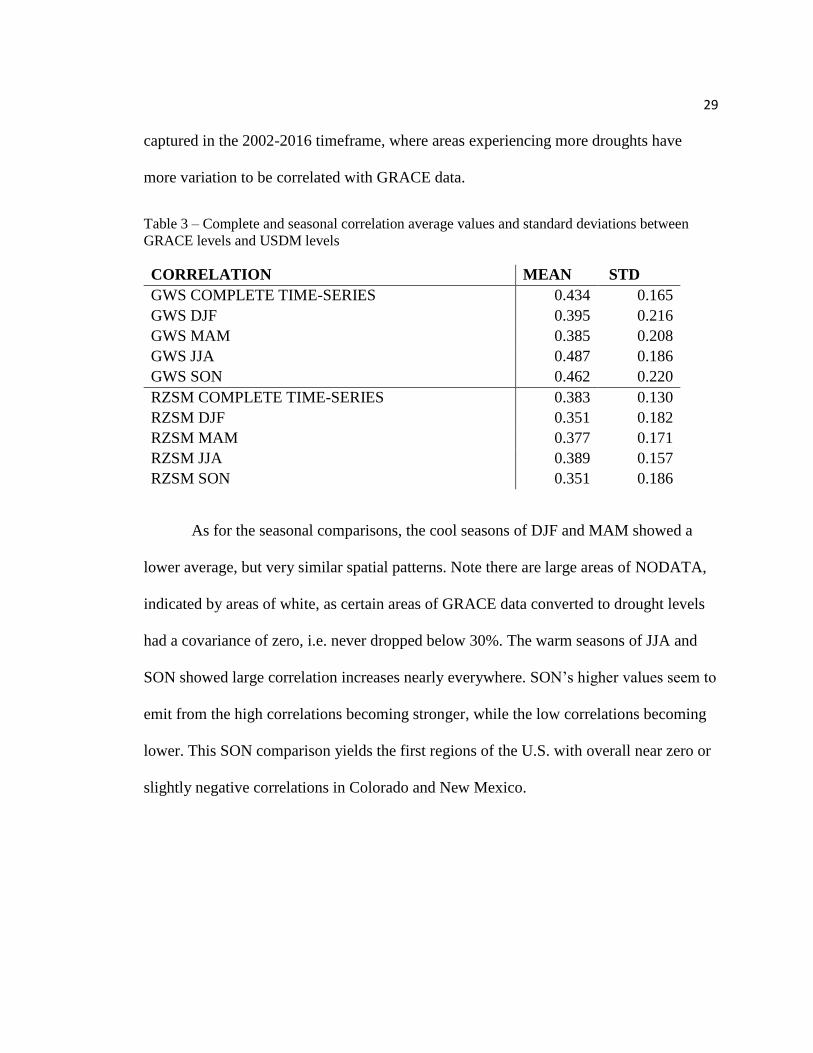
Table 3: Complete and seasonal correlation average values and standard deviations
between GRACE levels and USDM levels ....................................................................29
Figure 6: Correlations between GRACE drought levels and USDM drought levels.
GWS (a), RZSM (b) .......................................................................................................30
Figure 7: Seasonal correlations between GRACE drought levels and USDM drought
levels. GWS (a), RZSM (b) ............................................................................................31
Figure 8: Difference between full period correlations (2002-2016) and truncated period
correlations (2002-2012) for GWS (a) and RZSM (b). Green indicates the full period
correlation are higher, while red indicates the 2002-2012 period correlations are higher
........................................................................................................................................34
Table 4: Correlation average values and standard deviations between GRACE GWS
and RZSM percentiles and SPI anomalies for different accumulation periods .............37
Figure 9: Correlation map values between GRACE GWS and SPI anomalies for
different accumulation periods .......................................................................................38
Figure 10: Correlation map values between GRACE RZSM and SPI anomalies for
different accumulation periods .......................................................................................39
viii
Table 5: Correlation average values and standard deviations between GRACE GWS
and RZSM percentiles and SPI anomalies for different seasons and accumulation
periods ............................................................................................................................41
Figure 11: Correlation values between GRACE GWS percentiles and SPI anomalies
for different seasons and accumulation periods .............................................................42
Figure 12: Correlation values between GRACE RZSM percentiles and SPI anomalies
for different seasons and accumulation periods .............................................................43
Table 6: Correlation average values and standard deviations between GRACE RZSM
percentiles and NLDAS Ensemble (ENS), Noah, and VIC soil moisture percentiles for
different seasons .............................................................................................................45
Figure 13: Correlation values and between GRACE RZSM percentiles and NLDAS
soil moisture percentile ..................................................................................................47
Figure 14: Correlation values and between GRACE RZSM percentiles and NLDAS
soil moisture percentiles for different seasons ...............................................................48
Table 7: Results of stakeholder survey regarding occurrence and start date of drought
conditions .......................................................................................................................50
Figure 15: Maps showing locations where survey respondents observed decreased
topsoil moisture (a), subsoil moisture (b), and lowered water levels (c) with USDM
map valid 31 March 2016 overlaid. Black (blue) hatched areas denote zip codes where
conditions were observed prior to (during) March. Maps showing GRACE RZSM (d)
and GWS (e) valid March 31 where green represents higher percentiles and red low
percentiles .......................................................................................................................53
Figure 16: Same as figure 15 but all images valid 30 April 2016 ..................................55
Figure 17: Same as Figure 15 but all images valid 31 May 2016 ..................................57
Figure 18: Same as Figure 15 but all images valid 30 June 2016 ..................................60
Figure 19: Same as Figure 15 but all images valid 31 July 2016 ...................................63
Figure 20: Same as Figure 15 but all images valid 31 August 2016 ..............................65
Figure 21: Time series average values six weeks prior to six weeks after reports of first
occurrence of decreased topsoil moisture. Left axis is average value of USDM drought
category over each zip code. Right axis is average value of GWS and RZSM
percentiles over each zip code. Left and right axes do not correspond to each other nor
to associated drought level percentiles in Table 1 ..........................................................67
Figure 22: Same as Figure 21, but with reports of first occurrence of decreased subsoil
moisture ..........................................................................................................................68
Figure 23: Same as Figure 21, but with reports of first occurrence of lowered water
levels in streams, ponds, or other water sources ............................................................69

ix
Figure 24: Individual well correlation values and their respective periods of record for
both USGS (red circle) and RTMN (blue triangle) well datasets ..................................71
Figure 25: Spatial distribution of individual well correlation values with irrigation
density overlaid ..............................................................................................................73

1
CHAPTER 1 – INTRODUCTION
1.1 Motivation
Drought monitoring is a complex, but important, task in the study of weather and
climate and in reducing societal vulnerability to drought. Economic damages from
droughts have risen in the past decades and drought impact is estimated in billions of
dollars every year in the United States (Smith & Katz 2013, Wilhite, 2000). Depleted
groundwater and soil moisture are some of drought’s most severe effects, causing water
shortages and reduced crop yield (Denmead et al. 1962). Remote sensing and modeling
of drought’s impacts can help quantify through objective measures the extent and severity
of drought, identify the timing of drought onset and conclusion, and determine the
frequency of drought over individual regions.
The National Aeronautics and Space Administration’s (NASA) Gravity Recovery
and Climate Experiment (GRACE) mission has produced groundwater storage and root
zone soil moisture drought indicators (DI) based on satellite gravitational measurements
assimilated into land surface models. These products are calculated as a percentile of the
historic mean (see section 1.3) and thus are directly comparable with other percentile-
based DIs. The monitoring of the severity and timing of droughts through tools like
GRACE DIs helps in providing decision makers with improved, more timely information
to mitigate and respond to this natural disaster.
This research assesses these GRACE percentile DI products by comparing them
against measured data, other known DIs and indices, and the observations of drought by
stakeholders during a notable, recent drought event. This type of assessment is necessary

2
for several reasons. First to determine the accuracy of the GRACE DIs to represent
historic groundwater or soil moisture conditions through the percentile method. The
second is to evaluate the usefulness of GRACE percentile products as DIs. Although
precise estimates of groundwater and soil moisture may have inaccuracies, they still have
value in the relative differences depicted between current and historical conditions. This
is because the drying and wetting trends, that may not accurately reflect historic
percentiles, are still apparent in GRACE DIs for drought events. For example, an event
that GRACE characterizes as dropping from 80% soil moisture to 31% soil moisture
(edge of D0 drought as designated by USDM) may not mean current soil moisture is
ranked historically in the bottom 31% of years, but the rapid drying clearly indicates a
significant effect. The comparison to other DIs can show GRACE’s spatial and seasonal
strengths and weaknesses because of the relatively known strengths and weaknesses of
the more extensively studied DIs.
Currently, spatially continuous, long-term soil moisture datasets in the U.S. are
modeled. These models help in assessing dryness, however the associated uncertainties in
accuracy may lead to choosing other DIs to use to determine drought extent. Sparse
groundwater observations and the resulting spatial interpolations are the only way to
quantify groundwater levels, which are very important to agricultural producers
especially in times of long-term drought. GRACE percentile datasets may help close this
gap in soil moisture and groundwater data. An increase in soil moisture estimate accuracy
and a spatially continuous groundwater dataset would be an invaluable resource for
stakeholders and drought specialists alike.

3
1.2 Drought Monitoring Background
Several decades of research have yielded different definitions for drought (Wilhite
2000). Although they are all connected, different types of droughts can vary by length
and affect local resources differently. In general, meteorological drought is defined as
abnormal periods with low or no precipitation. Hydrological drought deals with the
effects of precipitation working through reservoirs, streamflow, and groundwater.
Agricultural drought is how crops respond to increased heat stress and lack of water
availability in the soil. Finally, socioeconomic drought is associated with economic
supply and demand of goods, such as water and agricultural products, which are heavily
affected by meteorological, hydrological, and agricultural droughts (Wilhite and Glantz
1985). All of these drought types have water in common, and thus monitoring water is a
pivotal aspect to study for all of these sectors (Tallaksen 2004).
Drought monitoring using objective and subjective assessments of weather,
hydrology, agriculture, and human responses is an important part in the goal of
successfully mitigating and responding to drought effects. The widespread use of remote
sensing systems, in acquiring meteorological, hydrological, and vegetation health data,
allows for multiple high spatial resolution, multi-faceted resources to quantify and
respond to drought.
The first quantitative drought indices appeared early in the 20th century as
Munger’s Index and Kincer’s Index (Heim 2002). These indices measured the period of
time without a specific amount of precipitation. Because precipitation is a highly variable
quantity, any fixed amount of precipitation would not be sufficient for all regions. The

4
mid-20th century saw more drought indices evolve to include more than just precipitation,
and specifically analyzed variables necessary for agricultural and hydrological impacts
(Heim 2002). In 1965, Palmer developed the Palmer Drought Severity Index (PDSI) that
accounts for temperature and precipitation in a water balance model (Palmer 1965). This
index was effective at identifying long-term droughts, and accounted for several variables
previously ignored, however it lacked a high degree of comparability between regions
and did not account for snow or ice. The next largest innovation in drought monitoring
was in 1993, with the creation of the Standardized Precipitation Index (SPI), which
determines precipitation surpluses or deficits in terms of anomalies from normal,
allowing uniform calculation in different regions (McKee et al. 1993). While SPI deals
very well with meteorological drought, it has limitations in identifying hydrological and
agricultural droughts (World Meteorological Organization 2012). Additionally, climate-
based drought indices are based on weather station data (sometimes interpolated to a
uniform grid) which are far less dense in remote areas. In contrast, satellite-based indices
have continuous, equal coverage of the entire area of interest.
Modelling and remote sensing have recently become driving forces in drought
monitoring with their ability to look at the large-scale effects of drought. The Normalized
Difference Vegetation Index (NDVI) was one of the first to make use of remotely sensed
imagery as a drought tool (Rouse et al. 1974). Using the normalized differences in
spectral reflectance, vegetation health, often linked to water availability, is assessed.
Hybrid drought indices such as the Vegetation Drought Response Index (VegDRI)
(Brown et al. 2008) use the combined power of remote sensing and observed data to

5
assess drought impacts on vegetation. NLDAS soil moisture (Xia et al. 2012a, Xia et al.
2012b), often used to identify drought events, similarly uses observed data to model soil
moisture at high resolution.
Groundwater, an important resource for agriculture and urban centers, is currently
monitored based on individual well measurements across the country, and usually done at
the natural resource district, state, or aquifer scale. The varying groundwater depths,
terrain, aquifer type, and observation density all contribute to a sparse set of groundwater
data for the United States. Some modeled data based on these observations are also
available, but many are focused at the regional level.
Because of the impacts of drought on state and federal resources, the National
Oceanic and Atmospheric Administration (NOAA), the U.S. Department of Agriculture
(USDA), and the National Drought Mitigation Center (NDMC) have created a weekly
drought monitor map based on several climate and satellite-based DIs and indices, other
in situ measurements and drought expert input from across the United States (Svoboda et
al. 2000). Because drought has no formal, or quantitative definition, U.S. Drought
Monitor (USDM) authors rely on a combination of objective drought indices as well as
subjective expert analysis and regional and local impact reports to create comprehensive
weekly maps of hydrological and agricultural drought conditions for the conterminous
U.S., Alaska, Hawaii, and Puerto Rico.

6
1.3 GRACE Background
Earth’s gravitational changes are measured by the GRACE two-satellite system in
an orbit at an 89.5° inclination, ~500km altitude, in which the satellites are ~220km apart.
A microwave-ranging instrument aboard the satellites measures changes in distance
between the two satellites from which it can create maps of Earth’s changing gravity
field. The primary cause of these changes in gravity are the fluctuations of water mass on
Earth (Tapley et al. 2004). The GRACE satellite system has provided measurements of
gravity changes for the entire globe from April 2002. In October 2017, one of the
satellites suffered a battery failure, causing the mission to conclude (NASA, 2017).
GRACE-Follow On (GRACE FO) was launched in May 2018 and promises to provide
the same hydrologic products as the original mission, while testing several measurement
methods for higher accuracy and precision.
The satellite data are processed at three centers that include the University of
Texas Center for Space Research (CSR), the GeoFroschungsZentrum Potsdam (GFZ),
and NASA’s Jet Propulsion Laboratory (JPL). Each center has a unique processing
algorithm, but with the same main calculations and characteristics. GRACE observed
estimates of total water storage (TWS) are produced at monthly intervals at a spatially
limited 150,000 km2 horizontal resolution (Rowlands et al. 2005, Yeh et al. 2006). The
processed GRACE TWS is a single value comprised of soil moisture, vegetation, surface
water, ice, snow, and groundwater. It represents the entire vertical column at and below
the surface of the Earth. Through several studies, it has been shown that GRACE data can
be effectively integrated into land surface models (LSM) in order to disaggregate

7
components of total water storage changes (TWSC) (Wahr et al. 1998). This
disaggregation is done by subtracting modeled soil moisture and snow water equivalent
from GRACE TWS. Most estimates assume vegetation and surface water to be terms
small enough to negate. GRACE data have been successfully assimilated into LSMs and
disaggregated into terms of snow water equivalent (SWE) (Niu et al, 2007) that improved
estimates of hydrologic state and fluxes (Su et al. 2010 and Forman et al. 2012), root
zone soil moisture (RZMC) (Wahr et al. 1998), and groundwater storage (GWS) (Rodell
et al. 2007).
The GRACE TWS product has been assimilated into the Catchment Land Surface
Model (CLSM) (Koster et al. 2000, Ducharne et al. 2000) and the disaggregated data is
used in this research. This method increases spatial and temporal resolutions and
disaggregates TWS into some of its component parts (groundwater, soil moisture, and
snow water equivalent). The CLSM is configured with a grid centered over the
conterminous United States similar to the North American Land Data Assimilation
System (NLDAS) (Mitchell et al. 2004), and simulated with NLDAS-2 meteorological
and energy flux forcing data (Xia et al. 2012a, Xia et al. 2012b)
The GRACE assimilated CLSM takes forcing data inputs (precipitation, solar
radiation, temperature, wind, humidity, and pressure) and integrates GRACE TWS into
the model using an Ensemble Kalman smoother (Zaitchik et al. 2008, Kumar et al. 2016).
Groundwater and soil moisture have been modeled by CLSM during the 1948-2016
period using historical observations as inputs. The GRACE data assimilated (DA) model

8
products are then calculated as a percentile of the historic conditions and will be assessed
for their usefulness as drought indicators.
GRACE TWS that was disaggregated into groundwater and assimilated into
model simulations was previously evaluated against non-assimilated, open loop model
simulations on a basin scale across the United States (Zaitchik et al. 2008, Houborg et al.
2012). Zaitchik et al. found small, but significant (α < .05) increases in correlations for
three out of five basins (Mississippi, Ohio-Tennessee, and Missouri), with another basin
(Red-Arkansas/Lower Mississippi) seeing significant improvement at α < 0.10 when
compared to the non-assimilated simulation. Houborg et al. found significant (α < .05)
improvement for three basins (Great Basin and Colorado, Upper East Coast, and
Arkansas-Red/Lower Mississippi), while two basins (Missouri and California) saw
statistically significant (α < .05) skill decreases.
This research assesses the relationship between measured groundwater levels and
GRACE groundwater percentiles and compares GRACE percentiles to other DIs and
indices. A GRACE-based DI percentile approach was first examined by Houborg et al. in
2012 in order to translate GRACE-assimilated products such as surface soil moisture,
root zone soil moisture, and groundwater storage into drought indicators consistent with
the U.S. Drought Monitor. While inaccuracies, measurement and computational errors,
and modelling deficiencies can produce notable differences between the absolute
GRACE soil moisture and groundwater estimates and observed data, a percentile
approach for the datasets provides historical context and allows relative comparisons
between the records to assess the general anomalies that are represented. While percentile

9
datasets are sensitive to the total dataset time period and comparing percentile datasets
with different spin-up periods can result in disagreement, the general benefit of spatially
independent historic context is critical when mitigating and making decisions in drought
events. This study analyzes the comparison between GRACE groundwater percentiles
and long-term United States Geological Survey (USGS) groundwater records as well as
between GRACE groundwater percentiles and shorter-term well records from the
Nebraska Real-time Monitoring Network (RTMN). The relationships between GRACE
percentiles and the U.S. Drought Monitor (USDM) (Svoboda et al. 2002), Standardized
Precipitation Index (SPI), and the North American Land Data Assimilation System
(NLDAS) modeled soil moisture are also studied.
10
CHAPTER 2 – DATA AND METHODOLOGY
2.1 Data Processing and Descriptions
As the GRACE satellites launched in March 2002, actively retrieving data since
April 2002, all comparisons are made with the same start date of the first week of April
2002. However, due to the data not being available when this research was conducted,
SPI and NLDAS data comparisons only extend to the end of 2012, whereas groundwater
well and USDM comparisons were extended to the end of 2016.
2.1.1 GRACE Percentile Data
This study uses two GRACE percentile products, groundwater storage (GWS) and
root zone soil moisture (RZSM). These data are produced weekly at 0.125° spatial
resolution (approximately 13.8 x 13.8 km) and the time period of April 2002 – December
2016 is used. These data are in a raster format over the continental United States. Each
cell in the raster contains a single percentage value, ‘0’ representing the driest historical
condition for that location, and ‘100’ representing the wettest condition. Each of the cells
in these data-assimilated percentiles from 2002-2016, calculated from on the historical
model data, on average range from 0.8 – 99.8% for RZSM and 3.2 – 97.3% for GWS.
This large range indicates that both GWS and RZSM products capture nearly all
variability of the historic dataset, and adequately represent trends during this time period.
The original data are processed by clipping the spatial extent to match the exact
boundaries of the continental U.S. (the raw data extended well into Canada and Mexico)
as to match the coverage of the other datasets.

11
Then, these data are copied and separately processed according to the temporal
and spatial resolution of the data to which it was being compared. A set of raster data is
resampled to match the larger spatial resolution of SPI (25 x 25 km) and NLDAS (20.2 x
20.2 km) rasters using the nearest pixel resampling method. The SPI matching dataset
had weekly values which are averaged to monthly values using ArcGIS python scripting.
Finally, for the USDM comparison, GRACE percentiles were reclassified into their
respective drought levels as given by Table 1.
Table 1 – U.S. Drought Monitor drought severity levels and equivalent percentiles to compare to
objective drought indices (Svoboda et al. 2000)
DROUGHT LEVEL PERCENTILE
No Drought 31 - 100
D0 – Abnormally Dry 21 - 30
D1 – Moderate Drought 11 – 20
D2 – Severe Drought 6 -10
D3 – Extreme Drought 3 - 5
D4 – Exceptional Drought 0 -2
2.1.2 Groundwater Wells
To assess GRACE GWS accuracy, values were compared to measured
groundwater well levels across the state of Nebraska. While each well represents only a
single point compared to the GRACE cells of about 190.44 km2 in area, assessing the two
percentile levels and trends can begin to show what level of accuracy the GRACE DI has.

12
Two well datasets are used in this research, the United States Geological Survey (USGS)
daily groundwater data and the Nebraska Real-Time Monitoring Network (RTMN) daily
groundwater data.
The USGS keeps a collection of continuously reporting groundwater wells across
the country (USGS 2016). In Nebraska, USGS maintains 33 of these wells (Figure 1)
with relatively long-term, daily historical records. These well sites measure water levels
as distance from the surface station at least once per day and automatically store and
report the level. This provisional data is put through USGS quality assurance to ensure
consistent and accountable measurements. These wells were selected because their
historical records dating back to at least 1999, maintaining a historical record longer than
the GRACE record. While aquifer type certainly does impact the well level responses to
drought, selection was not based on this characteristic because of the already small
sample size with the stipulation of record length.
Figure 1 - Locations of USGS (X) and RTMN (*) wells in Nebraska

13
The University of Nebraska – Lincoln Institute of Agriculture and Natural
Resources (IANR) has developed a project that provides real-time groundwater level
monitoring across the state of Nebraska (UNL IANR 2017). The RTMN project uses
remote telemetry, smart sensors, and wireless communication to collect and analyze
hydraulic information from 56 locations around Nebraska (Figure 1). These groundwater
levels have generally recent and wide ranging first readings from as early as 2002 to as
late as 2015, but on average they start around 2007. This dataset also has significant gaps
in daily readings, which further limits the value of the data. Despite these limitations, the
data was used in order to gain wide ranging spatial distribution of observed groundwater
levels across Nebraska. The daily well data from both datasets were averaged to weekly
values to match the weekly GRACE data. Weeks with no data (usually caused by
maintenance on the well infrastructure) were omitted from the final datasets.
2.1.3 The United States Drought Monitor
The U.S. Drought Monitor (USDM) was created in 1999 by the U.S. Department
of Agriculture (USDA), the National Oceanic and Atmospheric Administration (NOAA)
and the National Drought Mitigation Center (NDMC) (Svoboda et al. 2002) as a way to
centralize and improve drought monitoring in the United States. The end product is a
weekly map of drought severity (categorized as D0-D4) that incorporates objective
weather and hydrologic data with local, state, regional, and federal input. The categories
(Table 1) correspond to percentiles based on historical data and estimate the frequency of
different drought severities at a given location and time of year.

14
USDM authors selectively incorporate many objective measurements and
observational data such as weather variables (precipitation, temperature, and dewpoint),
hydrologic levels (streamflow, snowpack, and reservoir levels), and vegetation indices
(NDVI and other satellite-based greenness products). However, groundwater and soil
moisture are not heavily represented, mostly due to a lack of observations and limited
data access. GRACE percentile products have been accessible for Drought Monitor
authors for several years (likely since 2013), and each author may have chosen to
incorporate drought as shown by GRACE GWS or RZSM into the Drought Monitor.
However, the accuracy and usefulness of these products had not been fully explored.
Model-based approaches to these hydrologic variables, such as the GRACE groundwater
and soil moisture percentiles evaluated in this research, may assist the Drought Monitor
authors in creating a consistent and accurate representation of drought in the United
States with known biases and patterns. Weekly USDM data were acquired in vector
format (NDMC, USDA, NOAA, 2017) and converted to rasters corresponding to
GRACE’s spatial resolution.
In addition to looking at how GRACE GWS and measured well levels compare,
these well levels were compared to the USDM. This analysis translated the previously
calculated well level percentiles into drought categories (Table 1). This was done to
determine if these specific well levels show any significant relationship with the gold
standard of drought monitoring. While USDM maps do have boundaries indicating
“Short-term” (S) and “Long-term” (L) drought impacts, these impact and drought types
were not considered in the comparisons. While the timeframe of the drought certainly
15
effects impacts, including groundwater and soil moisture analyzed in this research, the
processing to separate impacts in the quantitative comparisons limited this analysis.
Additionally, the spatial designation of the time-scales of drought levels is not entirely
consistent throughout USDM history, with some areas having clearly defined boundaries,
and some areas just with the “S” or “L” placed without any boundaries.
2.1.4 Standardized Precipitation Index
The Standardized Precipitation Index (SPI) is the cumulative probability of a
specific rainfall event occurring (McKee et al. 1993). Historical rainfall data is fitted to a
gamma function to obtain a normal distribution. Time scales are determined by
accumulation periods in months, with shorter time scales showing SPI frequently moving
above and below zero and longer time scales showing fewer fluctuations. Monthly
gridded SPI of 14 different accumulation periods (1 month – 12-month, 18-month, 24-
month) were collected through the NDMC Drought Atlas (HPRCC and NDMC 2017) at
25 x 25 km spatial resolution. This data was previously processed by interpolating station
SPI into the gridded format. While SPI is a measure of only one drought variable,
precipitation, the seasonal meteorological patterns have a large effect on groundwater but
are often only seen much later in time or on larger accumulation ranges. Fiorillo et al
(2010) found SPI is best correlated with river discharge at 9- to 12-month accumulation
periods. Accumulation periods of 12-month or longer also are highly tied to reservoir and
groundwater levels (World Meteorological Organization, 2012). Soil moisture, on the
other hand, would respond quicker to precipitation events. Accumulation periods between

16
1-month and 6-months are associated with soil moisture conditions (World
Meteorological Organization, 2012).
2.1.5 The North American Land Data Assimilation System (NLDAS) Soil Moisture
Data
The North American Land Data Assimilation System (NLDAS) is a quality
controlled, spatially and temporally consistent land surface model (LSM). The project is a
collaboration among NOAA/National Centers for Environmental Prediction’s (NCEP)
Environmental Modeling Center (EMC), NASA’s Goddard Space Flight Center (GSFC),
Princeton University, the University of Washington, NOAA/National Weather Service
(NWS) Office of Hydrological Development (OHD), and NOAA/NCEP Climate
Prediction Center (CPC). Modeled soil moisture percentiles were obtained using two
NLDAS land surface models, Noah (Chen et al. 1996), and Variable Infiltration Capacity
(VIC) (Liang et al. 1994) as well as the ensemble mean of Noah, VIC, Sacramento (SAC)
(Burnash et al. 1973) and Mosaic (Koster and Suarez 1992). Each LSM simulates the
processes of evapotranspiration, drainage, and vegetation uptake and depth slightly
differently, and the output of each model can differ from each other. These LSMs are
used in this research to compare to GRACE soil moisture percentiles as each LSM also
produces soil moisture percentiles as outputs. GWS was not compared as groundwater is
a fundamentally different quantity and NLDAS groundwater was not available for all
models. NLDAS soil moisture data was gathered from NDMC projects at ~20 x 20 km
resolution and produced at weekly intervals. This evaluation uses NLDAS data from
April 2002 to December 2012.

17
2.1.6 2016 Northern Plains Flash Drought
In spring and summer 2016, a flash drought event developed rapidly over the
Northern Plains, centered on western South Dakota, eastern Wyoming, southeastern
Montana and northwestern Nebraska (USDM 2016). Flash drought refers to rapid onset
drought events characterized by extreme atmospheric anomalies that persist for several
weeks. Quickly deteriorating vegetation health, warm surface temperatures, increased
evapotranspiration, and depleted soil moisture are typical conditions seen in flash drought
events (Otkin et al. 2013). This region experienced impacts including forest and grassland
fires, low forage production, decreased water quantity, and plant stress/death contributing
to large economic losses for stakeholders. Through a National Integrated Drought
Information Systems (NIDIS) funded project to study agricultural impacts of flash
droughts and the drought monitoring capabilities of the Evaporative Stress Index (ESI)
and USDM, a survey was sent to agricultural producers in the drought affected region
(IRB#20160816292 EX). This survey was developed with expert input and pretested by
agricultural extension personnel. It included questions focused on the timing and severity
of individual impacts that allows researchers to track the onset and spread of drought.
The survey (Appendix I) was sent to 2389 agricultural producers living in 42
South Dakota, 16 Wyoming, 13 Nebraska, and 13 Montana counties that had experienced
at least abnormally dry (D0) conditions by July 2016 according to USDM. A stratified
random sample was taken that oversampled counties experiencing the most severe
drought levels and undersampled the large number of counties that only experienced
abnormal dryness. This sample was done in order to ensure that a sufficient number of

18
responses were returned from areas experiencing each level of drought severity. The
sampling frame was a list of producers participating in federal farms programs and was
obtained from a Freedom of Information Request to the USDA Farm Services Agency.
The National Drought Mitigation Center (NDMC) administered the survey, with
surveys mailed to the producers using the U.S. Postal Service. Following Dillman et al.
(2009), a pre-survey letter was mailed to each producer in early November 2016,
followed by the initial survey mailing in late November 2016 with a follow up survey
mailing in January 2017. Out of the 2389 surveys mailed out, 516 (22%) were completed
and returned to NDMC, 348 (15%) being completed by agricultural producers. Any
survey not filled out by landowners actively engaged in agricultural production were
excluded from the analysis.
In order to visualize a better spatial resolution of responses, the respondent’s zip
code was used to represent the location of each report. Counties represented too large an
area to assume homogeneity of impacts, while pinpointed locations were not displayed
because many addresses consisted of PO boxes and to respect the respondent’s
information privacy. It should be noted that individual responses could potentially
integrate information from surrounding areas if land was owned in more than one zip
code. Agricultural producer responses from 136 zip codes are represented in Figure 2.

19
Date reports were averaged by zip code to denote the first occurrence of impacts.
Figure 2 – Locations of individual zip codes from which completed surveys were received.
2.2 Comparison Methods
This research employs three main methods of comparing data. The first compared
the gridded GRACE data to measured well point data. For April 2002 to December
2016, well levels were calculated as a percentile rank of the total historic record for that
well. Each well location was sampled from the GRACE GWS time series using two
spatial sampling techniques, nearest and cubic, and compared to well levels and well
percentiles. Nearest sampling takes only the value of the pixel that each location is in,

20
whereas cubic calculates a weighted average value based on the 16 nearest pixels (ESRI
2017).
The two time-series were then compared using Spearman’s Rank Correlation
𝑟𝑠 = 𝜌𝑟𝑔𝑋 , 𝜌𝑟𝑔𝑌 = 𝑐𝑜𝑣(𝑟𝑔𝑋,𝑟𝑔𝑌)
𝜎𝑟𝑔𝑋,𝜎𝑟𝑔𝑌 Eq. 1
where 𝜌 denotes the correlation coefficient for ranked variables, 𝑐𝑜𝑣(𝑟𝑔𝑋 , 𝑟𝑔𝑌) is the
covariance of the ranked variables, and 𝜎𝑟𝑔𝑋 and 𝜎𝑟𝑔𝑌 are the standard deviations of the
ranked variables. Spearman rank correlation was selected as it describes the association
strength between any of the two datasets (GRACE-wells, GRACE-USDM, GRACE-SPI,
and GRACE-NLDAS), while its calculation assumptions also fit the data. Additionally,
Spearman correlations are robust to outliers (Croux and Dehon 2009). Pearson correlation
requires data to be normally distributed, linear and equally distributed about the
regression line. Over the specific time periods of GRACE, normal distribution cannot be
assumed and linearity would need to be proven. Spearman’s assumptions however, are
the data must be ordinal and its result measures how monotonic the relationship is.
Because this data is ranked and converted to percentile, the ordinal assumption is
fulfilled. The correlation of well and GRACE data was done using an R script and base R
correlation function (Appendix II).
If a relationship between GRACE data and the well data exists, the correlation is
expected to be negative. This is due to well levels being reported as distance from the
surface – the smaller the number, the closer the water table is to the surface and more

21
water is in the ground. Conversely, larger amounts of groundwater in GRACE are
indicated by larger numbers.
The second method spatially compared two gridded time-series datasets. To
assess the strength and spatial extent of the relationship between GRACE products and
other DIs and indices, a python script was created to calculate Spearman’s Rank
correlation coefficient pixel by pixel (Appendix III), so that each time-series comparison
created a single map with each cell value representing the magnitude of correlation (-1 to
+1). This script’s method converted each raster into a numPy array and correlated each
array index, then converted it back into a raster using built-in ArcPy functions. The
method can only be used when both datasets are exactly the same cell size and grid
extent, so each dataset had to be resampled and clipped to match each other. The code
was validated by sampling several points of the time-series data and manually calculating
the correlation making sure it matched with the output map at those points.
The final method of comparison consisted of qualitative and quantitative
comparisons of GRACE with the survey data from the 2016 Northern Plains flash
drought as a case study. The qualitative analysis was simply a visual comparison of the
onset and extent of drought using month-by-month USDM and GRACE GWS and RZSM
maps. The quantitative analysis looked at the evolution of USDM drought levels and
GRACE percentiles as compared to the date of first occurrence of certain drought
conditions as reported by stakeholders in the region by averaging USDM and GRACE
GWS and RZSM values over all zip codes during a 12-week period centered on the date
that each impact first occurred for each individual zip code. Re-centering the time series

22
for each zip code allows for a more consistent comparison of the datasets because it
accounts for the different timing of drought impacts across the region. All grid points
located within each zip code were identified using a shape file and then used to compute
the mean for each dataset and zip code. An average time series was then computed for
each dataset and survey question using the re-centered time series from each respondent.
The resultant time series provide an opportunity to evaluate the consistency between the
timing of the reported impacts and the characteristics of the drought monitoring datasets.
2.3 Statistical Methods
At the α < 0.05 confidence level, each individual correlation coefficient can be
assessed as being significantly different than zero using the student’s t test with n-2
degrees of freedom in Eq (2a) and solved for rcrit in Eq (2b)
𝑡 = 𝑟√𝑛−2
1−𝑟2 Eq. 2a
𝑟𝑐𝑟𝑖𝑡 = 𝑡
√(𝑡2+𝑛−2) Eq. 2b
where rcrit is the significant correlation value, t is the critical t-value, and n is the sample
size. When comparing well data with GRACE data, certain weeks will have less than the
maximum number of observations (well maintenance or quality assurance removal), thus
making the observation sample size for significance calculations highly variable. This
problem does not exist when comparing raster data as each cell has data throughout the
time-series. Table 2 gives the observation sample size of each spatial comparison along

23
with the critical r to determine if the value is significantly different than zero at α < 0.05.
After each individual well or cell correlation was calculated, the values were averaged to
determine the general trends – the same significance values still apply to the average
values. The standard deviation of the correlations was also measured as a way to describe
the variability of the comparisons.
Table 2 – Critical correlations at α < 0.05 for spatial correlations
Spatial Comparison Sample Size (n) rcrit
GRACE - USDM 770 0.071
GRACE - SPI 129 0.171
GRACE - NLDAS 560 0.083

24
CHAPTER 3 – RESULTS
3.1 Groundwater Well Comparison
The point comparisons using both USGS and RTMN well datasets with different
spatial averaging techniques yielded enormous variance. Over all 33 locations, USGS
well levels show a highly variable, but generally negative correlation with GRACE GWS
(Fig 3a). The 56 RTMN locations indicate a very similar pattern of variability but overall
negative correlation (Fig 3b). Both datasets suffer from large ranges in the correlation.
While the majority of wells had a negative correlation to GRACE, which was expected if
both datasets represent the same quantity, a significant amount was spread into near zero
and high positive correlations. Overall, USGS wells had slightly stronger average
correlations with nearest correlation values USGS = -0.274, and RTMN = -0.243. The
cubic average correlation values were nearly identical at USGS = -0.273 and RTMN = -
0.245.

25
A
B
Figure 3 - USGS (a) and RTMN (b) correlation values between wells and GRACE percentiles.
The red dot represents the mean, the middle notch represents the median, and the box represents
the 25th and 75th percentiles.

26
Figure 4 illustrates the correlation relationships between the well percentiles
converted to drought levels and USDM drought levels at each well location. In this case,
a strong relationship of similar trends would be positive due to the processing of the well
percentiles taking the inverse to convert to drought levels. Overall USGS wells showed
weak positive correlation with the USDM but had high variance. RTMN wells, on
average, had weak negative correlation and a larger variance, with the average value very
close to zero. This result is further discussed in Chapter 4.
Figure 4 - USGS and RTMN well percentiles converted to drought levels correlated with USDM
drought levels. The red dot represents the mean, the middle notch represents the median, and the
box represents the 25th and 75th percentiles.
As the two well datasets have a general spatial distribution over the state, Figure 5
illustrates the spatial pattern of correlation values. The result shows the same significant
variability as the individual comparisons. In general, the eastern part of the state shows

27
slightly better (more negative due to GRACE percentiles and well levels trending in
opposite directions when indicating the same changes) correlations, while the western,
specifically southwestern portion shows worse (more positive) correlations with the
occasional strong negative outlier.
Figure 5 – Spatial distribution of GRACE GWS and USGS and RTMN well level correlation
coefficients using the nearest sampling technique. Positive correlations indicate poor agreement,
negative indicate good agreement due to the numbers trending in opposite directions when
showing the same change.
3.2 Spatial Correlations
The gridded comparison of GRACE and other drought indicators (SPI, NLDAS
soil moisture, and USDM) provides complete coverage over CONUS. The analysis of
this relationship should give an indication if these products provide any skill at
monitoring and assessing drought from an objective point of view. All correlations are
represented with a decimal between -1 and 1. -1, represented by dark red, is a perfect,
negative correlation, 1, represented by dark green, is a perfect, positive correlation, and 0,

28
represented by yellow, means the data is not monotonically related and has no
correlation.
3.2.1 GRACE - USDM
Both GWS and RZSM dataset comparisons provide five maps - one complete
time series (Fig 6a and 6b) and four seasons broken into the commonly used
meteorological seasons, December-January-February (DJF), March-April-May (MAM),
June-July-August (JJA), and September-October-November (SON) (Figures 7a and 7b).
The USDM drought levels were compared including both short and long-term droughts
as shown on the published USDM maps. This was because the separation of the gridded
data into short and long-term droughts was not feasible in this study’s timeframe. This
separation is further discussed in the conclusions and future work section.
The complete timeseries GWS – USDM comparison had an average correlation of
0.434 indicating a significant positive relationship (Table 2). However, the spatial
distribution varied widely from near-zero correlation to many areas with above 0.75
correlation (Fig 6a). The South and Southeast, Midwest, California and Northern Rocky
Mountains show very strong positive correlation. Parts of New England as well as much
of the High Plains, Pacific Northwest, and Colorado/New Mexico yield lower and more
sporadic agreement. There is a notable and sharp gradient from good correlations in East
Texas and Oklahoma to low positive or near-zero correlations in West Texas and New
Mexico. Other similar gradients are on the Idaho – Washington/Oregon border and in
Central Arizona. These gradients do not seem to strictly follow topographical features.
The differences in correlations may be explained by the number of drought events
29
captured in the 2002-2016 timeframe, where areas experiencing more droughts have
more variation to be correlated with GRACE data.
Table 3 – Complete and seasonal correlation average values and standard deviations between
GRACE levels and USDM levels
CORRELATION MEAN STD
GWS COMPLETE TIME-SERIES 0.434 0.165
GWS DJF 0.395 0.216
GWS MAM 0.385 0.208
GWS JJA 0.487 0.186
GWS SON 0.462 0.220
RZSM COMPLETE TIME-SERIES 0.383 0.130
RZSM DJF 0.351 0.182
RZSM MAM 0.377 0.171
RZSM JJA 0.389 0.157
RZSM SON 0.351 0.186
As for the seasonal comparisons, the cool seasons of DJF and MAM showed a
lower average, but very similar spatial patterns. Note there are large areas of NODATA,
indicated by areas of white, as certain areas of GRACE data converted to drought levels
had a covariance of zero, i.e. never dropped below 30%. The warm seasons of JJA and
SON showed large correlation increases nearly everywhere. SON’s higher values seem to
emit from the high correlations becoming stronger, while the low correlations becoming
lower. This SON comparison yields the first regions of the U.S. with overall near zero or
slightly negative correlations in Colorado and New Mexico.

30
GWS RZSM
a b
Figure 6 - Correlations between GRACE drought levels and USDM drought levels. GWS (a), RZSM (b)

31
Figure 7 – Seasonal correlations between GRACE drought levels and USDM drought levels. GWS (a), RZSM (b)
DJF MAM JJA SON
GW
S
a – 1 a - 2 a – 3 a – 4
RZS
M
b - 1 b - 2 b - 3 b - 4

32
The RZSM – USDM complete time-series comparison has an average correlation
of 0.383, as well as a more consistent (lower variance) distribution across the U.S.
Visually, the lower correlation than the GWS comparison is clear, but the homogeneity
also becomes more apparent. The spatial pattern is overall very similar to the GWS
comparison. The most distinctive changes are the loss of sharp gradients in Texas,
Arizona, and Idaho, as well as a significant increase in average correlation over South
Dakota, Nebraska, and Kansas.
As with GWS comparisons, the RZSM seasonal calculations show similar spatial
patterns to the complete time-series. In this case DJF and SON have the lowest average
correlations, whereas JJA and MAM show the best agreement. The difference between
seasonal averages, however, is not as strong as the GWS seasons. The most distinct
change in the seasons is the much greater correlations around the Midwest in JJA and
SON seasons, and the low correlations of California in DJF and SON seasons. The
differences revealed by comparing the complete time-series to seasonal correlations
clearly indicate there are times and places where agreement is higher and lower between
GRACE drought products and the USDM.
In the attempt to remove any covariance between GRACE and USDM (as authors
may have incorporated GRACE data post 2013), a correlation analysis was performed for
data up to December 2012. Figure 8 presents the difference between correlation maps for
this period (Full period – 2012 period). Overall, the average GWS correlation for the
2002-2012 period very slightly increases from 0.434 to 0.447, while the average RZSM

33
correlation slightly increases from 0.383 to 0.401. The largest areas of difference are in
California and much of the western and southwestern U.S. California, Nevada,
northwestern New Mexico, and some of northern Texas, and see better correlations when
post 2012 data is included. However, much of Arizona, the Idaho-Washington-Oregon
border, and western Texas have better correlations when post 2012 data is not included.
The RZSM differences are in the same pattern, but less extreme.

34
Figure 8 – Difference between full period correlations (2002-2016) and truncated period
correlations (2002-2012) for GWS (a) and RZSM (b). Green indicates the full period correlation
are higher, while red indicates the 2002-2012 period correlations are higher.
a
)
b
)

35
3.2.2 GRACE – SPI
Correlations between SPI and GRACE GWS and RZSM percentiles provide a
valuable comparison of two objective drought indices. While SPI is computed as standard
deviations of precipitation anomalies, the relative changes positive or negative are
compared. Table 4 shows the average results of the 14 SPI accumulation periods that are
compared to GRACE GWS and RZSM. Figures 9 and 10 show the spatial patterns of
each accumulation period correlation with GWS and RZSM respectively.
All comparisons yielded similar spatial patterns. Starting with 1-month
accumulation period, SPI - GWS correlations were generally poor across the U.S. with a
pocket of reasonably good correlations in Missouri and the Kentucky-Tennessee-North
Carolina-Virginia area. This accumulation period also has the most homogeneity as
demonstrated by the low standard deviation. As the accumulation period becomes longer,
correlations increase. Throughout the accumulation periods, the spatial pattern is
consistent and the largest change occurs in the jump from 12-month to 18-month. Overall
the eastern, south, and far west regions of the U.S. show consistently high correlations,
peaking at the 11- and 12-month accumulation periods. This result agrees with the
previously mentioned research regarding the best groundwater and streamflow
correlations to SPI at 9-month or later accumulation periods. The central plains of South
Dakota, Nebraska, and Kansas, along with large areas of mountainous terrain in Montana,
Wyoming, and Colorado typically show the lowest correlations, but are still generally
positive. These same areas also see large increases in correlations with the inclusion of
18- and 24-month accumulation periods. The amount of spatial variability, that is

36
variation from one pixel to another in the same accumulation period correlation, is
generally consistent throughout the accumulation periods as shown in the standard
deviations in Table 4.
The RZSM comparisons establish that small temporal accumulation periods have
higher correlation than their GWS comparison counterparts, with 1-month periods
yielding 0.44 correlation. Increasing the accumulation period still increases the
correlation to a maximum average value of 0.585 at 3-months and stays very constant up
until 12-months. Accumulation periods of 18- and 24- month shows highly decreased
correlations. The spatial pattern is nearly identical to the GWS comparisons, with slightly
more homogeneity across the country, corresponding to the generally lower standard
deviations. Additionally, the highest average value for RZSM comparisons was slightly
higher than for GWS.

37 Table 4 – Correlation average values and standard deviations between GRACE GWS and RZSM
percentiles and SPI anomalies for different accumulation periods.
Accumulation
Period
GWS
RZSM
Mean Std Mean Std
1 Month 0.131 0.099 0.440 0.116
2 Month 0.284 0.148 0.571 0.133
3 Month 0.363 0.164 0.585 0.127
4 Month 0.417 0.170 0.581 0.121
5 Month 0.456 0.170 0.574 0.119
6 Month 0.485 0.168 0.568 0.119
7 Month 0.506 0.168 0.561 0.120
8 Month 0.522 0.166 0.557 0.121
9 Month 0.533 0.165 0.550 0.124
10 Month 0.539 0.166 0.538 0.130
11 Month 0.542 0.167 0.525 0.131
12 Month 0.543 0.167 0.512 0.132
18 Month 0.511 0.182 0.427 0.152
24 Month 0.488 0.191 0.395 0.158

38
1 Month
2 Month
3 Month
4 Month
5 Month
6 Month
7 Month
8 Month
9 Month
10 Month
11 Month
12 Month
18 Month
24 Month
Figure 9 – Correlation map values between GRACE GWS and
SPI anomalies for different accumulation periods.

39
1 Month
2 Month
3 Month
4 Month
5 Month
6 Month
7 Month
8 Month
9 Month
10 Month
11 Month
12 Month
18 Month
24 Month
Figure 10 – Correlation map values between GRACE RZSM
and SPI anomalies for different accumulation periods.

40
GWS seasonal comparisons of 9-, 10-, 11-, and 12-month accumulation periods,
chosen due to their highest average correlation, showed the transition seasons of MAM
and SON generally had the lowest correlations with similar patterns to the complete time-
series maps (Fig 11). All SPI seasonal values are given in Table 5. The best average
correlations appear in the summer months of JJA and winter months of DJF. MAM
shows far lower correlations across the High Plains at 9- and 10-month accumulation
periods and SON sees a similar lower correlation pattern for the High Plains at all four
accumulation periods. Throughout all seasons and accumulation periods, the Southern
U.S. has consistently high, positive correlations.
Seasonal RZSM comparisons of 2-, 3-, 4-, and 5-month accumulation periods,
again chosen due to their highest average correlations, show generally higher correlations
during MAM, JJA, and SON, and significantly lower correlations during the winter
months of DJF (Fig 12). The variance of the correlations is also much higher in DJF than
in the other three seasons. The winter months also show severe deterioration of
correlations in high peaks of the Rocky Mountains of Colorado and Wyoming across all
four accumulation periods. JJA shows significant improvement of correlation in the same
region for all accumulation periods, while MAM and SON are similar to the complete-
time series values.

41 Table 5 – Correlation average values and standard deviations between GRACE GWS and RZSM
percentiles and SPI anomalies for different seasons and accumulation periods.
GWS Mean Std RZSM Mean Std
DJF - 9 Month 0.561 0.222 DJF - 2 Month 0.539 0.223
DJF - 10 Month 0.583 0.210 DJF - 3 Month 0.575 0.221
DJF - 11 Month 0.584 0.207 DJF - 4 Month 0.572 0.208
DJF - 12 Month 0.575 0.208 DJF - 5 Month 0.568 0.211
MAM - 9 Month 0.519 0.211 MAM - 2 Month 0.583 0.188
MAM - 10 Month 0.538 0.208 MAM - 3 Month 0.601 0.184
MAM - 11 Month 0.565 0.197 MAM - 4 Month 0.626 0.166
MAM - 12 Month 0.584 0.192 MAM - 5 Month 0.617 0.160
JJA - 9 Month 0.567 0.178 JJA - 2 Month 0.654 0.161
JJA - 10 Month 0.572 0.175 JJA - 3 Month 0.653 0.150
JJA - 11 Month 0.575 0.183 JJA - 4 Month 0.632 0.151
JJA - 12 Month 0.570 0.195 JJA - 5 Month 0.621 0.155
SON - 9 Month 0.543 0.213 SON - 2 Month 0.625 0.166
SON - 10 Month 0.537 0.210 SON - 3 Month 0.618 0.169
SON - 11 Month 0.533 0.213 SON - 4 Month 0.603 0.169
SON - 12 Month 0.537 0.213 SON - 5 Month 0.588 0.165

42
9 Month 10 Month 11 Month 12 Month D
FJ
MA
M
JJA
SON
Figure 11 – Correlation values between GRACE GWS percentiles and SPI anomalies for different seasons and accumulation periods.

43
2 Month 3 Month 4 Month 5 Month D
FJ
MA
M
JJA
SON
Figure 12 – Correlation values between GRACE RZSM percentiles and SPI anomalies for different seasons and accumulation periods.

44
3.2.3 GRACE – NLDAS
The model to model comparisons of GRACE RZSM percentiles and NLDAS
LSM RZSM percentiles cannot definitively tell where GRACE performs well and where
it does not. Because both datasets are models, fed often times by identical meteorological
and energy flux observations (Xia et al. 2012a, Xia et al. 2012b), this comparison only
yields the spatial patterns of where there is general agreement and disagreement. The
GRACE data has the hope to produce more accurate, more useful information through the
assimilation of GRACE satellite gravity data. NLDAS soil moisture can be used as a
reference observed map of soil moisture data due to the lack of a national soil moisture
network, and itself is can be used as a drought indicator by drought monitor authors.
The ensemble of Noah, VIC, SAC, and Mosaic models showed the strongest
agreement with GRACE soil moisture, while Noah and VIC showed similarly strong, but
slightly less agreement (Table 6). The ensemble model also yielded the lowest standard
deviation, and again, Noah and VIC showed similar but higher standard deviations. The
three complete time-series comparisons showed nearly identical spatial patterns, with
strong agreement over the central Great Plains, medium agreement in the eastern U.S.
and sporadically good and poor agreement over the mountainous central-western and
western U.S. (Fig 13). The Rocky Mountains show a clear signal in these maps, with
lower agreement near the high peaks. This mountain signal is also potentially seen in the
Cascades and Sierra Nevada ranges of the Pacific Coast, as well as a weaker signal in the
lower Appalachian Mountains of South Carolina and Georgia.

45 Table 6 – Correlation average values and standard deviations between GRACE RZSM percentiles
and NLDAS Ensemble (ENS), Noah, and VIC soil moisture percentiles for different seasons
RZSM Comparison Mean Std
ENS Complete Time Series 0.660 0.124
ENS DJF 0.597 0.190
ENS MAM 0.639 0.154
ENS JJA 0.682 0.123
ENS SON 0.703 0.121
NOAH Complete Time Series 0.605 0.135
NOAH DJF 0.500 0.218
NOAH MAM 0.568 0.179
NOAH JJA 0.643 0.133
NOAH SON 0.654 0.135
VIC Complete Time Series 0.602 0.131
VIC DJF 0.533 0.199
VIC MAM 0.576 0.166
VIC JJA 0.639 0.135
VIC SON 0.649 0.150
Seasonally, it is clear, JJA and SON have significantly higher average
correlations, along with generally lower standard deviations. Figure 14 corresponds to
this result, with nearly all areas showing improved agreement between GRACE RZSM
and NLDAS modeled SM. The largest increases appear in the Western U.S., but the area
still has some sporadic distribution of good and poor correlations. While still boasting a
strong, positive correlation, DJF consistently has the lowest agreement, followed with
mild improvement by MAM. The strongest deterioration during DJF appears over
Wyoming and Colorado, with a few areas indicating significant negative correlation. DJF
and MAM also see some lowered agreement within the Kentucky-Tennessee area.

46
Overall, this model-model comparison of GRACE and NLDAS soil moisture
yields the highest average correlations out of all the gridded datasets computed in this
study. Even with the comparison of two models, significant differences are found by
season and region.

47
Ensemble NOAH VIC
Figure 13 – Correlation values and between GRACE RZSM percentiles and NLDAS soil moisture percentiles

48
DJF MAM JJA SON
ENSE
MB
LE
NO
AH
VIC
Figure 14 – Correlation values and between GRACE RZSM percentiles and NLDAS soil moisture percentiles for different seasons

49
3.3 2016 Northern Plains Flash Drought Analysis
The stakeholder survey (Appendix I) included sets of questions regarding
producer decisions and ecosystem impacts of drought onset. This research focuses on the
multi-part question, Q3, where respondents were asked to mark if certain drought impacts
occurred, and if they did, when they first started. Table 7 gives the total results from the
respondents, the number of responses for each condition, the percentage of responses that
indicated the condition did or did not occur on their land and the average date of first
occurrence of each condition from those responding it did occur.

50 Table 7 – Results of stakeholder survey regarding occurrence and start date of drought conditions
DID IT OCCUR?
N/A NO YES
MEAN
DATE
A. Decreased topsoil moisture
(n=329) 2% 4% 94% May 14
B. Decreased subsoil moisture
(n=319) 3% 7% 90% May 21
C. Delayed or lack of plant emergence
(n=317) 9% 26% 65% May 20
D. Delayed or lack of plant growth
(n=321) 2% 11% 87% May 31
E. Plant stress (crop or pasture)
(N=318) 2% 6% 92% Jun 16
F. Plant death (crop or pasture)
(N=302) 9% 40% 51% June 27
G. Poor grain fill (n=301) 46% 15% 39% June 29
H. Deteriorating range conditions
(n=319) 5% 8% 86% June 17
I. Decreased forage productivity
(n=316) 5% 9% 86% June 13
J. Lowered water levels in ponds,
streams, or other water sources
(n=318)
11% 9% 80% June 6
K. Lack of water in ponds, streams, or
other water sources (n=317) 13% 16% 70% June 16
L. Wells unable to keep up with
livestock or irrigation needs
(n=307)
28% 56% 16% June 30
M. Fire (n=311) 23% 59% 17% July 6
N. Infestations of insects or other
pests (n=305) 18% 57% 25% June 15
This survey indicates nearly all responding stakeholders observed drought
conditions during 2016, with observations of decreased top and subsoil moisture, and
plant stress showing the highest percentage (94%, 90%, and 92%, respectively). Many
producers also saw decreased forage productivity (86%) and deteriorating range

51
conditions (86%) as well as a large portion observing lowered water levels (80%) and
even lack of water (70%). While fire and pests did occur for some producers, this event
was predominately a quick onset meteorological/agricultural drought that was not
prolonged enough for more severe, long-term impacts. These reports show a multi-
faceted drought strongly and quickly impacting soil moisture, local water resources, and
vegetation health.
A general timeline of events emerges based on the mean dates of first occurrence.
It begins with decreased top and subsoil moisture and poor initial crop growth in mid to
late May followed by more severe symptoms of plant stress, deteriorating range and
forage conditions, and low water levels through mid-June, and finally in late June first
reports of crop death, poor grain fill and insufficient water resources take place. The use
of mean date in this fashion does ignore regional differences in the intensification of the
drought, but in general this logical progression of events increases the confidence in the
results of this survey.
This section will go month by month, March through August, looking at the
USDM levels of drought with overlaid zip codes of reports of first occurrence of
decreased topsoil moisture (QA), decreased subsoil moisture (QB) and lowered water
levels in ponds, streams, or other water sources (QJ) and visually compare them with
GRACE GWS and RZSM. Blue outlined areas in the Figures 15-20 represent zip codes
that first saw the drought condition in that individual month, while black outlines
represent zip codes that saw the first occurrence prior to that individual month. This
52
approach also highlights differences between USDM and GRACE drought products, as
well as differences between drought products and stakeholder perception.
3.3.1 Monthly Analysis
March
As the first major month of reports of decreased soil moisture, March also shows
extensive areas of abnormally dry conditions (D0), with several areas of moderate (D1)
and small areas of severe (D2) drought (Fig 15). This dryness is predominately in
Montana, North Dakota and Wyoming, with some areas of South Dakota also affected.
The dryness and drought conditions from the USDM correspond to warm monthly
conditions coupled with dryness from the previous fall and winter. These warm
conditions seem to agree with the beginning of reports of decreasing topsoil and subsoil
moisture. There are also a few reports of lowered water levels, which may be in part due
to the previous seasons’ dryness, amplified by the month’s warm temperature.
GRACE RZSM shows a wide range of soil moisture conditions, from very poor to
very good. Many of the reports of decreased topsoil moisture occur within the area of
high percentile GRACE soil moisture conditions. However, several of the reports of
decreased top and subsoil moisture do occur in areas where GRACE RZSM is low.
GRACE GWS shows the region generally has near normal water levels, with some below
average levels mostly occurring in Wyoming. The new reports of lowered water levels
also occur in Wyoming, but it is difficult to tell if the two reports (northeast and north-
central Wyoming) are in agreement.

53
Decreased Topsoil Moisture Decreased Subsoil Moisture Lowered Water Levels
RZSM GWS
Figure 15 – Maps showing locations where survey respondents observed decreased topsoil moisture (a), subsoil moisture (b), and lowered water
levels (c) with USDM map valid 31 March 2016 overlaid. Black (blue) hatched areas denote zip codes where conditions were observed prior to
(during) March. Maps showing GRACE RZSM (d) and GWS (e) valid March 31 where green represents higher percentiles and red low
percentiles.

54
April
The month of April sees a significant rise in the number of reports of all three
conditions from the area. Most of the additional reports of decreased top and subsoil
moisture (Fig 16) are on in western South Dakota, eastern Wyoming, and southeastern
Montana. USDM shows significant improvement in dryness, with far fewer areas
considered dry by the USDM and GRACE RZSM and GWS products. The majority of
new reports of decreased soil moisture occur in areas not considered dry. GRACE RZSM
is again, highly variable, but does see deteriorated conditions along the South Dakota-
Wyoming border where many reports originated. Most of the rest of the remaining region
showed good or improved soil moisture conditions.
The reports of lowered water levels were in slightly better agreement with areas
the USDM considered abnormally dry or in drought. GRACE GWS showed only slightly
lower conditions than March, with a large portion of Wyoming with lowered water
levels. Any GWS trend was difficult to analyze visually due to the slow change.

55
Decreased Topsoil Moisture Decreased Subsoil Moisture Lowered Water Levels
RZSM GWS
Figure 16 – Same as figure 14 but all images valid 30 April 2016.

56
May
By May 31, dryness and moderate drought emerged in the South Dakota –
Wyoming border region. There was slight improvement in the drought conditions of
central and western Wyoming. Reports showed a widening area of decreased topsoil and
subsoil moisture around the South Dakota-Wyoming border and into central South
Dakota. Decreasing topsoil moisture reports (Fig 17) primarily occur on the edges or
slightly away from areas the USDM considered in dryness or drought, whereas decreased
subsoil moisture seems to be concentrated more closely with the regions depicted as dry
by USDM. Several more reports of lowered water levels also appear, similar to decreased
subsoil moisture, close to the USDM drought region.
GRACE RZSM appears to capture the same trend as the stakeholder observations,
showing significant deterioration across South Dakota. RZSM spatially agrees very well
with both reports of decreased topsoil and subsoil moisture, as well as showing similar
trends to USDM. GRACE GWS shows slightly lowered conditions across the region, but
changing very slowly, and does not have significant areas below 30-40%. While the
lowering of water levels could agree with GWS, the drought conditions seem decoupled
from GRACE GWS at this time. This is likely due to the slow nature of groundwater
change and the more substantial effect of long-term droughts on groundwater compared
to short-term drought groundwater effects.

57
Decreased Topsoil Moisture Decreased Subsoil Moisture Lowered Water Levels
RZSM GWS
Figure 17 – Same as Figure 14 but all images valid 31 May 2016

58
June
A very rapid intensification of drought took place by the end of June. The USDM
showed the first indications of extreme drought (D3), centered in the South Dakota –
Wyoming border region. Widespread dryness (D0) and moderate (D1) to severe (D2)
drought was also present across all of western South Dakota, northern and northeastern
Wyoming, southern and southeastern Montana, and southwestern North Dakota. Many
more reports of decreased topsoil and subsoil moisture also appear (Fig 18). Decreased
topsoil moisture reports (QA) are scattered and widespread, with many appearing on the
fringes of USDM dry regions, but some also corresponding to the intensification event in
D1 or D2 regions. Decreased subsoil moisture reports (QB) are slightly more centralized
and mostly located within or on the border of dry regions. There are also a substantial
number of additional reports of lowered water levels (QJ) that clearly agree with the
USDM categorization, appearing in D0, D1, D2, and D3 drought areas.
There is a clear signal of deteriorating conditions in GRACE RZSM with the
entire area in very low percentiles. Many regions, including most of South Dakota, the
Nebraska panhandle, and eastern Wyoming are in single digit percentiles. RZSM shows
very high agreement with the scattered reports of QA and QB, with all zip codes
reporting those conditions having very low percentiles. GRACE GWS does show
deterioration, but not to the extent of USDM or RZSM, lowering only several percent
mainly over South Dakota, Wyoming, and Montana. Fewer areas are above 50%
groundwater and much of South Dakota and Wyoming show distinct declines since May.
The reports of lowered water levels, for the most part, are where GWS had the largest

59
decreases. One area in particular, east-central South Dakota, had GWS lower than the rest
of the region, with some percentiles in the 20 to 30% range. This area was on the fringes
of USDM dryness classification, but stakeholders reported water levels lowering.

60
Decreased Topsoil Moisture Decreased Subsoil Moisture Lowered Water Levels
RZSM GWS
Figure 18 – Same as Figure 14 but all images valid 30 June 2016

61
July
By the end of July, the drought had reached its peak intensity and distribution
from a USDM perspective. The drought region of the South Dakota – Wyoming border,
along with a small area of southeastern Montana were in D3 drought, with widespread
areas of D2, D1, and D0 across South Dakota, Wyoming, southern Montana, and
northwestern Nebraska. Most new reports of decreased topsoil moisture (QA) (Fig 19)
occurred in south-central South Dakota and northwestern Nebraska. These specific
regions had a fairly rapid onset of dryness between June and July. Reports of decreased
subsoil moisture (QB) follow a similar pattern to topsoil moisture reports, and both QA
and QB fall very much within USDM regions of at least D0 dryness. Areas reporting
lowered water levels occur mostly scattered across South Dakota. Again, these reports
overlap or border with the USDM drought regions.
While the GRACE RZSM showed overall improving soil moisture conditions
compared to June, the core drought region was still at very low percentiles, spreading far
into Wyoming and the Nebraska panhandle. There was very good agreement with the
single digit percentiles, in red, and both reports of decreased top and subsoil moisture, as
well as with USDM maps. The main areas that showed improvement between June and
July in RZSM were areas of central-western Nebraska and parts of North Dakota.
Continuing the slow, downward trend, GRACE GWS sees a similar, but delayed pattern.
There was still deterioration with some areas below the 30% level, but in general GWS
levels did not respond to these quick drying events. Across South Dakota, there was

62
slight deterioration, but not severe, and the spatial occurrence did not match well with
lowered water level reports.

63
Decreased Topsoil Moisture Decreased Subsoil Moisture Lowered Water Levels
RZSM GWS
Figure 19 – Same as Figure 14 but all images valid 31 July 2016
64
August
The month of August saw some improvements in conditions around the core
drought region, but still had some areas of D3 drought, and widespread areas of D2, D1,
and D0. There were only a few new reports of decreased topsoil moisture (Fig 20) on the
edges of the D0 conditions. A few more reports of decreased subsoil moisture also
occurred, with a mix of within USDM drought and on the edge of drought areas. At this
point, nearly all zip codes that had responses have indicated decreasing top and/or subsoil
moisture, with the highest density of reports from within the core drought region of the
South Dakota – Wyoming border. Additionally, there were more reports of lowered water
levels, again mostly across South Dakota and close to D0 and D1 USDM areas.
At this point GRACE RZSM had substantial improvement in conditions across
nearly the whole region, with some areas of Wyoming with very low soil moisture. This
trend generally agrees with the lack of or lower number of reports of decreasing soil
moisture conditions, even if the area is still generally dry. It is during this month,
GRACE GWS percentiles were at their lowest average point over South Dakota,
Nebraska, Wyoming, and Montana, with the state of Wyoming experiencing far lowered
water levels. South Dakota sees little change from the previous month. This indicates
some sort of disparity between the lowered water level reports and GWS percentiles.

65
Decreased Topsoil Moisture Decreased Subsoil Moisture Lowered Water Levels
RZSM GWS
Figure 20 – Same as Figure 14 but all images valid 31 August 2016

66
3.3.2 Time-Series Comparison
This section assesses the evolution of the drought datasets in a 12-week period
surrounding the date at which a respondent reported the specific conditions. For each
individual survey response RZSM and GWS percentiles, and USDM drought level rasters
were averaged by week over the respondent’s zip code from 6 weeks prior to 6 weeks
after the date of first occurrence of each condition. This averaging gives 348 individual
trends for each condition. These individual trends were all averaged together, with the
date of first occurrence of each condition centered on week zero.
Figure 21 indicates that at the time decreased topsoil moisture was first noted,
RZSM had been steadily decreasing for up to 5 weeks, and USDM for up to 3 weeks
previous. As this figure is averaged over all zip codes, the spatial pattern may not be
homogenous, but in most areas, there is a signal of deteriorating conditions prior to
stakeholders noting those conditions. RZSM starts at ~80% and decreases to ~40%,
which by itself does not correspond to the D0 USDM drought category, but the
deterioration is still a strong signal. This figure also indicates a signal is present in RZSM
before USDM detects it.
Figure 22 shows the same process for decreased subsoil moisture. A similar trend
is found where both RZSM and USDM detect a dryness signal before stakeholders. As in
Figure 21, RZSM signals do not go into low percentiles, and vacillate between 40-50%.
Figure 23 looks at the signal for lowered groundwater levels. As seen in the monthly
comparisons, GRACE GWS showed a very gradual deterioration, which is evident in the
graph. Six weeks prior to stakeholders observing lowered water levels, GWS was near

67
80% levels on average, and has a stead decreasing trend. Throughout the 12 weeks, GWS
levels lowered on average ~10%. A similar trend occurs with RZSM, where the end
percentile is not included in a drought category, but the trend is the main focus.
Figure 21 – Time series average values six weeks prior to six weeks after reports of first
occurrence of decreased topsoil moisture. Left axis is average value of USDM drought category
over each zip code. Right axis is average value of GWS and RZSM percentiles over each zip
code. Left and right axes do not correspond to each other nor to associated drought level
percentiles in Table 1.

68
Figure 22 – Same as Figure 21, but with reports of first occurrence of decreased subsoil moisture
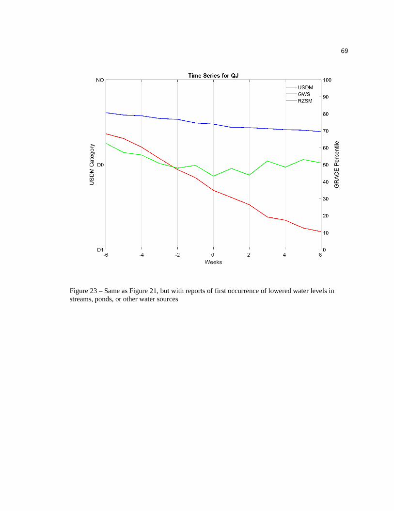
69
Figure 23 – Same as Figure 21, but with reports of first occurrence of lowered water levels in
streams, ponds, or other water sources

70
CHAPTER 4 – DISCUSSION
4.1 Groundwater Well Comparison
The overall poor correlations for the well-GRACE comparisons indicates that
GRACE GWS does not accurately reflect historic groundwater levels at this spatial
resolution. This comparison and interpreting the results from both data sources is
challenging because of the different timeframes each dataset used. Because the GRACE
data assimilation uses the Catchment LSM and ranks current GWS percentiles based on
the 1948-2009 levels, the historic data record is much longer than the well level period of
record. A few USGS wells had historic records going back into the 1970’s, but on
average they started in the 1990’s. The RTMN had even shorter periods of record,
starting around 2009, which severely limits their historic rank accuracy. However, it
seems that period of record does not determine correlation strength as demonstrated in
Figure 24. Even wells with short histories may have strong negative correlations
(negative in this comparison would indicate the same trend), and correlation strength is
highly variable with record length. Even with these limitations, the dramatic variability in
correlation values from well to well, indicates that there is some information contained
within GRACE GWS, but it does not represent local, point-based well levels. One reason
for this difference may be the differing spatial scales. Well observations are point
measurements, while GRACE GWS is a single value over 190 km2 area. The GRACE
values representing an area averaged value may not always reflect the local well
observations. Some wells have strong enough correlations to be considered significantly
different than zero – agreeing with the conclusion that there is good information

71
contained within the GRACE dataset. Even if the percentiles were off, the increasing or
decreasing trend would allow for stronger correlations than were observed.
Figure 24 – Individual well correlation values and their respective periods of record for both
USGS (red circle) and RTMN (blue triangle) well datasets.
Additionally, correlations between well levels (converted to USDM drought
levels using the percentiles in Table 2) showed weak or negative correlations with USDM
drought levels. This result was just a simple comparison that did not take into account the
potential time-lag between GWS and USDM data. Because of this result, it is clear that
raw well level data, or even data converted to historic percentile, when not accounting for
time lag, is not on its own a good drought indicator. While GRACE GWS percentiles do
not accurately represent groundwater levels from a drought monitoring perspective
because it may still contain useful land surface information that correlates well to
drought.
-1
-0.8
-0.6
-0.4
-0.2
0
0.2
0.4
0.6
0.8
1
0 5 10 15 20 25 30 35 40 45
Co
rrel
atio
n
Years of Record
RTMN USGS

72
The spatial distribution of the correlations does not appear to directly correspond
to major aquifer type as the vast majority of Nebraska land is above the High Plains
aquifer, an unconsolidated sand and gravel aquifer. While many of the better (more
negative) correlations appear along the Platte River, an area with high irrigation density,
upon closer inspection the better correlations do not appear to be associated directly with
more irrigated land. Figure 25 overlays the irrigated land with the correlation values. This
irrigation dataset was produced by USGS with MODIS imagery for the year 2012 at
250m resolution (USGS, 2015). The higher density irrigation near the south-central part
of the state around the Platte River does see good correlations, however, in other areas
where there is significant irrigation, correlations are far poorer, specifically in the
southwestern corner of the state. Additionally, throughout the Sandhills, northwestern –
northern part of the state, where there is little or no irrigation, correlations range
from -.80 to 0.4.

73
Figure 25 – Spatial distribution of individual well correlation values with irrigation density
overlaid.
4.2 Spatial Correlations
4.2.1 GRACE-USDM
The conversion of GRACE percentiles into drought levels causes a significant
loss of information. The six-decimal precision of the original GRACE percentile
(accuracy not withstanding) is grouped into five categories. All the variation within
groups is lost, including all high levels of groundwater and soil moisture (no drought
corresponding to the largest percentile range) and only the transition from one category to
another is analyzed with this correlation. Using these drought levels is necessary,
however, because of the inherent uncertainty when authoring the USDM. These levels
also are triggers for certain emergency responses in the United States, such as disaster
declaration and relief funding. In addition to the loss of information from the
reclassification of GRACE data, the GRACE drought levels revealed some areas of the

74
U.S. that have never experienced less than 30% dryness in GRACE GWS and RZSM
historical data record. This led to the entire time series for pixels to be constant (-1).
Because some covariance is required to calculate correlation, these areas are filled with
NODATA values, again losing some additional information.
Overall, both GRACE GWS and RZSM showed strong, but not perfect
correlations with USDM. GWS-USDM showed a stronger relationship than RZSM,
although there was less spatial variability with RZSM-USDM. Because of the significant
and positive relationship between these GRACE products and USDM, there is valuable
drought monitoring information contained within GRACE products.
Moving from the complete time series to the seasonal comparisons, it is clear
GRACE GWS has more agreement during JJA and SON, than MAM and DJF. RZSM
performed better as a DI (higher agreement with the gold standard of drought indicators,
USDM) during JJA, but not as notable a difference as with GWS. There were also
distinct decreases in correlations over mountainous areas during winter months. This
lends itself to a hypothesis that precipitation amount and precipitation type may influence
performance of RZSM as a drought indicator. Mountainous areas also have generally
shallow, poorly characterized soil moisture and groundwater estimates which may have
led to a disconnect between GRACE products and drought characterization in these areas.
Generally individual pixel correlations for all comparisons ranged from greater
than 0.90 to just above zero, but there is certainly a spatial pattern associated with it.
Certain factors can be immediately removed as possible causes of this pattern such as
altitude, irrigation, and precipitation, because they do not follow the same patterns as

75
higher and lower correlated areas. A possible explanation for areas not experiencing
strong agreement is the previously mentioned loss of information both from no
covariance, as well as no variation within drought levels and inherent errors in the models
and observation measurements.
In the analysis of whether GRACE datasets and USDM are independent, that is,
did the Drought Monitor authors use GRACE data when deciding areas of drought, the
correlations of data only through 2012 resulted in a slightly higher average correlation
value for both GWS and RZSM. This indicates the general trend was not affected by any
use of GRACE data for USDM. The major areas where the full timespan had higher
correlations were typically those that saw extreme droughts post-2012 such as California.
This additional change in drought level provides more trends to correlate with. While the
possibility still exists that Drought Monitor authors used GRACE data, this study shows
any overall impact was generally minor and regional.
As briefly discussed with USDM data, this research did not separate drought
impacts and drought levels into “Short-term” and “Long-term”. Not distinguishing
between these time-scales does limit the conclusion of this research. Logically, long-term
drought designations would better correlate with groundwater, where short-term drought
designations would correlate higher with soil moisture.
4.2.2 GRACE – SPI
The comparison of different accumulation periods of SPI and GRACE GWS and
RZSM indicated a logical increase of correlation as the accumulation period increased up

76
to a maximum, for GWS up to 0.543 and for RZSM up to 0.585. GWS logically takes
longer to react to precipitation changes than RZSM and shows the highest correlations
with longer accumulation periods, around 9-11 months. This timeline is in agreement
with Fiorillo et al. (2010), which states springtime river discharge is best correlated with
SPI at 9- to 12-month accumulation periods. The pattern of correlations may be explained
simply by the amount of time precipitation takes to enter groundwater. Different geologic
formations and aquifer types impact this amount of time.
RZSM shows very quick response to precipitation on the order of 2-5 months.
There is less of a spatial pattern in these comparisons, potentially due to the quicker and
more direct influence of precipitation on soil moisture. It is also important to note the
RZSM – 3-month SPI showed the highest agreement at 0.585. This very high agreement
with a well-known and widely used drought indicator shows strong promise for GRACE
RZSM as a routine drought indicator.
Seasonality of GWS-SPI comparisons show us that both DJF and JJA hold
similarly high correlations, whereas the transition seasons of MAM and SON have
slightly lower correlations. A reason these differences are not strong may be because the
minimum 9-month accumulation period obscures the original precipitation season. Liquid
precipitation would enter groundwater faster than frozen, but the 9-month SPI will allow
for seasonal frozen precipitation to melt and enter the groundwater system.
RZSM-SPI seasonal comparisons show significantly more seasonality with JJA
agreeing most strongly with 2-5-month SPI. Because frozen precipitation takes longer to
impact soil moisture than liquid precipitation, the winter DJF months have lower

77
correlations. The spatial pattern is also consistent with this precipitation type theory, and
DJF months show near zero or even slightly negative correlations over the high Rocky
Mountains at all four accumulation periods.
4.2.3 GRACE – NLDAS
The three NLDAS model comparisons showed significant agreement with
GRACE RZSM. As these comparisons are simply assessing where/when similar LSMs
produce the same trends, the resulting high correlations were mostly expected.
Differences that appeared mostly in the western U.S. could be a result of different
topographic calculations between the Catchment LSM and NLDAS LSMs. Possible
explanations could be rock/aquifer type or different observation densities. While the
patterns also do not strictly match U.S. aquifers, the different physical characteristics of
those aquifers may have a significant impact on the remote sensing and modeling aspect
of GRACE data. Additionally, because this dataset is an LSM with extra data assimilated,
the Catchment LSM may have observing or modeling bias in certain regions or may
perform better with certain precipitation types.
The warmer months of JJA and SON produced the highest correlations in all three
models. An explanation similar with the SPI correlations could also be at play here, that
is, frozen precipitation. These NLDAS models may parameterize the melting and
infiltration of snow differently to Catchment, so areas with high amounts of snow,
specifically in winter months would have less overall agreement.

78
4.3 2016 Northern Plains Flash Drought
The examination of this specific flash drought event through the perspective of
stakeholders in the region provides impact-based timelines of events that were compared
to GRACE drought products. The ability of these products to match stakeholder
observations, as well as other drought indicators such as USDM, should be a strong basis
on which to decide what drought information to look at or include for decision makers.
The survey responses revealed this drought was comprised of a rapid decrease in
both topsoil and subsoil moisture, increasing plant stress and death, followed by lowered
water levels in ponds, streams, and wells. The USDM analysis showed many reports of
drought conditions occurred near the time those areas were put into D0 or higher drought
conditions. Several months saw a large number of reports early in the season before any
widespread drought had reached those areas in the USDM. So, on monthly or longer
time-scales, USDM and stakeholder reports generally agreed, the first occurrence of
drought conditions were almost always preceding any USDM drought classification. In
this region, drought is a typical part of the climate, and dryness happens relatively often.
Based on the USDM drought percentile classifications, certain drought conditions, such
as decreased soil moisture may appear before the “historic” dry points are reached.
In the month-to-month analysis GRACE RZSM matched relatively well with the
USDM classifications. The overall trend into dry conditions was spatially and temporally
captured across the region. RZSM percentiles dropped below 10% across much of the

79
core drought region by the end of June, which correctly corresponds to D2 – D3 drought
severity. Stakeholder observations of decreased topsoil and subsoil moisture also agreed
with month to month GRACE RZSM decreases.
GRACE GWS proved a slowly changing indicator in this drought event.
Throughout the drought event, GWS percentiles did not change quickly by jumping from
higher percentiles one month to moderate or low percentiles the next, but instead
gradually decreased across the region over many months. Many areas, including the core
drought region, did end up with GWS percentiles near the 30% threshold for USDM D0
classification. GRACE GWS likely does not match the changes in stakeholder
observations and USDM classifications because of the short nature of this event. Even
with the generally poor performance of GWS for this specific event, the overall trend of
declining groundwater was captured, just over longer timescales. This still allows for
GWS percentiles to be used as a long-term drought indicator.
The quantitative analysis of zip code averaged drought indicator values,
surrounding the date of first occurrence for the three drought conditions revealed that
both USDM and GRACE RZSM picked up on deteriorating conditions long before the
observations. The lowering of GRACE percentiles may not reach any thresholds before
an observation was made, but the trend, if picked up by decision makers, could be used as
early warning for flash drought events. For both topsoil and subsoil moisture GRACE
RZSM shows declining trends over a month in advance and continues to deteriorate after
observations were made. These soil moisture percentiles also started relatively high, near

80
80%, and the 12 weeks of worsening conditions halved that, showing a significant
amount of dryness occurring.
A similar, but slower, trend is found with GRACE GWS percentiles. From 6
weeks prior to 6 weeks after first observations of lowered water levels, GWS continued
on a steady decline from ~80% to ~70%. This timeframe corresponded to rapid
intensification of drought as characterized by USDM. Because this slow trend was
relatively weak, its use as a way to pinpoint drought areas is lessened.

81
CHAPTER 5 – CONCLUSIONS
This research used several comparison methods with observed, modeled,
surveyed and professionally authored data to compare to GRACE GWS and RZSM
percentile maps. In general, GRACE data showed some correlation with these datasets,
meaning GRACE contains drought information and can provide necessary and timely
information to decision makers about drought onset and severity.
The observed well data of USGS and RTMN compared relatively poorly with
GWS, showing an expected average negative, but highly variable correlation [-0.826 < r
< 0.696]. This result coupled with previous studies of larger scale resolution GRACE
data (Zaitchik et al. 2008, Houborg et al. 2012) conclude historic GRACE GWS
percentiles are far from perfect accuracy. These poor correlations with observed data may
be explained by variable geologic and hydrologic formations, different densities in model
observation data assimilation, as well as general inaccuracies in model parameters that
determine groundwater levels.
Through the raster correlation comparisons, it was clear both GWS and RZSM
data contain drought information also found in other DI datasets. Averaged over CONUS,
correlations were positive, indicating good agreement, and significantly different than
zero. Many times, these correlations had a spatial and seasonal pattern that likely results
from how the different compared datasets deal with precipitation and groundwater
infiltration. Seasonality could also come into play when decision makers are using these
data, potentially putting more trust during the summer, JJA season, where agreement was
higher.

82
By comparing to stakeholder observations during a flash drought event, it was
found that GRACE RZSM provides a very similar picture of drought conditions and
drought levels as determined by USDM. Additionally, RZSM can provide early warning
to quick onset droughts if the data is presented in graphical form. GRACE GWS
successfully signaled lowering of water levels during this drought event, but the spatial
and graphical patterns were slow and limited for quick onset decisions. The GWS levels
respond better and would be more useful in determining the extent and severity of longer
duration drought events.
Through remote sensing data assimilation and modeling, GRACE GWS and
RZSM percentiles have proven to be useful drought indicators and tools that can benefit
stakeholders and decision makers by providing, weekly, regional scale maps of soil
moisture and groundwater trends.
5.1 Future Work
There are several areas where future work regarding the GRACE percentile
products should be considered. First, this study only assessed the accuracy of the GWS
percentile products and evaluating the accuracy of the RZSM percentiles is equally
important. Using regional, temporally continuous soil moisture networks, one can
compare observed data to GRACE percentiles to determine if the trends match. Another
area to further research is determining if aquifer type has an effect on GWS product
accuracy. This study did not separate confined and unconfined aquifers due to low
sample size, but any significant differences in accuracy found could help determine
where GRACE GWS estimates are more accurate.

83
Finally, another topic to investigate further would be the disagreement between
GRACE RZSM and NLDAS soil moisture, specifically over the Rocky Mountains. As
previously discussed, GRACE gravity data is the only observational forcing difference
between the NLDAS and Catchment LSMs, so it is possible this additional data
assimilation may be resulting in more accurate soil moisture estimates. However, in order
to determine if they are indeed more accurate, in situ soil moisture observations in that
region will nee to be collected and compared to both NLDAS and GRACE soil moisture
data. A significant improvement in soil moisture estimates would help stakeholders and
decision makers in those regions to work with the most accurate data available.

84
References
Alley, W. M. (1984). The Palmer drought severity index: limitations and assumptions.
Journal of climate and applied meteorology, 23, 1100-1109.
Brown, J. F., Wardlow, B. D., Tadesse, T., Hayes, M. J., & Reed, B. C. (2008). The
Vegetation Drought Response Index (VegDRI): A new integrated approach for
monitoring drought stress in vegetation. GIScience & Remote Sensing, 45, 16-46.
Croux, C., & Dehon, C. (2010). Influence functions of the Spearman and Kendall
correlation measures. Statistical methods & applications, 19, 497-515.
Denmead, O. T., & Shaw, R. H. (1962). Availability of Soil Water to Plants as Affected
by Soil Moisture Content and Meteorological Conditions 1. Agronomy journal,
54, 385-390.
Dillman, D. A., Phelps, G., Tortora, R., Swift, K., Kohrell, J., Berck, J., & Messer, B. L.
(2009). Response rate and measurement differences in mixed-mode surveys using
mail, telephone, interactive voice response (IVR) and the Internet. Social science
research, 38, 1-18.
Ducharne, A., Koster, R. D., Suarez, M. J., Stieglitz, M., & Kumar, P. (2000). A
catchment-based approach to modeling land surface processes in a general
circulation model: 2. Parameter estimation and model demonstration. Journal of
Geophysical Research: Atmospheres, 105, 24823-24838.
Fiorillo, F., & Guadagno, F. M. (2010). Karst spring discharges analysis in relation to
drought periods, using the SPI. Water resources management, 24, 1867-1884.
Forman, B. A., Reichle, R. H., & Rodell, M. (2012). Assimilation of terrestrial water
storage from GRACE in a snow-dominated basin. Water Resources Research, 48.
Heim Jr, R. R. (2002). A review of twentieth-century drought indices used in the United
States. Bulletin of the American Meteorological Society, 83, 1149-1165.
Houborg, R., Rodell, M., Li, B., Reichle, R., & Zaitchik, B. F. (2012). Drought indicators
based on model-assimilated Gravity Recovery and Climate Experiment (GRACE)
terrestrial water storage observations. Water Resources Research, 48.
Koster, R. D., & Suarez, M. J. (1992). Modeling the land surface boundary in climate
models as a composite of independent vegetation stands. Journal of Geophysical
Research: Atmospheres, 97, 2697-2715.
Koster, R. D., Suarez, M. J., Ducharne, A., Stieglitz, M., & Kumar, P. (2000). A
catchment-based approach to modeling land surface processes in a general

85
circulation model: 1. Model structure. Journal of Geophysical Research:
Atmospheres, 105, 24809-24822.
Kumar, S. V., Zaitchik, B. F., Peters-Lidard, C. D., Rodell, M., Reichle, R., Li, B., . . .
others. (2016). Assimilation of gridded GRACE terrestrial water storage estimates
in the North American Land Data Assimilation System. Journal of
Hydrometeorology, 17, 1951-1972.
Liang, X., Wood, E. F., & Lettenmaier, D. P. (1996). Surface soil moisture
parameterization of the VIC-2L model: Evaluation and modification. Global and
Planetary Change, 13, 195-206.
McKee, T. B., Doesken, N. J., Kleist, J., & others. (1993). The relationship of drought
frequency and duration to time scales. Proceedings of the 8th Conference on
Applied Climatology, 17, pp. 179-183.
Mitchell, K. E., Lohmann, D., Houser, P. R., Wood, E. F., Schaake, J. C., Robock, A., . . .
others. (2004). The multi-institution North American Land Data Assimilation
System (NLDAS): Utilizing multiple GCIP products and partners in a continental
distributed hydrological modeling system. Journal of Geophysical Research:
Atmospheres, 109.
Niu, G.-Y., Seo, K.-W., Yang, Z.-L., Wilson, C., Su, H., Chen, J., & Rodell, M. (2007).
Retrieving snow mass from GRACE terrestrial water storage change with a land
surface model. Geophysical Research Letters, 34.
Niu, G.-Y., Yang, Z.-L., Mitchell, K. E., Chen, F., Ek, M. B., Barlage, M., . . . others.
(2011). The community Noah land surface model with multiparameterization
options (Noah-MP): 1. Model description and evaluation with local-scale
measurements. Journal of Geophysical Research: Atmospheres, 116.
Otkin, J. A., Anderson, M. C., Hain, C., Mladenova, I. E., Basara, J. B., & Svoboda, M.
(2013). Examining rapid onset drought development using the thermal infrared--
based evaporative stress index. Journal of Hydrometeorology, 14, 1057-1074.
Palmer, C. W. (1965). Meteorological drought. US Weather Bureau research paper.
Rodell, M., Chen, J., Kato, H., Famiglietti, J. S., Nigro, J., & Wilson, C. R. (2007).
Estimating groundwater storage changes in the Mississippi River basin (USA)
using GRACE. Hydrogeology Journal, 15, 159-166.
Rouse Jr, J. W., Haas, R. H., Schell, J. A., & Deering, D. W. (1974). Monitoring
vegetation systems in the Great Plains with ERTS.
Rowlands, D. D., Luthcke, S. B., Klosko, S. M., Lemoine, F. G., Chinn, D. S., McCarthy,
J. J., . . . Anderson, O. B. (2005). Resolving mass flux at high spatial and temporal

86
resolution using GRACE intersatellite measurements. Geophysical Research
Letters, 32.
Smith, A. B., & Katz, R. W. (2013). US billion-dollar weather and climate disasters: data
sources, trends, accuracy and biases. Natural hazards, 67, 387-410.
Su, H., Yang, Z.-L., Dickinson, R. E., Wilson, C. R., & Niu, G.-Y. (2010). Multisensor
snow data assimilation at the continental scale: The value of Gravity Recovery
and Climate Experiment terrestrial water storage information. Journal of
Geophysical Research: Atmospheres, 115.
Svoboda, M., LeComte, D., Hayes, M., Heim, R., Gleason, K., Angel, J., . . . others.
(2002). The drought monitor. Bulletin of the American Meteorological Society,
83, 1181-1190.
Tallaksen, L. M., & Van Lanen, H. A. (2004). Hydrological drought: processes and
estimation methods for streamflow and groundwater (Vol. 48). Elsevier.
Tapley, B. D., Bettadpur, S., Watkins, M., & Reigber, C. (2004). The gravity recovery
and climate experiment: Mission overview and early results. Geophysical
Research Letters, 31.
United States Drought Monitor (2016, 6). The United States Drought Monitor.
United States Geological Survey (2015, 4). The 2012 Moderate Resolution Imaging
Spectroradiometer (MODIS) Irrigated Agriculture 250-Meter Dataset for the
Conterminous United States (MIrAD-US). Retrieved from
https://earlywarning.usgs.gov/USirrigation
University of Nebraska-Lincoln Institute of Agriculture & Natural Resources (2017).
Nebraska Real-Time Monitoring Network.
Wahr, J., Molenaar, M., & Bryan, F. (1998). Time variability of the Earth's gravity field:
Hydrological and oceanic effects and their possible detection using GRACE.
Journal of Geophysical Research: Solid Earth, 103, 30205-30229.
Wilhite, D. A. (2000). Drought as a natural hazard: concepts and definitions.
Wilhite, D. A., & Glantz, M. H. (1985). Understanding: the drought phenomenon: the
role of definitions. Water international, 10, 111-120.
World Meteorological Organization (2012). Standardized Precipitation Index User Guide
(M. Svoboda, M. Hayes and D. Wood). Geneva.
Xia, Y., Ek, M., Wei, H., & Meng, J. (2012). Comparative analysis of relationships
between NLDAS-2 forcings and model outputs. Hydrological Processes, 26, 467-
474.

87
Xia, Y., Mitchell, K., Ek, M., Cosgrove, B., Sheffield, J., Luo, L., . . . others. (2012).
Continental-scale water and energy flux analysis and validation for North
American Land Data Assimilation System project phase 2 (NLDAS-2): 2.
Validation of model-simulated streamflow. Journal of Geophysical Research:
Atmospheres, 117.
Yeh, P. J.-F., Swenson, S. C., Famiglietti, J. S., & Rodell, M. (2006). Remote sensing of
groundwater storage changes in Illinois using the Gravity Recovery and Climate
Experiment (GRACE). Water Resources Research, 42.
Zaitchik, B. F., Rodell, M., & Reichle, R. H. (2008). Assimilation of GRACE terrestrial
water storage data into a land surface model: Results for the Mississippi River
basin. Journal of Hydrometeorology, 9, 535-548.

88
Appendix I

89

90

91

92

93

94

95

96

97

98

99

100

101

102
103

104
Appendix II
# ##
# Description: R code to calculate correlation coefficients between well and GRACE data
# Author: Anthony Mucia
# Date: May 2018
# Notes: Very basic table output, which is then manually transformed into useable
formats
# to speed up
# ##
.libPaths("/Library/Path")
library(tidyverse)
## Reading in Data
USGSPerc <- read_csv("/Path/To/Data/USGSWellPercentiles.csv", na = "NA")
USGSWellDM <- read_csv("/Path/To/Data/USGSWellDM.csv", na = "NA")
graceUSGSPerc <- read_csv("/Path/To/Data/USGSGRACEPercentiles.csv", na = "NA")
graceUSGSPercC <- read_csv("/Path/To/Data/USGSGRACE_C_Percentiles.csv", na =
"NA")
USGSDM <- read_csv("/Path/To/Data/USGSDM.csv", na = "NA")
RTMNPerc <- read_csv("/Path/To/Data/RTMNWellPercentiles.csv", na = "NA")
RTMNWellDM <- read_csv("/Path/To/Data/RTMNWellDM.csv", na ="NA")
graceRTMNPerc <- read_csv("/Path/To/Data/RTMNGRACEPercentiles.csv", na =
"NA")
graceRTMNPercC <- read_csv("/Path/To/Data/RTMNGRACE_C_Percentiles.csv", na =
"NA")
RTMNDM <- read_csv("/Path/To/Data/RTMNDM.csv", na = "NA")
USGScols <- ncol(USGSPerc)
RTMNcols <- ncol(RTMNPerc)
usgscor <- 0
rtmncor <- 0
## Setting up column naming
for (i in 2:USGScols){
names(usgscor[i]) <- names(USGSPerc[i])
}
for (i in 2:RTMNcols){
names(rtmncor[i]) <- names(RTMNPerc[i])
}
as.data.frame(usgscor)
as.data.frame(rtmncor)
names(usgscor) <- names(USGSPerc)

105
names(rtmncor) <- names(RTMNPerc)
## Percentile - Percentile Correlation Calculations
for (i in 2:USGScols){
usgscor[i] <- cor.test(USGSPerc[[i]], graceUSGSPerc[[i]], use =
"pairwise.complete.obs", method = "spearman")
}
for(i in 2:RTMNcols){
rtmncor[i] <- cor(RTMNPerc[[i]], graceRTMNPerc[[i]], use = "pairwise.complete.obs",
method = "spearman")
}
write.table(usgscor, "/Path/To/Data/Out/usgsCor.csv", sep = ",", append = T)
write.table(rtmncor, "/Path/To/Data/Out/rtmnCor.csv", sep = ",", append = T)
## Percentile - Cubic Correlations
for (i in 2:USGScols){
usgscor[i] <- cor(USGSPerc[[i]], graceUSGSPercC[[i]], use = "pairwise.complete.obs",
method = "spearman")
}
for(i in 2:RTMNcols){
rtmncor[i] <- cor(RTMNPerc[[i]], graceRTMNPercC[[i]], use =
"pairwise.complete.obs", method = "spearman")
}
write.table(usgscor, "/Path/To/Data/Out/usgsCor.csv", sep = ",", append = T)
write.table(rtmncor, "/Path/To/Data/Out/rtmnCor.csv", sep = ",", append = T)
## Well DM Level - DM Level
for (i in 2:USGScols){
usgscor[i] <- cor(USGSWellDM[[i]], USGSDM[[i]], use = "pairwise.complete.obs",
method = "spearman")
}
for(i in 2:RTMNcols){
rtmncor[i] <- cor(RTMNWellDM[[i]], RTMNDM[[i]], use = "pairwise.complete.obs",
method = "spearman")
}
write.table(usgscor, "/Path/To/Data/Out/usgsCor.csv", sep = ",", append = T)
write.table(rtmncor, "/Path/To/Data/Out/rtmnCor.csv", sep = ",", append = T)

106
Appendix III
# ##
# Description: Python code to calculate correlation coefficients between two raster
datasets
# Author: Anthony Mucia
# Date: May 2018
# Notes: This code is based around a community answer by ESRI Community user
Xander Bakker
# https://community.esri.com/thread/200534-re-correlation-between-two-different-
rasters
# ##
def main():
import arcpy, glob, winsound, os
import numpy as np
import numpy.ma as ma
import pandas as pd arcpy.env.overwriteOutput = True
dataPath1 = r'Input/Data_1/Folder'
dataPath2 = r'Input/Data_2/Folder'
L1 = glob.glob(dataPath1+'\*.tif')
L2 = glob.glob(dataPath2+'\*.tif')
nodata = -999
out_ras = r'Output/Raster/Folder/output.tif'
outDataPath = r'Output/Raster/Folder/'
print(" List 1 Raster Count = "+str(len(L1)))
print(" List 2 Raster Count = "+str(len(L2)))
L1 = sorted(L1)
L2 = sorted(L2)
print "Creating arrays..."
lst_np_ras = []
for i in range(0, len(L1)):
ras_path1 = L1[i]
print " - ", ras_path1
ras_np1 = arcpy.RasterToNumPyArray(ras_path1)
ras_path2 = L2[i]
print " - ", ras_path2
ras_np2 = arcpy.RasterToNumPyArray(ras_path2)
lst_np_ras.append([ras_np1, ras_np2])
print "Reading numPy rasters..."
ras_np = lst_np_ras[0][0]
rows = ras_np.shape[0]

107
cols = ras_np.shape[1]
print " - rows:", rows
print " - cols:", cols
print "Creating output numPy array..."
ras_path = L1[0]
raster = arcpy.Raster(ras_path)
ras_np_res = np.ndarray((rows, cols))
ras_np_res2 = np.ndarray((rows, cols))
print " - rows:", ras_np_res.shape[0]
print " - cols:", ras_np_res.shape[1]
print "Looping through pixels..."
pix_cnt = 0
for row in range(rows):
for col in range(cols):
pix_cnt += 1
if pix_cnt % 5000 == 0:
print " - row:", row, " col:", col, " pixel:", pix_cnt
lst_vals1 = []
lst_vals2 = []
try:
for lst_pars in lst_np_ras:
lst_vals1.append(lst_pars[0][row, col])
lst_vals2.append(lst_pars[1][row, col])
lst_vals1 = ReplaceNoData(lst_vals1, nodata)
lst_vals2 = ReplaceNoData(lst_vals2, nodata)
correlation = SpearmanCorrelation(lst_vals1, lst_vals2, nodata)
ras_np_res[row, col] = correlation
except Exception as e:
print "ERR:", e
print " - row:", row, " col:", col, " pixel:", pix_cnt
print " - lst_vals1:", lst_vals1
print " - lst_vals2:", lst_vals2
pnt = arcpy.Point(raster.extent.XMin, raster.extent.YMin)
xcellsize = raster.meanCellWidth
ycellsize = raster.meanCellHeight
dsc = arcpy.Describe(L1[0])
coord_sys = dsc.spatialReference
print "Writing output raster..."
print " - ", out_ras
ras_res = arcpy.NumPyArrayToRaster(ras_np_res, lower_left_corner=pnt,
x_cell_size=xcellsize,

108
y_cell_size=ycellsize, value_to_nodata=nodata)
ras_res.save(out_ras)
arcpy.DefineProjection_management(in_dataset=out_ras, coor_system=coord_sys)
print("Cleaning up work files...")
FileCleanup(outDataPath)
print ("Complete")
def FileCleanup(path):
import os, glob, winsound
file_name = os.listdir(path)
for item in file_name:
if item.endswith(".xml") or item.endswith(".tfw") or item.endswith(".ovr"):
os.remove(os.path.join(path, item))
winsound.Beep(1000,1000)
def PearsonCorrelation(a, b, nodata):
import numpy try:
coef = numpy.corrcoef(a,b)
return coef[0][1]
except:
return nodata
def SpearmanCorrelation(a, b, nodata):
import pandas as pd try:
a = pd.Series(a)
b = pd.Series(b)
coef = a.corr(b,method = "spearman")
return coef
except:
return nodata
def ReplaceNoData(lst, nodata):
res = []
for a in lst:
if a == nodata:
res.append(None)
else:
res.append(a)
return res
if __name__ == '__main__':
main()


![Time&variable gravity from GRACE: First resultsgeoid.colorado.edu/grace/docs/GRL-WahrSwenson2004.pdf2003 GRACE solution, and the static gravity field EGM96 [Lemoine et al., 1998] -](https://img.pdfslide.us/doc/110x75/6003cdbfe6f4526fff0dd2a1/timevariable-gravity-from-grace-first-2003-grace-solution-and-the-static.jpg)