ANALYSIS OF FOULING RATE AND PROPENSITY FOR … · Background of HTRI Fouling Research In 1996, HTRI constructed ... Determining the initial fouling rate This paper uses data from

ANALYSIS OF FOULING RATE AND PROPENSITY FOR EIGHT CRUDE OIL SAMPLES IN ANNULAR TEST SECTION

A. D. Smith

Heat Transfer Research, Inc. 150 Venture Drive, College Station, TX USA 77845

[email protected]

ABSTRACT Fouling data from eight crude oils were analyzed to determine the threshold wall temperature and activation energy, which are measures of fouling propensity. Tests were performed in a High Temperature Fouling Unit (HTFU) that consists of a recirculating flow loop with annular test sections. Tests were performed under initial wall temperatures (114 to 515 °C) and velocities (0.6 to 2.5 m/s) that simulate conditions in a crude oil refinery preheat train. To suppress boiling, unit was pressurized to 500–850 psig using N2. Interpretation of the data is challenging due to operation and design issues. Mathematical techniques were developed to discard data, determine the initial reference temperature, and determine the initial fouling rate. The threshold wall temperature and activation energy were determined from a linear regression of the natural logarithm of the initial fouling rate versus reciprocal absolute wall temperature.

San Joaquin Valley crude oil had the lowest fouling propensity, while Grangemouth crude oil had the highest. Fouling propensity is compared with chemical property data. INTRODUCTION Background of HTRI Fouling Research In 1996, HTRI constructed the HTFU, which was equipped with an annular fouling test section. From 1996 – 2002, the annular test section was used to evaluate crudes discussed in this paper. Since 2002, the HTFU has been redesigned and equipped with a tubular test section. This paper is the third analysis of the HTFU annular test section data. Bennett and Palen (2003) performed a broad analysis investigating trends across different crudes, such as general trends with initial wall temperature, velocity, and colloidal instability index. Malayeri and Müller-Steinhagen (2011) used the data to demonstrate that an artificial neural network (ANN) can predict fouling. Their report focused on the ANN method and did not present fouling propensity results for each crude. This paper

demonstrates how criteria-based methods may be used to reduce the data and measure fouling propensity. Research Objectives Improved data reduction methods. Good experimental research depends on both the quality of the measurements and the data analysis methods. HTRI has identified three key facets of fouling analysis and proposes objective mathematical techniques for each:

1. Discarding data 2. Identifying the t=0 reference point that is used to

calculate the fouling resistance 3. Determining the initial fouling rate

This paper uses data from HTRI’s HTFU annular test section to demonstrate improved data reduction techniques and illustrate how fouling threshold data may be used to rank fouling propensity. Fouling threshold to rank fouling propensity. The ability to rate the fouling propensity of a crude is valuable to refiners because it influences operating guidelines and the processing cost of the crude (Wiehe, 2008). Typically, fouling propensity is gauged through chemical analysis. For example, asphaltene content, colloidal instability index (CII), or compatibility/blending numbers are used as general indicators of the likelihood of a crude to foul but do not guarantee fouling behavior. This paper demonstrates that the HTFU is capable of measuring the fouling propensity of a crude, which is quantified by the threshold wall temperature (temperature at which significant fouling occurs) and activation energy (a metric of temperature sensitivity). TEST METHODS HTFU Annular Test Section The HTFU process flow diagram is shown in Fig. 1. The HTFU has a total crude charge of 30 L. The crude is recirculated through two parallel annular fouling test sections. Because the fluid is shared, the bulk temperature

Proceedings of International Conference on Heat Exchanger Fouling and Cleaning - 2013 (Peer-reviewed) June 09 - 14, 2013, Budapest, Hungary Editors: M.R. Malayeri, H. Müller-Steinhagen and A.P. Watkinson

Published online www.heatexchanger-fouling.com

1

and pressure are the same for each test section. The velocity and power (wall temperature) are independently controlled. The dimensions and design of the annular test section are shown in Fig. 2. A cylindrical cartridge heater probe is centered along the length. Four thermocouples are placed underneath the outer sheath at 90-degree offsets. The probes are removable. More than 80 percent of the tests were performed with unpolished stainless steel probes; however, carbon steel, stainless steel low-fin, and polished stainless steel probes were also used. Table 1 summarizes the range of operating parameters evaluated. For each run, constant duty, nominal velocity, and bulk temperature were maintained. The data acquisition system recorded the following:

power to heating elements runtime inlet and outlet bulk temperatures pressure drop across a Venturi flow meter system pressure wall temperature of the fouling probe at the four

circumferentially spaced measurement points

Table 1. Range of HTFU operating parameters evaluated for annular test section Parameter Range tested

Power 175 – 2300 W Velocity Shear stress

0.5 – 2.5 m/s 0.7 – 15 Pa

Bulk temperature 40 – 300 °C Wall temperature 114 – 515 °C Pressure 500 – 850 psig

TCP

Hot crude oilreservoir

TCTC

TC

Te

st s

ectio

n 1

Te

st s

ect

ion

2

VenturiFlow meter

VenturiFlow meter

Circulationpump

Pressure relief valve

Vent

Nitrogen

P Pressure Gauge

TC Thermocouple

TCP

Hot crude oilreservoir

TCTC

TC

Te

st s

ectio

n 1

Te

st s

ect

ion

2

VenturiFlow meter

VenturiFlow meter

Circulationpump

Pressure relief valve

Vent

Nitrogen

P Pressure Gauge

TC Thermocouple

Fig. 1. HTFU process and instrumentation diagram

Operational and Design Issues There were several operational and design issues with the HTFU during this early test program. Operational issues.

Runs usually lasted between 12 hours and 1 week, with some lasting only a few hours. It is unreliable to conclude low or minimal fouling from short duration tests; it is possible that the fouling had not proceeded beyond induction.

Protracted start-up times made it unreasonable to collect all transient data. Currently available data does not include data prior to t=0, thus it is not possible to scrutinize the selection of the t=0 reference point.

Inconsistent cleaning procedures (Bennett, 2006) may make it difficult to compare data from subsequent runs on the same test section.

Fig. 2. Annular test section Design issues.

Unit operated outside and bulk temperatures sometimes correlated with weather and day-night temperature fluctuations. The control system in this

Heater Rod Cross Section

Hea

ter

Flow inCentering bore14.3mm

Flow out

Outlet pipe 41.275mm

Heater cord

152.

4 m

m

Thermocouple tips 4 @ 90 degrees

Bulk outlet thermocouple

Bulk inlet thermocouple17

1.4

mm

Inlet pipe 38.1mm

Centered annular rod 12.7 mm OD SS tube

34.3 mm OD, 18.2 mm ID, SS tube

Boundary layer trip

Cartridgeheater

6.35 mm

Welded 304 SS tubing

Magnesium

76.2

mm

Smith / Analysis of fouling rate and propensity for eight crude oil samples …

www.heatexchanger-fouling.com 2

early design could not compensate for these variations.

Calibration constants for the test probe changed over time (Bennett, 2007b), which may be attributed to manufacturing quality assurance.

Flow in the test section was underdeveloped and asymmetrical. Bennett (2007b) used a computational fluid dynamics (CFD) model to show that fluid velocity in the annulus varied from 0.5 – 1.3 m/s as a function of circumferential position.

Because of these issues, a higher-than-desired amount of noise exists in the data. Despite this noise, much can be learned by analyzing trends across the data as a whole.

DATA REDUCTION METHODS Methods to reconcile data and establish key performance parameters consist of the following: Initial Screening of Data

Because the goal of this study is to use HTFU data to rank the fouling propensity of crudes, analysis was restricted to runs using a smooth stainless steel heater probe (> 80% of runs) and bulk temperatures between 232 – 288 °C (~70% of runs). This initial screen reduces the data set from 15 crudes (237 runs) to 10 crudes (139 runs). Of the 10 crudes, only eight had enough data points to evaluate fouling propensity.

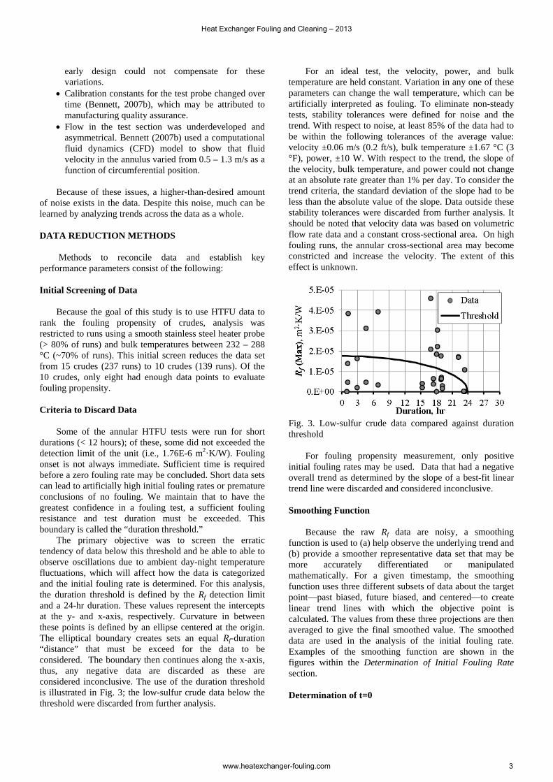
Criteria to Discard Data Some of the annular HTFU tests were run for short durations (< 12 hours); of these, some did not exceeded the detection limit of the unit (i.e., 1.76E-6 m2·K/W). Fouling onset is not always immediate. Sufficient time is required before a zero fouling rate may be concluded. Short data sets can lead to artificially high initial fouling rates or premature conclusions of no fouling. We maintain that to have the greatest confidence in a fouling test, a sufficient fouling resistance and test duration must be exceeded. This boundary is called the “duration threshold.” The primary objective was to screen the erratic tendency of data below this threshold and be able to able to observe oscillations due to ambient day-night temperature fluctuations, which will affect how the data is categorized and the initial fouling rate is determined. For this analysis, the duration threshold is defined by the Rf detection limit and a 24-hr duration. These values represent the intercepts at the y- and x-axis, respectively. Curvature in between these points is defined by an ellipse centered at the origin. The elliptical boundary creates sets an equal Rf-duration “distance” that must be exceed for the data to be considered. The boundary then continues along the x-axis, thus, any negative data are discarded as these are considered inconclusive. The use of the duration threshold is illustrated in Fig. 3; the low-sulfur crude data below the threshold were discarded from further analysis.

For an ideal test, the velocity, power, and bulk temperature are held constant. Variation in any one of these parameters can change the wall temperature, which can be artificially interpreted as fouling. To eliminate non-steady tests, stability tolerances were defined for noise and the trend. With respect to noise, at least 85% of the data had to be within the following tolerances of the average value: velocity ±0.06 m/s (0.2 ft/s), bulk temperature ±1.67 °C (3 °F), power, ±10 W. With respect to the trend, the slope of the velocity, bulk temperature, and power could not change at an absolute rate greater than 1% per day. To consider the trend criteria, the standard deviation of the slope had to be less than the absolute value of the slope. Data outside these stability tolerances were discarded from further analysis. It should be noted that velocity data was based on volumetric flow rate data and a constant cross-sectional area. On high fouling runs, the annular cross-sectional area may become constricted and increase the velocity. The extent of this effect is unknown.

Fig. 3. Low-sulfur crude data compared against duration threshold For fouling propensity measurement, only positive initial fouling rates may be used. Data that had a negative overall trend as determined by the slope of a best-fit linear trend line were discarded and considered inconclusive. Smoothing Function Because the raw Rf data are noisy, a smoothing function is used to (a) help observe the underlying trend and (b) provide a smoother representative data set that may be more accurately differentiated or manipulated mathematically. For a given timestamp, the smoothing function uses three different subsets of data about the target point—past biased, future biased, and centered—to create linear trend lines with which the objective point is calculated. The values from these three projections are then averaged to give the final smoothed value. The smoothed data are used in the analysis of the initial fouling rate. Examples of the smoothing function are shown in the figures within the Determination of Initial Fouling Rate section.

Determination of t=0

Heat Exchanger Fouling and Cleaning – 2013


Fouling resistance is calculated from a change in wall temperature relative to the initial time zero (t=0) reference temperature. Erroneous selection of t=0 can lead to overestimated initial fouling rates if the system is still in transient start-up, or underestimated fouling rates and resistances if fouling has already begun. In an ideal fouling test, test conditions could be achieved instantly at the press of a button. Unfortunately, this is never the case because high temperatures need to be obtained in units with relatively large thermal masses; an appreciable transient is unavoidable. Conceptually, the t=0 reference point is selected at the first point at which operating parameters are at steady-state. However, in practice, t=0 was often determined in a less-than-objective manner (e.g., when the data acquisition system is turned on after the system appears stable, or by visual selection from a graph or table). Although these inspection methods are reasonable, they are subjective, not rigorous, and thereby vulnerable to inconsistent application. Further, they do not provide any metrics about start-up or the stability of the system. Such data would be very useful in (a) improving start-up procedures and (b) comparing start-up transients among runs. The first step in improving the selection of the t=0 reference is to begin data collection when heat is applied to the unit. Doing so provides a comprehensive data set for the experiment and allows t=0 to be determined during posted experiment analysis rather than in the moment of the experiment. Including the start-up transient provides greater ability to review and reanalyze the data in the future as new methods and criteria are developed. To mathematically determine the t=0 reference, we use stability criteria. From the smoothed data, the first derivative is evaluated over a period of time (e.g., 30 minutes). For each operating parameter (velocity, power, and bulk temperature), a maximum absolute rate of change is defined that is tight but reasonable for the instrumentation and controls unique to the test equipment. The first timestamp is found, at which point all operating parameters are within the tolerance rate of change (i.e., at steady state). In an analogous fashion, noise criteria may be applied as a second layer of evaluation. This technique provides a rigorous and reproducible method for determining the t=0 reference.

Determination of Initial Fouling Rate The data that remained after the initial screening and discarding steps were sorted into Tier 1 or 2 categories. Tier 1 data are “pretty data” that have smooth logical fouling resistance curves. Because of their ideal shape, the effect of external influences was not considered to be significant. Mathematically, Tier 1 data is defined by the following:

More than 50% of the fouling resistances are positive.

More than 90% of the first derivative of fouling resistances is positive.

No more than one sign changes in the first derivative. The end point has a positive fouling resistance.

There is a maximum of one change in sign of the second derivative of fouling resistance.

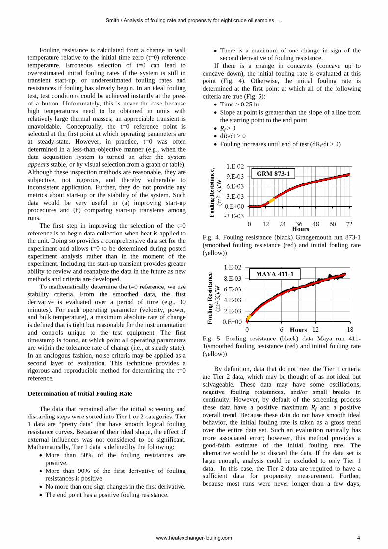
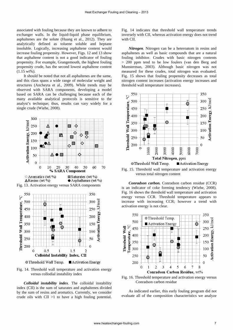
If there is a change in concavity (concave up to concave down), the initial fouling rate is evaluated at this point (Fig. 4). Otherwise, the initial fouling rate is determined at the first point at which all of the following criteria are true (Fig. 5):

Time > 0.25 hr Slope at point is greater than the slope of a line from

the starting point to the end point Rf > 0 dRf/dt > 0 Fouling increases until end of test (dRf/dt > 0)

Fig. 4. Fouling resistance (black) Grangemouth run 873-1 (smoothed fouling resistance (red) and initial fouling rate (yellow))

Fig. 5. Fouling resistance (black) data Maya run 411-1(smoothed fouling resistance (red) and initial fouling rate (yellow)) By definition, data that do not meet the Tier 1 criteria are Tier 2 data, which may be thought of as not ideal but salvageable. These data may have some oscillations, negative fouling resistances, and/or small breaks in continuity. However, by default of the screening process these data have a positive maximum Rf and a positive overall trend. Because these data do not have smooth ideal behavior, the initial fouling rate is taken as a gross trend over the entire data set. Such an evaluation naturally has more associated error; however, this method provides a good-faith estimate of the initial fouling rate. The alternative would be to discard the data. If the data set is large enough, analysis could be excluded to only Tier 1 data. In this case, the Tier 2 data are required to have a sufficient data for propensity measurement. Further, because most runs were never longer than a few days,



evaluating the initial fouling resistance over the entire data set is reasonable. Figs. 6 and 7 are examples of Tier 2 data.

Fig. 6. Fouling resistance data (black) for Arab medium run 610-1 (smoothed fouling resistance (red) and initial fouling rate (yellow))

Fig. 7. Fouling resistance data (black) for Arab medium run 604-1 (smoothed fouling resistance (red) and initial fouling rate (yellow)) FOULING PROPENSITY MEASUREMENTS With respect to wall temperatures and velocity, fouling propensity can be described by initiation, activation energy, and magnitude. The initiation of fouling may be described as a threshold curve at which fouling occurs (Knudsen et al., 1999; Panchal and Kuru, 1997; Polley et al., 2002; Yang et al., 2011). Activation energy is a metric of temperature sensitivity where lower values equal greater temperature sensitivity and thus a greater fouling propensity. Magnitude is the steady-state fouling resistance observed from a batch fouling test and would represent the total fouling potential of the crude. Because of their short duration, most runs never reached a steady-state condition; thus, evaluation of fouling magnitude is not possible. The fouling wall temperature threshold and temperature sensitivity may be determined. Trends with velocity are modest and/or are not discernible among the scatter in the data and therefore not considered in this analysis. The initial fouling rate and initial wall temperature data for each crude were plotted in an Arrehius plot as illustrated in Fig. 8 with Refinery Blend 2 crude (RB2). The activation energy is computed from the slope of the linear trend line divided by the gas constant (8.314 J/mol·K). The threshold wall temperature is the initial wall temperature at the intersection of the minimum detection rate and the linear regressed line. The minimum detectable rate for the dataset (3.9E-5 m2·K/J; ln(dRf,dt) = -10.2), which was determined by dividing the detection limit

(1.76E-5 m2·K/W) by the median duration (26.8hrs) of the data set. Regression uncertainty was used to determine the 95% confidence intervals for the respective measurements.

Fig. 8. Arrhenuis plot of RB2 fouling data RESULTS Figs. 9 and 10 rank the fouling propensity of the crudes with respect to threshold wall temperature and activation energy, respectively. Because operation at higher wall temperature is desired, a higher threshold wall temperature is the primary preference. Fig. 9 indicates that many of the crudes have similar threshold wall temperatures (ARM and RB2 are the same). To further sort these crudes, the activation energy can be considered. Fig. 11 shows the relative relationship of each crude with respect to activation energy and threshold wall temperature. From Fig. 11, the overall propensity to foul from least to greatest may be ordered as follows:

1. San Joaquin Valley (SJV) 2. Loreto (LRT) 3. Refinery Blend #2 (RB2) 4. Arab Medium (ARM) 5. Refinery Blend #1 (RB1) 6. Maya 7. Low-sulfur (LSC) 8. Grangemouth (GRM)

From Fig. 11 it is also observed that there is a strong linear relationship between activation energy and threshold wall temperature for the middle six crudes. GRM and SJV are the exceptions.

Fig. 9. Ranking of crude fouling propensity based on

threshold wall temperature



Fig. 10. Ranking of crude fouling propensity based on

activation energy

Fig. 11. Fouling propensity plot DISCUSSION HTFU With the annular test section on the HTFU, HTRI was able to collect fouling data capable of measuring the fouling propensity of crude oil samples. Since this data was collected, the HTFU has had the following upgrades to further improve its reliability (Bennett, 2007b; Huang et al., 2012):

relocation inside a climate-controlled building improved control software and hardware conversion to tubular test section with enough length

to allow fully-developed turbulent prior to entry established consistent and repeatable turnaround

protocols established protocol for beginning data collection

during transient start-up established protocol to allow test to run long enough

to either observe steady-state fouling or have confidence that no fouling would occur

Fouling Propensity and Crude Oil Chemistry Fouling unit testing is only half of the experimental effort. Understanding how the chemistry of the crude influences fouling behavior must also be characterized. The ultimate goal is to combine these data to develop a predictive model. Where chemical property data are

available, comparison can be made with fouling propensity data. During this early test program, not all chemical analyses were performed that are now considered to be indicative of fouling behavior. The following section compiles the results from above and plots the chemistry of the crudes verse the fouling propensity metrics (each data point is a single crude). Solubility classes (SARA). The composition of a crude oil sample may be characterized by the relative content of six major categories of organic compounds based on solubility: volatiles, coke, saturates, aromatics, resins, and asphaltenes. Volatiles (e.g., methane, carbon dioxide) and coke are dissolved gases and insoluble solids, respectively. Thus, they are not part of the liquid phase nor generally considered a factor in fouling behavior. The remaining four components are collectively referred to by the acronym SARA for the first letter of each class. Figs. 12 and 13 plot the threshold wall temperature and activation energy versus the SARA components. Trends with SARA components are vague at best. Saturates are hydrocarbons in which all carbon bonds are single bonds. Alkanes or aliphatic compounds (e.g., hexane and heptane) are saturates. With regard to fouling, saturates are the non-solvent phase for asphaltenes, the component largely attributed to fouling. As saturate content increases, fouling tendency increases. Aromatics are the solvent phase for asphaltenes. Increasing proportion of aromatics helps keep the asphaltenes dissolved and less likely to precipitate and adhere to the hot wall surface. Resins act as dispersants helping to maintain the colloidal stability of the dissolved asphaltenes. Of the four SARA components, the strongest trend with threshold temperature is resin content (Fig. 12)

Fig. 12. Threshold wall temperature versus SARA

components. Trend line is fit to resins data Asphaltenes are large multi-ring molecules (Bennett and Palen, 2003) and are the primary component of crude



associated with fouling because they are known to adhere to exchanger walls. In the liquid-liquid phase equilibrium, asphaltenes are the solute (Huang et al., 2012). They are analytically defined as toluene soluble and heptane insoluble. Logically, increasing asphaltene content would increase fouling propensity. However, Figs. 12 and 13 show that asphaltene content is not a good indicator of fouling propensity. For example, Grangemouth, the highest fouling propensity crude, has the second lowest asphaltene content (1.15 wt%). It should be noted that not all asphaltenes are the same, and this class spans a wide range of molecular weight and structures (Ancheyta et al., 2009). While trends may be observed with SARA components, developing a model based on SARA can be challenging because each of the many available analytical protocols is sensitive to the analyst’s technique; thus, results can vary widely for a single crude (Wiehe, 2008).

Fig. 13. Activation energy versus SARA components

Fig. 14. Threshold wall temperature and activation energy

versus collodial instability index Colloidal instability index. The colloidal instability index (CII) is the sum of saturates and asphaltenes divided by the sum of resins and aromatics. Currently, we consider crude oils with CII >1 to have a high fouling potential.

Fig. 14 indicates that threshold wall temperature trends inversely with CII, whereas activation energy does not trend with CII. Nitrogen. Nitrogen can be a heteroatom in resins and asphaltenes as well as basic compounds that are a natural fouling inhibitor. Crudes with basic nitrogen contents > 200 ppm tend to be low foulers (van den Berg and Munsterman, 2003). Although basic nitrogen was not measured for these crudes, total nitrogen was evaluated. Fig. 15 shows that fouling propensity decreases as total nitrogen content increases (activation energy increases and threshold wall temperature increases).

Fig. 15. Threshold wall temperature and activation energy

versus total nitrogen content

Conradson carbon. Conradson carbon residue (CCR) is an indicator of coke forming tendency (Wiehe, 2008). Fig. 16 shows the threshold wall temperature and activation energy versus CCR. Threshold temperature appears to increase with increasing CCR; however a trend with activation energy is not clear.

Fig. 16. Threshold temperature and activation energy versus

Conradson carbon residue As indicated earlier, this early fouling program did not evaluate all of the composition characteristics we analyze



now. Currently, we also evaluate oil compatibility, total acid number, sediment, and a variety of other elemental compositions such as H/C, oxygen, sulfur, chlorides, and metals. CONCLUSIONS 1. Mathematical methods for discarding data, determining

t=0 reference, and calculating the initial fouling rate are rigorous and reproducible. Additionally, the tolerances and thresholds used in these methods can be compared and/or standardized among fouling researchers.

2. HTRI’s HTFU is capable of characterizing the fouling propensity of crudes.

3. Fouling thresholds, activation energy, and magnitude may be used to rank crude fouling propensity. San Joaquin Valley and Grangemouth had the least and greatest fouling propensity, respectively.

4. CII alone is not a reliable indicator of fouling propensity.

5. Asphaltene content is not a good indicator of fouling propensity

6. Crude oil chemistry needs to be correlated with fouling propensity.

NOMENCLATURE CCR Conradson carbon residue CII Collodial instability index dRf/dt Fouling resistance rate, units, m2·K/(W·h) HTFU High temperature fouling unit Rf Fouling resistance, units SARA Saturates, Aromatics, Resins, and Asphaltenes t=0 time equal zero REFERENCES Bennett, C. A., and Palen, J. W., 2003, Analysis of HTRI Crude Oil Fouling Data, Report F-13, Heat Transfer Research, Inc., College Station, TX. Bennett, C. A., 2007, Crude Oil Fouling Case Study: Mechanism Identification and Mitigation, Report F-15, Heat Transfer Research, Inc., College Station, TX. Bennett, C. A., 2007, High Temperature Fouling Unit Redesign – Part I: Annular Test Section, Report F-16, Heat Transfer Research, Inc., College Station, TX. Huang, L., Farrell, K. J., and Clepper, B., 2012, Fouling Assessment of a Desalted Crude Oil, Report F-21, Heat Transfer Research, Inc., College Station, TX. Knudsen, J. G., Dahcheng, L., Ebert, W. A., 1999. The determination of the threshold fouling curve for a crude oil, Understanding Heat Exchanger Fouling and its Mitigation, eds. T. R. Bott, et al., Begell House, pp. 265-272. Malayeri, M. R., and Müller-Steinhagen, H., 2011, Neural Network Analysis of HTFU Crude Oil Fouling Database, Report F-20, Heat Transfer Research, Inc., College Station, TX. Panchal, C. B., and Kuru, W. C., 1997, Threshold conditions for crude oil fouling, Proc. Understanding Heat

Exchanger Design Fouling and Its Mitigation, Pascoli, Italy, pp. 273-780. Polley, G. T., Wilson, D. I., Yeap, B. L., and Pugh, S. J., 2002, Evaluation of laboratory crude oil threshold fouling data for application to refinery pre-heat trains, Applied Thermal Engineering, Vol. 22, pp. 777-788. van den Berg, F. G. A, and Munsterman, E. H., 2003, Feedstock effects in fouling of crude oil heat exchangers, 4th Intl. Conf. Petroleum Phase Behaviour and Fouling, Trondheim, Norway. Watkinson, A., Navaneetha-Sundaram, B., Posarac, D., 2000, Fouling of a Sweet Crude Oil Under Inert and Oxygenated Conditions, Energy Fuels, Vol. 14, pp. 64–69. Wiehe, I. A., 2008, Process Chemistry of Petroleum Macromolecules, 1st ed., CRC Press, Boca Raton, FL. Yang, M., O’meara, A., and Crittenden, B. D., 2011, Determination of crude oil fouling thresholds, Proc. Intl. Conf. Heat Exchanger Fouling and Cleaning, eds. H. Müller-Steinhagen, M. R. Malayeri, and A. P. Watkinson, Crete Island, Greece.



Documents

ANALYSIS OF FOULING RATE AND PROPENSITY FOR … · Background of HTRI Fouling Research In 1996, HTRI constructed ... Determining the initial fouling rate This paper uses data from