Ecological Economics 86 (2013) 37–46

Contents lists available at SciVerse ScienceDirect

Ecological Economics

j ourna l homepage: www.e lsev ie r .com/ locate /eco lecon

Analysis

Analysis of environmental efficiency variations: A nutrient balance approach

Viet-Ngu Hoang a,⁎, Trung Thanh Nguyen b

a Queensland University of Technology, Brisbane, Australiab Bayreuth Center of Ecology and Environmental Research, Bayreuth University, Bayreuth, Germany

⁎ Corresponding author. Tel.: +61 7 313 84325; fax:E-mail addresses: vincent.hoang@qut.edu.au (V.-N. H

thanh.nguyen@uni-bayreuth.de (T.T. Nguyen).

0921-8009/$ – see front matter © 2012 Elsevier B.V. Allhttp://dx.doi.org/10.1016/j.ecolecon.2012.10.014

a b s t r a c t

a r t i c l e i n f o

Article history:Received 12 June 2012Received in revised form 22 October 2012Accepted 23 October 2012Available online 3 December 2012

Keywords:Environmental efficiencyMaterials balanceNutrient efficiencyNutrient stochastic frontierSingle-bootstrap truncated regression

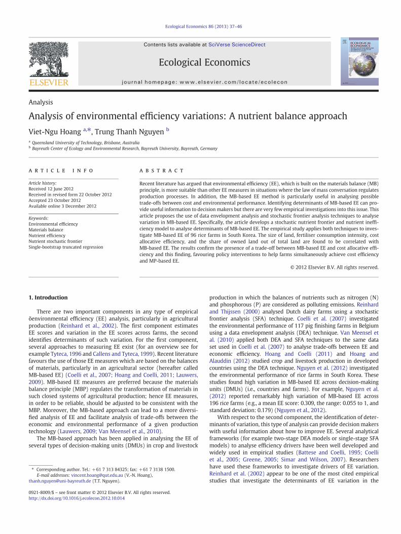
Recent literature has argued that environmental efficiency (EE), which is built on the materials balance (MB)principle, is more suitable than other EE measures in situations where the law of mass conversation regulatesproduction processes. In addition, the MB-based EE method is particularly useful in analysing possibletrade-offs between cost and environmental performance. Identifying determinants of MB-based EE can pro-vide useful information to decision makers but there are very few empirical investigations into this issue. Thisarticle proposes the use of data envelopment analysis and stochastic frontier analysis techniques to analysevariation in MB-based EE. Specifically, the article develops a stochastic nutrient frontier and nutrient ineffi-ciency model to analyse determinants of MB-based EE. The empirical study applies both techniques to inves-tigate MB-based EE of 96 rice farms in South Korea. The size of land, fertiliser consumption intensity, costallocative efficiency, and the share of owned land out of total land are found to be correlated withMB-based EE. The results confirm the presence of a trade-off between MB-based EE and cost allocative effi-ciency and this finding, favouring policy interventions to help farms simultaneously achieve cost efficiencyand MP-based EE.

© 2012 Elsevier B.V. All rights reserved.

1. Introduction

There are two important components in any type of empiricalõenvironmental efficiency (EE) analysis, particularly in agriculturalproduction (Reinhard et al., 2002). The first component estimatesEE scores and variation in the EE scores across farms, the secondidentifies determinants of such variation. For the first component,several approaches to measuring EE exist (for an overview see forexample Tyteca, 1996 and Callens and Tyteca, 1999). Recent literaturefavours the use of those EE measures which are based on the balancesof materials, particularly in an agricultural sector (hereafter calledMB-based EE) (Coelli et al., 2007; Hoang and Coelli, 2011; Lauwers,2009). MB-based EE measures are preferred because the materialsbalance principle (MBP) regulates the transformation of materials insuch closed systems of agricultural production; hence EE measures,in order to be reliable, should be adjusted to be consistent with theMBP. Moreover, the MB-based approach can lead to a more diversi-fied analysis of EE and facilitate analysis of trade-offs between theeconomic and environmental performance of a given productiontechnology (Lauwers, 2009; Van Meensel et al., 2010).

The MB-based approach has been applied in analysing the EE ofseveral types of decision-making units (DMUs) in crop and livestock

+61 7 3138 1500.oang),

rights reserved.

production in which the balances of nutrients such as nitrogen (N)and phosphorous (P) are considered as polluting emissions. Reinhardand Thijssen (2000) analysed Dutch dairy farms using a stochasticfrontier analysis (SFA) technique. Coelli et al. (2007) investigatedthe environmental performance of 117 pig finishing farms in Belgiumusing a data envelopment analysis (DEA) technique. Van Meensel etal. (2010) applied both DEA and SFA techniques to the same dataset used in Coelli et al. (2007) to analyse trade-offs between EE andeconomic efficiency. Hoang and Coelli (2011) and Hoang andAlauddin (2012) studied crop and livestock production in developedcountries using the DEA technique. Nguyen et al. (2012) investigatedthe environmental performance of rice farms in South Korea. Thesestudies found high variation in MB-based EE across decision-makingunits (DMUs) (i.e., countries and farms). For example, Nguyen et al.(2012) reported remarkably high variation of MB-based EE across196 rice farms (e.g., a mean EE score: 0.309, the range: 0.055 to 1, andstandard deviation: 0.179) (Nguyen et al., 2012).

With respect to the second component, the identification of deter-minants of variation, this type of analysis can provide decision makerswith useful information about how to improve EE. Several analyticalframeworks (for example two-stage DEA models or single-stage SFAmodels) to analyse efficiency drivers have been well developed andwidely used in empirical studies (Battese and Coelli, 1995; Coelliet al., 2005; Greene, 2005; Simar and Wilson, 2007). Researchershave used these frameworks to investigate drivers of EE variation.Reinhard et al. (2002) appear to be one of the most cited empiricalstudies that investigate the determinants of EE variation in the

1 For example, in rice production not all N and P in seed, chemical fertilisers, organicfertilisers and land are transformed into rice outputs. In fact, N and P balances, definedas the differences of the total amounts of N and P in inputs and of the total amounts ofN and P in outputs, will go to water and atmospheric environments. Scientifically,these balances have been identified as the main cause of eutrophication in lake, river,and ocean water systems (Smith et al., 1999). Therefore, in rice production, the balanceof nutrients can be considered as potential polluting agents.

38 V.-N. Hoang, T.T. Nguyen / Ecological Economics 86 (2013) 37–46

context of agricultural production; however, this study uses an EEmodel that is not adjusted for the MBP.

However, none of previous empirical studies of the MB-based EEapproach performed the second component of the analysis. Hence,it is desirable to assess critically whether the existing analyticalframeworks of analysing EE determinants can be appropriate in thecontext of MB-based EE analysis. The present article aims to fill thisgap by using bootstrap truncated two-stage DEA models proposedby Simar and Wilson (2007) and estimating the stochastic nutrientfrontier following the stochastic frontier model of Battese and Coelli(1995). Empirical applications of these models into a data set of ricefarms in South Korea also illustrated the possibility of conducting astatistical hypothesis test for trade-offs between economic andenvironmental performance.

The remainder of the article is structured as follows. Section 2 pro-vides a brief literature review on various approaches to measuringEE. Section 3 provides a mathematical illustration of the shortcomingof the EAPE model in relation to the MBP. Section 4 reviews theMB-based EE method and discusses potential uses of this methodfor trade-off and policy analysis. Section 5 introduces the use of SFAand DEA techniques to analyse variation in the MB-based EE. Section 6presents an empirical analysis of rice farms in South Korea. Section 7concludes the article.

2. Main Approaches to Measuring Environmental Efficiency:A Literature Review

Lauwers (2009) provides a review of three general groups ofmodels used to measure EE: the environmentally adjusted productionefficiency, the frontier eco-efficiency and the MB-based models. Theenvironmentally adjusted production efficiency (EAPE) uses the pro-duction frontier to analyse a relationship between inputs and outputs.In EAPE's models, pollution is viewed as either environmentally detri-mental inputs or undesirable outputs. Adding pollution as an extrainput or output in conventional productionmodels, technical efficiency(TE)measures can be estimatedwith input-oriented, output-orientatedframeworks, or with hyperbolic or directional distance functions(Chung et al., 1997; Färe et al., 1996; Färe et al., 2007; Reinhard et al.,2002). An input-orientated framework minimises inputs given fixedoutput quantities. An output-orientated frameworkmaximises outputswith fixed input quantities. The hyperbolic and directional distancefunctions allow the simultaneous expansion of outputs and the con-traction of inputs. The proponents of these methods argue that thesemodels credit farms for the contraction of pollution; therefore, TE canbe interpreted as EE.

The frontier eco-efficiency (FEE) uses the frontier framework tomodel relationships between economic and ecological outcomes toderive eco-efficiency measures (Callens and Tyteca, 1999; Tyteca,1999). The eco-efficiency measures relate the economic value of out-puts to the environmental pressures involved in production processes(Picazo-Tadeo et al., 2012). Several empirical studies have appliedthis approach (Kortelainen, 2008; Kuosmanen and Kortelainen,2005; Picazo-Tadeo et al., 2011). These applications can be seen asthe frontier operationalisation of the eco-efficiency concept in theanalysis of multidimensional sustainability (Lauwers, 2009). For ex-ample, Picazo-Tadeo et al. (2011), using a data set of 117 crop farmsin Spain, assessed the opportunities of reducing five environmentalpressures (tendency towards monoculture that has potential impactson biodiversity, N balance, P balance, energy balance, and pesticiderisks), given the value added of crop outputs.

There is a methodological distinction between EAPE and FEEmodels. The EAPE models are based on the conventional productionrelationship between inputs and outputs while the FEE models aregrounded on a hypothesised relationship between economic valuesof outputs and environmental pressures. Often they are used in dif-ferent research contexts. The primary use of the EAPE approach is to

adjust efficiency measures to account for environmental pollution inthe paradigm of costly environmental regulation. In this paradigm,efficiency analysis methods implicitly suppose that efficiency improve-ments imply cost reduction (Lauwers, 2009). The FEE approach is usedmainly to provide relative assessments among DMUs in terms of envi-ronmental performance where there are many types of environmentalpressures caused by production and consumption activities.

The third approach tomeasuring EE involves the use of theMB-basedmodels firstly proposed by Coelli et al. (2007). The MB-based modelsview pollution as the balance of materials and attempt to minimise thisbalance. The MB-based EE measures are defined as the technically fea-sible minimum materials balance to the currently observed materialsbalance. The MB-based models are distinct from the EAPE and FEEmethods because the materials balance does not appear as either aninput/output in EAPE models or an indicator of environmental pres-sures in FEE models.

Note that the MB-based and EAPE models are grounded on thesame production relationship between inputs and outputs; hencethey are very useful in analysing economic–environmental trade-offsfaced by DMUs (Lauwers, 2009; Van Meensel et al., 2010). However,the MB-based models are more suitable in situations where the MBPregulates the transformation of materials in production processes(Hoang and Alauddin, 2012; Hoang and Coelli, 2011; Nguyen et al.,2012).1 TheMB-basedmodels are preferred because given the existingconstruction of EAPE models, measuring environmental inefficiencyas the degree to which pollution (i.e., the materials balance) can bereducedwith traditional inputs and outputs held constant ismathemat-ically infeasible (Coelli et al., 2007; Hoang and Coelli, 2011; Lauwers,2009). To provide further evidence of this shortcoming of the EAPEmodels, the next section investigates the model of Reinhard et al.(2002) in which emission is modelled as an input.

3. A Major Shortcoming of the EAPE Models: A SimpleMathematical Illustration

Consider the situation where farms produce a vector of M outputs,q∈RM

þ , using a vector of K inputs, x∈RKþ. The production activity also

produces an emission of polluting substances. The amount of emis-sion is defined by the balance of nutrients:

u ¼ ax−bq ð1Þ

where a and b are the vectors representing nutrient contents of in-puts and outputs. Some inputs, such as labour and machinery, couldhave zero contents of nutrients, suggesting that vector a may includezero values.

The MBP applies to individual flows of nutrients (e.g., N or P). Insituations where there are many types of nutrients involved, onecan use weights that reflect the polluting power of different nutrientsin calculating the aggregate nutrient balance. For example, N and Pare two main causes of eutrophication (i.e. oxygen depletions causedby excessive nutrient-induced increases in the production of organicmatter) in water systems (Howarth et al., 2000). The analysis of eu-trophication requires the use of a particular set of weights that reflectthe eutrophying power of N and P in the context of a specific watersystem such that their aggregate effects can be analysed in empiricalstudies. Given an appropriate choice of N:P weights, the aggregatebalance of nutrients can be calculated. Note that the eutrophying

C

A

Iso-cost line 1

x1

x2

Iso-nutrient line

N (x1NE,,x2NE,) Iso-quant

BD

Iso-cost line 2

Fig. 1. Trade-offs between cost and environmental efficiency.

39V.-N. Hoang, T.T. Nguyen / Ecological Economics 86 (2013) 37–46

powers of N and P depend on the nature of the systems. Systems suchas lakes and rivers tend to be limited more by P than N. Furthermore,the over-enrichment of P results in a more damaging effect than theover-enrichment of N. In contrast, N is more commonly the key limitingnutrient of marine waters; thus, N levels have a greater eutrophyingpower in salt water systems than do the P levels. Hence, it is importantthat weights for N and P be carefully determined (Hoang and Coelli,2011).

Given technology with observed outputs (q) and conventional in-puts (x), one can follow the EAPE model (e.g., Reinhard et al., 2002)and define EE as the ratio of minimum feasible to the observed useof an environmentally detrimental input. This EAPE's EE measure in-volves trying to find the largest scalar, λ, such that the scaled vector( q;x;u=λ) is within the feasible production set. In this context,more environmentally efficient farms use less u. Applying this scalingto the MBP results in:

u=λ ¼ ax−bq: ð2Þ

Combining Eqs. (1) and (2), we have:

u ¼ u=λ: ð3Þ

Thus the only solution to Eq. (3) is λ ¼ 1. This solution, however,refers only to farms that are on the production frontier. Farms thatlie below the production frontier are not mathematically feasible tothe constraint of the MBP. This restriction is an undesirable feature.

In review the MB-based models is more suitable for empiricalstudies in situations where researchers believe that the MBP shouldbe applied. The next section recalls the essence of the MB-basedmodel of Coelli et al. (2007) in the context of agricultural productionwhere we are concerned with the potential polluting effects causedby the balance of nutrients.

4. The MB-based Environmental Efficiency Measure

The balance of nutrients in Eq. (1) is defined as an environmentalpressure. When outputs are fixed, the nutrient balance is minimisedwhen the total amount of nutrients in inputs (NC ¼ a′x) is minimised.Instead of minimising inputs (x), we minimise the total amount ofnutrients contained in x. In the input-orientated framework, thisapproach involves the following optimisation problem:

NC q; að Þ ¼ minx

a′x x;qh i∈Tj gn

ð4Þ

where T is a feasible production set that is defined as:

T ¼ q; xð Þ : xcanproduceqf g: ð5Þ

NCNE is a solution to Eq. (4) and the input vector involved in thisminimum nutrient amount is xNE when NCNE ¼ a′xNE. The input-orientated approach defines nutrient-orientated EE (hereinafternamed NE) as the ratio of the minimum nutrient amount to theobserved nutrient amount:

NE ¼ NCNE

NC¼ a′xNE

a′x: ð6Þ

Input-orientated technical efficiency (TE) is defined as:

TE q;xð Þ ¼ minθ

θ θx;qh i∈Tj gf ð7Þ

where θ is a scalar taking a value between zero and one. TE addressesthe question of the proportional reduction of input quantities whileproducing a given level of output quantities. Eq. (7) has a solution

xTE that is technically efficient with the total amount of nutrients,NCTE ¼ a′xTE. TE can also be written as:

TE ¼ θ ¼ a′xTE

a′x¼ NCTE

NC: ð8Þ

NE can be decomposed into TE, and the input-orientated nutrientallocative efficiency is as follows:

NE ¼ NCNE

NC¼ a′xINE

a′x¼ a′xTE

a′x� a′xNE

a′xTE¼ NCTE

NC� NCNE

NCTE¼ TE�NAE ð9Þ

where

NAE ¼ a′xNE

a′xTE: ð10Þ

TE can be estimated by a standard input-orientated framework,whereas NE can be estimated following a procedure similar to esti-mating cost efficiency in which the vector of nutrient contents ofinputs is used instead of prices. Residually, NAE can be estimated asa ratio of NE to TE. The decomposition in Eq. (9) reveals two sourcesof improvements in a farm's environmental performance. TE refers tothe proportional decrease in inputs, while NAE relates to input com-binations that have lower nutrient amounts. The values of thesethree efficiency measures are bounded between zero and one. Thevalue of unity indicates full efficiency, whereas less than unity impliesinefficiency.

As noted in the literature, the decomposition of NE and cost ef-ficiency into a common TE component and allocative components(i.e., NAE and CAE) is particularly useful for analysing economic–environmental trade-offs (Lauwers, 2009; Van Meensel et al., 2010)and for policy implications (Coelli et al., 2007; Hoang and Coelli,2011). Conceptually, an improvement in TE will yield higher costand environmental efficiency levels. However, once the farms becometechnically efficient (i.e. no opportunity for TE increases) there exist a(negative) trade-off between cost and environmental allocative effi-ciency but the magnitude of trade-offs could vary as shown in Fig. 1.

Fig. 1 predicts an iso-nutrient line (a solid line) and two possibleiso-cost lines (dot and dashed lines) for an observed farm (point A)given its iso-quant curve in a simple two input situation. Points Band N are technically and nutrient efficient points respectively. Thetwo iso-cost lines are tangent to the isoquant curve at points C andD. Point A by moving to point B can improve TE. A move from pointsB to N represents an improvement in NAE. If the farm A faces thedashed iso-cost line, there is a clear negative trade-off between NEAand CAE: the farm will reduce costs by moving from points B to C

40 V.-N. Hoang, T.T. Nguyen / Ecological Economics 86 (2013) 37–46

but this move increases nutrient balance (because nutrient balance atpoint C is bigger that the balance at point B). If the farm A faces thedot iso-cost line, a move from points B to D reduces both costs andnutrient balance. However, a move from points D to N represents atrade-off between NAE and CAE. In this figure, the trade-off is muchgreater between points C and N than between points D and N.

Fig. 1 also illustrates a useful case for possible policy intervention.Policies can affect the relative prices of inputs; hence the slope of theiso-cost line. In this example, a policy which changes the dashed tothe dot iso-cost line is preferred because this policy could encouragefarms to improve their environmental allocative efficiency and bydoing this they can also improve cost allocative efficiency. Ideally, ifthe iso-cost line is identical to the iso-nutrient line, farms can beboth environmental and cost efficient (Coelli et al., 2007; Hoang andCoelli, 2011).

As mentioned earlier, several empirical studies have estimated theNE in agricultural production (Coelli et al., 2007; Hoang and Alauddin,2012; Hoang and Coelli, 2011; Nguyen et al., 2012; Reinhard andThijssen, 2000; Van Meensel et al., 2010). These studies have focusedon measuring efficiency levels and analysing economic–environmentaltrade-offs. These studies found high variation in nutrient efficiencyacross DMUs and a trade-off between cost efficiency and MB-basedEE. None of these studies, however, investigated the determinants ofvariation. For policy analysis purposes, analysing factors that drive EEis important because such analysis could show directions for decisionmakers to find ways to improve environmental performance. Hence,we aim to fill this gap in the literature by utilising the two common an-alytical frameworks of analysing efficiency drivers. Details are discussedin the following section.

5. Analysing Environmental Efficiency Variation

The most common approach to analysing efficiency determinantsis a conventional two-stage DEA method. Efficiencies are estimated inthe first stage and the estimated efficiencies are then regressed on ex-planatory variables in the second stage using ordinary/general linearleast square or a censored (Tobit) model. Formally, econometricmodels in the second stage take the following form:

NEit ¼ zitδþ εit ð11Þ

where NEit refers to the values of nutrient-orientated EE of the i-thfarm at period t-th, zit is a vector of explanatory variables, δ is a vectorof unknown coefficients to be estimated, and εit refers to the errorterms. zit can be interpreted as determinants of NE variation,

While this conventional two-stage approach is simple, it suffersfrom three main shortcomings. First, the data noise is included inDEA efficiency scores estimated in the first stage. Second, inconsistencyexists because in the first stage efficiencies are assumed to be indepen-dently, identically distributed (iid) but in the second stage they are as-sumed to have a functional relationship with explanatory variables(Battese and Coelli, 1995). Third, statistical inferences regarding thesignificance of explanatory variables in explaining efficiency variationin the second stage is invalid due to a complicated, unknown serialcorrelation among the estimated efficiencies (Simar andWilson, 2007).

Simar and Wilson (2007) propose two bootstrap algorithms topermit valid statistical inferences of the second-stage results. The firstalgorithm bootstraps the confidence intervals for improved statisticalinferences. The second algorithm removes biases in efficiencies andbootstraps the confidence intervals of the coefficients of explanatoryvariables in a truncated regression model in which the bias-correctedinefficiencies are a dependent variable.

The second estimation method is conducted in a fully parametricSFA framework that estimates the parameters of the stochastic fron-tier and inefficiency models in a single stage. The stochastic frontiermodel estimates inefficiencies, while the inefficiency model identifies

drivers of efficiency variation. Thismethod can remove data noise frominefficiencies, but it may suffer from the problem of misspecificationof functional forms. Similar stochastic models have been proposed forcross-sectional data (Kumbhakar et al., 1991) and panel data (Batteseand Coelli, 1995). The present article proposes the use of this methodto construct the stochastic nutrient frontier function (SNFF) for paneldata sets, that is, to rewrite Eq. (4):

NCit ¼ nc qit ; ait ;βð Þ· exp Vit þ Uitf g ð12Þ

where NCit denotes the total amount of nutrients contained in inputsat the t-th observation for the i-th farm, qit refers to outputs, ait refersto the nutrient contents of inputs, and β is a vector of unknown param-eters to be estimated. The Vits are assumed to be iid N(0,σv) randomerrors, independently distributed of the Uits, which are non-negativerandom variables associated with nutrient inefficiency of production.The SNFF in Eq. (12) can be viewed as a counterpart of a cost frontierfunction. The nutrient frontier function attempts to minimise thetotal amount of nutrients used in production, whilst the cost frontierfunction minimises the total costs of production. The Uit in Eq. (12)defines how far above the nutrient frontier the farm operates, and itis assumed to have a relationship with explanatory variables z as inEq. (11).

Note that both the truncated regression analysis and the ineffi-ciency model impose a specific distribution form of the error terms(i.e., normality of the error term). One can argue that this impositionreduces the advantages of the non-parametric nature of DEA in thefirst stage. As there is a lack of theoretical background to choosebetween the two methods, we suggest that researchers use bothapproaches in empirical studies, as we did, with the goal of providingmore robust evaluations of the results.

6. An Empirical Study of Rice Production in Korea

Nguyen et al. (2012) used DEA to estimate the NE of paddy farmsin the Gangwon province of South Korea between 2003 and 2007.This study estimated an average NE of 0.309, suggesting that thesefarms on average should be able to produce their current outputwith an input bundle that contains 69.1% less eutrophying poweraggregated from N and P with the weights of 1:10. Their study also de-termined that NE varied significantly across farms. More importantly, ahigh correlation between cost efficiency and NE was observed, whichled to the hypothesis that farms were facing a trade-off between eco-nomic efficiency and environmental performance during the periodsurveyed. In response to this study, we used the same dataset to ana-lyse the determinants of NE variation and to revisit the hypothesis oftrade-off between cost and nutrient efficiencies.

6.1. Data Description and Model Specifications

Detailed descriptions of the dataset are in Nguyen et al. (2012). Thedataset has 468 observations of 96 rice farms between 2003 and 2007.Outputs of net rice grain and straw were aggregated into a single mea-sure of output using the Fisher quantity index with prices used asweights. The four groups of aggregated inputs include land (measuredin ha), labour (measured in hours), fertilisers (a price-weighted Fisherquantity index aggregated from 19 different types of chemical and or-ganic fertilisers), and other inputs (a price-weighted Fisher quantityindex aggregated from 27 types of other inputs). N and P were thetwomain nutrients considered in this study. Scientific and experimen-tal data of the polluting impacts of N and P on surrounding areas werenot available. Instead of using one single set of weights (1N:10P) as inNguyen et al. (2012), we followed the suggestions of Hoang and Coelli(2011) and used two other sets of weights (1N:1P and 1N:5P) to in-vestigate how sensitive the results would be in relation to differingchoices of N:P weights.

2 Using a Cobb–Douglas production function, a chi-squared test confirmed that theproduction technology exhibits CRS (a test statistic of 0.644bcritical values at the 5%LOS=3.84). The DEA efficiency results under the VRS specification were found greaterthan CRS (i.e., using a 1N:10P weights, the mean VRS's NE was 0.455). Detailed VRS re-sults can be provided upon request to the authors.

3 Our Matlab codes were modifications of the codes written by Zelenyuk and Zheka(2006).

4 Subsidies for chemical fertilisers had been gradually reduced since 2003 andcompletely terminated in 2005. However, South Korea's government retained subsi-dies for organic fertilisers and other types of subsidies during the period surveyed(Kang and Kim, 2008). Information about these subsidies was not available for eachfarm. We tried to use a single dummy for chemical fertiliser subsidy to capture someof these policies, but the results did not suggest the significance of this dummy vari-able. We decided to report results of models without this dummy variable.

5 We did not use the cost efficiency (CE) because as discussed earlier both CE and NEcan be decomposed into the common TE component; hence including CE would not al-low us investigate directly trade-off between NE and allocative cost efficiency.

41V.-N. Hoang, T.T. Nguyen / Ecological Economics 86 (2013) 37–46

We estimated the SNFF and the inefficiency model in the single-stage SFA framework using Cobb–Douglas (CD) and translog func-tional forms for Eq. (11) using FRONTIER 4.0 package (Coelli, 1996b).CB and translog are two common functional forms used in empiricalagricultural efficiency studies. In comparison with CD, translog ismore flexible but has more parameters to estimate and hence, maygive rise to econometric difficulties (Coelli et al., 2005). Given thatthe choice of functional forms can have impact on statistical inferences(Giannakas et al., 2003), we presented the results of both functionswithout drawing any definite conclusions with regard to which formis superior.

As in Reinhard and Thijssen (2000), labour and other inputs wereconsidered as fixed inputs. Only land and fertilisers have nutrient con-tents. The CD and translog nutrient frontier functions (farm i-th andtime period t-th subscripts were omitted for the sake of simplicity) are:

lnnc ¼ β0 þX2n¼1

βn lnan þ κ lnqþX2m¼1

φm lnf m þ uþ v ð13Þ

lnnc ¼ β0 þX2n¼1

βn lnan þ κ lnqþX2m¼1

φm lnf m

þ0:5X2n¼1

βnn lna2n þ κ11 lnq

2 þX2m¼1

φmm lnf 2m

!

þβ12 lna1 lna2 þX2n¼1

ρn lnan lnq

þX2n¼1

X2m¼1

ηnm lnan lnf m þX2m¼1

ςm lnq lnf m þ φ12 lnf 1 lnf 2 þ uþ v

ð14Þ

where a1 and a2 refer to nutrient contents of land and fertilisers, f refersto fixed inputs (labour and others) and q refers to the output. After im-posing linear homogeneity in nutrient contents, these nutrient frontierfunctions become:

lny ¼ β0 þ β1wþ κ ln qþX2m¼1

φm ln f m þ uþ v ð15Þ

lny ¼ β0þ β1wþ κqþX2m¼1

φmf m þ β12w12þ0:5κ11 lnq2þX2m¼1

0:5φmmf2m

þρnwqþX2m¼1

ηnmwfm þX2m¼1

ςmf mqþ φ12f 1f 2 þ uþ v

ð16Þ

where

ln y ¼ ln nc− ln a2; ð17Þ

w ¼ ln a1− ln a2; ð18Þ

w12 ¼ ln a1 ln a2−0:5 ln a1ð Þ2−0:5 ln a2ð Þ2; ð19Þ

and u depends on explanatory variables as in Eq. (11).Note that these frontier functions do not include trend terms. We

exploratory estimated these frontiers with the trend terms, but the re-sults did not suggest that the trend terms were significant (i.e., t-testswere not significant at either the 5% or 10% LOS, and log-likelihoodtests could not reject the null hypotheses that favour the model withoutthe trend terms).

We used the two-stage DEA method with the single-bootstrapalgorithm of Simar and Wilson (2007). In the first stage of the DEA

method, we used DEAP (Coelli, 1996a) to calculate NE under a con-stant return-to-scale (CRS) technology.2 The reciprocal of NE is thedependent variable in the single-bootstrap truncated inefficiencymodel in Eq. (11) using the algorithm 1 of Simar and Wilson (2007)with 1000 replications in Matlab.3

Reinhard et al. (2002) present a conceptual scheme of a compre-hensive model of farming in which all factors related to input andoutput qualities, production technologies, institutions, farmers' char-acteristics, and physical environments can be captured either in thefirst stage of efficiency estimation or in the second stage of efficiencyvariation analysis. Several socio-economic factors, such as the educa-tional background, the gender, the employment status (full-time orpart-time) of farm owners–managers, and the level of governmentalsubsidies4 were found to be significant in explaining efficiency varia-tion (see Bravo-Ureta et al. (2007) for a metadata analysis). However,these types of information were not available in the current data set.This lack of data may have caused biases in the results, which suggeststhat the reported results should be interpreted with caution.

The following six groups of explanatory variables were used:(1) total land area (measured in ha); (2) share of owned land out ofthe total land area (%); (3) fertiliser consumption intensity (kg/ha);(4) cost allocative efficiency; (5) three dummies (with ten year inter-vals) representing four age groups of the farm owner; and (6) ninedummies representing ten geographical regions. CAE, defined as theratio of cost efficiency to technical efficiency in Nguyen et al. (2012),refers to the cheapest combination of inputs given various input com-binations that produce same output levels. The base group for agedummies refers to the group of farms whose owners are 70 years oldand above. The proportions of these four age groups (less than50 years old, between 50 and 60 years, between 60 and 70 years,and 70 years old and above) are 18%, 23%, 40%, and 19%, respectively.Regional dummies are included to capture all other factors that mayhave affected NE variation, such asweather conditions, soil conditions,water availability, sunlight, etc., and the quality of all other inputs.Descriptive statistics of these explanatory variables are summarisedin Table 1. These explanatory variables have often been used in empir-ical studies in the agricultural sector, with the exception of CAE.

Using the same data set, Nguyen et al. (2012) provide estimates ofthe magnitudes of trade-offs between cost efficiency and NE for eachindividual farms. This study reported that, on average, the movementfrom the cost efficient position (i.e. points C or D in Fig. 1) to environ-mental efficient position (i.e. point N in Fig. 1) would reduce nutrientuse by about 64% but increase the cost by 259% whilst the oppositemovement (i.e., NE position to CE position) would increase the nutri-ent consumption by 224% but reduce the costs by 57%. In this article,we are not interested in the magnitude of trade-offs but we wish toprovide a statistical test for such a trade-off in the entire dataset.We hypothesise that NE may be affected by CAE.5

Table 2Mean DEA efficiency scores under three settings of N:P weights.

TE 1N:1P 1N:5P 1N:10P

NAE NE NAE NE NAE NE

Geometric mean 0.753 0.642 0.484 0.665 0.500 0.349 0.263Arithmetic meana 0.771 0.660 0.503 0.682 0.519 0.396 0.309Standard deviation 0.163 0.141 0.133 0.140 0.134 0.192 0.179Min 0.283 0.087 0.057 0.094 0.062 0.077 0.055Max 1.000 1.000 1.000 1.000 1.000 1.000 1.000

a At arithmetic mean values, NE does not necessarily equal to TE×NAE.

Table 3Geometric annual mean values of efficiency measures.

Year ITE INAE(1N:1P)

INAE(1N:5P)

INAE(1N:10P)

INE(1N:1P)

INE(1N:5P)

INE(1N:10P)

2003 0.764 0.734 0.755 0.528 0.561 0.577 0.4042004 0.780 0.616 0.642 0.438 0.481 0.500 0.341

Table 1Descriptive statistics of explanatory variables.

Variable Mean Std. dev. Min Max

Total land area (ha) 1.376 1.459 0.212 9.392The share of owned land in the totalland area (%)

62.394 37.829 0 100

Fertiliser consumption intensity (kg/ha) 3159.186 2695.968 97.752 15,153.28Cost allocative efficiency 0.717 0.154 0.194 1.000

42 V.-N. Hoang, T.T. Nguyen / Ecological Economics 86 (2013) 37–46

6.2. Nutrient Efficiency

Table 2 provides descriptive statistics for technical efficiency (TE),nutrient allocative efficiency (NAE) and nutrient efficiency (NE) usingthree N:P settings calculated from the input-orientated DEA estimationunder the CRS technology. The results exhibit high variationwith respectto NE across farms. The results from the stochastic nutrient frontiers alsoindicate high variation in the NE across farms, as shown in Appendix A.6

The mean TE score of 0.753 suggests that 96 farms, on average,should be able to produce their current output quantities with 24.7%fewer inputs. When 1N:5P was used, the mean NAE score of 0.665 indi-cated that these farms could reduce the total N andP eutrophying powerby 43.5% if they were to adjust the combination of nutrient-containinginputs (land and different types of fertilisers). The overall NE score of0.5 implies that these farms should be able to produce the same outputlevels with inputs containing 50% less N and P eutrophying power.

NE scores changed to 0.484 and 0.263 in 1N:1P and 1N:10P sce-narios respectively. In all three N:P settings, NE scores of less than0.5 suggested that there were great opportunities for these farms toimprove the efficiency of nutrient usage. Higher NE scores implied aless damaging eutrophying effect of aggregate N and P balances onthe waterways. By improving NE, these farms could reduce potentialeutrophication in water systems.

Table 3 reports the inter-temporal changes of TE, NAE and NE scores,and Fig. 2 displays themovements of levels of outputs and three nutrient-containing inputs (land, chemical fertilisers, and organic fertilisers) be-tween 2003 and 2007. The year 2005 was of special interest becausesubsidies for chemical fertilisers were halted during this year. Outputswere lower in 2006 and 2007 than they were in 2005 regardless ofthe expansion of land. As expected, the consumption of chemical andorganic fertilisers was reduced after 2005; however, the consumptionof organic fertilisers exhibited a much greater magnitude in reduction.

6.3. Sensitivity of NE to N:P Weights

The tests in Appendix B confirmed that differences in DEA-basedNE across the three settings were significant, implying that the NEscores are sensitive to N:P weights. Table 4 presents the estimates ofthe stochastic nutrient frontiers in Eq. (16), and the chi-squared testsprefer the translog models to the CD models in all three settings of N:Pweights. As evidenced in Appendix C, there are significant differencesin NE scores between CD and translog forms in all three weight settings.Appendix D also shows that differences in NE scores between N:Pweight settings were significant for the translog model and for the CDmodel. Surprisingly, as presented in the next section, the magnitude ofrelationships (i.e., the coefficient value) and the statistical inferences re-garding the determinants of NE variation were not sensitive to the N:Pweights. One possible explanation is the dominant affects of CAE onNE relative to other variables as shown in Appendices E and F.

6.4. Determinants of Nutrient Efficiency Variation

Table 4 summarises all statistical inferences from three estimationsof Eq. (11): single-bootstrap truncated regression, CD inefficiency

6 DEA results allow the direct decomposition ofNE into TE andNAE,whereas the resultsof SNFF do not allow such compositions. This is an advantage of the DEA framework.

model, and translog inefficiency models. The dependent variable inthe single-bootstrap truncated regression model was the reciprocal ofthe NE estimated by the input-orientated DEA framework, while theCD and translog inefficiency models had (1−NE) as a dependent vari-able. Hence, the magnitudes of the relationships (i.e., the absolutevalues of coefficients) in the three models were not directly compara-ble. Detailed results of these models are in Appendices E and F.

The results in Table 5 show that the statistical inferences werehighly consistent between three N:P weight settings in all three ofthe models. These results suggested that the determinants of NE arenot sensitive to the choice of N:P weights in our empirical study.The CD and translog models reported similar signs of the coefficientsfor those variables that are statistically significant at the 5% or 10%LOS. However, minor differences existed between the truncatedmodel and the CD and translog models.

Total land, the share of owned land, fertiliser consumption intensity,cost allocative efficiency and a dummy for region six were found tohave significant relationships with nutrient inefficiencies at the 5% or10% LOS. The directions of the relationship for the share of ownedland, cost allocative efficiency and region 6 dummy were the same inall models. The signs for total land size and fertiliser consumptionintensity were positive in CB and translog models and the 1N:10Pversion of the truncated regression model but the signs were negativein the truncated regression models using 1N:1P and 1N:5P settings. Itis possible that these differences were caused by econometric issuesand data noise. For example, bootstrapping may add noise to the esti-mates or these models may suffer from other unknown complicatedeconometric problems. These issues are beyond the focus of the presentarticle but are worthy of further investigations in the future.

The nutrient inefficiencies were positively correlated with landsize but negatively correlated with the share of owned land. Theserelationships suggested that those farms having larger land size andmore rented land are less efficient in using nutrients. In South Korea,in comparison with part-time farmers, full-time farmers often culti-vated on larger land areaswithmore rented land; hence, these two ex-planatory variables could be grouped together to represent the level ofthe commitment of the farms' owners and their families to the farmbusiness. One can expect that those farmers with a stronger businesscommitment would be more technically efficient in using nutrientand non-nutrient inputs and that higher TE would yield better EE.Empirically, this observation was sensible in South Korea, given that TEscoreswere found to positively correlatewith land (Kang andKim, 2008).

CAE was found to be positively correlated with nutrient inefficien-cies, implying that farms that are more cost allocative efficient tend to

2005 0.740 0.614 0.638 0.259 0.454 0.472 0.1912006 0.768 0.629 0.661 0.433 0.483 0.508 0.3332007 0.715 0.624 0.633 0.200 0.446 0.452 0.143

80

90

100

110

120

130

2003 2004 2005 2006 2007

Output LandChemical Fertilisers Organic Fertilisers

Fig. 2. Indices of outputs, land area, chemical fertilisers and organic fertilisers.

43V.-N. Hoang, T.T. Nguyen / Ecological Economics 86 (2013) 37–46

be less environmentally efficient; hence, there was a trade-off betweencost and environmental efficiencies. As demonstrated in Nguyen et al.(2012), both nutrient and cost efficiency can be decomposed into tech-nical efficiency and allocative terms (i.e., nutrient allocative and costallocative). Thus a positive relationship between the nutrient inefficien-cy indicator and the CAE implied that farms that chose cheaper combi-nations of inputs generated greater balances of nutrients into the watersystem. Traditional economic theories suggest that, if the markets werefree from distortions and captured well environmental pollution, theCAE could go hand-in-hand with environmental allocative efficiency.Obviously, the input markets that South Korean farmers have facedwere highly distorted due to heavy subsidies from the governments(OECD, 2008). This finding posed an important policy implication thatagricultural policies could be designed to affect themarkets in amannerthat allows farms to achieve more cost allocative efficiency and betterenvironmental performance at the same time.

We could expect a positive relationship between fertiliser consump-tion intensity and nutrient inefficiencies. This expectation was found inCD and translog inefficiency models in all N:P settings and in the trun-cated regressionmodelwith the1N:10P scenario. To reduce thenutrientbalance that infiltrates the water system, farms should reduce the use ofboth chemical and organic fertilisers. Subsidies not only provide finan-cial incentives for farmers to overuse fertilisers, but they also distort

Table 4Stochastic nutrient frontiers.

Variables 1N:1P 1N:5P

Cobb–Douglass Translog Cobb–Douglas

Coeff. t-Stat Coeff. t-Stat Coeff. t-S

Constant 0.181 0.002 −6.120 −0.111 0.747 2.9w 0.505 10.493 5.957 7.472 0.177 4.0Output 0.635 14.319 0.991 1.548 0.598 12Labour 0.190 4.159 −1.147 −1.431 0.244 5.0Others 0.039 3.230 0.274 1.272 0.048 3.1w12 1.688 8.197Output2 −0.007 −0.068Labour2 0.312 2.247Other2 −0.011 −1.481w∗Output 0.122 1.374w∗Labour 0.010 0.098w∗Other 0.045 1.193Output∗Labour −0.212 −1.902Output∗Other 0.048 1.405Labour∗Other −0.059 −1.679Sigma-squared 0.059 15.412 0.047 15.159 0.059 15Gamma 0.531 0.043 0.523 0.037 1.000 16Log likelihood −0.927 49.128 −1.853LR test 208.255 274.976 331.450Mean efficiency 4.850 5.671 4.280Chi-squared testa 100.109 71.902

a −2∗[ log(likelihood H0)− log(likelihood H1)]s follows a chi-squared distribution with 1

themarkets of inputs inwhich farmers, without the proper understand-ing of agronomic knowledge, may usemore fertilisers than other inputs.

Age dummies showed mixed results in the truncated regression,the CD and the translog inefficiency models, even though, in mostof cases, these variables were not significant. The latter models (CBand translog inefficiency models) suggested that younger ownersmanaged their farm to achieve better environmental performancethan did owners aged between 60 and 69 years. Theoretically, thisrelationship is supported by the argument that older farmers tend tobe more knowledgeable about past production technologies and lessknowledgeable about the recent environmentally friendly productiontechnologies (Weersink et al., 1990) and that younger farmers may bemore open to adapt new technologies that are friendlier to the envi-ronment. This observation was sensible in South Korea, where youngfarmers were better educated and have had better access to differentsources of information, including the Internet, to learn how to usenutrients more efficiently.

The empirical results also indicated that there was variation inthe nutrient-orientated environmental performance of farms acrossdifferent regions in the Kangwon province. The interpretation of theseresults, however, is not straightforward because thereweremany factorsthat these dummies were designed to capture (i.e., land quality, weatherconditions, local market conditions, and so forth). If data about thesevariables are available, one could incorporate them into the model,thus allowing the results to deliver more practical interpretations.

7. Conclusions

There are two important components in empirical EE studies:the estimation of EE and the analysis of EE variation. The quality ofthe second component is critically determined by the reliability ofthe first component. The MB-based EE measures are argued to be par-ticularly suitable for environmental analysis of farms. This articledemonstrated that various econometric methods could be used to an-alyse the determinants of variation in theMB-based EE. Specifically, thebootstrap truncated two-stage DEA and stochastic nutrient frontierwere proposed in this article. Moreover, economic–environmentaltrade-offs can also be statistically testified in these econometric models.

1N:10P

s Translog Cobb–Douglass Translog

tat Coeff. t-Stat Coeff. t-Stat Coeff. t-Stat

32 1.901 −0.861 0.181 1.183 2.725 1.10739 1.350 −2.928 0.505 2.077 −0.343 −0.682.331 1.095 −1.893 0.635 11.459 0.836 1.19825 −0.974 1.342 0.190 5.171 −0.663 −0.75587 0.249 −1.283 0.039 3.282 0.186 0.778

0.683 −5.189 0.014 0.122−0.099 0.953 −0.200 −1.5250.206 −1.520 0.137 0.808−0.010 1.110 −0.008 −0.7530.009 −0.129 −0.003 −0.0420.110 −1.357 0.122 1.2820.001 −0.030 −0.031 −0.829−0.130 1.210 −0.053 −0.3910.015 −0.449 −0.013 −0.319−0.024 0.666 0.000 −0.001

.003 0.051 −15.588 0.059 15.185 0.076 13.971

.248 1.000 −0.446 0.531 17.259 0.999 2.23634.098 −79.257 −60.950387.868 398.631 400.8435.403 6.131 7.538

36.614

0 d.f. Critical chi-square=18.307 at the 5% LOS.

Table 5Statistical inferences in single-bootstrap truncated regression, Cobb–Douglas and translog inefficiency models.

Variables 1N:1P 1N:5P 1N:10P

Single-bootstraptruncated

Cobb–Douglass Translog Single-bootstraptruncated

Cobb–Douglass Translog Single-bootstraptruncated

Cobb–Douglass Translog

Total land area −⁎⁎ +⁎ +⁎ −⁎⁎ +⁎ +⁎ + +⁎ +⁎

The share of owned land intotal land

−⁎⁎ −⁎ −⁎ −⁎ −⁎ −⁎ −⁎ −⁎ −⁎

Fertiliser use per ha −⁎ +⁎ +⁎ −⁎ +⁎ +⁎ +⁎ +⁎ +⁎

Cost allocative efficiency +⁎⁎ +⁎ +⁎ +⁎⁎ +⁎ +⁎ + +⁎ +⁎

Age (b50 years) −⁎⁎ + + −⁎⁎ + + −⁎⁎ + +Age (50–59 years) − + + − − + − + −Age (60–69 years) −⁎ + + −⁎⁎ − + −⁎ − −Region 1 − + + − − + − + −Region 2 − + + − − + − + +Region 3 + + + − + + − + +Region 4 − + +⁎⁎ − + + − +⁎ +Region 5 − − − − − − − − −Region 6 +⁎ +⁎ +⁎ +⁎ +⁎ +⁎ − +⁎ +⁎

Region 7 + +⁎⁎ + − + +⁎⁎ − + +Region 8 − − − + − − − − −Region 9 + + + + + + − + +

Note: +/− suggests a positive/negative relationship between nutrient inefficiency with explanatory variables. Detailed results are in Appendices E and F.⁎ Significant at the 5% LOS.

⁎⁎ Significant at the 10% LOS.

Cobb–Douglas Translog

1N:1P 1N:5P 1N:10P 1N:1P 1N:5P 1N:10P

Arithmetic mean 0.206 0.234 0.163 0.176 0.185 0.133Standard deviation 0.076 0.144 0.145 0.090 0.145 0.142Min 0.520 0.980 0.980 0.551 0.999 0.959

1N:1P and 1N:5P 1N:1P and 1N:10P 1N:5P and 1N:10P

H0 (Mean 1−Mean 2) 0 0 0Mean difference −0.016 0.194 0.210Standard error 0.012 0.197 0.193

1N:1P 1N:5P 1N:10P

H0 (Mean 1−Mean 2) 0 0 0Mean difference −0.822 −1.122 −1.408Standard error 0.093 0.106 0.157

Cobb–Douglas Translog

1N:1Pand1N:5P

1N:1Pand1N:10P

1N:5Pand1N:10P

1N:1Pand1N:5P

1N:1Pand1N:10P

1N:5Pand1N:10P

H0 (Mean 1−Mean 2) 0 0 0 0 0 0Mean difference 0.570 −1.280 −1.850 0.269 −1.866 −2.135Standard error 0.034 0.102 0.076 0.044 0.146 2.453p-Value 1.000 0.000 0.000 1.000 0.000 0.000

44 V.-N. Hoang, T.T. Nguyen / Ecological Economics 86 (2013) 37–46

The empirical study in this article investigated variation in theMB-based EE across 96 farms in the Kangwon province of SouthKorea between 2003 and 2007. The land size of farms, fertiliser con-sumption intensity, cost allocative efficiency, and the share of rentedlandwere found to have negative relationshipswith nutrient efficiency.These findings proffered two important implications. First, those farmswithmore business commitment tended to usemore nutrients. Second,a negative relationship between cost-allocative and nutrient-allocativeefficiency measures was identified, which suggests that farms werefacing a trade-off between choosing cost-effective and environment-friendly combinations of inputs. Given high distortion of fertilisermarkets due to government subsidies, these findings favoured theproposition that the government policies could be designed to changethe behaviours of farms so that farms can achieve higher cost allocativeefficiency and environmental efficiency simultaneously. The results alsoimplied that removing fertiliser subsidies is not sufficient to discontinuethe overuse of fertilisers. Other policy options should be considered tohave stronger impacts on farms' behaviour. Examples of policies thatneed further analysis include policies that target reducing the balanceof nutrients (for example imposing an environmental tax on the bal-ance of nutrients) or educational or extension programmes that providefarms with better on-farm nutrient management.

In this empirical study, the choice of N:P weights did not affect thestatistical inferences even though they impacted the estimates of NE.The choice of econometric methods (either single-stage stochasticfrontier or two-stage DEA), however, yielded differences in the statisticalinferences. It is possible that these differences can be caused by a non-monotonic relationship between cost and environmental allocativeefficiency, the absence of other important explanatory variables, andother unknown econometric problems. Hence, we suggested thatresearchers should take caution when deciding which method shouldbe used. Undoubtedly, reporting the results from both methods isrecommended.

Acknowledgements

This study was carried out as part of the International ResearchTrainingGroup TERRECO (GRK1565/1) funded by the GermanResearchFoundation (DFG) at Bayreuth University, Germany and the Korean Re-search Foundation (KRF) at Kangwon National University, South Korea.We express our thanks to Bumsuk Seo for the data processing and Asso-ciate Professor Valentin Zelenyuk for giving us the Matlab codes.

Appendix A. NE Results from SFA Estimations

Appendix B. Paired t-Tests on the Differences of NE Between N:PWeight Settings (DEA Results)

Max 0.077 0.083 0.051 0.035 0.036 0.022

Appendix C. Paired t-Tests on the Differences of NE BetweenCobb–Douglas and Translog

p-Value 0.000 0.000 0.000

p-Value 0.000 0.000 0.000

Appendix D. Paired t-Tests on the Differences of NE Between N:PWeight Settings (SFA Results)

Variables 1N:1P 1N:5P 1N:10P

Coeff. Low95% Up95% Coeff. Low95% Up95% Coeff. Low95% Up95%

Constant term −0.767 −4.149 2.921 0.041 −2.087 2.278 1.250 −2.969 5.633Total land area −0.406 −0.811 0.119 −0.333 −0.682 0.086 0.149 −0.387 0.657The share of owned land in the total land area −0.015 −0.029 −0.001 −0.013 −0.025 −0.001 −0.018 −0.036 −0.001Fertiliser use per ha −0.0003 −0.001 −0.0001 −0.0003 −0.0005 −0.0001 0.001 0.001 0.001Cost allocative efficiency 3.218 −0.356 6.923 2.315 −0.662 4.997 −1.465 −6.323 2.956Age (b50 years) −1.535 −3.216 0.240 −1.263 −2.669 0.257 −1.985 −4.091 0.063Age (50 and 59 years) −1.122 −2.683 0.361 −0.916 −2.131 0.471 −0.982 −2.918 1.133Age (60 and 69 years) −1.673 −3.139 −0.221 −1.470 −2.709 −0.120 −2.026 −3.718 −0.326Region 1 −0.842 −2.702 1.330 −0.824 −2.342 1.096 −0.803 −3.486 1.772Region 2 −0.015 −0.808 0.952 −0.426 −2.084 1.625 0.773 −2.003 3.600Region 3 0.339 −1.374 2.003 −0.028 −1.218 1.342 −0.161 −2.167 1.880Region 4 −0.653 −2.296 1.125 −0.642 −2.022 1.131 −0.459 −2.804 1.842Region 5 −0.056 −1.820 1.862 −0.315 −1.760 1.313 −1.152 −3.709 1.481Region 6 3.591 1.400 5.629 3.046 1.426 4.748 2.107 −0.769 5.149Region 7 0.059 −1.752 2.183 −0.015 −0.949 0.790 1.313 −1.428 4.165Region 8 −0.014 −0.844 0.878 0.207 −1.211 1.981 −1.223 −3.739 1.581Region 9 0.506 −1.687 3.323 0.503 −1.346 2.748 0.871 −2.028 4.101

Appendix E. A Single-bootstrap Truncated Regression Inefficiency Model

45V.-N. Hoang, T.T. Nguyen / Ecological Economics 86 (2013) 37–46

Appendix F. Single-stage Nutrient Inefficiency Models

Variables Cobb–Douglas Translog

1N:1P 1N:5P 1N:10P 1N:1P 1N:5P 1N:10P

Coeff. t-Stat Coeff. t-Stat Coeff. t-Stat Coeff. t-Stat Coeff. t-Stat Coeff. t-Stat

Constant term 0.820 0.010 0.447 1.579 0.522 1.948 0.674 0.010 0.414 1.365 0.488 0.895Total land area 0.097 6.092 0.084 5.016 0.078 3.982 0.193 6.092 0.195 7.414 0.195 5.957The share of owned land in total land −0.001 −2.993 −0.001 −3.082 −0.001 −3.145 −0.001 −2.993 −0.001 −2.255 −0.001 −2.409Fertiliser use per ha 0.0001 13.346 0.000 17.747 0.0001 21.942 0.000 13.346 0.0001 21.776 0.0001 19.250Cost allocative efficiency 0.430 3.950 0.554 4.631 0.735 5.501 0.468 3.950 0.542 4.896 0.668 4.739Age (b50 years) 0.054 1.396 0.051 1.292 0.026 0.498 0.029 1.396 0.022 0.578 0.011 0.229Age (50–59 years) 0.049 1.351 0.015 0.414 −0.015 −0.341 0.054 1.351 0.007 0.189 −0.005 −0.118Age (60–69 years) 0.031 0.964 0.004 0.131 −0.011 −0.265 0.012 0.964 −0.025 −0.821 −0.018 −0.434Region 1 0.023 0.454 0.010 0.202 −0.021 −0.360 0.029 0.454 0.014 0.293 −0.012 −0.184Region 2 0.031 0.582 0.031 0.593 −0.001 −0.018 0.038 0.582 0.051 0.976 0.024 0.334Region 3 0.072 1.473 0.073 1.513 0.040 0.810 0.070 1.473 0.065 1.339 0.038 0.609Region 4 0.057 1.180 0.084 1.789 0.071 1.479 0.084 1.180 0.100 2.093 0.072 1.207Region 5 −0.034 −0.668 −0.027 −0.540 −0.040 −0.673 −0.027 −0.668 −0.031 −0.621 −0.034 −0.490Region 6 0.156 2.856 0.158 3.071 0.159 2.674 0.109 2.856 0.132 2.513 0.159 2.148Region 7 0.110 1.942 0.093 1.603 0.065 0.944 0.085 1.942 0.067 1.171 0.063 0.824Region 8 −0.034 −0.680 −0.016 −0.324 −0.026 −0.403 −0.043 −0.680 −0.032 −0.625 −0.034 −0.487Region 9 0.066 1.163 0.066 1.136 0.039 0.532 0.068 1.163 0.047 0.801 0.027 0.403

References

Battese, G.E., Coelli, T.J., 1995. A model for technical inefficiency effects in a stochasticfrontier production function for panel data. Empirical Economics 20, 325–332.

Bravo-Ureta, B., Solís, D., Moreira López, V., Maripani, J., Thiam, A., Rivas, T., 2007. Tech-nical efficiency in farming: a meta-regression analysis. Journal of ProductivityAnalysis 27, 57–72.

Callens, I., Tyteca, D., 1999. Towards indicators of sustainable development for firms: aproductive efficiency perspective. Ecological Economics 28, 41–53.

Chung, Y.H., Fare, R., Grosskopf, S., 1997. Productivity and undesirable outputs: a direc-tional distance function approach. Journal of Environmental Management 51,229–240.

Coelli, T., 1996a. A Guide to Deap Version 2.1: A Data Envelopment Analysis (Computer)Program. The University of Queensland.

Coelli, T.J., 1996b. Frontier version 4.1: A computer program for stochastic frontier pro-duction and cost function estimation. Center for Efficiency and Productivity Analysis.The University of Queensland.

Coelli, T.J., Rao, D.S.P., O'Donnell, C.J., Battese, G., 2005. An Introduction to Efficiencyand Productivity Analysis. Springer, New York.

Coelli, T., Lauwers, L., Van Huylenbroeck, G., 2007. Environmental efficiency measure-ment and the materials balance condition. Journal of Productivity Analysis 28,3–12.

Färe, R., Grosskopf, S., Tyteca, D., 1996. An activity analysis model of the environmentalperformance of firms-application to fossil-fuel-fired electric utilities. EcologicalEconomics 18, 161–175.

Färe, R., Grosskopf, S., Pasurka, J.C.A., 2007. Environmental production functions andenvironmental directional distance functions. Energy 32, 1055–1066.

Giannakas, K., Tran, K.C., Tzouvelekas, V., 2003. On the choice of functional form instochastic frontier modeling. Empirical Economics 28, 75–100.

Greene, W., 2005. Reconsidering heterogeneity in panel data estimators of the stochasticfrontier model. Journal of Econometrics 126, 269–303.

Hoang, V.-N., Alauddin, M., 2012. Input-orientated data envelopment analysis frame-work of measuring and decomposing economic, environmental and ecologicalefficiency: an application to OECD agriculture. Environmental and Resource Economics51, 431–452.

Hoang, V.N., Coelli, T., 2011. Measurement of agricultural total factor productivitygrowth incorporating environmental factors: a nutrients balance approach. Journalof Environmental Economics and Management 62, 462–474.

Howarth, R., Anderson, D., Cloern, J., Elfring, C., Hopkinson, Charles, Lapointe, B.,Malone, T., Marcus, N., McGlathery, K., Sharpley, A., Walker, D., 2000. Nutrient pol-lution of coastal rivers, bays and seas. Issues in Ecology 7, 1–15.

Kang, H.-J., Kim, J.-H., 2008. Impact of direct income payments on productive efficiencyof Korean rice farms. Journal of Rural Development (Nongchon-Gyeongje) 31,1–22.

Kortelainen, M., 2008. Dynamic environmental performance analysis: a Malmquistindex approach. Ecological Economics 64, 701–715.

Kumbhakar, S.C., Ghosh, S., McGuckin, J.T., 1991. A generalized production frontierapproach for estimating determinants of inefficiency in U.S. dairy farms. Journalof Business and Economic Statistics 9, 279–286.

Kuosmanen, T., Kortelainen, M., 2005. Measuring eco-efficiency of production withdata envelopment analysis. Journal of Industrial Ecology 9, 59–72.

46 V.-N. Hoang, T.T. Nguyen / Ecological Economics 86 (2013) 37–46

Lauwers, L., 2009. Justifying the incorporation of the materials balance principle intofrontier-based eco-efficiency models. Ecological Economics 68, 1605–1614.

Nguyen, T.T., Hoang, V.-N., Seo, B., 2012. Cost and environmental efficiency of ricefarms in South Korea. Agricultural Economics 43, 367–376.

OECD, 2008. Evaluation of Agricultural Policy Reforms in Korea. OECD, Paris.Picazo-Tadeo, A.J., Gómez-Limón, J.A., Reig-Martínez, E., 2011. Assessing farming

eco-efficiency: a data envelopment analysis approach. Journal of EnvironmentalManagement 92, 1154–1164.

Picazo-Tadeo, A.J., Beltrán-Esteve, M., Gómez-Limón, J.A., 2012. Assessing eco-efficiency with directional distance functions. European Journal of OperationalResearch 220, 798–809.

Reinhard, S., Thijssen, G., 2000. Nitrogen efficiency of dutch dairy farms: a shadow costsystem approach. European Review of Agricultural Economics 27, 167–186.

Reinhard, S., Lovell, C.A.K., Thijssen, G., 2002. Analysis of environmental efficiencyvariation. American Journal of Agricultural Economics 84, 1054–1065.

Simar, L., Wilson, P.W., 2007. Estimation and inference in two-stage, semi-parametricmodels of production processes. Journal of Econometrics 136, 31–64.

Smith, V.H., Tilman, G.D., Nekola, J.C., 1999. Eutrophication: impacts of excess nutrientinputs on freshwater, marine, and terrestrial ecosystems. Environmental Pollution100, 179–196.

Tyteca, D., 1996. On the measurement of the environmental performance of firms — aliterature review and a productive efficiency perspective. Journal of EnvironmentalManagement 46, 281–308.

Tyteca, D., 1999. Sustainability indicators at the firm level. Journal of Industrial Ecology2, 61–77.

Van Meensel, J., Lauwers, L., Van Huylenbroeck, G., Van Passel, S., 2010. Comparingfrontier methods for economic–environmental trade-off analysis. European Journalof Operational Research 207, 1027–1040.

Weersink, A., Turvey, C.G., Godah, A., 1990. Decomposition measures of technicalefficiency for Ontario dairy farms. Canadian Journal of Agricultural Economics(Revue canadienne d'agroeconomie) 38, 439–456.

Zelenyuk, V., Zheka, V., 2006. Corporate governance and firm's efficiency: the case of atransitional country, Ukraine. Journal of Productivity Analysis 25, 143–157.