Embed Size (px)
Citation preview
General rights Copyright and moral rights for the publications made accessible in the public portal are retained by the authors and/or other copyright owners and it is a condition of accessing publications that users recognise and abide by the legal requirements associated with these rights.
• Users may download and print one copy of any publication from the public portal for the purpose of private study or research. • You may not further distribute the material or use it for any profit-making activity or commercial gain • You may freely distribute the URL identifying the publication in the public portal
If you believe that this document breaches copyright please contact us providing details, and we will remove access to the work immediately and investigate your claim.
Downloaded from orbit.dtu.dk on: May 29, 2018
Analysis of distribution systems with a high penetration of distributed generation
Lund, Torsten; Nielsen, Arne Hejde; Sørensen, Poul Ejnar; Lund, Per
Publication date:2008
Document VersionPublisher's PDF, also known as Version of record
Link back to DTU Orbit
Citation (APA):Lund, T., Nielsen, A. H., Sørensen, P. E., & Lund, P. (2008). Analysis of distribution systems with a highpenetration of distributed generation. Technical University of Denmark, Department of Electrical Engineering.

Torsten Lund
Analysis of distribution sys-tems with a high penetration of
distributed generation
PhD Thesis, September 2007


Torsten Lund
Analysis of distribution sys-tems with a high penetration of
distributed generation
PhD Thesis, September 2007

2
Analysis of distribution systems with a high penetration of distributed genera-tion,
This report was drawn up by: Torsten Lund Supervisor(s): Associate Professor, Arne Hejde Nielsen, Technichal University of Denmark Senior Scientist, Poul Sørensen, Technical University of Denmark Chief Systems Engineering Officer, Per Lund, Energinet.dk
Ørsted•DTU Centre for Electric Technology (CET) Technical University of Denmark Elektrovej Building 325 2800 Kgs. Lyngby Denmark www.oersted.dtu.dk/cet Tel: (+45) 45 25 35 00 Fax: (+45) 45 88 61 11 E-mail: [email protected]
Release date:
September 2007
Category:
1 (public)
Edition:
Official edition
Comments:
This report is part of the requirements to achieve the PhD in Electrical Engineering at the Technical University of Denmark.
Rights:
© Torsten Lund, 2007

3
ABSTRACT
Since the mid eighties, a large number of wind turbines and distributed combined heat and power plants (CHPs) have been connected to the Danish power system. Especially in the Western part, comprising Jutland and Funen, the penetration is high compared to the load demand. In some periods the wind power alone can cover the entire load de-mand. The objective of the work is to investigate the influence of wind power and distributed combined heat and power production on the operation of the distribution systems. Where other projects have focused on the modeling and control of the generators and prime movers, the focus of this project is on the operation of an entire distribution sys-tem with several wind farms and CHPs. Firstly, the subject of allocation of power system losses in a distribution system with distributed generation is treated. A new approach to loss allocation based on current injections and an impedance matrix is presented. The formulation can be used for statis-tical analysis of the losses based on linear regression or estimates of covariances be-tween production and load. Secondly, the problem of short term voltage stability in networks with high penetration of DG is assessed. The focus is on the representation of the network during and after a fault as a Thevenin equivalent voltage and impedance. The influence of adjacent syn-chronous generators, Danish concept wind turbines, SVCs and STATCOMs on the Thevenin parameters have been investigated. Thirdly, the problem of voltage and reactive power control is investigated. Special focus is on the constraints for active and reactive power injection which are imposed by the voltage magnitude limits. Finally, a case study of the distribution system of Brønderslev in Northern Jutland is presented. A supervisory control and data acquisition (SCADA) system with the possi-bility of logging measurements and a steady state load flow model are available for the system. The measurements have been integrated with the load flow model, and a series of load flow simulations with 15 minutes time steps has been performed for a 10 months period.


5
RESUMÉ
Siden midten af firserne er der blevet tilsluttet et stort antal vindmøller og decentrale kraftvarmeværker i det danske el-system. Særlig i den vestlige del, som omfatter Jylland og Fyn, er mængden af decentral produktion høj i forhold til det samlede forbrug. Formålet med projektet er at undersøge, hvordan den de tilsluttede vindmøller og decen-trale kraftvarmeværker påvirker systemets drift. Hvor flere tidligere projekter har fo-kuseret på modellering af de enkelte vindmøller, kraftvarmeværker etc., er fokus i dette projekt på driften af et helt system med adskillige vindmøller og kraftvarmeværker. For det første undersøges det, hvordan decentrale produktionsenheder påvirker tabene i distributionsnettet. Der er blevet udviklet en ny metode til at opsplitte tabene i bidrag fra de enkelte generatorer og forbrugere. Metoden er baseret på strøminput i de enkelte knudepunkter og en impedansmatrix for systemet. Fordelen ved den formulering er, at den kan benyttes til at analysere tabene ud fra statistiske metoder så som lineær regres-sion og estimering af kovarians mellem forbrug og produktion. For det andet undersøges korttidsspændingsstabiliteten i netværk med en stor andel af decentral produktion. Der fokuseres på, hvordan netværket under og efter en netfejl kan repræsenteres ved som en Thevenin ækvivalent spænding og impedans. Indflydelsen af omgivende synkrongeneratorer, vindmøller med asynkrongeneratorer SVC’er og STAT-COM’er på de Theveninækvivalente parametre undersøges. For det tredje undersøges problemet med spændings- og reaktiv effektregulering. Der fokuseres især på de begrænsninger i aktiv og reaktiv effektproduktion der kommer af begrænsningerne for spændingsamplituden. Til sidst præsenteres et konkret eksempel med distributionssystemet omkring Brønder-slev i Nordjylland. Systemet indeholder et SCADA-system som giver mulighed for at gemme målinger. Der forefindes endvidere en stationær load flow model for systemet. Målingerne er blevet kombineret med den stationære model, og en serie simulationer med 15 minutters tidsskridt er blevet udført for en periode på 10 måneder.


7
PREFACE
This Thesis is a part of the requirements for acquiring the Ph.D. title at Ørsted·DTU. The project has been carried in cooperation with the Wind Energy Department at Risø DTU, Centre for Electric Technology at Ørsted·DTU and Energinet.dk. It has been a part of the Nordic project, “Large-scale integration of wind energy into the Nordic grid” which also includes Ph.D. students from Norway, Sweden and Finland. The funding has been provided by Energinet.dk and Nordic Energy Research. I would like to thank my supervisors, Poul Sørensen, Arne Hejde Nielsen and Per Lund for support and feedback during the project. I also thank John Eli Nielsen for being the driving force in the process of getting real measurement data to work with in the project. I am thankful to Gert Sørensen, Kaj Thiel Stoumann and Per Hylle from BOE NEt A/S (Now a part of Nyfors) for supplying a model of the distribution system around Brønderslev, for redirecting the relevant measurements to the control room of Energi-net.dk and for sharing their experiences with me. I have enjoyed the cooperation with the reference group from the Nordic countries, Kjetil Uhlen, Ola Carlson, Bettina Lemström, and especially the three Ph.D. students Jarle Eek, Abram Perdana and Sanna Uski. The common work that we have done has helped me structuring my own research. I am going to miss the helpful colleagues from Wind Energy Systems at Risø and Cen-tre for Electric Technology. Especially Nicos Cutululils Poul Sørensen and with whom I have shared the office during most of the project. Last but not least, I would like to thank my wife, Nana Schumacher for supporting me in a period where she has been busy with her own Ph.D. project.


9
TABLE OF CONTENTS
Abstract ........................................................................................................................... 3
Resumé............................................................................................................................. 5
Preface ............................................................................................................................. 7
List of symbols............................................................................................................... 11
1 Introduction........................................................................................................... 13 1.1 Background..................................................................................................... 13 1.2 Objectives ....................................................................................................... 13 1.3 Outline and contributions ............................................................................... 14 1.4 Publications..................................................................................................... 15
2 Distributed generation.......................................................................................... 17 2.1 History of the Danish power system [2-4]...................................................... 17 2.2 Definition........................................................................................................ 20 2.3 DG technologies ............................................................................................. 20 2.4 Technical issues related to grid integration of DG ......................................... 24
3 Active and reactive power losses ......................................................................... 29 3.1 Estimation of losses ........................................................................................ 30 3.2 Deterministic allocation of system losses....................................................... 34 3.3 Statistical allocation of system losses............................................................. 42 3.4 Summary......................................................................................................... 51
4 Stability of distribution networks with DG ........................................................ 53 4.1 Thevenin equivalent and short circuit power.................................................. 55 4.2 Danish Concept wind turbines........................................................................ 56 4.3 Influence from Combined Heat and Power Plants.......................................... 66 4.4 The influence of shunt compensation on network Thevenin parameters ....... 73 4.5 Example .......................................................................................................... 77 4.6 Summary / discussion ..................................................................................... 89
5 Voltage/VAr control ............................................................................................ 93 5.1 Introduction..................................................................................................... 93 5.2 Reactive power compensation strategies in distribution networks................. 95

Table of contents
10
5.3 Reactive power sinks and sources ...................................................................96 5.4 Network constraints.......................................................................................102 5.5 Summary .......................................................................................................110
6 Case study: BOE..................................................................................................113 6.1 Introduction ...................................................................................................113 6.2 The system.....................................................................................................113 6.3 Simulation of the system ...............................................................................115 6.4 Results ...........................................................................................................118 6.5 Analysis of the losses ....................................................................................126 6.6 Reactive power compensation.......................................................................139 6.7 Wind turbine connection point ......................................................................142 6.8 Summary .......................................................................................................155
7 Conclusions and outlook.....................................................................................159 7.1 Loss allocation...............................................................................................159 7.2 Stability .........................................................................................................160 7.3 Voltage / VAr control....................................................................................162 7.4 Further work ..................................................................................................162
8 References ............................................................................................................165
A Loss calculations ......................................................................................................173 Loss calculation based on current injections.............................................................173 Marginal loss allocation ............................................................................................174 Proportional sharing (tracing) ...................................................................................175
Upstream looking algorithm..................................................................................175 Example.................................................................................................................176
B Component parameters...........................................................................................179 Example Section 3.2.3, 3.3.4 and 4.2.2.1 ..................................................................179 Wind turbine model...................................................................................................179 Parameters of CHP unit in Section 4.3.2.1................................................................180
C Network data BOE ..................................................................................................181 Reduced impedance matrix .......................................................................................181

11
LIST OF SYMBOLS
Symbol Definition
⋅ Matrix product
[ ]/. Element wise vector or matrix division - equivalent to ./ in Mat-lab®
[ ]•. Element wise vector or matrix product (Hadamard product) - equivalent to .* in Matlab®
F Complex quantity
*F Complex conjugate
( )Fℜ Real part of a complex quantity
( )Fℑ Imaginary part of a complex quantity
F Column Vector
F Matrix
TF Transposed vector or matrix
*TH FF = Conjugate transposed vector or matrix
[ ] jiF , Row i, column j of the matrix
[ ]iF Element i of the vector
( )FE Estimate of mean value of a stochastic variable
( )Fcov Covariance matrix


13
1 INTRODUCTION
1.1 Background Since the mid eighties, a large number of wind turbines and distributed combined heat and power plants have been connected to the Danish power system. Especially in the Western part, comprising Jutland and Funen, the penetration is high compared to the load demand. In some periods the wind power can cover the entire load demand. To ensure stable operation, it is necessary to have traditional power plants running with low power production and consequently low efficiency. Traditionally, the distributed generation units have to some extend been regarded as passive negative loads with the main purpose of producing energy and not disturbing the operation of the distribution systems. Since the mid nineties, the Danish electrical power system, like most European power systems, has been going through a liberalization process, where services such as produc-tion, transmission, distribution, power balancing, ancillary services etc. are being un-bundled. When evaluating the economy of distributed generation, more aspect than the annual energy production must be taken into account. Depending on the coincidence with the load demand, the DG units can help reducing the power system losses in cases where they supply local consumers and work as peak shaving in high load periods. With the technology today, distributed generation units could provide services such as voltage control, primary and secondary frequency control, local power supply during system black outs and support at black start. The actual value of such services is, however, de-pendent on the constraints imposed by the distribution network where the generation unit is connected.
1.2 Objectives The objective of the work is to investigate the influence of wind power and distributed combined heat and power production on the operation of distribution systems. Where other projects have focused on the modeling and control of the generators and prime movers, the focus of this project should be on the operation of an entire distribution sys-tem with several wind farms and CHPs. The investigation should include simulations of a real distribution system in the Western Danish system and be based on measurements.

Introduction
14
1.3 Outline and contributions Chapter 2 presents an overview of the current state of DG in the Danish system, the different DG technologies and the technical issues for integration of DG in the electrical system. No new contributions are presented in this chapter. The rest of the work has been divided into four phases which are described in the chap-ters 3 to 6. Chapter 3 threats the subject of allocation of power system losses in a distribution sys-tem with distributed generation. Firstly, an overview of the existing methods for loss allocation is given. Secondly, a new approach to loss allocation based on current injec-tions and an impedance matrix is presented. The formulation can be used for statistical analysis of the losses based on linear regression or estimates of covariances between production and load. Chapter 4 describes the problem of short term voltage stability in networks with high penetration of DG. The focus is on the representation of the network during and after a fault as a Thevenin equivalent voltage and impedance. The influence of adjacent syn-chronous generators, Danish concept wind turbines, SVCs and STATCOMS on the Thevenin parameters have been investigated. The Danish concept wind turbine has been used to illustrate the influence of the Thevenin parameters on the transient stability. As described in [1], this wind turbine setup is now being superseded by newer concepts with power electronic converters, which do not cause the same voltage stability prob-lems. In the Danish power system, there is, however, a large asset inertia of Danish concept wind turbines that have to be taken into account when operating the system. Further, the approach for determining the Thevenin voltage and impedance at a connec-tion point is also applicable for other types of generators. Chapter 5 addresses the problem of voltage and reactive power control. Firstly, the cur-rent status for the reactive power balancing in the Danish distribution systems is out-lined. Secondly, the constraints imposed by voltage magnitude limits are investigated. In Chapter 6, a case study of the distribution system of Brønderslev in Northern Jutland is presented. The system has been chosen because it has a large penetration of wind power and distributed combined heat and power generation, and because a lot of effort has already been put into the analysis of the network by the operator. A supervisory control and data acquisition (SCADA) system with the possibility of logging measure-ments and a steady state load flow model are available for the system. The contribution of the project is firstly that the necessary measurements for logging have been specified, and communication system has been extended so that the meas-urements can be logged in the control room of Energinet.dk. Secondly, the measure-ments have been integrated with the load flow model, and a series of load flow simula-tions with 15 minutes time steps for a 10 months period. The methods described in Chapter 3 to 5 have been applied to the model.
Introduction
15
1.4 Publications
1.4.1 Publications made as a part of the project [A] Lund, T. Measurement based analysis of active and reactive power losses in a distribution
network with wind farms and CHPs. 2007. European Wind Energy Conference & Exhibi-
tion, Milan, EWEA.
[B] Lund, T., Sørensen, P., and Nielsen, A. H., "The Influence of SVCs and STATCOMS on
the stability of wind turbines," International Journal of Electrical Power and Energy Sys-
tems, Submitted February 2007.
[C] Lund, T., Nielsen, J. E., Hylle, P., Sørensen, P., Nielsen, A. H., and Sørensen, G., "Reac-
tive Power Balance in a Distribution Network with Wind Farms and CHPs," International
Journal of Distributed Energy Resources, vol. 3, no. 2, pp. 113-138, 2007.
[D] Lund, T., Sørensen, P., and Eek, J., "Reactive Power Capability of a Wind Turbine with
Doubly Fed Induction Generator," Wind energy, vol. 10, no. 4, pp. 379-394, 2007.
[E] Eek, J., Lund, T., and Di Marcio, G. Voltage stability issues for a benchmark grid model
including large scale wind power. 2006. Nordic Wind Power Conference, Espoo, Finland.
[F] Lund, T., Eek, J., Uski, S., and Perdana, A. Dynamic fault simulation of wind turbines
using commercial simulation tools. 238-246. 2005. 5. International workshop on large-
scale integration of wind power and transmission networks for offshore wind farms, Glas-
gow.
1.4.2 Publications with only minor contribution from the author [G] Sørensen, P., Cutululis, N. A., Lund, T., Hansen, A. D., Sørensen, T., Hjerrild, J., Dono-
van, M. H., Christensen, L., and Nielsen, H. K. Power Quality Issues on Wind Power In-
stallations in Denmark. 2007. IEEE Power Engineering Society General Meeting Tampa,
USA.
[H] Hansen, A. D., Michalke, G., Sørensen, P., Lund, T., and Iov, F., "Co-ordinated Voltage
Control of DFIG Wind Turbines in Uninterrupted Operation during Grid Faults," Wind en-
ergy, vol. 10, no. 1, pp. 51-68, 2007.
[I] Akhmatov, V., Lund, T., Hansen, A. D., Sørensen, P., and Nielsen, A. H. A Reduced Wind
Power Grid Model for Research and Education. 173-180. 2006. Sixth International Work-
shop on Large-Scale Integration of Wind Power and Transmission Networks for Offshore
Wind Farms.
[J] Sørensen, P., Hansen, A. D., Lund, T., and Bindner, H., "Reduced Models of Doubly Fed
Induction Generator System for Wind Turbine Simulations," Wind energy, vol. 9, no. 4, pp.
299-311, 2005.


17
2 DISTRIBUTED GENERATION
2.1 History of the Danish power system [2-4] Today, the Danish power system is one of the systems in the world with the highest penetration of wind power and small decentralized production units. This section gives a very brief overview of the mile stones on the way from a liberal system based on small distributed production units over a centralized system comprising mainly large central power plants to a system where large power plants are operating together with small distributed units. The first Danish power generator to supply external costumers was installed in Køge in 1891. It was a gas fired engine with a DC generator. In the following years, a vast num-ber of small DC power stations supplying costumers in the range of up to 3 kilometers were built. In the beginning, reciprocating gas and steam engines were the typical choice, but after 1905, Diesel engines gained in popularity. Because Denmark has only very limited hydro resources, the incentive to install an interconnected AC system was smaller than countries like Sweden. The first high voltage AC power station was built in Skovshoved in 1908, and in 1914 a subaqueous AC connection between Sweden and Denmark was installed. The first re-gional AC power supply system was installed in Southern Jutland based on a power plant in Aabenraa, which was the beginning of the interconnected power system that we today refer to as the traditional system. It was, however, not until the earlier 1950ies that the last DC power stations were taken out of service and the consumers connected to the regional AC system. In 1962 the NORDEL cooperation was funded to better utilize the power resources in the Nordic countries. The Konti-Skan HVDC connection from 1965 between Vester Hassing in Northern Jutland and Gothenburg in Sweden made it possible to transfer power between Scandinavia and the continent. This made it feasible to install larger power plants in Jutland, because excess power could be exported. After the oil crisis in 1973, it became clear that Denmark was to a large extend depend-ent on import of energy resources. The first approach was to substitute the oil for the power plants with coal, but it was clear that the energy supply should contain a broader spectrum primary sources. Nuclear power was one solution to the problem. Since 1958, the Risø national laboratory had done research in the exploitation of nuclear power. Plans were made for the installation of a nuclear power plants, but due to the risks and

Distributed generation
18
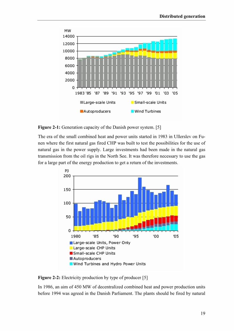
the reluctance of the Danish population, the plans for nuclear power were finally aban-doned in Denmark in 1985. The utilization of wind power for electricity production started back in 1891 at Askov folk high school where Poul la Cour made experiments with a wind turbine producing DC. The experiments included the use of oxyhydrogen gas, produced with electrolysis for light production. When he died in 1908, so did his ideas about wind turbines for large scale electricity production for the time being. During the Second World War, wind power became a renascence with DC wind turbines with a power up to 30 kW from Lykkegård and F.L. Smidt. The next mile stone was the “Gedser Turbine” built by J. Juul in 1957 as a part of a research project. The Turbine was connected to the power system and had an induction generator. This concept was later to be known as the “Dan-ish Concept”. In 1962, it was, however, concluded that wind power production could not compete with the prices of coal and oil at that time. In 1976 the carpenter Christian Riisager built a Danish Concept wind turbine in his back yard and connected it directly to the electrical system of his house. During the tests, the meter started running back-wards. For the electricity company, it was a whole new problematic to consider, and regulations and tariffs for such producers had to be made. But it was also the starting signal of a whole new era of wind power in Denmark. In 1979, the Danish parliament decided that wind turbines approved by the Risø National Laboratory could get 30 % government grant. The vision of the resolution, ENERGI 2000 that came in 1990 was that in 2005, 10 % of the Danish electricity production should come from wind turbines, and private persons were encouraged to invest in wind power projects. To promote the development, the infeed prices were subsidized, and the grid operators were obliged to provide a cheap and unbureaucratic access to the distribution networks. The 10 % target was already reached in the year 2000 [5]. Figure 2-1 shows the development of the in generation capacity in the Danish power system for different types of production units, and Figure 2-2 shows their part in the total electricity production. In 2002, the wind farm, Horns Reef, with a rated power of 160 MW was constructed, and in 2003, the Nysted wind farm with a rated power of 165 MW followed. Since 2003, the total in-stalled capacity of wind power is approximately 3100 MW or 23 % of the total genera-tion capacity. In 2005 wind power covered 18.5 % of the total power production, and in Western Denmark there are periods, where wind power alone can cover the entire load demand.
Distributed generation
19
The era of the small combined heat and power units started in 1983 in Ullerslev on Fu-nen where the first natural gas fired CHP was built to test the possibilities for the use of natural gas in the power supply. Large investments had been made in the natural gas transmission from the oil rigs in the North See. It was therefore necessary to use the gas for a large part of the energy production to get a return of the investments.
In 1986, an aim of 450 MW of decentralized combined heat and power production units before 1994 was agreed in the Danish Parliament. The plants should be fired by natural
Figure 2-1: Generation capacity of the Danish power system. [5]
Figure 2-2: Electricity production by type of producer [5]

Distributed generation
20
gas, bio gas, waste, straw or wood chips. The major advantage of the distributed power plants is that the thermal losses, related to district heating is are smaller when the plant is closer to the consumers, and it is easier to find sites for smaller plants. In 1994, 773 MW of small scale units were installed, and since 2002 the total capacity has been sta-ble around 1500 MW or 12 % of the total capacity.
2.2 Definition Distributed generation is in [6] defined with the following attributes
• Not centrally planned • Not centrally dispatched • Normally smaller than 50 – 100 MW • Usually connected to the distribution systems
A thorough survey of definitions used to classify DG in different countries is presented in [7]. The broader definition, distributed resources, used for example in [8] also in-cludes demand side management. Storage could also be regarded as a distributed re-source.
2.3 DG technologies Below, a list of the typical distributed generator types is given. A more detailed expla-nation is given for example in [6].
• Combined heat and power plants • Wind turbines • Small hydro power units • Photo Voltaic cells • Fuel cells • Micro turbines
In the following, the most common types of wind turbines and CHPs are briefly listed. Presently, the other generation units are practically not used in the Danish system.
2.3.1 Wind turbines Seen from the grid side, the wind turbines that are available on the market today can be divided into the four categories in Figure 2-3 [1]. In the following, at very brief over-view of the concepts is given. A more detailed description can for example be found in [9]. Type A is the fixed speed wind turbine with a directly grid connected squirrel cage in-duction generator. This configuration is often denoted the Danish concept. Often, the rotor speed can be lowered at lower wind speeds by switching to a stator configuration with three rather than two pole pairs. It was the market leading wind turbine type up to 2000, and in the Danish distribution systems it is still the dominant type. The advan-tages are that is cheap and robust. The disadvantages are that the speed cannot be con-

Distributed generation
21
trolled, which means that wind fluctuations generate power fluctuations in the grid, and that it consumes reactive power after a grid fault. The variable slip concept, type B, comprises a wound induction generator with a vari-able rotor resistance. By changing the rotor resistance the characteristic of the torque curve can be modified, and mechanical stress and power fluctuations can be reduced. The stationary slip can be increased up to approximately 10 %, but increasing the slip leads to increased losses in the rotor resistance. Since the emerge of the doubly fed gen-erator, this concept has lost terrain. The doubly fed induction generator, concept C, also comprises a wound induction generator, but here, the electrical power is transferred from the rotor windings to the grid in super synchronous operation through a back-to-back power converter. For sub synchronous operation the power flow is in the opposite direction. The main advantages of this concept compared to the variable slip concept is that a speed range of up to 40 % can be achieved, there are no losses related to an exter-nal rotor resistance and the reactive power can be controlled independently of the active power. The advantage compared to the full scale converter solution is that only a frac-tion of the produced power, proportional to the slip has to go through the converters which means that the power converter typically only has to have a rating of 20 % of the rated power of the wind turbine. A drawback of the concept is that is cannot provide reactive power to the grid during and right after a severe voltage dip.
Finally, concept D with a full scale converter connected to the grid is used for wind tur-bines with synchronous multipole gearless generators and induction squirrel cage induc-
Gearbox
Squirrel cageinductiongenerator
Maincircuitbreaker
CapacitorBank
Mechanically orThyristor switched
TransformerSoftstarter
By-passcontactor
Gridterminal
Contactors
A
Gearbox
Squirrel cageinductiongenerator
Maincircuitbreaker
CapacitorBank
Mechanically orThyristor switched
TransformerSoftstarter
By-passcontactor
Gridterminal
Contactors
A
Gearbox
Woundinductiongenerator
Maincircuitbreaker
CapacitorBank
Mechanically orThyristor switched
TransformerSoftstarter
By-passcontactor
Gridterminal
Contactors
BVariable rotor resistance
Gearbox
Woundinductiongenerator
Maincircuitbreaker
CapacitorBank
Mechanically orThyristor switched
TransformerSoftstarter
By-passcontactor
Gridterminal
Contactors
BVariable rotor resistance
Inductiongenerator Transformer
Gridterminal
Maincircuit
breakers
~~
Gearbox
Rotor sideconverter
Grid sideconverter
C
Inductiongenerator Transformer
Gridterminal
Maincircuit
breakers
~~
Gearbox
Rotor sideconverter
Grid sideconverter
C
Synchronous /inductiongenerator
Transformer
~~Frequencyconverter
Maincircuitbreaker
=~
Rectifier
Gearbox
D
Gridterminal
Synchronous /inductiongenerator
Transformer
~~Frequencyconverter
Maincircuitbreaker
=~
Rectifier
Gearbox
D
Synchronous /inductiongenerator
Transformer
~~Frequencyconverter
Maincircuitbreaker
=~
Rectifier
Gearbox
Synchronous /inductiongenerator
Transformer
~~Frequencyconverter
Maincircuitbreaker
=~
Rectifier
Gearbox
D
Gridterminal
Figure 2-3: Different generator concepts for wind turbines. A: Fixed speed, Danish Concept, B: Variable slip, C: Variable speed doubly fed generator and D: Variable speed full scale converter
Distributed generation
22
tion generators. This concept is gaining in popularity, because the full scale grid con-verter provides a large degree of flexibility which makes it easy to meet different grid code requirements.
2.3.2 Combined heat and power plants Today, a combined heat and power plant has two main functions. Firstly, it must pro-vide heat for a group of consumers or an industrial process, and secondly, it must sell its electrical power for the highest possible price. The hardest constraint is the heat de-mand, because the consumers often rely on heat from only one plant while the electric-ity can be purchased over longer distances. On the other hand, the heat can be stored in heat capacity tanks and to some extend in the heat distribution pipes by raising the tem-perature. In Denmark, a typical distributed CHP has a thermal storage capacity of 6-10 full load hours [10]. There are four main types of combined heat and power plants [6;10].
• Internal combustion reciprocating engines for gas or diesel • Gas turbines • Combined cycle turbines • Steam turbines
Further, there are emerging technologies for very small scale plants like micro turbines and sterling motors.
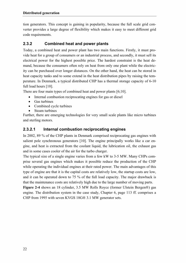
2.3.2.1 Internal combustion reciprocating engines In 2002, 89 % of the CHP plants in Denmark comprised reciprocating gas engines with salient pole synchronous generators [10]. The engine principally works like a car en-gine, and heat is extracted from the coolant liquid, the lubrication oil, the exhaust gas and in some cases cooler of the air for the turbo charger. The typical size of a single engine varies from a few kW to 3-5 MW. Many CHPs com-prise several gas engines which makes it possible reduce the production of the CHP while operating the individual engines at their rated power. The main advantages of this type of engine are that it is the capital costs are relatively low, the startup costs are low, and it can be operated down to 75 % of the full load capacity. The major drawback is that the maintenance costs are relatively high due to the large number of moving parts. Figure 2-4 shows an 18 cylinder, 3.5 MW Rolls Royce (former Ulstein Bergen®) gas engine. The distribution system in the case study, Chapter 6, page 113 ff. comprises a CHP from 1995 with seven KVGS 18G® 3.1 MW generator sets.

Distributed generation
23
2.3.2.2 Gas turbines Gas turbines use the combustion gas to drive a turbine, and the heat is recovered from the exhaust gas which is typically 400 to 600 °C. Because of the high exhaust tempera-ture, the heat can also be used for steam production. The size of a gas turbine varies between 30 kW and 300 MW, but typically, they are not bigger than 15 MW.
2.3.2.3 Combined cycle gas turbine In a combined cycle gas turbine, the exhaust gas of the gas turbine is fed into a heat exchanger which produces steam for a steam turbine. The advantage of this concept compared to the gas turbine is that a larger part of the energy can be converted to elec-trical energy. Typically, the Combined cycle turbines have a size over 20 MW.
2.3.2.4 Steam turbine Combined heat and power plants with steam turbines principally work like traditional thermal power plants with a boiler and one or more steam turbines. In a traditional thermal power plant, the steam is being condensed with cooling water for maximal elec-tricity production. In a CHP, the steam from the turbine is let through a heat exchanger to extract energy for district heating. There are two main types of steam turbines: back pressure and pass-out. In the back pressure turbine, the steam is taken out of the turbine with a high pressure and let through a heat exchanger. With this setup, the ratio between heat and electricity production is fixed. The pass-out turbine also comprises a con-denser. By letting steam through the condenser, the output pressure is lowered which leads to a higher electricity production and a lower heat production. In distributed CHP units, steam turbines are typically driven by waste and solid bio-fuels like straw or wood chips.
Figure 2-4: Rolls Royce KVGS 18G4.2® - 3.5 MW generator-set. With permission from “Rolls-Royce Marine AS, Bergen, Norway”

Distributed generation
24
2.3.2.5 Overview Table 2-1 presents a rough overview of the application of the different CHP types in Denmark. The reciprocating gas engine is the most commonly used generator type, es-pecially for small scale units connected to the 10 kV level and below.
2.4 Technical issues related to grid integration of DG This section gives a brief overview of the issues related to integration of distributed generation and presents relevant literature on each subject. A brief but broad survey of the economical, ecological and technical opportunities and challenges of DG can be found in the paper [11]. Reference [12] provides an overview with focus on the technical issues. More details on the issues are given in the text book [6] which treats most of the subjects mentioned below.
2.4.1 Active power balancing Electricity differs from other energy forms by the fact that it is difficult and expensive to store. In any electrical system, the load and the demand have to be balanced at any time. The balancing it performed differently in different time scales. On the shortest time scale, the power is balanced by the spinning inertia in the system. Large thermal power plants typically have higher inertia constants than small CHPs. Converter fed wind turbines do not have any inertia – seen from the grid side, but they can be programmed to act as virtual inertias as described in [13]. Primary frequency control operates in the time range from a few seconds to 10 minutes. In the Danish grid codes for CHP units over 1.5 MW [14] and wind turbines over 1.5
Internal combus-tion reciprocat-ing engines
Gas turbines Combined cycle turbines
Steam turbines
Efficiency, elec. 30 – 45 % 20 – 42 % 44 – 50 % 20 – 40 %
Efficiency, total 85 – 92 % – 90 % 86 – 88 % 85 – 90 %
Elec./ heat ratio 0.5 - 1.0 0.3 – 0.9 1.0 – 1.3 0.3 – 0.9
Partial load ca-pability
Good Poor Poor Average
Startup costs Low Average High High
Typical size under 3- 5 MW over 30 kW over 20 MW over 10 MW
Relative number in DK, 2002
89 % 6 % 5 %
Relative capac-ity in DK, 2002
45 % 35 % 20 %
Table 2-1: Overview of distributed CHP units in Denmark [10]

Distributed generation
25
MW connected to networks below 100 kV [15] it is already specified that new units must be able to perform primary droop control to the extend that the technology allows this. The principle of performing primary droop control with wind turbines has to the knowledge of the author not been used in the Danish distribution systems at present time, but the concepts have been tested with the Horns Reef offshore wind farm [16]. The longer term balancing is performed by the regulating power market and the spot market [17]. The electricity production from combined heat and power plants can be planned a day ahead and it can be scheduled in periods where the spot price is highest. It can therefore have a stabilizing effect on the spot prices, and does not generate a large demand for regulating power. Wind power, on the other hand, cannot be scheduled and there is always some uncertainty in the forecasts. The impact of wind production on the Nordic system has been described in [18].
2.4.2 Reactive power balance In a distribution system, reactive power is usually not used for active voltage control, but the reactive power capabilities of DG units can be used to balance the reactive power. The problem of reducing the reactive power flow between Danish distribution systems and the transmission systems has been described in [19;20]. Algorithms for optimizing the reactive power compensation have been presented in [21]. The possibility for using DG units with power electronic frequency converters to support the voltage or balance the reactive power in a distribution system is described in [22]. The subject of reactive power balancing is being treated in Section 5.2, page 95 ff.
2.4.3 Voltage profile In distribution systems, the X/R ratio is typically lower than in transmission systems. The consumption of active power always causes a decrease in the bus voltage, which can be compensated with line drop compensation control of the under load tap changers of the transformers. On the other hand, the injection of active power will cause the volt-age in the medium and low voltage networks to increase. The problems related to volt-age rise in distribution systems with DG are discussed in [23-26], and further details are given in Section 5.4.1.1, page 105 ff. The problem of maintaining the voltage in a weak sub transmission system after the connection of a wind farm is discussed in [27].
2.4.4 Power quality Power quality is a measure of how close the voltage at the end user is to being sinusoi-dal with the rated frequency and the rated voltage magnitude. The cut-in and cut-out of units, especially old wind turbines and large capacitors gener-ate transient voltage variations, also known as switching flicker. Fluctuations in the wind speed cause cyclic voltage fluctuations, also denoted continuous flicker. Fre-quency converters can generate harmonic currents.
Distributed generation
26
The inertia and low negative sequence impedance of induction generators and synchro-nous generators can, however also contribute to reduction of voltage fluctuations, har-monic currents and imbalance generated by consumers or other generation units. Definitions and assessment methods for power quality impacts of wind turbines are specified in the standard IEC 61400-21[28]. The theory behind power fluctuations of wind turbines is treated in [29]. Flicker meas-urements of actual wind farms are presented in [30;31].
2.4.5 Protection The protection systems for distribution networks are traditionally constructed for radial systems where the active power flow is always supplied from higher voltage levels to lower voltage levels. As described in [6;32], the connection of production units in the MV and LV leads to the following new challenges.
• Increased fault levels may exceed the capacity of the switch gear. • False tripping of healthy radials with DG units or generators in case of faults in
neighboring radials • Blinding of protection when adjacent DG units feed short circuit current into a
local fault. • Unintended islanding (loss of mains) which can lead to prohibiting of automatic
reclosure of relays, unsynchronized reclosure and in some cases operation of parts of the system without effective grounding.
2.4.6 Stability The main concern when discussing stability of distribution systems with a high penetra-tion of DG is the ability to withstand a fault in the transmission system. The reason is that a single fault in the transmission system will cause voltage dips in several distribu-tion systems which can lead to loss of large amounts of distributed generation or a volt-age collapse. The influence of distributed generation on the transient stability of the transmission sys-tem is discussed in [33]. The short term voltage stability of wind turbines has been as-sessed in [34]. Reference [35] both discusses the stability of wind turbines and small CHP units with synchronous generators. The issue of stability is being further treated in Chapter 5.
2.4.7 Losses One of the advantages which is often mentioned for distributed generation is that it can reduce the system losses by supplying costumers in the vicinity. In systems with a high penetration level of DG and low coincidence between the production and the local load, the DG units can also lead to an increase in system losses. The decrease in losses for integration of photo voltaic generation systems has been assessed for a real system in

Distributed generation
27
[36]. Different methods and relevant references for estimation of the impact of DG on system losses are presented in Chapter 3.
2.4.8 Congestion Like DG can reduce losses when located close to local loads centers, it can also contrib-ute to the reduction of the maximal congestion in the power lines. This means that net-work reinforcements which have become necessary because of growing load demands can be deferred by the installation of local DG units. A method for analyzing the poten-tial deferral of reinforcements when installing different types of DG units is presented in [37].
2.4.9 Control and monitoring The reduced cost and increased reliability of communication and control equipment makes it possible to utilize distributed generation units in a better way. Today, most distribution systems have supervisory control and data acquisition (SCADA) systems to perform control and monitoring from the control room. These systems are proprietary and based on vendor specific standards. To make it possible for products from several vendors to communicate with each other, common communication standards are being developed [38]. The standard, IEC 61850 [39] describes the communication for sub stations, and IEC 61400-25 [40] describes the communication for wind turbines. The utilization of communication systems for distributed control of a large number of DG units has been investigated in [41], and a lot of work is currently going on in this field.


29
3 ACTIVE AND REACTIVE POWER LOSSES
Transmission and distribution of electricity always lead to positive active power losses. According to [42] the losses can be divided into non-technical and technical losses. The non-technical losses represent the consumed energy that the utility companies do not get paid for. Sources of non-technical losses are metering inaccuracies, inaccurate log-ging/reading, meter tampering and illegal connections. The problem with non-technical losses is biggest in developing countries where the metering systems are primitive and theft is widespread due to poverty. The technical losses correspond to the amount of energy that is converted to heat on the way from the producer to the consumer. They can further be divided into load depend-ent losses and load independent losses [42;43]. The load dependent losses can roughly be described as series losses which are given by |I|2·R, where R is the series resistance of cables, overhead lines, transformers etc. Due to the quadratic term, an unbalanced load-ing of a distribution line will lead to higher losses than a balanced load. The load independent losses, also referred to as shunt losses, given by |V|2·G, where G is the shunt conductance, describe the losses in the system which are independent of the loading when disregarding the change in voltage imposed by the change in load. These losses are related to hysteresis and eddy-currents in the iron cores of transformers, and dielectric losses in cables. Further, there are losses related to cooling, operation of switch gear etc. In the power system simulation tool, PowerFactory®, which has been used for the case study in this report, the series and the shunt losses can be summed up separately [44]. In AC systems, the transfer of electricity also leads to reactive power losses [45]. Unlike the active power losses, the inductive reactive power losses can be both positive and negative. Currently, reactive energy is not billed at the end-user like active energy is. The term, non-technical reactive power losses, is therefore not used. Like active power losses, the reactive power losses can be divided into load dependent series losses given by |I|2·X where X is the series reactance, and load independent shunt losses, given by -|V|2·B, where B is the shunt susceptance. Positive reactive series losses are mainly gen-erated by overhead lines and transformers. Negative series losses can be generated by capacitive series compensation. Positive reactive shunt losses are mainly generated by the magnetizing of transformers. Negative reactive shunt losses are generated by ground cables, and shunt capacitors.
Active and reactive power losses
30
The aim of this chapter is to present the general problem of estimating active and reac-tive power losses and allocating them to individual loads and generators in a system with embedded generation.
3.1 Estimation of losses The active and reactive power losses in a system can generally be estimated in two dif-ferent manners. The most straight forward way is to calculate the losses as the differ-ence between the production and the consumption. The advantage of this approach is that is does not require information about the network parameters. The disadvantage is that is requires accurate measurements of all consumers and producers. Since the losses are typically much smaller than the load flows in the system, small inaccuracies in the measurements can lead to large inaccuracies in the loss estimates.
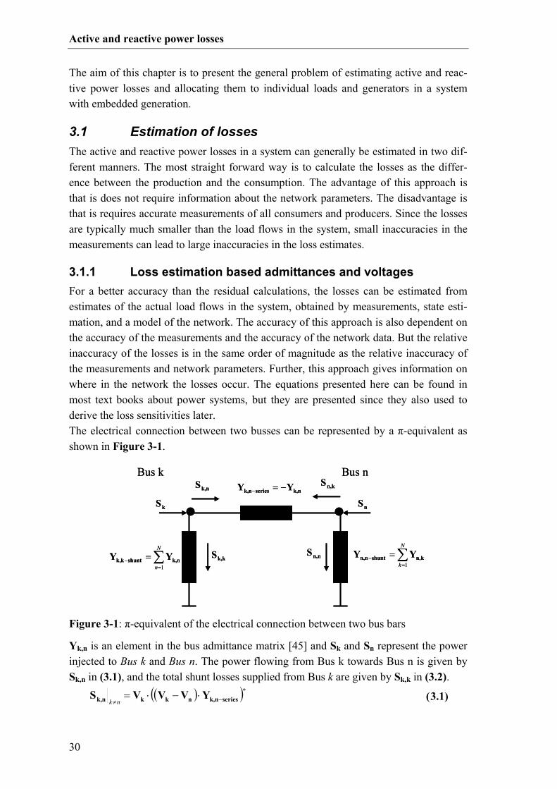
3.1.1 Loss estimation based admittances and voltages For a better accuracy than the residual calculations, the losses can be estimated from estimates of the actual load flows in the system, obtained by measurements, state esti-mation, and a model of the network. The accuracy of this approach is also dependent on the accuracy of the measurements and the accuracy of the network data. But the relative inaccuracy of the losses is in the same order of magnitude as the relative inaccuracy of the measurements and network parameters. Further, this approach gives information on where in the network the losses occur. The equations presented here can be found in most text books about power systems, but they are presented since they also used to derive the loss sensitivities later. The electrical connection between two busses can be represented by a π-equivalent as shown in Figure 3-1.
nk,seriesnk, YY −=−
∑=
− =N
n 1nk,shuntkk, YY ∑
=− =
N
k 1kn,shuntnn, YY
nk,S kn,S
kk,S nn,S
kS nS
Bus k Bus nnk,seriesnk, YY −=−
∑=
− =N
n 1nk,shuntkk, YY ∑
=− =
N
k 1kn,shuntnn, YY
nk,S kn,S
kk,S nn,S
kS nS
Bus k Bus n
Figure 3-1: π-equivalent of the electrical connection between two bus bars
Yk,n is an element in the bus admittance matrix [45] and Sk and Sn represent the power injected to Bus k and Bus n. The power flowing from Bus k towards Bus n is given by Sk,n in (3.1), and the total shunt losses supplied from Bus k are given by Sk,k in (3.2).
( )( )*seriesk,nnkkk,n YVVVS −≠⋅−⋅=
nk ( 3.1)

Active and reactive power losses
31
( )*shuntk,kkkk,k YVVS −⋅⋅= ( 3.2)
The total losses in the series impedances can be derived from the sum of the power in-jections of both ends of each of the connections in (3.1) which yields the expression in (3.3)
( )[ ]∑∑= =
−− ⋅−−+=N
k
N
nnknknk VVVV
1 1
22 )cos(221 *
seriesnk,seriesloss YS δδ ( 3.3)
The shunt losses are given as the sum of (3.2) over all busses.
[ ]∑=
−− ⋅=N
kkV
1
2 *shuntk,kshuntloss YS ( 3.4)
In PowerFactory®, the active and reactive series and shunt losses are automatically summed separately for transformers and lines when performing a load flow calculation. The series losses are referred to as load dependent losses and the shunt losses are re-ferred to as no-load losses. There is, however, a cross coupling, since the loading if the system changes the bus voltages and the shunt elements cause power flows in the lines even when the system is not loaded. It should be noted that the admittances change with changing tap-settings of transformers etc.
3.1.2 Estimation based on current injections and impedances The following method for estimation of network losses is based on the impedance ma-trix and the current injections rather than the admittance matrix and the bus voltages. This formulation is suitable for the loss allocation based on statistical considerations which is presented in Section 3.3. The basic assumption of the method is that the busses in the network can be partitioned in three types: One slack bus, a number of busses without current injections, and a num-ber of busses with current injections. The relation between the bus currents and the bus voltages is given by the bus impedance matrix [45] in (3.5). SLV and SLI are the voltage
and current of the slack bus. IV and II are column vectors with the voltages and cur-rents of the busses with current injections. The busses without sources are not consid-ered.
⋅
=
I
SL
2221
1211
I
SL
I
I
ZZ
ZZ
V
V ( 3.5)
The voltage at the slack bus and the current at the busses with current sources are as-sumed to be known. The current at the slack bus and the voltages at the current busses can be calculated using (3.6) and (3.7) where the matrices, IZ , 12K and 21K are de-
fined in (3.8) to (3.10). The derivation is given in Appendix A page 173.
I12SLSL IKVZI ⋅−= −111 ( 3.6)
SL21III VKIZV +⋅= ( 3.7)

Active and reactive power losses
32
121
11 ZZZZZ 2122I−⋅−= ( 3.8)
12111 ZZK 12
−= ( 3.9)
1−⋅= 112121 ZZK ( 3.10)
The losses can be calculated as the sum of all the power injections into the network (3.11).
IISLSLloss VIVIS ⋅+=H* ( 3.11)
Inserting (3.6) and (3.7) in (3.11) and rearranging and assuming that the impedance ma-trix is symmetrical yields the expression in (3.12).
( ) ( )444 3444 214342144 344 21
effect Crosslosses dependent Loadlosses load-No
**1 2 SL21IIIISL11SLloss VKIIZIVZVS ⋅ℑ⋅⋅++= − HHj ( 3.12)
The expression consists of three terms. The first term describes the no-load losses which are dependent only on the voltage at the slack bus. This includes shunt losses in trans-formers and series losses related to reactive power flows in the shunt elements. The sec-ond term represents the losses which are related to the square of the current infeeds. The last term represents a cross coupling between the two first terms. The term describes the change in losses related to supplying the shunt elements from different busses. For ex-ample, one can think of a transformer with a large magnetizing current which is located far away from the slack point. If a part of the magnetizing current is supplied at a con-nection point close to the transformer, it will contribute to reduction of the overall losses. This effect is not covered by the load dependent quadratic term. If the shunt im-pedances in the system are large compared to the series impedances, it can be seen that
21K will be close to unity and the last term in (3.12) will be relatively small.
In many cases, the active and reactive power injections are known rather than the cur-rent injections which are used in (3.12). The power flows in the system will change both magnitudes and angles of the bus voltages. To take this effect into account, a load flow analysis is required. However, an estimate of the current injections can be achieved us-ing (3.13) and (3.14) where 1 denotes an identity column vector and [ ]/. denotes an element-wise division.
*
*
11SL
IISLIISLI V
SZVIZVV ⋅+⋅≈⋅+⋅= ( 3.13)
[ ]*
*
**
1/.
+⋅≈
SL
IISLII V
SZVSI ( 3.14)
It is believed that the formulation of the total system losses in (3.12) is new. Loss esti-mation and allocation based on current injections have earlier been proposed as the so-called Z-Bus loss allocation method [46]. The major difference between the method proposed in [46] and this method is that the Z-Bus loss allocation method is based on

Active and reactive power losses
33
the full impedance matrix, i.e. no slack bus is assumed. This is an advantage in a large transmission system, where several generators are trading power to balance the system. In the method proposed here, a slack bus is assumed. For a distribution system, this can be justified, since many distribution systems only have one connection point to the transmission system. One advantage of calculating the losses based on the reduced im-pedance matrix is that the diagonal elements, as shown in Section 4.1 page 55, have the physical interpretation of the short circuit impedance at the corresponding bus bar, and the off-diagonal elements are approximately equal to the short circuit impedance in the point of common coupling between the corresponding busses. Also, it makes it possible to separate the load dependent and the load independent losses. A drawback of the formulation with the impedance matrix rather than the admittance matrix is that the sparsity is lower for impedance matrix than for the impedance matrix. This means that for larger systems, the computational requirements are higher for the calculation of losses based on the current injection method than for the methods based on the admittance matrix.
3.1.2.1 Example Figure 3-2 shows an example of a network with a slack bus and two current sources which can both produce and consume active and reactive power.
The relation between the bus currents and the bus voltages is given by the bus imped-ance matrix in (3.15).
⋅
++
+=
=⋅=
C
B
A
DDCDDDDD
DDDDBDDD
DDDDDDAD
C
B
A
III
ZZZZZZZZZZZZ
VVV
IZV ABC ( 3.15)
Calculating the three terms in (3.12) separately gives the expressions in (3.16) to (3.18). (3.16) shows the losses, if the current sources were turned off.
Bus A
Bus B
Bus C
Bus D
ZBD
ZCD
ZAD
ZDD
Figure 3-2: Small example network

Active and reactive power losses
34
( )*
2
DDAD
ASLloss ZZ
VS
+=− ( 3.16)
(3.17) shows the losses, if the voltage on Bus A were set to zero. The diagonal elements represent the losses corresponding to a current going from one of the sources through the parallel connection of ADZ and DDZ . The off diagonal elements represent the cross effect of the two currents.
[ ]
⋅
++
+
+++
⋅=−C
B
DDAD
DDADCD
DDAD
DDAD
DDAD
DDAD
DDAD
DDADBD
CBIloss II
ZZZZZ
ZZZZ
ZZZZ
ZZZZZ
IIS ** ( 3.17)
(3.18) shows the cross coupling between the currents at Bus B and C and the voltage at Bus A. If DDZ is much larger than ADZ or/and ADZ and DDZ have similar X/R ratios this term is very small.
[ ] ADDAD
DD*C
*BCrossloss V
ZZZIIS ⋅
+
ℑ⋅
⋅⋅⋅=−
1
12j ( 3.18)
3.2 Deterministic allocation of system losses Having estimated the time dependent active and reactive power losses in the different components of the system, it can be advantageous to study the cause of the losses. In a liberalized market, this knowledge can be used to avoid cross subsidizing in the trans-mission and distribution fees of consumers and producers [47], to generate incentives of the participants to change the consumption or production in periods with conges-tion[48;49] or to estimate the value of distributed generation in an area [36]. In systems where the investments and operation are partially or fully centrally controlled, the allo-cation of losses can be used to optimize the operation and investments and to minimize the losses. One of the problems about separating the cause of losses is the non linear nature of (3.17). Given a situation where two participants are connected to the same bus and sharing the same line, the series losses can be expressed as in (3.19). V is the volt-age at the common connection point.
( ) ( ) ( )[ ]series*
*212211
series*
*2
*121
seriesloss ZVV
SSSSSSZVV
SSSSS ⋅⋅
ℜ⋅++=⋅
⋅+⋅+
=−
2**
( 3.19)
The two first terms which represent the square of the two current contributions can eas-ily be allocated to the two generators. The last term, however, is a cross term which is dependent on the magnitude of both current contributions and the angle between them. This means that the contribution of one participant on the losses depends on the behav-ior of the neighboring participants. In literature, the following main approaches of loss allocation based on deterministic methods are found [47;50-52]: Pro Rata procedures where the losses are allocated to producers and consumers proportionally to the delivered or consumed energy, Marginal

Active and reactive power losses
35
Loss allocation procedures where the losses are allocated according to the change in losses corresponding to a small change in production or consumption and Proportional Sharing procedures, also referred to as tracing [51], where the losses are allocated ac-cording to the total power flows in the system generated by the participants. Further, the Z-Bus allocation method has been proposed in [46] where the losses are allocated based on the current flows in the system rather than the power flows. The following sections briefly illustrate and compare the marginal loss allocation method to the proportional sharing algorithm.
3.2.1 Marginal loss allocation (Sensitivity analysis) One way of determining the amount of the losses each consumer or producer is respon-sible for is to calculate the marginal change in losses corresponding to a marginal chan-ge in production or consumption[48;52-54].
The marginal loss coefficients (MLC) for transfer of active power, k
loss
PP∂∂ and
k
loss
PQ∂∂
[52;55] represent the change in active and reactive power losses, corresponding to a small change in active power injection in Bus k, provided that the extra injection minus the extra losses is absorbed at the slack bus or several distributed slack busses. Analo-
gously, the MLCs, k
loss
QP∂∂ and
k
loss
QQ∂∂ , can be defined for the transfer of reactive power
[56]. The extra reactive power injection will be absorbed at one or more of the PV-busses or by shunt elements due to change in bus voltages. The MLCs corresponding to active or reactive power transfer of a bus bar are generally positive if there is a surplus of active or reactive power in the vicinity of the bus bar and vice versa. The MLCs can be calculated as described in Appendix A or as described in [55]. Having the MLCs at a given operation point, the total active and reactive system losses can be estimated from (3.20) and (3.21). The factor, κ, is close to 0.5 because of the quadratic shape of the loss curve, but to make sure that the contributions from all pro-ducers and consumers add up to the total load dependent system losses, the factor can be adjusted [52].
loadnoloss
N
k k
lossk
k
losskloss P
QP
QP
PPP −−
=
+
∂∂
+∂∂
= ∑1
κ ( 3.20)
loadnoloss
N
k k
lossk
k
losskloss Q
QP
QPQ −−
=
+
∂∂
+∂∂
= ∑1
κ ( 3.21)
One way of improving the accuracy of the estimated losses is to perform a Taylor ex-pansion of (3.3) and including the second order term. This means that a Hessian matrix with the second order derivatives of the loss with respect to voltage angles and magni-tudes must be calculated. Two different approaches using this approach are presented in [57] and [52].

Active and reactive power losses
36
3.2.2 Proportional sharing of losses (tracing) The principles of flow tracing were originally proposed by Bialek in 1996 in [58]. Methods based on the principles have been proposed by other researchers in several publications, for example [47;59] and [60]. The basic idea of proportional sharing is that the inflows of bus in a network are distrib-uted proportionally between the outflows of the same bus [58]. Figure 3-3 shows an example of a node with three inflows and two outflows. The total power flow out of the node is 100 MW which is the same as the total power flow into the node.
According to the principle of proportional sharing, the 40 MW flowing in Line i,m away from Bus i comprises 40 · 40/100 = 16 MW from Line j,i, 35 · 40/100 = 14 MW from Linek,i and 25 · 40/100 = 10 MW from Linel,i. This flow allocation algorithm is generally referred to as the upstream looking algorithm. Analogously, it can be seen that the 40 MW flowing in Line j-i comprises 60 · 40/100 = 24 MW going towards Line n,i and 40 · 40/100 = 16 MW going towards Bus m. This algorithm is referred to as the down stream looking algorithm. The losses in the individual lines can then be shared among the generators or loads which are responsible for them. The sharing can either be based on the relative power flows or on the square of the power flows. To determine the flows in larger systems, a formalized set of algorithms is needed. In Appendix A, a very brief overview of the algorithms is given. For a more detailed de-scription, refer to [58] or [59].
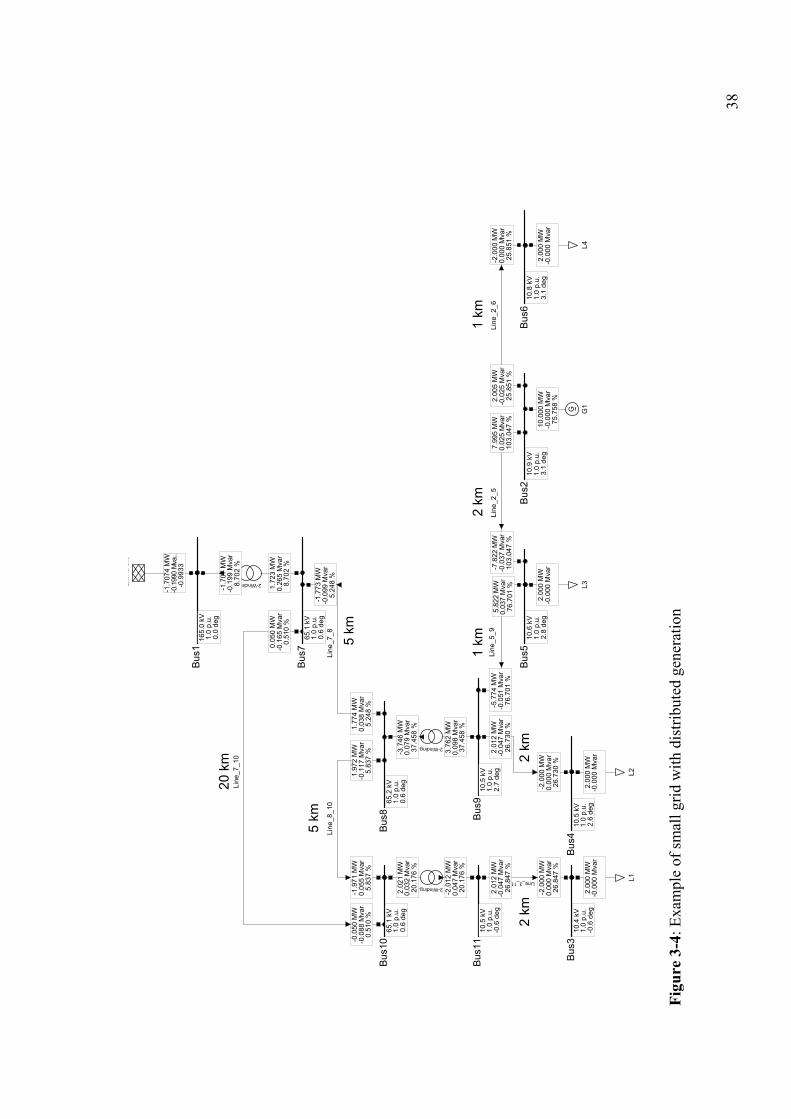
3.2.3 Example Figure 3-4 shows a fictive example of a small distribution system with distributed pro-duction. The result boxes show the solution to a load flow calculation where the con-sumption of each of the loads is 2 MW and the local production is 10 MW. The arrows show the flow direction of the active power. The losses in the transmission system have not been considered in this investigation. The loads and the generators have been mod-
i
j
k
m
n
40
6025
35
40
l
i
j
k
m
n
40
6025
35
40
l
Figure 3-3: The principle of proportional sharing. The numbers indicate power flows in MW

Active and reactive power losses
37
eled as ideal PQ sources. Only one type of lines and transformers has been used on each voltage level. The parameters can be found in Appendix B page 179 ff.
38
2 km
2 km
1 km
2 km
1 km
5 km
5 km
20 k
mLi
ne_7
_10
-0.0
50 M
W-0
.088
Mva
r0.
510
%
0.05
0 M
W-0
.165
Mva
r0.
510
%
L2
2.00
0 M
W-0
.000
Mva
r
Line
_4_9
-2.0
00 M
W0.
000
Mva
r26
.730
%
2.01
2 M
W-0
.047
Mva
r26
.730
%
L4
2.00
0 M
W-0
.000
Mva
r
G ~ G1
10.0
00 M
W-0
.000
Mva
r75
.758
%
Line
_2_6
2.00
5 M
W-0
.025
Mva
r25
.851
%
-2.0
00 M
W0.
000
Mva
r25
.851
%
Line
_2_5
-7.8
22 M
W-0
.037
Mva
r10
3.04
7 %
7.99
5 M
W0.
025
Mva
r10
3.04
7 %
L1
2.00
0 M
W-0
.000
Mva
r
L3
2.00
0 M
W-0
.000
Mva
r
Line
_5_9
-5.7
74 M
W-0
.051
Mva
r76
.701
%
5.82
2 M
W0.
037
Mva
r76
.701
%
Line_3_11
2.01
2 M
W-0
.047
Mva
r26
.847
%
-2.0
00 M
W0.
000
Mva
r26
.847
%
2-Winding..
-3.7
46 M
W0.
079
Mva
r37
.458
%
3.76
2 M
W0.
098
Mva
r37
.458
%
2-Winding..
2.02
1 M
W0.
032
Mva
r20
.176
%
-2.0
12 M
W0.
047
Mva
r20
.176
%
Line
_8_1
0
1.97
2 M
W-0
.117
Mva
r5.
837
%
-1.9
71 M
W0.
055
Mva
r5.
837
%
Line
_7_8
-1.7
73 M
W-0
.099
Mva
r5.
248
%
1.77
4 M
W0.
038
Mva
r5.
248
%
2-Winding..
-1.7
07 M
W-0
.199
Mva
r8.
702
%
1.72
3 M
W0.
265
Mva
r8.
702
%
Ext
erna
l Grid
-1.7
074
MW
-0.1
990
Mva
..-0
.993
3
Bus
410
.5 k
V1.
0 p.
u.2.
6 de
g
Bus
610
.8 k
V1.
0 p.
u.3.
1 de
g
Bus
210
.9 k
V1.
0 p.
u.3.
1 de
g
Bus
310
.4 k
V1.
0 p.
u.-0
.6 d
eg
Bus
1110
.5 k
V1.
0 p.
u.-0
.6 d
eg
Bus
1065
.1 k
V1.
0 p.
u.0.
6 de
g
Bus
510
.6 k
V1.
0 p.
u.2.
8 de
g
Bus
910
.5 k
V1.
0 p.
u.2.
7 de
g
Bus
865
.2 k
V1.
0 p.
u.0.
6 de
g
Bus
765
.1 k
V1.
0 p.
u.0.
6 de
g
Bus
116
5.0
kV1.
0 p.
u.0.
0 de
g
Figu
re 3
-4: E
xam
ple
of sm
all g
rid w
ith d
istri
bute
d ge
nera
tion

39
Figure 3-5 shows the total active and reactive power losses of the system, when the output of the embedded generator is varied between 0 and 10 MW while the load is kept constant. The losses have been split into shunt and series losses. The active power losses reach a minimum when the generator is producing approximately 3.5 MW, and the reac-tive power losses reach the minimum at a production of approximately 6.5 MW. Due to the contribution of the shunt capacitance of the cables, the total reactive power losses are negative, when the local production exceeds 2 MW.
The load dependent active and reactive power losses have been allocated to the loads and the generator according to the principle of marginal loss allocation as described in Section 3.2.1 and proportional load sharing (tracing) as described in Section 3.2.2. Figure 3-6 A and B show the allocation according to the tracing algorithm. The ap-proach has been to calculate the contribution of the generator at Bus2 and loads at Bus 3-6 to the flow in each line element and share half the losses in each line element pro-portionally among the generators contributing to the flows in each line element and the other half among the contributing loads. The slack bus has been included in the set of loads or generators according to the sign of its active power contribution. As seen in Figure 3-6 B, the load with the highest allocated losses at zero production is L4 at Bus 6, since the power has to be supplied all the way from the transmission sys-tem. When the local production exceeds 2 MW, Bus 6 is supplied solely from Bus 2, and the assigned losses correspond to the series losses of Line_2_6. Although the entire power of G1 is flowing in Line_2_6 when the production is below 2 MW, the losses allocated to the other loads are also slightly decreased because the congestion in the remaining network is reduced when L4 is fed locally. The losses allocated to L3 at Bus 5 reach their minimum at a production of approximately 3 MW meaning that the gen-erator is supplying half the load and the rest is supplied from the transmission system. L1 at Bus 3 and L2 at Bus 4 reach their respective minimal losses when they are sup-
Figure 3-5: Total active and reactive power losses in the distribution system when the production from the generator G1 is varied

Active and reactive power losses
40
plied solely from the transmission system but the remaining loads are fed from the gen-erator.
Figure 3-6 C and D show the losses allocated according to (3.20) where κ has been set to 0.5. The losses allocated to the embedded generator are equal to the output multiplied with the derivative of the series losses with respect to the production in Figure 3-5 A. That is why negative losses are allocated to the generator when the production is less than 4 MW. After that point the losses allocated to the generator grow faster with the marginal algorithm than with the tracing algorithm, since the losses allocated to the slack bus are per definition zero and the losses allocated to some of the loads become negative at higher outputs of the generator. The total losses in Figure 3-5 A are in fact reduced when the generation is below 7 MW compared to the situation without distributed generation. The allocation of the series reactive power losses caused by the transfer of active power is shown in Figure 3-7. The big difference between the active and the reactive power losses is that most of the active power losses are generated in distribution lines and es-pecially the low voltage lines while most of the reactive power losses are generated in the transformers and the high voltage lines. Figure 3-7 B shows that the allocated reac-
Figure 3-6: Active power losses allocated to the consumers (B and D) and the produc-ers (A and C) with the tracing method (A and B) and the marginal loss allocation method (C and D)

Active and reactive power losses
41
tive power losses of the loads are much smaller when the loads are supplied locally than when they are supplied through a transformer.
The losses related to the transfer of reactive power can be allocated with the sensitivities in Figure 3-8. Since neither the loads nor the generator exchange any reactive power with the network, only the sensitivities have been plotted. The sensitivities are either negative or zero. This means that injection of a small amount of reactive power would reduce the total system losses. Since there is a surplus of reactive power, when the pro-duction exceeds 2 MW (Figure 3-5 B) the reason for the negative coefficients is proba-bly that an injection of reactive power would increase the voltages and thereby reduce the currents in the system.
Figure 3-7: Reactive power losses allocated to the consumers and the producers with the tracing method (A and B) and the marginal loss allocation method (C and D)

Active and reactive power losses
42
To sum up, the proportional sharing algorithm allocates the losses according to the way the active power is actually flowing in the system. This isn’t necessarily the way the power has been traded. In the example, the losses allocated with the tracing algorithm were split between the consumers and the producers. Another approach would have been to allocate the losses corresponding to a situation without embedded generation to the consumers and allocate the remaining losses to the producers [47]. The losses re-lated to the transfer of reactive power are difficult to separate with the tracing algorithm. One advantage of the proportional sharing algorithm is that the result is not dependent on the definition of a slack bus in the system. This is especially relevant in a very large interconnected transmission system where the power balancing is not performed by one single generator. Also in situations where some local power plants are mainly supplying some local costumers but power is occasionally transferred over longer distances. The marginal loss allocation algorithm allocates the losses according to the influence a change in consumption would have on the losses. Prices based on this allocation method will give the participants an incentive to operate in a way that minimizes the system losses. The fees, however, lead to high costs for larger embedded production units, since the production units have to cover the negative prices of the consumers in the vicinity. One major advantage of the marginal allocation method based on first order sensitivities is that the sensitivity coefficients can be calculated with most commercial power system simulation tools. Because the flow tracing algorithm is assumed to be most suitable for transmission sys-tems and because it is not directly supported by the used power system simulation tool, it is not used further in the case study in Chapter 6.
3.3 Statistical allocation of system losses In the previous sections, it has been shown, how the power losses in a network can be accurately calculated based on the network data and the state of the system.
Figure 3-8: The marginal increase in losses corresponding to a marginal reactive po-wer injection at the different bus bars

Active and reactive power losses
43
In cases where large sets of measurement data is available, statistical methods can be used to separate the causes of the active and reactive power losses from each other and to anticipate future losses based on prognoses. In [19] the causes of the Reactive power exchange between a distribution system and a transmission system have been allocated to the wind turbines, CHPs and consumers using a linear regression analysis. This ap-proach has also been used in [61] to determine the impact of wind turbines on the reac-tive power losses in the distribution transformers of a system. [62;63] propose a cluster wise linear regression method based on fuzzy logic to anticipate and allocate active power losses in a distribution system.
3.3.1 Regression analysis The idea of the linear regression analysis is to represent the losses as a linear combina-tion of a number of input variables. Generally, the linear regression problem can be spe-cified as (3.22) [64]. y is a column vector with one sample of the estimated quantity per
entry, X is a matrix with a row for each observation and a column for each input pa-
rameter, B is a column vector with one coefficient per input parameter, and1 is an identity column vector with the same size as y .
BXxbxbxbby k22110 ⋅=++++= k...1ˆ ( 3.22)
There are standard algorithms for determining the coefficient vector which leads to the smallest quadratic deviation between the measured and the estimated output. However, it is important to know the basic structure of the problem to select a set of input parame-ters which provide sufficient but not redundant information. The basis for the statistical model is (3.12), page 32. Assuming that the voltage at the slack bus remains relatively constant, (3.23) can be assumed to be constant. It is there-fore expected that b0 in (3.22) when used to estimate the complex losses of the system will be close to (3.23).
( ) **1SL11SLshuntloss VZVS −
− = ( 3.23)
The load dependent losses in (3.24) depend on the complex current injections of the producers and consumers.
IZIS Iseriesloss
H=− ( 3.24)
To get (3.24) on a form which is compatible with (3.22), the impedance matrix must be isolated. (3.24) is reformulated as (3.25) where N is the number of busses with current injection.
[ ] [ ] [ ]∑∑= =
− =N
j
N
ijiji
1 1,
*Iseriesloss ZIIS ( 3.25)
If the system does not contain phase shifting transformers, the impedance matrix will be symmetrical [45]. This means that the cross terms in (3.25) should only be included once, as shown in (3.26).

Active and reactive power losses
44
[ ] [ ] [ ] [ ] [ ] [ ] [ ] [ ] [ ] [ ]( ) [ ] jijijiijijjiji ,
***
,
*
,
*III ZIIIIZIIZII
+=+ ( 3.26)
To get an exact match between the regression model and the system, the last term in (3.12) should also be included. This means that input parameters corresponding to the product of the current and the voltage at the slack point should be added to the input vector (3.27).
[ ] ( ) SL21crossloss VKIS ⋅ℑ•⋅⋅=− .2*
j ( 3.27)
Including all the previously mentioned terms as input parameters for the regression ana-lysis leads to the expression in (3.28). The size of B is 1 + 0.5 · N · (N-1) +2 · N. If there are no tap changing transformers and switchable capacitor batteries in the sys-tem, the model in (3.28) gives a complete description of the losses. This means that if
lossS and X are exactly known, for a large number of samples, and the input variables
are not linearly dependent or constant, a regression analysis will give the B -vector in (3.28).
[ ] [ ][ ] [ ] [ ] [ ]
[ ] [ ][ ]
[ ]
( )[ ][ ]
[ ][ ]( )
[ ]( )
ℑ
ℑ
⋅
⋅
⋅
+
⋅
=⋅=
−
1,
1,1
,
2,1
1,1
*1
*
*1
*
1*22
*1
1*1
*
2
2
ˆ
N
NN
T
N
NN
j
j
21
21
I
I
I
11
SL
SL
SLSL
loss
K
K
Z
Z
Z
Z
VI
VI
II
IIII
II
VV
BXS
M
M
M
M ( 3.28)
If the current infeeds are not known, they can be estimated using (3.14), page 32, or by assuming that the voltage has a magnitude of 1 p.u. and an angle of 0 in the entire sys-tem which is equivalent to inserting the conjugate of the complex power contributions. One problem with the regression analysis is that many of the current injections are high-ly correlated with each other. For example wind farms which are located close to each other. This problem is denoted multicollinearity and can lead to a large variance in the estimated coefficients when analyzing different samples. The problem of multicollinear-ity can partly be overcome by applying a Ridge Regression or a Principal Component Regression, which can reduce the variance of the estimated coefficients at the cost of a bias in the estimated output vector [65-67].
3.3.1.1 Aggregation of current sources In a real distribution system, there is usually a very large number of consumers and pro-duction units. In the BOE case Chapter 6, there are for example 721 aggregated loads,

Active and reactive power losses
45
65 induction machines and 29 synchronous machines in the model. With 815 current sources, (3.28) would require 333336 elements in the input vector, which would not be realistic. Further, there are not measurements of each of the 400 V loads in the system. Therefore, it is advantageous to group some of the sources together and assume that they behave as one lumped source, connected to one virtual node. The grouping of simi-lar components also reduces the problem of multicollinearity. Assuming that the current injections can be expressed as a linear combination of a re-duced number of aggregated currents like in (3.29), the load dependent losses can be calculated exactly using (3.30) and (3.31).
redII IKI ⋅= ( 3.29)
redIIIredseriesloss IKZKIS ⋅⋅⋅⋅=−HH
( 3.30)
( ) SL21Iredcrossloss VKKIS ⋅ℑ⋅⋅⋅=−HH
j 2 ( 3.31)
When the reduced current vector is inserted in (3.28), the estimated B -vector will con-tain elements from III KZK ⋅⋅H and ( )21I KK ℑH .
IK is a transformation matrix with a number of rows corresponding to the number of
busses in the system and a number of columns corresponding to the number of aggre-gated currents. One approach is to define an aggregated current for each feeder based on the sum of all loads of the feeder and another aggregated current based on the sum of all production units of the feeder. Often, only the total power of the loads of a feeder is known. To estimate an aggregated current for the feeder, an aggregated voltage must be assumed. As a first approach, the voltages at the connection points of the feeders can be used as basis for calculating the current at the virtual nodes. The method of loss allocation based on aggregated loads and consumers has been used in the investigation of the losses in the BOE network, presented in [68].
3.3.2 Covariance analysis The reduced impedance matrix, IZ , shows how the different cross products of the cur-
rents affect the losses. The contribution of the cross products to the mean losses is de-pendent on the simultaneity between activity of the different producers and consumers. A measure of the simultaneity is given by the covariance matrix. The covariance matrix of a random vector is defined as (3.32), where E denotes the expected values [66]. The generalization of the theory to include complex random vectors is discussed in [69].
[ ] [ ]( ) [ ]( )[ ]HFFFFF EEEcov −⋅−= ( 3.32)
Rearranging (3.32), the expected value of the outer product of the vector with it self can be expressed as (3.33).
[ ] [ ] [ ] [ ]HHFFFFF EEcovE ⋅+=⋅ ( 3.33)

Active and reactive power losses
46
To use (3.33) to estimate the mean value of the losses in a system based on the mean values and the covariance of the current infeeds, (3.25) is reformulated as (3.34), where [ ]•. denotes an element-wise multiplication, and 1 is a column vector with a number of
ones corresponding to the number of current busses. I is a column vector of complex current injections at the different bus bars. Every current is assumed to be a stochastic variable with a mean value and a variance.
( )[ ][ ] ( ) [ ] 1.11.1**
⋅
•⋅⋅=⋅•⋅=− IIseriesloss ZIIZIIS
HTTT ( 3.34)
Inserting the expected value of the conjugate of the outer product of the current vector with it self, (3.35), in (3.34) yields (3.36)
( ) [ ] [ ] [ ]( )**EEcovE
HHIIIII ⋅+=
⋅ ( 3.35)
[ ] [ ] [ ] [ ] [ ] 1.EEcov1E*
flowsmean from Contr. variancefrom Contr.
⋅
•
⋅+⋅=− Iseriesloss ZIIIS 43421321
HT ( 3.36)
Equation (3.36) shows that the effect of the mean values of the current infeeds on the losses can be separated from the effect of the covariance between the current infeeds on the losses. The cross term of (3.31) could be considered a part of the losses related to the mean power flows. Because if the voltage at the slack point is relatively constant, this term depends on the mean currents. Before multiplying with the identity vectors, the expected losses will form an N by N matrix. The real part of the diagonal elements will always be positive. This means that any traffic of active and reactive current in the system will cause active power losses. The off-diagonal elements can either be positive or negative, dependent on the loading of the network. The real part of the term containing the mean values is difficult to change. The mean value of the production or consumption over longer period is given by the actual utilization of the energy. The mean value of the reactive power can be changed, e.g. by installing or removing a capacitor or changing the power factor of a synchronous machine. The diagonal elements of the covariance matrix describe the variation of the consumption of each consumer. The off-diagonal elements describe the simultaneity of the variations of different current sources. Traditionally the information contained in the covariance matrix has been represented with a coincidence factor or Velander’s coefficients [43]. The simultaneity between different loads and productions is caused by several effects with different time periods including hourly, daily, weekly and seasonal variations. An estimate of the mean values and covariances therefore only describes the behavior within the period where the measurements were taken. The element wise product of the covariance matrix and the reduced impedance matrix can give an indication of where there is potential for power savings, e.g. by changing the production pattern of a CHP to better match the load pattern of a group of consum-ers in the vicinity. The impedance matrix may not be constant during the entire period

Active and reactive power losses
47
of consideration. For example, the under load tap changers of the transformers change all the time. If the changes are relatively small, a mean value of the impedance matrix can be used. Alternatively, analysis can be performed separately for time periods with different network configurations. If the reduced impedance matrix is not known for the system, it can be estimated with a linear regression as described earlier.
3.3.3 The influence from reactive power flows The current dependent losses can be split into contributions from the active power trans-fer, the reactive power transfer and a cross effect between the two. Equation (3.37) shows the separation of the current injections into a part corresponding to the real power injections and a part corresponding to the reactive power injections. The changes in voltage caused by the current injections have not been considered.
[ ]( ) [ ]( ) [ ]( )***/././. VQVPVSIII QP j+==+= ( 3.37)
[ ]( ) [ ]( )**/. and /. VQIVPI QP j== ( 3.38)
Inserting (3.37) in (3.34) yields (3.39)
( ) [ ] 1.1*
effect CrossQ from Contr,P from Contr.
⋅
•
⋅+⋅+⋅+⋅⋅=− IQPPQQQPPseriesloss ZIIIIIIIIS 444 3444 214342143421
HHHHT ( 3.39)
The three terms in (3.39) represent the contribution from the active power injections, the reactive power injections and the cross effect. Since the transfer of active power is usu-ally regarded as the main objective, the cross effect could be considered a part of the losses, allocated to the reactive power.
3.3.4 Example To illustrate the application of the statistical methods, the example in Section 3.2.3 is revisited. Where the sensitivity analysis and the proportional sharing algorithm focused on a single operation point, the statistical methods presented here focus on the analysis of a large set of operation points. As basis for the analysis, time profiles are generated for the active and reactive power production and consumption of G1, L1, L2, L3 and L4. The data is generated based on mean values of different feeders in the BOE case, but each of the load characteristics have been scaled so that they have the same vari-ance, mean value and average power factor. Figure 3-9 shows the time dependent ac-tive power profiles for one week with a resolution of 15 min, and Figure 3-10 shows the time dependent reactive power profiles. The voltage at the slack bus is kept constant at 1 p.u.

Active and reactive power losses
48
Estimates of the covariance between the current infeeds is shown in Table 3-1. They have been calculated using the function cov() in Matlab® with a normalization of N
Figure 3-9: Active power production and load profile of the example
Figure 3-10: Reactive power production and load profile of the example
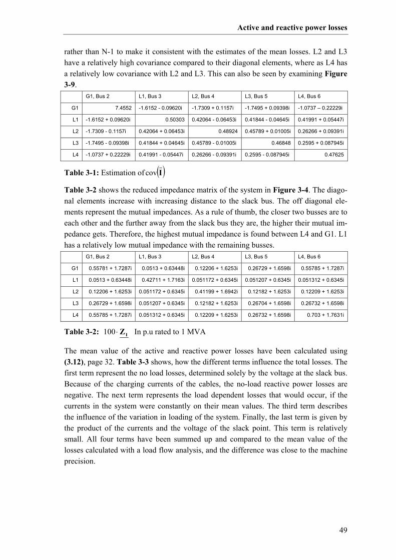
Active and reactive power losses
49
rather than N-1 to make it consistent with the estimates of the mean losses. L2 and L3 have a relatively high covariance compared to their diagonal elements, where as L4 has a relatively low covariance with L2 and L3. This can also be seen by examining Figure 3-9.
Table 3-2 shows the reduced impedance matrix of the system in Figure 3-4. The diago-nal elements increase with increasing distance to the slack bus. The off diagonal ele-ments represent the mutual impedances. As a rule of thumb, the closer two busses are to each other and the further away from the slack bus they are, the higher their mutual im-pedance gets. Therefore, the highest mutual impedance is found between L4 and G1. L1 has a relatively low mutual impedance with the remaining busses.
The mean value of the active and reactive power losses have been calculated using (3.12), page 32. Table 3-3 shows, how the different terms influence the total losses. The first term represent the no load losses, determined solely by the voltage at the slack bus. Because of the charging currents of the cables, the no-load reactive power losses are negative. The next term represents the load dependent losses that would occur, if the currents in the system were constantly on their mean values. The third term describes the influence of the variation in loading of the system. Finally, the last term is given by the product of the currents and the voltage of the slack point. This term is relatively small. All four terms have been summed up and compared to the mean value of the losses calculated with a load flow analysis, and the difference was close to the machine precision.
G1, Bus 2 L1, Bus 3 L2, Bus 4 L3, Bus 5 L4, Bus 6
G1 7.4552 -1.6152 - 0.09620i -1.7309 + 0.1157i -1.7495 + 0.09398i -1.0737 – 0.22229i
L1 -1.6152 + 0.09620i 0.50303 0.42064 - 0.06453i 0.41844 - 0.04645i 0.41991 + 0.05447i
L2 -1.7309 - 0.1157i 0.42064 + 0.06453i 0.48924 0.45789 + 0.01005i 0.26266 + 0.09391i
L3 -1.7495 - 0.09398i 0.41844 + 0.04645i 0.45789 - 0.01005i 0.46848 0.2595 + 0.087945i
L4 -1.0737 + 0.22229i 0.41991 - 0.05447i 0.26266 - 0.09391i 0.2595 - 0.087945i 0.47625
Table 3-1: Estimation of ( )Icov
G1, Bus 2 L1, Bus 3 L2, Bus 4 L3, Bus 5 L4, Bus 6
G1 0.55781 + 1.7287i 0.0513 + 0.63448i 0.12206 + 1.6253i 0.26729 + 1.6598i 0.55785 + 1.7287i
L1 0.0513 + 0.63448i 0.42711 + 1.7163i 0.051172 + 0.6345i 0.051207 + 0.6345i 0.051312 + 0.6345i
L2 0.12206 + 1.6253i 0.051172 + 0.6345i 0.41199 + 1.6942i 0.12182 + 1.6253i 0.12209 + 1.6253i
L3 0.26729 + 1.6598i 0.051207 + 0.6345i 0.12182 + 1.6253i 0.26704 + 1.6598i 0.26732 + 1.6598i
L4 0.55785 + 1.7287i 0.051312 + 0.6345i 0.12209 + 1.6253i 0.26732 + 1.6598i 0.703 + 1.7631i
Table 3-2: IZ⋅100 In p.u rated to 1 MVA

Active and reactive power losses
50
The contribution of each of the elements in column two of Table 3-3 is shown in Table 3-4. The matrix has been made symmetrical by averaging the upper and the lower trian-gle matrix so that the sum of all elements in a column is equal to the sum of all elements in the corresponding row. The sum of each column, Sum1, gives an indication of the contribution of each current source to the losses. The cross effect between two sources is shared equally between them. Sum2 is the sum of each column and the corresponding row. This can be interpreted as the decrease in system losses, if the source under con-sideration were turned off, and the output of all other sources remained constant.
Table 3-5 shows the effect of the covariances of the components. Sum1 and Sum2 have the same meaning as in Table 3-4. The diagonal elements are all positive because any variation will increase the losses compared to a constant operation. The off diagonal elements in row 1 and column 1 are negative, since the correlation between the produc-tion unit and the loads contribute to reduction of the losses. However, the diagonal ele-ment corresponding to G1 is larger than the sum of its off diagonal elements. This means that the total losses would be reduced by 14.3 kW, if G1 would run constantly on its mean value. Since the mean value of generation caused a saving of 84.7 kW com-pared to the situation without G1, the total savings due to the presence of G1 are 70.3 kW.
( )*12 −11SL ZV
No –load losses
[ ] [ ]( ) [ ] IZII •.EE*H
Mean value dep. losses
[ ]( ) [ ] IZI •.cov*
Variance dep. losses
[ ] ( ) SL21I VKI 2 ℑ⋅H
EjCross effect
Sum
28.265 - 452.73i 70.479 + 387.21i 27.61 + 38.081i -2.4689 + 5.4168i 123.84 - 22.079i
Table 3-3: The influence of the different terms in (3.12) on the mean losses. All the numbers are in kVA
G1, Bus 2 L1, Bus 3 L2, Bus 4 L3, Bus 5 L4, Bus 6
G1 56.549 + 175.25i -3.637 - 44.982i -8.6671 - 115.41i -18.857 – 117.09i -39.439 – 122.22i
L1 -3.637 - 44.982i 21.189 + 85.145i 2.5422 + 31.519i 2.5274 + 31.316i 2.5379 + 31.381i
L2 -8.6671 - 115.41i 2.5422 + 31.519i 20.497 + 84.288i 6.0215 + 80.337i 6.0474 + 80.506i
L3 -18.857 - 117.09i 2.5274 + 31.316i 6.0215 + 80.337i 13.114 + 81.51i 13.156 + 81.681i
L4 -39.439 - 122.22i 2.5379 + 31.381i 6.0474 + 80.506i 13.156 + 81.681i 34.669 + 86.95i
Sum1 -14.052 - 224.46i 25.159 + 134.38i 26.441 + 161.24i 15.962 + 157.75i 16.97 + 158.3i
Sum2 -84.653 - 624.16i 29.129 + 183.61i 32.385 + 238.19i 18.809 + 233.99i -0.72851 + 229.65i
Table 3-4: Estimate of the contribution from the mean power flows
[ ] [ ]( ) [ ] ][ 1000.EE*
kVAH ⋅• IZII . The matrix has been made symmetrical for read-
ability. Sum1 is the sum of each column, and Sum2 is the sum of each column and its corresponding row.

Active and reactive power losses
51
It would be possible to minimize the losses in the system while keeping the mean pro-duction and consumption by choosing the covariance matrix that minimizes the sum of Table 3-5. Obviously, the optimal solution would be a covariance matrix with all zeros corresponding to a constant production and consumption, but if the load profiles are given, an optimal production pattern can be generated. It should, however, be noted that some CHPs run at the highest efficiency, if the generators are running at full load. Further, the costs of the losses are small compared to the variations in electricity prices.
3.4 Summary Different methods have been presented for calculation and allocation of active and reac-tive power losses in a power system, and the methods have been illustrated with some simple examples. The two existing algorithms for loss allocation, proportional sharing (flow tracing) and marginal loss allocation have been compared. The major difference between the two algorithms is that the marginal loss allocation algorithm assumes the existence of a slack bus in the system, which is not the case for the proportional sharing algorithm. It is concluded that the proportional sharing algo-rithm is mostly suited for larger interconnected transmission systems, while the mar-ginal loss allocation algorithm can be used for distribution systems where the connec-tion to the transmission system constitutes a suitable choice of slack point. The main advantages of the marginal loss allocation algorithm is that the pricing gives the partici-pants incentives to adjust their consumption/production towards a situation with mini-mal losses. Another advantage is that the calculation of marginal losses is a feature that is available in most power system simulation tools. A new method for loss allocation based on current injections and the short circuit im-pedances has been presented. The method makes it possible to identify the cross effects between different participants. The method can also separate the losses into a part which
G1, Bus 2 L1, Bus 3 L2, Bus 4 L3, Bus 5 L4, Bus 6
G1 41.586 + 128.88i -0.8286 - 10.248i -2.1127 - 28.133i -4.6764 – 29.039i -5.9894 - 18.56i
L1 -0.8286 - 10.248i 2.1485 + 8.6335i 0.21525 + 2.6688i 0.21427 + 2.6549i 0.21546 + 2.6642i
L2 -2.1127 - 28.133i 0.21525 + 2.6688i 2.0156 + 8.2886i 0.55781 + 7.4421i 0.32069 + 4.2692i
L3 -4.6764 - 29.039i 0.21427 + 2.6549i 0.55781 + 7.4421i 1.2511 + 7.7757i 0.69371 + 4.3071i
L4 -5.9894 - 18.56i 0.21546 + 2.6642i 0.32069 + 4.2692i 0.69371 + 4.3071i 3.3481 + 8.397i
Sum1 27.979 + 42.897i 1.9649 + 6.3732i 0.9966 - 5.4644i -1.9596 - 6.8588i -1.4114 + 1.0774i
Sum2 14.372 - 43.083i 1.7812 + 4.113i -0.02241 - 19.217i -5.1702 - 21.493i -6.171 - 6.2423i
Table 3-5: Estimation of the contribution of the variance of the power flows.
[ ]( ) [ ][ ] ][ 1000.cov*
kVA⋅• IZI The matrix has been made symmetrical for readability.
Sum1 is the sum of each column, and Sum2 is the sum of each column and its cor-responding row.

Active and reactive power losses
52
is dependent on the mean production / consumption and a part which is dependent on the covariance, i.e. between different loads productions. The losses imposed by the co-variance of the flows represent the maximal potential saving which can be achieved by changing the production/consumption time patterns while maintaining the mean flows. Like the marginal loss allocation, this method requires the definition of a slack bus, which is not considered a problem in a distribution system. The current injection method has also been used to formulate a linear regression prob-lem for allocation of losses in a mathematically strict way. Although it is often more convenient to use active and reactive power injections rather than currents, the analysis has demonstrated which approximations this approach depends on.

53
4 STABILITY OF DISTRIBUTION NETWORKS WITH DG
In an AC power system, it is mandatory that the frequency and the voltage magnitudes are kept close to the nominal values at all times. Traditionally, the frequency and volt-age control has been managed by large central thermal or hydro power plants. In the Western Danish system, for example, the TSO, Energinet.dk, pays a fixed amount per year to have at least three spinning plants and one stand by plant connected to the 150 kV network to ensure stability of the system [70]. Many of the text books dealing with power system stability, for example [71], focus on the stability in transmission systems fed solely by synchronous generators with various prime movers. Power system stabil-ity problems are typically classified according to three criteria. Firstly, distinguishing between angle and voltage stability is made. Angle stability is caused by lack of syn-chronizing torque between synchronous generators and voltage stability is caused by lack of reactive power in areas with high load demand. Secondly, stability problems are divided into short term and long term effects. Finally, in non-linear systems, there are generally three different ways, instability can occur: lack of a stable equilibrium, lack of attraction to a stable equilibrium and lack of damping. The classification and assessment of power system stability are thoroughly described in many text books and papers, for example [71-74]. During the nineties a great number of Danish concept wind turbines with squirrel cage induction generators (SCIG) connected directly to the grid were installed in the Danish system. To avoid unintentional islanding and large reactive power deficits after a grid fault, these wind turbines were ordered to disconnect at abnormal grid conditions [75]. As the penetration of wind turbines has increased, the wind power production will in some periods constitute a considerable part of the total production in the area. If a large part of the wind turbines disconnect after a short circuit in the transmission system, the load demand which was covered by the wind turbines before the fault, must be imported or covered by increased productions of thermal power plants. Therefore, the Danish TSO along with many other TSOs has issued a grid code for wind turbines which re-quires the wind turbines to stay connected after a three phase short circuit in the trans-mission system [15;76-80]. If a large number of wind turbines with SCIGs stay con-nected during and after a grid fault, there is a risk of short term voltage stability prob-lems due to the reactive power consumption of the generators. This problem is by some
Stability of distribution networks with DG
54
denoted “Speed stability”, since it has to do with over speeding of the induction genera-tors [81]. Vladislav Akhmatov has made a large contribution to the understanding of this and other problems related to stability of power systems with a large penetration of wind power [34;82-85]. The work includes the modeling of the wind turbines, aggrega-tion of wind farms and simulation of larger systems with wind power. The ability of a wind turbine to stay connected during and after a large grid disturbance is often referred to as “Fault Ride Through Capability” (FRT). For constant speed active stall wind turbines with SCIGs, the transient stability can be improved by pitching the blades and thereby reducing the output power when a fault is detected [84]. For variable speed wind turbines with doubly fed induction generators, the major problem is that a short circuit causes large current transients in the rotor cir-cuit. The solution to that problem is to deactivate the rotor converter and short circuit the rotor windings with an external resistance. This technique is also referred to as “Crow Bar Operation” [86]. For a wind turbine with full scale converter, the challenge is to maintain a stable DC link voltage during and after the fault and to avoid tripping of the converter due to over current in the semiconductors. This problem is mainly related to choosing the right control scheme. As described in [87] which is written by represen-tatives of the Danish, German, Spanish and Irish TSOs, it is still unclear how the rules regarding behavior of the wind turbines connected to distribution systems should be enforced to ensure proper operation of the local protection equipment in the distribution systems. Combined heat and power plants also constitute a potential risk of losing power produc-tion after a short circuit. To avoid unintentional islanding and asynchronous reconnec-tion, many smaller CHPs are equipped with synchronous under-voltage relays which disconnect the units if the positive sequence of the voltage gets below a certain thresh-old. This can lead to loss of a large number of units in case of a fault in the transmission system [88]. Accurate simulations of power systems including different kinds of wind turbine gen-erators can today be performed with standard commercial power system simulation tools. For example, [89] describes a comparison between the four different simulation tools, PSCAD®, SIMPOW®, PSS/E® and PowerFactory® for simulation of short term stability of a wind turbine after symmetrical and unsymmetrical grid faults. A detailed simulation can point out some problems in a specific system, but in order to choose the optimal solution, it is important to know the nature of the problem. More theoretical approaches based on the use of Lyapunov energy functions for explicit evaluation of short term voltage stability of systems with induction generators have been proposed in [35]. The methods have, however, only been demonstrated for a system with a single induction generator with a lumped rotor connected to an infinite bus bar. But in the fu-ture such algorithms may be incorporated in power system simulation tools.
Stability of distribution networks with DG
55
The objective of this chapter is to qualitatively describe the influence of the network topology on the network parameters and the influence of the different network parame-ters on the stability of a distribution network with DG.
4.1 Thevenin equivalent and short circuit power It has been shown for example in [90] that the speed stability of a wind turbine or a wind farm with SCIGs can be roughly assessed by analyzing quasi stationary torque curves of an aggregated generator connected to a Thevenin equivalent network. In this section, this theory will be used to evaluate the effect of wind farms connected in differ-ent places in the distribution network. The basic theory behind network reduction and calculation of Thevenin equivalents is textbook material. A very thorough and systematic description of the topological back-ground can be found for example in [45;91]. The idea behind the Thevenin representation of a network is to regard all generators, compensation units and loads as voltage sources, current sources, or impedances. Due to the nonlinear behavior of the components, the linearization is only valid for small devia-tions from a stationary point or large deviations with a short duration. This is also the approach which is used for stationary calculation of short circuit currents in most power system simulation tools. PowerFactory® offers two different ways of calculating short circuit currents based on steady state analyzes. The most accurate method which is referred to as the “Complete Method” is based on a superposition algorithm. The approach is to firstly to perform a pre fault load flow calculation to determine tap settings, bus voltages, branch currents etc. Secondly, a linear calculation is performed where all voltage sources are short cir-cuited and the pre fault voltage, shifted 180 degrees, is inserted at the short circuit point behind the short circuit impedance. The short circuit currents in the system can then be found as the sum of the currents of the two calculations. Once the non-linear load flow problem has been solved for a given pre fault situation, short circuit calculations can be performed at a number of bus bars in the system using only fast linear calculations. A synchronous machine can be represented as a constant voltage behind the subtransient reactance for determination of the fault currents during the first few AC periods or a constant voltage behind the transient reactance for calculation of the fault currents in the time range of the transient time constant. A voltage source converter like a STATCOM can be represented either as a voltage source behind its filter reactance or a constant current source, where the voltage or the current is equal to the pre-fault value. An SVC is represented as the pre fault susceptance [44]. Alternatively, the short circuit currents can be calculated according to the IEC 909 or the ANSI C37 standards. These methods do not consider loads, current sources and shunt capacitors.

Stability of distribution networks with DG
56
In a running system, the short circuit power for a given situation can be estimated from online measurements of naturally occurring events in the system [92] or by imposing a test signal for example with a power converter [93]. With a few modifications, the Thevenin equivalent circuit seen from a given bus under consideration can be calculated analogously to (3.5) to (3.10) page 31 ff. In (3.5) it is assumed that the system only has one voltage source, namely the slack bus. When dealing with short term effects related to short circuits, the flux linkage of genera-tors also constitute voltage sources which can be considered constant over a short pe-riod. Therefore, the slack bus must be substituted with a vector of constant voltage bus-ses as expressed in (4.1). In a typical distribution system with an infeed from a trans-mission system, a virtual slack bus behind the short circuit impedance at the connection point of the distribution system can be inserted as one of the constant voltage nodes. The node, where the Thevenin equivalent circuit is to be calculated must be included in the set of constant current nodes.
⋅
=
I
V
I
V
I
I
ZZ
ZZ
V
V
2221
1211 ( 4.1)
The voltages in the constant current busses are then given by (4.2), where IZ and
21K are defined in (3.8) and (3.10) page 32 ff.
V21III VKIZV +⋅= ( 4.2)
The Thevenin impedance at bus number n in the set of fixed current busses is then given by the nth diagonal element of the reduced impedance matrix (4.3).
[ ]nn,InTh ZZ =− ( 4.3)
The Thevenin voltage at the nth bus is calculated by setting the current of the bus under consideration to 0 in (4.2) and maintaining all other voltages and currents (4.4).
[ ][ ] 0=− =
nn
IIInTh VV ( 4.4)
Both magnitude and angle relative to a common reference frame of the current and volt-age sources must be known. These can be found using a standard load flow algorithm. Defining the short circuit power, SSC, as the product of the fault current and the nominal voltage yields the expression in (4.5) where * denotes the complex conjugate.
*Th
ThSC Z
VS nominalV
= ( 4.5)
4.2 Danish Concept wind turbines This section briefly describes some of the problems related to Danish Concept wind turbines.
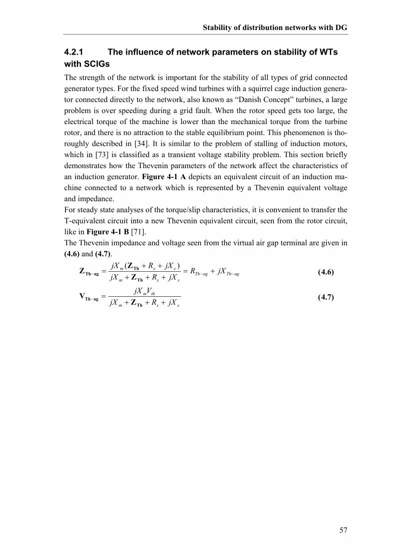
Stability of distribution networks with DG
57
4.2.1 The influence of network parameters on stability of WTs with SCIGs The strength of the network is important for the stability of all types of grid connected generator types. For the fixed speed wind turbines with a squirrel cage induction genera-tor connected directly to the network, also known as “Danish Concept” turbines, a large problem is over speeding during a grid fault. When the rotor speed gets too large, the electrical torque of the machine is lower than the mechanical torque from the turbine rotor, and there is no attraction to the stable equilibrium point. This phenomenon is tho-roughly described in [34]. It is similar to the problem of stalling of induction motors, which in [73] is classified as a transient voltage stability problem. This section briefly demonstrates how the Thevenin parameters of the network affect the characteristics of an induction generator. Figure 4-1 A depicts an equivalent circuit of an induction ma-chine connected to a network which is represented by a Thevenin equivalent voltage and impedance. For steady state analyses of the torque/slip characteristics, it is convenient to transfer the T-equivalent circuit into a new Thevenin equivalent circuit, seen from the rotor circuit, like in Figure 4-1 B [71]. The Thevenin impedance and voltage seen from the virtual air gap terminal are given in (4.6) and (4.7).
agThagThssm
ssm jXRjXRjX
jXRjX−−− +=
+++++
=Th
ThagTh Z
ZZ
)( ( 4.6)
ssm
thm
jXRjXVjX
+++=−
ThagTh Z
V ( 4.7)
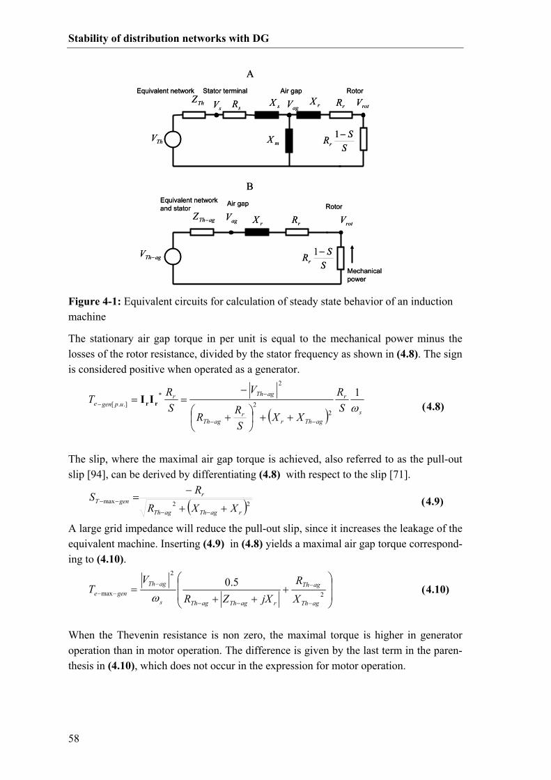
Stability of distribution networks with DG
58
The stationary air gap torque in per unit is equal to the mechanical power minus the losses of the rotor resistance, divided by the stator frequency as shown in (4.8). The sign is considered positive when operated as a generator.
( ) s
r
agThrr
agTh
agThrupgene S
R
XXSRR
V
SRT
ω1
22
2
*.].[
−−
−
−
++
+
−== rrII ( 4.8)
The slip, where the maximal air gap torque is achieved, also referred to as the pull-out slip [94], can be derived by differentiating (4.8) with respect to the slip [71].
( )22max
ragThagTh
rgenT
XXRRS
++
−=
−−
−− ( 4.9)
A large grid impedance will reduce the pull-out slip, since it increases the leakage of the equivalent machine. Inserting (4.9) in (4.8) yields a maximal air gap torque correspond-ing to (4.10).
+
++=
−
−
−−
−−− 2
2
max5.0
agTh
agTh
ragThagThs
agThgene X
R
jXZR
VT
ω ( 4.10)
When the Thevenin resistance is non zero, the maximal torque is higher in generator operation than in motor operation. The difference is given by the last term in the paren-thesis in (4.10), which does not occur in the expression for motor operation.
AStator terminal
ThV
ThZsX
mX
rX rREquivalent network
agThV −
agThZ − rX
SSRr
−1
Equivalent networkand stator
Air gap
sR
rRagVAir gap
rotV
Mechanical power
B
sV agV
SSRr
−1
rotVRotor
Rotor
AStator terminal
ThV
ThZsX
mX
rX rREquivalent network
agThV −
agThZ − rX
SSRr
−1
Equivalent networkand stator
Air gap
sR
rRagVAir gap
rotV
Mechanical power
B
sV agV
SSRr
−1
rotVRotor
Rotor
Figure 4-1: Equivalent circuits for calculation of steady state behavior of an induction machine

Stability of distribution networks with DG
59
The torque is proportional to the square of the Thevenin voltage and approximately to the reciprocal of the Thevenin impedance plus the rotor leakage reactance. Figure 4-2 shows torque versus rotor speed curves of the induction generator with the step up transformer defined in Table B-3 and Table B-4, page 179. A compensation capacitor of 1 MVAr which approximately corresponds to the full load reactive power consumption has been inserted at the low voltage side of the transformer. The short cir-cuit ratio and the X/R ratio are defined on the high voltage side of the step up trans-former. Similar results were reported in [95].
4.2.1.1 Mechanical model As described in [34] and later on several publications on the subject, the flexibility of the shaft of a wind turbine influences the behavior during and after a severe grid fault. The common way of representing the flexibility of a wind turbine is the two mass model in Figure 4-3. The turbine rotor and the generator rotor are represented as two lumped rotating masses with some stiffness and damping between them. The stiffness and the
A: Short Circuit Ratio B: X/R
C: Compensation Capacitor [MVAr] D: VTh [p.u.]
2
5
10
50
00.511.5
125
10
0.951.01.05
A: Short Circuit Ratio B: X/R
C: Compensation Capacitor [MVAr] D: VTh [p.u.]
2
5
10
50
00.511.5
125
10
0.951.01.05
Figure 4-2: Torque curves of an induction generator with step-up transformer. The following base case has been used: SCR = 10, X/R = 5, Qcap = 1 MVAr, VTh = 1 p.u. The four sub plots show the effects of deviations from the base case. In some of the cases, the stator voltage is outside the normal operation range.

Stability of distribution networks with DG
60
damping can be fine tuned based on estimation of the eigenfrequency and damping of shaft oscillations as shown on a real turbine in [96]. The gear box is usually considered as an ideal ratio, which is taken into account in the per unit conversion.
The motion of the system can be described with the four differential equations in (4.11) (4.14).
( ) ( )genrotorrateddampgenrotorstiffwindrotor
rotor KKTdt
dH ωωωθθ
ω−−−−=2 ( 4.11)
( ) ( )genrotorrateddampgenrotorstiffgengen
gen KKTdt
dH ωωωθθ
ω−+−+−=2 ( 4.12)
rotorratedrotor
dtd
ωωθ
= ( 4.13)
genratedgen
dtd
ωωθ
= ( 4.14)
The total momentum of the two rotating masses can be expressed with the equivalent or aggregated rotor speed in (4.15) and the equivalent inertia constant in (4.16) which ful-fill the differential equation in (4.17) [34]. Alternatively, the equivalent speed could be based on the total kinetic energy rather than the total momentum, but for a fixed speed wind turbine the difference is rather small.
genrotor
gengenrotorrotoreq HH
HH+
+=
ωωω ( 4.15)
genrotoreq HHH += ( 4.16)
genwindeq
eq TTdt
dH −=
ω2 ( 4.17)
Aerodynamic Turbine rotor Main shaft Generator rotor
⋅
radupKdamp
sec..
[ ].. upTwind
[ ]radrotor θ
[ ].. uprotorω [ ]secH gen
[ ]secH rotor
[ ]radupK stiff /.. [ ].. upTgen
[ ]radgen θ[ ].. upgenω
Generator fluxAerodynamic Turbine rotor Main shaft Generator rotor
⋅
radupKdamp
sec..
[ ].. upTwind
[ ]radrotor θ
[ ].. uprotorω [ ]secH gen
[ ]secH rotor
[ ]radupK stiff /.. [ ].. upTgen
[ ]radgen θ[ ].. upgenω
Generator flux
Figure 4-3: Mechanical model of the drive shaft in per unit.

Stability of distribution networks with DG
61
The time it takes before the equivalent rotor speed exceeds the point in Figure 4-2 whe-re the electrical torque is smaller than the mechanical torque can roughly be estimated with (4.18).
genwind
eqeq
TTH
t−
∆=∆
2ω ( 4.18)
For example, the wind turbine of Appendix B has a total inertia constant of 4 seconds. With a short circuit ratio of 5 and an X/R ratio of 5 like the dash-dotted line in Figure 4-2 A, the difference between the rotor speed at the rated power production and the maximal allowable rotor speed is approximately 0.03 p.u. Assuming that the torque from the wind is 1 p.u. and that the electrical braking torque during the fault is 0, the maximal fault clearing time according to (4.18) is 0.03 · 2 · 4 = 0.24 sec. This is, how-ever, a rather optimistic estimate, because it takes some time for the flux to recover after the fault is cleared and because the oscillation which is erected in the shaft combined with the non-linear torque characteristic results in a lower braking torque.
4.2.2 The influence of Danish concept wind turbines on the network parameters The presence of directly grid connected wind turbines affects the Thevenin parameters of the network in the vicinity. When performing a short circuit calculation, for example with PowerFactory®, an induction machine is typically represented as a constant volt-age behind a transient reactance, given by (4.19), and the stator resistance as depicted in Figure 4-4 A. The voltage represents the electromotive force corresponding to the flux linkage trapped in the rotor cage [71]. This means that the generator will supply reactive current to the network during a short circuit and thereby support the grid voltage. The rotor flux will, however, decay with a time constant which is comparable to the subtran-sient time constant of a synchronous machine. During a severe voltage dip, the braking torque of the generator is significantly reduced, which causes the rotor speed to in-crease. When the fault is cleared, the rotor must be decelerated down to its rated speed. The impact on the network after the fault can to some extend be analyzed by studying the steady state equivalent circuit in Figure 4-4 B, where the equivalent rotor resistance is given by the physical rotor impedance divided by the slip given in (4.21).
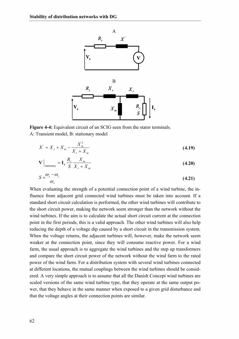
Stability of distribution networks with DG
62
mr
mms XX
XXXX
+−+=
2' ( 4.19)
mr
mr
XXX
SR
+= rIV
stationary
' ( 4.20)
s
rsSωωω −
= ( 4.21)
When evaluating the strength of a potential connection point of a wind turbine, the in-fluence from adjacent grid connected wind turbines must be taken into account. If a standard short circuit calculation is performed, the other wind turbines will contribute to the short circuit power, making the network seem stronger than the network without the wind turbines. If the aim is to calculate the actual short circuit current at the connection point in the first periods, this is a valid approach. The other wind turbines will also help reducing the depth of a voltage dip caused by a short circuit in the transmission system. When the voltage returns, the adjacent turbines will, however, make the network seem weaker at the connection point, since they will consume reactive power. For a wind farm, the usual approach is to aggregate the wind turbines and the step up transformers and compare the short circuit power of the network without the wind farm to the rated power of the wind farm. For a distribution system with several wind turbines connected at different locations, the mutual couplings between the wind turbines should be consid-ered. A very simple approach is to assume that all the Danish Concept wind turbines are scaled versions of the same wind turbine type, that they operate at the same output po-wer, that they behave in the same manner when exposed to a given grid disturbance and that the voltage angles at their connection points are similar.
A 'XsR
sV 'V
'XsR
sV 'V
B
sX
mX
rX
SRr
sR
sV rI
sX
mX
rX
SRr
sR
sV rI
Figure 4-4: Equivalent circuit of an SCIG seen from the stator terminals. A: Transient model, B: stationary model

Stability of distribution networks with DG
63
With these assumptions, an equivalent Thevenin impedance for a given wind turbine can be calculated according to (4.22). The idea is that the mutual impedances are scaled up according to the amount of wind power going through them.
[ ] [ ]∑≠ −
−− +≈
nm nrated
mratedmnnnnTh S
S,, II ZZZ ( 4.22)
Figure 4-5 shows a simplified equivalent circuit of two wind turbines connected to a strong network through a common line.
The equivalent Thevenin impedance of WT 1 calculated according to (4.22) is shown in (4.23).
ADADBDTh ZZZZ ⋅++≈−
−−
1
21
WTn
WTnWT S
S ( 4.23)
If ZBD and ZCD are very small compared to ZAD and the two wind turbines have the sa-me size, the short circuit power, seen from each of the turbines, is half the actual short circuit power of their connection points. This is equivalent to inserting of an up-scaled aggregated wind turbine while maintaining the original network parameters. On the other hand, if ZAD is very small, there will be only little cross coupling between the two wind turbines. If the X/R ratio of ZAD is different from the one of ZBD, the re-sulting X/R ratio at Bus B is also changed by the presence of WT 2.
4.2.2.1 Example As mentioned earlier, the equivalent short circuit power only gives a rough estimate of the strength of the network at a given connection point. To illustrate the application, a small example is simulated. Figure 4-6 shows the network used for loss allocation in Section 3.2.3 and 3.3.4, where the loads have been replaced with wind turbines. The parameters of the wind turbines and the wind turbine transformers can be found in Appendix B, page 179 ff. The basis for the investigation is the small wind farm, WT2, which comprises two 2 MW wind turbines. The effect of the connection of the wind farm with four 2 MW wind turbines either at Bus 3 or Bus 4 is investigated.
Figure 4-5: Equivalent circuit of a system with two wind turbines.
Bus A
Bus B
Bus C
Bus D
ZBD
ZCD
ZAD
WT1
WT2

Stability of distribution networks with DG
64
The Thevenin impedances of Bus 2 – 6 have been calculated in Table 3-2, page 49. The impedance of the external network has not been considered. The short circuit power at Bus 2 when disregarding all wind turbines can be calculated according to (4.5), page 56. Assuming that the Thevenin voltage is close to 1 p.u., the Short circuit power is given by (4.24) .
1.3 ,72.1551001.7287i 0.55781
12 =∠=⋅
−=− R
XMVAMVABusscoS ( 4.24)
When the wind farm at Bus 3 is connected as well, the mutual impedance between Bus 3 and Bus 2 must also be considered. This gives the expression in (4.25). Bus 2 and Bus 3 only share the 60 kV network and the 150/60 kV transformer. Therefore, the mu-tual impedance has a higher X/R ratio than the self-impedances of the two bus bars. The short circuit power at Bus 2 has been reduced with a factor of 1.6 and the installed wind power has been increased with a factor of 3.
( )
5.4 ,77.633
1000.63448i 0.051321.7287i 0.55781
132
=∠=
⋅−+−
=−−−
RXMVA
MVAWTBuseqsc
o
S ( 4.25)
8 MW 8 MW
4 MW
2 km 2 km
1 km 2 km 1 km
5 km
5 km
20 km
Equi
vale
nt o
f WT4
Equi
vale
nt o
f WT3
2-W
indi
ng..
G~
WT3
2-W
indi
ng..
G~
WT2
G~
WT4
2-W
indi
ng..
Line_7_10
Line_4_9Line_2_6Line_2_5Line_5_9
Line
_3_1
1
2-W
indi
ng..
2-W
indi
ng..
Line_8_10 Line_7_8
2-W
indi
ng..
External Grid
Bus3A
Bus2A
Bus4A
Bus4
Bus6Bus2
Bus3
Bus11
Bus10
Bus5
Bus9
Bus8
Bus7
Bus1
Figure 4-6: Example network for illustration of the influence of adjacent wind turbines on the short term voltage stability. The network is the same as in Figure 3-4 page 38.

Stability of distribution networks with DG
65
If the extra wind farm is placed at Bus 4 rather than Bus 3, the two wind farms share the 60/10 kV transformer plus a larger part of the 60 kV network. The equivalent short cir-cuit power for that case is given by (4.26). The equivalent X/R ratio is further increased, since an extra transformer is shared among the two wind farms. In this case the short circuit power is reduced with a factor of 2.75, and the wind capacity is still increased with a factor of 3.
( )
2.6 ,80.920
1001.6253i 0.1220621.7287i 0.55781
142
=∠=
⋅−+−
=−−−
RXMVA
MVAWTBuseqsc
o
S ( 4.26)
Figure 4-7 shows the results of five RMS fault simulations made with PowerFactory® where a three phase short circuit with duration of 100 ms is applied at Bus 1. In all the cases, the wind turbines are producing their rated power and they are full load compen-sated before the fault occurs. Case A shows a reference simulation where only WT 2 is active. Case B shows a simulation where both WT 2 and WT 3 are active. The voltage dip of Case B is not as deep as for Case A, since both wind turbines contribute with reactive power during the fault. After the fault is cleared, the voltage returns faster in case A than in Case B, since both wind turbines consume reactive power in that period. In case C, Line_2_5 has been opened, and the transformer, Equivalent of WT 3, with a short circuit power as specified in (4.25) has been activated. Therefore, WT 2 is simu-lated alone with the equivalent network impedance. It can be seen that curve B and C are very similar, especially in the beginning. During the short circuit, it is easier for WT 2 to hold the voltage when the impedance is higher, and after the fault the higher im-pedance delays the voltage recovery. Case D and E show the same simulations as case B and C only with WT4 active instead of WT 3. During the first 0.5 seconds after the fault has occurred the two simulations give similar results, but after that point there is some deviation between the two curves. The reason is that the fault clearing time of 100 ms is close to the critical fault clearing time for this system. This means that when the fault is cleared and the flux has returned in the machine, there is very little difference between the electrical and the mechanical torque. This means that the course of the state variables is very sensitive even to small parameter changes. With a fault clearing time of 75 ms, the two curves could hardly be distinguished.
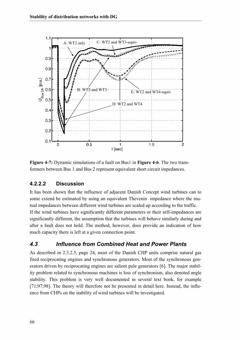
Stability of distribution networks with DG
66
4.2.2.2 Discussion It has been shown that the influence of adjacent Danish Concept wind turbines can to some extend be estimated by using an equivalent Thevenin impedance where the mu-tual impedances between different wind turbines are scaled up according to the traffic. If the wind turbines have significantly different parameters or their self-impedances are significantly different, the assumption that the turbines will behave similarly during and after a fault does not hold. The method, however, does provide an indication of how much capacity there is left at a given connection point.
4.3 Influence from Combined Heat and Power Plants As described in 2.3.2.5, page 24, most of the Danish CHP units comprise natural gas fired reciprocating engines and synchronous generators. Most of the synchronous gen-erators driven by reciprocating engines are salient pole generators [6]. The major stabil-ity problem related to synchronous machines is loss of synchronism, also denoted angle stability. This problem is very well documented in several text book, for example [71;97;98]. The theory will therefore not be presented in detail here. Instead, the influ-ence from CHPs on the stability of wind turbines will be investigated.
D: WT2 and WT4
A: WT2 only
E: WT2 and WT4-equivB: WT2 and WT3
C: WT2 and WT3-equiv
D: WT2 and WT4
A: WT2 only
E: WT2 and WT4-equivB: WT2 and WT3
C: WT2 and WT3-equiv
Figure 4-7: Dynamic simulations of a fault on Bus1 in Figure 4-6. The two trans-formers between Bus 1 and Bus 2 represent equivalent short circuit impedances.
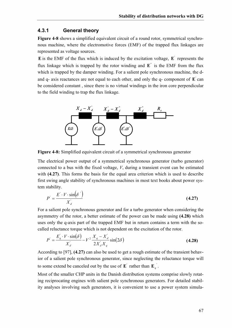
Stability of distribution networks with DG
67
4.3.1 General theory Figure 4-8 shows a simplified equivalent circuit of a round rotor, symmetrical synchro-nous machine, where the electromotive forces (EMF) of the trapped flux linkages are represented as voltage sources. E is the EMF of the flux which is induced by the excitation voltage, 'E represents the flux linkage which is trapped by the rotor winding and ''E is the EMF from the flux which is trapped by the damper winding. For a salient pole synchronous machine, the d- and q- axis reactances are not equal to each other, and only the q- component of 'E can be considered constant , since there is no virtual windings in the iron core perpendicular to the field winding to trap the flux linkage.
The electrical power output of a symmetrical synchronous generator (turbo generator) connected to a bus with the fixed voltage, V, during a transient event can be estimated with (4.27). This forms the basis for the equal area criterion which is used to describe first swing angle stability of synchronous machines in most text books about power sys-tem stability.
( )
'
''' sin
dXVE
Pδ⋅⋅
= ( 4.27)
For a salient pole synchronous generator and for a turbo generator when considering the asymmetry of the rotor, a better estimate of the power can be made using (4.28) which uses only the q-axis part of the trapped EMF but in return contains a term with the so-called reluctance torque which is not dependent on the excitation of the rotor.
( ) ( )δδ
2sin2
sin'
'2
'
''
qd
dq
d
q
XXXX
VX
VEP
−−
⋅⋅= ( 4.28)
According to [97], (4.27) can also be used to get a rough estimate of the transient behav-ior of a salient pole synchronous generator, since neglecting the reluctance torque will to some extend be canceled out by the use of 'E rather than '
qE .
Most of the smaller CHP units in the Danish distribution systems comprise slowly rotat-ing reciprocating engines with salient pole synchronous generators. For detailed stabil-ity analyses involving such generators, it is convenient to use a power system simula-
δ∠E
'dd XX − sR
' ' δ∠E ' ' '' δ∠E
'''dd XX − ''
dX
δ∠E
'dd XX − sR
' ' δ∠E ' ' '' δ∠E
'''dd XX − ''
dX
Figure 4-8: Simplified equivalent circuit of a symmetrical synchronous generator

Stability of distribution networks with DG
68
tion tool which is considers saliency, saturation, excitation system etc. The aim of this chapter is to give a more general understanding of the influence of CHP units on the stability of other units. Therefore, the saliency is neglected in the following. If a three phase short circuit occurs at the stator terminal of an unloaded synchronous machine, the fundamental frequency component of the current can be estimated with (4.29) where the first term denotes the stationary fault current under the assumption that the excitation voltage is kept constant, the second term denotes the current which will decay with the d-axis transient short circuit time constant '
dτ , which is usually in the
range of 0.5 to 3 seconds [98]. The Last term describes a current which is decaying with the d-axis subtransient short circuit time constant ''
dτ which is typically in the range of
0.02 to 0.05 s. Further, there will be a DC-component which will decay with the arma-ture time constant.
−+
−+⋅⋅=
−− '''
''''
11111dd
t
dd
t
ddd
eXX
eXXX
j ττEIsc ( 4.29)
If the short circuit does not occur right at the terminal of the synchronous generator, but at a given distance, not only the magnitude of the current, but also the equivalent time constants will be changed.
4.3.2 Influence of a synchronous machine on the Thevenin pa-rameters Using the assumption of a constant flux linkage, the influence of a synchronous genera-tor on the Thevenin impedance and voltage at a given connection point can be assessed by adding a virtual voltage source behind a transient or a sub transient reactance to the network equations (4.1) to (4.4), page 56ff. This is the same approach as the one used to assess the influence of a STATCOM or an SVC later in Section 4.4. There are, how-ever, some fundamental differences between FACTS devices like SVCs and STAT-COMS and a synchronous generator. Firstly, the synchronous generator is attached to a prime mover unit which enables the generator to deliver active power during a short circuit. In cases where the production before the fault was fairly high, the mechanical power from the prime mover will cause the rotor to accelerate, which changes the angle of the Thevenin voltages relative to the remaining network. Secondly, the damper wind-ing will behave like an induction generator. During the short circuit, the demagnetizing of the damper windings will cause the generator to inject reactive current. But after the fault is cleared, the magnetizing of the damper winding will cause an extra consumption of reactive power.
4.3.2.1 Example To illustrate the influence of a synchronous generator on the Thevenin parameters at a connection point and thereby the stability of an induction generator, the example from section 4.2.2.1, page 63 is revisited. The 4 MW two turbine wind farm at Bus 2 is kept,
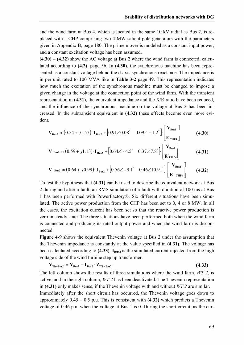
Stability of distribution networks with DG
69
and the wind farm at Bus 4, which is located in the same 10 kV radial as Bus 2, is re-placed with a CHP comprising two 4 MW salient pole generators with the parameters given in Appendix B, page 180. The prime mover is modeled as a constant input power, and a constant excitation voltage has been assumed. (4.30) – (4.32) show the AC voltage at Bus 2 where the wind farm is connected, calcu-lated according to (4.2), page 56. In (4.30), the synchronous machine has been repre-sented as a constant voltage behind the d-axis synchronous reactance. The impedance is in per unit rated to 100 MVA like in Table 3-2 page 49. This representation indicates how much the excitation of the synchronous machine must be changed to impose a given change in the voltage at the connection point of the wind farm. With the transient representation in (4.31), the equivalent impedance and the X/R ratio have been reduced, and the influence of the synchronous machine on the voltage at Bus 2 has been in-creased. In the subtransient equivalent in (4.32) these effects become even more evi-dent.
( ) [ ]
⋅−∠∠+⋅+≈ °°
CHP4
Bus1
Bus2Bus2E
VIV 2.10.0908.00.9157.154.0 j ( 4.30)
( ) [ ]
⋅∠∠+⋅+≈ °°
CHP4'
Bus1
Bus2Bus2
E
VIV 8.70.374.5-0.6413.159.0' j ( 4.31)
( ) [ ]
⋅∠∠+⋅+≈ °°
CHP4
Bus1
Bus2Bus2
E
VIV
' '
' ' 91.100.469.1-0.5699.064.0 j ( 4.32)
To test the hypothesis that (4.31) can be used to describe the equivalent network at Bus 2 during and after a fault, an RMS simulation of a fault with duration of 100 ms at Bus 1 has been performed with PowerFactory®. Six different situations have been simu-lated. The active power production from the CHP has been set to 0, 4 or 8 MW. In all the cases, the excitation current has been set so that the reactive power production is zero in steady state. The three situations have been performed both when the wind farm is connected and producing its rated output power and when the wind farm is discon-nected. Figure 4-9 shows the equivalent Thevenin voltage at Bus 2 under the assumption that the Thevenin impedance is constantly at the value specified in (4.31). The voltage has been calculated according to (4.33). IBus2 is the simulated current injected from the high voltage side of the wind turbine step up transformer. Bus2ThBus2Bus2Bus2Th ZIVV −− ⋅−= ( 4.33) The left column shows the results of three simulations where the wind farm, WT 2, is active, and in the right column, WT 2 has been deactivated. The Thevenin representation in (4.31) only makes sense, if the Thevenin voltage with and without WT 2 are similar. Immediately after the short circuit has occurred, the Thevenin voltage goes down to approximately 0.45 – 0.5 p.u. This is consistent with (4.32) which predicts a Thevenin voltage of 0.46 p.u. when the voltage at Bus 1 is 0. During the short circuit, as the cur-
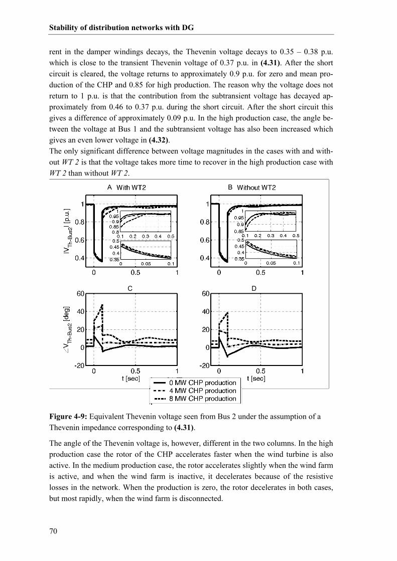
Stability of distribution networks with DG
70
rent in the damper windings decays, the Thevenin voltage decays to 0.35 – 0.38 p.u. which is close to the transient Thevenin voltage of 0.37 p.u. in (4.31). After the short circuit is cleared, the voltage returns to approximately 0.9 p.u. for zero and mean pro-duction of the CHP and 0.85 for high production. The reason why the voltage does not return to 1 p.u. is that the contribution from the subtransient voltage has decayed ap-proximately from 0.46 to 0.37 p.u. during the short circuit. After the short circuit this gives a difference of approximately 0.09 p.u. In the high production case, the angle be-tween the voltage at Bus 1 and the subtransient voltage has also been increased which gives an even lower voltage in (4.32). The only significant difference between voltage magnitudes in the cases with and with-out WT 2 is that the voltage takes more time to recover in the high production case with WT 2 than without WT 2.
The angle of the Thevenin voltage is, however, different in the two columns. In the high production case the rotor of the CHP accelerates faster when the wind turbine is also active. In the medium production case, the rotor accelerates slightly when the wind farm is active, and when the wind farm is inactive, it decelerates because of the resistive losses in the network. When the production is zero, the rotor decelerates in both cases, but most rapidly, when the wind farm is disconnected.
A B
C D
A B
C D
Figure 4-9: Equivalent Thevenin voltage seen from Bus 2 under the assumption of a Thevenin impedance corresponding to (4.31).
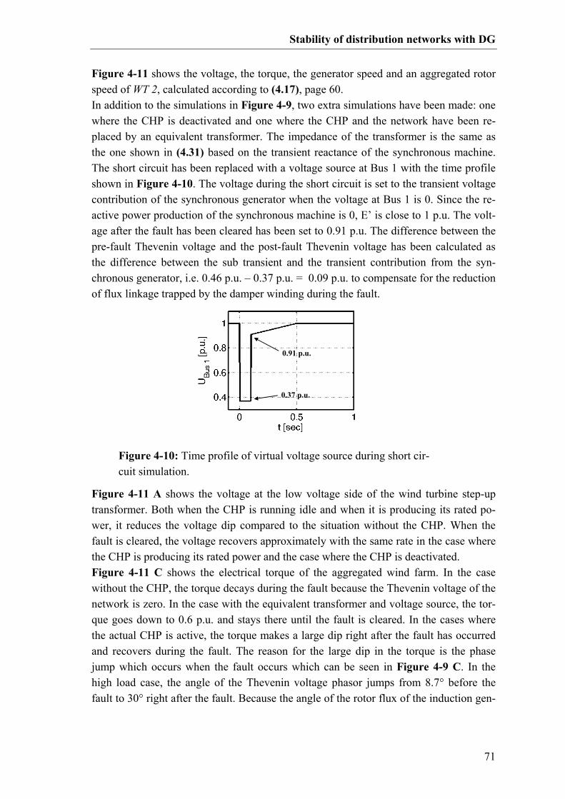
Stability of distribution networks with DG
71
Figure 4-11 shows the voltage, the torque, the generator speed and an aggregated rotor speed of WT 2, calculated according to (4.17), page 60. In addition to the simulations in Figure 4-9, two extra simulations have been made: one where the CHP is deactivated and one where the CHP and the network have been re-placed by an equivalent transformer. The impedance of the transformer is the same as the one shown in (4.31) based on the transient reactance of the synchronous machine. The short circuit has been replaced with a voltage source at Bus 1 with the time profile shown in Figure 4-10. The voltage during the short circuit is set to the transient voltage contribution of the synchronous generator when the voltage at Bus 1 is 0. Since the re-active power production of the synchronous machine is 0, E’ is close to 1 p.u. The volt-age after the fault has been cleared has been set to 0.91 p.u. The difference between the pre-fault Thevenin voltage and the post-fault Thevenin voltage has been calculated as the difference between the sub transient and the transient contribution from the syn-chronous generator, i.e. 0.46 p.u. – 0.37 p.u. = 0.09 p.u. to compensate for the reduction of flux linkage trapped by the damper winding during the fault.
Figure 4-11 A shows the voltage at the low voltage side of the wind turbine step-up transformer. Both when the CHP is running idle and when it is producing its rated po-wer, it reduces the voltage dip compared to the situation without the CHP. When the fault is cleared, the voltage recovers approximately with the same rate in the case where the CHP is producing its rated power and the case where the CHP is deactivated. Figure 4-11 C shows the electrical torque of the aggregated wind farm. In the case without the CHP, the torque decays during the fault because the Thevenin voltage of the network is zero. In the case with the equivalent transformer and voltage source, the tor-que goes down to 0.6 p.u. and stays there until the fault is cleared. In the cases where the actual CHP is active, the torque makes a large dip right after the fault has occurred and recovers during the fault. The reason for the large dip in the torque is the phase jump which occurs when the fault occurs which can be seen in Figure 4-9 C. In the high load case, the angle of the Thevenin voltage phasor jumps from 8.7° before the fault to 30° right after the fault. Because the angle of the rotor flux of the induction gen-
0.37 p.u.
0.91 p.u.
0.37 p.u.
0.91 p.u.
Figure 4-10: Time profile of virtual voltage source during short cir-cuit simulation.

Stability of distribution networks with DG
72
erator does not jump, the torque is reduced until the angle of the rotor flux has adjusted it self. When the fault is cleared, the phase makes a large negative jump in the cases where the CHP is active. This together with the increased rotor speed of the wind tur-bine generator creates a large positive torque impulse right after the fault is cleared. The aggregated rotor speed in Figure 4-11 D is a measure of the total mechanical momen-tum of the generator and the rotor of the wind turbine. The simulation with the equiva-lent transformer and voltage source predicts approximately the same rotor speed as the simulation where the CHP is running idle. The speed in the case where the CHP is pro-ducing its rated power is higher than the zero production case but still lower than in the case where the CHP is out of service.
The example has shown how an embedded CHP affects the Thevenin voltage and im-pedance during a short circuit in the transmission grid. It can be concluded that the pres-ence of a synchronous generator in the distribution system will always help making the voltage dip caused by a short circuit in the transmission system shallower. But apart from maintaining the voltage, the generator causes a phase angle jump when the fault occurs and when it is cleared. This effect is most evident when the generator has a high
A B
C D
A B
C D
Figure 4-11: State of WT 2 in Figure 4-6 after a short circuit in the transmission sys-tem with different configurations of the CHP at Bus 4.

Stability of distribution networks with DG
73
active power production. Due to the efficiency, most smaller CHP generators are either operated close to their rated power or taken out of service, which means that this effect cannot be neglected. Another property of smaller CHP units is that they tend to have a smaller inertia time constant than larger steam turbine units [6]. The inertia constant of the generator which was used in the example has an inertia constant, H, of 2 seconds. The model is taken from the standard library of PowerFactory®, but personal corre-spondence with Rolls Royce Marine® in Bergen has confirmed that the typical gensets with reciprocating gas engines which are used in Denmark have inertia constants of 1.5 to 2 seconds. For comparison, a typical large steam turbine typically has an inertia con-stant of 5-6 seconds [71]. Usually, large voltage phase jumps in the event of short circuits only occur when the X/R-ratio of the self impedance at the location of the short circuit is different from the X/R ratio of the mutual impedance between the connection point under consideration and the short circuit, which is usually the case when the short circuit occurs in the dis-tribution system [99]. It is shown that the representation in (4.31) where the synchronous generator is regarded as a constant voltage behind a transient reactance can be used to coarsely describe the influence, but when the CHP is producing its rated power, both the stationary rotor an-gle and the acceleration of the rotor during the fault must be taken into account. Further, the excitation system and the protection system of the generator should be considered. In the case study, the synchronous generator improves the transient voltage stability of the wind turbine, also at full production. It cannot generally be concluded that this will always be the case. In situations where the CHP is close to its angle stability limit in case of a fault, it could have a negative impact of the voltage stability margin of an ad-jacent wind farm. Because of the relatively small X/R ratios in the distribution systems, such an operation point would, however, lead to high thermal losses. It is therefore as-sumed that CHPs in most cases will have a positive impact on the transient voltage sta-bility of adjacent Danish concept wind turbines.
4.4 The influence of shunt compensation on network Thevenin parameters As described later in Chapter 5, shunt compensation units like SVCs and STATCOMS can be used to improve the power quality and the voltage profile in areas of the trans-mission system with high penetration of wind power and no adjacent power plants. In this section, it is shown, how a shunt compensation unit affects the equivalent short cir-cuit capacity at a connection point, and how this can improve the transient voltage sta-bility of a wind farm with Danish concept wind turbines. The SVC is modeled as a controllable susceptance with an upper limit of Bmax-SVC and a lower limit of Bmin-SVC. A more detailed description of the control and modeling of an SVC can be found in [100]. The control system is modeled as a droop controller with a

Stability of distribution networks with DG
74
droop of Xsl as shown in (4.34). A slower secondary voltage controller can be modeled with a change in the voltage set-point or a bias.
( )sl
comppointsetSVC XVVB 1
−= − ( 4.34)
When the voltage is close to 1 p.u. the current is close to the susceptance in p.u. This gives the reactive current, Iq-SVC, in (4.35).
( )sl
comppointsetSVCcompSVCq XVVBVI 1
−≈⋅= −− ( 4.35)
It follows that the ratio between a change in voltage and a change in reactive current is given by the droop constant. The STATCOM is modeled as a current controlled voltage source converter. The cur-rent magnitude is limited by the maximal current of the semiconductors. The control law for the reactive current of the STATCOM is given by (4.36).
( )sl
comppointsetSTATCOMq XVVI 1
−= −− ( 4.36)
Figure 4-12 shows a working diagram of an SVC and a STATCOM with the same rat-ing based on (4.35) and (4.36).
To illustrate the influence of the location and type of shunt compensation, a simplified example where an SVC or a STATCOM is placed somewhere along a long line is ana-lyzed. The simplified equivalent circuit in Figure 4-13 which represents a connection point at the end of a long line, has been analyzed. The line is represented by a series reactance with the value of Xgrid , and the voltage at the other end of the line is assumed to be constant. To increase the voltage stability at the connection point, a shunt compensation unit is placed somewhere along the line. k which is between 0 and 1, represents the relative electrical distance between the main grid and the shunt compensation unit.
slXI ⋅∆
I∆
V
qI
I∆
SVCmaxBI
−
∆
SVCminBI
−
∆I∆
STATCOMqI −−min
STATCOMqI −−max
pointsetV −
slXI ⋅∆
I∆
V
qI
I∆
SVCmaxBI
−
∆
SVCminBI
−
∆I∆
STATCOMqI −−min
STATCOMqI −−max
pointsetV −
Figure 4-12: Simplified working diagram of an SVC and a STATCOM with the same rating

Stability of distribution networks with DG
75
4.4.1 Shunt compensation unit as voltage controller When the shunt compensation unit is not operating at its limit, it controls the voltage according to (4.35) or (4.36). Since the current of the compensation unit is proportional to the difference between the set-point voltage and the actual voltage divided by the droop factor, the unit has been represented by a voltage source with a voltage corre-sponding to the set-point behind a reactance corresponding to the droop factor [73]. It should be noted that this does not reflect the actual electrical connection. Inserting the circuit in (4.1) - (4.5) and setting BSVC and Iq-STATCOM to zero yields a Thevenin imped-ance, Thevenin voltage and short circuit power corresponding to (4.37) to (4.39).
( )
grid
sl
slgrid
XX
k
XkkXj
+
+−=−
2
volt_contThZ ( 4.37)
slgrid
gridpointset
slgrid
slgrid
XkXXkV
XkXXV
+
⋅⋅+
+= −
−volt_contThV ( 4.38)
( ) nominal
slgrid
pointsetgridgrid
sl
VXkkX
kVVXX
j+−
+
=−
− 1volt_contSCS ( 4.39)
The closer the compensation unit gets to the connection point and the lower the control-ler droop gets, the lower the Thevenin impedance gets, and the higher the short circuit power gets. It should be noted that in case of a short circuit in the vicinity, the compen-sation unit would not be able to deliver the short circuit power in (4.39), since it would reach its capacity limit and because it is not able to supply active power. The short cir-cuit power is therefore only a measure of the strength of the network for small signal analysis. The Thevenin voltage is a weighted average of the grid voltage and the voltage set point. When adding the voltages, the phase must be considered. Therefore, the The-venin voltage and the short circuit power are in principle dependent on the loading of the system.
gridkX
SVCB
( ) gridXk−1
gridVconV
compV
V STATCOMqI −I
VpointsetV −
slXA B C
gridkX
SVCBSVCB
( ) gridXk−1
gridVconV
compV
VV STATCOMqI −I
VpointsetV −
slX
VVpointsetV −
slXA B C
Figure 4-13: simple grid for illustration of the influence for shunt compensation. A: Compensation unit in linear control region, B: SVC at susceptance limit, C: STAT-COM at current limit

Stability of distribution networks with DG
76
4.4.2 Shunt compensation unit in limitation If the compensation unit is not able to supply enough reactive power to maintain the voltage, it will change its control scheme. An SVC will in this case behave like a ca-pacitor, and a STATCOM will behave like a current source, provided that they are able to stay connected during the perturbation. Inserting the network in (4.1) - (4.5), the Thevenin parameters can be expressed as (4.40) – (4.42) When the compensation unit is an SVC, Iq-STATCOM is zero, and for a STATCOM BSVC is zero.
( )( )
gridSVC
gridSVCgrid
XBkkkXBX
j⋅−
+−=− 1
12
limitThZ ( 4.40)
gridSVC
STATCOMqgridgrid
XBkIXjkV
⋅−
⋅−= −
− 1limitThV ( 4.41)
( )( ) nominalgridSVCgrid
STATCOMqgridgrid VkkXBX
IXkVj12 +−
⋅−⋅= −
−limitscS ( 4.42)
Figure 4-14 shows an example of the dependency of the Thevenin parameters on the location and type of the shunt compensation unit when the compensation unit is operat-ing at its capacity limit.
In the SVC case, the Thevenin impedance is dependent on the location of the unit. For values of Bcomp which are positive and smaller than 1/ Xgrid the Thevenin impedance will increase when k is increased, i.e. the compensation unit is moved closer to the con-nection point. The same applies for the Thevenin voltage. When the SVC is located at the connection point or in the far end of the line, it has no influence on the short circuit
A: SVC
B: STATCOM
ThV
SCS
ThX
ThV
SCS
ThX
A: SVC
B: STATCOM
ThV
SCS
ThX
ThV
SCS
ThX
Figure 4-14: Thevenin parameters of the grid in Figure 4-13 when the compensation unit has reached its capacity limit. Xgrid = 0.5 p.u. Vgrid = 1 p.u., Bcomp = 0.8 p.u. and Icomp = -j0.8 p.u.
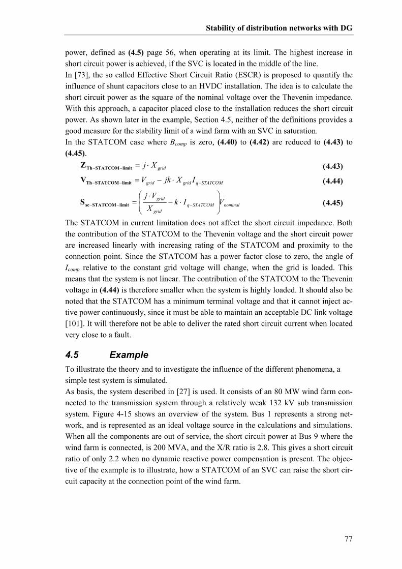
Stability of distribution networks with DG
77
power, defined as (4.5) page 56, when operating at its limit. The highest increase in short circuit power is achieved, if the SVC is located in the middle of the line. In [73], the so called Effective Short Circuit Ratio (ESCR) is proposed to quantify the influence of shunt capacitors close to an HVDC installation. The idea is to calculate the short circuit power as the square of the nominal voltage over the Thevenin impedance. With this approach, a capacitor placed close to the installation reduces the short circuit power. As shown later in the example, Section 4.5, neither of the definitions provides a good measure for the stability limit of a wind farm with an SVC in saturation. In the STATCOM case where Bcomp is zero, (4.40) to (4.42) are reduced to (4.43) to (4.45). gridXj ⋅=−− limitSTATCOMThZ ( 4.43)
STATCOMqgridgrid IXjkV −−− ⋅−=limitSTATCOMThV ( 4.44)
nominalSTATCOMqgrid
grid VIkX
Vj
⋅−
⋅= −−− limitSTATCOMscS ( 4.45)
The STATCOM in current limitation does not affect the short circuit impedance. Both the contribution of the STATCOM to the Thevenin voltage and the short circuit power are increased linearly with increasing rating of the STATCOM and proximity to the connection point. Since the STATCOM has a power factor close to zero, the angle of Icomp relative to the constant grid voltage will change, when the grid is loaded. This means that the system is not linear. The contribution of the STATCOM to the Thevenin voltage in (4.44) is therefore smaller when the system is highly loaded. It should also be noted that the STATCOM has a minimum terminal voltage and that it cannot inject ac-tive power continuously, since it must be able to maintain an acceptable DC link voltage [101]. It will therefore not be able to deliver the rated short circuit current when located very close to a fault.
4.5 Example To illustrate the theory and to investigate the influence of the different phenomena, a simple test system is simulated. As basis, the system described in [27] is used. It consists of an 80 MW wind farm con-nected to the transmission system through a relatively weak 132 kV sub transmission system. Figure 4-15 shows an overview of the system. Bus 1 represents a strong net-work, and is represented as an ideal voltage source in the calculations and simulations. When all the components are out of service, the short circuit power at Bus 9 where the wind farm is connected, is 200 MVA, and the X/R ratio is 2.8. This gives a short circuit ratio of only 2.2 when no dynamic reactive power compensation is present. The objec-tive of the example is to illustrate, how a STATCOM of an SVC can raise the short cir-cuit capacity at the connection point of the wind farm.

Stability of distribution networks with DG
78
4.5.1 The components
4.5.1.1 Wind farm The wind farm is modeled as an aggregation of forty 2 MW Danish Concept wind tur-bines similar to one presented in [89;102]. The parameters are given in Appendix B, page 179. RMS simulations have been made with PowerFactory® both using a two-mass model and a lumped rotor model. Due to a different structure of the used models, the wind power has been represented by a fixed mechanical power input during the simulations with the lumped rotor model and as a constant mechanical torque during simulations with the two-mass model. The local phase compensating capacitor is assumed to have a constant capacity during the simulation.
4.5.1.2 STATCOM The STACTOM has been modeled as a 40 MVA current controlled voltage source in-verter behind a filter reactance. The active power losses of the converter have not been considered. In normal operation, the d-axis current is used to control the voltage of the
Figure 4-15: Single line diagram of the test system

Stability of distribution networks with DG
79
DC-link capacitor, and the q-axis current is used to control the AC voltage magnitude. When the rated current is reached, the current magnitude is limited. In the steady state analysis, the STATCOM is either considered a voltage source behind a reactance corre-sponding to the controller droop or a current source which injects the rated current with a power factor of 0. The control law is given by the simple controller in (4.46) where the current is in p.u. with 40 MVA base, and s is the Laplace operator.
( ) ( )sXVVI
slpointsetmeasrefq 05.01
1+
−= −− ( 4.46)
4.5.1.3 SVC The SVC is modeled as a fixed 40 MVAr capacitor and a thyristor controlled reactor. The firing angle is used to control the voltage. When the firing angle reaches 180° the SVC will behave like a fixed capacitor. For the steady state calculations, the SVC is either considered a voltage source behind a reactance corresponding to the controller droop or a capacitor. The controller of the SVC is implemented according to (4.47) where the susceptance is in p.u. with 40 MVA as base. The firing angle is controlled by the standard interface of PowerFactory ®.
( ) ( )sXVVB
slmeaspointsetSVC 05.01
1+
−= − ( 4.47)
4.5.1.4 Load The local load at Bus 8 has in this case been modeled as a purely resistive load with a rated power of 50 MW.
4.5.1.5 Transformers The tap changers, saturation and magnetizing current of the transformers have not been considered.
4.5.2 Steady state analysis The objective of the analysis is to compare compensation with a STATCOM to com-pensation with an SVC, to compare dynamic compensation at the collection point (Bus 9) with dynamic compensation at the point of common coupling (Bus 6) and to investi-gate the influence of the controller droop. To make a systematic comparison, the 9 cases in Table 4-1 are investigated. In all the cases, a 44 MVAr capacitor corresponding to full load compensation of the generator and step up transformer at the nominal produc-tion is placed at the aggregated wind turbine generator (Bus 10). This compensation would in a typical application consist of a battery of switchable capacitors. Further, a 10 MVAr capacitor is placed at the point of common coupling (Bus 6), which ensures a voltage of 1 p.u. there at the nominal operation of the wind farm. This means that in steady state at the rated production, the dynamic compensation units do not provide any reactive power.

Stability of distribution networks with DG
80
4.5.2.1 Calculation of Thevenin parameters The Thevenin parameters for the situation where the wind farm is producing its rated power and is full load compensated have been calculated using (4.1) to (4.5), page 56 ff. The induction generator has been represented according to Figure 4-1 A with a slip of zero, which means that the Thevenin voltage denotes the bus voltage at a production of zero and the given compensation. Table 4-2 shows the calculated Thevenin parameters and an equivalent short circuit power at the generator terminals for the 9 cases. Slipmax denotes the maximal slip where the electrical braking power exceeds the nominal power of the wind farm. For the cases with voltage control, this point cannot be reached within the capacity limit. In the following, the slip is considered positive at super synchronous operation.
Case: Description
1 No dynamic compensation 2 An SVC or a STATCOM is controlling the voltage at the collection
point (Bus 9) and Xsl = 5% 3 An SVC or a STATCOM is controlling the voltage at the collection
point (Bus 9) and Xsl = 2% 4 An SVC is operating in susceptance limitation at
the collection point (Bus 9) 5 A STATCOM is operating in current limitation at
the collection point (Bus 9) 6 An SVC or a STATCOM is controlling the voltage at the point of
common coupling (Bus 6) and Xsl = 5% 7 An SVC or a STATCOM is controlling the voltage at the point of
common coupling (Bus 6) and Xsl = 2% 8 An SVC is operating in susceptance limitation at
at the point of common coupling (Bus 6) 9 A STATCOM is operating in current limitation at the point of common
coupling (Bus 6)
Table 4-1: Cases for stationary calculations
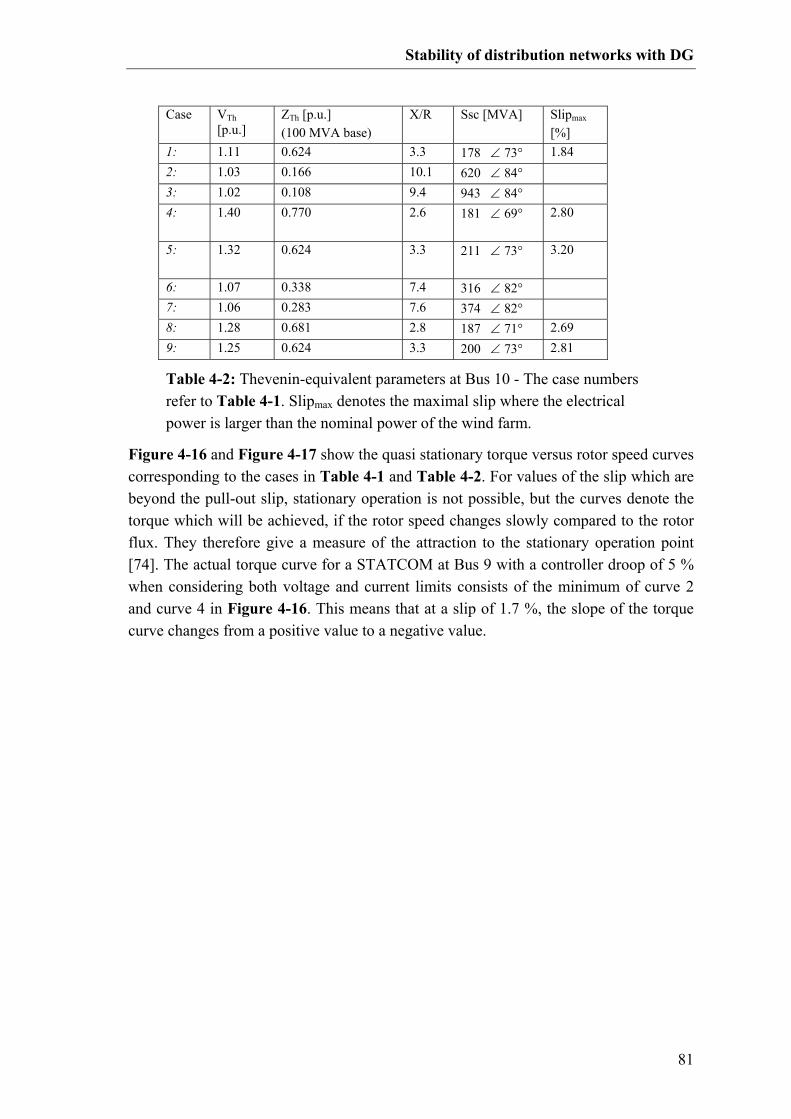
Stability of distribution networks with DG
81
Figure 4-16 and Figure 4-17 show the quasi stationary torque versus rotor speed curves corresponding to the cases in Table 4-1 and Table 4-2. For values of the slip which are beyond the pull-out slip, stationary operation is not possible, but the curves denote the torque which will be achieved, if the rotor speed changes slowly compared to the rotor flux. They therefore give a measure of the attraction to the stationary operation point [74]. The actual torque curve for a STATCOM at Bus 9 with a controller droop of 5 % when considering both voltage and current limits consists of the minimum of curve 2 and curve 4 in Figure 4-16. This means that at a slip of 1.7 %, the slope of the torque curve changes from a positive value to a negative value.
Case VTh
[p.u.] ZTh [p.u.] (100 MVA base)
X/R Ssc [MVA] Slipmax [%]
1: 1.11 0.624 3.3 178 ∠ 73° 1.84 2: 1.03 0.166 10.1 620 ∠ 84° 3: 1.02 0.108 9.4 943 ∠ 84° 4:
1.40 0.770 2.6 181 ∠ 69° 2.80
5:
1.32 0.624 3.3 211 ∠ 73° 3.20
6: 1.07 0.338 7.4 316 ∠ 82° 7: 1.06 0.283 7.6 374 ∠ 82° 8: 1.28 0.681 2.8 187 ∠ 71° 2.69 9: 1.25 0.624 3.3 200 ∠ 73° 2.81
Table 4-2: Thevenin-equivalent parameters at Bus 10 - The case numbers refer to Table 4-1. Slipmax denotes the maximal slip where the electrical power is larger than the nominal power of the wind farm.
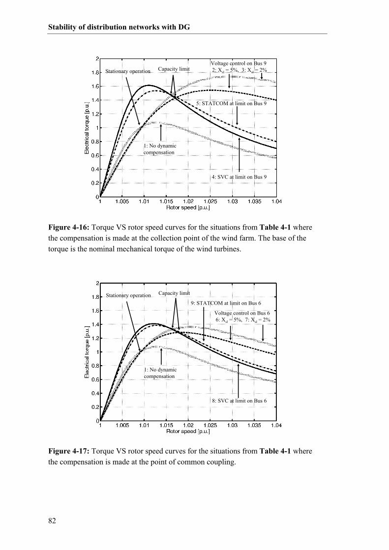
Stability of distribution networks with DG
82
1: No dynamic compensation
5: STATCOM at limit on Bus 9
4: SVC at limit on Bus 9
Voltage control on Bus 92: Xsl = 5%, 3: Xsl = 2%Stationary operation Capacity limit
1: No dynamic compensation
5: STATCOM at limit on Bus 9
4: SVC at limit on Bus 9
Voltage control on Bus 92: Xsl = 5%, 3: Xsl = 2%Stationary operation Capacity limit
Figure 4-16: Torque VS rotor speed curves for the situations from Table 4-1 where the compensation is made at the collection point of the wind farm. The base of the torque is the nominal mechanical torque of the wind turbines.
1: No dynamic compensation
9: STATCOM at limit on Bus 6
8: SVC at limit on Bus 6
Voltage control on Bus 66: Xsl = 5%, 7: Xsl = 2%
Stationary operation Capacity limit
1: No dynamic compensation
9: STATCOM at limit on Bus 6
8: SVC at limit on Bus 6
Voltage control on Bus 66: Xsl = 5%, 7: Xsl = 2%
Stationary operation Capacity limit
Figure 4-17: Torque VS rotor speed curves for the situations from Table 4-1 where the compensation is made at the point of common coupling.

Stability of distribution networks with DG
83
As described earlier, the contribution from the STATCOM to the Thevenin voltage at the connection point is dependent on the angle of the voltage where the STATCOM is connected. By inserting the network parameters in (4.4), page 56, the expression for the Thevenin voltage in (4.48) is derived. Bus6Bus9Bus1Bus10Th I6.680.37I5.7256.0V3.1111.1E ⋅°∠+⋅°∠+⋅°−∠=− ( 4.48) Since the current of the STATCOM is lagging the voltage with 90° when it is producing reactive power, the maximum contribution from a STATCOM at Bus 9 is achieved when the voltage angle at Bus 9 is -11.3° - 72.5° + 90° = 6.2°. Maximum contribution from a STATCOM at Bus 6 is achieved when the angle at Bus 6 is 10°. Figure 4-18 A shows the angle at Bus 9 when a 40 MVA STATCOM at its current limit is placed the-re. Figure 4-18 B shows that the corresponding Thevenin voltage at Bus 9 only varies with 1 % when the slip is varied between 0 and 20 %. Figure 4-18 C and D show that the same applies when the SVC is located at Bus 6.
Regarding the voltage magnitude, it is therefore a fair assumption to represent this net-work as a Thevenin-equivalent voltage behind a Thevenin-equivalent impedance, when a STATCOM is operating in current limit on Bus 6 or Bus 9.
A B
C D
A B
C D
Figure 4-18: The dependency of the Thevenin voltage on the loading of the system. A and B: STATCOM at current limit on Bus 9. C and D: STATCOM at current limit on Bus 6
Stability of distribution networks with DG
84
4.5.2.2 The influence of controller droop In the cases where the compensation unit is not at its limit, the droop, Xsl, has been set to either 2 % or 5 %. It follows from case 2, 3, 6 and 7 in Table 4-2, Figure 4-16 and Figure 4-17 that the influence of the droop setting is most evident, when the compensa-tion unit is located close to the connection point. The effect of decreasing the droop is that the steepness of the torque / slip curve is increased. The change in strength of the grid can be seen from the equivalent short circuit power. Where the system without dy-namic phase compensation only has a short circuit power of 178 MVA which gives a short circuit ratio of 1.9 at the low voltage side of the transformer, the system with shunt compensation unit at Bus 9 with a droop of 2 % has a short circuit power of 943 MVA and a short circuit ratio of 10.
4.5.2.3 STATCOM V.S. SVC When the output from the SVC or the STATCOM reaches its limit, the slip is in all the cases beyond the pull-out slip. The torque curves corresponding to the SVCs decay faster than those corresponding to the STATCOMs. The difference is most evident when the compensation unit is placed on Bus 9 which is close to the wind farm, and when the slip is very high. The reason is that the closer to the wind farm the SVC is located, the higher the Thevenin impedance at the connection point gets, where as the location of the STATCOM does not affect the impedance. As seen in (4.9), page 58, the Thevenin voltage only scales the Torque cur-ve, but the Thevenin impedance changes the shape. A high Thevenin impedance leads to a low pull-out slip which can be seen in Figure 4-16 curve 5. The maximal slip whe-re the electrical torque exceeds the mechanical torque under assumption of a constant mechanical power is highest in the case with a STATCOM on Bus 9 and lowest when an SVC is located on Bus 6. An SVC located on Bus 9 and a STATCOM located at Bus 6 result in the same critical rotor speed. The equivalent short circuit power calculated with (4.5) does not give an indication of which of the curves that has the largest critical rotor speed.
4.5.3 Calculation of Short circuit power using PowerFactory® In many cases, a model of the grid connection is available in a power system simulation tool. It is therefore convenient to use the tool to derive the Thevenin-equivalent parame-ters. For comparison with the directly calculated parameters, the Thevenin impedance, the Thevenin voltage and the short circuit power have been calculated with the station-ary short circuit analysis tool of PowerFactory® Version 13.1 Build 260. The complete calculation method uses algorithms which are similar to those used to calculate the data in Table 4-2. The outcome should therefore also be similar. The voltage source converter which has been used to model the STATCOM in the dy-namic simulation has two modes for short circuit calculations. Either it is considered a constant current source, delivering the pre fault current or a voltage source behind its

Stability of distribution networks with DG
85
filter reactance delivering the pre fault voltage. To model the behavior of a STATCOM or an SVC in the linear control mode, it has been replaced by a voltage source with a voltage of 1 p.u. and a power factor of zero behind a reactance with a size in p.u. corre-sponding to the controller droop. To emulate the STATCOM in current limitation, the STATCOM has been replaced by an ideal current source with an output corresponding to the rated current and a power factor of 0. To emulate the SVC in susceptance limit, it has been replaced by a 40 MVAr capacitor. The compensation locally on Bus 10 does not affect the short circuit power, but it does affect the X/R ratio and the Thevenin volt-age. In the calculations in Table 4-2, the generator is represented as a shunt impedance corresponding to the no-load situation. To get the same result in PowerFactory®, the reactive no load losses of the generator have been subtracted from the capacitor. In all the cases from Table 4-2 the output from PowerFactory ® deviates less than 1 % from the values calculated directly from the impedance matrix.
4.5.4 Dynamic simulation To visualize the effect of the different compensation types and locations on the stability of a wind farm, the 4 situations listed in Table 4-3 have been simulated. In all the simu-lations, the wind farm is producing its rated power, 80 MW, when a three-phase short circuit occurs on Bus 5. The controller droop of the SVC or the STATCOM is in all the situations set to 5 %.
To focus on the influence of the stationary torque curves on the stability limit, the simu-lations are firstly made with a representation of the wind turbine and generator rotor as one lumped mass. Secondly, simulations where the generator is represented as a two-mass model, as described in [89], are performed for comparison. All the simulations are performed using the RMS method, where only the fundamental frequency is considered [44].
4.5.4.1 Single-mass model In the simulations with a lumped rotor model, the fault clearing time is set to 150 ms to get the system close to the stability limit. Figure 4-19 shows the electrical torque, the mechanical torque and the relevant station-ary torque curves from Figure 4-16 and Figure 4-17 plotted against the rotor speed of the aggregated wind farm. The voltage magnitudes at Bus 6, 9 and 10 are depicted in
Case: Description
A 40 MVA STATCOM on Bus6 B 40 MVA STATCOM on Bus9 C 40 MVAr SVC on Bus6 D 40 MVAr SVC on Bus9
Table 4-3: Cases for dynamic fault simulations.

Stability of distribution networks with DG
86
Figure 4-20. The system is stable, when the electrical torque exceeds the mechanical torque after the fault is cleared and the rotor flux is restored. In case C where the SVC is placed at the point of common coupling, the slip is margin-ally above the critical point from Table 4-2 when the flux has reached its stationary value. Therefore, the wind turbines eventually overspeed. If the fault were cleared after 140 ms, this configuration would have been stable as well. In case A and D, the system is stable, but the maximal rotor speed is close to the critical value, where as in case B, there is a larger margin to the critical point. During the deceleration of the rotor, the torque does not follow the stationary torque curves, since there is a lag between the change in rotor speed and the change in rotor flux [94]. When the speed returns to the stationary point, there is a poorer damping of the electromechanical oscillations in case B and D, where the compensation is performed close to the wind farm, than in case A. The same simulation with a fault clearing time of 140 ms shows that the SVC on Bus 6 results in the same damping as the STATCOM on Bus 6. One explanation is that the Thevenin impedance when the compensation unit is in the linear control region is smaller in case B and D than in case A and C, which affects the eigenvalue with the lowest damping. This subject is treated in [103].
6
9
Mech. Torque
6
8 4
5
2
2
6
9
Mech. Torque
6
8 4
5
2
2
Figure 4-19: Electrical torque versus rotor speed rated after the rated torque of the wind farm. The numbered curves are the same as in Table 4-1

Stability of distribution networks with DG
87
To sum up, the largest stability margin in this simplified case is achieved with a STAT-COM at the collection point of the wind farm (Bus 9). A STATCOM at the point of common coupling (Bus 6) has approximately the same effect on the stability as an SVC at the collection point (Bus 9), and an SVC at the point of common coupling (Bus 6) provides the poorest stability margin. This ranking corresponds to the ranking of Slipmax
in Table 4-2. The damping of the electromechanical oscillations close to the rated operation is highest when the compensation unit is placed at the point of common coupling (Bus 6).
4.5.4.2 Two-mass model A real wind turbine has some flexibility in the shaft, which influences the stability limit of the system. A thorough description of this problem is found in [34]. Due to the extra energy storage in the flexible shaft, the stability limit cannot be illus-trated as simply as in the lumped rotor case. However, the Thevenin impedance and the Thevenin voltage and thereby the shape of the stationary torque curves still influence the stability. The same four simulations have been repeated with the two-mass model and a fault clearing time of 90 ms. Figure 4-21 shows the torque versus rotor speed plots for this situation. Instead of the rotor speed of the generator, the equivalent rotor speed, ωeq,
Figure 4-20: The voltage magnitudes at Bus 6, 9 and 10 at a fault on Bus 5 at t=0 s which is cleared at t=0.15 s.
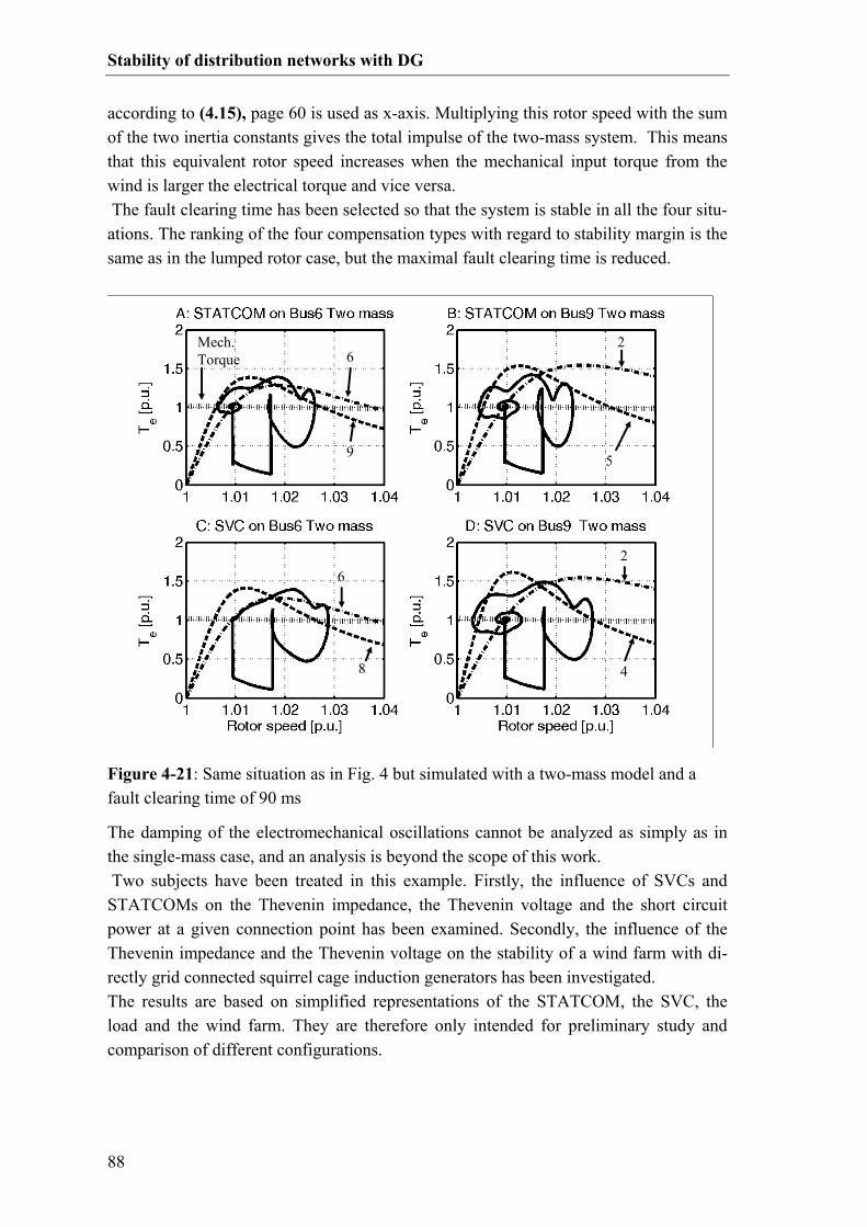
Stability of distribution networks with DG
88
according to (4.15), page 60 is used as x-axis. Multiplying this rotor speed with the sum of the two inertia constants gives the total impulse of the two-mass system. This means that this equivalent rotor speed increases when the mechanical input torque from the wind is larger the electrical torque and vice versa. The fault clearing time has been selected so that the system is stable in all the four situ-ations. The ranking of the four compensation types with regard to stability margin is the same as in the lumped rotor case, but the maximal fault clearing time is reduced.
The damping of the electromechanical oscillations cannot be analyzed as simply as in the single-mass case, and an analysis is beyond the scope of this work. Two subjects have been treated in this example. Firstly, the influence of SVCs and STATCOMs on the Thevenin impedance, the Thevenin voltage and the short circuit power at a given connection point has been examined. Secondly, the influence of the Thevenin impedance and the Thevenin voltage on the stability of a wind farm with di-rectly grid connected squirrel cage induction generators has been investigated. The results are based on simplified representations of the STATCOM, the SVC, the load and the wind farm. They are therefore only intended for preliminary study and comparison of different configurations.
6
9
Mech. Torque
6
8 4
5
2
2
6
9
Mech. Torque
6
8 4
5
2
2
Figure 4-21: Same situation as in Fig. 4 but simulated with a two-mass model and a fault clearing time of 90 ms

Stability of distribution networks with DG
89
4.6 Summary / discussion In this chapter, it has been investigated which factors affect the short term voltage sta-bility in a distribution network with distributed generation when it is exposed to a fault in the transmission system. The investigation has been split in two parts. Firstly the effect of the short circuit power, the X/R ratio, the Thevenin voltage and the local phase compensation on the stability margin of a Danish concept wind turbine has been described. Secondly, the influence of adjacent Danish concept wind turbines, CHPs, SVCs and STATCOMs on the Thevenin parameters at a connection point has been examined.
4.6.1 The influence of network parameters on the stability of Danish concept wind turbines The following main observations have been made:
• A low short circuit ratio at the connection point causes a low pull out torque and a low pull-out slip.
• A low X/R-ratio at the connection point causes a high pull out torque and a high pull-out slip.
• Local capacitive phase compensation increases the pull-out torque and slightly decreases the pull-out slip.
• The entire torque curve is scaled according to the square of the Thevenin volt-age.
The results are not considered new, but they are used to evaluate the influence of other production and compensation units on the stability limit.
4.6.2 The influence of adjacent wind turbines on the network parameters For the adjacent Danish concept turbines, it is concluded that the effect on a given Dan-ish concept wind turbine can be estimated by scaling up the mutual short circuit imped-ances according to the relative traffic of wind power going through them. This finding is considered new.
4.6.3 The influence from synchronous generators The influence of a synchronous generator running at no load can to some extend be compared to the influence of a constant voltage source behind a transient reactance. When the synchronous generator is highly loaded, this approach is still valid, but the rotor angle should be taken into account which causes positive voltage phase jump when a fault occurs, a negative phase jump when the fault is cleared and a smaller con-tribution to the voltage after the fault is cleared.
Stability of distribution networks with DG
90
4.6.3.1 The influence of STATCOMS and SVCs It is concluded that a STATCOM or an SVC operating in its linear control region has the effect that the Thevenin impedance at the connection point is reduced, the Thevenin voltage goes towards the set point voltage and the equivalent short circuit power is in-creased. These effects are more evident the closer to the connection point the unit is located and the lower the controller droop is. When an SVC reaches its capacity limit, it can be represented as a capacitor. The effect is that the Thevenin impedance and the Thevenin voltage at the connection point are increased, compared to the uncompensated situation. A STATCOM at its capacity limit can be represented as a current source. It will there-fore not affect the Thevenin impedance. Strictly speaking, a network with a STATCOM cannot be represented as a Thevenin equivalent, since the angle of the current injection is dependent on the loading of the system. In the study case it was, however, shown that the equivalent Thevenin voltage varied less than 1 % under the give circumstances. The contribution of the STATCOM to the Thevenin voltage is higher the closer to the con-nection point it is located. In situations where a STATCOM or an SVC is operating at its limit, the equivalent short circuit power including the compensation device is not considered a good measure of the equivalent strength of the network. It is concluded that the specification of a The-venin impedance and voltage provides more information about the nature of the network in these cases. It has been shown that the calculation of the Thevenin parameters can either be made based on the impedance matrix of the network or using a stationary short circuit calcula-tion tool, provided that it is able to consider current sources and capacitors.
4.6.3.2 The influence of dynamic compensation on a wind farm with SCIGs It is concluded that a good measure of the transient stability limit of a squirrel cage in-duction generator is the maximal rotor speed where the electrical braking power is higher than the rated mechanical input power. This value can be used to rate different solutions against each other, but not for a direct estimation of the maximal fault clearing time, since the rotor flux dynamics, and the effect of a flexible shaft will also affect the maximal fault clearing time. Given the Thevenin impedance and voltage at a connection point, both when the com-pensation devices are operating in their linear control region and when they are operat-ing at their capacity limits, the quasi stationary torque curves can easily be calculated for different generator types. The capacity limits of the shunt compensation unit can be found from the intersection between the two torque curves. For a given generator type, an increase in Thevenin impedance at the connection point will result in a lower pull-out slip and a lower maximal torque. When a STATCOM reaches its capacity limit, the resulting torque characteristic will therefore have the same

Stability of distribution networks with DG
91
shape as the characteristic without compensation, but scaled with a factor. An SVC at its limit will reduce the pull-out slip and thereby cause a torque curve which decays faster at higher slips than in the STATCOM case.


93
5 VOLTAGE/VAR CONTROL
5.1 Introduction To ensure proper operation and to avoid reduced life time of isolation etc., the voltage in the transmission and distribution systems must be kept within a reasonable interval around the nominal values. In distribution systems, it is specified by the European standard, EN 50160 [104], that the 10 minute average RMS voltage at medium and low voltage level must be within ±10% of the nominal voltage 95 % of the time to prevent damage or wear of end user equipment and distribution equipment. National standards can, however, have stricter requirements. In the Danish “ DEFU Recommendation 16 ” [105], it is for example specified that the 10 min average RMS voltage at the 400 V level must be between -10% and +6% 100 % of the time. In the Danish transmission system, the upper voltage limits are defined by the executive order on high-voltage power. The lower limits are more flexible – for example, the voltage in the 150 kV net-work can be reduced to 135 kV in case of a salt storm to prevent flashovers [106]. Presently, the voltage control is handled differently in transmission systems and distri-bution systems [43;71;106]. In the transmission systems, where the X/R ratio is high, the voltage magnitudes are almost solely determined by the reactive power flows. The main voltage control is performed by power plants which are connected to the transmis-sion system. But also switchable shunt capacitors and reactors are used to compensate for reactive power imbalances. Close to line commutated HVDC installations, synchro-nous condensers (SC) can provide both reactive power and short circuit power. In the Danish system, SCs are installed in Vester Hassing and Tjele [107]. Dynamic voltage control can also be made with FACTS devices like STATCOMs or SVCs. An example is the SVC in Radsted close to the connection point of the offshore wind farm, Nysted [108]. In distribution systems, the voltage at the medium voltage level is typically controlled with under load tap changing transformers (ULTC). Here, the X/R ratio is typically lo-wer than in transmission systems, which means that the active power flow has an impact on the voltage drop. In traditional distribution systems without distributed generation, the voltage drop along a feeder can be compensated by the ULTC with a so called line drop compensation unit. As described in [23;26] the traditional line drop compensation control cannot be used for substations where some feeders contain distributed genera-tion and others don’t, since in situations with high load and high production, the voltage

Voltage/VAr control
94
at the far end of a feeder with distributed generation is increased while the voltage in feeders with load is decreased. To compensate for the voltage drop/rise along a long line so called booster transformers can be inserted along the line [43]. This practice is, how-ever, rarely used in the Danish system. Typically, no active voltage control with reactive power injection is performed at the medium or low voltage levels. Firstly, active voltage control in an area with distributed generation can make it difficult to detect, if the area is separated from the main grid. Secondly, the voltage control could interfere with the control of the ULTCs of the trans-formers. Finally, the voltage sensitivity to reactive power injections is not very high, if the X/R ratio is low at the connection point. Some experiments with voltage control on medium voltage levels have, however, been made. For example, the 24 MW wind farm in Rejsby Hede in Western Jutland has been equipped with a STATCOM (ASVC) which is able to operate in voltage control mode together with the ULTC of the 60/15 kV transformer [109]. In Denmark, the distribution network operator (DNO) is obliged to control the reactive power resources in such a way that the reactive power flow between the distribution system and the transmission system stays within a given band [20;106;110].
Today, a major issue when dealing with the balancing of reactive power in distribution systems is the reactive power consumption of no-load compensated Danish Concept wind turbines. Figure 5-1 shows the total reactive power exchange between the West-
MWPMVArQ wind
fit 200026.070
2
+−=MW
PMVArQ windfit 2000
26.0702
+−=
Figure 5-1: Correlation between wind production and the total reactive po-wer exchange between the transmission system and distribution networks in Western Denmark. The solid curve denotes a least square fit, and the sign is considered positive when the distribution networks are importing reactive power. [61]

Voltage/VAr control
95
ern Danish transmission system and the distribution systems in the area plotted against the total wind production of the area in 2005. The extra reactive power consumption at high wind power productions is partly due to consumption of the wind turbine generators and partly due to extra losses in the trans-formers. The production from the CHPs has a high correlation with the load, since the infeed tariffs are typically higher in high load periods. The reactive power absorption of con-sumers caused by for example induction motors and the load dependent reactive power losses of the distribution transformers can to some extend be compensated by letting the CHPs operate with a time dependent power factor in normal operation. In [61] the reac-tive power balance of the distribution system in Brønderslev presented in Chapter 6 has been analyzed, and an improved compensation strategy with the objective of limiting the reactive power exchange with the transmission system has been proposed. Another issue is voltage fluctuations resulting from fluctuating power production, also denoted as flicker. Methods for measurement and calculation of the flicker impact of wind turbines are specified in the IEC standard, 61400-21 [28]. Presently, several ongoing projects are researching the possibility of operating a distri-bution system with distributed generation as an electrical island when the transmission system for some reason is unavailable. For example [111;112] propose a system where all feeders connected to a single 150/60 kV transformer can be operated as an isolated system, provided that sufficient local production capacity is available. The voltage and frequency are then coordinated with a central cell controller. Such a system must be able to balance the reactive power within the cell perfectly to control the voltage. In normal operation, this controllability can in principle be used to support the voltage in the transmission system, given that the constraints of voltages and currents in the distri-bution network are not violated.
5.2 Reactive power compensation strategies in distribu-tion networks As described earlier, the objective of the reactive power control in the Danish distribu-tion systems is presently to balance the reactive power absorption and production to limit the exchange between the transmission system and the distribution systems. Be-cause of the replacement of overhead lines with cables, reactive power surplus can also constitute a problem in periods with low load. In 2003, the Western Danish TSO, Eltra, (now Energinet.dk) issued the MVAr arrangement [20]. The purpose was to limit the reactive power exchange between the 60 kV distribution networks and the 150 kV transmission network and thereby ensure that the control reserves in the transmission system are adequate to ensure safe operation both in high and low load situations. The idea is to consider the technical and economical issues of the entire system as a whole – it is therefore not a market based approach. The distribution system is partitioned in a number of cells. A cell is defined as the part of the network which is connected to a

Voltage/VAr control
96
given 150/60 kV transformer station. For each cell a reactive power band is defined, which the exchange must be within this band 98 % of a year. This band is defined based on the generation mix in the cell, the previously measured reactive power exchange and the reactive power exchange that the control reserves in the transmission system can accommodate in extreme situations. The advice from [20] is to use switchable capaci-tors and reactors for as much of the static compensation as possible to save the losses of the generators and to keep the dynamic reserves for extreme situations, this statement is also supported by [113]. The control reserves of the transmission system must be able to provide the reactive power needed both to cover the static reactive power losses due to transfer of active power in the transmission system and to ensure stability. In the future, several driving forces could lead to a change in paradigm towards a more market based approach. Firstly the development in communication and control equipment makes it possible to coordinate the operation of several smaller units based on global and local control ob-jectives. For example, steps towards the use of communication technology to make a 60 kV cell behave as a virtual power plant are described in [112]. Secondly, dynamic reac-tive power support from the distribution systems could limit the need for spinning re-serves in the transmission system in periods with high production from wind turbines and combined head and power plants. Finally, the general trend today is liberalization and unbundling of commodity services. For example private persons can in Denmark sell regulating power service with generators as small as 11 kW [114]. Many ap-proaches have been presented to pricing reactive power in transmission systems based on increased transfer capacity increased voltage stability limits etc. [115;116], and a reactive power market in distribution systems has been proposed in [117].
5.3 Reactive power sinks and sources As mentioned in the introduction to the chapter, the main concern about reactive power control in a distribution system is to maintain a balance and thereby limit the exchange with the transmission system. As shown in section 5.4, the balancing must be made un-der consideration of the constraints given by the voltage magnitudes in the system. Balancing the reactive power means that the sum of the reactive power production, con-sumption and losses must be zero at all times. This section gives a brief overview of some of the reactive sources and sinks which can be found in distribution networks. A thorough description of the problem of reactive power can be found in [73;118], and reactive power problems related to wind power are treated in [9]. Table 5-1 shows an overview of the positive and negative contributions to the reactive power balance in a distribution system. The mean reactive power balance of the distri-bution network of the case study can be found in Figure 6-15, page 128.

Voltage/VAr control
97
One major source of reactive power in distribution systems today is the 10 kV under-ground cables. Many distribution network operators have replaced their 10 and 0.4 kV overhead lines with underground cables. This has resulted in larger no load reactive power production and lower load dependent reactive power consumption. If the fixed capacitors which were placed to compensate for reactive power deficits have not been removed after installation of the cables, there may be a surplus of reactive power in the systems, especially in low load periods. Table 5-2 shows the reactive power production of some cables which are typically used in MV distribution systems. Compared to their rated capacity, the smaller cables contribute mostly to the reactive power production.
Sources Sinks Controllable
Underground cables Transformers Synchronous generators
Overhead lines
at low load
Overhead lines
at high load
Switchable capacitor batteries
Fixed capacitors Consumers
Esp. induction motors
Switchable reactors
No load compensated wind turbines
Converter fed production units like wind turbines, micro gas turbines, PV etc.
Fixed reactors STATCOMS or SVCs
(presently rare in distri-bution systems)
Table 5-1: Overview of the reactive power balance in a distribution sys-tem

Voltage/VAr control
98
5.3.1 Wind turbine generators The following section gives a brief overview of the reactive power characteristic of the most commonly used wind turbine generator systems.
5.3.1.1 Squirrel cage induction generator The squirrel cage induction generator uses reactive power from the grid to maintain the magnetizing of the rotor. As an approximation, the reactive power consumption can be divided into two terms, one which is independent on the loading of the machine, and one which is proportional to the square of the active power production. The easiest way to illustrate this relation is to consider the gamma equivalent representation in Figure 5-2.
The parameters of the gamma circuit can be calculated from the parameters of the T-equivalent circuit in Figure 4-4 B, page 62 according to (5.1) and (5.2) [94].
( )( )rsm
rr
m
ss X
XXX
σσσσσ
++−===
1111 , , ( 5.1)
( ) rsrmrmsm RRXXXXX 21 ,1
, σσ
σ+=
+=+= ΓΓΓΓ ( 5.2)
Cross section [mm2]
Smax [MVA]
R [Ω/km] X [Ω/km] R/X Qcharge [kVAr/km]
25 2.0 1.20 0.1225 9.8 7.2
70 3.4 0.44 0.1037 4.3 9.1
95 4.0 0.32 0.0974 3.3 10.4
120 4.6 0.25 0.0942 2.7 11.0
240 6.7 0.13 0.0880 1.4 15.1
Table 5-2: Parameters of some 10 kV 3 wire aluminum XLPE cables from ABB [119]
ΓmX
ΓrX
SRrΓ
sR
sV rΓV
agP
ΓmX
ΓrX
SRrΓ
sR
sV rΓV
agP
Figure 5-2: Gamma equivalent circuit of an induction generator for illustration of the reactive power consumption

Voltage/VAr control
99
The advantage of the gamma representation is that if the stator resistance is neglected, the no-load reactive power losses are dissipated in the equivalent main reactance and the load dependent reactive power losses are dissipated in the equivalent leakage reactance. Based on the active power, Pag, which is transferred over the air gap, and the stator volt-age, the equivalent rotor voltage of the gamma representation can be calculated from (5.3).
2242
0 41
21
Γ≈−+= ragR
XPs
ssrΓ VVV ( 5.3)
Based on (5.3), the square of the equivalent rotor current can be calculated, which yields the total reactive power losses in (5.4). It can be seen that using the Taylor expansion of the second expression does not lead to a conservative result regarding the reactive po-wer consumption of the wind turbine, because the equivalent rotor voltage is lower than the stator voltage when the generator is highly loaded.
2
22
2242
22
0
41
21 s
s
ss
s
V
V
VV
V Γ
ΓΓ
Γ
Γ≈
+≈−+
+= rag
mrag
rag
mRloss
XPX
XP
XPX
Qs
( 5.4)
If the wind turbine is no-load compensated, i.e. a capacitor with the size corresponding to the constant term in (5.4) is placed at the stator terminals, the common way of repre-senting the reactive power consumption is given in (5.5).
ratedwind
windQcomploadnowind P
PkQ
−−−
≈2
( 5.5)
windQ The reactive power consumed by the wind turbine generator minus the
capacitors [MVAr]
Qk Factor, specifying the reactive power consumption [MVAr/MW]
ratedwindP − Rated active power of the wind turbine [MW]
windP Actual production of the wind turbine [MW]
If kQ is set to XrΓ (normalized according to Pwind-rated) (5.5) gives an accurate description at low power productions. Alternatively, kQ can be calculated according to (5.6), which gives the correct reactive power consumption at the rated power and a conservative es-timate at lower power production. If the reactance is in per unit, the rated power to in-sert is the rated power factor of the generator.
2242
41
21
Γ−
Γ−
−+=
rratedwindratedrated
rratedwindQ
XPVV
XPk
( 5.6)
The rotor resistance is not used in the calculations. It can therefore be concluded that an induction generator with a wound rotor and a variable resistance will have the same PQ-characteristic as a normal squirrel cage induction generator in normal stationary opera-tion.

Voltage/VAr control
100
Table 5-3 shows the converted parameters of the wind turbine, presented in Appendix B, page 179. In the appendix, the parameters are given in per unit with a 2.3 MVA base, but in Table 5-3 they have been converted to 2 MVA base for compliance with (5.5). At the rated power, the wind turbine will consume reactive power corresponding to 24 % of the rated active power, if it is no-load compensated. If the gamma equivalent leakage reactance were used, the reactive power consumption at the rated production would be approximately 5.5% underestimated.
5.3.1.2 Full scale converter For wind turbines equipped with full scale power converters, the limiting factor for re-active power production in normal operation is simply the current magnitude limit of the converter. The upper and lower reactive power limit at a given active power produc-tion can be expressed as (5.7). It can be seen that the reactive capacity is directly pro-portional to the voltage at the connection point.
22windrated
rated
gridlimit PS
VV
Q −±≈ ( 5.7)
Figure 5-3 shows how the reactive power capacity of a power converter depends on the size of the converter for a given active power production. If the capacity of the power converter is 10 % larger than the rated active power output, the converter is able to de-liver reactive power corresponding to 45 % of the rated active power at full production, when the voltage at the connection point is 1 p.u.
Parameter Value [p.u.@2 MVA base]
ΓrX 0.2273
Qk 0.2404
ΓmX/1 0.2793
Table 5-3: Parameters of the 2 MW, 2.3 MVA wind turbine, presented in Appendix B, page 179 ff.

Voltage/VAr control
101
5.3.1.3 Doubly fed induction generator The reactive power output of a DFIG can be controlled independently of the active po-wer output by changing the angle or magnitude of the impressed rotor voltage or by using the grid side converter for exchange of reactive power. A thorough description of the reactive power limits of a DFIG can be found in [120]. To sum up briefly, there are three limiting factors: the rotor current, the stator current and the rotor voltage. Figure 5-4 shows an example of a PQ diagram of a DFIG. The production of reactive power is typically limited by the capacity of the rotor converter. Because of the reactive power that is needed for magnetizing the rotor, the maximal reactive power absorption is higher than the maximal production. The absorption will typically be limited by the sta-tor current magnitude or the stability of the generator. At low wind speeds when the rotor speed is low due to the maximal power point tracking, the rotor voltage magnitude becomes a limiting factor. To avoid this problem, the stator can be Y coupled at low rotor speeds which corresponds to lowering the stator voltage. The effect is that the band defined by the rotor and stator current limits becomes narrower.
Figure 5-3: The dependency of the reactive power capacity on the rated apparent power for a grid connected power converter when it is producing 1 p.u. of active power.
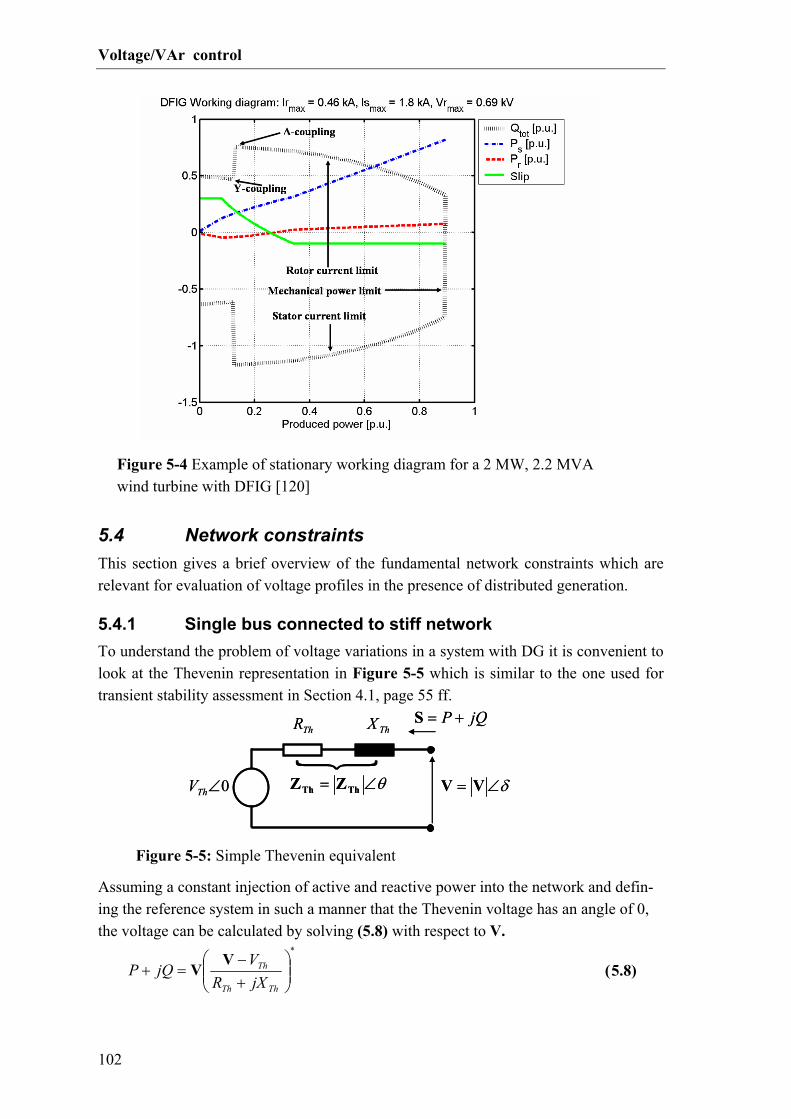
Voltage/VAr control
102
5.4 Network constraints This section gives a brief overview of the fundamental network constraints which are relevant for evaluation of voltage profiles in the presence of distributed generation.
5.4.1 Single bus connected to stiff network To understand the problem of voltage variations in a system with DG it is convenient to look at the Thevenin representation in Figure 5-5 which is similar to the one used for transient stability assessment in Section 4.1, page 55 ff.
Assuming a constant injection of active and reactive power into the network and defin-ing the reference system in such a manner that the Thevenin voltage has an angle of 0, the voltage can be calculated by solving (5.8) with respect to V.
*
+−
=+ThTh
Th
jXRV
jQPV
V ( 5.8)
Figure 5-4 Example of stationary working diagram for a 2 MW, 2.2 MVA wind turbine with DFIG [120]
ThXThR
δ∠= VV0∠ThV
jQP +=S
θ∠= ThTh ZZ
ThXThR
δ∠= VV0∠ThV
jQP +=S
θ∠= ThTh ZZ
Figure 5-5: Simple Thevenin equivalent

Voltage/VAr control
103
This gives a complex quadratic equation. The solution in the form of (5.9) was formu-lated in [29]. Because of the quadratic nature of (5.8), it has two solutions for combina-tions of P and Q which are physically possible. Only the solution where Q∂∂ /V in
(5.12) is positive denotes a stable operation point with a constant P and Q injection [71].
( )Th
ThThThTh
Th
ThThThTh V
QRPXjQXPR
VQRPX
VV−
+
+−
−−±=
22 4
21V ( 5.9)
The sensitivity of the voltage to a small change in active or reactive power injection can be derived by differentiating (5.9) with respect to P or Q as shown in (5.10) and (5.11).
( )
( )Th
Th
ThThTh
ThThTh
Th
ThThThTh
VX
j
QXPRV
QRPXV
VXRQXP
R
P+
+−
−−
⋅−⋅−
±=∂∂
22
2
4
2V ( 5.10)
( )
( )Th
Th
ThThTh
ThThTh
Th
ThThThTh
VR
j
QXPRV
QRPXV
VRRQXP
X
Q−
+−
−−
⋅−⋅+
±=∂∂
22
2
4
2V ( 5.11)
The sensitivity of the voltage magnitude is only affected by the part which is parallel to V, which is expressed in (5.12).
⋅ℜ=
∂
∂
VVVV *
dPd
P and
⋅ℜ=
∂
∂
VVVV *
dQd
Q ( 5.12)
When the injection of active and reactive power is low compared to the short circuit power, the voltage at the connection point can be approximated with the first order Tay-lor expansion in (5.13) by setting P and Q in (5.10) and (5.11) to zero.
th
ThTh
th
ThThthQP V
QRPXj
VQXPR
V−
++
+≈≈≈ 0,0
V ( 5.13)
Figure 5-6 A shows the P/V curves of a connection point with a Thevenin voltage of 1 p.u., an X/R ratio of 3 and different sort circuit ratios (SCR). The SCR is defined as the short circuit power over the power base of the per unit conversion. These curves are also denoted “nose curves” in most books dealing with power system operation due to their shape. For small injections of active power, the voltage magnitude is increased because of the voltage drop over the resistive part of the impedance. For larger injections, the voltage magnitude decreases because of the voltage drop over the reactive part of the impedance. One thing which is worth noticing, is that all the curves corresponding to a given X/R ratio and a given Thevenin voltage have the same shape, but their X-axes are stretched proportionally to the short circuit ratio. This means that the maximal voltage and the voltage at the point where the system becomes marginally stable are independ-

Voltage/VAr control
104
ent of the short circuit ratio. One way to explain this is that if the resistance and the re-actance in (5.9) are multiplied with a common factor, and the active and reactive power are multiplied with the reciprocal factor, the result is unchanged. Figure 5-6 C shows the angle of the voltage in the same situations. Because the voltage magnitude at the connection point is not maintained at a constant magnitude, the insta-bility occurs before the angle is 90°, when no reactive power is injected.
In cases where there is a well defined relation between the active and the reactive power injection at a connection point, for example in case of a no-load compensated Danish concept wind turbine or a CHP operating with a constant power factor, the sensitivity of the voltage to a change in active power injection including the resulting change in reac-tive power injection can be calculated using the chain rule as defined in (5.14).
( ) P
QQPdP
d
PfQ∂∂
∂
∂+
∂
∂=
=
VVV ( 5.14)
For a no load compensated Danish concept wind turbine, the reactive power consump-tion is approximately proportional to the square of the active power production. This
X/R = 3, Q = 0A B
C D
X/R = 3, Q = 0A B
C D
X/R = 3, Q = 0A B
C D
Figure 5-6: Voltage profiles for networks with different short circuit ratios.

Voltage/VAr control
105
can be formulated as (5.5), page 99. Inserting (5.5) in (5.14) gives the resulting voltage sensitivity in (5.15) where the weighting of the two partial derivatives is dependent on the per unit production.
QPP
kPdP
d
ratedwind
windQ
comploadno∂
∂−
∂
∂≈
−−−
VVV2 ( 5.15)
In case of a CHP which is operated with a constant power factor, the resulting sensitiv-ity can be expressed as (5.16) where the weighting of the partial sensitivities is inde-pendent on the active power production.
( )
( )QPdP
d
PQ∂
∂+
∂
∂=
=
VVVφ
φ
tantan
( 5.16)
5.4.1.1 Voltage rise As described for example in [23;24;121;122], a common problem when connecting a generator to a distribution system through a long power line with a low X/R – ratio it voltage rise. It was shown in Figure 5-6 A that the maximal voltage rise at a power fac-tor of 1 is not dependent on the short circuit ratio at the connection point but only on the X/R – ratio and the Thevenin voltage. In this section, a heuristically derived approxima-tion of the maximal voltage rise is presented. The magnitude of the voltage in (5.9) can be found using (5.17).
*VVV ⋅= ( 5.17)
The voltage can be approximated using the second order Taylor approximation about P=0 in (5.18). The strict second order Taylor expansion also contains the term
232 / PVR Th , but comparing the Taylor expansion with the output from (5.9) and (5.17)
shows that a better fit in the area of interest is achieved by omitting the resistance in the second order term. The reason is that the coefficients of the higher order terms in the Taylor expansion do not converge to zero.
23
2
2P
VXP
VR
VThTh
ThTh −+≈V ( 5.18)
Figure 5-7 shows the voltage profiles with different X/R – ratios together with the first and second order approximations according to (5.18). At high X/R ratios, the first order approximation is only valid for very low power injections, where as the second order approximation provides a very good estimate of the voltage rise. When the X/R ratio is below 1.5, the second order term has only little effect in the area where the voltage is within acceptable limits. The maximal voltage rise is therefore not relevant there.

Voltage/VAr control
106
The maximal voltage at injection of only active power can be estimated with the maxi-mum of the quadratic approximation. With the approximation in (5.19), the relative voltage rise is proportional to the square of the R/X ratio and independent on the The-venin voltage and the short circuit power.
+≈
2
211
Th
ThTh X
RVmaxV ( 5.19)
In Figure 5-7 C where the X/R ratio is 2.3, the exactly calculated voltage change is 9.04 %, and the estimated voltage rise using (5.18) is 9.45 %. This is a deviation of 4.5 % which is considered a good accuracy considering the variation in the parameters which are usually available for such calculations. The power injection where the maximal voltage rise occurs can be approximated with (5.20). As described earlier, the power at which the maximal voltage occurs is directly proportional to the short circuit power.
( )2
2
cos ThSC
Th
Th
Th
Th
Th
ThVmax
VS
XR
XV
XR
Pθ
=≈ ( 5.20)
SCR = 5, Q = 0SCR = 5, Q = 0
Figure 5-7: Voltage profiles for different X/R ratios compared to the first and second order approximations of (5.18)

Voltage/VAr control
107
When considering a connection point for a distributed generation unit, (5.19) and (5.20) can be used for a rough estimate of the expected problems with voltage rise. If the X/R ratio is over 3, (5.19) states that the maximally occurring voltage rise is below 6 %. If the point where the maximal voltage occurs in (5.20) is much higher than the rated po-wer of the generator, it can be considered reasonable to use the linear approximation to calculate the maximally occurring voltage rise. If the voltage at a given point is controlled with an automatic tap changer, the Thevenin voltage should be set to the upper limit of the control band, and the Thevenin impedance should only include the part of the network from the connection point to the bus with the voltage control. An example of this is given in Section 6.7.2, page 145. Consumers, located at the same radial as the generator, will contribute to keeping the voltage down. A conservative method is to insert the estimated minimal load at the point of common coupling and calculate the maximal voltage rise based on the rated power production in this situation. Alternatively, a higher load can be assumed, which enables the installation of more generation. In the relatively short periods where the potential maximal production would lead to too high a voltage, the production can be curtailed. A method for optimizing the operation of tap changers, reactive power com-pensation and generator curtailment, with respect to economical costs is presented in [25]. For a CHP, a short curtailment period is usually not critical because the fuel can be saved for later, and the heat demand can often be met by the reservoir tanks. Further, the CHP will tend to operate in periods where the load demand is high and the prices are high. For a wind farm, on the other hand, a curtailment means that the potential energy is spilled.
5.4.1.2 Limits for reactive power injection As mentioned earlier, voltage control is usually not performed by generators in MV and LV networks. However, distributed generators are often used to provide or absorb reac-tive power, for example, time dependent power factor control is in some cases used to make the CHPs compensate for the reactive power absorption of the consumers. Alter-natively, a generator connected at the end of a long radial could absorb reactive power in low load periods to limit the voltage rise effect. This section briefly describes how the voltage magnitude constraints the reactive power transfer at a given connection point. The constraints imposed by the upper and lower voltage magnitude limit are assessed the same way as the reactive power capability for the DFIG in [120]. The approach is to calculate the active and reactive power injection when the voltage at the connection point is set to a fixed magnitude corresponding to the upper or lower limit and a varying angle. Equation (5.21) shows how the power injection can be calculated from the The-venin voltage, the voltage at the connection point and the Thevenin impedance. The last expression shows that if the angle of the voltage at the connection point is varied be-tween 0 and 360°, the apparent power will form a circle in the complex plane with a

Voltage/VAr control
108
center corresponding to the first term and a radius corresponding to the magnitude of the second term.
( )θδ +⋅⋅
−=
−⋅= jThTh e
VV
ThThTh ZV
ZV
ZV
VS *
2*
( 5.21)
Figure 5-8 B shows the Q/P curves for three different voltage magnitudes and one for a constant current when the voltage is 1 p.u. The curves corresponding to 0.95 and1.05 p.u. denote the lower and upper limits of reactive power which can be injected, given the latter voltage limits. Further, the generator imposes limits for the reactive power exchange, for example the current magnitude must be below the rated current. A gen-erator with a rated power of 1 p.u. connected to the given network can at its rated power production inject approximately 0.3 p.u. of reactive power before the voltage exceeds 1.05 p.u.. Figure 5-8 A visualizes the geometric interpretation of (5.21). It can be seen, how the center and radius of the circles change with changing parameters. The follow-ing empiric observations can be made:
• The circles where the Thevenin voltage and the voltage magnitude at the con-nection point are the same always go through P,Q = 0,0
• If the Thevenin voltage is raised, only the radius is affected – this means that the lower rims of the circles are lowered. This means that less reactive power can be supplied and more reactive power can be absorbed at given voltage limits.
• If the X/R ratio is decreased, the circles will tilt to the right which will give stee-per curves in the normal operation area depicted in Figure 5-8 B. This means that at higher active power productions, reactive power may have to be absorbed to keep the voltage below the upper limit.
• If the short circuit ratio is decreased (the magnitude of the per unit Thevenin im-pedance is increased), the radius of the circles becomes smaller, and the center moves closer to the origin. This means that the curvature in plot B becomes lar-ger. Further, the curves corresponding to the upper and lower voltage limit move closer to each other which makes the control interval smaller.
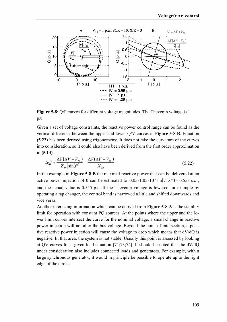
Voltage/VAr control
109
Given a set of voltage constraints, the reactive power control range can be found as the vertical difference between the upper and lower Q/V curves in Figure 5-8 B. Equation (5.22) has been derived using trigonometry. It does not take the curvature of the curves into consideration, so it could also have been derived from the first order approximation in (5.13).
( )
( )( )
Th
Th
Th
Th
XVVV
ZVVV
Q+∆∆
=+∆∆
≈∆θsin
( 5.22)
In the example in Figure 5-8 B the maximal reactive power that can be delivered at an active power injection of 0 can be estimated to ( ) .. 553.06.71sin/1005.105.0 up=°⋅⋅ , and the actual value is 0.555 p.u. If the Thevenin voltage is lowered for example by operating a tap changer, the control band is narrowed a little and shifted downwards and vice versa. Another interesting information which can be derived from Figure 5-8 A is the stability limit for operation with constant PQ sources. At the points where the upper and the lo-wer limit curves intersect the curve for the nominal voltage, a small change in reactive power injection will not alter the bus voltage. Beyond the point of intersection, a posi-tive reactive power injection will cause the voltage to drop which means that dV/dQ is negative. In that area, the system is not stable. Usually this point is assessed by looking at QV curves for a given load situation [71;73;74]. It should be noted that the dV/dQ under consideration also includes connected loads and generators. For example, with a large synchronous generator, it would in principle be possible to operate up to the right edge of the circles.
*
2
ThZV ThZ
V ThV⋅
Stability limit
VTh = 1 p.u., SCR = 10, X/R = 3A B
θ
( )ThZ
ThVVV +∆∆
ThVV +∆=V
*
2
ThZV ThZ
V ThV⋅
Stability limit
VTh = 1 p.u., SCR = 10, X/R = 3A B
θ
( )ThZ
ThVVV +∆∆
ThVV +∆=V
*
2
ThZV ThZ
V ThV⋅
Stability limit
VTh = 1 p.u., SCR = 10, X/R = 3A B
θ
( )ThZ
ThVVV +∆∆
ThVV +∆=V
Figure 5-8: Q/P curves for different voltage magnitudes. The Thevenin voltage is 1 p.u.
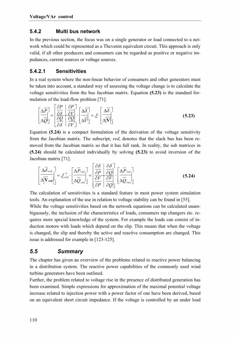
Voltage/VAr control
110
5.4.2 Multi bus network In the previous section, the focus was on a single generator or load connected to a net-work which could be represented as a Thevenin equivalent circuit. This approach is only valid, if all other producers and consumers can be regarded as positive or negative im-pedances, current sources or voltage sources.
5.4.2.1 Sensitivities In a real system where the non-linear behavior of consumers and other generators must be taken into account, a standard way of assessing the voltage change is to calculate the voltage sensitivities from the bus Jacobian matrix. Equation (5.23) is the standard for-mulation of the load-flow problem [71].
∆
∆⋅=
∆
∆⋅
∂∂
∂∂
∂∂
∂∂
=
∆
∆
V
δδ
δ
δ JV
VQQVPP
Q
P ( 5.23)
Equation (5.24) is a compact formulation of the derivation of the voltage sensitivity from the Jacobian matrix. The subscript, red, denotes that the slack bus has been re-moved from the Jacobian matrix so that it has full rank. In reality, the sub matrices in (5.24) should be calculated individually by solving (5.23) to avoid inversion of the Jacobian matrix [71].
∆
∆⋅
∂∂
∂∂
∂∂
∂∂
=
∆
∆⋅=
∆
∆−
red
red
red
red
red
red
Q
P
QV
PV
QPQ
PJ
δδδ
1
redV ( 5.24)
The calculation of sensitivities is a standard feature in most power system simulation tools. An explanation of the use in relation to voltage stability can be found in [55]. While the voltage sensitivities based on the network equations can be calculated unam-biguously, the inclusion of the characteristics of loads, consumers tap changers etc. re-quires more special knowledge of the system. For example the loads can consist of in-duction motors with loads which depend on the slip. This means that when the voltage is changed, the slip and thereby the active and reactive consumption are changed. This issue is addressed for example in [123-125].
5.5 Summary The chapter has given an overview of the problems related to reactive power balancing in a distribution system. The reactive power capabilities of the commonly used wind turbine generators have been outlined. Further, the problem related to voltage rise in the presence of distributed generation has been examined. Simple expressions for approximation of the maximal potential voltage increase related to injection power with a power factor of one have been derived, based on an equivalent short circuit impedance. If the voltage is controlled by an under load

Voltage/VAr control
111
tap changing transformer, the equivalent short circuit impedance for calculation of the voltage rise effect is the impedance between the connection point under consideration and the bus where the voltage is controlled. It is concluded that voltage rise only consti-tutes a problem, when the X/R ratio of the equivalent short circuit impedance is below 3. The limit for reactive power transfer, imposed by the upper and lower voltage magni-tude limits have been visualized by plotting the P/Q curves corresponding to the upper and lower voltage magnitude limits in the complex plane. This makes it possible to stu-dy the effect of changing the Thevenin voltage, the short circuit capacity, the X/R ratio and the limits of the voltage magnitude in a geometric way.

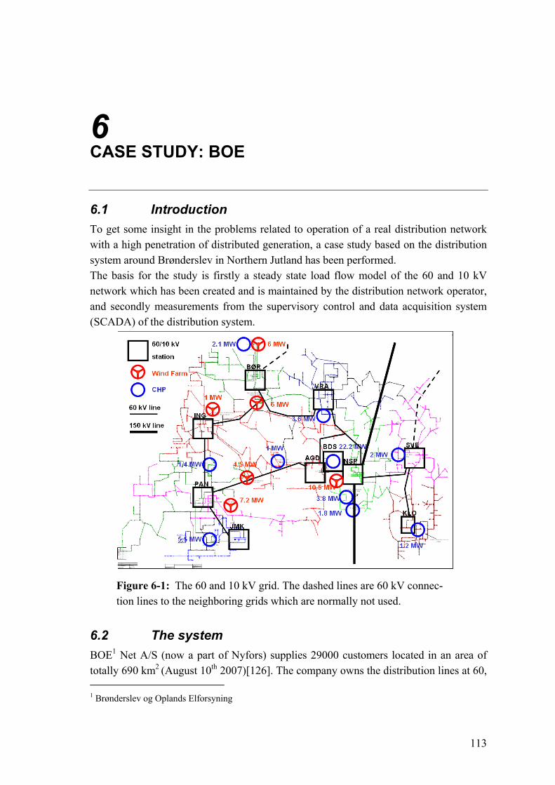
113
6 CASE STUDY: BOE
6.1 Introduction To get some insight in the problems related to operation of a real distribution network with a high penetration of distributed generation, a case study based on the distribution system around Brønderslev in Northern Jutland has been performed. The basis for the study is firstly a steady state load flow model of the 60 and 10 kV network which has been created and is maintained by the distribution network operator, and secondly measurements from the supervisory control and data acquisition system (SCADA) of the distribution system.
6.2 The system BOE1 Net A/S (now a part of Nyfors) supplies 29000 customers located in an area of totally 690 km2 (August 10th 2007)[126]. The company owns the distribution lines at 60, 1 Brønderslev og Oplands Elforsyning
Figure 6-1: The 60 and 10 kV grid. The dashed lines are 60 kV connec-tion lines to the neighboring grids which are normally not used.

Case study: BOE
114
10 and 0.4 kV levels. The grid is only connected to the transmission system through the 150/60 kV station in Nibstrup (NSP) east of Brønderslev (BDS), but it can be connected to the neighboring system through two 60 kV lines. There are ten 60/10 kV transformer stations and 727 10/0.4 kV stations. The 10 kV system consists of approximately 615 km cables and 130 km overhead lines, and the 60 kV system comprises 10 km cables and 110 km overhead lines. In this investigation, the 0.4 kV system is not modeled, but considered a part of the loads. A sketch of the 60 and 10 kV grid including the major
production units and the 150 kV infeed is shown in Figure 6-1. The 60 kV network is partly operated as a meshed system, and the 10 kV network is operated as radials. The larger wind farms and CHPs have their own 10 kV radial, and the smaller units are connected together with the consumers at the 10 kV level. The load varies between 15 and 45 MW. Approximately 65 wind turbines with a total rated power of 38.5 MW and 20 combined heat and power plants with a total rated power of 50 MW are connected to the system. The short circuit power at the connection to the 150 kV transmission system is ap-proximately 2500 MVA when both 150 kV lines are in service.
Figure 6-2: Principal structure of the system. The grey boxes indicate measurements

Case study: BOE
115
6.2.1 Measurements The system is equipped with an energy measurement system and an online sampling system. Figure 6-2 shows a principal overview of the measurements which were used in the investigation.
6.2.1.1 Energy measurements for billing The Danish transmission system operator (TSO) Energinet.dk is responsible for selling the energy from most wind turbines and small CHPs in the country on the Nord Pool electricity exchange and for paying subsidies to them according to their delivered en-ergy. Therefore, every production unit has an energy measurement system which meas-ures the produced energy during each 15 min period. The measurements are stored lo-cally in the units and gathered with modem connections by the distribution network operator (DNO) and sent to the TSO once a day. Further, the 150/60 kV transformer station has measurements of active and reactive energy.
6.2.1.2 Online measurements for remote control and diagnosis Online measurements are gathered with the SCADA system, BECOS 32®, from ABB®. Every 5 minutes, an instant value of the quantities shown in Figure 6-2 (Plus some currents which are not used in the investigation) are captured. There is no exact time stamp on the measurements. It is therefore not guarantied that they are concurrent. When the communication with the measurement system is interrupted due to faults in the communication system, the data is lost. For the investigation, the relevant measure-ments have been included in the data stream which is logged in the control room of En-erginet.dk. The extra measurements have been logged since April 6th 2006, and the last data extraction for the project was made on February 6th 2007. This gives 10 months of data.
6.3 Simulation of the system A complete steady state model of the 60 and 10 kV system including the components shown in Figure 6-2 is maintained in the power system simulation tool, Neplan® by BOE-Net A/S. The Neplan model corresponds to the state of the network on April 24th, 2005. The only change in the model since that point in time is the inclusion of the 10.5 MW wind farm in Ryå. This means that the actual location of the consumers and cou-pling of the 10 kV radials may differ from the model in the later simulations. For the purpose of this investigation, the model has been converted to the power system simulation tool PowerFactory® from DIgSILENT®. Figure 6-1 shows the 10 kV sys-tem excluding the city of Brønderslev. To be able to estimate the load and the active and reactive losses in the system, a series of load flow calculations has been carried out with 15 min time steps. For compliance with the energy measurements, the online 5 min measurements have been used to esti-

Case study: BOE
116
mate 15 min mean values which have been used as basis for the simulation. The period contains a total of approximately 27000 simulation steps.
6.3.1 Modeling of the components
6.3.1.1 Transformers The 150/60 and 60/10 kV transformers are equipped with automatic tap changers. For the 150/60 kV transformers, the tap positions are measured online. The tap position has to be an integer value in PowerFactory®, it is therefore not possible to insert the mean value during the interval. Instead, the tap position is set to the value it had just at the beginning of the interval under consideration. For the 60/10 transformers, the voltage set point on the secondary side is known, and the tap-position is estimated by Power-Factory®. The measured voltage at the 150 kV side of the 150/60 kV transformers is inserted as voltage for the external grid. The voltage at the 60 kV side is used for comparison be-tween measured and simulated data.
6.3.1.2 CHPs The large CHPs have online measurements of active and reactive power. The synchro-nous machines have been implemented as PQ–sources delivering the measured active and reactive power. For the CHPs with only energy measurements, a tan(φ) of 0.4 has been assumed, since this is the requirement from BOE Net A/S. These CHPs only have a total rated power of 4.8 MW. It has been verified that the reactive power of the loads in a given feeder which is estimated as shown in Figure 6-3 does not make a jump when a CHP connected to the feeder cuts in or out.
6.3.1.3 Wind turbines All the wind turbines in the system use the “Danish Concept”. This means that have an induction generator which is connected directly to the grid and reactive power compen-sation with fixed and in some cases switchable shunt capacitors. Wind turbines con-nected before 1998 are only obliged to install shunt capacitors corresponding to the no-load consumption of the generators. In 1998 it was specified in [75] that the load de-pendent reactive power consumption must be compensated - e.g. with switchable ca-pacitors. In 2004 the requirements were extended to also include the reactive losses in the wind turbine transformer [15]. In the area, wind turbines with a rated power of totally 16.5 MW are full load compen-sated and the remaining turbines with a rated power of 22 MW are no-load compen-sated. Most of the no load compensated wind turbines have been installed after 1998, but an agreement has been made with BOE Net A/S to perform the reactive power com-pensation centrally.
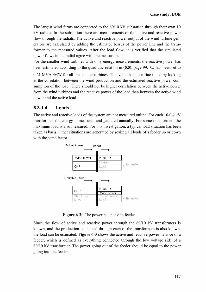
Case study: BOE
117
The largest wind farms are connected to the 60/10 kV substation through their own 10 kV radials. In the substation there are measurements of the active and reactive power flow through the radials. The active and reactive power output of the wind turbine gen-erators are calculated by adding the estimated losses of the power line and the trans-former to the measured values. After the load flow, it is verified that the simulated power flows in the radial agree with the measurements. For the smaller wind turbines with only energy measurements, the reactive power has been estimated according to the quadratic relation in (5.5), page 99. Qk has been set to
0.21 MVAr/MW for all the smaller turbines. This value has been fine tuned by looking at the correlation between the wind production and the estimated reactive power con-sumption of the load. There should not be higher correlation between the active power from the wind turbines and the reactive power of the load than between the active wind power and the active load.
6.3.1.4 Loads The active and reactive loads of the system are not measured online. For each 10/0.4 kV transformer, the energy is measured and gathered annually. For some transformers the maximum load is also measured. For this investigation, a typical load situation has been taken as basis. Other situations are generated by scaling all loads of a feeder up or down with the same factor.
Since the flow of active and reactive power through the 60/10 kV transformers is known, and the production connected through each of the transformers is also known, the load can be estimated. Figure 6-3 shows the active and reactive power balance of a feeder, which is defined as everything connected through the low voltage side of a 60/10 kV transformer. The power going out of the feeder should be equal to the power going into the feeder.
Figure 6-3: The power balance of a feeder
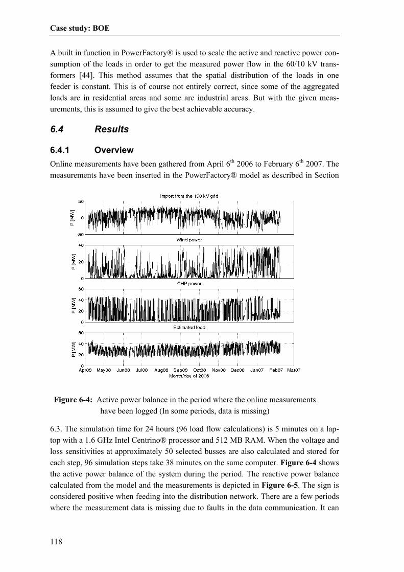
Case study: BOE
118
A built in function in PowerFactory® is used to scale the active and reactive power con-sumption of the loads in order to get the measured power flow in the 60/10 kV trans-formers [44]. This method assumes that the spatial distribution of the loads in one feeder is constant. This is of course not entirely correct, since some of the aggregated loads are in residential areas and some are industrial areas. But with the given meas-urements, this is assumed to give the best achievable accuracy.
6.4 Results
6.4.1 Overview Online measurements have been gathered from April 6th 2006 to February 6th 2007. The measurements have been inserted in the PowerFactory® model as described in Section
6.3. The simulation time for 24 hours (96 load flow calculations) is 5 minutes on a lap-top with a 1.6 GHz Intel Centrino® processor and 512 MB RAM. When the voltage and loss sensitivities at approximately 50 selected busses are also calculated and stored for each step, 96 simulation steps take 38 minutes on the same computer. Figure 6-4 shows the active power balance of the system during the period. The reactive power balance calculated from the model and the measurements is depicted in Figure 6-5. The sign is considered positive when feeding into the distribution network. There are a few periods where the measurement data is missing due to faults in the data communication. It can
Figure 6-4: Active power balance in the period where the online measurements have been logged (In some periods, data is missing)
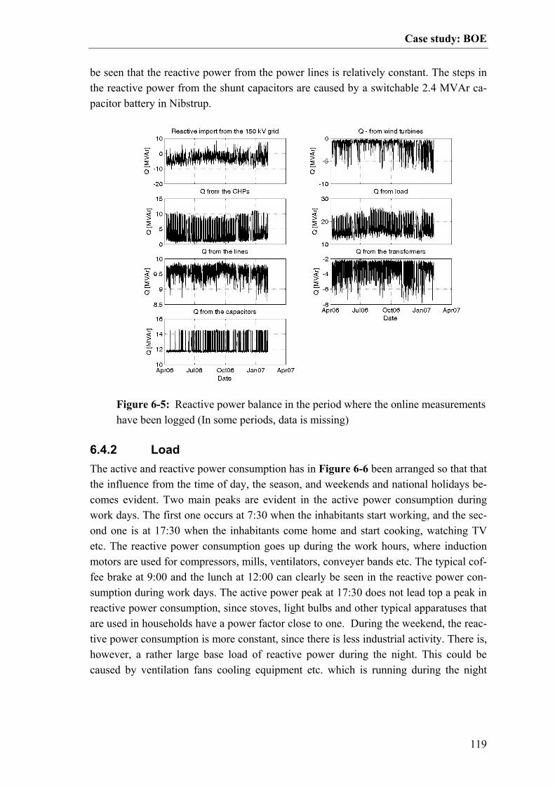
Case study: BOE
119
be seen that the reactive power from the power lines is relatively constant. The steps in the reactive power from the shunt capacitors are caused by a switchable 2.4 MVAr ca-pacitor battery in Nibstrup.
6.4.2 Load The active and reactive power consumption has in Figure 6-6 been arranged so that that the influence from the time of day, the season, and weekends and national holidays be-comes evident. Two main peaks are evident in the active power consumption during work days. The first one occurs at 7:30 when the inhabitants start working, and the sec-ond one is at 17:30 when the inhabitants come home and start cooking, watching TV etc. The reactive power consumption goes up during the work hours, where induction motors are used for compressors, mills, ventilators, conveyer bands etc. The typical cof-fee brake at 9:00 and the lunch at 12:00 can clearly be seen in the reactive power con-sumption during work days. The active power peak at 17:30 does not lead top a peak in reactive power consumption, since stoves, light bulbs and other typical apparatuses that are used in households have a power factor close to one. During the weekend, the reac-tive power consumption is more constant, since there is less industrial activity. There is, however, a rather large base load of reactive power during the night. This could be caused by ventilation fans cooling equipment etc. which is running during the night
Figure 6-5: Reactive power balance in the period where the online measurements have been logged (In some periods, data is missing)

Case study: BOE
120
also. The major seasonal deviation can be seen in the active power consumption during the winter. It should be noted that data from February and March is missing, which affects the
mean values in the winter and spring.
6.4.3 CHPs The active and reactive production from the CHPs in the area, arranged in the same manner as the loads, is depicted in Figure 6-7. The primary objective of the CHPs is to meet the heat demand of the costumers, and the secondary objective is to sell the elec-trical power with as much profit as possible. The thermal energy can be stored in large accumulator tanks which makes it possible to operate the machines when the electrical energy prices are highest and to operate the generators only at full load for better effi-ciency. As seen in Figure 6-7, the CHPs are usually started at 7:00 at work days, and they are operated for as long as it takes to store enough thermal energy to meet the de-
Figure 6-6: The active and reactive power of the loads. The curves represent the mean values of each 15 minute period. The seasons are defined as follows: winter: December-February, spring: March-May, summer: June-August and au-tumn: September – November. Notice that data from February and March is missing.

Case study: BOE
121
mand during the night. Therefore, the CHPs stay connected for a longer period during the winter than during the summer. The mean production around noon is lower in the winter than in the other seasons in the period under consideration. The reason is that some generators for some reason have not been operated in this period. In the weekends, where the electricity prices are usually lower than in the work days, the production from the CHPs is lower. A part of the explanation could be that the heat demand can be met by the heat capacity in the storage tanks. Another reason could be that heat demand of
some industrial consumers is lower during the weekend. Before 2005, most Danish CHPs have been paid according to the three step tariff where different fixed power prices are paid in low load, high load and peak load periods. Ac-cording to the Law 495 [127], all production units with a rated power above 10 MW must be paid according to spot market prices after 2005, and after 2007 this must also apply for plants between 5 and 10 MW. It has not been investigated how the CHPs in the area are paid, but in the future it is possible that the CHPs start acting more directly
Figure 6-7: The active and reactive power of the CHPs. The curves represent the mean values of each 15 minute period. The seasons are defined as follows: winter: December-February, spring: March-May, summer: June-August and au-tumn: September – November. Notice that data from February and March is missing.

Case study: BOE
122
to spot market prices. This could for example mean that many CHPs would shut down in periods with high wind power production.
6.4.4 Wind power The peak wind production in the area is close to 40 MW. Figure 6-8 A shows duration curves for the wind power production in the time interval under consideration. There is a clearly higher production during the winter than during the summer. The curve for the spring and the autumn are close to the average of the whole period. The relation be-tween the active power production and the reactive power consumption of the genera-tors can be seen in Figure 6-8 B.
Based on a linear regression, the total consumption of the generators minus the compen-sation capacitors can be approximated with (6.1), and the reactive power consumption of the step up transformers can be estimated with (6.2).
MW
PMVArQ wind
fitgenWind 5.3813.025.0
2
+=−− ( 6.1)
MW
PMVArQ wind
fittrafoWind 5.38042.044.0
2
+=−− ( 6.2)
6.4.5 Active and reactive power exchange with the transmis-sion system Figure 6-7 shows the active and reactive power import from the 150 kV transmission system on the 60 kV side of the transmission transformers. The variation of the mean exchange over the day is smaller than the variation in the mean load and mean CHP production because the time profile of the CHPs partly compensates for the time de-pendent variation of the load. For the reactive power, it can be seen that there is a mean export, especially during the night.
A BA B
Figure 6-8: A: duration curves for the total wind production. B: relation between the total active power production and the total reactive power absorption of the generators minus the reactive power compensation. The solid curve denotes a least square quadratic fit.
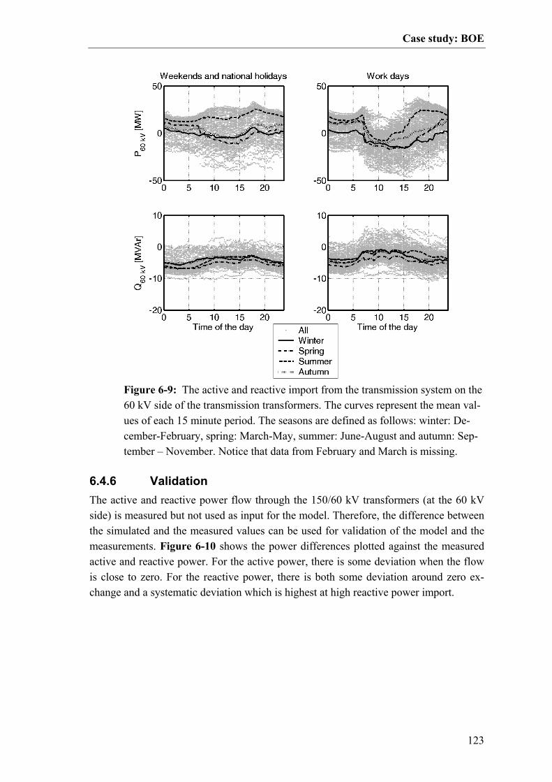
Case study: BOE
123
6.4.6 Validation The active and reactive power flow through the 150/60 kV transformers (at the 60 kV side) is measured but not used as input for the model. Therefore, the difference between the simulated and the measured values can be used for validation of the model and the measurements. Figure 6-10 shows the power differences plotted against the measured active and reactive power. For the active power, there is some deviation when the flow is close to zero. For the reactive power, there is both some deviation around zero ex-change and a systematic deviation which is highest at high reactive power import.
Figure 6-9: The active and reactive import from the transmission system on the 60 kV side of the transmission transformers. The curves represent the mean val-ues of each 15 minute period. The seasons are defined as follows: winter: De-cember-February, spring: March-May, summer: June-August and autumn: Sep-tember – November. Notice that data from February and March is missing.

Case study: BOE
124
The active and reactive power flows have been plotted as duration curves in Figure 6-11. There seems to be a dead band around zero exchange both for the measured active and the reactive power flow.
The rated power of each of the transformers is 100 MVA so the deviations are relatively small in that context, but compared to the size of the allowable MVAr band of -9 to 2, MVAr [128], the deviations are relatively large. The simulations are, based on power measurements at the low voltage side of fifteen 60/10 kV transformers. Deviations in the simulated power flows can therefore only be caused by faults in these measurements or faults in the modeling of the 60/10 kV transformers or the 60 kV lines. It is assumed that some of the measurement uncertainties of the 60/10 kV transformers will cancel
Figure 6-10: Difference between the measured and simulated power flow on the 60 kV side of the 150/60 kV transformer. The measured values are used for the x-axes, and the solid curves denote mean values, based on 100 equidistant bins on the x-axis.
Figure 6-11: Duration curves measured and simulated power flow on the 60 kV side of the 150/60 kV transformer. The flow is considered positive from 150 kV to 60 kV

Case study: BOE
125
each other out. If possible, a validation and eventually a calibration of the measurement equipment should be made before investments are made based on the simulations. The voltage of the transmission system which has been used for the simulation has been calculated as the mean value of two measurements in the transformer station. The two measurements and the mean value that have been used for the simulation are depicted in Figure 6-12 A. Figure 6-12 B shows the voltage measurements of the two transformers together with the simulated voltage. Since the measured 60 kV voltages have not been used as input for the simulation, they can be used for validation of the simulation re-sults. The simulated voltage lies between the two measured voltages most of the time which indicates that the modeling of the transformer is correct. Changes in the tap posi-tion in Figure 6-12 C do not lead to larger deviations in the voltage, although the changes occur within a 15 minute period, and the simulation assumes a constant tap setting during the entire interval.
Figure 6-12: The simulated and measured voltages of the 150/60 kV transformer station

Case study: BOE
126
The active and reactive load is in principle estimated from the remaining space in
Figure 6-3. If for example the reactive power consumption of the wind turbines under a given 60/10 kV transformer is underestimated, the reactive consumption of the loads will be overestimated in order to fill the gap and vice versa. Therefore, the correlation between the reactive load and the wind production should not be significantly larger than the correlation between the active load and the wind production. Figure 6-13 shows the active and reactive load plotted against the wind production. The dark curves show a least square second order fit. The trend is that both the reactive and the active power of the loads are slightly lower at low output from the wind turbines than at me-dium and high output. This could be due to the fact that both the wind production and the load are lower in the night than in the day and lower in the summer than in the win-ter. The trend curve for the reactive power does not imply a large systematic deviation in the estimation of the reactive power consumption from the wind turbines.
6.5 Analysis of the losses The active and reactive power losses of the system have been analyzed according to the methods described in Chapter 3. The aim of the analysis is twofold. Firstly, it is supposed to provide an overview of the losses in the distribution system. The following questions should be considered:
1. How large are the total losses compared to the load and production? 2. Where in the system do most of the losses occur?
a. Which feeders? b. Which components?
3. What are the losses caused by the integration of DG?
Figure 6-13: The correlation between wind and load. The dark curves show a second order least square fit

Case study: BOE
127
4. What are the losses caused by the transfer of reactive power? 5. What are the potential savings in losses if the simultaneity between load and
production is increased? Secondly, the analysis will serve as a validation of the loss allocation methods presented in Chapter 3. The analyses are based on measurements obtained in the period April 6th 2006 to Febru-ary 6th 2007. During the period a few days of data are missing due to communication problems in the SCADA system. The estimated mean values of losses etc. have not been corrected for the difference in load and production pattern between the missing two months and the rest of the year. Figure 6-14 shows an overview of the mean active power losses, divided into the com-ponents causing the losses. The total mean-losses make approximately 1.27 MW, from which 72 % is dissipated at 10 kV level and below. It should be noted that the real sys-tem also comprises a large number of 0.4 kV lines which have not been modeled. The shunt losses of the transformers which are practically independent of the loading, make 49 % of the total active power losses. The mean load dependent losses of the 150/60 kV transformers only amount to 5 kW. For the reactive power losses, the concern is not to minimize the mean losses, but to
Figure 6-14: Mean active power losses

Case study: BOE
128
maintain a reactive power balance at all times. Figure 6-15 shows the reactive sinks and sources of the system. It can be seen that the reactive power losses are relatively small compared to the reactive power consumption of the loads. A thorough explanation of the reactive power balance can be found in [61]
6.5.1 Allocation of losses To study the impact of the distributed generation, an allocation of the system losses is performed as described in Section 3.2 and 3.3, page 34 ff. Since the BOE system is much larger than the small example which was treated in section 3.2.3 and section 3.3.4, it wouldn’t be feasible to analyze it in exactly the same way. Instead, the following combination of the methods has been used: Firstly the losses of the 60 kV network, the 150 / 60 kV transformers and the 60 / 10 kV transformers are allocated to the individual feeders, based on the impedance matrix of that part of the network. For comparison, the allocation is made both using the marginal loss allocation method described in section 3.2.1 page 35 and the statistical method based on current injections, described in section 3.3.2 page 45. Secondly, the losses at 10 kV level and below for each feeder are allocated to the four categories; loads, wind turbines, CHPs and shunt losses. The allocation is performed
Figure 6-15: Mean reactive power balance of the system. The reactive power consumption of the wind turbines includes the losses in the step up transformers

Case study: BOE
129
using the regression method, described in section 3.3.1 page 43 using the apparent po-wer as input and neglecting the cross effects. Finally, the losses at 60 kV and above are allocated to the loads, wind turbines, CHPs and shunt losses of the individual feeders. The approach is that the load or generation of each category minus the low voltage losses allocated to the specific category are con-verted to an equivalent current injection on the 10 kV side of the 60 / 10 kV transform-ers, and the same approach as in step one is used.
6.5.1.1 Allocation of 60 kV losses to the individual feeders The basis for this analysis is a model of the 60 kV network including the 150/60 kV transformers and the 60/10 kV transformers. The reduced impedance matrix, IZ , calcu-
lated according to (3.8) page 32, is shown in Appendix C, page 181. The network pa-rameters were obtained by printing the transformer and line parameters with a DPL script in PowerFactory®, and importing them into Matlab®. The tap changers of the transformers have been set to their average value during the period of measurements Based on the full impedance matrix and the measured power flows through the low vol-tage side of the 60/10 kV transformers, a series of load flow calculations have been cal-culated in Matlab®, and the losses have been compared to the losses calculated using PowerFactory®. By comparing the calculated losses of the two calculations, it has been verified that the impedance matrix calculated in Matlab® is similar to the one used in-ternally in PowerFactory®. Table 6-1 shows the results. Column A contains the contribution from the mean power flows of the feeders. This is equivalent to the row, Sum1, in Table 3-4, page 50. Col-umn B shows the influence from the covariance. This is equivalent to Sum1, in Table 3-5 page 51. Column C shows the diagonal elements of the loss matrices, which are equivalent to the sum of the diagonal elements in Table 3-4 and Table 3-5. These losses correspond to the load dependent losses, if only one of the feeders were con-nected. Column D is the sum of column A and B, representing the total losses allocated to each of the feeders. Column E represent the losses allocated to the different feeders using the sensitivity coefficients, where κ has been set to 0.5. The cross effect between the current injections and the voltage at the slack point is presented later in Section 6.5.1.3. The sum of column D is approximately equal to the sum of column E. The allocation to the individual feeders, however, deviates up to 5 %. The fundamental difference be-tween the two methods is that the current injection method assumes a constant current where as the sensitivity method assumes a constant power infeed. This means that the sensitivity analysis takes the change in bus voltages and thereby change in current injec-tions caused by the change of a single power injection into account. The advantage of the current injection method is that it makes it possible to separate the influence from the mean values and the covariances. Table 6-4 page 133 shows the mean load and the mean wind and CHP production of each feeder. A comparison of column A and column
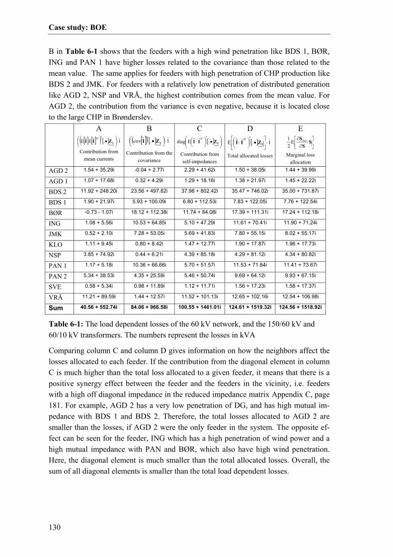
Case study: BOE
130
B in Table 6-1 shows that the feeders with a high wind penetration like BDS 1, BØR, ING and PAN 1 have higher losses related to the covariance than those related to the mean value. The same applies for feeders with high penetration of CHP production like BDS 2 and JMK. For feeders with a relatively low penetration of distributed generation like AGD 2, NSP and VRÅ, the highest contribution comes from the mean value. For AGD 2, the contribution from the variance is even negative, because it is located close to the large CHP in Brønderslev.
Comparing column C and column D gives information on how the neighbors affect the losses allocated to each feeder. If the contribution from the diagonal element in column C is much higher than the total loss allocated to a given feeder, it means that there is a positive synergy effect between the feeder and the feeders in the vicinity, i.e. feeders with a high off diagonal impedance in the reduced impedance matrix Appendix C, page 181. For example, AGD 2 has a very low penetration of DG, and has high mutual im-pedance with BDS 1 and BDS 2. Therefore, the total losses allocated to AGD 2 are smaller than the losses, if AGD 2 were the only feeder in the system. The opposite ef-fect can be seen for the feeder, ING which has a high penetration of wind power and a high mutual impedance with PAN and BØR, which also have high wind penetration. Here, the diagonal element is much smaller than the total allocated losses. Overall, the sum of all diagonal elements is smaller than the total load dependent losses.
A [ ] [ ]( ) [ ] 1.EE
*⋅
• IZII
H
Contribution from mean currents
B [ ]( ) [ ] 1.cov
*⋅
• IZI
Contribution from the covariance
C [ ]
•
⋅ IZII .Ediag
*H
Contribution from self-impedances
D
[ ] 1.E*
⋅
•
⋅ IZII
H
Total allocated losses
E
∂∂
SS
S lossE21
Marginal loss allocation
AGD 2 1.54 + 35.29i -0.04 + 2.77i 2.29 + 41.62i 1.50 + 38.05i 1.44 + 39.99i
AGD 1 1.07 + 17.68i 0.32 + 4.29i 1.29 + 18.16i 1.38 + 21.97i 1.45 + 22.22i
BDS 2 11.92 + 248.20i 23.56 + 497.82i 37.98 + 802.42i 35.47 + 746.02i 35.00 + 731.87i
BDS 1 1.90 + 21.97i 5.93 + 100.09i 6.80 + 112.53i 7.83 + 122.05i 7.76 + 122.54i
BØR -0.73 - 1.07i 18.12 + 112.38i 11.74 + 84.08i 17.39 + 111.31i 17.24 + 112.18i
ING 1.08 + 5.56i 10.53 + 64.85i 5.10 + 47.29i 11.61 + 70.41i 11.90 + 71.24i
JMK 0.52 + 2.10i 7.28 + 53.05i 5.69 + 41.83i 7.80 + 55.15i 8.02 + 55.17i
KLO 1.11 + 9.45i 0.80 + 8.42i 1.47 + 12.77i 1.90 + 17.87i 1.96 + 17.73i
NSP 3.85 + 74.92i 0.44 + 6.21i 4.39 + 85.18i 4.29 + 81.12i 4.34 + 80.82i
PAN 1 1.17 + 5.18i 10.36 + 66.66i 5.70 + 51.57i 11.53 + 71.84i 11.41 + 73.67i
PAN 2 5.34 + 38.53i 4.35 + 25.59i 5.46 + 50.74i 9.69 + 64.12i 9.93 + 67.15i
SVE 0.58 + 5.34i 0.98 + 11.89i 1.12 + 11.71i 1.56 + 17.23i 1.58 + 17.37i
VRÅ 11.21 + 89.59i 1.44 + 12.57i 11.52 + 101.13i 12.65 + 102.16i 12.54 + 106.98i
Sum 40.56 + 552.74i 84.06 + 966.58i 100.55 + 1461.01i 124.61 + 1519.32i 124.56 + 1518.92i
Table 6-1: The load dependent losses of the 60 kV network, and the 150/60 kV and 60/10 kV transformers. The numbers represent the losses in kVA

Case study: BOE
131
6.5.1.2 The influence of reactive power flows Table 6-2 shows the division of the losses in a part caused by the active power flows and a part caused by the reactive power flows. Column A and C have been calculated as described in section 3.3.3 page 47, and column B and D have been calculated using the sensitivities as described in section 3.2.1 page 35. The total sum of losses allocated to the reactive power flows is similar for the two methods, but for the individual busses, the two methods give diverging results for the reactive power contribution in column C and D. The problem with the current injection method here is that it assumes that the part of the current which is perpendicular to the bus voltage is related to the reactive power flow. The current injections, however, change the bus voltages. The sensitivity analysis considers the voltage changes imposed by a marginal change in reactive power, but the factor of 0.5 does not give an accurate measure of the actual effect of the total reactive power injection. With both methods, it is found that the reactive power injections only causes approxi-mately 5 % of the load dependent losses at the 60 kV level and above. A
( ) [ ] 1.E*
⋅
•⋅ IPP ZII H
Contribution from active power flows
B
∂∂
PPlossS
E21
Marginal allocation based on active
power
C
( ) [ ][ ] 1.E*
⋅•⋅ IQQ ZII H +
( ) [ ] 1.E*
⋅
•⋅+⋅ IQPPQ ZIIII HH
Contribution from reactive power flows including the cross effect
D
∂∂
QQlossS
E21
Marginal allocation
based on reactive power
AGD 2 1.38 + 35.41i 1.36 + 36.25i 0.13 + 2.64i 0.08 + 3.74i
AGD 1 1.28 + 20.42i 1.27 + 20.90i 0.10 + 1.55i 0.18 + 1.32i
BDS 2 33.95 + 712.81i 33.91 + 716.06i 1.52 + 33.21i 1.08 + 15.81i
BDS 1 7.73 + 120.32i 7.67 + 119.82i 0.10 + 1.74i 0.09 + 2.71i
BØR 16.69 + 107.83i 16.61 + 107.49i 0.70 + 3.48i 0.63 + 4.69i
ING 10.85 + 64.73i 10.87 + 65.64i 0.76 + 5.69i 1.03 + 5.60i
JMK 7.55 + 52.97i 7.53 + 53.61i 0.25 + 2.19i 0.50 + 1.57i
KLO 1.61 + 15.24i 1.61 + 15.50i 0.29 + 2.64i 0.35 + 2.23i
NSP 3.78 + 71.69i 3.77 + 72.35i 0.51 + 9.43i 0.57 + 8.47i
PAN 1 11.01 + 68.54i 10.94 + 69.25i 0.52 + 3.29i 0.47 + 4.42i
PAN 2 9.33 + 61.73i 9.43 + 64.55i 0.36 + 2.39i 0.50 + 2.60i
SVE 1.50 + 16.61i 1.50 + 16.81i 0.07 + 0.62i 0.08 + 0.55i
VRÅ 11.84 + 96.43i 11.94 + 99.07i 0.81 + 5.73i 0.60 + 7.91i
Sum 118.48 + 1444.72i 118.41 +1457.3i 6.13 + 74.60i 6.15 + 61.61i
Table 6-2: Separation in contributions from active and reactive power flows [kVA]

Case study: BOE
132
6.5.1.3 The influence of the cross effects Table 6-3 shows the effect of the cross terms in (3.12), page 32 which is used for sepa-ration of the load dependent losses from the no load losses, and (3.38), page 47 which is used to separate the losses, caused by the active power transfer from the losses, caused by the reactive power transfer. As shown later in Table 6-6, there is a surplus of ap-proximately 2.3 MVAr in the 60 kV system including the 60/10 kV transformers, when it is not loaded, due to the capacitive currents of the power lines. This means that sub stations which have a reactive power surplus, like BSD2 where a large CHP is con-nected, get positive losses assigned in Column A. On the other hand, a station with a lot of wind power production like Børglum gets negative losses assigned here. Compared to the total losses, these cross terms are rather small, and they partly cancel each other out. It can be seen that the cross terms in column B are rather small, even compared to the losses allocated to the reactive power transfer in Table 6-2, Column C.
6.5.1.4 10 and 0.4 kV network As shown in Figure 6-14, the 10 kV lines and the 10 / 0.4 kV transformers make the largest part of the total system losses. It is therefore relevant to allocate these losses to load and distributed generation. In this particular system, most of the larger wind farms and CHPs are connected to the 60 / 10 kV stations through their own 10 kV radials. There are, however, some small wind turbines and CHPs located along a feeder with consumers. To get the big picture of the losses, a regression model, containing only the
A
( ) ( ) SL21I VKI ⋅ℑ•⋅⋅ ][.E2*
j Cross effect between current and voltage
B
( ) [ ] 1.E*
⋅
•⋅+⋅ IQPPQ ZIIII HH
Cross effect between active and reac-tive current
AGD 2 -0.2656 + 1.3394i 0.0237 + 0.2922i
AGD 1 0.1767 + 0.7263i -0.0273 - 0.3168i
BDS 2 0.5625 - 4.0464i -0.0452 - 1.3425i
BDS 1 -0.1963 - 1.0730i 0.0285 + 0.2515i
BØR -0.5261 - 0.7837i 0.0570 + 0.2645i
ING 0.4633 + 0.8607i -0.0145 - 0.2574i
JMK 0.4995 + 0.5038i -0.0408 - 0.2078i
KLO 0.1688 + 0.3262i -0.0093 - 0.3366i
NSP 0.2837 + 1.0741i -0.0287 - 1.1288i
PAN 1 -0.4859 + 0.9775i 0.0099 + 0.0112i
PAN 2 0.1318 + 3.6497i -0.0237 - 0.3138i
SVE 0.0355 + 0.2576i -0.0030 - 0.0893i
VRÅ -0.8769 + 3.3128i 0.0786 + 0.4824i
Sum -0.0291 + 7.1249i 0.0052 - 2.6910i
Table 6-3: The two different cross effects [kVA]

Case study: BOE
133
terms in (3.25) page 43 where j=i, is performed for each feeder. Instead of the currents, the apparent power of all loads, all wind turbines and all CHPs have been inserted.
Table 6-5 shows the losses allocated to the different categories. For all the feeders, the regression coefficient, R, is higher than 95 % both for active and for reactive power which means that the regressive model can describe 95 % of the actual variation. It can be seen that the no-load losses make approximately half the losses of the feeders. In AGD 2 and JMK where only a few small DG units are located at feeders along radials with loads, the allocated losses are negative which means that these units actually con-tribute to reduction of the losses. Although the mean production from the CHPs is 65 % larger than from the wind turbines, the total losses allocated to the wind turbines are over twice the losses allocated to the CHPs. There are two main reasons for that. Firstly, all the wind turbines comprise a step up transformer, where as most of the larger CHPs are connected directly to the 10 kV network (or the transformer is not modeled). Sec-ondly, nearly half the CHP production comes from the Brønderslev KVV which is lo-cated only half a kilometer from the substation, BDS 1. Thirdly, the ratio between the mean value and the standard deviation of the production is higher for the CHPs than for the wind turbines. The high correlation between the CHP production and the load de-mand is not assumed to have a large impact on the losses at 10 kV level and below, since most of the large CHPs have their own radials.
A Load
B Wind
C CHP
D Sum
AGD 2 -2.17 0 0.1 -2.07 AGD 1 -1.62 0.13 0.4 -1.09 BDS 2 0 0 7.72 7.72 BDS 1 -2.96 3.1 1.97 2.11 BØR -3.09 3.26 0.62 0.79 ING -2.28 1.37 0.6 -0.31 JMK -2.69 0.03 2.51 -0.16 KLO -1.34 0.03 0.68 -0.63 NSP -3.1 0.05 0 -3.05 PAN 1 -2 1.66 0 -0.34 PAN 2 -2.29 0.22 0.52 -1.55 SVE -1.39 0.05 0.81 -0.53 VRÅ -3.73 0.04 0.56 -3.13 Sum -28.66 9.93 16.48 -2.25
Table 6-4: Mean values of active power contributions of each feeder [MW]
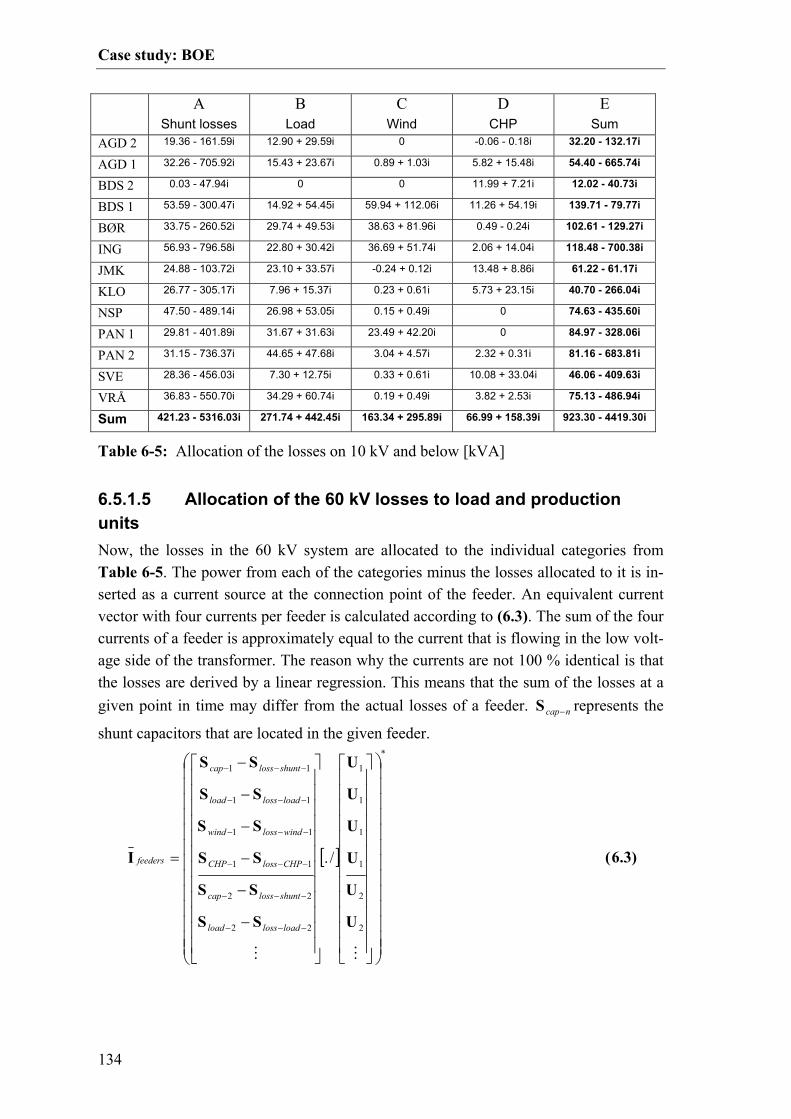
Case study: BOE
134
6.5.1.5 Allocation of the 60 kV losses to load and production units Now, the losses in the 60 kV system are allocated to the individual categories from Table 6-5. The power from each of the categories minus the losses allocated to it is in-serted as a current source at the connection point of the feeder. An equivalent current vector with four currents per feeder is calculated according to (6.3). The sum of the four currents of a feeder is approximately equal to the current that is flowing in the low volt-age side of the transformer. The reason why the currents are not 100 % identical is that the losses are derived by a linear regression. This means that the sum of the losses at a given point in time may differ from the actual losses of a feeder. ncap−S represents the
shunt capacitors that are located in the given feeder.
[ ]
*
2
2
1
1
1
1
22
22
11
11
11
11
/.
−
−
−
−
−
−
=
−−−
−−−
−−−
−−−
−−−
−−−
MM
U
U
U
U
U
U
SS
SS
SS
SS
SS
SS
I
loadlossload
shuntlosscap
CHPlossCHP
windlosswind
loadlossload
shuntlosscap
feeders ( 6.3)
A Shunt losses
B Load
C Wind
D CHP
E Sum
AGD 2 19.36 - 161.59i 12.90 + 29.59i 0 -0.06 - 0.18i 32.20 - 132.17i
AGD 1 32.26 - 705.92i 15.43 + 23.67i 0.89 + 1.03i 5.82 + 15.48i 54.40 - 665.74i
BDS 2 0.03 - 47.94i 0 0 11.99 + 7.21i 12.02 - 40.73i
BDS 1 53.59 - 300.47i 14.92 + 54.45i 59.94 + 112.06i 11.26 + 54.19i 139.71 - 79.77i
BØR 33.75 - 260.52i 29.74 + 49.53i 38.63 + 81.96i 0.49 - 0.24i 102.61 - 129.27i
ING 56.93 - 796.58i 22.80 + 30.42i 36.69 + 51.74i 2.06 + 14.04i 118.48 - 700.38i
JMK 24.88 - 103.72i 23.10 + 33.57i -0.24 + 0.12i 13.48 + 8.86i 61.22 - 61.17i
KLO 26.77 - 305.17i 7.96 + 15.37i 0.23 + 0.61i 5.73 + 23.15i 40.70 - 266.04i
NSP 47.50 - 489.14i 26.98 + 53.05i 0.15 + 0.49i 0 74.63 - 435.60i
PAN 1 29.81 - 401.89i 31.67 + 31.63i 23.49 + 42.20i 0 84.97 - 328.06i
PAN 2 31.15 - 736.37i 44.65 + 47.68i 3.04 + 4.57i 2.32 + 0.31i 81.16 - 683.81i
SVE 28.36 - 456.03i 7.30 + 12.75i 0.33 + 0.61i 10.08 + 33.04i 46.06 - 409.63i
VRÅ 36.83 - 550.70i 34.29 + 60.74i 0.19 + 0.49i 3.82 + 2.53i 75.13 - 486.94i
Sum 421.23 - 5316.03i 271.74 + 442.45i 163.34 + 295.89i 66.99 + 158.39i 923.30 - 4419.30i
Table 6-5: Allocation of the losses on 10 kV and below [kVA]

Case study: BOE
135
Since the virtual current sources are connected directly at the collection point of the feeder, the mutual impedances between them are equal to the individual self-impedances. This means that the reduced impedance matrix must be expanded accord-ing to (6.4).
=−
OMMMMMM
K
K
K
K
K
K
222221212121
222221212121
121211111111
121211111111
121211111111
121211111111
IIIIII
IIIIII
IIIIII
IIIIII
IIIIII
IIIIII
feeders
ZZZZZZ
ZZZZZZ
ZZZZZZ
ZZZZZZ
ZZZZZZ
ZZZZZZ
ZI ( 6.4)
Using (6.3) and (6.4) to perform the same calculation as in Table 6-1 column D yields the data in Table 6-6. Column E contains the sum of all losses allocated to each feeder. This should be equal to column D in Table 6-1. There is a deviation of a few percent, since the losses are not 100 % accurately estimated by the linear regression method. The row with the label 60 kV denotes the shunt losses at 60 kV level and above.
In some of the feeders with a low penetration of DG, negative losses are allocated to the CHPs and / or the wind turbines, because they can supply the load demand at their own feeder or in the neighboring feeders. In the feeder, BDS 1 where there is a high penetra-
A Shunt losses
B Load
C Wind
D CHP
E Sum
AGD 2 -0.06 - 1.31i 1.59 + 40.64i 0 -0.04 - 1.47i 1.49 + 37.85i
AGD 1 0.41 + 6.42i 1.05 + 18.28i 0.01 - 0.40i -0.08 - 2.33i 1.38 + 21.97i
BDS 2 0.02 + 0.42i 0 0 35.49 + 746.25i 35.51 + 746.67i
BDS 1 -0.06 - 1.11i -3.30 - 36.86i 8.68 + 129.08i 2.52 + 30.94i 7.83 + 122.06i
BØR -0.13 - 0.11i 5.33 + 7.00i 11.26 + 93.63i 0.62 + 10.44i 17.09 + 110.95i
ING 0.77 + 10.75i 6.12 + 25.03i 5.01 + 33.81i -0.49 + 0.26i 11.42 + 69.86i
JMK 0.39 + 4.59i 4.73 + 6.65i 0.12 + 0.48i 2.56 + 43.42i 7.80 + 55.13i
KLO 0.67 + 6.04i 1.21 + 8.78i -0.02 + 0.01i 0.05 + 3.07i 1.92 + 17.90i
NSP 1.47 + 28.15i 2.87 + 53.56i -0.05 - 0.74i 0 4.29 + 80.97i
PAN 1 0.17 + 0.41i 4.84 + 21.20i 6.43 + 50.00i 0 11.44 + 71.61i
PAN 2 0.37 + 3.85i 8.17 + 57.61i 0.42 - 0.35i 0.62 + 2.71i 9.58 + 63.82i
SVE 0.25 + 2.00i 1.12 + 9.94i -0.02 + 0.19i 0.23 + 5.06i 1.58 + 17.20i
VRÅ -0.99 - 7.13i 14.03 + 113.03i 0.00 - 0.35i -0.53 - 3.89i 12.51 + 101.65i
60 kV 221.25 - 2299.95i 0 0 0 221.25 - 2299.95i
Sum 224.53 - 2246.98i 47.76 + 324.86i 31.84 + 305.35i 40.95 + 834.46i 345.08 - 782.32i
Table 6-6: Allocation of the losses on 60 kV and above in kVA

Case study: BOE
136
tion of DG, negative losses are allocated to the load, because it limits the upwards po-wer flow in periods. Table 6-7 contains the sum of Table 6-5 and Table 6-6. The sum of all the elements in Table 6-7 is approximately equal to the mean value of the total system losses. The mean value of the total system losses for the period, calculated by PowerFactory®, is 1.2679-j 5163.9 kVA. The lower row of the table represents the losses allocated to each of the categories. To put the losses that have been allocated to the different categories into context, they have been presented in Table 6-8 as percentages of the total power flows and of the total system losses. Only the load dependent losses are allocated to participants with the loss allocation methods used above. Therefore, the no-load losses of the transformers related to the loads, wind turbines and CHPs have been added to the losses allocated to the respective categories.
A Shunt losses
B Load
C Wind
D CHP
E Sum
AGD 2 19.30 - 162.90i 14.49 + 70.23i 0 -0.11 - 1.65i 33.69 - 94.32i
AGD 1 32.67 - 699.50i 16.48 + 41.95i 0.89 + 0.63i 5.74 + 13.15i 55.78 – 643.77i
BDS 2 0.05 - 47.52i 0 0 47.48 + 753.46i 47.53 + 705.94i
BDS 1 53.53 - 301.57i 11.62 + 17.59i 68.62 + 241.14i 13.78 + 85.13i 147.54 + 42.29i
BØR 33.63 - 260.64i 35.07 + 56.52i 49.90 + 175.59i 1.11 + 10.20i 119.70 – 18.32i
ING 57.71 - 785.83i 28.92 + 55.46i 41.70 + 85.56i 1.57 + 14.31i 129.89 - 630.51i
JMK 25.27 - 99.13i 27.82 + 40.22i -0.12 + 0.60i 16.05 + 52.27i 69.02 - 6.03i
KLO 27.44 - 299.12i 9.17 + 24.15i 0.21 + 0.62i 5.79 + 26.22i 42.62 – 248.13i
NSP 48.96 - 460.99i 29.85 + 106.62i 0.10 - 0.25i 0 78.91 – 354.63i
PAN 1 29.98 - 401.49i 36.51 + 52.83i 29.92 + 92.20i 0 96.41 – 256.45i
PAN 2 31.52 - 732.53i 52.82 + 105.29i 3.46 + 4.22i 2.94 + 3.03i 90.74 – 619.99i
SVE 28.61 - 454.02i 8.41 + 22.68i 0.31 + 0.80i 10.31 + 38.10i 47.64 – 392.44i
VRÅ 35.84 - 557.83i 48.32 + 173.77i 0.19 + 0.13i 3.29 - 1.37i 87.64 – 385.29i
60 kV 221.25 - 2299.95i 0 0 0 221.25 - 2299.95i
Sum 645.76 - 7563.01i 319.50 + 767.31i 195.18 + 601.24i 107.94 + 992.84i 1268.38 - 5201.6i
Table 6-7: Allocation of all the losses in kVA
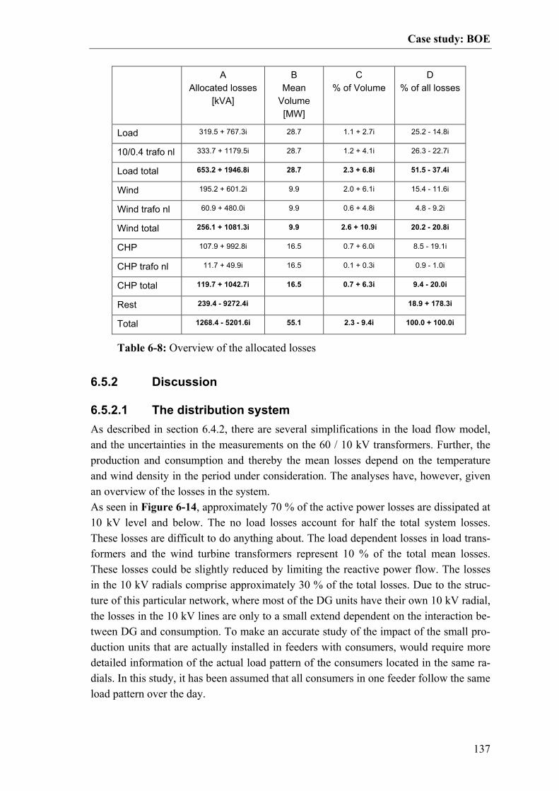
Case study: BOE
137
6.5.2 Discussion
6.5.2.1 The distribution system As described in section 6.4.2, there are several simplifications in the load flow model, and the uncertainties in the measurements on the 60 / 10 kV transformers. Further, the production and consumption and thereby the mean losses depend on the temperature and wind density in the period under consideration. The analyses have, however, given an overview of the losses in the system. As seen in Figure 6-14, approximately 70 % of the active power losses are dissipated at 10 kV level and below. The no load losses account for half the total system losses. These losses are difficult to do anything about. The load dependent losses in load trans-formers and the wind turbine transformers represent 10 % of the total mean losses. These losses could be slightly reduced by limiting the reactive power flow. The losses in the 10 kV radials comprise approximately 30 % of the total losses. Due to the struc-ture of this particular network, where most of the DG units have their own 10 kV radial, the losses in the 10 kV lines are only to a small extend dependent on the interaction be-tween DG and consumption. To make an accurate study of the impact of the small pro-duction units that are actually installed in feeders with consumers, would require more detailed information of the actual load pattern of the consumers located in the same ra-dials. In this study, it has been assumed that all consumers in one feeder follow the same load pattern over the day.
A Allocated losses
[kVA]
B Mean
Volume [MW]
C % of Volume
D % of all losses
Load 319.5 + 767.3i 28.7 1.1 + 2.7i 25.2 - 14.8i
10/0.4 trafo nl 333.7 + 1179.5i 28.7 1.2 + 4.1i 26.3 - 22.7i
Load total 653.2 + 1946.8i 28.7 2.3 + 6.8i 51.5 - 37.4i
Wind 195.2 + 601.2i 9.9 2.0 + 6.1i 15.4 - 11.6i
Wind trafo nl 60.9 + 480.0i 9.9 0.6 + 4.8i 4.8 - 9.2i
Wind total 256.1 + 1081.3i 9.9 2.6 + 10.9i 20.2 - 20.8i
CHP 107.9 + 992.8i 16.5 0.7 + 6.0i 8.5 - 19.1i
CHP trafo nl 11.7 + 49.9i 16.5 0.1 + 0.3i 0.9 - 1.0i
CHP total 119.7 + 1042.7i 16.5 0.7 + 6.3i 9.4 - 20.0i
Rest 239.4 - 9272.4i 18.9 + 178.3i
Total 1268.4 - 5201.6i 55.1 2.3 - 9.4i 100.0 + 100.0i
Table 6-8: Overview of the allocated losses

Case study: BOE
138
As seen in Table 6-1 the load dependent losses at 60 kV and above including the 60 / 10 kV transformers only add up to 125 kW or approximately 10 % of the total losses. These are, however, the most interesting part of the losses, since they actually depend on the interaction between DG and consumption. The variance and covariance account for 84 kW of these losses. Maintaining the same mean production and consumption, this number would be the highest theoretical loss reduction, if the distributed generation could be synchronized perfectly with the load. Generally, it seems that the network is relatively strong, and the total losses (without the 0.4 kV lines) of 2.5 % of the total mean transfer volume is considered reasonable.
6.5.2.2 The algorithms The analysis has been performed using the methods described in Chapter 3 except for the flow tracing algorithm. For the 60 kV system the results from current injection method have been compared to results from the sensitivity analysis, and the two algo-rithms show identical results. The advantages of the sensitivity analysis are firstly that the algorithm is a part of most power system simulation tools. In PowerFactory® the calculation of loss sensitivities, however, requires an invocation of the sensitivity tool for each bus under consideration. This can be automated, but it extends the total simula-tion time. Secondly, the interpretation is well suited for e.g. incentive generating price signals, since it directly gives the price of a small change in production / consumption. The advantages of the current injection method are firstly that it is based on the reduced impedance matrix, which makes it more intuitive to work with. If no complete model is available, the diagonal elements can for example be estimated with the short circuit power, and the mutual impedances can be approximated with the short circuit power at the point of common coupling. If the position of the tap changers is assumed to be con-stant, the reduced impedance matrix is constant. This makes it possible to make a rough estimate of the cost of transferring power from one place to another just by looking at the impedance matrix. Secondly, the algorithm makes it possible to study the cross ef-fects between different current infeeds and the effect from the mean values of the in-feeds can easily be separated from the effect of the covariances. Like the sensitivity analysis, the algorithm requires a load flow calculation per measurement point to deter-mine the current infeeds. PowerFactory® does not directly support the export of the impedance matrix. It is, however, possible that it could get implemented in a future ver-sion of the tool. The linear regression method is a simple way of getting an overview of the losses at 10 kV and below. It is, however, not possible to separate the losses related to one wind farm from the losses related to another wind farm in the same feeder due to the multi-collinearity problem.

Case study: BOE
139
6.6 Reactive power compensation As described in Section 5.2, page 95 ff, the distribution network operator is obliged to keep the reactive power transfer with the transmission system within a given band. For the 150 / 60 kV transformer station in Nibstrup, the reactive power flow upwards, measured at the 60 kV side must be below 9 MVAr 99 percent of a year, and the flow downwards must be below 2 MVAr 99 % of the year [128]. Figure 6-16 shows the duration curves of the reactive flow at the 60 kV side of the transformer station based on the simulated and the measured values for the ten month period under consideration. The 1 and 99 % fractiles have been marked with vertical lines. As mentioned in Section 6.4.6, there is some discrepancy between the measured and the simulated reactive power flows, which can partly be caused by measurement
inaccuracies and partly by modeling inaccuracies. For the reactive power export, both the measured and the simulated values indicate that the limit is held. The simulated values indicate an export of 8.5 MVAr at the 1 % frac-tile. For reactive power import, the measured values give 5 MVAr at the 99 % fractile while the simulated values only give 3.2 MVAr, which is in both cases over the permit-ted 2 MVAr. It would be a good idea to calibrate the measurement equipment of the transformer, before further optimizations are of the compensation strategy are made. In the following, the simulated values are used rather than the measured, because they are consistent with the rest of the simulation.
Figure 6-16: Duration curves for reactive power exchange on the 60 kV side of the 150 / 60 kV transformers. The sign is considered positive for import to the distribution system.

Case study: BOE
140
6.6.1 Compensation strategy The sinks and sources of reactive power in the system are outlined in Figure 6-15, page 128. The controllable reactive power resources comprise a 2.4 MVAr one step capacitor battery which is connected at the 10 kV level in Nibstrup and CHPs with a total rated power of 50 MW. The Capacitor battery is operated based on the measured reactive power flow in the 150/60 kV transformers. According to [14], new CHPs with a rated power over 1.5 MW must be able to operate with a value of tan(φ) between -0.2 and 0.4 at the rated production capacity. Currently, the CHPs operate with time dependent tan(φ). Reference [61] presents simulations made for the BOE system, where the 4.8 MVAr of fixed capacitors connected to the 10 kV system have been replaced with 11 MVAr of switchable capacitors. The switchable capacitor batteries are connected at the 10 kV side of the sub station in Børglum, Pandrup and Nibstrup (See Figure 6-1, page 113). The battery in Nibstrup is controlling the flow in the 150/60 kV transformer and the batteries in Børglum and Pandrup are controlling the reactive power flow in the 60 kV lines going east. The power factor of the CHPs has been adjusted to cover the variance of the load. This strategy has the advantage that it does not require communication be-tween the different components. The drawback is that the batteries in the western part of the network and the CHPs will in some situations deliver reactive power while the dis-tribution network is exporting reactive power. An alternative way of solving the problem is to have a central control unit which dis-patches the reactive power among the available capacitor batteries and CHPs in an op-timal manner under consideration of generator capacity, voltage constraints, losses etc. A way of optimizing the reactive power compensation in a distribution system with dis-persed generation has been presented in [21]. The maximal potential reduction in exchange of reactive power with the transmission system, given that two way communication is available to all CHP units, has roughly been estimated by analyzing the simulation results in Matlab®. The approach is to firstly calculate the reactive power that would have flown if the CHPs were running at unity power factor, and the capacitor battery were out of service by adding the reactive power that has been provided by the CHPs and the capacitor battery to the simulated reactive power import on the 60 kV side of the transmission transformers. Secondly, an alternative dispatch of reactive power is calculated the following way. If the import is larger than 1.2 MVAr, 2.4 MVAr is subtracted from the imported reactive power. The remaining reactive power flow is dispatched among the CHPs that are operating at a given time under consideration of limits for tan(φ). Because the generators are only op-erated close to their rated power, the reactive power capability of all CHPs can be calcu-lated based on the total output of the CHPs. With this simplified approach, the change in reactive power losses, caused by the change in reactive power flows and the voltage magnitude constraints are not taken into account.

Case study: BOE
141
The estimated duration curves for different control intervals are depicted in Figure 6-17. If the CHPs were all operated at unity power factor, the 99 % fractile for the reac-tive power import would be at 11 MVAr. To meet the requirement of a maximal import of 2 MVAr would require approximately 9 MVAr of extra switchable capacitors. The difference between setting the upper limit of tan(φ) to 0.3 and 0.4 is only 1 MVAr at the 99 % fractile. Allowing the CHPs to absorb reactive power with a tan(φ) of -0.2 only makes a difference of 0.6 MVAr at the 1 % fractile, because the remaining reactive power export occurs when the CHPs are not operating.
The major potential improvement with a centralized control scheme is that the reactive power production of the CHPs can be limited in periods where there is a surplus of reac-tive power. Figure 6-18 shows the time dependency of the reactive power production of the CHPs for the actual simulation and for different limits for tan(φ). The mean values of reactive power are smaller for the alternative compensation strategies than for the actual strategy at all times, and especially between 15:30 and 20:00 and in the weekends and holidays.
Figure 6-17: Duration curves for reactive power exchange on the 60 kV side of the 150 / 60 kV transformer. The sign is considered positive for im-port to the distribution system.

Case study: BOE
142
It has been shown that it is possible to reduce the exchange of reactive power with the transmission system by performing a centralized control of the CHPs. For a real implementation, it would be most efficient to include the biggest CHPs only. There is already communication between the control room and the 22 MW CHP in Brønderslev, and discussions have been made bout using this plant for controlling the reactive power exchange. If the exchange band is to be narrowed further, a possibility would be to exchange some of the 10 kV fixed capacitors with switchable batteries. After 2008, fiber connections are made between the control room and all the 60 / 10 kV sub stations. This will make it possible to perform a centralized control of capacitor batteries located there. Before doing extra investments related to this, the accuracy of the online measurement system of the transmission transformers should be verified. In a centralized control system, it would be a good idea to reserve some dynamic control capacity of the CHPs for situations with abnormally high or low voltage. Further, each of the CHPs should have a time dependent tan(φ) curve as backup in case of communi-cation failure over a period.
6.7 Wind turbine connection point To illustrate some of the theory regarding the influence of the network strength on volt-age profiles and transient stability, the connection point of the 4.5 MW wind farm Ny Alstrup is closer examined. The wind farm comprises six 0.75 MW no load compen-
( ) [ ]2.0;0tan ∈φ
( ) [ ]3.0;1.0tan −∈φ
( ) [ ]4.0;2.0tan −∈φ
simulation Actual
( ) [ ]2.0;0tan ∈φ
( ) [ ]3.0;1.0tan −∈φ
( ) [ ]4.0;2.0tan −∈φ
simulation Actual
Figure 6-18: Delivered reactive power of the CHPs with the different com-pensation strategies. The solid curves denote mean values of each time in-terval.

Case study: BOE
143
sated Danish Concept wind turbines, and it is connected to the 60 / 10 kV station Ing-strup through an 8 km radial – see Figure 6-19.
The active and reactive power of the wind farm is measured by the SCADA system at the Ingstrup sub station at the connecting radial. The power production of the individual wind turbines has been set by correcting for the losses in the radial, and the transform-ers. The 80 kW load which is located at Bus A has not been considered further in the following analyses, since it is relatively small compared to the wind farm.
G~G~G~
G~G~G~
ING 10 kVBus A Bus B WT 0 H
WT 0 L WT 1 L WT 2 L
WT 1 H WT 2 H
WT 3 H
WT 3 L
WT 4 H
WT 4 L
WT 5 H
WT 5 L
0.75 MW 0.75 MW 0.75 MW
0.75 MW 0.75 MW 0.75 MW
2.3 km 2.3 km 3.2 km
80 kW
G~G~G~
G~G~G~
ING 10 kVBus A Bus B WT 0 H
WT 0 L WT 1 L WT 2 L
WT 1 H WT 2 H
WT 3 H
WT 3 L
WT 4 H
WT 4 L
WT 5 H
WT 5 L
0.75 MW 0.75 MW 0.75 MW
0.75 MW 0.75 MW 0.75 MW
2.3 km 2.3 km 3.2 km
80 kW
Figure 6-19: Connection of the 4.5 MW wind farm Ny Alstrup to the Ingstrup 60/10 kV station

Case study: BOE
144
6.7.1 Short circuit capacity The short circuit power at the stations along the way to the wind turbine has been plot-ted in Figure 6-20. The calculations were made with the stationary short circuit tool of PowerFactory® as described in section 4.1, page 55. During the calculations, all loads and generators were disabled, and the tap changers were set to their average position.
The location of the 60 / 10 kV stations can be seen in the map in Figure 6-1, page 113. The short circuit power at the connection point of the wind farm, WT 0 H, is 46 MVA. Assuming a power factor of 0.87 as for the wind turbine in Appendix B, the short circuit ratio for the entire wind farm would be 46 MVA · 0.87 / 4.5 MW = 8.9. This can be considered a reasonable network strength. Figure 6-21 shows the Thevenin impedances at the same sub stations. It can be seen that the contribution from the 60 kV network to the Thevenin impedance is very small compared to the contribution from the transformers and the 10 kV network. The lowest X/R ratio, 1.4, is found at the bus, WT 5 H. At the low voltage side of the step up trans-former, the X/R ratio is 3.1 due to the leakage reactance of the transformer. It can be seen that the contribution from the 60 kV network to the impedance is relatively small compared to the low voltage network, and that the largest contribution to the reactive part or the impedance comes from the transformers while most of the resistive part comes from overhead lines and cables.
WT 5 L
WT 5 HWT 0 H
Ingstrup 10 kV
Ingstrup 60 kV
Børglum 60 kV Vrå 60 kV Nibstrup 60 kV
Pandrup 60 kV
Agdrup 60 kV
Brønderslev 60 kV
Bus B Bus A
WT 5 L
WT 5 HWT 0 H
Ingstrup 10 kV
Ingstrup 60 kV
Børglum 60 kV Vrå 60 kV Nibstrup 60 kV
Pandrup 60 kV
Agdrup 60 kV
Brønderslev 60 kV
Bus B Bus A
Figure 6-20: The short circuit power at different points along the way to the wind turbine WT 5

Case study: BOE
145
6.7.2 Voltage rise The voltage rise at the high voltage side of the step up transformer of the wind turbine, WT 5, has been analyzed based on the methods presented in Section 5.4, page 102 ff. The reason for looking at this particular bus is that it has the lowest X/R ratio of the busses in Figure 6-21. It is therefore expected that the highest voltage rise will occur there. The voltage at the 10 kV side of the transformer station in Ingstrup is controlled with an automatic tap changer with a step size of 1.6 %. It can therefore be assumed that the voltage there is within a given control band. Assuming that the voltage at the 10 kV bus of the Ingstrup sub station is independent of the production from the wind farm, the relevant impedance for assessment of the voltage rise is the impedance from WT 5 to ING 10 kV. Assuming that the other wind turbines in the wind farm contribute with approximately the same active and reactive power as WT 5, an equivalent impedance at the Bus, WT 5 H can be calculated using (4.22), page 63. The resulting impedance is thereby modified to cover the expected voltage change imposed by the other turbines. Table 6-9 shows the calculation of the relevant impedances. It has been assumed that the mutual impedance between WT 5 and the other wind turbines can be estimated with the self impedance at the point of common coupling between them. The mutual imped-ance between WT 5 and WT 0 – WT 2 can for example be estimated with self impedance at WT 0 H. The equivalent impedance, ZWT5H-mod is less than 6 times ZWT5H , because the other wind turbines do not contribute as much to the voltage rise as WT 5 does. To take
Ingstrup 10 kV
Ingstrup 60 kV
Børglum 60 kV Vrå 60 kV
Nibstrup 60 kV
Pandrup 60 kV
Agdrup 60 kV Brønderslev 60 kV
WT 5 L
WT 5 HWT 0 H
Bus BBus A
Ingstrup 10 kV
Ingstrup 60 kV
Børglum 60 kV Vrå 60 kV
Nibstrup 60 kV
Pandrup 60 kV
Agdrup 60 kV Brønderslev 60 kV
WT 5 L
WT 5 HWT 0 H
Bus BBus A
Figure 6-21: The Thevenin impedance at different points along the way to the wind turbine WT 5. The base of the p.u. conversion is 100 MVA
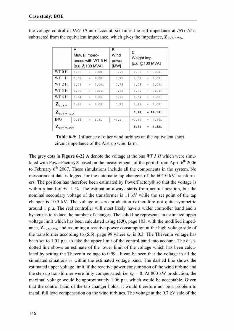
Case study: BOE
146
the voltage control of ING 10 into account, six times the self impedance at ING 10 is subtracted from the equivalent impedance, which gives the impedance, ZWT5H-ING.
The grey dots in Figure 6-22 A denote the voltage at the bus WT 5 H which were simu-lated with PowerFactory® based on the measurements of the period from April 6th 2006 to February 6th 2007. These simulations include all the components in the system. No measurement data is logged for the automatic tap changers of the 60/10 kV transform-ers. The position has therefore been estimated by PowerFactory® so that the voltage is within a band of +/- 1 %. The estimation always starts from neutral position, but the nominal secondary voltage of the transformer is 11 kV while the set point of the tap changer is 10.5 kV. The voltage at zero production is therefore not quite symmetric around 1 p.u. The real controller will most likely have a wider controller band and a hysteresis to reduce the number of changes. The solid line represents an estimated upper voltage limit which has been calculated using (5.9), page 103, with the modified imped-ance, ZWT5H-ING and assuming a reactive power consumption at the high voltage side of the transformer according to (5.5), page 99 where kQ is 0.3. The Thevenin voltage has been set to 1.01 p.u. to take the upper limit of the control band into account. The dash-dotted line shows an estimate of the lower limit of the voltage which has been calcu-lated by setting the Thevenin voltage to 0.99. It can be seen that the voltage in all the simulated situations is within the estimated voltage band. The dashed line shows the estimated upper voltage limit, if the reactive power consumption of the wind turbine and the step up transformer were fully compensated, i.e. kQ = 0. At 800 kW production, the maximal voltage would be approximately 1.06 p.u. which would be acceptable. Given that the control band of the tap changer holds, it would therefore not be a problem to install full load compensation on the wind turbines. The voltage at the 0.7 kV side of the
A Mutual imped-ances with WT 5 H [p.u.@100 MVA]
B Wind power [MW]
C Weight imp [p.u.@100 MVA]
WT 0 H 1.08 + 2.00i 0.75 1.08 + 2.00i WT 1 H 1.08 + 2.00i 0.75 1.08 + 2.00i WT 2 H 1.08 + 2.00i 0.75 1.08 + 2.00i WT 3 H 1.20 + 2.04i 0.75 1.20 + 2.04i WT 4 H 1.34 + 2.06i 0.75 1.34 + 2.06i
HWT 5Z 1.49 + 2.08i 0.75 1.49 + 2.08i
modHWT −5Z 7.28 + 12.18i ING 0.14 + 1.3i -4.5 -0.86 - 7.96i
INGHWT −5Z 6.41 + 4.22i
Table 6-9: Influence of other wind turbines on the equivalent short circuit impedance of the Alstrup wind farm.

Case study: BOE
147
transformer does not increase as much as the voltage of the high voltage side because of the higher X/R ratio.
Figure 6-22 B shows the allowable PQ range of the wind turbine, WT 5, including the transformer under consideration of voltage and current limits. The current limit has been calculated under the assumption that the bus voltage is 1 p.u. and that the rated power factor is 0.9. The upper and lower voltage limits have been calculated by inserting a Thevenin voltage of 1.01 p.u. and 0.99 p.u. and bus voltage limits of 1.06 p.u. and 0.94 p.u. in (5.21), page 108, and creating a plot similar to Figure 5-8. With the given volt-age and current limits, the upper voltage limit becomes the limiting factor for reactive power injection, when each of the wind turbines are producing more than 0.33 MW. The lower voltage at the 10 kV side of the transformer never imposes a limit for reactive power absorption. The reactive power absorption may, however, be limited by the volt-age on the 0.7 kV side of the transformer.
6.7.3 Voltage sensitivity In the previous section it was shown that the production from the wind farm does not cause the voltage at the bus with the lowest X/R ratio of the radial to exceed the upper limit. Another issue is voltage fluctuations resulting from fluctuating power production, also denoted as flicker. Methods for measurement and calculation of the flicker impact of wind turbines are specified in the IEC standard, 61400-21 [28]. This section will not focus on actual flicker assessment, but simply illustrate how power fluctuations impose voltage variations.
Current limit @ |V|=1 p.u.
Upper voltage limitVTh = 1.01 p.u. |V| = 1.06 p.u.
Lower voltage limitVTh = 0.99 p.u. |V |= 0.94 p.u.
Allowable PQ range
VTh = 0.99, kQ=0.3
VTh = 1.01 p.u., kQ=0.3VTh = 1.01 p.u., kQ=0
Detailed simulation
Current limit @ |V|=1 p.u.
Upper voltage limitVTh = 1.01 p.u. |V| = 1.06 p.u.
Lower voltage limitVTh = 0.99 p.u. |V |= 0.94 p.u.
Allowable PQ range
VTh = 0.99, kQ=0.3
VTh = 1.01 p.u., kQ=0.3VTh = 1.01 p.u., kQ=0
Detailed simulation
Figure 6-22: The simulated and estimated voltage at the bus WT 5 H

Case study: BOE
148
The influence of power variations of the wind farm on the voltage at the neighboring bus, Bus B, has been assessed. Presently, no load is connected to the bus, but it would be possible to do so in the future. The dots in Figure 6-23 denote the simulated voltage as a function of the total production of the wind farm. The maximal voltage rise is in this case only approximately 3 %. The solid curve shows the estimated voltage when the self impedance of Bus B minus the self impedance at the Ingstrup sub station is inserted in (5.9), page 103. The active and reactive power that has been inserted is the same as in the previous section. This means that active and reactive power losses from the high voltage side of the transformers to Bus B have been neglected. For small and fast variations of the production, the automatic tap changer will, however, not operate. This means that for small signal analyses, the voltage at the Ingstrup sub station cannot be assumed constant. This means that the entire self-impedance at the connection point should be used for assessment of the small signal voltage sensitivity. The dash-dotted line in Figure 6-23 shows the equivalent voltage profile if the entire self-impedance is used. It can be seen that it reaches its maximum at approximately half the rated production of the wind farm. This does not necessarily represent the voltage profile at the bus, if the tap changers were disabled, because the loads and the other pro-duction units also contribute to the voltage change, but it gives an indication of the dif-
ference between the large signal and the small signal behavior of the voltage. The dots in Figure 6-24 A and B show the partial voltage sensitivities to active and re-active power injections at Bus B. The sensitivities have been calculated with PowerFac-tory® during the simulation of the entire system. In principle the calculations are made according to (5.24), page 110. The generators and loads have been considered as PQ sources/sinks during the load flow calculations. Therefore the small signal dependency of the reactive power exchange on the voltage is not considered. The dash-dotted lines show the sensitivities, estimated with (5.10), (5.11) and (5.12) page 103 ff. Despite the fact that the estimates only consider the power flow imposed by the wind farm, there is a good agreement between the simulated and the estimated sensi-tivities.
Figure 6-23: The simulated and estimated voltage at Bus B

Case study: BOE
149
The total voltage sensitivity in Figure 6-24 C taking the reactive power consumption of the wind farm into account has been calculated using (5.15), page 105, both for the simulated and the estimated sensitivities. At low production from the wind farm, the sensitivity is approximately 0.7%/MW. At a total production of 2.5 MW, it can be seen that small variations in the production have no influence on the voltage at Bus B.
6.7.4 Losses In this section the losses caused by the production of active power and the absorption of reactive power at the connection point of the wind farm are investigated. During the detailed simulation, the loss sensitivities at the bus, WT 0 H which is the collection point of the wind farm have been calculated. The fundamental theory about loss sensitivities is presented in Section 3.2.1, page 35. Figure 6-25 A shows the partial derivative of the losses with respect to injection of an extra MW at the collection point of the wind farm. Up to a production of approximately 0.6 MW, the active power injection will in average contribute to reducing the total sys-tem losses, because the active power can supply the costumers connected to the Ingstrup sub station. At the maximal production, the marginal losses make approximately 10 %. The sensitivity of the losses to reactive power injections are depicted in Figure 6-25 B. At low production, the sensitivity is positive, which means that a marginal increase in reactive power absorption will reduce the total system losses, because there is a surplus
Figure 6-24: Voltage sensitivities for Bus B
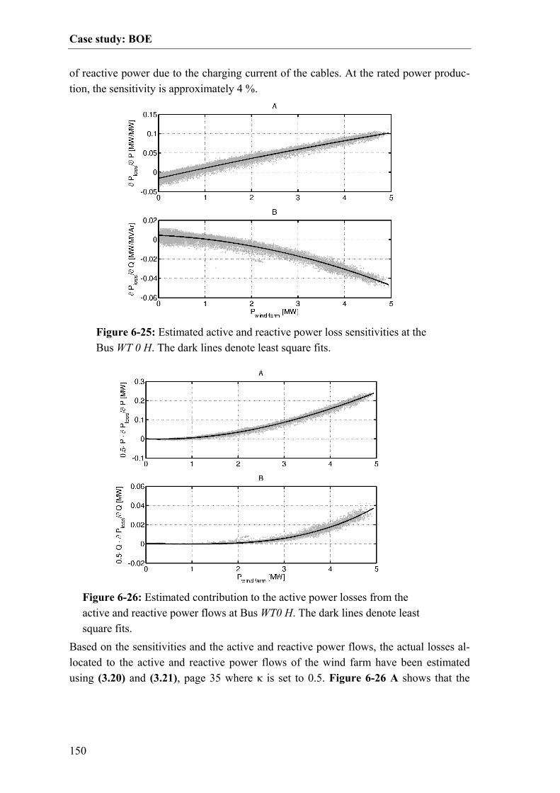
Case study: BOE
150
of reactive power due to the charging current of the cables. At the rated power produc-tion, the sensitivity is approximately 4 %.
Based on the sensitivities and the active and reactive power flows, the actual losses al-located to the active and reactive power flows of the wind farm have been estimated using (3.20) and (3.21), page 35 where κ is set to 0.5. Figure 6-26 A shows that the
Figure 6-25: Estimated active and reactive power loss sensitivities at the Bus WT 0 H. The dark lines denote least square fits.
Figure 6-26: Estimated contribution to the active power losses from the active and reactive power flows at Bus WT0 H. The dark lines denote least square fits.

Case study: BOE
151
losses caused by the active power transfer make approximately 200 kW at the rated pro-duction which corresponds to approximately 4.4 % of the actual power production. The losses allocated to the reactive power transfer in Figure 6-26 B make approxi-mately 25 kW at the rated production which is only 0.6 %, and the characteristic is much steeper than for the active power. The mean losses allocated to the active power in the period under consideration make 26.6 kW and the mean losses allocated to the reactive power losses comprise 2.4 kW. The mean production of the wind farm in the period is approximately 1.2 MW. The allocated losses only include the transfer from the collection point of the wind farm to the transmission system. The reason why the sensitivities were not calculated at the low voltage side of the step up transformers is that the power flow of the generator has been specified at the high voltage side of the step up transformers which means that the sensitivities at the low voltage side are per definition zero. The extra losses can be esti-mated by calculating an aggregated impedance for the whole wind farm, seen from the 0.7 kV side and comparing this impedance to the impedance at the collection point. The process of aggregating infeed points is described in Section 3.3.1.1, page 44 ff. The ba-sic assumption is that the total power of the wind farm can be represented with a linear combination of 6 currents injections. In the following, it has been assumed that the cur-rent injection is the same at the low voltage side of all the wind turbines, which leads to (6.5).
[ ]11111161
=HIK ( 6.5)
The self impedances and the mutual impedances at the 0.7 kV connection points of the wind turbines are given in per unit with 100 MVA base in (6.6). The mutual impedances have been set to the self impedances at the point of common coupling between the tur-bines.
++++++
++++++
++++++
++++++
++++++
++++++
=
8.0i2.602.1i1.342i1.202i1.082i1.082i1.08
2.1i1.348.0i2.452i1.202i1.082i1.082i1.08
2i1.202i1.207.9i2.312i1.082i1.082i1.08
2i1.082i1.082i1.087.9i2.482i1.232i1.08
2i1.082i1.082i1.082i1.237.9i2.342i1.08
2i1.082i1.082i1.082i1.082i1.087.9i2.19IZ
( 6.6)
The equivalent impedance for calculation of losses, given in (6.7) is simply the average of all the elements in the impedance matrix.
iH 0.334.1 +== IIIeq KZKZ ( 6.7)
Case study: BOE
152
Because the impedance of the step up transformers only figure in the diagonal elements of the total impedance matrix, it is weighted less when calculating the aggregated im-pedance than when calculating the self impedance of a single wind turbine. A rough estimate of the extra active power losses caused by the collection network and the step up transformers can be made by comparing the resistive part of the aggregated impedance with the resistive part of the self impedance at the collection point. It can be seen that the aggregated resistance is 24 % higher than the self impedance at the Bus WT0 H. If the total mean losses found with the sensitivity analysis are increased with 24 % they make 33 kW, which is 3 % of the mean production of 1.2 MW. The total losses allocated to the wind production connected to the Ingstrup sub station in Section 6.5.1.5, page 134 is 42 kW for a total mean production of 1.4 MW, which also gives 3 % losses. This indicates that the two calculation methods are consistent with each other.
6.7.5 Transient stability In this section the influence of the wind turbines in the rest of the system on the tran-sient stability of the wind turbine, WT 5, is investigated. As described in section 4.2.2, page 61 ff., the contribution of adjacent wind turbines of the same type with the same production to the Thevenin impedance can be estimated with (4.22), page 63. The equa-tion says that the other wind turbine will contribute to the Thevenin impedance accord-ing to its relative rated power multiplied with the mutual impedance between the two wind turbines. The mutual impedance between two connection points can roughly be estimated with the self impedance at the point of common coupling. The mutual imped-ances between the 10 kV sides of all 60 / 10 kV stations can be found in the table in Appendix C, page 181. It has been assumed that the mutual impedance between the Al-strup wind farm and a wind farm connected to another 60 / 10 kV station is equal to the mutual impedance between the Ingstrup sub station and the sub station of the other wind farm. This means that the wind turbines under each substation can be aggregated. The mutual impedance between the Alstrup wind farm and other wind turbines connected under the Ingstrup sub station but not along the same radial is close to the self imped-ance of 10 kV side of the Ingstrup sub station. An alternative way of calculating the mutual impedances between the wind turbines would be to insert a current source at the connection point, disable the automatic tap changers and simulate the change in voltages at the connection points of the other wind turbines. Table 6-10, Column A shows the mutual impedances between WT 5 and the other con-nection points in the system. Column B shows the total amount of installed wind power at the connection points. The wind power at the Ingstrup sub station does not include the power of the Alstrup wind farm. Column C contains the weighted contributions to the impedance at WT 5. The equivalent reactance at the 10 kV side of the step up trans-former is approximately 10 times as high as the reactance without the other wind tur-bines. The highest contributions to the reactance come from Børglum, Ingstrup, Pandrup
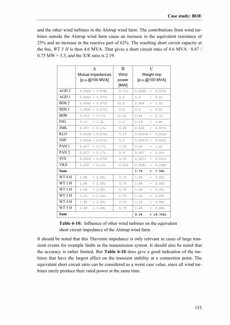
Case study: BOE
153
and the other wind turbines in the Alstrup wind farm. The contributions from wind tur-bines outside the Alstrup wind farm cause an increase in the equivalent resistance of 25% and an increase in the reactive part of 62%. The resulting short circuit capacity at the bus, WT 5 H is then 4.6 MVA. That gives a short circuit ratio of 4.6 MVA · 0.87 / 0.75 MW = 5.3, and the X/R ratio is 2.19.
It should be noted that this Thevenin impedance is only relevant in cases of large tran-sient events for example faults in the transmission system. It should also be noted that the accuracy is rather limited. But Table 6-10 does give a good indication of the tur-bines that have the largest affect on the transient stability at a connection point. The equivalent short circuit ratio can be considered as a worst case value, since all wind tur-bines rarely produce their rated power at the same time.
A Mutual impedances
[p.u.@100 MVA]
B Wind power [MW]
C Weight imp
[p.u.@100 MVA]
AGD 2 0.0064 + 0.078i 0.711 0.0060 + 0.074i AGD 1 0.0063 + 0.077i 0.0 0.0 + 0.0i BDS 2 0.0042 + 0.072i 10.5 0.059 + 1.0i BDS 1 0.0043 + 0.073i 0.0 0.0 + 0.0i BØR 0.053 + 0.17i 12.02 0.84 + 2.7i ING 0.14 + 1.3i 1.0 0.19 + 1.8i JMK 0.057 + 0.17i 0.26 0.020 + 0.057i KLO 0.0018 + 0.070i 0.15 0.00036 + 0.014i NSP 0.0018 + 0.070i 0.3 0.00073 + 0.028i PAN 1 0.057 + 0.17i 7.35 0.56 + 1.6i PAN 2 0.057 + 0.17i 0.9 0.067 + 0.20i SVE 0.0018 + 0.070i 0.55 0.0013 + 0.051i VRÅ 0.030 + 0.13i 0.225 0.0091 + 0.038i Sum 1.76 + 7.58i WT 0 H 1.08 + 2.00i 0.75 1.08 + 2.00i WT 1 H 1.08 + 2.00i 0.75 1.08 + 2.00i WT 2 H 1.08 + 2.00i 0.75 1.08 + 2.00i WT 3 H 1.20 + 2.04i 0.75 1.20 + 2.04i WT 4 H 1.34 + 2.06i 0.75 1.34 + 2.06i WT 5 H 1.49 + 2.08i 0.75 1.49 + 2.08i Sum 9.04 + 19.756i
Table 6-10: Influence of other wind turbines on the equivalent short circuit impedance of the Alstrup wind farm.

Case study: BOE
154
Since no dynamic model of the system is available, no fault simulation has been per-formed, but the short circuit ratio is comparable to the short circuit ratio in the example in section 4.2.2.1, page 63. The equivalent short circuit ratio only takes the other wind turbines into account. It is believed that the CHPs will have a positive or in worst case no effect on the stability if they remain connected during a fault. But the loads could have a negative effect on the transient voltage stability. The high reactive power absorption of the consumers could indicate that asynchronous motors e.g. in pumps, fans or compressors, constitute a large part of the load. Because of lack of detailed information on the mix of consumers, this effect has not been further investigated.
6.7.6 Summary In this section, some problems related to the connection of an actual wind farm have been analyzed. Comparisons have been made between load flow simulations of the en-tire system based on measurements, and relatively simple estimates based on a Theve-nin representation of the rest of the network. It has been shown that for this configura-tion the single bus approach provides a good estimate of the voltage rise at the connec-tion point and the voltage sensitivity at the point of common coupling. It has also been shown that adjacent wind turbines and automatic tap changers dramatically change the equivalent impedances for the calculations. The losses related to the active and reactive power transfer of the wind farm have been estimated. It has been shown that the total load dependent mean losses related to the wind farm make 3 % of the mean power production. As seen in Table 6-8, page 137, the mean load dependent losses allocated to all wind turbines in the system is only 2 % of the produced power. The reason for the difference is that this wind farm is connected through a relatively long radial. The active power losses which are related to the reac-tive power absorption of the no load compensated wind farm is estimated as 0.25 % of the total produced power. The influence of the wind turbines in the rest of the system on the transient stability has been roughly estimated. It was shown that the other wind turbines in the system caused an increase in the equivalent Thevenin resistance of 19 % and an increase in the equiva-lent reactance of 62 %. The short circuit ratio of the whole wind farm is 8.9, but if the influence from other wind turbines in the system is taken into account, it is only 5.5 Due to lack of data for the consumers and generators, the actual influence was not simu-lated, but the method was demonstrated in the example in section 4.2.2.1, page 63. Although a program like PowerFactory® can easily be used for an accurate assessment of the problems that were shown here, the calculation of the equivalent impedances can be used for ranking of different possible connection points of a production unit or when defining the requirements for the generator and the control system.

Case study: BOE
155
6.8 Summary A distribution system with a high penetration of wind power and power from combined heat and power plants has been analyzed. The analysis has been based on a load flow model of the system and 10 months of measurement data. Simulations of approximately 27000 15 minute intervals have been performed, and the simulations have been vali-dated by comparing the simulated flows in the transmission transformers with the meas-ured values. There is some discrepancy between the simulated and the measured reac-tive power, especially when the exchange is close to 0. Based on the available informa-tion, it is not possible to identify the source of the deviations.
6.8.1 Losses The losses of the system have been analyzed using the sensitivity analysis method and the current injection method presented earlier. For the 60 kV system and above, there is a clear synergy effect between production and load. These losses, however, only ac-count for 10 % of the total system losses. For the 10 kV system, it is concluded that the cross effects between load and production make a relatively small part of the total sys-tem losses, because the larger wind farms and CHPs are connected to the 60 / 10 kV stations through their own radials. Based on the regression analysis of feeders with only a few smaller wind turbines and CHPs, it is, however, concluded that some of the smaller units do contribute to lowering the losses. The influence of reactive power trans-fer through the 60/10 kV transformers and above only generates 5 % of the load de-pendent losses.
6.8.2 Reactive power balancing The reactive power exchange with the transmission system must be between 9 MVAr export and 2 MVAr import 98 % of a year. Because measurement data has not been analyzed for a whole year, and because of the deviation between the measured and the simulated reactive power exchange, it cannot be determined, if this requirement is met, but it seems that the biggest problem is the reactive power import. Simplified estimates indicate that the largest benefit of a coordinated control of the power factor of the CHPs and the capacitor battery is that the export of reactive power can be limited. If the CHPs on the other hand were set to provide power factor of 1 at all times, ap-proximately 9 MVAr of additional switchable capacitors would be required to meet the requirement for maximal reactive power import. The current synergy effect between the reactive power production of the CHPs and the reactive power absorption of the loads is caused by the fact that CHPs still follow a pat-tern which is similar to the load pattern. In the future they might start reacting more directly to fluctuations in the spot prices related to for example the forecasted wind power.

Case study: BOE
156
6.8.3 Analysis of an individual wind farm The wind farm Ny Alstrup which is the wind farm, located with the largest electrical distance from the connection to the transmission system, has been further investigated. Analyses of the voltage profile show that at the limit for reactive power injection at the rated power production is approximately zero. That means that the wind turbine could be full load compensated without violating the upper limit for the voltage magnitude. The total load dependent losses, allocated to the wind turbine with the marginal alloca-tion tool comprise 3 % of the mean production, and the losses related to transfer of reac-tive power are estimated to 0.25 %. The short circuit ratio of the wind farm is 8.9, but if the influence of other wind turbines in the distribution system is taken into account, the equivalent short circuit ratio is re-duced to 5.5.
6.8.4 The simulation The simulations are based on real measurements and a realistic model of the system. It has, however, been necessary to make the following simplifications, which affect the accuracy of the simulation results:
• All loads of a given feeder have been scaled equally over the day, based on a base load situation. A better accuracy could be achieved if measurements were available for each radial rather than each distribution transformer.
• The simulations have been based on mean flows, estimated from three sampled values. The variation within one period and aliasing effects are not taken into account.
• The accuracy of the measurements has not been validated. Especially for the transmission transformers there is a dead band around zero active and reactive power flow where the measurements are distorted.
• The load flow model has not been updated since April 24th 2005. Any reconfigu-rations, for example of the coupling of the 10 kV feeders since that time have not been considered.
Despite these simplifications, the case study has given a very good insight in the propor-tions of a real system. The combination of measurements and a simulation model makes it possible to estimate many quantities in the system that would otherwise be difficult to measure. Especially the losses are difficult to measure, because they are small compared to the actual power flows.
6.8.5 The system The distribution system has been selected for the case study, because it has a large pene-tration of distributed generation. Further, the well equipped SCADA system and the availability of a detailed system model have made it possible to do a detailed study. Both the connection point in the 150 kV network and the partly meshed 60 kV network provide high short circuit power. Further, most larger wind farms an CHPs are con-

Case study: BOE
157
nected directly to the low voltage side of the 60 / 10 kV transformer stations through their own radials. Larger problems related to stability, voltage profile and extraordinar-ily high losses have therefore not been identified. The presented analysis methods can, however, also be applied to weaker grids, where these problems are expected to be more significant.


159
7 CONCLUSIONS AND OUTLOOK
The work has been focused on the following three issues related to distribution systems with a high penetration of distributed generation: Loss allocation, stability, and voltage and reactive power control. The theory has been used in a case study based on the dis-tribution system around Brønderslev in Northern Jutland.
7.1 Loss allocation Different methods have been presented for calculation and allocation of active and reac-tive power losses in a power system, and the methods have been illustrated with some simple examples which are reproducible by others. The two existing algorithms for loss allocation, proportional sharing (flow tracing) and marginal loss allocation have been compared, and it is found that the flow tracing algo-rithm is more suitable for analyses of larger transmission systems than distribution sys-tems. A new method for loss allocation based on current injections and the short circuit im-pedances has been presented. The method makes it possible to identify the cross effects between different participants. The method can also separate the losses into a part which is dependent on the mean production / consumption and a part which is dependent on the covariance, i.e. between different consumers and producers. The losses imposed by the covariance of the flows represent the maximal potential saving which can be achieved by changing the production/consumption time patterns while maintaining the mean flows. Like the marginal loss allocation, this method requires the definition of a slack bus, which is not considered a problem in a distribution system. For very large systems, the method will be relatively computationally intensive because of the lack of sparsity in the impedance matrix. But for smaller systems or smaller parts of a system it is can provide a good overview of the interaction between load and production. The current injection method has also been used to formulate a linear regression prob-lem for allocation of losses in a mathematically strict way. Although it is often more convenient to use active and reactive power injections rather than currents, the analysis has demonstrated which approximations this approach depends on.
7.1.1 Application to the Case study of BOE Net The marginal loss allocation method and the current injection method have been used in the case study to allocate the losses. For the 60 kV system, the results from current in-
Conclusions and outlook
160
jection method have been compared to results from the sensitivity analysis, and the two algorithms show identical results. The advantages of the sensitivity analysis are firstly that the algorithm is a part of most power system simulation tools. In PowerFactory® the calculation of loss sensitivities, however, requires an invocation of the sensitivity tool for each bus under consideration. This can be automated, but it extends the total simulation time. Secondly, the interpretation is well suited for e.g. incentive generating price signals, since it directly gives the price of a small change in production / consump-tion. The advantages of the current injection method are firstly that it is based on the reduced impedance matrix, which contains the short circuit impedances. It is possible to make a rough estimate of the cost of transferring power from one place to another just by looking at the reduced impedance matrix. Like the sensitivity analysis, the algorithm requires a load flow calculation per measurement point to determine the current infeeds. PowerFactory® does not directly support the export of the impedance matrix. It is, however, possible that it could get implemented in a future version of the tool. The linear regression method is a simple way of getting an overview of the losses at 10 kV and below. It is, however, not possible to separate the losses related to components in the same feeder with similar load or production time profiles due to the multicollin-earity problem. For the 60 kV system and above, there is a clear synergy effect between production and load. These losses, however, only account for 10 % of the total system losses. For the 10 kV system, it is concluded that the cross effects between load and production make a relatively small part of the total system losses, because the larger wind farms and CHPs are connected to the 60 / 10 kV stations through their own radials. Based on the regres-sion analysis of feeders with only a few smaller wind turbines and CHPs, it is, however, concluded that some of the smaller units do contribute to lowering the losses. The influ-ence of reactive power transfer through the 60/10 kV transformers and above only gen-erates 5 % of the load dependent losses.
7.2 Stability It has been investigated, which factors affect the short term voltage stability in a distri-bution network with distributed generation when it is exposed to a fault in the transmis-sion system. The influence of adjacent Danish concept wind turbines, CHPs, SVCs and STATCOMs on the Thevenin parameters at a connection point has been examined.
7.2.1 The influence of adjacent wind turbines on the network parameters For the adjacent Danish concept turbines, it is concluded that the effect on a given Dan-ish concept wind turbine can be estimated by scaling up the mutual short circuit imped-ances according to the relative traffic of wind power going through them. This finding is considered new.
Conclusions and outlook
161
7.2.2 The influence from synchronous generators The influence of a synchronous generator running at no load can to some extend be compared to the influence of a constant voltage source behind a transient reactance. When the synchronous generator is highly loaded, this approach is still valid, but the rotor angle should be taken into account which causes positive voltage phase jump when a fault occurs, a negative phase jump when the fault is cleared and a smaller con-tribution to the voltage after the fault is cleared.
7.2.3 The influence of STATCOMS and SVCs It is concluded that a STATCOM or an SVC operating in its linear control region has the effect that the Thevenin impedance at the connection point is reduced, the Thevenin voltage goes towards the set point voltage and the equivalent short circuit power is in-creased. These effects are more evident the closer to the connection point the unit is located and the lower the controller droop is. When an SVC reaches its capacity limit, it can be represented as a capacitor. The effect is that the Thevenin impedance and the Thevenin voltage at the connection point are increased, compared to the uncompensated situation. A STATCOM at its capacity limit can be represented as a current source. It will there-fore not affect the Thevenin impedance. In situations where a STATCOM or an SVC is operating at its limit, the equivalent short circuit power including the compensation de-vice is not considered a good measure of the equivalent strength of the network. It is concluded that the specification of a Thevenin impedance and voltage provides more information about the nature of the network in these cases. It has been shown that the calculation of the Thevenin parameters can either be made based on the impedance matrix of the network or using a stationary short circuit calcula-tion tool, provided that it is able to consider current sources and capacitors. It is concluded that a good measure of the transient stability limit of a squirrel cage in-duction generator is the maximal rotor speed where the electrical braking power is higher than the rated mechanical input power. This value can be used to rate different solutions against each other, but not for a direct estimation of the maximal fault clearing time, since the rotor flux dynamics, and the effect of a flexible shaft will also affect the maximal fault clearing time.
7.2.4 Application to the Case study of BOE The model of the distribution system does not contain dynamic models of the generators or the loads, therefore the stability assessment methods have not been tested in the case study. The influence of the wind turbines in the rest of the system on the transient stabil-ity has, however, been roughly estimated by calculating an equivalent short circuit im-pedance for a given wind turbine in a wind farm under consideration of all other wind turbines in the system. The short circuit ratio of the wind farm is 8.9, but if the influence of other wind turbines in the distribution system is taken into account, the equivalent

Conclusions and outlook
162
short circuit ratio is reduced to 5.5. To evaluate the usability of the equivalent short cir-cuit ratio, a dynamic model of the system would be necessary.
7.3 Voltage / VAr control The problem related to voltage rise in the presence of distributed generation has been examined. Simple expressions for approximation of the maximal potential voltage in-crease related to injection of power with a power factor of one have been derived, based on an equivalent short circuit impedance. If the voltage is controlled by an under load tap changing transformer, the equivalent short circuit impedance for calculation of the voltage rise effect is the impedance between the connection point under consideration and the bus where the voltage is controlled. It is concluded that voltage rise only consti-tutes a problem, when the X/R ratio of the equivalent short circuit impedance is below 3. The limit for reactive power transfer, imposed by the upper and lower voltage magni-tude limits have been visualized by plotting the P/Q curves corresponding to the upper and lower voltage magnitude limits in the complex plane. This makes it possible to stu-dy the effect of changing the Thevenin voltage, the short circuit capacity, the X/R ratio and the limits of the voltage magnitude in a geometric way.
7.3.1 Application to the Case study of BOE The reactive power balance of the network has been analyzed, and given the available control resources the strategy for reactive power control seems to be well chosen. It is concluded that a centralized control of the CHP units could reduce the import of reac-tive power, but the main benefit would be that the reactive power export could be lim-ited. The voltage constraints related to injection of active and reactive power have been evaluated for a specific wind farm. It is concluded that the simplified approaches based on the Thevenin representation of the network can be used to estimate the voltage rise problems.
7.4 Further work
7.4.1 General It would be interesting to investigate, how the whole distribution system can be repre-sented as a Thevenin equivalent seen from the transmission system. This could be used to create better aggregated models of the distribution systems for assessment of stability of the transmission system. Another issue is island operation as proposed for example in [112]. When the system frequency of an island is held by a number of CHP units with relatively low inertia con-stants, the problem of over speeding of Danish concept wind turbines may become a different character. Because the CHPs have inertia constants which are comparable to or

Conclusions and outlook
163
lower than the inertia constants of the wind turbines, the slip of the wind turbines will not increase with the same rate as the rotor speed in case of a large perturbation. It would be interesting to investigate the interaction between wind turbines and CHP units in a system running in island operation further.
7.4.2 The model of BOE Net The combination of a detailed model and actual measurements of the BOE distribution system can be used for further investigations related to integration of distributed genera-tion. The model and the simulation data which has been generated during this project are presently being used in the project, “Self-Organising Distributed Control of a Dis-tributed Energy System with a High Penetration of Renewable Energy” at DTU. If the model is going to be used in future research projects, a few modifications could be considered. Firstly, the accuracy of the simulations could be increased by calibration of the online power measurements. There should be agreement between the measured and the simulated power flow through the transmission transformers. If possible, more re-dundant measurements should be logged. To use the model for the study of transient stability, is should be extended to include dynamic models of the wind turbines, CHPs and to some extend, the consumers. The model should also contain the component protection and the system protection equip-ment. It could also be interesting to simulate a hypothetical installation of a new wind farm in the system with state-of-the-art technology. This could be used to evaluate, how such wind turbines interact with existing DG units and consumers. For a study of centralized and distributed control strategies, the communication and control systems should be modeled. It is presently not clear, if PowerFactory® is suit-able for this purpose. When evaluating the losses, maximal loading, voltage magnitudes etc. it is necessary to simulate a large period to evaluate the changes, imposed by an alternative control strat-egy. If a set of representative data point can be specified in such a way that a weighted simulation of the reduced set of data points gives the same extreme values and mean values, it would reduce the simulation time considerably. Some methods based on fuzzy clustering and convex hull analysis are presented in [129].

165
8 REFERENCES
[1] Hansen, A. D. and Hansen, L. H., "Wind turbine concept market penetration over 10 years (1995-2004)," Wind energy, vol. 10, no. 1, pp. 81-87, 2007.
[2] Wistoft, B., Petersen, F., and Hansen, H. M., Elektricitetens Aarhundrede - Dansk elforsynings historie. Bind 1. 1891-1940 Danske Elværkers Forening, 1991.
[3] Wistoft, B., Hansen, H. M., and Petersen, F., Elektricitetens Aarhundrede - Dansk elforsynings historie. Bind 2. 1940-1991 Danske Elværkers Forening, 1992.
[4] Danmarks Energifortider. Hovedbegivenheder på energiområdet - Available at www.ens.dk. 2006. The Danish Energy Authority.
[5] Energy statistics. Available at www.ens.dk. 2005. The Danish Energy Authority.
[6] Jenkins, N., Allan, R., Crossley, P., Kirschen, D., and Strbac, G., Embedded generation Institu-tion of Electrical Engineers, UK, 2000.
[7] Ackermann, T., Andersson, G., and Söder, L., "Distributed generation: a definition," Electric Power Systems Research, vol. 57, no. 3, pp. 195-204, 2001.
[8] Ackermann, T., "Distributed resources and re-regulated electricity markets," Electric Power Systems Research, vol. 77, no. 9, pp. 1148-1159, 2007.
[9] Ackermann, T., Wind Power in Power Systems John Wiley and Sons, 2005.
[10] Decentral kraftvarme i Danmark. Baggrundsrapport - Systemplan 2002. 2002. Elkraft System (now Energinet.dk).
[11] Pepermans, G., Driesen, J., Haeseldonckx, D., Belmans, R., and D'haeseleer, W., "Distributed generation: definition, benefits and issues," Energy Policy, vol. 33, no. 6, pp. 787-798, 2005.
[12] Ackermann, T. and Knyazkin, V. Interaction between distributed generation and the distribution network: operation aspects. Transmission and Distribution Conference and Exhibition 2002: Asia Pacific.IEEE/PES 2, 1357-1362. 2002. Transmission and Distribution Conference and Ex-hibition, IEEE/PES.
[13] Sørensen, P., Morthorst, P. E., Thomsen, K., Nielsen, C., and Hansen, J. C. Wind power plants status and visions. 259-271. 2005. Risø international energy conference.
[14] Technical regulations for thermal power station units of 1.5 MW and above. TF 3.2.3. 2006. Energinet.dk.
[15] Eltra and Elkraft System. Wind Turbines Connected to Grids with Voltages below 100 kV. T.F. 3.2.6. 2004.

References
166
[16] Kristoffersen, J. R. and Christiansen, P., "Horns Rev offshore windfarm: its main controller and remote control system," Wind Engineering, vol. 27, no. 5, pp. 351-359, 2003.
[17] Nordpool web site. www.nordpool.com . 2007.
[18] Holttinen, H., "The Impact of Large Scale Wind Power Production on the Nordic Electricity System." Ph.D. VTT Technical Research Centre of Finland, 2004.
[19] Østergaard, J. and Jensen, K. K. Ny Mvar-ordning. 506. 1-9-2004. DEFU.
[20] Forskrift for dimensionering af reaktiv effekt (Mvar-ordning). ELT2003-44d. 15-8-2003. Eltra.
[21] Caldon, R., Rossetto, F., and Scala, A., "Reactive power control in distribution networks with dispersed generators: a cost based method," Electric Power Systems Research, vol. 64, no. 3, pp. 209-217, 2003.
[22] Morren, J., "Grid support by power electronic converters of Distributed Generation units." Ph.D. Deflt University of Technology, 2006.
[23] Masters, C. L., "Voltage rise: the big issue when connecting embedded generation to long 11 kV overhead lines," Power Engineering Journal, vol. 16, no. 1, pp. 5-12, 2002.
[24] Viawan, F., "Steady State Operation and Control of Power Distribution Systems in the Presence of Distributed Generation." Licentiate of Engineering Chalmers University of Technology, 2006.
[25] Liew, S. N. and Strbac, G., "Maximising penetration of wind generation in existing distribution networks," IEE Proceedings-Generation Transmission and Distribution, vol. 149, no. 3, pp. 256-262, 2002.
[26] Katiraei, F., Abbey, C., and Bahry, R. Analysis of Voltage Regulation Problem for a 25-kV Distribution Network with Distributed Generation. IEEE Power Enginnering Society General Meeting , 18-22. 2006.
[27] Pálsson, M. Þ., Toftevaag, T., Uhlen, K., and Tande, J. O. G. Large-scale Wind Power Integra-tion and Voltage Stability Limits in Regional Networks. 2002. Power Engineering Society Summer Meeting, IEEE.
[28] IEC 61400-21. Measurement and assessment of power quality characteristics of grid connected wind turbines . 2001. IEC.
[29] Rosas, P., "Dynamic Influences of Wind Power on the Power System." Ph.D. Technical Univer-sity of Denmark, 2003.
[30] Thiringer, T., "Power quality measurements performed on a low-voltage grid equipped with two wind turbines," IEEE Transaction on Energy Conversion, vol. 11, no. 3, pp. 601-606, 1996.
[31] Thiringer, T., Petru, T., and Lundberg, S., "Flicker contribution from wind turbine installations," IEEE Transaction on Energy Conversion, vol. 19, no. 1, pp. 157-163, 2004.
[32] Kauhaniemi, K. and Kumpulainen, L. Impact of distributed generation on the protection of dis-tribution networks. 315-318. 2004. Eighth IEE International Conference on Developments in Power System Protection.
[33] Slootweg, J. G. and Kling, W. L. Impacts of Distributed Generation on Power System Transient Stability. 862-867. 2002. Power Engineering Society Summer Meeting, IEEE.
[34] Akhmatov, V., "Analysis of dynamic behaviour of electric power systems with large amount of wind power." Ph.D. Technical University of Denmark, 2003.

References
167
[35] Knazkins, V., "Stability of Power Systems with Large Amounts of Distributed Generation." Ph.D. KTH Electrical Engineering, 2004.
[36] Hoff, T. E., Perez, R., Braun, G., Kuhn, M., and Norris, B. The Value of Distributed Photovol-taics to Austin Energy and the City of Austin. 2006. Austin Energy.
[37] Mendez, V. H., Rivier, J., De La Fuente, J. I., Gomez, T., Arceluz, J., Marin, J., and Madurga, A., "Impact of distributed generation on distribution investment deferral," International Journal of Electrical Power & Energy Systems, vol. 28, no. 4, pp. 244-252, 2006.
[38] Buchholz, B. M., and Styczynski, Z. A. New tasks create new solutions for communication in distribution systems. Power Engineering Society General Meeting, 2006.IEEE , 5. 2006.
[39] IEC 61850: Communications Networks and Systems in Substations, International Standard. 2003. IEC.
[40] IEC 61400-25 Communication for monitoring and control of wind turbines (Draft). 2003. IEC.
[41] Svensson, J., "Active Distributed Power Systems." Ph.D. Dept. of Industrial Electrical Engineer-ing and Automation, Lund University, 2006.
[42] Dortolina, C. A. and Nadira, R., "The loss that is unknown is no loss at all: a top-down/bottom-up approach for estimating distribution losses," IEEE Transactions on Power Systems, vol. 20, no. 2, pp. 1119-1125, 2005.
[43] Lakervi, E. and Holmes, E. J., Electricity distribution network design Peter Peregrinus Ltd, 1995.
[44] DIgSILENT. PowerFactory® user manual. [13.1 Build 260]. 2006.
[45] Glover, J. D. and Sarma, M. S., Power System Analysis and Design Brooks/Cole, 2002.
[46] Conejo, A. J., Galiana, F. D., and Kockar, I., "Z-bus loss allocation," Power Systems, IEEE Transactions on, vol. 16, no. 1, pp. 105-110, 2001.
[47] Costa, P. M. and Matos, M. A., "Loss allocation in distribution networks with embedded genera-tion," IEEE Transactions on Power Systems, vol. 19, no. 1, pp. 384-389, 2004.
[48] Cardell, J. B. Improved Marginal Loss Calculations During Hours of Transmission Congestion. 2005. 38th Annual Hawaii International Conference on System Sciences.
[49] Herter, K., "Residential implementation of critical-peak pricing of electricity," Energy Policy, vol. 35 pp. 2121-2130, 2007.
[50] Conejo, A. J., Arroyo, J. M., Alguacil, N., and Guijarro, A. L., "Transmission loss allocation: a comparison of different practical algorithms," IEEE Transactions on Power Systems, vol. 17, no. 3, pp. 571-576, 2002.
[51] Al-Rajhi, A. N. and Bialek J.W. Marginal and Tracing Pricing of Transmission an Empirical Comparison. 2002. 14th Power Systems Computation Conference.
[52] Mutale, J., Strbac, G., Curcic, S., and Jenkins, N., "Allocation of losses in distribution systems with embedded generation," IEE Proceedings-Generation Transmission and Distribution, vol. 147, no. 1, pp. 7-14, 2000.
[53] Liu, L. and Zobian, A., "The Importance of Marginal Loss Pricing in an RTO Environment," The Electricity Journal, vol. 15, no. 8, pp. 40-45, 2002.
[54] Fangxing Li, Jiuping Pan, and Chao, H. Marginal loss calculation in competitive electrical en-ergy markets. 205-209. 2004. IEEE International Conference on Electric Utility Deregulation, Restructuring and Power Technologies, IEEE.
References
168
[55] DIgSILENT. Sensitivity Analysis for Voltage Stability Evaluation. 2003.
[56] Staniulis, R., Deksnys, R., and Samuelsson, O. Exchange of reactive power between national and regional networks - a comparative case study using PowerWorld. 2002. Nordic and Baltic work-shop on power systems, Tampere.
[57] Söder, L., "Estimation of reduced electrical distribution losses depending on dispersed small scale energy production," Proc 12th PSCC, vol. 2 pp. 1229-1234, 1996.
[58] Bialek J.W., "Tracing the flow of electricity," IEE Proceedings-Generation Transmission and Distribution, vol. 143, no. 4, pp. 313-320, 1996.
[59] Pantoš, M. and Gubina, F., "A flow-tracing method for transmission networks," The Interna-tional Journal on Energy, vol. 30, no. 10, pp. 1781-1792, 2005.
[60] Dai, Y., Liu, X. D., Ni, Y. X., Wen, F. S., Han, Z. X., Shen, C. M., and Wu, F. F., "A cost allo-cation method for reactive power service based on power flow tracing," Electric Power Systems Research, vol. 64, no. 1, pp. 59-65, 2003.
[61] Lund, T., Nielsen, J. E., Hylle, P., Sørensen, P., Nielsen, A. H., and Sørensen, G., "Reactive Power Balance in a Distribution Network with Wind Farms and CHPs," International Journal of Distributed Energy Resources, vol. 3, no. 2, pp. 113-138, 2007.
[62] Hong, Y. Y., Chao, Z. T., and Yang, M. S., "A fuzzy multiple linear regression based loss for-mula in electric distribution systems," Fuzzy Sets and Systems, vol. 142, no. 2, pp. 293-306, 2004.
[63] Hong, Y. Y. and Chao, Z. T., "Development of energy loss formula for distribution systems using FCN algorithm and cluster-wise fuzzy regression," Power Delivery, IEEE Transactions on, vol. 17, no. 3, pp. 794-799, 2002.
[64] Mendenhall, W., Beaver, B. M., and Beaver, R. J., Introduction to Probability and Statistics Thomson Brooks/Cole, 2003.
[65] Draper, N. R. and Smith, H., Applied Regression Analysis, 2. ed. John Wiley & Sons New York, 1981.
[66] Johnson, R. A. and Wichern, D. W., Applied multivariate statistical analysis, 5. ed. Prentice-Hall, Inc. Upper Saddle River, NJ, USA, 2002.
[67] Jobson, J. D., Applied Multivariate Data Analysis Springer-Verlag, 1991.
[68] Lund, T. Measurement based analysis of active and reactive power losses in a distribution net-work with wind farms and CHPs. 2007. European Wind Energy Conference & Exhibition, Mi-lan, EWEA.
[69] Svensson, L. and Lundberg, M. Estimating complex covariance matrices. Thirty-Eighth Asilo-mar Conference on Signals, Systems and Computers , 2151-2154. 2004.
[70] Tender specifications for regulating reserves and ancillary services, technical part. 223752 v2. 2005. Energinet.dk.
[71] Kundur, P., Power System Stability and Control McGraw-Hill. Inc., 1994.
[72] Kundur, P., Paserba, J., Ajjarapu, V., Andersson, G., Bose, A., Cañizares, C. A., Hatziargyriou, N. D., Hill, D., Stankovic, A., Taylor, C. W., Van Cutsem, T., and Vittal, V., "Definition and Classification of Power System Stability," IEEE Transactions on Power Systems, vol. 19, no. 2, pp. 1387-1401, 2004.
[73] Taylor, C. W., Power System Voltage Stability McGraw Hill, 1994.
References
169
[74] Van Cutsem, T. and Vournas, C., Voltage stability of electric power systems Kluwer Academic Publishers, 1998.
[75] DEFU. Tilslutning af vindmøller til lav- og mellemspændingsnettet. Committee report 111. 1998.
[76] Affärsverket svenska kraftnäts föreskrifter och allmänna råd om driftsäkerhetsteknisk ut-formning av produktionsanläggningar. 2005. Stockholm, Svenska Kraftnät.
[77] Grid Code: High and extra high voltage. 2003. E.ON Netz GmbH Bayreuth, Germany.
[78] Grid Code Version 2.0. 2007. Eir Grid, Ireland.
[79] Eltra and Elkraft System. Wind turbines connected to grids with voltages above 100 kV. T.F. 3.2.5. 2004.
[80] Jauch, C., Matevosyan, J. M., Ackermann, T., and Bolik, S. M., "International Comparison of Requirements for Connection of Wind Turbines to Power Systems," Wind energy, vol. 8, no. 3, pp. 295-306, 2005.
[81] Samuelsson, O. and Lindahl, S., "On Speed Stability," IEEE Transactions on Power Systems, vol. 20, no. 2, pp. 1179-1180, 2005.
[82] Akhmatov, V. and Knudsen, H., "An aggregate model of a grid-connected, large-scale, offshore wind farm for power stability investigations - Importance of windmill mechanical system," Elec-trical power and energy systems, vol. 24 pp. 709-717, 2002.
[83] Akhmatov, V., Knudsen, H., Nielsen, A. H., Pedersen, J. K., and Poulsen, N. K., "Modelling and transient stability of large wind farms," International Journal of Electrical Power & Energy Sys-tems, vol. 25, no. 2, pp. 123-144, 2003.
[84] Akhmatov, V. and Knudsen, H., "Large penetration of wind and dispersed generation into Dan-ish power grid," Electric Power Systems Research, vol. 77, no. 9, pp. 1228-1238, 2007.
[85] Akhmatov, V., "System stability of large wind power networks: A Danish study case," Interna-tional Journal of Electrical Power & Energy Systems, vol. 28, no. 1, pp. 48-57, 2006.
[86] Niiranen, J. Voltage dip ride through of a doubly-fed generator equipped with an active crowbar. 2004. Nordic Wind Power Conference Chalmers University of Technology, Göteborg, Sweden.
[87] Eriksen, P. B., Ackermann, T., Abildgaard, H., Smith, P., Winter, W., and Garcia, J. R., "System operation with high wind penetration - The transmission challenges of Denmark, Germany, Spain, and Ireland," Power and Energy Magazine, IEEE, vol. 3, no. 6, pp. 65-74, 2005.
[88] Analyse af udfald af decentrale kraftvarmeværker ved netfejlen den 12. januar 2004. 185874 v2. 2004. Eltra.
[89] Lund, T., Eek, J., Uski, S., and Perdana, A. Dynamic fault simulation of wind turbines using commercial simulation tools. 238-246. 2005. 5. International workshop on large-scale integra-tion of wind power and transmission networks for offshore wind farms, Glasgow.
[90] Eek, J., Lund, T., and Di Marcio, G. Voltage stability issues for a benchmark grid model includ-ing large scale wind power. 2006. Nordic Wind Power Conference, Espoo, Finland.
[91] Hansen, J. R., Elforsyngingssystemer, 2 ed. Technical university of Denmark, 2000.
[92] Pedersen, K. O. H., Nielsen, A. H., and Poulsen, N., "Short-circuit impedance measurement," IEE Proceedings-Generation Transmission and Distribution, vol. 150 pp. 169-174, 2003.

References
170
[93] Timbus, A. V., Rodriguez, P., and Teodorescu, R. Grid impedance identification based on active power variations. 2007. IEEE Industry Applications Conference.
[94] Leonhard, W., Control of Electrical Drives, 2nd ed. Springer, 1997.
[95] Holdsworth, L., Jenkins, N., and Strbac, G. Electrical stability of large, offshore wind farms. Seventh International Conference on AC-DC Power Transmission , 156-161. 2001.
[96] Sørensen, P., Hansen, A. D., Janosi, L., Bech, J., and Bak-Jensen, B. Simulation of Interaction between Wind Farm and Power System. 1281. 2001. Risø National Laboratory.
[97] Kimbark, E. W., Power System Stability: Synchronous Machines John Wiley and Sons, Inc. New York, 1956.
[98] Anderson, P. M. and Fouad, A. A., Power system control and stability (revised printing) IEEE Press, New York, 1994.
[99] Bollen, M. H. J., Olguin, G., and Martins, M., "Voltage Dips at the Terminals of Wind Power Installations," Wind energy, vol. 8, no. 3, pp. 307-318, 2005.
[100] Cañizares, C. A. and Faur, Z. T., "Analysis of SVC and TCSC Controllers in Voltage Collapse," IEEE Transactions on Power Systems, vol. 14, no. 1, pp. 158-165, 1999.
[101] Cañizares, C. A., Corsi, S., and Pozzi, M. Modeling and Implementation of TCR and VSI Based FACTS Controllers. AT-UCR 99/595. 1999. ENEL Ricerca, Area Trasmissione e Dispaccia-mento.
[102] Sørensen, P., Hansen, A. D., Christensen, P., Mieritz, M., Bech, J., Bak-Jensen, B., and Nielsen, H. Simulation and Verification of Transient Events in Large Wind Power Installations. 1331. 2003. Risø National Laboratory.
[103] Thiringer, T., "Measurement and modeling of low-frequency disturbances in induction ma-chines." Ph.D. Chalmers University of Technology, Göteborg, Sweden, 1996.
[104] EN 50160 - Voltage characteristics of electricity supplied by public distribution systems. 1999. European Committee for Electrotechnical Standardization.
[105] Recommendation 16: Spændingskvalitet i lavspændingsnet. 16. 1995. DEFU.
[106] Teknisk Forskrift 5.3.3 Vest Spændings- og Mvar-regulering. 2004. Energinet.dk.
[107] Anlægsplan 2006 for eltransmission i Danmark. 236076. 2005. Energinet.dk.
[108] Nielsen, S. B., Jensen, C. O., Andersen, N., Megos, J., and Claus, M. Dynamic voltage control of offshore Wind Turbines by using a SVC. 137-142. 2006. Sixth International Workshop on Large-Scale Integration of Wind Power and Transmission Networks for Offshore Wind Farms, Delft.
[109] Søbrink, K. H., Power quality improvements of wind farms Eltra, 1998.
[110] Fastlæggelse af MVAr Bånd. Notat ELT2003-213b Dok nr. 191498. 2004. Eltra.
[111] Lund, P., Cherian, S., and Ackermann, T., "A Cell Controller for Autonomous Operation of a 60 kV Distribution Area," International Journal of Distributed Energy Resources, vol. 2, no. 2, pp. 83-100, 2005.
[112] Lund, P. The Danish Cell Project - Part 1: Background and General Approach. 2007. IEEE Power Engineering Society General Meeting Tampa, USA.
[113] Baldick, R., "Reactive issues - Reactive power in restructured markets," Power and Energy Magazine, IEEE, vol. 2, no. 6, pp. 14-17, 2004.

References
171
[114] Tilslutning af regulerkraftanlæg. Rev. 5 document number 15824-07. 2007. Energinet.dk.
[115] Xu, W., Zang, Y., daSilva, L. P. C., and Kundur, P. Competitive Procurement of Dynamic Reac-tive Power Support Service for Transmission Access. 543-548. 2000. Power Engineering Soci-ety Summer Meeting.
[116] Pirayesh, A., Vakilian, M., Feuillet, R., and Hadj-Said, N., "A conceptual structure for value based assessment of dynamic reactive power support in power markets," Electric Power Systems Research, vol. 77, no. 7, pp. 761-770, 2007.
[117] Johnsen, K., "Aspects of Wind Turbines and CHP in a Liberalised Swedish Power System." Ph.D. Section of Electric Power Engineering, Technical University of Denmark, 2007.
[118] Federal Energy Regulatory Commission (FERC). Principles for Efficient and Reliable Reactive Power Supply and Consumption. 2005.
[119] XLPE Cable Systems. User´s guide - Revision. 2 Available at www.abb.com/cables. 2006. ABB.
[120] Lund, T., Sørensen, P., and Eek, J., "Reactive Power Capability of a Wind Turbine with Doubly Fed Induction Generator," Wind energy, vol. 10, no. 4, pp. 379-394, 2007.
[121] Repo, S., Laaksonen, H., Jarventausta, P., Huhtala, O., and Mickelsson, M. A case study of a voltage rise problem due to a large amount of distributed generation on a weak distribution net-work. Power Tech Conference Proceedings, 2003 IEEE Bologna 4. 2003.
[122] Dai, C. and Baghzouz, Y. On the voltage profile of distribution feeders with distributed genera-tion. Power Engineering Society General Meeting, 2003, IEEE 2, 1136-1140. 2003.
[123] Navarro, I. R., "Dynamic Power System Load." Ph.D. Department of Industrial Electrical Engi-neering and Automation - Lund University, 2005.
[124] Welfonder, E., Weber, H., and Hall, B., "Investigations of the frequency and voltage dependence of load partsystems using a digital self-acting measuring and identification system," IEEE Transactions on Power Systems, vol. 4, no. 1, pp. 19-25, 1989.
[125] Price, W. W., Chiang, H. D., Clark, H. K., Concordia, C., Lee, D. C., Hsu, J. C., Ihara, S., King, C. A., Lin, C. J., Mansour, Y., Srinivasan, K., Taylor, C. W., and Vaahedi, E., "Load representa-tion for dynamic performance analysis," IEEE Transactions on Power Systems, vol. 8, no. 2, pp. 472-482, 1993.
[126] Nyfors web page. http://www.nyfors.dk . 2007.
[127] Lov nr. 495 af 9. juni 2004 om ændring af lov om elforsyning og lov om varmeforsyning - (Markedsovergang for miljøvenlig elektricitet, fremme af vindmølleudbygning, anvendelse af brændsler i kraft-varme-værker m.v.). Link available at www.energistyrelsen.dk.
[128] Beregning af Mvar-bånd på 60 kV-siden af 150/60 kV-transformeren. Document nr. 218957 v2. 2005. Energinet.dk.
[129] Pregelj, A., Begovic, M., and Rohatgi, A., "Quantitative techniques for analysis of large data sets in renewable distributed generation," IEEE Transactions on Power Systems, vol. 19, no. 3, pp. 1277-1285, 2004.


173
A LOSS CALCULATIONS
Loss calculation based on current injections This section briefly shows the derivation of (3.12), page 32 (A.1) is the impedance matrix of a system with one slack bus and a number of busses with fixed current injection. All other busses have been removed from the impedance matrix.
⋅
=
I
SL
I
SL
II
ZZZZ
VV
2221
1211 ( A.1)
If the voltage at the slack bus and the currents injections at the other busses are known, the needed current injection of the slack bus can calculated from (A.2)
ISLSL IZZVZI 121
111
11−− −= ( A.2)
Inserting (A.2) in (A.1) gives the expression in (A.3) for the voltage at the busses with constant current injection.
( )
( ) SL21I2122
ISL21I22I
VZZIZZZZ
IZZVZZIZV1
11121
11
121
111
11
−−
−−
⋅+⋅⋅−
=⋅−+⋅= ( A.3)
The variables in (A.4) to (A.6) are defined to simplify the following expressions.
121
11 ZZZZZ 2122I−⋅−= ( A.4)
1−⋅= 112121 ZZK ( A.5)
12111 ZZK 12
−= ( A.6)
The total losses in the system can be expressed as the sum of all power injections, in-cluding the one from the slack bus. This can be expressed as (A.7)
II*SLSLloss VIIVS ⋅+=
H ( A.7)
Inserting (A.2) and (A.3) in (A.7) and substituting with the variables in (A.4) to (A.6) leads to (A.8).
( ) ( )SL21III12SL11SLloss VKIZIIKVZVS ⋅+⋅⋅+⋅−= −I
H*1 ( A.8)
Expanding (A.8) gives (A.9)
( ) IIISL21II12SLSL11SLloss IZIVKIIKVVZVS ⋅+⋅⋅+⋅−= − H****1 ( A.9)
Assuming that the impedance matrix is symmetrical, i.e. no phase shifting transformers are present, (A.9) can be reformulated as (A.10)

Loss calculations
174
( ) ( ) SL21IIIISL11SLloss VKIIZIVZVS ⋅⋅⋅+⋅+= − imag2**1 HH ( A.10)
Marginal loss allocation This section presents a brief derivation of the marginal loss allocation methods referred to in Section 3.2.1 page 35 and 3.2.3. page 36 The fundamental theory is described in [52]. An alternative way of calculating the sensitivities from the branch-node Jacobian matrix is given in [55]. The complex power flows described with (3.1) can be rewritten in terms of voltage an-gles and magnitudes as shown in (A.11) and (A.12).
( )( ) ( )nknkseriesnknknkkseriesnknknk VVBVVVGP δδδδ −−−−= −−≠sincos ,
2,, ( A.11)
( )( ) ( )nknkseriesnknknkkseriesnknknk VVGVVVBQ δδδδ −−−−−= −−≠sincos ,
2,, ( A.12)
Where ( )knseriesnkG Y−ℜ=−,
( )knseriesnkB Y , −ℑ=−
kV∠=kδ
kV=kV
The losses in the series components can be calculated as the sum of the power fed into the element from both ends. Adding Pk,n and Pk,n for all connected bus bars yields (A.13) since the sine elements cancel each other out. (A.14) shows the same calculation for the reactive power.
( )( )[ ]∑∑= =
−− −−+=N
k
N
nnknknkseriesnkseriesloss VVVVGP
1 1
22, cos2
21 δδ ( A.13)
( )( )[ ]∑∑= =
−− −−+−=N
k
N
nnknknkseriesnkseriesloss VVVVBQ
1 1
22, cos2
21 δδ ( A.14)
The shunt losses are given by (A.15) and (A.16)
[ ]∑=
−− =N
kshuntkkshuntloss GVP
1
2 ( A.15)
[ ]∑=
−− −=N
kshuntkkshuntloss BVQ
1
2 ( A.16)
Where
( )∑=
− =N
nshuntkkG
1. real nk,Y
( )∑=
− =N
nshuntkkB
1. imag nk,Y
The partial derivatives of the active and reactive power losses in (A.13) to (A.16) with respect to the angle and magnitude of the bus voltages are given in (A.17) to (A.20).

Loss calculations
175
( )[ ]∑=
− −=∂∂ N
nnknkseriesnk
k
loss VVGP
1, sin2 δδ
δ ( A.17)
( )( )[ ]∑=
−− −−+=∂∂ N
nnknkseriesnkshuntkk
k
loss VVGGVVP
1, cos22 δδ ( A.18)
( )[ ]∑=
− −−=∂∂ N
nnknkseriesnk
k
loss VVBQ
1, sin2 δδ
δ ( A.19)
( )( )[ ]∑=
−− −−−−=∂∂ N
nnknkseriesnkshuntkk
k
loss VVBBVVP
1, cos22 δδ ( A.20)
The partial derivatives of the losses with respect to the active and reactive power injec-tions can be found by solving the linear system in (A.21)
∂∂
∂∂∂∂
∂∂
=
∂∂
∂∂∂∂
∂∂
⋅
N
loss
loss
N
loss
loss
N
loss
loss
N
loss
loss
T
VP
VP
P
P
QP
QPPP
PP
J
M
M
M
M
2
2
2
2
δ
δ
( A.21)
J T is the transposed Jacobian matrix as defined in (A.22). It is assumed that Bus 1 is the slack bus where the loss sensitivity per definition is zero. Therefore the respective rows and columns have been removed. The definition of the partial derivatives in (A.22) can be found in most books about power system analysis – for example [45].
∂∂
∂∂
∂∂
∂∂
∂∂
∂∂
∂∂
∂∂
∂∂
∂∂
∂∂
∂∂
∂∂
∂∂
∂∂
∂∂
=
N
NN
N
NN
NN
N
NN
N
N
NN
VQ
VQQQ
VQ
VQQQ
VP
VPPP
VP
VPPP
J
LL
MOMMOM
LL
LL
MOMMOM
LL
22
2
2
22
2
2
2
2
2
2
2
22
2
2
δδ
δδ
δδ
δδ
( A.22)
Proportional sharing (tracing) This section very briefly presents some of the algorithms, presented in [58] and [59] associated to the method of tracing. A short description can be found in Section 3.2.2 page 36.
Upstream looking algorithm

Loss calculations
176
The basic idea of the upstream looking method is to describe the connection between the generator outputs and the nodal inflows as in (A.23). It is assumed that the network is lossless. There are different approaches of dealing with the losses. In [58] it is pro-posed to insert virtual loads in the middle of each line to represent the losses and [59] proposes to add the losses to new lines added to each of the nodes. PAP uG = ( A.23)
P is a column vector of the total inflow for each of the nodes, where ith element is de-fined in (A.24). Ui is the set of nodes which have a positive active power flow towards Node i.
[ ] GiUj
jii PPPi
+= ∑∈
Ni ,,1L= ( A.24)
uA is the upstream matrix, where element i,j is defined in (A.25).
[ ]
∈−
=
=
otherwise0
for
for 1
ij
ji
iju UjP
Pji
Α ( A.25)
If uA can be inverted, the nodal flows can be expressed in terms of the generator out-
puts using (A.26). Gu PAP 1−= ( A.26) According to the proportional sharing principle, the relative contribution of each genera-tor to the flow in a given line is the same as the relative contribution of the generator to the nodal flow in the node feeding the line this is expressed in (A.27)
[ ]∑=
−
==
N
kGkiku
i
lii
i
lili PA
PP
PPP
P1
1 ( A.27)
The losses in each line can be allocated to the generators proportionally to the flow they are generating or proportionally to the square of the flow to take the non-linearity of the loss function into account. The same way, the contribution of a given generator to a given load can be calculated.
Example Figure A-1 shows a small example of a lossless network to illustrate the algorithms.

Loss calculations
177
(A.28) shows the upstream distribution matrix calculated according to (A.25)
−−
−−
−−
−−−
=
1050/200060/200
01035/1000100/60
070/101000100/40
0001000
0000100
0000010
00035/2535/3560/401
uA ( A.28)
Table A-1 shows how much each of the generators contribute to the loading of each line. If the losses of each line were known, they could be assigned to the generators ac-cording to these numbers.
i
j
k
l
m
n
40
6025
35
40
o
2020
40
30
60
35
35
60
10
10
G
G
Gi
j
k
l
m
n
40
6025
35
40
o
2020
40
30
60
35
35
60
10
10
GG
GG
GG
Figure A-1: Example of small, lossless network. The numbers refer to active power flows in MW

Loss calculations
178
Line Total [MW] Gj [MW] Gk [MW] Gl [MW]
i,m 40 16 14 10
i,n 60 24 21 15
j,i 40 40 0 0
j,o 20 20 0 0
k,i 35 0 35 0
l,i 25 0 0 25
l,n 10 0 0 10
m,o 20 7.78 6.8 5.43
n,m 10 3.43 3 3.57
Table A-1: Contribution of the generators to the line loads

179
B COMPONENT PARAMETERS
Example Section 3.2.3, 3.3.4 and 4.2.2.1
Wind turbine model The wind turbine and the wind turbine step up transformer are similar to the benchmark models used in [89;102].
Vn [kV] R [Ω/km] X [Ω/km] B [µS/km]
65 0.26 0.41 2.98
10.5 0.16 0.038 226
Table B-1: Data of the two power line types in Figure 3-4 page 38
Vp [kV] Vs [kV] Sn [MVA] ex [%] er [%] i0 [%] P0-loss [kW]
165 65 20 12 0.6 0.25 15
65 10.5 10 9.8 0.65 0.4 6.5
Table B-2: Data of the two transformer types in Figure 3-4 page 38
Vp [kV] Vs [kV] Sn [MVA] ex [%] er [%] i0 [%] P0-loss [kW]
10.5 0.96 2.0 6.7 1 0.8 0
Table B-3: Data of the wind turbine transformers
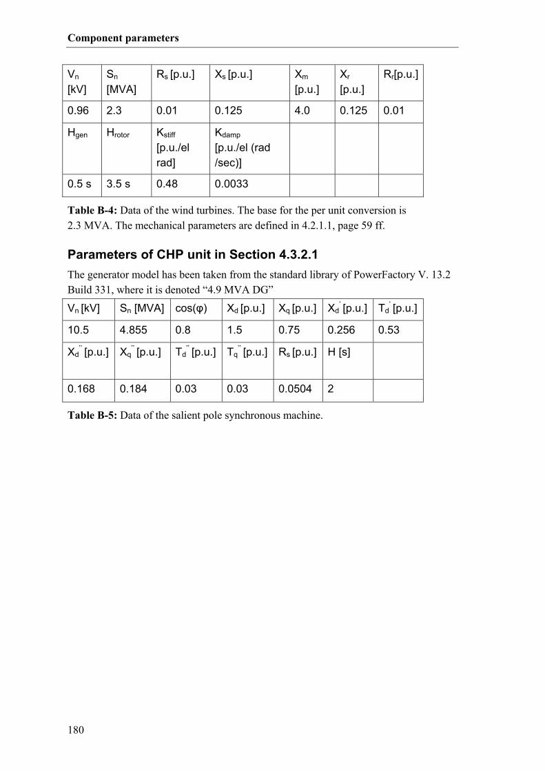
Component parameters
180
Parameters of CHP unit in Section 4.3.2.1 The generator model has been taken from the standard library of PowerFactory V. 13.2 Build 331, where it is denoted “4.9 MVA DG”
Vn
[kV] Sn [MVA]
Rs [p.u.] Xs [p.u.] Xm
[p.u.] Xr
[p.u.] Rr[p.u.]
0.96 2.3 0.01 0.125 4.0 0.125 0.01
Hgen Hrotor Kstiff [p.u./el rad]
Kdamp
[p.u./el (rad /sec)]
0.5 s 3.5 s 0.48 0.0033
Table B-4: Data of the wind turbines. The base for the per unit conversion is 2.3 MVA. The mechanical parameters are defined in 4.2.1.1, page 59 ff.
Vn [kV] Sn [MVA] cos(φ) Xd [p.u.] Xq [p.u.] Xd’ [p.u.] Td
’ [p.u.]
10.5 4.855 0.8 1.5 0.75 0.256 0.53
Xd’’ [p.u.] Xq
’’ [p.u.] Td
’’ [p.u.] Tq
’’ [p.u.] Rs [p.u.] H [s]
0.168 0.184 0.03 0.03 0.0504 2
Table B-5: Data of the salient pole synchronous machine.

181
C NETWORK DATA BOE
Reduced impedance matrix The table below shows the reduced impedance matrix seen from the 10 kV side of all the 60/10 kV transformers. The 10 kV radials are not considered, and the 150 kV con-nection to the transmission system is short circuited. The reduced matrix has been calcu-lated according to (3.8) page 32 in per unit with a rated power of 1000 MVA. The net-work parameters were obtained by printing the transformer and line parameters with a DPL script in PowerFactory®, and importing them into Matlab®. The tap changers of the transformers have been set to their average value during the period of measure-ments.

182
MV
A
1000
IZ
A
GD
_1
AG
D_2
B
DS
_2
BD
S_1
B
OE
R
ING
JM
K
KLO
N
SP
P
AN
_2
PA
N_1
S
VE
V
RA
A
AG
D_2
0.
4245
1
7.69
82i
0.10
967
0.
8414
5i
0.06
6426
0.
7531
1i
0.06
7462
0.
7647
2i
0.04
8025
0.
7557
5i
0.06
3731
0.
7785
9i
0.07
8987
0.
8044
1i
0.01
7816
0.
7014
9i
0.01
7743
0.
7005
7i
0.07
9248
0.
8072
4i
0.07
9074
0.
8054
8i
0.01
7857
0.
7034
2i
0.03
49
0.73
754i
AG
D_1
0.
1096
7
0.84
145i
0.
8224
7
11.6
01i
0.06
6056
0.
7489
4i
0.06
7086
0.
7604
9i
0.04
7758
0.
7515
7i
0.06
3377
0.
7742
8i
0.07
8549
0.
7999
6i
0.01
7716
0.
6976
1i
0.01
7643
0.
6966
9i
0.07
8809
0.
8027
8i
0.07
8635
0.
8010
2i
0.01
7756
0.
6995
2i
0.03
4706
0.
7334
6i
BD
S_2
0.
0664
26
0.75
311i
0.
0660
56
0.74
894i
0.
2416
5.
1043
i 0.
0754
6
0.75
98i
0.03
3829
0.
7144
7i
0.04
2262
0.
7228
2i
0.05
049
0.
7344
5i
0.01
7442
0.
6882
7i
0.01
7371
0.
6873
7i
0.05
0652
0.
7370
4i
0.05
054
0.
7354
3i
0.01
7482
0.
6901
6i
0.02
6755
0.
7087
2i
BD
S_1
0.
0674
62
0.76
472i
0.
0670
86
0.76
049i
0.
0754
6
0.75
98i
0.45
398
7.
5105
i 0.
0343
59
0.72
548i
0.
0429
23
0.73
397i
0.
0512
78
0.74
578i
0.
0177
18
0.69
888i
0.
0176
45
0.69
796i
0.
0514
43
0.74
84i
0.05
133
0.
7467
7i
0.01
7758
0.
7008
i 0.
0271
75
0.71
965i
BO
ER
0.
0480
25
0.75
575i
0.
0477
58
0.75
157i
0.
0338
29
0.71
447i
0.
0343
59
0.72
548i
0.
9591
6
6.86
82i
0.52
722
1.
6875
i 0.
3819
1.
3336
i 0.
0181
21
0.70
176i
0.
0180
48
0.70
083i
0.
3832
1
1.33
83i
0.38
237
1.
3354
i 0.
0181
63
0.70
368i
0.
3918
4
1.46
i
ING
0.
0637
31
0.77
859i
0.
0633
77
0.77
428i
0.
0422
62
0.72
282i
0.
0429
23
0.73
397i
0.
5272
2
1.68
75i
1.42
94
13.2
62i
0.57
28
1.65
74i
0.01
8206
0.
6989
9i
0.01
8133
0.
6980
7i
0.57
478
1.
6633
i 0.
5735
3
1.65
96i
0.01
8248
0.
7009
1i
0.30
425
1.
2505
i
JMK
0.07
8987
0.
8044
1i
0.07
8549
0.
7999
6i
0.05
049
0.
7344
5i
0.05
1278
0.
7457
8i
0.38
19
1.33
36i
0.57
28
1.65
74i
1.18
78
8.72
51i
0.01
8348
0.
6998
1i
0.01
8274
0.
6988
9i
0.76
016
1.
9838
i 0.
7585
1.
9795
i 0.
0183
9
0.70
173i
0.
2224
1.
0555
i
KLO
0.
0178
16
0.70
149i
0.
0177
16
0.69
761i
0.
0174
42
0.68
827i
0.
0177
18
0.69
888i
0.
0181
21
0.70
176i
0.
0182
06
0.69
899i
0.
0183
48
0.69
981i
1.
5788
13
.735
i 0.
0175
74
0.69
596i
0.
0183
97
0.70
227i
0.
0183
56
0.70
073i
0.
5001
2
1.73
19i
0.01
8062
0.
7056
6i
NS
P
0.01
7743
0.
7005
7i
0.01
7643
0.
6966
9i
0.01
7371
0.
6873
7i
0.01
7645
0.
6979
6i
0.01
8048
0.
7008
3i
0.01
8133
0.
6980
7i
0.01
8274
0.
6988
9i
0.01
7574
0.
6959
6i
0.37
425
7.
2635
i 0.
0183
23
0.70
134i
0.
0182
82
0.69
981i
0.
0176
13
0.69
787i
0.
0179
88
0.70
473i
PA
N_2
0.
0792
48
0.80
724i
0.
0788
09
0.80
278i
0.
0506
52
0.73
704i
0.
0514
43
0.74
84i
0.38
321
1.
3383
i 0.
5747
8
1.66
33i
0.76
016
1.
9838
i 0.
0183
97
0.70
227i
0.
0183
23
0.70
134i
1.
4544
13
.164
i 0.
7611
2
1.98
65i
0.01
8439
0.
7042
i 0.
2231
6
1.05
92i
PA
N_1
0.
0790
74
0.80
548i
0.
0786
35
0.80
102i
0.
0505
4
0.73
543i
0.
0513
3
0.74
677i
0.
3823
7
1.33
54i
0.57
353
1.
6596
i 0.
7585
1.
9795
i 0.
0183
56
0.70
073i
0.
0182
82
0.69
981i
0.
7611
2
1.98
65i
1.39
18
12.9
39i
0.01
8398
0.
7026
6i
0.22
267
1.
0569
i
SVE
0.01
7857
0.
7034
2i
0.01
7756
0.
6995
2i
0.01
7482
0.
6901
6i
0.01
7758
0.
7008
i 0.
0181
63
0.70
368i
0.
0182
48
0.70
091i
0.
0183
9
0.70
173i
0.
5001
2
1.73
19i
0.01
7613
0.
6978
7i
0.01
8439
0.
7042
i 0.
0183
98
0.70
266i
1.
1815
12
.393
i 0.
0181
03
0.70
76i
VR
AA
0.
0349
0.
7375
4i
0.03
4706
0.
7334
6i
0.02
6755
0.
7087
2i
0.02
7175
0.
7196
5i
0.39
184
1.
46i
0.30
425
1.
2505
i 0.
2224
1.
0555
i 0.
0180
62
0.70
566i
0.
0179
88
0.70
473i
0.
2231
6
1.05
92i
0.22
267
1.
0569
i 0.
0181
03
0.70
76i
0.95
654
8.
3945
i

183

www.oersted.dtu.dk/cet Ørsted·DTU Centre for Electric Technology (CET) Technical University of Denmark Elektrovej 325 DK-2800 Kgs. Lyngby Denmark Tel: (+45) 45 25 35 00 Fax: (+45) 45 88 61 11 E-mail: [email protected]