(SYB) 35-1

Analysis of Combined Convective and Film Coolingon an Existing Turbine Blade

Wim B. de WolfNational Aerospace Laboratory

P.O. Box 1538300 AD Emmeloord

The Netherlands

Sandor Woldendorp and Tiedo TingaNational Aerospace Laboratory

P.O. Box 905021006 DM Amsterdam

The Netherlands

Summary

To support gas turbine operators, NLR is developing capabilities for life assessment of hot engine components.As a typical example the first rotor blades of the high pressure (HP) turbine of the F-100-PW-220 militaryturbofan will be discussed. For these blades tools have been developed to derive the blade temperature historyfrom flight data obtained from F-16 missions. The resulting relative life consumption estimate should supportthe Royal Netherlands Air Force in their engine maintenance activities.

The present paper describes the prediction method for the blade temperature, based on reverse engineering.Input data are the flight data of the engine performance parameters and the geometry of the HP turbine bladesand vanes including film cooling orifices. The engine performance parameters are converted in HP turbine entryand exit conditions by the NLR Gas Turbine Simulation Program (GSP) engine model. Next a ComputationalFluid dynamics (CFD) tool is used to calculate the resulting flow field and heat transfer coefficients without filmcooling. An engineering method is used to predict the internal cooling and the resulting film injectiontemperature. The film cooling efficiency is estimated and a finite element method (FEM) for heat conductioncompletes the analysis tool. The method is illustrated by results obtained for the engine design point.

1. Introduction

Gas turbine operators increasingly recognise that the actual lives of gas turbine hot section components often donot reach the predictions. Consequently, there is a greater demand for residual life assessments incorporatingoperational gas turbine parameters and conditions. To respond to this demand, the National AerospaceLaboratory NLR of the Netherlands has developed activities and capabilities to assess lives of gas turbinecomponents.

To develop a life prediction model five main disciplines have to be integrated (see Fig.1). These disciplines areapplied as follows for a turbine blade:- Engine System Performance Analysis, to determine the operational conditions of the turbine (entry

pressure, temperature, mass flow, rpm) from engine performance history data.- Fluid Dynamic Analysis, to determine the thermal and mechanical loads on a turbine blade depending on

the operational conditions of the turbine.- Thermal Analysis, to calculate the temperature distribution in the blade material.- Stress Analysis, to calculate the thermal and mechanical stresses in the blade material.- Life Consumption Assessment, in particular by fatigue, creep and oxidation.

The analysis tool developed by NLR enables gas turbine operators to optimise their inspection intervals,maintenance planning, component replacement and consequently their costs.

To develop an integrated engine design tool with the disciplines involved would require a massive effort thatwould by far exceed the resources at NLR. An analysis tool can however be based upon reverse engineeringusing experience with existing engines. The present paper will illustrate such an approach taking the film cooled

Paper presented at the RTO AVT Symposium on “Advanced Flow Management: Part B – Heat Transfer andCooling in Propulsion and Power Systems”, held in Loen, Norway, 7-11 May 2001, and published in RTO-MP-069(I).

Report Documentation Page Form ApprovedOMB No. 0704-0188

Public reporting burden for the collection of information is estimated to average 1 hour per response, including the time for reviewing instructions, searching existing data sources, gathering andmaintaining the data needed, and completing and reviewing the collection of information. Send comments regarding this burden estimate or any other aspect of this collection of information,including suggestions for reducing this burden, to Washington Headquarters Services, Directorate for Information Operations and Reports, 1215 Jefferson Davis Highway, Suite 1204, ArlingtonVA 22202-4302. Respondents should be aware that notwithstanding any other provision of law, no person shall be subject to a penalty for failing to comply with a collection of information if itdoes not display a currently valid OMB control number.

1. REPORT DATE 00 MAR 2003

2. REPORT TYPE N/A

3. DATES COVERED -

4. TITLE AND SUBTITLE Analysis of Combined Convective and Film Cooling on an ExistingTurbine Blade

5a. CONTRACT NUMBER

5b. GRANT NUMBER

5c. PROGRAM ELEMENT NUMBER

6. AUTHOR(S) 5d. PROJECT NUMBER

5e. TASK NUMBER

5f. WORK UNIT NUMBER

7. PERFORMING ORGANIZATION NAME(S) AND ADDRESS(ES) NATO Research and Technology Organisation BP 25, 7 Rue Ancelle,F-92201 Neuilly-Sue-Seine Cedex, France

8. PERFORMING ORGANIZATIONREPORT NUMBER

9. SPONSORING/MONITORING AGENCY NAME(S) AND ADDRESS(ES) 10. SPONSOR/MONITOR’S ACRONYM(S)

11. SPONSOR/MONITOR’S REPORT NUMBER(S)

12. DISTRIBUTION/AVAILABILITY STATEMENT Approved for public release, distribution unlimited

13. SUPPLEMENTARY NOTES Also see ADM001490, presented at RTO Applied Vehicle Technology Panel (AVT)Symposium held inLeon, Norway on 7-11 May 2001, The original document contains color images.

14. ABSTRACT

15. SUBJECT TERMS

16. SECURITY CLASSIFICATION OF: 17. LIMITATION OF ABSTRACT

UU

18. NUMBEROF PAGES

18

19a. NAME OFRESPONSIBLE PERSON

a. REPORT unclassified

b. ABSTRACT unclassified

c. THIS PAGE unclassified

Standard Form 298 (Rev. 8-98) Prescribed by ANSI Std Z39-18

(SYB) 35-2

rotor blades of the high-pressure turbine of the Pratt and Whitney F100-PW-220 military turbofan engine as anexample. This engine is used by the Royal Netherlands Air Force in their F-16 fighter aircraft.

The variation of the low-pressure turbine entry temperature (FTIT) measured during a typical F-16 mission isshown in figure 2. At take-off FTIT increases from 450 °C (taxi) to 960 °C at full power. At the cruise altitudebetween 37 and 45 kft FTIT varies between 680 °C and 940 °C. During the descent strong temperaturevariations occur as a result of frequent changes in power setting.

The present paper will discuss a method to relate the engine operational conditions to the blade temperature ofthe first stage rotor of the high pressure turbine. The method combines the results from available software toolsto predict the engine thermodynamic performance (the NLR Gas Turbine Simulation Program GSP) and theblade aerodynamics (Numeca’s FINE/Turbo CFD code available at NLR) with engineering estimates of theinternal heat transfer and the film cooling efficiency.

The results may be used to address a number of questions such as: what is the blade failure mode (by creep orfatigue or a combination) and what parts of the mission (and what corresponding power variations) are most lifeconsuming? Finally, a relative or even absolute life consumption estimate can be established to support theengine maintenance activities.

Thermal analysis, stress analysis and the resulting life assessment will not be addressed here but in a future RTOpaper.

2. Approach to predict the blade material temperature

The only information available is the blade geometry and the history of the turbine entry and exit conditions.These conditions are available from recorded flight data, combined with a thermodynamic model of the engineto be discussed later. From this information a realistic estimate should be made of the blade temperature andstress history.

The heat transfer calculations are complicated by the fact that the blades are film cooled by high pressure airfrom the compressor bleed. This air is heated inside the blade before being ejected at a temperature Tinj throughcooling orifices into the outer flow to provide a cooling air layer with effective temperature Tfilm between theblade surface with temperature Tw,ext and the outer hot gas flow.

The external heat transfer qext (W/m2) in the case of film cooling can be expressed as ( Ref.1):

qext = hext (Tfilm − Tw,ext)

It is a well accepted engineering approach to assume that the value of the heat transfer coefficient hext is notaffected by the presence of blade film cooling (Ref.1). In that case hext values can be calculated by wellestablished CFD methods for zero film cooling.

As a result of the discrete point injection and the mixing with the outer flow Tfilm is somewhere between theadiabatic wall temperature without film cooling and Tinj. This is expressed by the film cooling efficiency:

injgas

filmgasfilm TT

TT

−−

=η

Here Tgas is the adiabatic wall temperature without film cooling or, in the case of multiple orifice rows Tgas =Tfilm just upstream of the orifice row (Ref.2). Orifice diameters on the blades considered here are of the order of0.3 mm and orifice rows are typically 6 mm apart. The film cooling efficiency will depend on the streamwisedistance behind the orifice row and on the lateral (spanwise) distance (Ref.1). As a first simplification, a lateralaverage may be used. Typical values are of the order of 0.2 close to the orifice row decreasing to 0.1 at 50orifice diameters downstream (see for instance Ref.1, 3).

A further simplification is to replace the orifice row by a narrow slot of width w with the same cooling air massflow. FINE/Turbo was recently extended with such a slot film cooling model but during its application a numberof practical problems were encountered:• The cooling slots have a width equal to the local grid cell length that was about 5 percent of the blade chord

in the mid-chord region. Film temperatures tend to decrease 2 grid cells ahead of the slot due to numerical

(SYB) 35-3

diffusion. Smaller grids are required for sufficient resolution but have not been used to avoid unacceptablelong computation times.

• The slot cooling model will provide cooling efficiencies that are significantly higher than for orifice coolingnear to the orifice rows. This could be compensated for by choosing a higher injection temperature than forthe orifice cooling.

FINE/Turbo was therefore used to calculate hext without film cooling to be used for the calculations with filmcooling. The option of slot film cooling was used only to improve the prediction of the pressure distribution.

To calculate the external heat transfer, also the film temperature must be determined. This requires a realisticestimate of the film cooling efficiency. In combination with a prediction for the internal heat transfer the bladetemperature distribution can be calculated in an iterative procedure with a Finite Element Method (FEM) modelof the blade, starting with an assumed blade temperature distribution. It is noted that the injection temperaturefollows from the internal heat transfer to the cooling air but in turn the injection temperature affects the filmtemperature and hence the external heat transfer and thus the blade temperature and thus the heating of thecooling air etc., resulting in an iterative procedure.

For the internal cooling an engineering model based on fully developed pipe flow has been used taking intoaccount the effect of turbulators that increase friction losses and heat transfer. Some of the cooling ducts haveorifices that provide the external film cooling. Pressure losses and heat transfer in the orifices can be taken intoaccount again by an engineering prediction.

For calculation of the temperature and the heat conduction in the blade material the computer programs MARCor B2000 are available based on finite element methods.

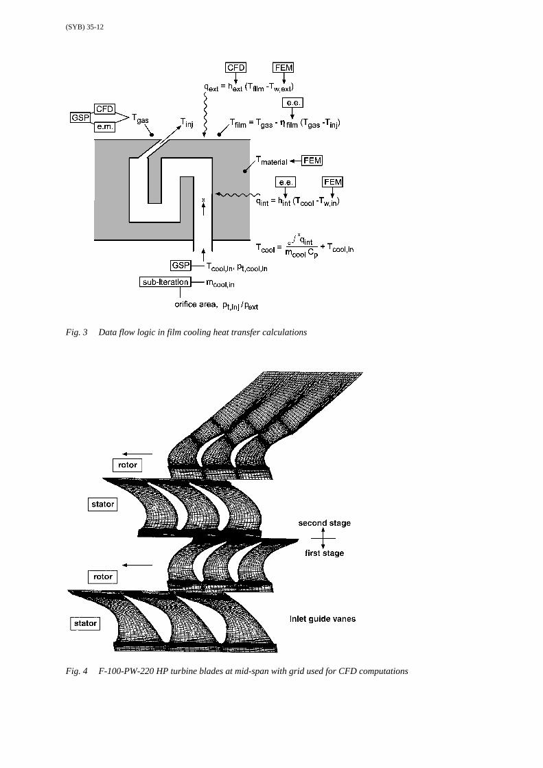
Figure 3 summarises the approach that will be used, depicting the data flow logic. Data processors are indicatedin rectangles. Here ‘e.m.’ stands for engineering methods that are well established and ‘e.e.’ for engineeringestimates. These estimates constitute the weakest elements in the method and should be varied in a sensitivityanalysis. The estimates relate to (i) the influence of the turbulators and centrifugal forces on internal heattransfer in the serpentine cooling ducts and (ii) to the film cooling efficiency. The next chapters will discuss thisapproach and some results in more detail.

3. From flight data to turbine entry and exit conditions.

For assessment of the blade life, the blade temperature history and the resulting stresses must be known. Theengine operational data obtained during a particular flight mission form the starting point.

F-16 fighter aircraft of the RNLAF are being equipped with a fatigue analysis system developed by NLR,combined with the Autonomous Combat Evaluation (ACE) system to form the FACE system. Presently morethan 100 aircraft have an operational FACE system. The relevant signals stored by the FACE Data RecordingUnit are engine parameters from the Digital Electronic Engine Control (DEEC) and avionics data. Thefollowing relevant data are stored: fuel flow to the core engine, fuel flow to the afterburner, exhaust nozzleposition (area) and for the flight conditions: Mach, pressure altitude and air temperature. The DEEC signals canbe sampled at a maximum frequency of 4 Hz.

These data are used as input data for the Gas Turbine Simulation Program (GSP). This is a tool for gas turbineperformance analysis, developed at NLR (Ref.4). This program enables both steady state and transientsimulations for any kind of gas turbine configuration. The simulation is based on one-dimensional modelling ofthe processes in the various gas turbine components with thermodynamic relations and steady-statecharacteristics (component maps). For the F100-PW-220 engine the component maps are based on informationfrom the manufacturer, literature data, and test bench data using reverse engineering. Real gas effects areincluded as well as thermal and mechanical inertia that are important to accurately describe the enginetransients.

For the current application, GSP is used to calculate the high-pressure turbine entry (station 4) and exit (station45) total temperature, total pressure and mass flows including the cooling air supplied to the HP turbine. Thefuel flows and nozzle position input data are replaced by the Power Lever Angle (PLA) signal, as obtained fromFACE. GSP contains a model of the F100-PW-220 engine control unit, which translates the PLA to theappropriate fuel flows and nozzle area. With the engine geometry data also the flow velocities at station 4 and45 can be calculated, assuming a uniform pressure and temperature.

For the high pressure turbine at the engine design point the following data are given below as obtained fromGSP. The design point corresponds to military thrust at static sea level ISA conditions.

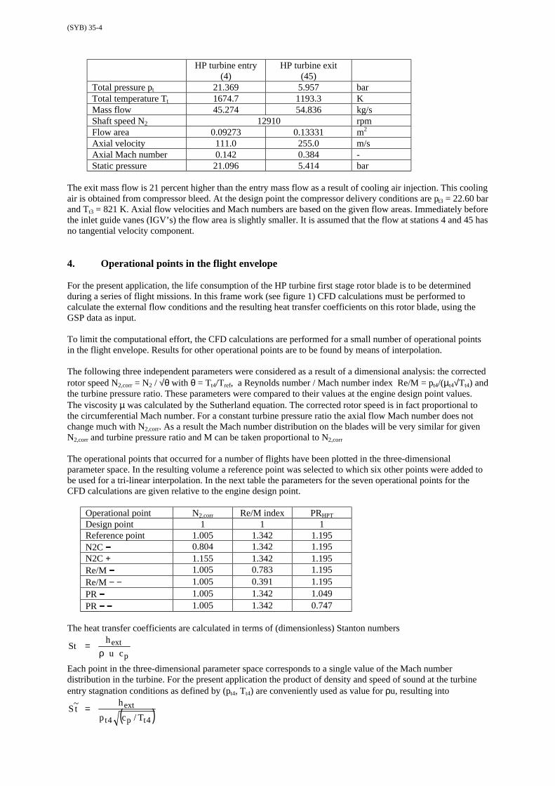
(SYB) 35-4

HP turbine entry(4)

HP turbine exit(45)

Total pressure pt 21.369 5.957 barTotal temperature Tt 1674.7 1193.3 KMass flow 45.274 54.836 kg/sShaft speed N2 12910 rpmFlow area 0.09273 0.13331 m2

Axial velocity 111.0 255.0 m/sAxial Mach number 0.142 0.384 -Static pressure 21.096 5.414 bar

The exit mass flow is 21 percent higher than the entry mass flow as a result of cooling air injection. This coolingair is obtained from compressor bleed. At the design point the compressor delivery conditions are pt3 = 22.60 barand Tt3 = 821 K. Axial flow velocities and Mach numbers are based on the given flow areas. Immediately beforethe inlet guide vanes (IGV’s) the flow area is slightly smaller. It is assumed that the flow at stations 4 and 45 hasno tangential velocity component.

4. Operational points in the flight envelope

For the present application, the life consumption of the HP turbine first stage rotor blade is to be determinedduring a series of flight missions. In this frame work (see figure 1) CFD calculations must be performed tocalculate the external flow conditions and the resulting heat transfer coefficients on this rotor blade, using theGSP data as input.

To limit the computational effort, the CFD calculations are performed for a small number of operational pointsin the flight envelope. Results for other operational points are to be found by means of interpolation.

The following three independent parameters were considered as a result of a dimensional analysis: the correctedrotor speed N2,corr = N2 / √θ with θ = Tt4/Tref, a Reynolds number / Mach number index Re/M = pt4/(µt4√Tt4) andthe turbine pressure ratio. These parameters were compared to their values at the engine design point values.The viscosity µ was calculated by the Sutherland equation. The corrected rotor speed is in fact proportional tothe circumferential Mach number. For a constant turbine pressure ratio the axial flow Mach number does notchange much with N2,corr. As a result the Mach number distribution on the blades will be very similar for givenN2,corr and turbine pressure ratio and M can be taken proportional to N2,corr

The operational points that occurred for a number of flights have been plotted in the three-dimensionalparameter space. In the resulting volume a reference point was selected to which six other points were added tobe used for a tri-linear interpolation. In the next table the parameters for the seven operational points for theCFD calculations are given relative to the engine design point.

Operational point N2,corr Re/M index PRHPT

Design point 1 1 1Reference point 1.005 1.342 1.195N2C −−−− 0.804 1.342 1.195N2C + 1.155 1.342 1.195Re/M −−−− 1.005 0.783 1.195Re/M − − 1.005 0.391 1.195PR −−−− 1.005 1.342 1.049PR −−−− −−−− 1.005 1.342 0.747

The heat transfer coefficients are calculated in terms of (dimensionless) Stanton numbers

p

extcu

hSt

ρ=

Each point in the three-dimensional parameter space corresponds to a single value of the Mach numberdistribution in the turbine. For the present application the product of density and speed of sound at the turbineentry stagnation conditions as defined by (pt4, Tt4) are conveniently used as value for ρu, resulting into

( )4tp4t

ext

T/cp

ht~

S =

(SYB) 35-5

5. The cooling air mass flow distribution in the high-pressure turbine

To predict the effect of mass flow addition by cooling air in the turbine, the distribution of the cooling air in thevarious stages must be determined, the total amount being given by GSP.

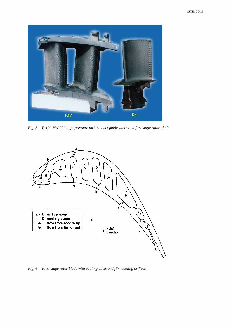
Figure 4 shows the computational grid of the stator and rotor blade sections of the high-pressure turbine near themid-span radius (r = 0.28 m). This grid is used for the CFD calculations. The tapered inlet guide vanes have achord length of 49 mm. The first stage rotor blades are about 46 mm long and have a nearly constant chord of 35mm. As shown in figure 5, the IGV’s and the rotor blades of the first stage have an extensive coverage of filmcooling orifices, in particular near the leading edge, the full pressure side and the forward part of the suctionside. To enhance the film coverage, the orifices near the leading edge are oriented towards the spanwisedirection. The second stage vanes and blades have no film cooling but only internal air cooling. Except for thesecond stage rotor blades, the trailing edges are cooled by air blown from slots at the pressure side a few mmupstream of the trailing edge.

The cooling air distribution was estimated by measuring and counting the film cooling orifices on sample vanesand blades. Orifice diameters varied between 0.25 and 0.4 mm. Measurement accuracy was 0.05 mm. Theeffective orifice area was taken as 80 percent of the geometric area which is a realistic value for pressure ratiospt,cool/pext ≈ 2 (choked orifice flow) with external cross flow (Ref.5). Considering the external pressures on thevarious blades and vanes, an average orifice flow Mach number 0.4 was chosen for the inlet guide vanes, 0.6 forthe first stage rotor blades and for the other blades sonic orifice flow was assumed. Average total pressures andtemperatures just upstream of the orifices had to be estimated, taking into account internal pressure losses andheat transfer. The result is shown in the next table, using γ = 4/3 for the specific heat ratio.

eff orifarea per

blade

numberof blades

total efforif area

pt,cool Tt,cool Minj CoolingMassFlow

percmassflow

mm2 mm2 bar K kg/s %IGV 63.4 44 2790 21.6 1000 0.4 4.79 49.51st R 13.6 68 924 19.2 900 0.6 2.00 20.72nd V 16.0 58 928 20 900 1 2.49 25.82nd R 2.5 72 146 20 900 1 0.39 4.0

all vanes and blades 9.67 100all vanes and blades according to GSP 9.57

In view of the accuracy of the orifice dimensions and the assumptions made, the close agreement with thecooling air mass flow provided by GSP is somewhat fortuitous. At off-design conditions the GSP cooling airmass flows can be used while maintaining the percentage mass flow distribution as shown in the last column.

6. Description of the first stage rotor blade cooling.

Details of the cooling air ducts in first stage rotor blades are shown in figures 6. In fact two cooling air circuitsexist with a common supply at the blade root. The front circuit serves the cooling of the forward 20 percent ofthe blade. The cooling air enters duct 2, separated from the front duct 1 by a perforated wall. Duct 1 containsfive orifice rows (b – f) that provide film cooling to the leading edge. The air jets from the perforations in thewall between duct 1 and 2 provide a mix of internal impingement cooling and enhancement of the turbulencelevel and therewith the heat transfer in duct 1. Orifice rows c-e provide showerhead film cooling of the bladeleading edge near the stagnation point with spanwise orientation rather than streamwise orientation of theorifices to improve film coverage.

The rear cooling circuit starts with duct 7 from where part of the cooling air is passing to parallel ducts 8 and 9.Ducts 7 and 8 have each a row of cooling orifices i and j respectively) and cooling air in duct 9 passes through aslot (k) slightly ahead of the trailing edge to cool the trailing edge at the pressure side. Between ducts 7, 8 and 9the turbulence level is enhanced by the openings between these ducts resembling a pin cooling configuration.

The remaining cooling air at the end of duct 7 near the blade tip returns its direction and passes the serpentinecooling ducts 6 - 3 where duct 5 has a row of cooling orifices at the pressure side of the airfoil (row h) and duct3 has a row of orifices at the pressure side (row g) as well at the suction side (row a). The serpentine coolingduct walls have small strips at 2.5 mm intervals perpendicular to the flow that increase the turbulence level andas a result the internal heat transfer.

(SYB) 35-6

Each of these cooling principles has been studied and described in detail in the literature and their performancecould in principle be calculated by extensive CFD calculations. This was not considered a viable approach sincegrid sizes of the order of say 0.1 mm would be required to model the flow near the cooling orifices. Also theinternal cooling in the serpentine cooling ducts subjected to strong Coriolis forces and turbulators is difficult tomodel. For these aspects engineering predictions are applied instead.

7. Aerodynamic calculations

Aerodynamic calculations of the flow conditions in the high pressure turbine have been performed with theFINE/Turbo code (Ref.6). This CFD model solves the Reynolds-averaged Navier-Stokes equations,complemented with a classical algebraic turbulence model (Baldwin-Lomax). Between the blade rows the ‘exit’flow conditions are circumferentially averaged to be used as ‘entry’ conditions for the next blade row afterchanging from a rotating to a non-rotating system of axes or vice versa. Film cooling is implemented in the formof slot cooling where the cooling orifices are replaced by narrow slots that run in spanwise direction. Cooling airmass flows are duplicated. The slot width winj is chosen equal to the local grid cell length.

Using the computational grid as shown in figure 4 with approximately 621,000 grid nodes, calculations weremade on the complete turbine with respect to aerodynamics and on the first stage rotor blade also on heattransfer (see section 8) on a limited number of operational points. Each operational point required about 16hours of computation time using a single processor ‘SGI Octane’ work station.

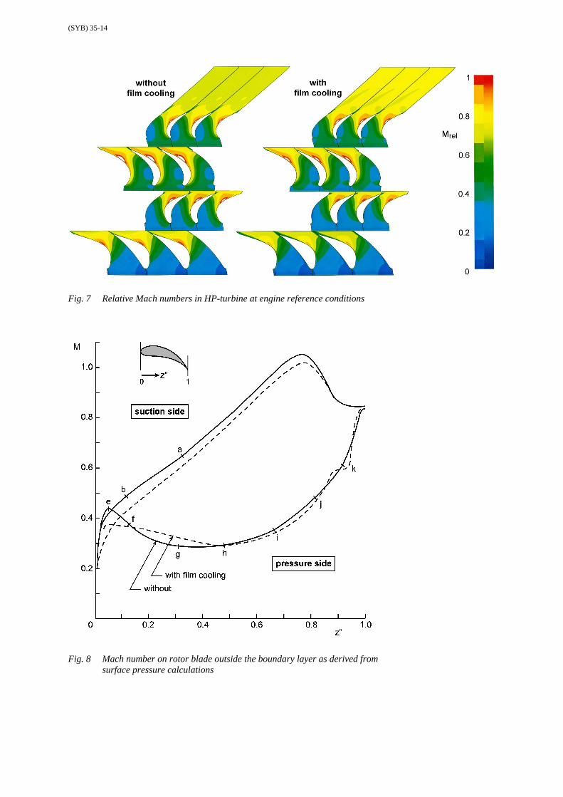
Figure 7 shows the resulting Mach numbers near the engine design point (in fact at the reference point at PRHPT

= 4.00, see section 4) near to the mid-span radius. Mach numbers are relative to the stator or rotor blade). Theresults given are without and with film cooling air. In both cases the shaft speed, the mass flow and the flowstagnation pressure and temperature at the turbine entry as well as the static pressure at the turbine exit are thesame. The results with film cooling show that the turbine is near to the choked condition, determined by theflow area between the rotor blades of the second stage. The mass added by the film cooling reduces the localflow Mach numbers in the first turbine stage and increases the local flow Mach numbers between the secondstage rotor blades. The turbine total pressure ratio is 3.60. This is near to the GSP value 3.59 at the design point.

The Mach number distribution outside the boundary layer on the first stage rotor blades with film cooling at theengine reference point is given in figure 8 as derived from figure 7. The Mach distribution is along the axialcoordinate (see also figure 6) with z′′ =1 corresponding to 0.0279 m. The location of the orifice rows ‘a’ .. ‘k’ isindicated, see also figure 6. The Mach distribution without film cooling is shown as dotted line. Especially nearthe leading edge considerable differences are predicted. On the suction side the Mach number is reduced by theaddition of cooling air up to the suction peak at z’’ = 0.75.

8. Calculation of the external heat transfer coefficients

FINE/Turbo is used to calculate the heat transfer coefficient hext without film cooling. In that case the localMach numbers are slightly different compared to the situation with film cooling. A fully turbulent boundarylayer was assumed. The rotor blade exit Reynolds numbers based on a chord length of 36 mm are 1.2 × 106. Atturbulence levels of 10% to be expected in jet engine turbines, the boundary layer will then be turbulent for mostof the wetted blade area. Also the presence of the jets from the film cooling orifices will promote turbulence.The assumption of a fully turbulent boundary layer will therefore be realistic and possibly somewhatconservative near the leading edge of the blade.

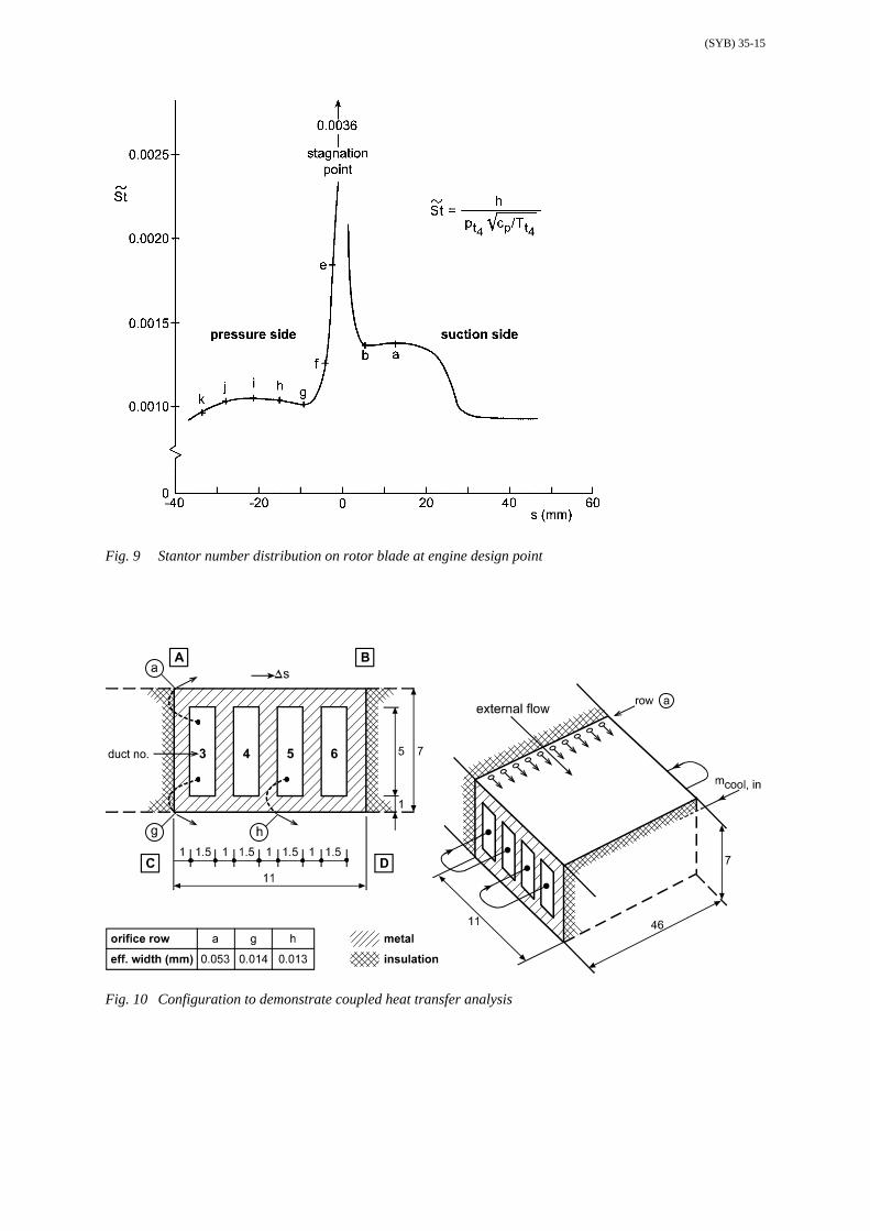
Figure 9 shows the Stanton number t~S distribution (defined at end of section 4) on the mid-span radius for thereference condition as a function of the distance s from the stagnation point measured along the blade surface.This stagnation point is assumed to be between orifice rows ‘c’ and ‘d’. The three non-dimensional engineoperation parameters at this condition are realised for pt4 = 2 MPa, Tt4 = 1200 K, N2 = 12500 rpm and p45 = 0.5MPa.

For the situation without film cooling the resulting heat transfer coefficients hext are obtained through

multiplication of t~S by pt4√(cp /Tt4) with p and T in Pa and K respectively. For the situation with film cooling alower value for the total temperature must be used than the turbine entry value Tt4 and hext will be accordinglyhigher. In fact a correction is made for the higher ρu value at the rotor blade. The procedure will be illustratedbelow for the engine design point.

(SYB) 35-7

At the engine design point pt4 = 2.137 MPa and Tt4 = 1675 K. Cooling air is entering the turbine inlet guidevanes at 821 K. During its passage through the IGV’s the air is heated up by the heat flowing from the externalblade surface to the cooling ducts. This heat is returning into the external flow by the film cooling air. It followsfrom the resulting heat balance that the total temperature behind the IGV’s must be calculated as a result ofmixing 45.3 kg combustion gas at 1675 K with 4.79 kg cooling air of 821 K. The result is a total temperature of1596 K in the stator frame of reference at the interface between the IGV’s and the rotor. It is assumed that thestagnation pressure remains unchanged and equal to 21.37 bar.

The result is that Tt4 = 1596 K and pt4 = 2.137 MPa must be used to calculate h from t~S as presented in figure

10 for the engine design point. For t~S = 0.001 a heat transfer coefficient hext = 1.88 kW/m2/K results.

CFD calculations predict a (rotor) relative Mach number 0.270 at the mid-span radius at the entry of the rotorcomputational domain. This results in Tt = 1509 K and pt = 16.75 bar in the rotor frame of reference at the mid-span radius r = 0.285 m. This temperature can be used as Tgas for the calculation of the film temperature forgiven ηfilm , see section 2.

9. Internal heat transfer and pressure losses

The cooling air flow will be heated on its way through the cooling duct and at the same time its total pressurewill reduce as a result of wall friction. Data from Ref.7 were used to estimate of the effect of the turbulators. It isassumed that for the present turbulator configuration the Stanton number St is increased by a factor 2 andSt/(cf)

1/3 by a factor 1.2 compared to the value of a turbulent fully developed pipe flow. So, cf increases by afactor 4.6.

Take for example a serpentine cooling duct with a flow Mach number 0.18 with ρu ≈ 700 (kg/s)/m2. Its crosssection is of 1.5 × 5 mm leading to a hydraulic diameter of 2.3 mm. Its length is 46 mm. The cooling air massflow is 5.2 g/s at T = 1000 K, p = 18 bar and the Reynolds number Red,hyd is 39 000. This leads to a heat transfercoefficient of 6 kW/m2/K. For a temperature difference of 100 K between the cooling air and the duct wall thecooling air temperature will increase 56 K in one duct length. Along this duct the total pressure decreases by 4.4percent. These calculations can be improved in further iteration steps.

Orifice flow pressure losses are estimated at 1.3 percent per diameter length with a turbulent pipe flow model.The orifice heat transfer coefficient is estimated at 10 kW/m2/K. Taking ρu ≈ 2200 (kg/s)/m2 (sonic flow,discharge coefficient 0.8), an orifice diameter of 0.25 mm and an orifice length of 10 diameters, the cooling airtemperature is increased by 16 K across the orifice for 100 K temperature difference between the orifice walland the cooling air.

10. Coupled heat transfer calculations

10.1 Simple geometry modelFor prediction of the temperature distribution in the rotor blade material an iterative calculation procedure isrequired as described in section 2. Before performing these calculations on the actual rotor blade a computationwas made on the simple configuration shown in figure 10, in fact representing the serpentine cooling ductsrunning along the full blade length of 46 mm.

The side A-B represents part of the blade suction side and C-D part of the pressure side. Cooling air enters duct6 at a total pressure and temperature of 19.6 bar and 875 K (602 °C). In duct 5 part of the cooling air is ejectedthrough a row of orifices ‘h’ with a total geometric area of 0.75 mm2. In duct 3 the remaining cooling air isejected through orifices ‘a’ with a total geometric area of 3.0 mm2 and ‘g’ with a total geometric area of 0.8mm2. External total pressure and temperature are 16.75 bar and 1509 K. At the suction side A-B the localexternal flow Mach number is 0.6 and at the pressure side C-D this is 0.25. The external heat transfer coefficient

is 2.6 kW/m2/K at the suction side A-B and 2 kW/m2/K at the pressure side C-D. This corresponds to t~S =0.0138 and 0.0106 (see figure 9). The internal heat transfer coefficient in the serpentine ducts is 7 kW/m2/K.This is slightly higher than the value mentioned in section 9. Orifice heat transfer is neglected. Somecompensation is found by taking the injection temperature for the full row equal to the local total temperature inthe end of the cooling duct (i.e. at the last orifice). The heat conductivity of the blade material is λ = 20 W/m/K.

(SYB) 35-8

10.2 Estimate of cooling air mass flowsThe first step is to estimate the cooling air mass flow in the serpentine ducts. This is done by an iterativeprocedure starting with an assumed total pressure halfway duct 3 that must be higher than the external pressureof 16.09 bar at ‘g’. Using a pressure ratio dependent discharge coefficient obtained from Ref.5, the orifice massflow is determined assuming a total temperature of 1050 K in duct 3. The mass flow in duct 4 is known and thepressure drop due to friction (4.6 times the value in a smooth pipe) can be calculated. Assumed average coolingair temperatures in ducts 4, 5 and 6 are 1000, 950 and 900 K. After including the mass flow from orifice row ‘h’the pressure at the entry of duct 6 is calculated and compared to the target value of 19.6 bar. After iteration thefollowing results are found (using air with a specific heat ratio γ = 4/3 internally and 1.3 externally). Machnumbers and velocities u are in the ducts (4 and 6) or in the jets from the cooling orifices (a, g and h).

pt pext CD mass flow Mach ubar bar g./s m/s

orifice row A 17.20 13.34 0.70 4.05 0.636 390orifice row G 17.20 16.09 0.69 0.60 0.318 200duct (mid) 4 17.84 - - 4.65 0.160 98.9orifice row H 18.48 16.09 0.72 0.90 0.460 273duct entry 6 19.65 - - 5.55 0.172 100.8

These mass flows are used in the calculation of the blade temperature distribution and the actual cooling airtemperature in the serpentine ducts using the FEM model for the heat conduction inside the blade material.

10.3 Orifice versus slot coolingTwo cases are considered. One is the case with orifice film cooling with an assumed efficiency of 0.15. Theother case is with slot cooling, starting with an efficiency of 0.8 at the slots and decreasing linearly downstreamat a rate of 0.05 per mm. At rows ‘a’ and ‘g’ the upstream adiabatic wall temperature is taken equal to 1500 K =1227 °C and at row ‘h’ this is taken equal to the local film temperature behind row ‘g’.

The FEM calculations are started with a uniform temperature of the blade material. After 15 minutescomputation time on a work station and using 7 iteration steps, an accuracy of better than 1 degree C isobtained.

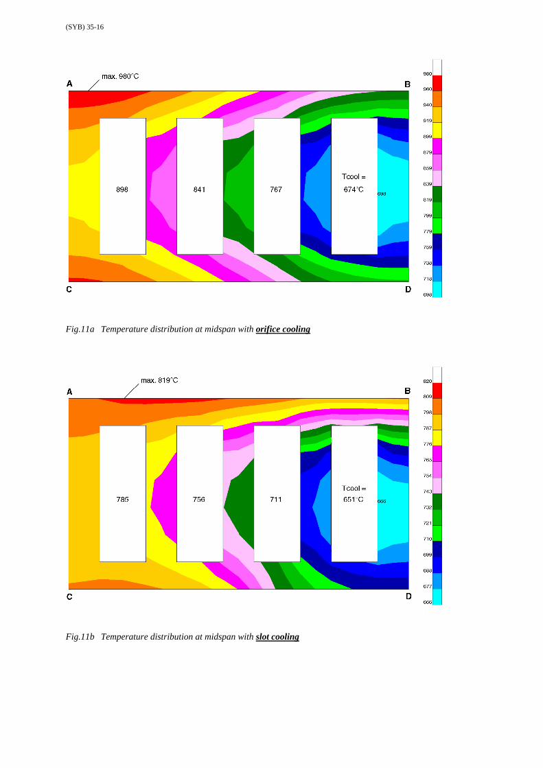
In figure 11 the resulting blade material temperatures are presented as well as the cooling flow temperatures atmid-span. Temperatures are given in degrees Celsius since this unit is very often used when materials propertiesare discussed.

It is noted that the air temperatures in the cooling ducts are higher than assumed when estimating the mass flowsto evaluate the pressure loss in section 10.2. At orifice rows ‘a’ and ‘g’ the total temperature is 898 + 273 =1171 K rather than 1050 K. This results in a 5.3 percent lower mass flow. This would require a second iterationcycle, not performed here.

The injection temperature is taken constant along the blade span and equal to the cooling air temperature at theend of the serpentine duct that feeds the orifices. The result is that the maximum temperature of the “bladesegment” is found on the upper (suction) side near the end of the duct ‘3’. This temperature is slightly higherthan the value at mid span.

The maximum material temperature is 989 °C in the case of orifice cooling with a local film cooling efficiencyof 0.15. The mid-span value is 980 °C, see figure 11. The injection temperature for row ‘a’ is 923 °C and theresulting film temperature is 1181 °C.

In the case of slot cooling the maximum material temperature is 825 °C (a reduction of 164 °C) and 819 °C isfound at mid span. Without adaptation, a CFD model representing orifice cooling by a slot cooling model willlead to unrealistic results for the present application.

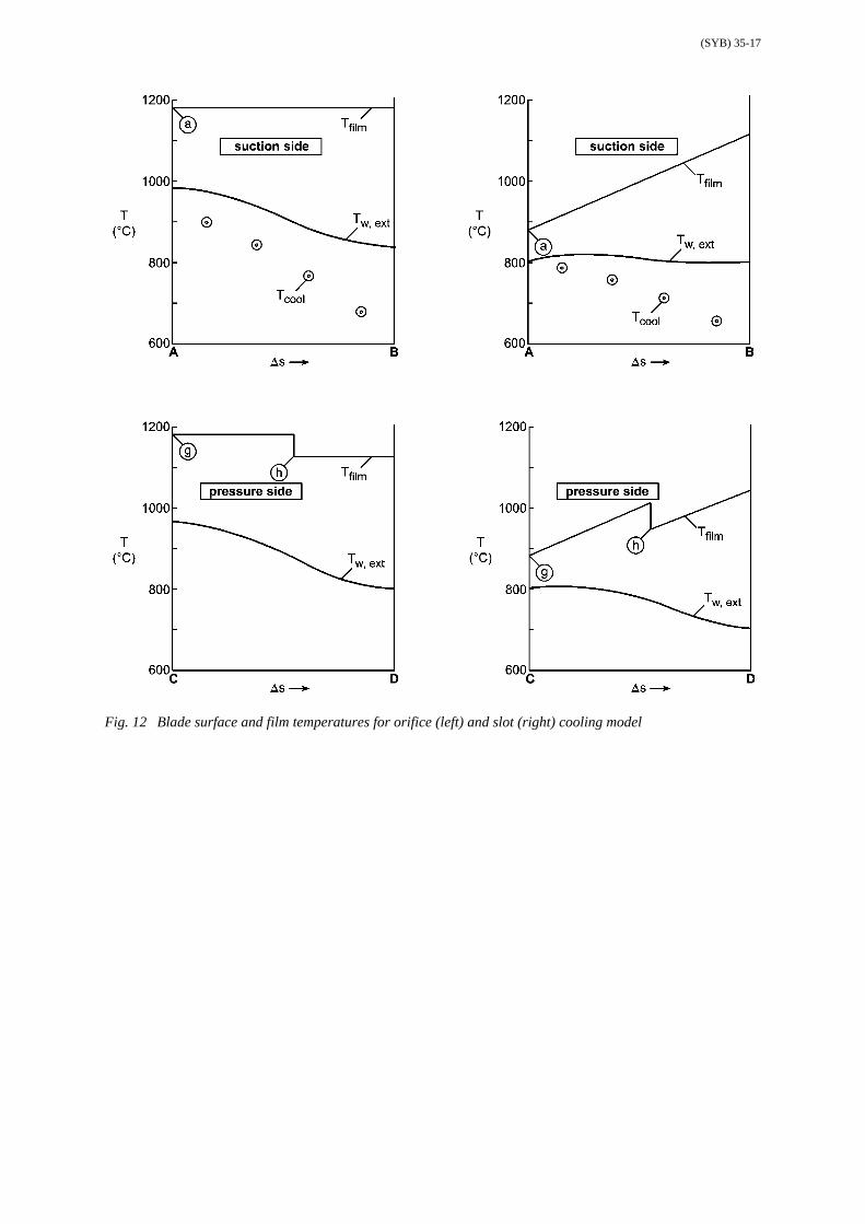
Figure 12 shows the blade surface temperature distribution at mid-span according to fig.11 and thecorresponding film temperature resulting from the assumed film cooling efficiencies. For both cooling methodsthe highest heat transfer is found at the downstream edge (points B and D). At point B a heat transfer of 345 ×2.7 = 932 kW/m2 is found for the orifice cooling model and 318 × 2.7 = 859 kW/m2 for the slot cooling model.

Temperature gradients in the blade material are of the order of 50 °C/mm and are maximum in the top wall ofthe first cooling duct where the temperature in the cooling ducts is low. If a flat plate is heated on one side such

(SYB) 35-9

that a temperature difference of 50 °C exists between the two sides and this plate is forced to remain planar,thermal stresses will develop. For a thermal expansion coefficient ε = 13 E-6 per deg C and a Youngs modulusE = 2.0 E+5 N/mm2 a stress level is calculated of 65 / 0.7 = 93 N/mm2. These material values are for a nickelalloy at room temperature. At higher temperatures E may be lower but this example illustrates that significantthermal stresses will exist that have to be analysed further and be related to creep and thermal fatigue, alsotaking into account the aerodynamic and centrifugal loads that occur.

10.4 Sensitivity to input dataThe simple geometry model of figure 10 was used further to estimate the effect of variation of input data on themaximum blade temperature, using the orifice film cooling model and its results (Fig 11a and 12 left) asbaseline. The following temperatures were found, changing one parameter as indicated while the others remainunchanged:

Temp in°C Max walltemp

Max wall tempat mid span

Injection tempof row “a”

Film temp behindrow “a”

Baseline 989 980 923 11811.25 hint 975 965 901 11781.25 hext 1027 1018 954 11861.25 mcool 962 953 877 11750.8 mcool 1025 1017 968 1188ηfilm = 0.15 → 0.25 961 952 895 1144Tcool,in = 602 → 677 1019 1011 957 1187Tgas = 1227 → 1377 1083 1072 996 1320

The last row corresponds to an increase of the gas temperature by 10 percent from 1500 to 1650K (in the rotorframe of reference). This would correspond to a turbine entry temperature that is 10 percent higher than the(area) average value at the engine design point according to GSP. The resulting blade temperature in this casemay indicate the value that would result from a temperature distortion in the radial direction with a peaktemperature at mid span 10 percent above the area average value. The resulting value for the profile factordefined as (Tt4,max,rad − Tt4,avg)/(Tt4,avg − Tt3) is 168 / (1675 − 821 ) = 0.197 (see also Ref. 8).

With this simulated temperature distortion a maximum materials temperature of 1083 °C results. This is close tothe maximum short-time use temperature of the single crystal nickel alloys that are used in the F100-PW-220engine.

The maximum (area average) turbine entry temperature that may occur during a flight mission is somewhathigher than the value of 1675 K (1402 °C) at the design point (sea level military thrust). On the other hand thefilm temperature at rows ‘a” and “g” will be lowered by the upstream orifice rows. This is not taken into accountwhen calculating the film temperature behind these rows on the cooling block model of figure 10.

It is concluded that the present analysis provides a suitable method to calculate blade temperature historiessufficiently accurate to estimate engine blade life on a relative basis using the engine operational conditions ascollected by the flight data recording system.

11. Conclusions

A method has been formulated to predict the temperature distribution in film cooled turbine blades. Input dataare: the engine operational conditions and the geometry of the vanes and blades including the size and locationof the film cooling orifices.

The input data are used as follows:1. The Gas Turbine Simulation Program GSP translates the operational conditions in turbine entry and exit

temperatures, pressures and mass flows including cooling air.2. The distribution of the cooling air between the various blade rows is estimated from the orifice area and

assumed cooling air pressures and temperatures inside the blades.3. FINE/Turbo calculates the pressure and heat transfer coefficient distribution on the rotor blade without

film cooling as well as the pressure distribution with film cooling using turbine entry and exit conditionsfrom GSP. These heat transfer coefficients are also used for the situation with film cooling.

(SYB) 35-10

4. The internal heat transfer and pressure losses are estimated taking the values in fully developed turbulentpipe flows multiplied by factors to account for the presence of turbulators. These factors are typically 2and 5 respectively.

5. The film cooling efficiency is a free variable and is typically 0.2 to 0.1 for orifice film cooling.

The following lessons have been learned:1. CFD methods require very fine computational grids to realistically capture the flow and heat transfer near

the film cooling injection orifices. At present this leads to computation times that are out-of-balance withan analysis that relates engine operational conditions during a flight mission to blade temperatures.

2. Modelling cooling orifices by means of a slot width of 1 to 5 percent of the blade chord can be usedefficiently to calculate the effect of added mass by film cooling on the blade pressure distributions.

3. The value of film cooling efficiency is one of the most uncertain factors in the prediction of the bladetemperatures when real blades with cooling orifices of optimised orientation are considered. Themaximum materials temperature predicted with an orifice cooling efficiency of 0.15 is close to themaximum short-time use temperature of single crystal nickel alloys.

5. The present analysis provides a suitable method to calculate blade temperature histories sufficientlyaccurate to estimate engine blade life on a relative basis using the engine operational conditions ascollected by the flight data recording system.

12. References

1. Colladay, R.S.; Turbine Cooling, Chapter 11 in: Turbine Design and Application, NASA SP-290 (1994).2. Sellers, J.P.; Gaseous Film Cooling with Multiple Injection Stations, AIAA J. Sept. 1963, pp. 2154-2156.3. Kadotani, K, and Goldstein, R.J.; Effect of Mainstream Variables on Jets Issuing from a Row of Inclined

Round Holes J. Eng. for Power, April 1979, Vol. 101, pp 298-304.4. Visser, W.P.J.; GSP, A Generic Object-Oriented Gas Turbine Simulation Environment, ASME-2000-GT-

0002, NLR-TP-2000-267.5. Gritsch, M., Schultz, A. and Wittig, S.; Method for Correlating Discharge Coefficients of Film Cooling

Holes, AIAA J Vol.36, No.6, June 1998, pp 976-980).6. Numeca International, FINE/Turbo User Manual (version 4.1), Numeca International, Brussels, April

2000.7. Harasgama, S.P.; Aerothermal Aspects in Gas Turbine Flows: Turbine Blade Internal Cooling, VKI

Lecture Series 1995-05.8. Van Erp, C.A. and Richman, M.H.; Technical Challenges Associated with the Development of Advanced

Combustion Systems, Paper 3 in RTO-MP-14, 1999.

(SYB) 35-11

Fig. 1 Multi-disciplinary framework for life prediction model

Fig. 2 HP turbine exit temperature variation of F-100-PW-220 turbofan engine recorded during anF-16 mission

(SYB) 35-12

Fig. 3 Data flow logic in film cooling heat transfer calculations

Fig. 4 F-100-PW-220 HP turbine blades at mid-span with grid used for CFD computations

(SYB) 35-13

Fig. 5 F-100-PW-220 high-pressure turbine inlet guide vanes and first stage rotor blade

Fig. 6 First stage rotor blade with cooling ducts and film cooling orifices

(SYB) 35-14

Fig. 7 Relative Mach numbers in HP-turbine at engine reference conditions

Fig. 8 Mach number on rotor blade outside the boundary layer as derived fromsurface pressure calculations

(SYB) 35-15

Fig. 9 Stantor number distribution on rotor blade at engine design point

Fig. 10 Configuration to demonstrate coupled heat transfer analysis

(SYB) 35-16

Fig.11a Temperature distribution at midspan with orifice cooling

Fig.11b Temperature distribution at midspan with slot cooling

(SYB) 35-17

Fig. 12 Blade surface and film temperatures for orifice (left) and slot (right) cooling model

This page has been deliberately left blank

Page intentionnellement blanche