Copyright c© 2006 Tech Science Press CMES, vol.12, no.2, pp.109-119, 2006

Analysis of Circular Torsion Bar with Circular Holes Using Null-field Approach

Jeng-Tzong Chen 1, Wen-Cheng Shen 2, Po-Yuan Chen 2

Abstract: In this paper, we derive the null-field inte-gral equation for a circular bar weakened by circular cav-ities with arbitrary radii and positions under torque. Tofully capture the circular geometries, separate forms offundamental solution in the polar coordinate and Fourierseries for boundary densities are adopted. The solutionis formulated in a manner of a semi-analytical form sinceerror purely attributes to the truncation of Fourier series.Torsion problems are revisited to demonstrate the validityof our method. Torsional rigidities for different numberof holes are also discussed.

keyword: Torsion, Null-field integral equation,Fourier series, Circular hole, Torsional rigidity.

1 Introduction

Boundary value problems always involve several holesor more than one important reference point. It is con-venient to be able to expand the solutions in alternativeways, each way referring to different specific coordinateset describing the same solution. According to the idea,we develop a systematic approach including the adaptiveobserver system and degenerate kernel for fundamentalsolution in the polar coordinate and employ Fourier se-ries to approximate the boundary data.

In the past, multiply connected problems have been car-ried out either by conformal mapping or by special tech-niques. Ling [Ling C. B. (1947)] solved the torsionproblem of a circular tube with several holes. Muskhel-ishvili [Muskhelishvili N. I. (1953)] solved the problemof a circular bar reinforced by an eccentric circular in-clusion. Chen and Weng [Chen T.; Weng I. S. (2001)]have introduced conformal mapping with a Laurent se-ries expansion to analyze the Saint-Venant torsion prob-lem. They concerned with a eccentric bar of different ma-

1 Distinguished Professor, Department of Harbor and River En-gineering, National Taiwan Ocean University, Keeling, Taiwan.Email: jtchen@mail.ntou.edu.tw

2 Graduate student, Department of Harbor and River Engineering,National Taiwan Ocean University, Keeling, Taiwan.

terials with an imperfect interface under torque. Basedon the CVBEM (complex variable boundary elementmethod), Shams-Ahmadi and Chou [Shams-Ahmadi M.;Chou S. I. (1997)] have investigated the torsion prob-lem of composite shafts with any number of inclusionsof different materials. Recently, Ang and Kang [AngW. T.; Kang I. (2000)] developed a general formulationfor solving the second-order elliptic partial differentialequation for a multiply-connected region in a differentversion of CVBEM. To avoid mesh generation for finiteelement or boundary element, meshless formulation isa promising direction [Jin B. (2004), Sladek V.; SladekJ.; Tanaka M. (2005), Wordelman C. J.; Aluru N. R.;Ravaioli U. (2000)]. The present formulation can beseen as one kind of meshless methods, since it belongsto boundary collocation methods. Because the confor-mal mapping is limited to the doubly connected region,an increasing number of researchers have paid more at-tentions on special solutions. However, the extensionto multiple circular holes may encounter difficulty. Itis not trivial to develop a systematic method for solv-ing the torsion problems with several holes. Crouch andMogilevskaya [Crouch S. L.; Mogilevskaya S. G. (2003)]utilized Somigliana’s formula and Fourier series for elas-ticity problems with circular boundaries. Mogilevskayaand Crouch [Mogilevskaya S. G.; Crouch S. L. (2001)]have solved the problem of an infinite plane containingarbitrary number of circular inclusions based on the com-plex singular integral equation. In their analysis pro-cedure, the unknown tractions are approximated by us-ing the complex Fourier series. However, for calculat-ing an integral over a circular boundary, they didn’t ex-press the fundamental solution using the local polar co-ordinate. By moving the null-field point to the bound-ary, the boundary integral can be easily determined us-ing series sums in our formulation due to the introduc-tion of degenerate kernels. Mogilevskaya and Crouch[Mogilevskaya S. G.; Crouch S. L. (2001)] have used theGalerkin method to approach boundary density insteadof collocation approach. Our approach can be extendedto the Galerkin formulation only for the circular and an-

110 Copyright c© 2006 Tech Science Press CMES, vol.12, no.2, pp.109-119, 2006

nular cases. However, it may encounter difficulty for theeccentric case. Two requirements are needed: degeneratekernel expansion must be available and distinction of in-terior and exterior expression must be separated. There-fore, the collocation angle of φ is not in the range 0 to2π in our adaptive observer system. This is the reasonwhy we can not formulate in terms of Galerkin formula-tion using orthogonal properties twice. Free of worryinghow to choose the collocation points, uniform collocationalong the circular boundary yields a well-posed matrix.On the other hand, Bird and Steele [Bird M. D.; SteeleC. R. (1991)] have also used separated solution proce-dure for bending of circular plates with circular holes ina similar way of the Trefftz method and addition theorem.

In this paper, the null-field integral equation is utilizedto solve the Saint-Venant torsion problem of a circularshaft weakened by circular holes. The mathematical for-mulation is derived by using degenerate kernels for fun-damental solution and Fourier series for boundary den-sity in the null-field integral equation. Then, it reducesto a linear algebraic equation. After determining the un-known Fourier coefficients, series solutions for the warp-ing function and torsional rigidity are obtained. Numeri-cal examples are given to show the validity and efficiencyof our formulation.

2 Formulation of the problem

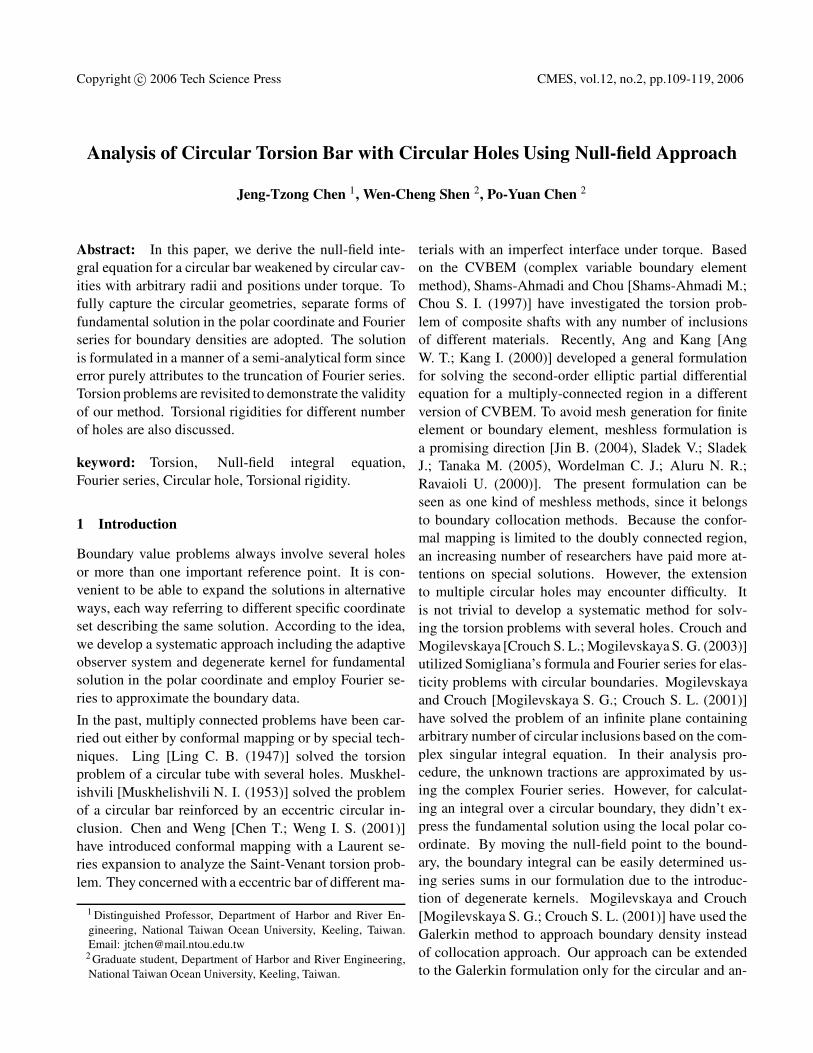
What is given in Figure 1 is a circular bar weakened byN circular holes placed on a concentric ring of radius b.

Figure 1 : Cross section of bar weakened byN (N = 3) equal circular holes

The radii of the outer circle and the inner holes are Rand a, respectively. The circular bar twisted by couplesapplied at the ends is taken into consideration. Follow-ing the theory of Saint-Venant torsion [Timoshenko S. P.;Goodier J. N. (1970)], we assume the displacement fieldto be

u = −αyz, v = αxz, w = αϕ(x,y), (1)

where α is the angle of twist per unit length along the zdirection and ϕ is the warping function. According to thedisplacement field in Eq. (1), the strain components are

εx = εy = εz = γxy = 0, (2)

γxz =∂w∂x

+∂u∂z

= α(∂ϕ∂x

−y), (3a)

γyz =∂w∂y

+∂v∂z

= α(∂ϕ∂y

+x), (3b)

and their corresponding components of stress are

σx = σy = σz = σxy = 0, (4)

σxz = µα(∂ϕ∂x

−y), σyz = µα(∂ϕ∂y

+x), (5)

where µ is the shear modulus. There is no distortion inthe planes of cross sections since εx = εy = εz = γxy = 0.We have the state of pure shear at each point defined bythe stress components σxz and σyz. The warping functionϕ must satisfy the equilibrium equation

∂2ϕ∂x2 +

∂2ϕ∂y2 = 0 in D , (6)

where the body force is neglected and D is the domain.Since there are no external forces on the cylindrical sur-face, we have tx = ty = tz = 0. By substituting the normalvector, the only zero tz becomes

tz = σxznx +σyzny = 0 on B. (7)

By substituting (5) into (7) and rearranging, the boundarycondition is

∂ϕ∂x

nx +∂ϕ∂y

ny = ynx −xny = ∇ϕ ·n =∂ϕ∂n

on B, (8)

Analysis of Circular Torsion Bar 111

where B is the boundary. In Figure 1, we introduce theexpressions for the position vector (xk,yk) of the bound-ary point on the kth circular hole

xk = acosθk +bcos(2πkN

), k = 1, 2, · · · , N,

0 < θk < 2π, (9)

yk = asinθk +bsin(2πkN

), k = 1, 2, · · · , N,

0 < θk < 2π, (10)

and the unit outward normal vector n = (nx,ny) =(−cosθ,−sinθ) for the inner circular boundaries, wehave

∂ϕ∂n

= bcos(2πkN

) sinθk −bsin(2πkN

)cosθk on Bk,

(11)

where Bk (k = 1, 2, · · · , N) is the kth boundary of theinner hole, θk is the polar angle with respect to the originof the kth hole. For the outer boundary, the traction-freecondition is specified. Thus, the problem of torsion isreduced to find the warping function ϕ which satisfiesLaplace equation of Eq. (6) and the Neumann boundaryconditions of Eq. (11) for the inner boundary and zerotraction on the outer boundary.

3 Method of solution

3.1 The dual boundary integral equations and null-field integral equations

We apply the Fourier series expansions to approximatethe potential u and its normal derivative on the boundary

u(sk) = ak0 +

∞

∑n=1

(akn cosnθk +bk

n sinnθk),

sk ∈ Bk, k = 1, 2, · · · , N, (12)

t(sk) = pk0 +

∞

∑n=1

(pkn cosnθk +qk

n sinnθk),

sk ∈ Bk, k = 1, 2, · · · , N, (13)

where t(sk) = ∂u(sk)/∂ns, akn, bk

n, pkn and qk

n (n =0, 1, 2, · · ·) are the Fourier coefficients and θk is the po-lar angle. The integral equation for the domain point can

be derived from the third Green’s identity [Chen, J. T.;Hong, H. -K. (1999)], we have

2πu(x) =Z

BT (s,x)u(s)dB(s)−

ZB

U(s,x)t(s)dB(s),

x ∈ D, (14)

2π∂u(x)∂nx

=Z

BM(s,x)u(s)dB(s)−

ZB

L(s,x)t(s)dB(s),

x ∈ D, (15)

where s and x are the source and field points, respectively,D is the domain of interest, ns and nx denote the outwardnormal vectors at the source point s and field point x,respectively, and the kernel function U(s,x) = lnr, (r ≡|x− s|), is the fundamental solution which satisfies

∇2U(s,x) = 2πδ(x− s), (16)

in which δ(x− s) denotes the Dirac-delta function. Theother kernel functions, T (s,x), L(s,x) and M(s,x), aredefined by

T (s,x)≡ ∂U(s,x)∂ns

, L(s,x)≡ ∂U(s,x)∂nx

,

M(s,x)≡ ∂2U(s,x)∂ns∂nx

, (17)

By collocating x outside the domain (x ∈ Dc), we obtainthe dual null-field integral equations as shown below

0 =Z

BT (s,x)u(s)dB(s)−

ZB

U(s,x)t(s)dB(s),

x ∈ Dc, (18)

0 =Z

BM(s,x)u(s)dB(s)−

ZB

L(s,x)t(s)dB(s),

x ∈ Dc, (19)

where Dc is the complementary domain. Based on theseparable property, the kernel function U(s,x) can be ex-panded into degenerate form by separating the sourcepoints and field points in the polar coordinate [Chen J.T.; Chiu Y. P. (2002)]:

U(s,x) =

⎧⎪⎪⎪⎪⎪⎨⎪⎪⎪⎪⎪⎩

Ui(R,θ;ρ,φ)= lnR

− ∞∑

m=1

1m( ρ

R)m cosm(θ−φ), R ≥ ρ

Ue(R,θ;ρ,φ) = lnρ

−∞∑

m=1

1m(R

ρ )m cosm(θ−φ), ρ > R

(20)

112 Copyright c© 2006 Tech Science Press CMES, vol.12, no.2, pp.109-119, 2006

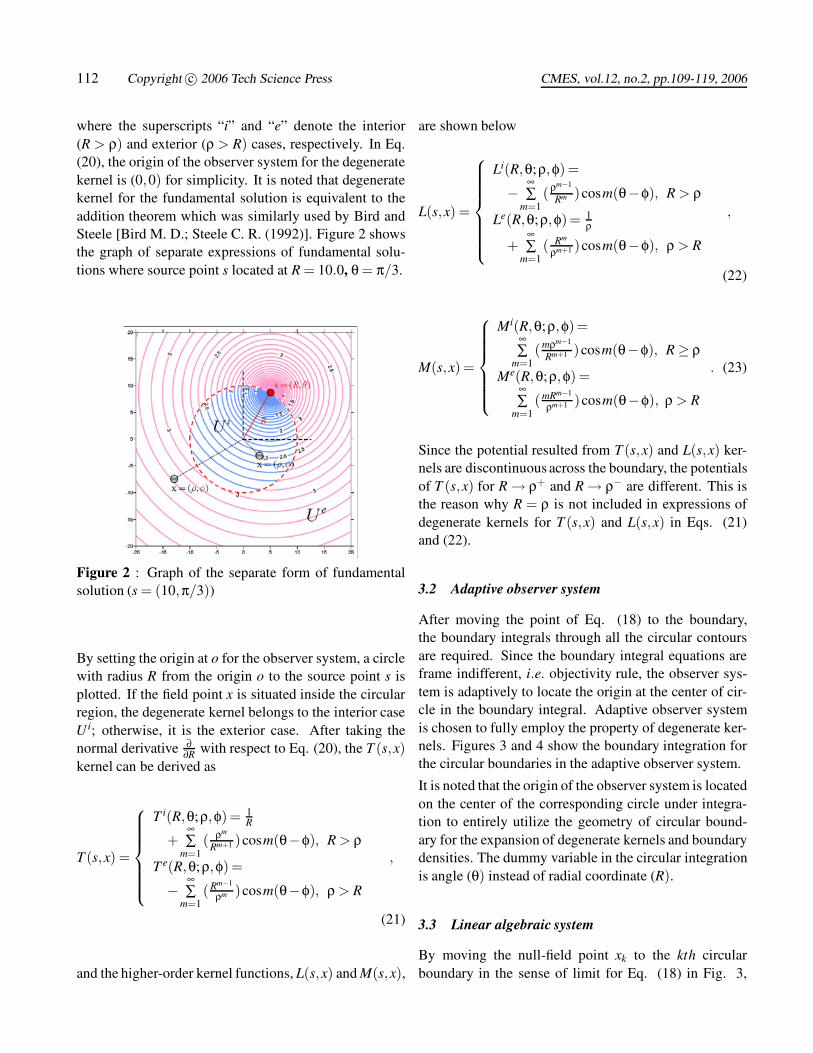
where the superscripts “i” and “e” denote the interior(R > ρ) and exterior (ρ > R) cases, respectively. In Eq.(20), the origin of the observer system for the degeneratekernel is (0,0) for simplicity. It is noted that degeneratekernel for the fundamental solution is equivalent to theaddition theorem which was similarly used by Bird andSteele [Bird M. D.; Steele C. R. (1992)]. Figure 2 showsthe graph of separate expressions of fundamental solu-tions where source point s located at R = 10.0, θ = π/3.

Figure 2 : Graph of the separate form of fundamentalsolution (s = (10,π/3))

By setting the origin at o for the observer system, a circlewith radius R from the origin o to the source point s isplotted. If the field point x is situated inside the circularregion, the degenerate kernel belongs to the interior caseUi; otherwise, it is the exterior case. After taking thenormal derivative ∂

∂R with respect to Eq. (20), the T (s,x)kernel can be derived as

T (s,x) =

⎧⎪⎪⎪⎪⎪⎨⎪⎪⎪⎪⎪⎩

T i(R,θ;ρ,φ)= 1R

+∞∑

m=1( ρm

Rm+1 )cosm(θ−φ), R > ρ

T e(R,θ;ρ,φ) =

−∞∑

m=1(Rm−1

ρm )cosm(θ−φ), ρ > R

,

(21)

and the higher-order kernel functions, L(s,x) and M(s,x),

are shown below

L(s,x) =

⎧⎪⎪⎪⎪⎪⎪⎨⎪⎪⎪⎪⎪⎪⎩

Li(R,θ;ρ,φ) =

−∞∑

m=1(ρm−1

Rm )cosm(θ−φ), R > ρ

Le(R,θ;ρ,φ)= 1ρ

+∞∑

m=1( Rm

ρm+1 )cosm(θ−φ), ρ > R

,

(22)

M(s,x) =

⎧⎪⎪⎪⎪⎪⎨⎪⎪⎪⎪⎪⎩

Mi(R,θ;ρ,φ)=∞∑

m=1(mρm−1

Rm+1 )cosm(θ−φ), R ≥ ρ

Me(R,θ;ρ,φ) =∞∑

m=1(mRm−1

ρm+1 )cosm(θ−φ), ρ > R

. (23)

Since the potential resulted from T (s,x) and L(s,x) ker-nels are discontinuous across the boundary, the potentialsof T (s,x) for R → ρ+ and R → ρ− are different. This isthe reason why R = ρ is not included in expressions ofdegenerate kernels for T (s,x) and L(s,x) in Eqs. (21)and (22).

3.2 Adaptive observer system

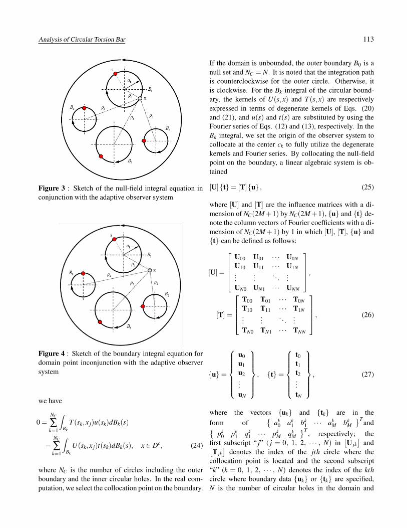
After moving the point of Eq. (18) to the boundary,the boundary integrals through all the circular contoursare required. Since the boundary integral equations areframe indifferent, i.e. objectivity rule, the observer sys-tem is adaptively to locate the origin at the center of cir-cle in the boundary integral. Adaptive observer systemis chosen to fully employ the property of degenerate ker-nels. Figures 3 and 4 show the boundary integration forthe circular boundaries in the adaptive observer system.

It is noted that the origin of the observer system is locatedon the center of the corresponding circle under integra-tion to entirely utilize the geometry of circular bound-ary for the expansion of degenerate kernels and boundarydensities. The dummy variable in the circular integrationis angle (θ) instead of radial coordinate (R).

3.3 Linear algebraic system

By moving the null-field point xk to the kth circularboundary in the sense of limit for Eq. (18) in Fig. 3,

Analysis of Circular Torsion Bar 113

Figure 3 : Sketch of the null-field integral equation inconjunction with the adaptive observer system

Figure 4 : Sketch of the boundary integral equation fordomain point inconjunction with the adaptive observersystem

we have

0 =NC

∑k=1

ZBk

T (sk,x j)u(sk)dBk(s)

−NC

∑k=1

ZBk

U(sk,x j)t(sk)dBk(s), x ∈ Dc, (24)

where NC is the number of circles including the outerboundary and the inner circular holes. In the real com-putation, we select the collocation point on the boundary.

If the domain is unbounded, the outer boundary B0 is anull set and NC = N. It is noted that the integration pathis counterclockwise for the outer circle. Otherwise, itis clockwise. For the Bk integral of the circular bound-ary, the kernels of U(s,x) and T (s,x) are respectivelyexpressed in terms of degenerate kernels of Eqs. (20)and (21), and u(s) and t(s) are substituted by using theFourier series of Eqs. (12) and (13), respectively. In theBk integral, we set the origin of the observer system tocollocate at the center ck to fully utilize the degeneratekernels and Fourier series. By collocating the null-fieldpoint on the boundary, a linear algebraic system is ob-tained

[U]{t}= [T]{u} , (25)

where [U] and [T] are the influence matrices with a di-mension of NC(2M +1) by NC(2M +1), {u} and {t} de-note the column vectors of Fourier coefficients with a di-mension of NC(2M + 1) by 1 in which [U], [T], {u} and{t} can be defined as follows:

[U] =

⎡⎢⎢⎢⎣

U00 U01 · · · U0N

U10 U11 · · · U1N...

.... . .

...UN0 UN1 · · · UNN

⎤⎥⎥⎥⎦ ,

[T] =

⎡⎢⎢⎢⎣

T00 T01 · · · T0N

T10 T11 · · · T1N...

.... . .

...TN0 TN1 · · · TNN

⎤⎥⎥⎥⎦ , (26)

{u} =

⎧⎪⎪⎪⎪⎪⎨⎪⎪⎪⎪⎪⎩

u0

u1

u2...uN

⎫⎪⎪⎪⎪⎪⎬⎪⎪⎪⎪⎪⎭

, {t} =

⎧⎪⎪⎪⎪⎪⎨⎪⎪⎪⎪⎪⎩

t0

t1

t2...tN

⎫⎪⎪⎪⎪⎪⎬⎪⎪⎪⎪⎪⎭

, (27)

where the vectors {uk} and {tk} are in the

form of{

ak0 ak

1 bk1 · · · ak

M bkM

}Tand{

pk0 pk

1 qk1 · · · pk

M qkM

}T, respectively; the

first subscript “ j” ( j = 0, 1, 2, · · · , N) in[U jk

]and[

T jk]

denotes the index of the jth circle where thecollocation point is located and the second subscript“k” (k = 0, 1, 2, · · · , N) denotes the index of the kthcircle where boundary data {uk} or {tk} are specified,N is the number of circular holes in the domain and

114 Copyright c© 2006 Tech Science Press CMES, vol.12, no.2, pp.109-119, 2006

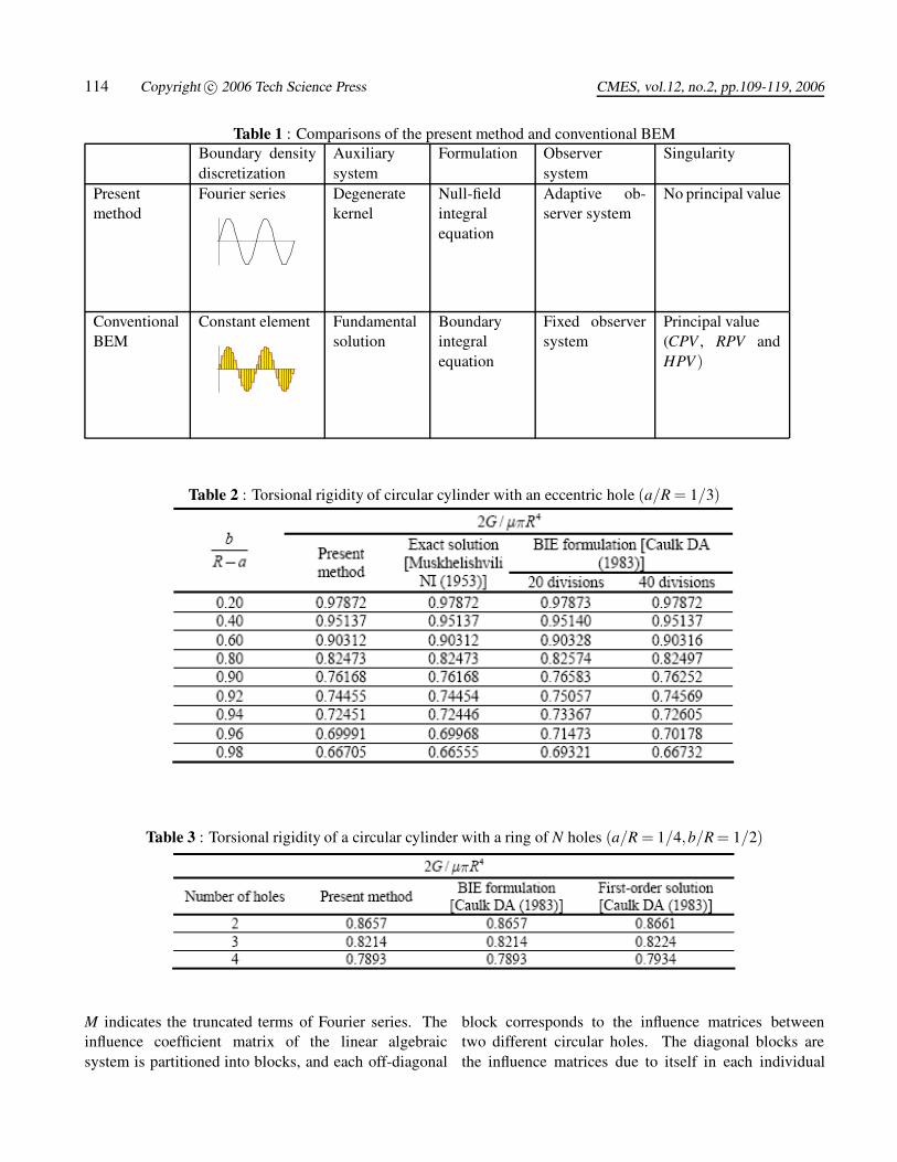
Table 1 : Comparisons of the present method and conventional BEMBoundary densitydiscretization

Auxiliarysystem

Formulation Observersystem

Singularity

Presentmethod

Fourier series Degeneratekernel

Null-fieldintegralequation

Adaptive ob-server system

No principal value

ConventionalBEM

Constant element Fundamentalsolution

Boundaryintegralequation

Fixed observersystem

Principal value(CPV , RPV andHPV)

Table 2 : Torsional rigidity of circular cylinder with an eccentric hole (a/R = 1/3)

Table 3 : Torsional rigidity of a circular cylinder with a ring of N holes (a/R = 1/4,b/R = 1/2)

M indicates the truncated terms of Fourier series. Theinfluence coefficient matrix of the linear algebraicsystem is partitioned into blocks, and each off-diagonal

block corresponds to the influence matrices betweentwo different circular holes. The diagonal blocks arethe influence matrices due to itself in each individual

Analysis of Circular Torsion Bar 115

hole. After uniformly collocating the point along the kthcircular boundary, the submatrix can be written as

[U jk

]=

⎡⎢⎢⎢⎢⎢⎢⎢⎢⎣

U0cjk (φ1) U1c

jk (φ1) U1sjk (φ1)

U0cjk (φ2) U1c

jk (φ2) U1sjk (φ2)

U0cjk (φ3) U1c

jk (φ3) U1sjk (φ3)

......

...U0c

jk (φ2M) U1cjk (φ2M) U1s

jk (φ2M)U0c

jk (φ2M+1) U1cjk (φ2M+1) U1s

jk (φ2M+1)

· · · UMcjk (φ1) UMs

jk (φ1)· · · UMc

jk (φ2) UMsjk (φ2)

· · · UMcjk (φ3) UMs

jk (φ3). . .

......

· · · UMcjk (φ2M) UMs

jk (φ2M)· · · UMc

jk (φ2M+1) UMsjk (φ2M+1)

⎤⎥⎥⎥⎥⎥⎥⎥⎥⎦

, (28)

[T jk

]=

⎡⎢⎢⎢⎢⎢⎢⎢⎢⎣

T 0cjk (φ1) T 1c

jk (φ1) T 1sjk (φ1)

T 0cjk (φ2) T 1c

jk (φ2) T 1sjk (φ2)

T 0cjk (φ3) T 1c

jk (φ3) T 1sjk (φ3)

......

...T 0c

jk (φ2M) T 1cjk (φ2M) T 1s

jk (φ2M)T 0c

jk (φ2M+1) T 1cjk (φ2M+1) T 1s

jk (φ2M+1)

· · · T Mcjk (φ1) T Ms

jk (φ1)· · · T Mc

jk (φ2) T Msjk (φ2)

· · · T Mcjk (φ3) T Ms

jk (φ3). . .

......

· · · T Mcjk (φ2M) T Ms

jk (φ2M)· · · T Mc

jk (φ2M+1) T Msjk (φ2M+1)

⎤⎥⎥⎥⎥⎥⎥⎥⎥⎦

. (29)

Although the matrices in Eqs. (28) and (29) are notsparse, they are diagonally dominant. It is found thatthe influence coefficient for the higher-order harmonicsis smaller. It is noted that the superscript “0s” in Eqs.(28) and (29) disappears since sinθ = 0. The element of[U jk

]and

[T jk

]are defined respectively as

Uncjk (φm) =

ZBk

U(sk,xm) cos(nθk) Rkdθk,

n = 0, 1, 2, · · · , M, m = 1, 2, · · · , 2M +1, (30)

Unsjk (φm) =

ZBk

U(sk,xm) sin(nθk) Rkdθk,

n = 1, 2, · · · , M, m = 1, 2, · · · , 2M +1, (31)

T nsjk (φm) =

ZBk

T (sk,xm) cos(nθk) Rkdθk,

n = 0, 1, 2, · · · , M, m = 1, 2, · · · , 2M +1, (32)

T nsjk (φm) =

ZBk

T (sk,xm) sin(nθk) Rkdθk,

n = 1, 2, · · · , M, m = 1, 2, · · · , 2M +1, (33)

where k is no sum and φm is the polar angle of the collo-cating points xm along the boundary. The explicit formsof all the boundary integrals for U ,T ,L and M kernels arelisted in the Appendix. Besides, the limiting case acrossthe boundary (R− < ρ < R+) is also addressed. The con-tinuous and jump behavior across the boundary is alsodescribed. By rearranging the known and unknown sets,the unknown Fourier coefficients are determined. Equa-tion (18) can be calculated by employing the relationsof trigonometric function and the orthogonal property inthe real computation. Only the finite M terms are usedin the summation of Eqs. (12) and (13). After obtainingthe unknown Fourier coefficients, the origin of observersystem is set to ck in the Bk integration as shown in Fig.4 to obtain the interior potential by employing Eq. (14).The differences between the present formulation and theconventional BEM are listed in Table 1.

4 Illustrative examples and discussions

In this section, we deal with the torsion problems whichhave been solved by Caulk in 1983 [Caulk D. A. (1983)].The contours of the axial displacement are plotted inthree cases. The torsional rigidity of each example iscalculated after determining the unknown Fourier coef-ficients.

Case 1: A circular bar with an eccentric hole

A circular bar of radius R with an eccentric circular holesremoved is under torque T at the end. The torsional rigid-ity G of cross section can be expressed by

Gµ

=Z

Dr2dD−

N

∑k=1

ZBk

ϕ∂ϕ∂n

dBk, (34)

The results of torsional rigidity for each case are shownin Table 2. The exact solution derived by Muskhelishviliis listed in Table 2 for comparison.

Our solution is better than that of Caulk obtained by BIEwhen the hole is closely spaced.

116 Copyright c© 2006 Tech Science Press CMES, vol.12, no.2, pp.109-119, 2006

-2

-1.5

-1

-0.5

0

0.5

1

1.5

2

-2-1.5-1-0.500.511.52

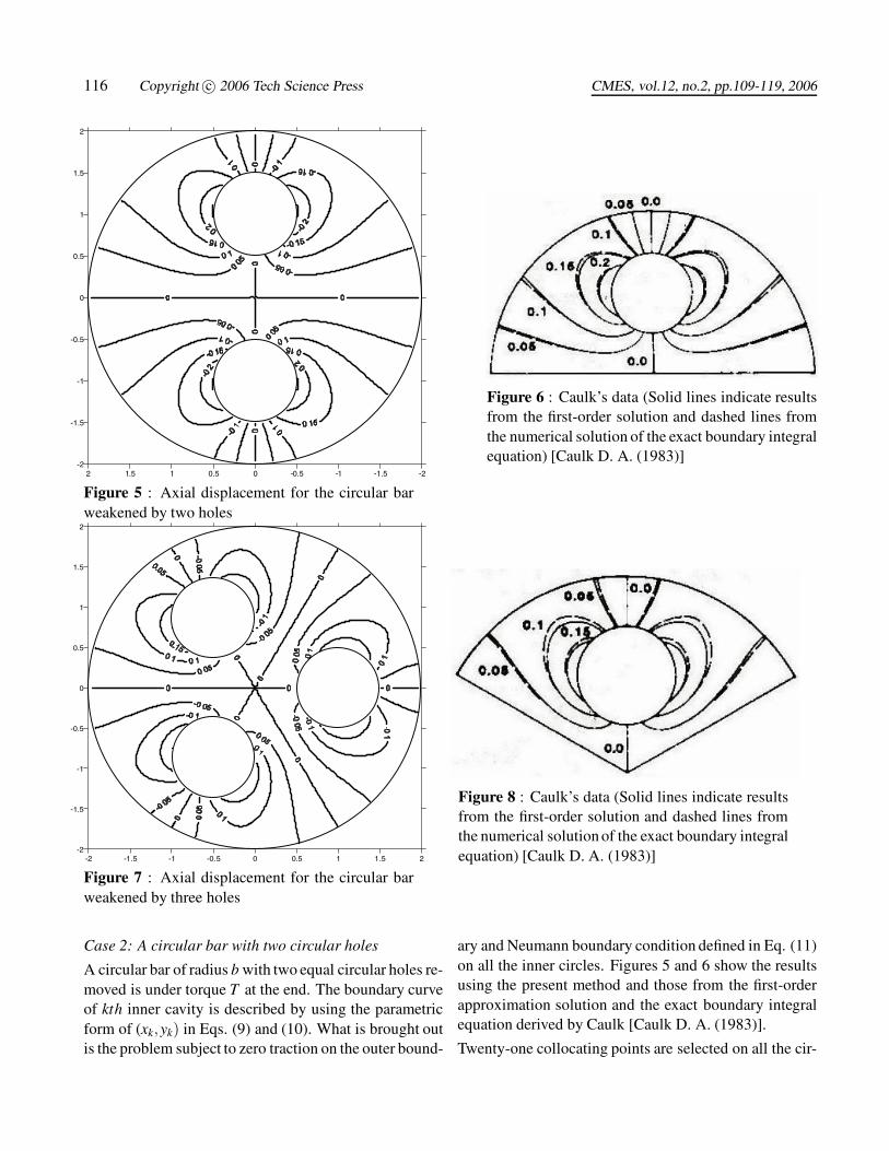
Figure 5 : Axial displacement for the circular barweakened by two holes

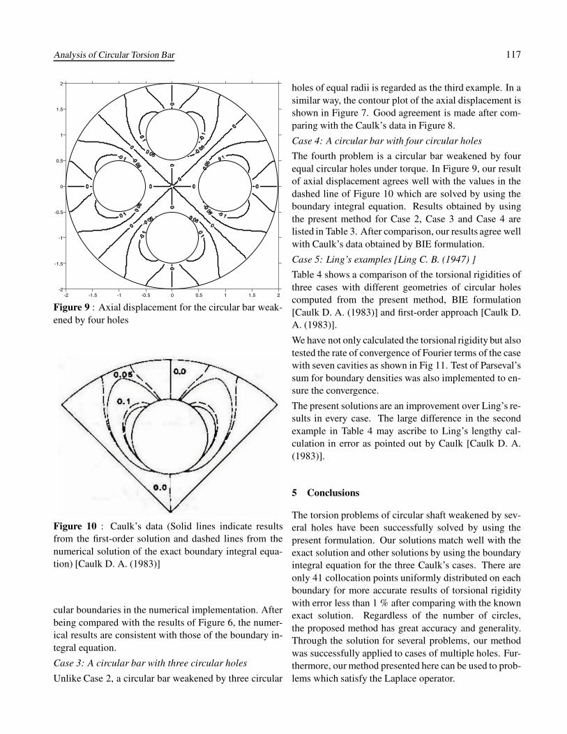
Figure 6 : Caulk’s data (Solid lines indicate resultsfrom the first-order solution and dashed lines fromthe numerical solution of the exact boundary integralequation) [Caulk D. A. (1983)]

-2 -1.5 -1 -0.5 0 0.5 1 1.5 2-2

-1.5

-1

-0.5

0

0.5

1

1.5

2

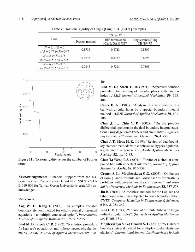
Figure 7 : Axial displacement for the circular barweakened by three holes

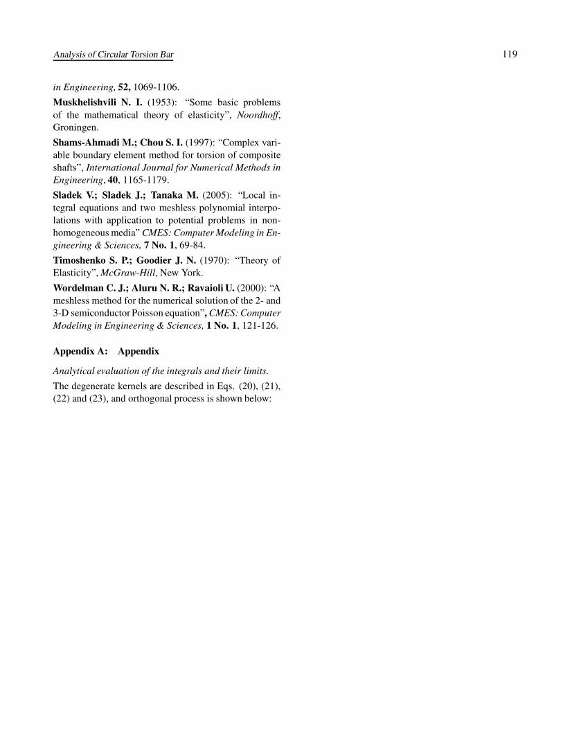
Figure 8 : Caulk’s data (Solid lines indicate resultsfrom the first-order solution and dashed lines fromthe numerical solution of the exact boundary integralequation) [Caulk D. A. (1983)]

Case 2: A circular bar with two circular holes

A circular bar of radius b with two equal circular holes re-moved is under torque T at the end. The boundary curveof kth inner cavity is described by using the parametricform of (xk,yk) in Eqs. (9) and (10). What is brought outis the problem subject to zero traction on the outer bound-

ary and Neumann boundary condition defined in Eq. (11)on all the inner circles. Figures 5 and 6 show the resultsusing the present method and those from the first-orderapproximation solution and the exact boundary integralequation derived by Caulk [Caulk D. A. (1983)].

Twenty-one collocating points are selected on all the cir-

Analysis of Circular Torsion Bar 117

-2 -1.5 -1 -0.5 0 0.5 1 1.5 2-2

-1.5

-1

-0.5

0

0.5

1

1.5

2

Figure 9 : Axial displacement for the circular bar weak-ened by four holes

Figure 10 : Caulk’s data (Solid lines indicate resultsfrom the first-order solution and dashed lines from thenumerical solution of the exact boundary integral equa-tion) [Caulk D. A. (1983)]

cular boundaries in the numerical implementation. Afterbeing compared with the results of Figure 6, the numer-ical results are consistent with those of the boundary in-tegral equation.

Case 3: A circular bar with three circular holes

Unlike Case 2, a circular bar weakened by three circular

holes of equal radii is regarded as the third example. In asimilar way, the contour plot of the axial displacement isshown in Figure 7. Good agreement is made after com-paring with the Caulk’s data in Figure 8.

Case 4: A circular bar with four circular holes

The fourth problem is a circular bar weakened by fourequal circular holes under torque. In Figure 9, our resultof axial displacement agrees well with the values in thedashed line of Figure 10 which are solved by using theboundary integral equation. Results obtained by usingthe present method for Case 2, Case 3 and Case 4 arelisted in Table 3. After comparison, our results agree wellwith Caulk’s data obtained by BIE formulation.

Case 5: Ling’s examples [Ling C. B. (1947) ]

Table 4 shows a comparison of the torsional rigidities ofthree cases with different geometries of circular holescomputed from the present method, BIE formulation[Caulk D. A. (1983)] and first-order approach [Caulk D.A. (1983)].

We have not only calculated the torsional rigidity but alsotested the rate of convergence of Fourier terms of the casewith seven cavities as shown in Fig 11. Test of Parseval’ssum for boundary densities was also implemented to en-sure the convergence.

The present solutions are an improvement over Ling’s re-sults in every case. The large difference in the secondexample in Table 4 may ascribe to Ling’s lengthy cal-culation in error as pointed out by Caulk [Caulk D. A.(1983)].

5 Conclusions

The torsion problems of circular shaft weakened by sev-eral holes have been successfully solved by using thepresent formulation. Our solutions match well with theexact solution and other solutions by using the boundaryintegral equation for the three Caulk’s cases. There areonly 41 collocation points uniformly distributed on eachboundary for more accurate results of torsional rigiditywith error less than 1 % after comparing with the knownexact solution. Regardless of the number of circles,the proposed method has great accuracy and generality.Through the solution for several problems, our methodwas successfully applied to cases of multiple holes. Fur-thermore, our method presented here can be used to prob-lems which satisfy the Laplace operator.

118 Copyright c© 2006 Tech Science Press CMES, vol.12, no.2, pp.109-119, 2006

Table 4 : Torsional rigidity of Ling’s [Ling C. B. (1947) ] examples

0 10 20 30 40

Fourier terms

0.724

0.725

0.726

0.727

0.728

0.729

tors

ion

al r

igid

ity

Figure 11 : Torsion rigidity versus the number of Fourierterms

Acknowledgement: Financial support from the Na-tional Science Council under Grant No. NSC91-2211-E-019-009 for Taiwan Ocean University is gratefully ac-knowledged.

References

Ang W. T.; Kang I. (2000): “A complex variableboundary element method for elliptic partial differentialequations in a multiply-connected region”, InternationalJournal of Computer Mathematics, 75, 515-525.

Bird M. D.; Steele C. R. (1992): “A solution procedurefor Laplace’s equation on multiple connected circular do-mains”, ASME Journal of Applied Mechanics, 59, 398-

404.

Bird M. D.; Steele C. R. (1991): “Separated solutionprocedure for bending of circular plates with circularholes”, ASME Journal of Applied Mechanics, 59, 398-404.

Caulk D. A. (1983): “Analysis of elastic torsion in abar with circular holes by a special boundary integralmethod”, ASME Journal of Applied Mechanics, 50, 101-108.

Chen J. T.; Chiu Y. P. (2002): “On the pseudo-differential operators in the dual boundary integral equa-tions using degenerate kernels and circulants”, Engineer-ing Analysis with Boundary Elements, 26, 41-53.

Chen J. T.; Hong H. K. (1999): “Review of dual bound-ary element methods with emphasis on hypersingular in-tegrals and divergent series”, ASME Applied MechanicsReviews, 52, pp. 17-33.

Chen T.; Weng I. S. (2001): “Torsion of a circular com-pound bar with imperfect interface”, Journal of AppliedMechanics, ASME, 68, 955-958.

Crouch S. L.; Mogilevskaya S .G. (2003): “On the useof Somigliana’s formula and Fourier series for elasticityproblems with circular boundaries”, International Jour-nal for Numerical Methods in Engineering, 58, 537-578.

Jin B. (2004): “A meshless method for the Laplace andbiharmonic equations subjected to noisy boundary data”,CMES: Computer Modeling in Engineering & Sciences,6 No. 3, 253-262.

Ling C. B. (1947): “Torsion of a circular tube with longi-tudinal circular holes”, Quarterly of Applied Mathemat-ics, 5, 168-181.

Mogilevskaya S. G.; Crouch S. L. (2001): “A Galerkinboundary integral method for multiple circular elastic in-clusions”, International Journal for Numerical Methods

Analysis of Circular Torsion Bar 119

in Engineering, 52, 1069-1106.

Muskhelishvili N. I. (1953): “Some basic problemsof the mathematical theory of elasticity”, Noordhoff,Groningen.

Shams-Ahmadi M.; Chou S. I. (1997): “Complex vari-able boundary element method for torsion of compositeshafts”, International Journal for Numerical Methods inEngineering, 40, 1165-1179.

Sladek V.; Sladek J.; Tanaka M. (2005): “Local in-tegral equations and two meshless polynomial interpo-lations with application to potential problems in non-homogeneous media” CMES: Computer Modeling in En-gineering & Sciences, 7 No. 1, 69-84.

Timoshenko S. P.; Goodier J. N. (1970): “Theory ofElasticity”, McGraw-Hill, New York.

Wordelman C. J.; Aluru N. R.; Ravaioli U. (2000): “Ameshless method for the numerical solution of the 2- and3-D semiconductor Poisson equation”, CMES: ComputerModeling in Engineering & Sciences, 1 No. 1, 121-126.

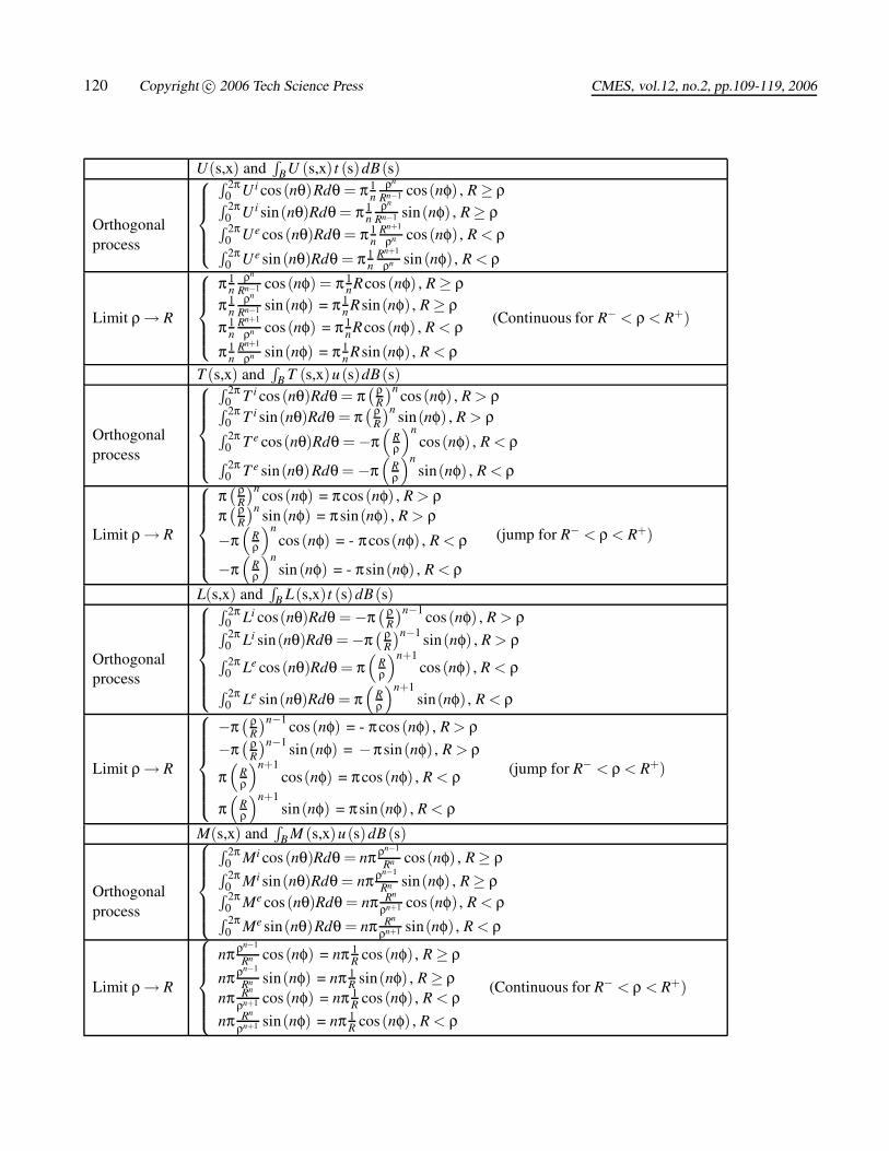
Appendix A: Appendix

Analytical evaluation of the integrals and their limits.

The degenerate kernels are described in Eqs. (20), (21),(22) and (23), and orthogonal process is shown below:

120 Copyright c© 2006 Tech Science Press CMES, vol.12, no.2, pp.109-119, 2006

U(s,x) andR

BU (s,x) t (s)dB(s)

Orthogonalprocess

⎧⎪⎪⎪⎨⎪⎪⎪⎩

R 2π0 Ui cos (nθ)Rdθ = π 1

nρn

Rn−1 cos(nφ) , R ≥ ρR 2π0 Ui sin(nθ)Rdθ = π 1

nρn

Rn−1 sin(nφ) , R ≥ ρR 2π0 Ue cos (nθ)Rdθ = π 1

nRn+1

ρn cos (nφ) , R < ρR 2π0 Ue sin(nθ)Rdθ = π 1

nRn+1

ρn sin(nφ) , R < ρ

Limit ρ → R

⎧⎪⎪⎪⎨⎪⎪⎪⎩

π 1n

ρn

Rn−1 cos (nφ) = π 1nRcos (nφ) , R ≥ ρ

π 1n

ρn

Rn−1 sin(nφ) = π 1n Rsin(nφ) , R ≥ ρ

π 1n

Rn+1

ρn cos (nφ) = π 1nRcos (nφ) , R < ρ

π 1n

Rn+1

ρn sin(nφ) = π 1n Rsin(nφ) , R < ρ

(Continuous for R− < ρ < R+)

T (s,x) andR

B T (s,x)u(s)dB(s)

Orthogonalprocess

⎧⎪⎪⎪⎪⎨⎪⎪⎪⎪⎩

R 2π0 T i cos (nθ)Rdθ = π

(ρR

)ncos (nφ) , R > ρR 2π

0 T i sin(nθ)Rdθ = π( ρ

R

)nsin(nφ) , R > ρR 2π

0 T e cos(nθ)Rdθ = −π(

Rρ

)ncos(nφ) , R < ρ

R 2π0 T e sin(nθ)Rdθ = −π

(Rρ

)nsin(nφ) , R < ρ

Limit ρ → R

⎧⎪⎪⎪⎪⎨⎪⎪⎪⎪⎩

π( ρ

R

)ncos(nφ) = πcos (nφ) , R > ρ

π( ρ

R

)nsin(nφ) = πsin(nφ) , R > ρ

−π(

Rρ

)ncos (nφ) = - πcos(nφ) , R < ρ

−π(

Rρ

)nsin(nφ) = - πsin(nφ) , R < ρ

(jump for R− < ρ < R+)

L(s,x) andR

B L(s,x)t (s)dB(s)

Orthogonalprocess

⎧⎪⎪⎪⎪⎪⎨⎪⎪⎪⎪⎪⎩

R 2π0 Li cos(nθ)Rdθ = −π

( ρR

)n−1 cos (nφ) , R > ρR 2π0 Li sin(nθ)Rdθ = −π

( ρR

)n−1 sin(nφ) , R > ρR 2π0 Le cos (nθ)Rdθ = π

(Rρ

)n+1cos (nφ) , R < ρ

R 2π0 Le sin(nθ)Rdθ = π

(Rρ

)n+1sin(nφ) , R < ρ

Limit ρ → R

⎧⎪⎪⎪⎪⎪⎨⎪⎪⎪⎪⎪⎩

−π( ρ

R

)n−1 cos (nφ) = - πcos (nφ) , R > ρ−π

( ρR

)n−1 sin(nφ) = −πsin(nφ) , R > ρ

π(

Rρ

)n+1cos(nφ) = πcos (nφ) , R < ρ

π(

Rρ

)n+1sin(nφ) = πsin(nφ) , R < ρ

(jump for R− < ρ < R+)

M(s,x) andR

B M (s,x)u(s)dB(s)

Orthogonalprocess

⎧⎪⎪⎪⎪⎨⎪⎪⎪⎪⎩

R 2π0 Mi cos (nθ)Rdθ = nπ ρn−1

Rn cos(nφ) , R ≥ ρR 2π0 Mi sin(nθ)Rdθ = nπ ρn−1

Rn sin(nφ) , R ≥ ρR 2π0 Me cos (nθ)Rdθ = nπ Rn

ρn+1 cos (nφ) , R < ρR 2π0 Me sin(nθ)Rdθ = nπ Rn

ρn+1 sin(nφ) , R < ρ

Limit ρ → R

⎧⎪⎪⎪⎪⎨⎪⎪⎪⎪⎩

nπ ρn−1

Rn cos (nφ) = nπ 1R cos (nφ) , R ≥ ρ

nπ ρn−1

Rn sin(nφ) = nπ 1R sin(nφ) , R ≥ ρ

nπ Rn

ρn+1 cos (nφ) = nπ 1R cos (nφ) , R < ρ

nπ Rn

ρn+1 sin(nφ) = nπ 1R cos (nφ) , R < ρ

(Continuous for R− < ρ < R+)