Analysis of Bathymetric Surveys to Identify Coastal Vulnerabilities at Cape Canaveral, FloridaBy David M. Thompson, Nathaniel G. Plant, and Mark E. Hansen

Open-File Report 2015–1180

U.S. Department of the InteriorU.S. Geological Survey

ii

U.S. Department of the InteriorSALLY JEWELL, Secretary

U.S. Geological SurveySuzette M. Kimball, Acting Director

U.S. Geological Survey, Reston, Virginia: 2015

For more information on the USGS—the Federal source for science about the Earth, its natural and living resources, natural hazards, and the environment—visit http://www.usgs.gov/ or call 1–888–ASK–USGS (1–888–275–8747).

For an overview of USGS information products, including maps, imagery, and publications, visit http://www.usgs.gov/pubprod/.

Any use of trade, firm, or product names is for descriptive purposes only and does not imply endorsement by the U.S. Government.

Although this information product, for the most part, is in the public domain, it also may contain copyrighted materials as noted in the text. Permission to reproduce copyrighted items must be secured from the copyright owner.

Suggested citation: Thompson, D.M., Plant, N.G., and Hansen, M.E., 2015, Analysis of bathymetric surveys to identify coastal vulnerabilities at Cape Canaveral, Florida: U.S. Geological Survey Open–File Report 2015–1180, 24 p., http://dx.doi.org/10.3133/ofr20151180.

ISSN 2331-1258 (online)

iii

AcknowledgmentsThe authors thank Trevor Browning, Tim Nelson, Rudy Troche, Christine Kranenburg,

Chris Pali, Calvin Peacock, Emily Klipp, Karen Morgan, Wayne Wright, and Chris Reich for supporting the 2014 data collection. Keitha Dattillo-Bain, Cheryl Hapke, and Jennifer Miselis reviewed the report, improved its clarity, and identified where additional insights could be extracted from this analysis.

iv

ContentsAcknowledgments ........................................................................................................................................................................................... iiiIntroduction ..................................................................................................................................................................................................... 1Methods ........................................................................................................................................................................................................... 1

Data Acquisition and Processing in 2014 .................................................................................................................................................... 2Sonar Based Acquisition Systems .......................................................................................................................................................... 2

GPS Navigation and Control .............................................................................................................................................................. 3Kinematic GPS Processing ................................................................................................................................................................ 5Kinematic Quality Control ................................................................................................................................................................... 5Bathymetric Processing...................................................................................................................................................................... 6

Lidar Acquisition System......................................................................................................................................................................... 6Sonar-Lidar Data Integration Methods.................................................................................................................................................... 6

Bathymetric Change Analysis .................................................................................................................................................................... 7Results ............................................................................................................................................................................................................. 9

Sonar Bathymetry Collected in 2014........................................................................................................................................................... 9Vertical and Horizontal Accuracies of Sonar Data Collected in 2014 ................................................................................................... 10

Lidar Bathymetry ........................................................................................................................................................................................11Vertical Accuracies.................................................................................................................................................................................11

Integrated Sonar and Lidar Bathymetry .....................................................................................................................................................11Bathymetric Change Analysis ................................................................................................................................................................... 13

Discussion and Conclusions .......................................................................................................................................................................... 19Implications of the Changes in Water Depth ............................................................................................................................................. 19Implications for Shoreline Change ............................................................................................................................................................ 20

References Cited .......................................................................................................................................................................................... 22Appendix I—Secchi Disk Observations ......................................................................................................................................................... 24

v

Figures1. Map of study area showing planned sonar survey track lines and outline of region mapped by lidar ............................................ 32. Stern view of Mako showing the PC, GPS antenna, TSS motion sensor, and fathometer transducer ........................................... 43. PC monitor and keyboard, forward of the operator, and box housing electronics on the stern of PWC; stern view of PWC

showing GPS antenna and transducer; and interior of electronics box with Echotrac CV100, PC, and Proflex GPS receiver ...... 44. Historical coverage: 1956 NOAA NOS sounding data; 2006 and 2007 NOAA NOS data; and 2010 USGS data .......................... 85. Historical coverage: 1956; 2006 and 2007 NOAA NOS data combined with the 2010 USGS data ............................................... 86. Sonar data collected on August 19 and 20, 2014. .......................................................................................................................... 97. Track line crossings ...................................................................................................................................................................... 108. Lidar data collected on August 19 and 20, 2014; and Secchi depths. .......................................................................................... 129. Comparison of lidar and sonar depths showing depth dependent bias of the lidar data. ............................................................. 1210. 2014 Lidar and sonar data points, and integrated sonar and lidar bathymetry ............................................................................. 1311. Bathymetry grids for the three datasets: 1956; combined 2006, 2007, and 2010 data; and 2014 integrated sonar and

lidar data ....................................................................................................................................................................................... 1512. Change in sea-floor elevation from 1956 to 2014; and change from the combined 2006/2007/2010 data to 2014 ..................... 1513. Profiles 1–3, Profiles 4–6, and Profiles 7–9 for 1956, 2010, and 2014 ......................................................................................... 1614. Gridded 1956 data; long-term bathymetric change; and gridded 2014 integrated sonar and lidar data ....................................... 1915. Gridded 2006/2007/2010 data; short-term bathymetric change (2006/2007/2010 to 2014); and gridded 2014 integrated

sonar and lidar data ...................................................................................................................................................................... 2116. Comparisons of patterns of erosion and deposition to cross-shore averaged depth changes, and short-term and long-term

shoreline change rates ................................................................................................................................................................. 21

Tables1. Track line crossing mean differences and standard deviations, in meters ....................................................................................11

vi

Conversion FactorsInternational System of Units to Inch/Pound

Multiply By To obtainLength

centimeter (cm) 0.3937 inch (in.)

millimeter (mm) 0.03937 inch (in.)

meter (m) 3.281 foot (ft)

kilometer (km) 0.6214 mile (mi)

Ratemeter per year (m/yr) 3.281 foot per year ft/yr)

Inch/Pound to International System of Units

Multiply By To obtainLength

inch (in.) 2.54 centimeter (cm)

foot (ft) 0.3048 meter (m)

mile (mi) 1.609 kilometer (km)

Ratefoot per year (ft/yr) 0.3048 meter per year (m/yr)

DatumVertical coordinate information is referenced to the North American Vertical Datum of 1988 (NAVD 88).Horizontal coordinate information is referenced to the North American Datum of 1983 (NAD 83).

AbbreviationsALPS Airborne Lidar Processing System

CORS Continuously Operating Reference Station

CTD conductivity, temperature and depth

GPS global positioning system

HTDP Horizontal Time-Dependent Positioning

IMU inertial measurement unit

NASA National Aeronautics and Space Administration

NGS National Geodetic Survey

NOAA National Oceanic and Atmospheric Administration

NOS National Ocean Service

NSE normalized squared error

OPUS Online Positioning User Service

PWC personal watercraft

RMS root mean square

RMSE root mean squared error

SANDS System for Accurate Nearshore Depth Surveying

U.S. United States

USGS U.S. Geological Survey

1

Analysis of Bathymetric Surveys to Identify Coastal Vulnerabilities at Cape Canaveral, FloridaBy David M. Thompson, Nathaniel G. Plant, and Mark E. Hansen

Introduction Cape Canaveral, Florida, is a prominent feature along the Southeast U.S. coastline. The region

includes Merritt Island National Wildlife Refuge, Cape Canaveral Air Force Station, NASA’s Kennedy Space Center, and a large portion of Canaveral National Seashore. The actual promontory of the modern Cape falls within the jurisdictional boundaries of Cape Canaveral Air Force Station. Erosion hazards result from winter and tropical storms, changes in sand resources, sediment budgets, and sea-level rise. Previous work by the USGS has focused on the vulnerability of the dunes to storms, where updated bathymetry and topography (Bonisteel-Cormier and others, 2011) have been used for modeling efforts (Stockdon and others, 2013). Existing research indicates that submerged shoals, ridges, and sandbars af-fect patterns of wave refraction and height, coastal currents, and control sediment transport (Trowbridge, 1995; Hulscher, 1996; Warner and others, 2014). These seabed anomalies indicate the availability and movement of sand within the nearshore environment, which may be directly related to the stability of the Cape Canaveral shoreline. Understanding the complex dynamics of the offshore bathymetry and as-sociated sediment pathways can help identify current and future erosion vulnerabilities due to short-term (for example, hurricane and other extreme storms) and long-term (for example, sea-level rise) hazards.

The purpose of this work is to describe an updated bathymetric dataset collected in 2014 (Han-sen and others, 2015) and compare it to previous datasets. The updated data focus on the bathymet-ric features and sediment transport pathways that connect the offshore regions to the shoreline and, therefore, are related to the protection of other portions of the coastal environment, such as dunes, that support infrastructure and ecosystems. Previous survey data include National Oceanic and Atmospheric Administration’s (NOAA) National Ocean Service (NOS) hydrographic survey from 1956 and a USGS survey from 2010 (Thompson and others, 2015) that is augmented with NOS surveys from 2006 and 2007. The primary result of this analysis is documentation and quantification of the nature and rates of bathymetric changes that are near (within about 2.5 km) the current Cape Canaveral shoreline and inter-pretation of the impact of these changes on future erosion vulnerability.

MethodsThe requirements for this effort are to compare a recent bathymetric dataset to prior datasets.

The updated bathymetry was collected during August 2014 (Hansen and others, 2015). These data were acquired using (1) single-beam sonar systems deployed from a motor boat and two personal water crafts (PWC) and (2) lidar collected with an airborne system. Raw data from each of these systems were col-lected and processed differently. Once collected, the data from the different systems were evaluated for errors and then integrated into a single dataset to be used in the comparison to prior data. This Methods section explains the data acquisition, processing, and analysis approaches.

2

Data Acquisition and Processing in 2014

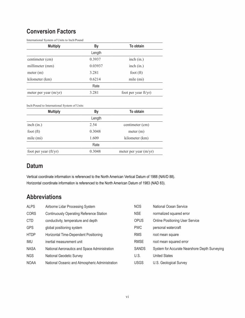
The USGS conducted a bathymetric mapping survey on August 19-20, 2014, in the Atlantic Ocean offshore from Cape Canaveral, FL. The study area extends from Port Canaveral, FL, to the northern end of NASA’s Kennedy Space Center property and from the shoreline to about 2.5 km off-shore. The planned survey track lines for the sonar collection were spaced 500 m apart in the alongshore direction and were made of varying lengths to allow for the survey to be completed in 2 days (fi g. 1). The data collected, along with historical data, will be analyzed on these track lines. The objective of this component of the survey was to (1) provide ground truth for the airborne lidar survey and (2) fill in data gaps where lidar data were not successfully acquired. Some track lines extended farther offshore to in-crease the sample coverage at (1) the north and south boundaries of the survey area and (2) some known shoals where shallow depths were expected farther from shore. The sonar operations were conducted in two missions, one on each day.

The lidar operations were conducted in three missions; one in the afternoon of August 19 and one each in the morning and afternoon of August 20. The lidar missions were synchronized with the sonar surveys such that there was some temporal overlap between the operations. Additional data were collected using a Secchi disk to evaluate the water clarity and relate it to the lidar’s ability to receive bathymetric returns. Wave breaking produces foam and bubbles, and sediment plumes are mobilized by waves and by wave-driven or tidal currents. For example, sediment plumes were observed near the entrance to Port Canaveral during ebb tides which reduced the effectiveness of the lidar system. Sonar systems were not affected by these conditions.

Sonar Based Acquisition Systems

The bathymetric survey was conducted offshore from Cape Canaveral, utilizing the global posi-tioning system (GPS)-based, single-beam sonar that is integrated to form a System for Accurate Near-shore Depth Surveying (SANDS; DeWitt and others, 2007). Two types of platforms were utilized for the survey, both equipped with variations of SANDS hardware. One platform was a 17-ft Mako outboard motor boat equipped with a precision GPS receiver, motion compensator, and survey grade fathometer. The second type of platform was a Yamaha WaveRunner PWC equipped with a precision GPS receiver and survey grade fathometer. Two PWCs were simultaneously operated for the survey. The Mako also acted as a support vessel for the PWCs in the event of any electrical or mechanical failures.

The Mako system used an Ashtech® Z-Extreme™ GPS receiver with Dorne/Margolin choke ring antenna on the boat (fig. 2). The PWCs used a Proflex™ 800 CORS GPS receiver and an Ashtech® geodetic survey antenna (fig. 3). Water depth measurements on all three vessels were recorded at 10Hz with an ODOM Echotrac CV100 echo sounder using 200 kilohertz (kHz) transducers. Boat motion on the Mako (heave, pitch, and roll) was recorded at 20Hz using a TSS DMS-05 sensor. Due to the antenna configuration, a motion compensator was neither necessary nor used on the PWCs. Data from all on-board sensors were recorded on Microsoft Windows PCs using HYPACK, Inc. HYPACK® software.

Variable water densities through the water column affect the travel speed of sound thus influ-encing the measured water depth. To correct for varying water densities, speed of sound measurements through the water column were collected using a SonTek Castaway conductivity, temperature, and depth (CTD) probe. Several casts were collected each survey day at varying times and locations.

3

GPS Navigation and Control

The type of navigation used for this project employed kinematic full-carrier phase differen-tial GPS processing. This operation utilized a reference GPS receiver located on a fixed and precisely known location and a rover (aircraft/boat) GPS receiver that recorded survey positions. Processing the full-carrier phase data allows very precise positioning of the reference and rover receivers. Differential processing improves the rover positions by assessing positional errors computed at the reference re-ceiver and applying those errors or differences to the rover receiver.

For this survey, a National Geodetic Survey (NGS) Continuously Operating Reference Station (CORS) and a newly established USGS benchmark were used as survey control for both aircraft and boat surveys. The CORS station used is named “Cape Canaveral 6” and designated “CCV6.” The coordinates used for this station were extracted from the NGS coordinate sheet for “CCV6” and provided relative to the International GNSS Service reference frame (IGS08). The IGS08 coordinates for “CCV6” were trans-formed to WGS84 (G1150) using the NGS Horizontal Time-Dependent Positioning (HTDP) software

Figure 1. Map of study area showing planned sonar survey track lines (red) and outline (blue) of region mapped by lidar.

4

Figure 3. (A) PC monitor and keyboard, forward of the operator, and box housing electronics on the stern of PWC. (B) Stern view of PWC showing GPS antenna and transducer. (C) Interior of electronics box with Echotrac CV100, PC, and Proflex GPS receiver. Photograph by USGS.

Figure 2. (A) Stern view of Mako showing the PC, GPS antenna, TSS motion sensor, and fathometer transducer. Note that the transducer mount rotates and is shown in the upright position for transit. (B) Inte-rior of electronics box showing Echotrac CV100 and Z-Extreme GPS receiver. Photograph by USGS.

5

version 3.2.3. The newly established USGS benchmark was located at Space Coast Regional Airport and designated “KTIX.” This reference station was created to better initialize aircraft GPS data prior to and after survey flight missions. Since this was a new location, precise coordinates needed to be determined in order for this station to be used as a GPS reference station. The USGS has developed a method for es-tablishing new bench marks. It should be noted that this method conforms to NGS “Blue Book” standards and internal tests conducted by the USGS indicate this method is accurate to +/– 2 cm (D. McDonald, 2002). For “KTIX,” a PK nail (hardened 3-in. survey nail made by Parker Kaelon) was driven into the tarmac surface until resistance was met. The reference GPS antenna was then placed on the PK nail for data collection. The new benchmark was occupied by the reference GPS receiver for a minimum of three 8-hour occupations recorded at a minimum of 30-second epoch intervals. The autonomous static GPS processing software service, NGS’s Online Positioning User Service (OPUS) version 1.95, was used to compute new benchmark coordinates for each daily occupation. OPUS uses the nearest three CORS sta-tions. The stated vertical accuracies of OPUS is between 0.4 to 1 in. (1 to 3 cm) root mean square (RMS). OPUS coordinates are provided in IGS08 horizontal coordinates and ellipsoid height vertical coordinates. For this survey, HTDP software version 3.2.3 was used to convert IGS08 to WGS84 (G1150) coordinates. Positions derived from all occupations were then averaged after outliers were removed. Positions with differences greater than 2 standard deviations from the mean were considered outliers. The derived posi-tion was then used to process the appropriate kinematic aircraft and boat data.

Kinematic GPS Processing

Precise aircraft and boat trajectories were determined using the full-carrier phase differential GPS data and Novatel/Waypoint GrafNav software version 8.5. GrafNav calculates the relative position of the aircraft/boat receiver to the base receiver. Thus, all trajectories are relative to the reference station position which is the rationale for the involved determination of reference station coordinates. A single output file of precise aircraft/boat trajectory, and quality control information at 0.1 second intervals was produced for each survey day for each survey platform. The output provides precise position measure-ments that are time stamped with GPS time. These trajectory data are later merged with the mapping sensor and motion data collected on board the aircraft/boat.

Kinematic Quality Control

GrafNav offers forward and backward time series processing which is the preferred tool to as-sess trajectory quality. Each time series is an independent calculation of the trajectory. In theory, each time series should produce the same position for each epoch. Since GrafNav uses various filters and po-sition estimators, there are often differences within each time series. An estimation of the data accuracy can be assessed by differencing the two time series, referred to a position separation. In general, a verti-cal separation of 10 cm is considered acceptable with a difference of less than 5 cm considered to be exceptionally good and is implied that this separation is the vertical GPS measurement error. The GPS data are processed with various options until these criteria are met. Due to the signal geometry, it can be assumed the horizontal measurement error is one-half the vertical error. For this dataset, the maximum vertical separation was 12 cm.

6

Bathymetric Processing

Post-processing of the sonar data was accomplished with algorithms written by USGS scientists using the MathWorks MATLAB computing environment. The processing software is used to edit erro-neous sounding data, synchronize the precise boat GPS trajectory with sonar data, and apply geometric corrections using the recorded pitch and roll measurements (Mako only). The final processing step cre-ates sea-floor elevations by merging the measured distance from the ellipsoid to the GPS antenna phase center, corrected GPS/transducer staff height, and corrected distance from the transducer to the sea floor. Thus, final elevations are relative to the ellipsoid (WGS84). A speed of sound correction (Fofonoff and Millard, 1983) is then applied to the sounding data. Since the CTD data showed very little spatial and temporal variation, daily mean values of the CTD data were used for this correction.

Lidar Acquisition System

The EAARL-B is an airborne lidar that includes a raster-scanning, water-penetrating, full-wave-form, adaptive lidar and an array of precision kinematic GPS receivers, which provide for submeter geo-referencing of each laser sample (Wright, 2013). EAARL-B detects, captures, and automatically adapts to each laser return backscatter over a large signal dynamic range. Optical clarity was measured using a 19.75 cm diameter Secchi disk, cast overboard from the support boat (Mako) while drifting. The disk was lowered to the point where it was not visible or to the sea floor if visibility exceeded the water depth. When the sonar fathometer was running, the measured water depth was included in the observa-tion. In one case the current pulled the disk away from vertical, and a Secchi depth was recorded that exceeded the water depth.

Post-processing of EAARL-B data is accomplished using the Airborne Lidar Processing System (ALPS), (Bonisteel and others, 2009; Nayegandhi and others, 2009) that combines laser return backscat-ter digitized at 1-ns (nanosecond) intervals with aircraft positioning data derived from the inertial mea-surement unit (IMU) and GPS receivers. ALPS was used to detect the first return from the water (or land for topographic surveys) surface as well as to find a last return corresponding to the sea floor. In sub-merged environments, effects of refraction and change in speed of light as it enters the water column are accounted for a “submerged topography” algorithm. The lidar data were reviewed manually, and data that obviously did not penetrate to the sea floor were removed on the basis of experience by an expert analyst. The equivalents of dE (delta Ellipsoid), dS (delta Staff), dB (delta Bed) are computed and used to determine the final elevations of the submerged topography relative to the ellipsoid (WGS84).

Sonar-Lidar Data Integration Methods

The high spatial resolution (several points per square meter in shallow water) of the lidar data provides the best estimates of bathymetric elevations and elevation variability associated with the pleth-ora of bars, shoals, and ripples that were not resolved by relatively coarse alongshore spacing (500 m) of the boat-based surveys that were conducted along cross-shore transects (fig. 1). Where the water clarity was not sufficient to allow lidar penetration to the sea floor, however, the sonar data were needed to fill gaps in data coverage. Therefore, a weighting scheme to combine the two sample methods is employed, utilizing lidar where possible and blending it with the sonar where necessary.

The scheme involves interpolation that filters some small-scale detail and ensures that the larg-est-scale features, with lengths of 100s to 1,000s of meters, are resolved and, if there are insufficient data, the uncertainty in the resulting interpolated bathymetry is tracked. The interpolation method uses

7

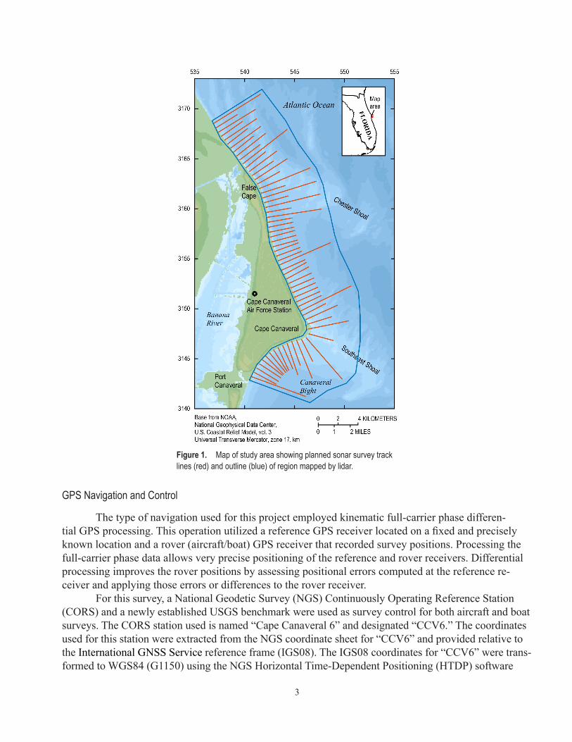
a grid-based approach with smoothing scales that adapt to the grid resolution (Plant and others, 2002; Plant and others, 2009). We used different interpolation filters for the sonar and lidar data, and data were extracted at a resolution of 125 m in the alongshore direction and 10 m in the cross-shore direction. This resolution is not satisfied by the sonar data sampling strategy, so these data were smoothed over 500 m to span the alongshore sample spacing and smoothed over 20 m in the cross-shore direction. Lidar data were smoothed over 125 m in the alongshore direction and over 20 m in the cross-shore direction.

The interpolation results produce two datasets (one for lidar and one for sonar) that include a smooth interpolation grid plus error fields that include (1) the root mean square error (RMSE) of the data compared to the smooth interpolation and (2) the normalized sampling error (NSE) that quantifies how well the sample data satisfied the grid resolution. If sample data did not satisfy the grid resolution, the NSE is nearly 1, indicating that the interpolation did not succeed in filtering short-scale variability or random errors. On the other hand, if the sample data were very dense, the NSE is close to zero, indicat-ing that the interpolation removed all sub-grid scale variability. In general, the lidar data will have a very low NSE (unless the water clarity is poor), and the sonar data will have a higher NSE. For each dataset, within a grid cell data with extremely high variability or extremely poor sampling are rejected using threshold values of RMSE>20 cm NSE>0.5, respectively. This supports a weighting scheme to blend the two datasets:

ZA = ZS +W ZL − ZS( ) ,

where ZA is the assimilated bathymetry result, ZS is the interpolated sonar bathymetry, and ZL is the inter-polated lidar bathymetry. The assimilation weight, W, is computed as:

W = NSES / NSEL + NSES( ) ,where the NSE for sonar and lidar are compared and, for instance, if NSES is larger than NSEL, W will be close to 1 and the assimilated value will be equal to the interpolated lidar value, ZL. Otherwise, the two inputs are combined in a weighted sum. Finally, the quality of the assimilation is reported as an effective NSE:

NSEA = NSES 1−W( ) .Hence, NSEA reflects how much the lidar data reduce the error in the sonar data.

Bathymetric Change Analysis

For analyzing bathymetric change, NOAA NOS surveys of the Cape Canaveral area were ob-tained from the NOAA Web site (http://www.ngdc.noaa.gov/mgg/bathymetry/relief.html, accessed 04/01/2015) and also utilized a 2010 USGS survey (fig. 4C). Three surveys were completed by NOAA in 1956, the combination of which covered the entire Cape Canaveral region (fig. 4A). A survey was also completed by NOAA in the spring of 2006 covering the Canaveral Bight area and a survey was conducted in the summer of 2007 covering the Southeast Shoal area (fig. 4B). For the bathymetric change analysis, the data from 1956 were used to identify historical changes over a long time interval, and the NOAA 2006 and 2007 data were combined with the USGS 2010 data to identify recent changes (fig. 5B). The combination of the more recent 2006, 2007, and 2010 data provides a nearly complete coverage of the study area over this 4-year period. All sounding data were converted to the NAVD88 datum using NOAA’s VDatum software. The NAVD88 datum yields depths that are referenced to a value that is approximately mean sea level.

8

Figure 4. Historical coverage: (A) The 1956 NOAA NOS sounding data. (B) The 2006 and 2007 NOAA NOS data (5/15/2006 – the dense data out of Port Canaveral and south of the Cape and 8/16/2007 – data over the Southeast Shoal). (C) The 2010 USGS data.

Figure 5. Historical coverage: (A) 1956. (B) The 2006 and 2007 NOAA NOS data combined with the 2010 USGS data.

9

ResultsThe results are presented in four sections. The first section describes the data collected by the

sonar systems. The second section describes the data collected by the lidar system. The third section de-scribes the integrated bathymetric dataset that utilized both sonar and lidar data. Both data descriptions include analysis of survey errors. The final section describes the bathymetric changes over the long-term period (1956 to 2014) and shorter-term period (2006 to 2014).

Sonar Bathymetry Collected in 2014

Sonar data were collected on all but two of the planned track lines (fig. 6). Both of the unsam-pled lines were at the Cape point and were neglected because wave shoaling presented unsafe boating conditions in the area during the survey. Additionally, two alongshore crossing lines along the entire North-South length of the study area were collected. These crossing lines, in addition to duplicated lines collected at the northern end of the study area, allowed for a crossing analysis to check for any bias er-rors among the sonar data collected by each vessel.

Figure 6. Sonar data collected on August 19 and 20, 2014.

10

Vertical and Horizontal Accuracies of Sonar Data Collected in 2014

Errors in the data from the three sonar systems were evaluated by comparing the bathymetric differences at track line crossings or along repeated track lines. Figure 7 shows all the line crossings between the three survey vessels, including cases where any one vessel crossed its own track. For ex-ample, points labeled “WVR1 WVR1” indicate where WaveRunner 1 crossed its own track. Recorded depths within a 1 m diameter circle of each intersection were analyzed for differences and are reported in table 1. In theory, the values at a crossing point should be the same, and any deviation represents er-rors due to system noise and possible biases if the systems are not perfectly calibrated. This technique only evaluates the relative accuracy of the survey, because all measurements are relative to the reference station coordinates, and assumes no bias with the reference station itself. This crossing analysis shows that the WaveRunners were self-consistent (note that the Mako did not cross itself). A small, 2 cm, bias

Figure 7. Track line crossings. The individual track lines for each vessel are shown as lines: black – WaveRunner 1, grey – WaveRun-ner 2, and white – Mako. The track line crossings of a vessel with itself and with other vessels are shown as colored circles.

11

was noted between the WaveRunners, and larger, 9 cm and 11 cm, biases were noted between the Mako and WaveRunner 1 and WaveRunner 2, respectively. Utilizing mean differences (μz) from this analysis, bias corrections were applied to the WVR1 and Mako data. After the bias correction was applied, the crossing analysis revealed that the vertical accuracy of the soundings, calculated as the mean absolute difference (σz), was 7 cm. The estimated horizontal accuracy derived from the GPS precise trajectory data and the reference station coordinates was 0.04 m RMS.

Table 1. Track line crossing mean differences (µz) and standard deviations (σz), in meters (m).

Boats Number of points µz (m) σz (m)WVR1 WVR1 416 -0.011 0.077

WVR2 WVR2 158 0.004 0.087

Mako Mako 0

WVR1 WVR2 834 0.021 0.070

WVR1 Mako 2,460 -0.095 0.093

WVR2 Mako 1,001 -0.112 0.092

Lidar Bathymetry

Lidar soundings were collected from the shoreline out to approximately 2 km offshore and from just south of Port Canaveral north past the north boundary of the Kennedy Space Center property (fig. 8). The areas with gaps in the data, as well as the lack of coverage south of the Cape, are areas where, due to optical clarity of the water, lidar was unable to penetrate the water column to the sea floor to get a valid depth reading. Using the Secchi disk data, it was found that lidar returns were obtained at depths that were 2.4 (±0.3) Secchi depths (fig. 8B).

Vertical Accuracies

To assess the vertical accuracy of the lidar bathymetry, the sonar and lidar data were interpolated to the planned sonar survey track lines as described in the “Sonar-Lidar Data Integration Methods” sec-tion. Offsets from the historical datasets can be calculated in the same way such that all data are treated objectively, regardless of differences in sampling density and patterns. Using the sonar data as “ground-truth” for the lidar data, the depths were compared (fig. 9) and a small (<10 percent) depth-dependent bias was found. This bias resulted in a mean offset of 0.27 cm and an RMS difference of 0.35 m. A bias correction was applied to the lidar data using a linear model that included a gain correction (0.944 times the sampled lidar depth) and an offset correction (0.172 m). The RMS difference between sonar and corrected lidar elevations was reduced to 0.17 m. The corrected lidar data were used in the analysis presented in this report.

Integrated Sonar and Lidar Bathymetry

The sonar and lidar sounding data collected in August 2014 were integrated as described in the “Sonar-Lidar Data Integration Methods” section. The result (fig. 10B) is a smooth set of interpolated depths that are evaluated on cross-shore transects spaced approximately 250 m apart in the alongshore direction. This result doubles the resolution that would have been obtained from the sonar survey alone and fills in gaps where turbidity prevented the lidar survey from detecting the sea floor. Some gaps re-

12

Figure 8. (A) Lidar data collected on August 19 and 20, 2014, and (B) Secchi depths.

Figure 9. Comparison of lidar and sonar depths showing depth dependent bias of the lidar data.

13

main where there were no lidar observations or sonar observations. These gaps do not impair our ability to identify large-scale features such as oblique sand ridges, shoals, and deep channels and depressions. These features and their connection to the area near the shoreline are expected to evolve through time and illustrate changes in nearshore morphology that might be indicative of changing sediment transport pathways.

Bathymetric Change Analysis

The updated bathymetry data were compared to previous datasets to estimate depth changes at two time scales. For longer-term changes, data were compared to a NOAA bathymetric survey from 1956. To constrain the time scales associated with long-term changes, the 2014 data were compared to the combined 2006–2010 data. This comparison identifies whether changes happened prior to 2006–2010 (depending on location), and it shows interannual variations where 2006–2010 data differ from 2014 data. The consistently interpolated gridded elevations of these datasets are shown in fi gure 11. Changes over the entire region (fig. 12) include significant erosion and deposition (>0.5 m, our thresh-old for significance based on our analysis of offset and sample error) over the longer time interval that are dominated by large-scale features. The interannual changes over the 2006–2014 period are relatively small, except near the shoreline and a few isolated patches throughout the study region. This suggests

Figure 10. (A) 2014 Lidar (red) and sonar (blue) data points, and (B) Integrated sonar and lidar bathymetry..

14

that much of the bathymetric change either occurred slowly or was associated with one or more events in the past. The patterns of bathymetric changes, which reflect both short-term and long-term coastal sediment processes, can be summarized as follows:

• In the region north of False Cape there are alternating patterns of erosion (red) and deposition (blue) that are associated with the migration of oblique sand ridges (fig. 12 A). The sand ridges extend from offshore (8 m depth) to the beach at the far north and intersect and interact with the shoal offshore from False Cape. The sand ridges have a length of about 2 km and a vertical height (trough to crest) of about 5 m. Alongshore transects (not shown) were used to estimate an alongshore migration rate of 5–6 m/yr toward the south. (The standard deviation of several migration-rate estimates was 1 m/yr.) In profile view along the cross-shore transects (fig. 13, Profiles 1 and 2), the migration of the oblique ridge results in deposition near the shore, where the ridge intersects the beach, and erosion upcoast from this point. Because the ridges are oblique to the coast, they also exhibit apparent cross-shore migration, which was estimated to be 2.6 m/yr (0.3 m/yr standard deviation).

• In the region including False Cape and Chester Shoal, there is erosion on the north side of Chester Shoal and deposition in the trough between the shore and the shoal (fig. 12 A). The elevation of the central part of Chester Shoal (fig. 13, Profile 3) is relatively stable, and changes appear to have inter-annual variability. Deposition on the shoreward flank of the shoal was more pronounced in the 2010 survey, indicating that there is substantial interannual variability here as sediment shifts from one location to another without significant gains and losses over the transect.

• In the mid-Cape region between False Cape and Cape Canaveral, there generally is erosion that is associated with volume loss as a broad shoal has developed into a series of oblique sand ridges. The ridges that developed are about 3 m high (trough to crest) and have alongshore lengths of 300 to 700 m. The complexity of these changes is better understood when looking at the historic and updated bathymetry maps along with the bathymetric change map (fig. 14). Examination of a cross section at this location (fig. 13, Profile 5) also shows erosion of the shoal that had already occurred by 2010. Another feature, the ridge connecting the Chester Shoal to the region near the shoreline, has been eroded and its crest has moved further offshore (fig. 13, Profile 4).

• In the south region, including Cape Canaveral, Southeast Shoal, and Canaveral Bight, the pattern of erosion from the mid-Cape region extends toward the axis of Southeast Shoal, and deposition occurs south of this area (fig. 14). In Canaveral Bight, there are alternating erosion patterns associated with the migration or formation of sand ridges (fig. 13, Profile 8). The changes were apparent by 2010, so these are considered long term, or at least they occurred prior to 2010 (or prior to 2006/2007). In this region, there is substantial deposition near the shoreline (fig. 13, Profiles 8 and 9).

• Finally, along the entire study area, the region near the shoreline shows persistent deposition. This deposition occurs in the shallow depths where rapid changes in elevation can occur. The changes are likely associated with passing storms, which can erode the beach and deposit sand in this shallow zone. However, the 2014 survey was conducted during a period when there were no storms, and this deposition could also reflect longer-term, persistent erosion of the subaerial beach.

15

Figure 12. (A) Change in sea-floor elevation from 1956 to 2014. (B) Change from the combined 2006/2007/2010 data to 2014.The black lines are transects where the profiles of the datasets are shown in figure 13.

Figure 11. Bathymetry grids for the three datasets: (A) 1956. (B) The combined 2006, 2007, and 2010 data. (C) The 2014 integrated sonar and lidar data.

16

Figure 13. Profiles 1–3. Blue – 1956, red – 2010, and yellow – 2014. Profile locations are shown in fi gure 12.

17

Figure 13—Continued. Profiles 4–6. Blue – 1956, red – 2010, and yellow – 2014. Profile locations are shown in fi gure 12.

18

Figure 13—Continued.. Profiles 7–9. Blue – 1956, red – 2010, and yellow – 2014. Profile locations are shown in fi gure 12.

19

Discussion and ConclusionsThe observed changes in depth over the long term (1956 to 2014) and the lack of change over

the short term (2010 to 2014) can be used to understand sediment transport processes, their time scales, and the implications for future vulnerability. Here, the changes described above in each of four regions (north of False Cape, False Cape, mid-Cape, and Cape Canaveral) are interpreted and related to shore-line change over the very long term (1900 to present) and shorter term (1970 to present—approximately consistent with the long-term period of our bathymetry analysis).

Implications of the Changes in Water Depth

• The migration of sand ridges that is most apparent in the north end of the study area can be used to quantify the net southward flow of sediment from the north to the Cape Canaveral coastline. These features are thought to be formed by steering of storm-driven currents and associated sediment trans-port patterns (Trowbridge, 1995). The southward sediment transport (and hence migration) of these ridges is expected if sediment transport is dominated by extratropical storms, the direction of which is consistent with conditions that are expected to maintain the ridges (Warner and others, 2014). Thus, the dependence on changes in storm climatology and interactions of storm processes with these sand features can alter the timing and magnitude of net sediment transport to the region.

• In the vicinity of False Cape, Chester Shoal appears to be changing shape slowly, with the shoal gen-erally migrating toward the south, at least in the area nearest the shoreline, and eroding offshore. The broad extent of this shoal is much larger than the sand ridges, some of which appear to be superim-posed on the shoal. The changes in the shoal are likely to affect wave-refraction patterns, which can ultimately alter erosion and accretion patterns near the shoreline. The change from erosion (mov-

Figure 14. (A) Gridded 1956 data. (B) Long-term bathymetric change (1956 to 2014). (C) Gridded 2014 integrated sonar and lidar data.

20

ing alongshore to the south, figs.12A and 16B) to accretion of the nearshore region at False Cape is likely due to the interaction of waves with Chester Shoal and other shoals that are farther offshore outside of the boundary of this study.

• The mid-Cape region to the south of False Cape appears to be eroding. This was not expected if it is assumed that net sediment transport to the south would drive net southward migration of Chester Shoal. By comparing the detailed features of Chester Shoal in the 1956 and 2014 bathymetries, it appears that the features themselves have been diminished. Recent analysis by Absalonsen and Dean (2010, fig. BRE-3) show net shoreline recession in the recent (1969–2008) period. In this region, there appears to be net erosion in the offshore region (for example, Profile 5, fig. 13) and, although there is some nearshore deposition here, it does not balance the erosion. And, the nearshore deposi-tion here may only reflect interannual phenomena as the profile to the immediate south (Profile 6, fig. 13) does not show the same nearshore deposition pattern over the short timescale (for example, the deposition was not apparent in 2006–2010).

• The Cape and Southeast Shoal section shows patterns of erosion and deposition that are consistent with southward migration of Cape Canaveral itself. The overall erosion of the mid-Cape section may be part of this migration pattern as the upcoast flank of Cape Canaveral erodes in order to supply sediment to the down coast flank of the cape. Deposition near the shoreline in the Canaveral Bight may be the end point for some of the eroded sediment; however, this study did not include a wide enough area to determine if there is a balance of erosion and deposition over the whole Cape Canav-eral coastal complex or whether there may be a net import or export of sediment.

Implications for Shoreline Change

The apparent nearshore deposition over much of the study region could simply indicate a short-term exchange of sediment between the beach and the surf zone due to past storms or it could indicate a longer-term trend in the distribution of sediment. It is well documented that there are regions of shore-line erosion and deposition (Morton and Miller, 2005; Absalonsen and Dean, 2011) along the Cape Ca-naveral coastline, and the data presented here can be used to relate shoreline change (and, specifically, erosion vulnerability) to patterns of erosion and deposition (fig. 16). This allows us to identify areas where the well-documented shoreline changes indicate sediment redistributions that are confined to the shoreline zone versus areas where shoreline changes are tied to much larger-scale bathymetric changes. On the basis of the long-term shoreline change data, the same four regions, as identified above, have dif-ferent characteristics:

• North of False Cape, long-term shoreline change is mildly erosional (change does not exceed 1 m/yr). Short-term shoreline change is variable and generally accretional except in the region where a sand ridge intersects the shoreline. The continued migration of the sand ridges is expected to move the area of impact to the south at a rate of about 5 m/yr. It is likely that the impact to the shoreline will occur at the long timescale associated with this migration as well as causing interannual varia-tions associated with interactions between the shore and the sand ridge under different wave condi-tions (McNinch, 2004; Schupp and others, 2006). The cross-shore averaged depth changes are not significantly different from zero, suggesting that shoreline vulnerabilities are not tied to net sediment losses across the nearshore region.

21

Figure 15. (A) Gridded 2006/2007/2010 data. (B) Short-term bathymetric change (2006/2007/2010 to 2014). (C) Gridded 2014 inte-grated sonar and lidar data.

Figure 16. Comparisons of patterns of (A) erosion (red) and deposition (blue) to (B) cross-shore averaged depth changes (μΔz is the average elevation change in meters, σΔz is the standard deviation) and short-term and long-term shoreline change rates (meters per year, from Morton and Miller, 2005).

22

• Immediately south of False Cape, long-term and short-term shoreline changes are accretional (ex-ceeding 1 m/yr). Although there is substantial depth-change variability in this area, the cross-shore averaged depth changes are not significantly different from zero. This suggests that some sort of balance exists between shoreline and nearshore sediment exchanges that allow this region to be resilient.

• In the mid-Cape region, long-term and short-term shoreline change rates are erosional (exceeding 1 m/yr), and the cross-shore averaged depth changes are also negative. This region is probably vulner-able to continued erosion because it is the only section where there is widespread sediment loss that is not confined to the shoreline region. The deepening offshore also allows higher waves to impact the shoreline, which may include dune erosion or overwash. It is not clear what caused the broad erosion in this region. Note that the broad erosion does not appear in the short-term depth change analysis (fig. 15). Thus, these changes may have resulted from a single event, or sequence of events such as major storms or changes in wave direction in the past. It is also possible that these changes indicate relict, coarse-sediment deposits that control which areas are eroded (McNinch, 2004).

• Along Cape Canaveral and the region immediately to the south, both long-term and short-term shoreline change are accretional (exceeding 2 m/yr). Cross-shore averaged elevation change is generally positive as well, and there is relatively low variability in elevation changes. This region is likely to continue the trend of accretion. Our recent observations did not include the full extent of the Southeast Shoal, but imply that there is erosion to the north and deposition to the south, consistent with shoal migration to the south. It is not clear if this trend is consistent across the entire shoal. Fu-ture observations could be used to determine the overall trends here in order to understand whether there are sediment gains that can explain the losses in the mid-Cape region.

References Cited Absalonsen, L., and Dean, R.G., 2010, Characteristics of shoreline change along the sandy beaches of

the state of Florida—An atlas: Gainesville, University of Florida, Department of Civil and Coastal Engineering, 304 p.

Absalonsen, L., and Dean, R.G., 2011, Characteristics of the shoreline change along Florida sandy beaches with an example for Palm Beach County: Journal of Coastal Research, v. 27, no. 6A, p. 16–26.

Bonisteel-Cormier, J.M., Nayegandhi, A., Plant, N., Wright, C.W., Nagle, D.B., Serafin, K.S., and Klipp, E.S., 2011, EAARL coastal topography—Cape Canaveral, Florida, 2009—First surface: U.S. Geo-logical Survey Data Series: 585, available at http://pubs.usgs.gov/ds/585/.

Bonisteel, J.M., Nayegandhi, Amar, Wright, C.W., Brock, J.C., and Nagle, D.B., 2009, Experimental Advanced Airborne Research Lidar (EAARL) data processing manual: U.S. Geological Survey Open-File Report, 2009–1078, 38 p.

DeWitt, N.T., Flocks, J.G., Hansen, Mark, Kulp, Mark, and Reynolds, B.J., 2007, Bathymetric survey of the nearshore from Belle Pass to Caminada Pass, Louisiana: Methods and data report: U.S. Geological Survey Data Series 312, one CD-ROM. [Also available at http://pubs.usgs.gov/ds/312/.]

Fofonoff, N.P., and Millard., R.C., Jr., 1983, Algorithms for computation of fundamental properties of seawater: Unesco Technical Papers in Marine Science, No. 44, 53 p.

23

Hansen, Mark, Plant, N.G., and Thompson, D.M., Troche, R.J., Kranenburg, C.J., and Klipp, E.S., 2015, Archive of bathymetry data collected at Cape Canaveral, Florida 2014: U.S. Geological Survey Data Series 957, available at http://dx.doi.org/10.3133/ds957.

Hulscher, S.J.M.H., 1996, Tidal-induced large-scale regular bed form patterns in a three-dimensional shallow water model: Journal of Geophysical Research, v. 101, no. C9, p. 20727–20744.

McNinch, J.E., 2004, Geologic control in the nearshore—Shore-oblique sandbars and shoreline erosion-al hotspots, mid-Atlantic bight, U.S.A.: Marine Geology, v. 211, no. 1–2, p. 121–141.

Morton, R.A., and Miller, T.L., 2005, National assessment of shoreline change, Part 2—Historical shoreline changes and associated coastal land loss along the U.S. Southeast Atlantic coast: U.S. Geo-logical Survey Open-File Report 2005–1401, 40 p.

Nayegandhi, A., Brock, J.C., and Wright, C.W., 2009, Small‐footprint, waveform‐resolving lidar esti-mation of submerged and sub‐canopy topography in coastal environments: International Journal of Remote Sensing, v. 30, no. 4, p. 861–878.

Plant, N.G., Edwards, K.L., Kaihatu, J.M., Veeramony, J., Hsu, L., and Holland, K.T., 2009, The effect of bathymetric filtering on a nearshore process model: Coastal Engineering, v. 56, p. 484–493.

Plant, N.G., Holland, K.T., and Puleo, J.A., 2002, Analysis of the scale of errors in nearshore bathymet-ric data: Marine Geology, v. 191, p. 71–86.

Schupp, C.A., McNinch, J.E., and List, J.H., 2006, Nearshore shore-oblique bars, gravel outcrops, and their correlation to shoreline change: Marine Geology, v. 233, no. 1–4, p. 63–79.

Stockdon, H.F., Doran, K.J., Thompson, D.M., Sopkin, K.L., and Plant, N.G., 2013, National assess-ment of hurricane-induced coastal erosion hazards—Southeast Atlantic coast: U.S. Geological Survey Open–File Report 2013–1130, 28 p.

Thompson, D.M., Plant, N.G., Hansen, M.E., Doran, K.S., DeWitt, N.T., and Schreppel, H.A., 2015, Cape Canaveral, Florida 2010 single-beam bathymetry data: U.S. Geological Survey data release, available at http://dx.doi.org/10.5066/F75Q4T4N.

Trowbridge, J.H., 1995, A mechanism for the formation and maintenance of shore-oblique sand ridges on storm-dominated shelves: Journal of Geophysical Research, v. 100, no. C8, p. 16071–16086.

Warner, J.C., List, J.H., Schwab, W.C., Voulgaris, G., Armstrong, B., and Marshall, N., 2014, Inner-shelf circulation and sediment dynamics on a series of shoreface-connected ridges offshore of Fire Island, NY: Ocean Dynamics, v. 64, no. 12, p. 1767–1781.

Wright, C.W., 2013, Simultaneous multiple footprint and multiple field of view lidar for submerged topographic mapping [abs.]: American Geophysical Union 2013 Fall Meeting, San Francisco, Calif., December 9–13, 2013, Abstract EP41E-02.

24

Appendix I—Secchi Disk ObservationsHorizontal coordinate information is referenced to the North American Datum of 1983 (NAD 83), time is Coordinated Universal Time (UTC) and depths are meters (m).

longitude (decimal degrees)

latitude (decimal degrees) time (UTC) month day year Secchi depth

(m)water depth

(m)-80.556621 28.4102740 20:02:00 8 18 2014 5.75 11-80.571150 28.4282764 20:31:00 8 18 2014 1.25 3-80.578538 28.593715 14:07:02 8 19 2014 2 4-80.546232 28.611612 14:46:29 8 19 2014 6-80.513791 28.580586 16:03:31 8 19 2014 6 4.5-80.528687 28.468953 18:32:11 8 19 2014 2-80.529589 28.469169 18:37:31 8 19 2014 2-80.529466 28.469473 18:41:59 8 19 2014 2-80.527530 28.470284 19:07:46 8 19 2014 2.25-80.523552 28.472067 19:12:54 8 19 2014 2.5-80.521777 28.473593 19:16:22 8 19 2014 2-80.517210 28.478010 19:21:00 8 19 2014 3-80.513493 28.482286 19:26:29 8 19 2014 3-80.513493 28.482286 19:26:29 8 19 2014 3.5-80.509626 28.485909 19:30:21 8 19 2014 4-80.544061 28.438477 19:46:16 8 19 2014 2-80.544451 28.439012 19:51:11 8 19 2014 2-80.544795 28.439465 19:57:00 8 19 2014 2-80.544895 28.439630 19:58:03 8 19 2014 2.5-80.553956 28.424285 20:05:04 8 19 2014 3-80.558028 28.407963 14:08:02 8 20 2014 4 10-80.562317 28.417959 14:16:16 8 20 2014 2-80.572999 28.424511 14:24:50 8 20 2014 1-80.551348 28.416587 14:41:28 8 20 2014 3-80.534419 28.424335 15:18:25 8 20 2014 3-80.534989 28.478766 15:32:31 8 20 2014 1.5-80.531585 28.479736 15:36:40 8 20 2014 2 4.5-80.522676 28.483551 15:43:31 8 20 2014 2 2.5-80.512319 28.487951 15:43:31 8 20 2014 4 9.5-80.531292 28.499292 16:11:58 8 20 2014 3-80.536211 28.535448 16:42:37 8 20 2014 4.5 10-80.545556 28.568160 17:21:01 8 20 2014 4-80.618561 28.640327 18:32:16 8 20 2014 3.5-80.618174 28.641691 18:51:33 8 20 2014 4 7.5-80.618818 28.641826 18:56:21 8 20 2014 4-80.572579 28.594060 19:21:12 8 20 2014 3-80.562551 28.571191 19:33:29 8 20 2014 3-80.547627 28.530287 19:44:51 8 20 2014 4-80.538207 28.504820 19:59:16 8 20 2014 3-80.524069 28.476155 20:07:19 8 20 2014 3

Thompson and others—Analysis of Bathymetric Surveys to Identify Coastal Vulnerabilities at Cape Canaveral, Florida—

Open-File Report 2015–1180

ISSN 2331-1258 (online)http://dx.doi.org/10.3133/ofr20151180