Embed Size (px)
Citation preview

ANALYSIS OF A ROTATING BODY IN INTERNAL AND EXTERNAL FLOW REGIMES
FOR SPACECRAFT APPLICATIONS
By
SAHADEO RAMJATAN
A THESIS PRESENTED TO THE GRADUATE SCHOOL
OF THE UNIVERSITY OF FLORIDA IN PARTIAL FULFILLMENT
OF THE REQUIREMENTS FOR THE DEGREE OF
MASTER OF SCIENCE
UNIVERSITY OF FLORIDA
2016

© 2016 Sahadeo Ramjatan

To my family

4
ACKNOWLEDGMENTS
I would like to thank my adviser, Dr. Norman Fitz-Coy, for all of his guidance and
support. I also would like to thank Dr. Alvin Yew from NASA Goddard Spaceflight Center
(GSFC) for all of his guidance and advice. In addition, I would like to thank Dr. Yew for giving
me the opportunity to participate in two internships at NASA GSFC. I would like to thank Dr.
Subrata Roy for his guidance on understanding the free molecular regime of fluid dynamics. I
also would like to thank my colleagues in the Space Systems Group for their guidance and
support. I would like to thank Jens Ramrath from Anaytical Graphics Inc. (AGI) for all of his
advice and guidance in using the STK software.

5
TABLE OF CONTENTS
page
ACKNOWLEDGMENTS ...............................................................................................................4
LIST OF TABLES ...........................................................................................................................7
LIST OF FIGURES .........................................................................................................................8
ABSTRACT .....................................................................................................................................9
CHAPTER
1 INTRODUCTION ..................................................................................................................10
Magnus Effect .........................................................................................................................11
Motivation ...............................................................................................................................12 Challenges ...............................................................................................................................14
2 MAGNUS EFFECT ON A SPINNING SATELLITE IN LOW EARTH ORBIT ................17
Literature Review on the Magnus Effect ................................................................................18
The Effect of Lift on a Satellite’s Orbit ...........................................................................18 Aerodynamic Lift on a Spinning Sphere .........................................................................21
Orbit Perturbations ..................................................................................................................23 Equations of Motion with Perturbations ..........................................................................25 Methods of Solution ........................................................................................................26
Modeling the Magnus Effect ..................................................................................................27 Super-Efficient Thruster Model ......................................................................................28
Thrust Axes .....................................................................................................................31 Hyperbolic Tangent Function ..........................................................................................32 STK Astrogator Settings ..................................................................................................33
Correct Implementation of Formula ................................................................................34
Body Spin Rate Required to Avoid Losing Height .........................................................35 Simulations Using STK ..........................................................................................................37
Maintaining Altitude of Perigee ......................................................................................38 Different RPM .................................................................................................................39 Different Mass .................................................................................................................40
Generating Body Spin Rate .............................................................................................41 Summary of Magnus Feasibility Study ..................................................................................42
3 HYDRODYNAMIC PRESSURE IN A ROLLING CYLINDER ON A PLANE .................44
Parabolic Approximation ........................................................................................................45 Literature Review Using Parabolic Film Thickness Approximation .....................................46 Fluid-Film Lubrication Theory ...............................................................................................48
Governing Equations .......................................................................................................49

6
Reynolds Equation ...................................................................................................50 Vortex and Surface Tension Effects .........................................................................51
Minimum Film Thickness ...............................................................................................51 Computational Fluid Film Modeling ......................................................................................52
Computational Domain and Boundary Conditions .........................................................54 Validation of Computational Model ................................................................................55 Parametric Analysis for Maximum Lubricant Pressure ..................................................55 Computational Solution Versus Analytical Solution ......................................................58
Dynamic Mesh Simulation .....................................................................................................60
Non-Newtonian Model ....................................................................................................61
Design Application Using Empirical Equation ...............................................................63
Contact Area ....................................................................................................................64 Results from Dynamic Mesh Simulation ........................................................................65
Summary of Tribology Study .................................................................................................67
4 CONCLUSIONS AND FUTURE RESEARCH ....................................................................68
APPENDIX
A REYNOLDS NUMBER .........................................................................................................70
B MAGNUS THRUSTER AXES ..............................................................................................71
C ORBIT ANGULAR MOMENTUM CALCULATION .........................................................72
Body vs. Orbit Angular Momentum Calculations ..................................................................72 Orbit Angular Momentum ......................................................................................................72
Body Angular Momentum ......................................................................................................72
D HYPERBOLIC TANH ...........................................................................................................74
E VBS SCRIPT ..........................................................................................................................75
F MATLAB CODE FOR HYDRODYNAMIC PRESSURE ....................................................82
Integrating Hamrocks 1-D Equation .......................................................................................82 Empirical Equation .................................................................................................................83
LIST OF REFERENCES ...............................................................................................................85
BIOGRAPHICAL SKETCH .........................................................................................................89

7
LIST OF TABLES
Table page
2-1 Knudsen number at varying altitudes ................................................................................31
2-2 List of orbital elements for an altitude of perigee = 80 km ...............................................38
2-3 Required torque at varying altitudes ..................................................................................42
3-1 Pressure in lubricant as a function of minimum film thickness .........................................56

8
LIST OF FIGURES
Figure page
1-1 Magnus force for flow over a spinning spacecraft.............................................................12
1-2 Concept of a passive release mechanism ...........................................................................15
2-1 Keplerian orbital elements of a satellite in an elliptic orbit. ..............................................24
2-2 There is good agreement between the STK simulation .....................................................29
2-3 Hyperbolic tangent function ..............................................................................................33
2-4 Verifying Magnus Thruster implementation is correct ......................................................35
2-5 Simplified Magnus force analysis in a continuum regime.................................................36
2-6 Satellite body spin rate magnitude and radius required to avoid losing height. ................37
2-7 Amount of time on orbit, with and without Magnus Thruster at 80 km Perigee. ..............39
2-8 Examining the effect of the body spin rate ........................................................................40
2-9 Time in orbit for different masses. .....................................................................................41
3-1 Concept of a passive release mechanism ...........................................................................44
3-2 Parabolic film thickness approximation for a rolling cylinder on a plane. ........................46
3-3 Computational Domain ......................................................................................................54
3-4 Computational results and analytical relationship correlate well at 100 RPM ..................56
3-5 The maximum pressure in the lubricant film .....................................................................57
3-6 A power equation describing the maximum pressure versus the film thickness. ..............58
3-7 Pressure profiles along rolling direction for two film thickness. .......................................59
3-8 Maximum pressure as function of film thickness and rotational speed. ............................60
3-9 Spring-loaded passive release mechanism concept for Magnus rotor ...............................61
3-10 Braycote experimental data fit ...........................................................................................63
3-11 Design application for a spring loaded ball bearing. .........................................................66

9
Abstract of Thesis Presented to the Graduate School
of the University of Florida in Partial Fulfillment of the
Requirements for the Degree of Master of Science
ANALYSIS OF A ROTATING BODY IN INTERNAL AND EXTERNAL FLOW REGIMES
FOR SPACECRAFT APPLICATIONS
By
Sahadeo Ramjatan
December 2016
Chair: Norman Fitz-Coy
Major: Aerospace Engineering
Performing scientific missions in Low Earth Orbit (LEO) is challenging for spacecraft as
a result of the short orbital lifetime due to atmospheric drag. To perform satellite missions in the
lower Thermosphere or at a low perigee there needs to be a capability to counteract drag. Due to
the limitations of thruster technology for CubeSat’s and shortage of fuel for spacecraft as they
reach the end of their operational lifetime, there is a need for an orbital maneuver capability that
does not require conventional thrusters. The Magnus effect seems to be a reasonable approach
where a Magnus lift is generated for a rotating body in a freestream flow. For a spinning satellite
whose spin axis is stabilized, the Magnus force can promote active altitude raising that can be
used to sustain the orbit without requiring fuel. Consequently, it could assist in performing
active, controlled deorbiting and also in performing in-situ research in the lower Thermosphere.
The work presented in this thesis describes a feasibility study to examine if the Magnus force can
be used to sustain a spacecraft’s orbit. This thesis will also address some of the challenges in
implementing this effect for a satellite by examining the design of a passive release mechanism
to protect the bearingless Magnus rotor from external loads.

10
CHAPTER 1
INTRODUCTION
There has been an increased interest in using satellites to perform advanced scientific
missions in Low Earth Orbit (LEO). For example, the QB50 Cubesat Program, led by the Von
Karman Institute and funded by the European Commission, will launch an international network
of 50 double and triple cubesats for in-situ, long-duration exploration of the lower Thermosphere
(90-380 km) [1]. In addition, satellites on the QB50 project will also be used to acquire a deeper
understanding of the reentry process and to perform in-orbit demonstration of technologies and
miniaturized sensors. Some space missions are aimed at gaining a greater understanding of the
atmospheric density in LEO. For instance, there is a need to properly model the variation of the
atmospheric density and the existence of winds as a spacecraft decays into the atmosphere [2]. A
more accurate atmospheric model will result in a better prediction of the drag coefficient
allowing one to more closely predict the orbital lifetime of satellites. Furthermore, some
missions in LEO are directed at maintaining a low perigee for facilitating access to the surface
and atmosphere of earth at sub-ionosphere altitudes. The scenario of perigee maintenance allows
for immediate benefits for Operationally Responsive Space (ORS) and Space Reconstitution
(SR) missions [3].
However, one of the main challenges of operating in LEO is overcoming atmospheric
drag, which is the main non-gravitational force that acts on a satellite [4]. Drag acts opposite to
the velocity vector and continuously slows down and removes energy away from the satellite [5].
Other perturbations can include solar radiation pressure, Earth’s oblateness, and other (n-body
effect) [6]. As a result of the increased atmospheric drag in LEO, the orbital lifetime of satellites
becomes short.
11
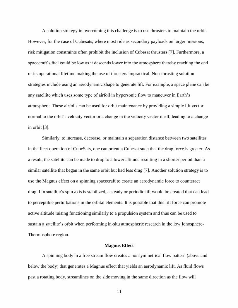
A solution strategy in overcoming this challenge is to use thrusters to maintain the orbit.
However, for the case of Cubesats, where most ride as secondary payloads on larger missions,
risk mitigation constraints often prohibit the inclusion of Cubesat thrusters [7]. Furthermore, a
spacecraft’s fuel could be low as it descends lower into the atmosphere thereby reaching the end
of its operational lifetime making the use of thrusters impractical. Non-thrusting solution
strategies include using an aerodynamic shape to generate lift. For example, a space plane can be
any satellite which uses some type of airfoil in hypersonic flow to maneuver in Earth’s
atmosphere. These airfoils can be used for orbit maintenance by providing a simple lift vector
normal to the orbit’s velocity vector or a change in the velocity vector itself, leading to a change
in orbit [3].
Similarly, to increase, decrease, or maintain a separation distance between two satellites
in the fleet operation of CubeSats, one can orient a Cubesat such that the drag force is greater. As
a result, the satellite can be made to drop to a lower altitude resulting in a shorter period than a
similar satellite that began in the same orbit but had less drag [7]. Another solution strategy is to
use the Magnus effect on a spinning spacecraft to create an aerodynamic force to counteract
drag. If a satellite’s spin axis is stabilized, a steady or periodic lift would be created that can lead
to perceptible perturbations in the orbital elements. It is possible that this lift force can promote
active altitude raising functioning similarly to a propulsion system and thus can be used to
sustain a satellite’s orbit when performing in-situ atmospheric research in the low Ionosphere-
Thermosphere region.
Magnus Effect
A spinning body in a free stream flow creates a nonsymmetrical flow pattern (above and
below the body) that generates a Magnus effect that yields an aerodynamic lift. As fluid flows
past a rotating body, streamlines on the side moving in the same direction as the flow will

12
converge, indicating a diminished pressure [8]. The streamlines on the opposite side move
against the freestream and as a result, become more widely spaced, indicating an increase in
pressure. This pressure differential causes a lifting force that will displace the body in a direction
normal to the freestream flow as shown in Figure 1-1.
Figure 1-1. Magnus force for flow over a spinning spacecraft
This effect has been the subject of great interest in the history of fluid physics and is
named after Professor Gustav Magnus who established that a lifting force is developed by a
spinning cylinder placed in an air flow [9]. Similarly, Newton observed that a transverse force
acts on a spinning sphere moving through a fluid and Robins observed a similar effect in the
trajectory of cannon balls [8]. A description of the Magnus effect was given by Lord Rayleigh
who predicted that the lift was proportional to the speed of rotation and translation. Some of the
earliest inventions incorporating this effect included the Flettner rotor which was a sailboat
whose sail used a rotating cylinder, which produced a Magnus lift thereby generating a thrust to
push the boat forward.
Motivation
The Magnus force is a function of the radius, air density, body spin rate, and freestream
velocity and therefore as the altitude decays, atmospheric density increases thereby increasing
the magnitude of this force. Active altitude adjustments using the proposed Magnus effect on a
13
spinning spacecraft could serve as an orbital maneuver capability without requiring conventional
thrusters. As a result, this added maneuverability could improve efforts to maintain a low perigee
orbit and aid in performing in-situ atmospheric research in the low Ionosphere-Thermosphere
region. This could be significantly more effective for planets with higher atmospheric densities
including Venus whose atmosphere is mostly made up carbon dioxide.
Equally important, the Magnus effect could be used to perform active, controlled
deorbiting to improve predictions of the impact location. This could benefit satellites near End-
of-Life (EOL), or for systems that fail to fully demise during the reentry process. For example,
between 10% and 40% of a spacecraft’s mass is destroyed by the extreme reentry conditions
where the remainder poses a threat to ground as well as air traffic [10]. Notably, several events
have previously occurred that illustrate the importance of predicting the reentry location a priori
including the uncontrolled reentry of Russia’s Phobos-Grunt, which resulted in the closing of the
European airspace for two hours [10]. Most importantly, a study conducted by the FAA
following the disintegration of space shuttle Columbia in 2003, found that the probability of an
impact between Columbia debris and a general aviation aircraft was one in a hundred [10].
According to the Aerospace Corporation, there are about 100 large man-made objects that
reenter the earth’s atmosphere randomly each year [10]. In addition, there are more than 20,000
pieces of debris larger than a softball orbiting the earth that travel at speeds up to 17,500 mph,
which is fast enough for a relatively small piece of orbital debris to damage a satellite or
spacecraft [11]. Current predictions of the time and location of uncontrolled reentries may have
errors of several thousand kilometers and are available only minutes before reentry [10]. As a
result, NASA has guidelines on how to deal with potential collision threats including if the
probability of collision is greater than 1 in 100,000, a maneuver will be conducted if it will not

14
result in a significant impact to mission objectives [11]. Thus, there exists a need for improving
knowledge of the reentry impact location to mitigate the risk of collision between space debris
and other ground stations, which could possibly be achieved using the Magnus effect.
Consequently, Chapter 2 of this thesis, will examine the feasibility of the Magnus effect
in sustaining a spacecraft’s orbit where continuum and free-molecular theory is used to formulate
the appropriate force as a function of the altitude. The magnitude of this force on the orbital
decay will be examined by varying the altitude of apogee, satellite body spin rate, and satellite
mass for a spherical spacecraft having an initial mass of 25 kg and a radius of 1 m. A literature
review is also performed to provide an understanding of the aerodynamic forces acting on a
rotating sphere in a continuum and free molecular regime. Lastly, a way to generate the required
body spin rate will be briefly reviewed. Chapter 3 will then address some of the challenges in
implementing the Magnus phenomenon for a spacecraft.
Challenges
A spinning spacecraft can be described as a bearingless or free rotor and consequently
there is a need in designing a mechanism to protect the rotor from external loads [12]. As a
result, a system to shield the Magnus rotor from the forces experienced during the launch
environment or during transport in space is required. This is in contrast to fixed rotors which are
usually suspended through a set of cylindrical hinges or bearings that allows it to rotate freely
about an axis fixed in space [12]. A way to protect the rotor prior to release could be achieved by
using spring-loaded contacts to secure the rotor from external loads as shown in the left of Figure
1-2.
To clarify the concept, the Magnus rotor would be covered with a vacuum-compatible
thermal grease, which would then be spring-loaded at various contact points. The springs would
be supported by the spacecraft’s external housing. When the system is ready to operate, the rotor

15
would passively release itself by spinning hence creating a pressure field of sufficient intensity to
overcome the preload force.
Figure 1-2. Concept of a passive release mechanism a) Spring-loaded with grease b) Non-
conformal contact of a spinning cylinder against a plane
Therefore, in order to provide insight into designing a passive release system for a
Magnus spacecraft, Chapter 3 of this thesis will investigate the tribology of a rotating cylinder
against a plane as shown in the right of Figure 1-2. The problem of a Magnus rotor spinning
against a spring-loaded contact point can be simply represented by a non-conformal contact.
Non-conformal contacts are contacting surfaces that do not conform well to each other as seen in
ball bearings and the resulting load is carried over a small contact area [13]. CFD simulations
will be conducted to examine the pressure field in the grease as a function of the rotational speed
of the rotor and film thickness. An empirical equation for the pressure will be developed and
subsequently compared with an analytical solution to compare the difference in using the
parabolic film against the true circular film thickness approximation. A literature survey will be
provided to examine references that have used the parabolic film approximation in deriving the
a) b)

16
pressure field in bearing applications. Finally, Chapter 4 of this thesis will summarize the
conclusions of the Magnus feasibility study and provide recommendations for future research.

17
CHAPTER 2
MAGNUS EFFECT ON A SPINNING SATELLITE IN LOW EARTH ORBIT
This chapter investigates the feasibility of using the Magnus effect in sustaining a
spacecraft’s orbit at a perigee of 80 km. Since the Magnus force is a function of the freestream
density, this research is restricted to a low perigee altitude. A literature review is first conducted
to examine how various environmental perturbations can affect a satellite’s orbit evolution.
Acquiring an understanding of these perturbations will provide insight on how the Magnus force
might affect a satellite’s orbit evolution. Subsequently, another literature review is done to
develop an expression for the Magnus force in the continuum and free-molecular regime for
implementation in the Systems Tool Kit (STK) software. To clarify, in LEO the interaction of
the molecules can be described as free-molecular or a continuum depending on the mean free
path of the fluid, which is the average distance particles or molecules travel between collisions
[14]. If the mean free path is small in comparison with the dimensions of the body then the fluid
can be considered a continuum. With this assumption, the fluid’s properties (i.e. density,
temperature, and velocity) has a definite value at each point in space. However, many modern
engineering applications, including those for spaceflight, occur at high altitudes where the mean
free path is not negligible when compared with the dimensions of the body and therefore the
effects of the discrete character of the fluid must be taken into account when defining its
properties [15]. At these two different regimes, the governing physics and interaction of the
molecules are different. For example, in a continuum flow regime, the Magnus force on a
rotating body is more prominent due to the increase in the surrounding gas density. However, in
a rarefied gas flow in the absence of intermolecular collisions, the magnitude of the Magnus
force is reduced and the direction is opposite to that in a continuum flow at small Reynolds
numbers [16].
18
A review on orbit perturbations and methods of solution are described in this chapter and
the methodology in modeling the Magnus force will be explained. Simulation results will be
presented where the effects of changing the altitude of apogee, satellite body spin rate, and
satellite mass are investigated for a spherical spacecraft with a radius of 1 m.
Literature Review on the Magnus Effect
In order to accurately model the Magnus force a literature review was conducted to learn
how a lift perturbation affect a satellite’s orbital evolution and to learn more about the gas-
surface interaction between the incident gas molecules and the satellite’s surface. After, a
subsequent literature review was done to determine how the magnitude of the Magnus force
changed in the free molecular regime, to the transitional flow regime, and finally to a continuum
regime.
The Effect of Lift on a Satellite’s Orbit
To begin with, Cook [17] explains that for satellites that remain stabilized for long
intervals of time, one must reexamine the effect of the aerodynamic lift. Cook investigates a
constant lift to drag ratio acting on a flat plate satellite. Regarding the gas-surface interaction,
Cook considers the simplest case of hyperthermal free-molecule flow where the thermal
accommodation coefficient ατ = 1, for which the random thermal motion of the molecules is
assumed negligible compared with the satellite’s speed. To clarify, a thermal accommodation
coefficient of one represents a diffusive reflection where the molecules are reflected with a
random distribution of speed and direction [18]. For example, below 200 km, atomic oxygen, a
principal constituent of the thermosphere, is absorbed on the surface, causing the incident
molecules to be diffusely re-emitted [19]. Above 200 km, the accommodation coefficient
becomes lower and approaches specular reflection. Specular reflection, or when the thermal

19
accommodation coefficient is zero, is when the angle of reflection equals the angle of incidence
[17].
With complete accommodation or with a thermal accommodation coefficient value of 1,
the lift to drag ratio will be on the order of 0.05. With no accommodation, Cooke describes that
the lift to drag ratio can be high as 2/3 and therefore the importance of lift depends on the nature
of the momentum exchange at the satellites surface. Furthermore, Cook goes on to explain that
since lift acts perpendicular to the satellite’s velocity vector, it can have no effect on the semi-
major axis of the orbit. Consequently, one should only be concerned with variations of the
eccentricity vector. In order for the orbital inclination to change, a component of force normal to
the orbital plane is required [20]. For the constant lift coefficient case, Cook finds that the
eccentricity remains constant and the only effect of lift is to rotate the major axis. Therefore, this
thesis will also assume a hyperthermal free molecular flow regime due to the low perigee
altitudes examined. Assuming a primarily diffusive reflection as the satellite descends into the
atmosphere will result in a conservative approximation for the Magnus force. Also, since the
Magnus force acts perpendicular to the velocity, it is seen that it will not affect the semi-major
axis of the orbit.
Ashenberg in [21] presents solutions for a satellite with non-constant aerodynamic
coefficients using the Gaussian form of the Lagrange Planetary Equations. Ashenberg describes
that if a satellite has dominant flat surfaces, rotates at certain slow rates, or has a large area to
mass ratio, the lift forces do not average out to zero. In addition, a varying aerodynamic lift can
occur for solar sails where the direction of the sail relative to the sun can change thereby
changing the direction of the force exerted by the sunlight. The perturbations are projected in the
normal direction given by hxV toward the inside of the orbit, where h is the orbital angular

20
momentum and V is the satellite’s velocity and calculations are done assuming free molecular,
hyperthermal flow. Ashenberg describes how the lift acting in the orbital plane perturbs the
eccentricity vector, while an orthogonal (out-of-plane) force perturbs the orientation of the
orbital plane. Significantly, Ashenberg states that since the lifting force does not change the
energy, the semi-major axis is perturbed by drag alone. The general conclusion is that time-
varying aerodynamic coefficients may cause various forms of secular orbital motion. Similarly,
this thesis will consider the Magnus force as only acting in the orbital plane and thus a new
coordinate frame in the hxV direction will be defined for the STK simulations.
Moore [22] also describes how satellites in stabilized attitudes may be subjected to steady
or periodic lift giving rise to perceptible perturbations in the orbital elements. He uses the
LaGrange equations of motion to study the effects of lift and drag on the orbital elements and
states that the precise determination of lift effects require either in-situ examination of the gas-
surface interaction or detailed analysis of orbital perturbations and spin rate data. He describes
the hyperthermal free molecular flow as being where the mean free path of the molecules is very
large compared with the dimensions of the satellite and where the molecules have no random
thermal motion. Reviewing the work of Cook [17], Ashenberg [21], and Moore [22], it is seen
that the Magnus force will affect a satellite’s eccentricity vector and the hyperthermal free
molecular flow assumption will be appropriate for the low perigees investigated for this
feasibility study. The work of these authors were all focused on applying the concept of lift to
flat plate satellites in the free molecular regime that were attitude stabilized. However, the
concepts explored in these papers will provide insight into understanding how the Magnus
perturbation will affect a satellite’s orbit where the satellite will be assumed to be spin stabilized
or in pure rotation. A more detailed literature review is now done to examine how the Magnus

21
force on a spinning sphere changes from the free molecular to the continuum regime. As a result
of the increase in density as one descends lower into the atmosphere, one must consider
parameters including the Reynolds number and Knudsen number.
Aerodynamic Lift on a Spinning Sphere
The Knudsen number (Kn) is a widely recognized parameter that determines whether a
fluid medium is a continuum (Kn <<1) or free molecular (Kn >>10), which is the ratio of the
mean free path and the macroscopic length scale of the physical system. In other words, the local
Knudsen number is a measure of the degree of rarefaction of a gas [23]. Thus, at altitudes higher
than 100 km, free molecular conditions will prevail. Subsequently, the flow will move into
transition flow as the Knudsen number decreases in the range of 0.1 < Kn < 10 and then into slip
flow where the no-slip boundary condition starts to break down or when 0.001< Kn < 0.1.
Finally, when the Knudsen number falls below 0.001, a continuum flow regime can be assumed.
Wang in [24] determines the aerodynamic forces for free molecular flow over a rotating
sphere. Most importantly, he describe that in the free molecular regime, the Magnus force exerts
a negative lift on the sphere. Literature was now explored that described the Magnus force in the
transitional and continuum regime. For example, Volkov [16] numerically investigates the 3D
rarefied gas flow past a spinning sphere in the transitional and near continuum flow regimes.
Volkov describes that in a rarefied gas flow in the absence of intermolecular collisions, the
direction of the Magnus force is opposite to that in a continuum flow at small Reynolds numbers.
He describes that the Magnus lift coefficient is a sum of the normal and tangential stresses acting
at the surface of the sphere as shown in Eq. (1-1),
𝐶𝐿 = 𝐶𝐿(𝑛) + 𝐶𝐿(𝜏) (1-1)

22
where 𝐶𝐿(𝑛) and 𝐶𝐿(𝜏) is the fraction of 𝐶𝐿 created from distributions of the normal and
tangential stresses. In the transitional flow regime, the contribution from the normal stresses is
always positive or 𝐶𝐿(𝑛) > 0. However, with a decrease in Kn as one approaches the transitional
regime, the contribution of the tangential stresses is much more complex than in the free
molecular regime and 𝐶𝐿(𝜏) decreases in absolute value. Therefore, the direction of the Magnus
force in the transitional regime is determined by the balance between the normal and tangential
stresses on the sphere’s surface. As a result, the direction of the force or the sum of Eq. (1-1)
changes sign at a certain Knudsen number. Volkov describes that with a decrease in the Knudsen
number, the Magnus lift coefficient should first increase from -4/3 to the maximum value of 2 in
the continuum flow regime at small Reynolds numbers and then decrease to the limiting value
corresponding to large Reynolds numbers.
Equally important, the Magnus effect in the continuum regime was then examined where
Rubinow and Keller [25] derive an expression for the Magnus force in the continuum limit using
the Navier-Stokes equations assuming small Reynolds number. It is shown that at small
Reynolds numbers, the rotation of the sphere does not affect its drag force coefficient. In
addition, Rubinow and Keller states that in the continuum regime at small Reynolds numbers the
aerodynamic torque exerted on the spinning sphere is independent of the translational velocity of
the sphere relative to the fluid. An equation for calculating the aerodynamic torque for a spinning
sphere at a low Reynolds number is given.
Thus, reviewing the work of Wang and Volkov allows one to develop an appropriate
expression for the Magnus force as a satellite descends from the high altitudes in the free
molecular regime to low altitudes in the continuum regime. The results from Rubinow and Keller
allow one to change the rotational speed of the satellite while keeping the drag coefficient the

23
same. Significantly, the formula for the aerodynamic torque from Rubinow and Keller will be
used in determining a possible method in generating the required body spin rate for the Magnus
effect.
Finally, a literature review was conducted to examine the motivation of maintaining a
low perigee orbit in LEO. Hall [26] investigates multiple orbital schemes and maneuvers using
electric propulsion along the satellite’s velocity vector to determine the feasibility of
counteracting the drag force at a perigee of 100 km. He describes how elliptic orbits utilizing a
very low perigee can facilitate access to the surface and atmosphere at sub-ionosphere altitudes
while counteracting drag using continuous electric propulsion. Low perigee orbits has been
studies for interplanetary scientific missions and has a significant potential for remote sensing.
Likewise, the current efforts in this Thesis is to counteract drag at a low perigee without using
conventional thrusters or by using a continuous Magnus effect.
Orbit Perturbations
To understand the governing equations of orbital decay of satellites in LEO the equations
of motion for the two-body problem must first be examined. The physical motions of each planet
was first addressed by Kepler where he summarized that 1) the orbit of each planet is an ellipse
with the sun at a focus 2) the line joining the planet to the sun sweeps out equal areas in equal
times and 3) the square of the period of a planet is proportional to the cube of its mean distance
from the sun [6]. Newton then mathematically explained why planets and satellite followed an
elliptical orbit by combining his Law of Universal Gravitation and his Second Law of Motion
resulting in Eq.(2-1). This equation describes the satellite’s position vector relative a central
body (e.g. earth) and assumes that: gravity is the only force acting on the system, the central
body is spherically symmetric, the central body’s mass is much greater than the satellite’s mass,
and the central body and the satellite are the only two bodies in the system [27]. To clarify, r is

24
the position of the satellite relative to Earth’s center and this differential equation is a second
order, nonlinear, differential equation.
�̈� + (𝜇𝑟−3)𝐫 = 0 (2-1)
A solution to the two-body equation of motion for a satellite orbiting earth is the polar
equation of a conic section [27]. In order to solve Eq. (2-1) six constants of integration or initial
conditions are required and thus one can define the orbit with six classical orbital elements with
one quantity varying with time as shown in Figure 2-1.
Figure 2-1. Keplerian orbital elements of a satellite in an elliptic orbit.
A brief summary of the classical orbit elements as described in [27] includes:
Semi-Major Axis (a): defines the size of the orbit
Eccentricity (e): defines the shape of the orbit
Inclination (i): the angle between the angular momentum vector ℎ⃑ and unit vector Z⃑
which points in the direction of the North Pole.
Right Ascension of the Ascending Node (RAAN Ω): The angle from the vernal equinox
to the ascending node. The ascending node is the point where the satellite passes

25
through the equatorial plane moving from south to north.
Argument of Perigee(ω): The angle from the ascending node to the eccentricity vector
measured in the direction of the satellite’s motion. The eccentricity vector points from
the center of the earth to perigee with a magnitude equal to the eccentricity of the orbit.
Mean anomaly (M): The fraction of an orbit period which has elapsed since perigee
expressed as an angle. The mean anomaly equals the true anomaly for a circular orbit.
Equations of Motion with Perturbations
A satellite will always remain in orbit and consequently its orbital elements will remain
constant if gravitational forces are the only force acting on it. However, when other perturbations
are present, the two-body problem becomes Eq. (2-2) implying that orbital lifetime becomes
shorter or longer depending on 𝐚𝐏, the resultant vector of all the perturbing accelerations.
�̈� +𝜇
𝑟3𝐫 = 𝐚𝐏 (2-2)
Some of these perturbing acceleration terms include atmospheric drag, solar radiation
pressure, Earth’s oblateness, and other (n-body effect) [6]. In the solar system, the sum of the
perturbing accelerations for all satellite orbits is at least 10 times smaller than the central force or
two-body accelerations or aP << 𝜇
𝑟3 [28]. The non-homogenous equation in Eq. (2-2) implies that
the semi-major axis a, orbit angular momentum h, and eccentricity e are not constants but satisfy
[17],
�̇� =2a2
μ�̇� ∙ 𝐟
(2-3)
ℎ̇ = 𝐫 x 𝐟 (2-4)
�̇� =1
𝜇{𝐡 x 𝐟 + (𝐫 x 𝐟) 𝐱 �̇� }
(2-5)

26
Methods of Solution
A deviation from Keplerian motion includes secular and periodic perturbations. Secular
perturbations are those which the effects build up over time while periodic or cyclic
perturbations are such that the effects cancel after one cycle or orbit [28]. Furthermore, secular
changes in a particular element vary linearly over time or proportionally to some power of time.
The largest perturbation is due to gravitation, followed by drag, third body perturbations, and
solar radiation pressure effects. Third body effects are perturbations caused by the attraction of
the sun, moon, and other planets and satellites. In addition, solar radiation pressure is when
photons impact a satellite’s surface and are reflected or absorbed.
Techniques to solve the two-body problem with perturbations encompass numerical,
analytical, and semi-analytical methods. In using these methods, the primary difference is
whether one uses the satellite’s position and velocity state vectors or the orbital elements as the
elements of state. Typically analytical methods are faster but the expressions are truncated to
allow simpler expressions. As a result, the computational speed increases but accuracy decreases.
Numerical approaches consists of numerically integrating the perturbing accelerations. The
numerical approach can also be applied to the Variation of Parameter (VOP) equations in which
case a set of orbital elements are numerically integrated [28].
Furthermore, the three main methods to solving the equations of motion with
perturbations are special perturbation (numerical), general perturbation (analytical), and semi-
analytic. Special perturbation techniques include Cowell’s method and Encke’s method, which
uses numerical integration of the equations of motion including all perturbing accelerations [28].
This approach uses the position and velocity vectors of the satellite. However, the analytical
approach uses the orbital elements for integration while semi-analytic methods uses a
combination of numerical and analytical techniques.

27
Most analytical and few numerical approaches use the VOP form of the equations since
the orbital elements in the two-body equation are changing. Lagrange and Gauss both developed
VOP methods to analyze perturbations. Lagrange’s technique applies to conservative
accelerations while Gauss’s approach can also be implemented for non-conservative
accelerations. Conservative accelerations are explicitly a function of position only and there is no
net transfer of energy taking place and therefore the mean semimajor axis of the orbit is constant.
However, non-conservative accelerations are explicitly a function of both position and velocity
including atmospheric drag, outgassing, and tidal friction effect where energy transfer occurs
thereby changing the semimajor axis. [28]. Drag is a non-conservative force and will
continuously reduce the energy of the orbit decreasing the semi-major axis and period. The orbit
will become more circular each revolution and will then rapidly spiral inwards due to the dense
atmosphere. Using the VOP technique, one can examine the effects of perturbation on specific
orbital elements. In the Gaussian VOP, the rates of change of the elements are explicitly
expressed in terms of the disturbing forces. Since a low perigee of ~80 km will be examined, the
dominating perturbing force will be from drag and the Magnus effect allowing one to ignore
other perturbations. Significantly, one can see that the Magnus force will change as a function of
time since it primarily depends on the atmospheric density classifying it as a secular, non-
conservative force.
Modeling the Magnus Effect
Numerical propagation of a satellite’s trajectory using the Magnus effect would consist of
many interacting components including: a numerical propagator that solves the equation of
motion and a force model that evaluates the effect of the Magnus force on the satellite. Since the
current study is examining the feasibility of the Magnus force, it was decided to model its effect
as a super-efficient thruster for simplicity. The Systems Tool Kit (STK) allows the user to

28
incorporate customer specific modeling into the computations by creating a plugin, which
provides a method for customizing STK. The equations of motion are integrated using the
Runge-Kutta-Fehlberg method of 7th order with 8th order error control [26]. However, before
beginning to perform the simulations, a test case was first performed to validate that STK was
being used correctly. The simulation validation case was taken from Hall [26], whom used STK
to examine the final altitude for a constant initial perigee altitude of 100 km with an increasing
apogee altitude between 2,622 km to 18,622 km. A 150 mN of continuous thrust was applied
along the velocity vector from perigee to apogee. The satellite was then allowed to coast back to
perigee without the use of any thruster and this sequence was repeated 100 times. After the end
of the sequence, the final apogee and perigee altitudes are recorded at the termination of the
simulation as shown in Figure 2-2. There is good agreement between the STK simulation and by
Hall giving confidence that the user was correctly using STK.
Super-Efficient Thruster Model
The Magnus force perturbation can be expressed as Eq. (2-6),
𝐅𝐦 =1
2𝐶𝐿𝜋𝑟3𝜌∞𝛚x𝐕
(2-6) where r is the radius of the sphere, CL is the lift coefficient, ω is the body angular
velocity or body spin rate assumed to act normal to the orbital plane, V is the freestream
velocity, and ρ is the freestream density.
For this feasibility study of the Magnus effect, it was determined that it would be
sufficient to model the Magnus force in Eq. (2-6) as a thruster. Moreover, STK has an engine
plugin feature where users can add modeling capabilities that are not available on the graphical
user interface. A plugin is a user-supplied software component called by the application at
certain pre-defined event times within the STK computation cycle [29]. An engine plugin script
was written using Visual Basic Scripting (VBS) that pulls in the instantaneous density, altitude,

29
and magnitude of the velocity during each time step in STK to evaluate the Magnus force in Eq.
(2-6). Theoretically, one does not have the capability to incorporate a high body spin rate on the
actual satellite in STK and thus the Magnus force is not physically modeled. As a result, an
initial body spin rate magnitude of 5000 RPM and a constant radius of 1 m is assumed in order to
evaluate Eq. (2-6) for the engine plugin. However, the magnitude of the thruster in the
simulations closely matches the magnitude for the theoretical Magnus force.
Figure 2-2. There is good agreement between the STK simulation (top) and Hall’s results
(bottom)

30
In modeling the Magnus effect as a thruster, a fuel mass of 5 kg was used since STK
requires this parameter for its thruster implementation. As a result, it was exceedingly important
to make sure that a negligible amount of fuel was lost for each simulation to closely simulate the
Magnus effect. For instance, if a large amount of fuel was lost, then the area to mass ratio of the
satellite would change during the simulation thereby affecting its orbital lifetime. Consequently,
it would not be a valid comparison in relating the decay of the satellite with the Magnus force.
Therefore, to most closely model the Magnus force, an exceedingly high specific impulse of
2x10¹² s was used for the engine to ensure that the mass of fuel consumed for each simulation
was negligible. For example, with a high specific impulse of 2x10¹² s the mass of fuel consumed
for each simulation was negligible, (~3x10-13 kg), allowing one to approximately model the
Magnus effect.
Pulling in the instantaneous altitude during each time step in STK allows one to evaluate
the lift coefficient in Eq. (2-6). The lift coefficient for the Magnus force, as described by [16],
[8], and [24], is negative in the free molecular regime and depends on ατ, the thermal
accommodation coefficient as shown below in Eq. (2-7). Thus, with a diffusive reflection
assumption, (ατ = 1), one can see that the lift coefficient in Eq. (2-7) will be -4/3 in the free
molecular regime.
𝐶𝐿 =−4
3 ατ
(2-7) As stated previously, Volkov [16] describes that with a decrease in the Knudsen number,
the value of Cl should first increase from -4/3 to the maximum value of 2 corresponding to the
continuum flow regime at small Reynolds number. As a conservative approach, the reflection is
assumed to be purely diffusive with complete accommodation (ατ = 1) [30]. With a purely

31
diffusive assumption as opposed to a specular reflection, the lift is small compared to drag and
results in a conservative approximation for the Magnus force.
To create a realistic model and a smooth transition between the changing lift coefficients
as the satellite’s trajectory descended from a free molecular regime to continuum regime, the
hyperbolic tangent function was used. However, in order to decide what approximate altitudes
the Magnus lift would change from negative to positive, the Knudsen number was first
calculated using the expression below in Eq. (2-8) taken from [31],
Kn = √𝜋
2𝑅𝑇
𝜇
𝜌𝐷
(2-8)
where, 𝜇 is the dynamic viscosity, R is the specific gas constant, D is the diameter of the
sphere, and T is the temperature at a given altitude. Examining the results from Eq. (2-8) in Table
2-1, one can approximate that the continuum regime starts at altitudes less than 80 km or where
Kn < ~ 0.001 assuming a satellite radius of 1 m. A calculation of the Reynolds number can be
found in Appendix A.
Table 2-1. Knudsen number at varying altitudes
Altitude, km Kn
100 0.0619
86 0.0049
80 0.0019
70 0.0004
66 0.0005
Thrust Axes
To ensure that the thrust was always perpendicular to the satellite’s velocity vector, a new
reference frame was defined for the Magnus force based on the cross product of the velocity of
the satellite,𝐕, and its orbit angular momentum 𝐡. It is assumed that the satellite is in pure
rotation where the body’s angular momentum vector is parallel to the orbit angular momentum

32
vector. Thus, with this assumption the spin axis is assumed to lie perpendicular to the orbital
plane resulting in the lift vector acting in the orbital plane. With the spin axis perpendicular to
the orbital plane, this thesis will refer to the body angular velocity vector as the body spin rate.
The Magnus force direction was set using an aligned and constrained axes feature in STK
as described in [29], where the aligned vector was set to Vxh. Please see Appendix B, which
illustrates the STK graphical user interface for creating the coordinate frame. In using the orbit
angular momentum in defining the direction of the thrust, a calculation was done to establish that
the orbit angular momentum was significantly greater than the satellite’s body angular
momentum. Please refer to Appendix C which demonstrates that the orbit angular momentum is
significantly greater than the satellite’s body angular momentum for a body spin rate magnitude
of 5000 RPM.
Hyperbolic Tangent Function
After calculating the altitude where continuity conditions prevailed, the hyperbolic
tangent function was used to create a smooth transition from the negative lift coefficient in the
free-molecular regime to the positive lift coefficient in the continuum regime as described by the
literature. This function has been used before to model a smooth transition between two
functions [32]. The developed function can be seen in Eq. (2-9) and Figure 2-3, where x is the
altitude of the satellite.
Thus, the super-efficient Magnus engine plugin is implemented using Eq. (2-6), which
evaluates the Magnus lift coefficient based on the instantaneous altitude of the satellite in STK as
seen in Eq. (2-9). Pleases refer to Appendix D for the Matlab code for the hyperbolic tangent
function fit and Appendix E for the VBS code for implementing the super-efficient thruster.
𝐶𝐿 =1
3−
5
3∗ tanh(2 ∙ 𝑥 − 164)
(2-9)

33
Figure 2-3. Hyperbolic tangent function creates a transition between positive and negative
Magnus Lift.
STK Astrogator Settings
Drag is incorporated into the simulations and is based upon the Jacchia-Roberts
Atmospheric density model. The coordinate system used in the simulations is the VNC
(Velocity-Normal-Conormal) reference frame. In this frame, the X-axis is along the velocity
vector V, the Y-axis is along the orbit normal or Y =rxV, and the z-axis completes the
orthogonal triad. The orbit epoch time is set to October 4th, 2012 12:00. The Magnus thruster is
modeled as a finite maneuver which is effectively a propagate segment with thrust. It uses the
defined propagator to propagate the state accounting for the acceleration due to thrust. Each
point calculated during the numerical simulation is added to the satellite’s ephemeris until a
stopping condition is met [33]. In STK’s Astrogator, two separate finite maneuvers are
implemented with the custom engine plugin to account for the change in the Magnus lift
coefficient as the satellite descends from a free molecular regime to a continuum regime. Initially
the satellite is not in the continuum regime (≥84 km), and thereby the first maneuver puts the
Magnus direction as equal to hxV to account for the negative Magnus force. Under 84 km,
another finite maneuver is done to implement the thrust acting in the Vxh direction. As
previously stated, the mass is set to 20 kg with 5 kg of fuel defined with a cross sectional area of

34
3.14 m2 assuming a spherical geometry with a radius of 1 m. As a note, the mass of fuel needs to
be defined in order for STK to perform the simulations even if the fuel consumption is very low.
The drag coefficient is set to a value of 2 as described in [24] that is based on the hyperthermal
free molecular assumption, where one assumes the reflection is purely diffusive with complete
accommodation (ατ = 1). Also, for all simulations, a decay altitude of 65 km was used.
Correct Implementation of Formula
Before performing the required simulations, a test case was performed to ensure that the
custom engine plugin was working correctly. The Magnus thruster plugin was programmed to
pull in the atmospheric density, altitude, and the velocity magnitude of the satellite from STK
during each time step. With an assumed body spin rate magnitude of 5000 RPM and radius of 1
m, and using the density and magnitude of the velocity output from STK, one can plot the
expected theoretical thrust given by Eq. (2-6) against the magnitude of the thrust output
simulated in STK. Looking at Figure 2-4, one can see that the good agreement between the STK
simulation and the theoretical calculation ensures that the user-defined thruster is accurately
pulling in the density and velocity as a function of time.
In addition, as seen in Figure 2-4, the lift coefficient is initially negative since the satellite
is in the free molecular regime. However, as the altitude decreases (< 84km) one can start to see
a rapid increase in thrust and see that the thrust is no longer negative This is expected since the
satellite is now in the continuum regime. One can see that the magnitude of the thrust acting on
the satellite starts to oscillate as shown in Figure 2-4 as a result of the interaction between the
drag, gravitational force, and Magnus effect.
To clarify, as the satellite descents lower in the atmosphere, the density increases
producing a larger Magnus thruster increasing the altitude of the satellite. However, as the

35
altitude increases, the density decreases reducing the effect of the Magnus thruster causing the
thrust to oscillate.
Figure 2-4. Verifying Magnus Thruster implementation is correct
Body Spin Rate Required to Avoid Losing Height
After verifying that the Super-efficient thruster was being implemented correctly, an
analysis based on [3] was then performed to examine the magnitude of the body spin rate
required for a satellite not to lose altitude using the equation for the Magnus lift and drag as seen
in Eq. (2-10) and (2-11). This rough analysis gives one insight on the magnitude of the body
spin rate, radius, and altitude that should be examined for this study. For a conservative
approximation, the Magnus lift for a spinning sphere in free molecular flow was used for Eq. (2-
10), which can be found in [24] and [16],
𝐿 =2
3𝜋𝑟3𝜌𝜔𝑉
(2-10)

36
𝐷 =1
2𝜌𝐶𝑑𝐴𝑉2
(2-11)
where 𝑟 is the radius of the sphere, 𝜌 is the density at a given altitude, 𝜔 is the body spin
rate magnitude of the satellite in rad/s, V is the magnitude of the satellite’s orbital velocity, 𝐶𝑑 is
the drag coefficient, and A is the reference area.
Given a mass of 25 kg and a radius of 1 m, the body spin rate magnitude of the satellite is
used as the independent variable in this example. Assuming the satellite travels through the
atmosphere with a flight path angle of 0°, the required body spin rate magnitude as a function of
different radii at different altitudes can be found using the free body diagram of Figure 2-5,
where the only assumed forces acting on the satellite are lift, drag, and weight. A flight path
angle of 0° would give the maximum body spin rate required. Summing the forces in the x and y
direction results in Eq. (2-12) which is the required body angular velocity of the sphere to avoid
losing altitude,
𝜔 =3𝑚𝑔 𝑐𝑜𝑠 ∅
2𝜋𝑟3𝜌𝑉
(2-12)
where, m is the mass, g is the gravitational acceleration, ∅ is the flight path angle, r is the
radius, and V is the orbital velocity.
Figure 2-5. Simplified Magnus force analysis in a continuum regime.

37
Figure 2-6. Satellite body spin rate magnitude and radius required to avoid losing height.
Using the 1976 Standard Atmosphere Model, a velocity magnitude of 7.5 km/s, and a
constant mass of 25 kg, the required body spin rate magnitude to avoid losing altitude was
calculated by summing the forces in the x and y direction for different altitudes and is plotted in
Figure 2-6.
As the magnitude of the body spin rate increases, the radius required to produce the
required lift to avoid losing altitude decreases. Also, as the altitude increases, the resulting low
density requires an exceedingly large radius to generate the required lift. Examining this
analysis, might encourage one to believe that the Magnus effect is impractical due to the high
required spin rates. However, this study will demonstrate that in a low perigee altitude of 80 km,
a body spin rate magnitude of 5000 RPM, and a 1 m radius sphere is sufficient for delaying the
reentry period assuming a decay altitude of 65 km.
Simulations Using STK
To investigate the feasibility of using the Magnus effect on a spinning spacecraft to
prolong its trajectory in a regime of considerable density, the altitude of apogee was first varied
while keeping the altitude of perigee at 80 km. Subsequently, the next step involved changing the

38
magnitude of the Magnus thruster by theoretically increasing the rotational speed of the satellite.
Finally, a simulation was conducted at different masses to examine the effect on the feasibility of
the Magnus effect.
Maintaining Altitude of Perigee
Performing initial simulations in STK demonstrated that the Magnus effect was only
effective at altitudes around 80 km due to the increase in atmospheric density. Thus, the first
analysis examined the effect of holding the altitude of perigee constant at 80 km while increasing
the altitude of apogee or eccentricity of the orbit as shown in Table 2-2.
Table 2-2. List of orbital elements for an altitude of perigee = 80 km
Apogee Altitude e i Ω (deg) ω (deg) M (deg)
145.18 0.005 40 0 0 180
177.88 0.008 40 0 0 180
210.74 0.010 40 0 0 180
411.46 0.025 40 0 0 180
760.08 0.050 40 0 0 180
1127.54 0.075 40 0 0 180
1515.42 0.100 40 0 0 180
2359.62 0.150 40 0 0 180
3309.34 0.200 40 0 0 180
4385.70 0.250 40 0 0 180
Examining the results in Figure 2-7, one can see that using 65 km as the decay altitude,
the Magnus effect approximately doubles the amount of time in orbit assuming a body spin rate
magnitude of 5000 RPM.
This extension of time on orbit could possibly be used by a spacecraft to maneuver itself
to an area that will reduce the impact of collisions with the airspace. Likewise, the extension of
time on orbit could be used to maintain a low perigee orbit and aid in performing in-situ
atmospheric research in the low Ionosphere-Thermosphere region. Significantly, this could be
more effective for planets with higher atmospheric densities.

39
Figure 2-7. Amount of time on orbit, with and without Magnus Thruster at 80 km Perigee.
Different RPM
Next, the effect of changing the magnitude of the body spin rate in Eq. (2-6) was
performed to see the effect on the time in orbit. The first set of orbital parameters in Table 2-2
(apogee=145.18 km, e=0.005) was chosen as the set to be analyzed. Examining Figure 2-8,
without the Magnus thruster, the time in orbit is around 20 min. However, with the Magnus
Thruster enabled with a body spin rate magnitude of 5000 RPM, the time in orbit until decay is
extended to 60 min. Furthermore, as the body spin rate magnitude is increased to 10,000 RPM no
decay is seen in the orbit within the allotted 20,000 min simulation time and the satellite is seen
to oscillate at an altitude of 66 km.
The behavior of Figure 2-8 is expected as the RPM is increased if one reexamines Figure
2-6, (which is replotted in the right of Figure 2-8 for clarity). For a satellite with a radius of 1 m,
Figure 2-8 illustrates that a body spin rate of at least 7000 RPM or above is required to not lose
height for an altitude of 80 km. Thereby, one can see that the body spin rate of 10,000 RPM-
15000 RPM is over the required minimum of 7000 RPM and thus the satellite’s altitude
oscillates and the STK simulation time is over the time limit threshold of 20,000 min.

40
Figure 2-8. Examining the effect of the body spin rate a) Time in orbit for different body spin
rates b) Radius required not to lose altitude
Different Mass
The last parameter that was changed was the total mass of the spacecraft. Examining
Figure 2-9, for a body spin rate of 5000 RPM, the satellite with 10 kg mass oscillates at an
altitude of 67 km and the lifetime is over 20,000 min. However, the 25 kg satellite’s lifetime is
~56 min and the 50 kg satellite is ~43 min. From a design perspective, in order to use the
Magnus force effectively, one should reduce the mass and increase the radius.
a)
b)

41
Figure 2-9. Time in orbit for different masses.
Generating Body Spin Rate
A way to generate the required body spin rate for a Magnus spacecraft is now briefly
reviewed. As stated in the literature review, Rubinow and Keller states that in the continuum
regime at small Reynolds numbers, the aerodynamic torque exerted on the spinning sphere is
independent of the translational velocity of the sphere relative to the fluid. In addition, Rubinow
and Keller presents a relationship for the torque on the sphere as shown in Eq. (2-13).
𝑇 = 8𝜋𝜇𝑟3𝜔 (2-13)
Assuming a mass of 25 kg, a body spin rate of 5000 RPM, a radius of 1 m, the required
torque to spin can be found as shown in Table 2-3. As the altitude decreases, the Reynolds
number will increase and thereby there is some uncertainty in using the assumption of low
Reynolds number as the altitude goes from 86 km down to 65 km. However, the motivation is to
show a possible way to counteract the aerodynamic torque using commercial off-the-shelve
components. The viscosity of air is taken from the 1976 Standard Atmosphere model. Assuming
an average required torque of 0.17 N∙m, one possible way to generate this torque could be to use
reaction wheels or CMG’s. For example, Blue Canyon Technologies’ RW8 generates a max

42
torque of 0.11 N∙m and HoneyBee Robotic’s Microsat CMG generates a torque of 0.172 N∙m
[34], [35].
Table 2-3. Required torque at varying altitudes
Altitude, km Torque, N∙m
65 0.20
70 0.19
80 0.17
86 0.16
Summary of Magnus Feasibility Study
This study involved modeling the Magnus Effect as a super-efficient thruster in STK for a
spherical spacecraft with a total mass of 25 kg and cross sectional area of 3.14 m2. The
magnitude of this force on the orbital decay was examined by varying the altitude of apogee,
satellite body spin rate, and mass. Assuming a decay altitude of 65 km with a perigee of 80 km, it
was seen that the Magnus effect doubles the amount of time in orbit assuming a body spin rate of
5000 RPM. As the body spin rate increased, it was seen that at 10000 RPM and 15000 RPM, the
satellite’s altitude oscillates and did not decay within the 20,000 min simulation time.
Furthermore, as the mass was reduced, the Magnus force is seen to be more effective since the
gravitational force will be smaller. This preliminary analysis demonstrated that the Magnus
effect has the potential to sustain a spacecraft’s orbit at a low perigee altitude and could serve as
an orbital maneuver capability. Equally important, a controlled deorbiting to improve predictions
of the impact location using the Magnus maneuver could be a possibility. The additional time in
orbit gained by the Magnus effect could aid in performing in-situ atmospheric research in the
low Ionosphere-Thermosphere region. This could be significantly more effective for scientific
missions on planets with higher atmospheric densities including Venus whose atmosphere is

43
mostly made up carbon dioxide. Lastly, it was shown that with the torque requirements to
generate the necessary body spin rate, reaction wheels or CMG’s could be appropriate.
44
CHAPTER 3
HYDRODYNAMIC PRESSURE IN A ROLLING CYLINDER ON A PLANE
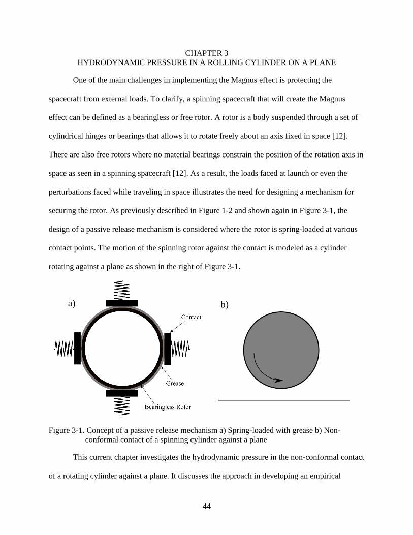
One of the main challenges in implementing the Magnus effect is protecting the
spacecraft from external loads. To clarify, a spinning spacecraft that will create the Magnus
effect can be defined as a bearingless or free rotor. A rotor is a body suspended through a set of
cylindrical hinges or bearings that allows it to rotate freely about an axis fixed in space [12].
There are also free rotors where no material bearings constrain the position of the rotation axis in
space as seen in a spinning spacecraft [12]. As a result, the loads faced at launch or even the
perturbations faced while traveling in space illustrates the need for designing a mechanism for
securing the rotor. As previously described in Figure 1-2 and shown again in Figure 3-1, the
design of a passive release mechanism is considered where the rotor is spring-loaded at various
contact points. The motion of the spinning rotor against the contact is modeled as a cylinder
rotating against a plane as shown in the right of Figure 3-1.
Figure 3-1. Concept of a passive release mechanism a) Spring-loaded with grease b) Non-
conformal contact of a spinning cylinder against a plane
This current chapter investigates the hydrodynamic pressure in the non-conformal contact
of a rotating cylinder against a plane. It discusses the approach in developing an empirical
a) b)

45
relationship for the pressure field as a function of the cylinder’s rotational speed and film
thickness. The empirical relationship is then compared with an analytical solution to examine the
differences in the pressure field. The analytical solution is solved with the parabolic film
thickness approximation which allows one to develop analytical solutions for the pressure.
However, as described by Brewe et al [36], there is some error inherent in the parabolic film
thickness approximation, which increases for thicker film thicknesses. A literature review is
done to examine references that have used the parabolic film thickness approximation in solving
for the pressure distribution and the governing equations for lubrication theory is reviewed.
Furthermore, the rotor will be coated with a shear thinning aerospace grease and as a
result, a Non-Newtonian model is developed for Braycote 601. The Non-Newtonian model is
then implemented into a dynamic mesh simulation to examine the deflection of the cylinder
based on the empirical and parabolic relationship.
Parabolic Approximation
In tribology, a minimum film thickness, h, is used to solve for the pressure distribution
and governs how the film thickness is changing as a function of x (or in the rolling direction) and
is based on the geometry of the rotating surface. For example, for a rolling cylinder on a plane,
the exact film thickness shape takes the form of a circle. However, in order to derive analytical
equations for the pressure, a parabolic film thickness approximation is used which is shown in
Figure 3-2. The motivation is that the film thickness for a cylindrical element, can geometrically
be approximated as a parabola when the lubrication region is sufficiently less than the curvature
of the rotating body or when x << r resulting in x2/r2 <<1. However, as it will be discussed in the
literature review, the parabolic approximation can result in an overestimate of the minimum film
thickness for thicker films as the minimum film thickness h0 increases [37]. These errors could
be significant in designing mechanisms for high-precision applications including those for

46
spaceflight. Hence, examining the differences associated with the parabolic approximation for a
non-conformal contact will be beneficial for future studies in designing a mechanism to contain
the Magnus rotor.
Figure 3-2. Parabolic film thickness approximation for a rolling cylinder on a plane.
Literature Review Using Parabolic Film Thickness Approximation
Sources in literature that have used the parabolic film thickness approximation in solving
for the pressure distribution for a rolling cylinder or sphere will now be briefly reviewed. Snidle
and Archard [38] developed a classical solution for a lubricated sphere spinning on a curved
surface by using the Reynolds equation. The resulting solution predicted the hydrodynamic
pressure at any position in the lubricant film. Significantly, a parabolic approximation was used
to describe the film thickness for the application of angular contact ball bearings, where the
spinning velocity of the balls can be large resulting in hydrodynamic lubrication.
Dowson et al. [39] investigated the special case of a spinning disc against an ellipsoid.
Reynolds equation was written in finite difference form and was solved numerically using a

47
Gauss-Seidel iterative procedure. Again, a parabolic film shape was used as an approximation,
which Dowson justified by stating: when the effective region of pressure generation normally
occurs within a space in the (x,y) plane of restricted dimensions compared with the principal
radii of curvature (Rx, Ry) it is usually acceptable to adopt a parabolic profile for the surface of
the equivalent ellipsoid.
Furthermore, hydrodynamic equations were derived by Kapitza [40] for viscous flow
when a 2D cylinder is rolling on a plane. Kapitza also assumed a parabolic approximation for the
film thickness and derived equations for the pressure distributions in the lubricating layer when
the viscosity increases exponentially with increasing pressure. As an extension to the analysis,
Kapitza examined the problem of a rolling 3D ball [40] where a parabolic dependence was also
assumed for the film thickness. Deriving the pressure distribution, Kapitza found an expression
for the magnitude of the lifting force and the mechanical power consumed by friction. The
minimum film thickness was also derived, and was based on the assumption that the viscosity
depended exponentially on the pressure.
Brewe et al. [36] compared results of the lift coefficient for a rolling ball using the exact
film-thickness equation instead of the parabolic approximation. A pressure distribution satisfying
the Reynolds equation for a given speed, viscosity, geometry, and film thickness was determined
numerically using a Gauss-Seidel iterative method. The authors demonstrated that the parabolic
approximation resulted in an overestimate of the minimum film thickness of approximately 1.6%
and 0.7% for calculated dimensionless film thicknesses of 10-4 and 10-5, respectively. These
overestimates may be important for high precision applications of non-conformal rolling-element
bearings.

48
Thus, examining state of the art methods for lubrication of a rolling cylinder or sphere, it
is seen that the dependence on assuming a parabolic film approximation is common. This part of
the thesis aims to use CFD simulations to derive an empirical relationship for the pressure
distribution for a rolling cylinder based on the full circular film and compare results that use a
parabolic film approximation. Having an understanding of how the pressure from the parabolic
approximation differs from using the full circular film can help one know when to use the
parabolic film. For example, in designing high precision applications the error from the parabolic
approximation for thicker films may be of some tribological significance.
Fluid-Film Lubrication Theory
The objective of the lubricant in machine components is to separate the surfaces in
motion thereby reducing friction and wear leading to longer operating life. The regimes of
lubrication for bearings are divided into four categories including: hydrodynamic,
elastohydrodynamic, mixed, and boundary lubrication. In hydrodynamic lubrication, the
generated pressure is not large enough to cause a significant elastic deformation of the surfaces
and the film thickness normally exceeds 10-6 m. Lubricant films are significantly thicker than the
surface roughness and the physical properties of the lubricant dictate contact behavior. It is the
ideal form of lubrication since it provides low friction and high resistance to wear [13]. In
elastohydrodynamic lubrication, the pressures become on the order of 1 GPa and elastic
deformation of the lubricated surfaces become significant. Moreover, in boundary lubrication the
surfaces are not separated by a lubricant and there is considerable asperity contact. Finally, in a
mixed lubrication regime, a partial fluid film lubrication develops while some contact occurs
between the asperities [13]. The analysis conducted here for a rolling cylinder assumes a
hydrodynamic lubrication regime and thus the film thickness investigated is greater than
7.65x10⁻⁵ m.

49
Governing Equations
In fluid mechanics, the fluid’s pressure and velocity distributions are governed by the
continuity and Navier-Stokes equation shown in Eq. (3-1) and (3-2),
∇. 𝐯 = 0 (3-1)
𝜌 [𝜕
𝜕𝑡𝐯] + (𝐯 ∙ ∇)𝐯 = −∇p + 𝐟𝐛𝐨𝐝𝐲 + 𝜇∇2𝐯
(3-2)
where v is the velocity field, 𝜌 is the lubricant density, 𝜇 is the lubricant viscosity, p is the
pressure between the lubricating surfaces, and 𝑓𝑏𝑜𝑑𝑦 is a body force which is negligible for this
study. Density variations in the lubricant film are sufficiently small, and as a result
incompressible flow is assumed.
As a result of the hydrodynamic regime assumption, isoviscous-rigid conditions are
assumed and hence elastic deformation of the surfaces are neglected. As previously described,
non-conformal contacts are contacting surfaces where the solid surfaces do not fit well
geometrically as seen in ball bearings and gears [41]. The spinning rotor against the contact
regarding the passive release mechanism in Figure 3-1, can be described as a non-conformal
conjunction. When non-conformal conjunctions are very lightly loaded, the hydrodynamic
pressure is not high enough to cause appreciable elastic deformation of the solid surfaces to
significantly change the lubricant viscosity so the lubrication mode is hydrodynamic [13]. The
low pressures and contact area considered in this thesis is conducted for an assumed preload
force ranging from 1 N to 7500 N. This load range was considered since the objective was to
examine the differences in the pressure when using the parabolic approximation. The system
could face various perturbation forces with varying magnitudes and thus higher load conditions
on the rolling contact will be investigated in future work.

50
Reynolds Equation
The pressure field in the lubricant is commonly characterized by Reynolds equation,
𝜕
𝜕𝑥(
ℎ3
12μ
𝜕𝑝
𝜕𝑥) +
𝜕
𝜕𝑧(
ℎ3
12μ
𝜕𝑝
𝜕𝑧) =
𝑢
2
𝜕ℎ
𝜕𝑥
(3-3)
where h (x,z) is an expression describing the film thickness, u is the surface velocity,
∂ h/ 𝜕x is the rate at which the film thickness is changing along the x-axis, 𝜕p/ 𝜕x is the pressure
gradient along the x-axis, and 𝜕p/ 𝜕z is the pressure gradient along the z-axis. This form of the
equation does not neglect side leakage in the z direction.
It was developed using a reduced form of the Navier-Stokes equations and the continuity
equation, to generate a second order differential equation for the pressure in the narrow,
converging gap [13]. The left hand terms in Eq. (3-3) represent the net flow rates due to pressure
gradients within the lubricated area and the right hand term describes the net entraining flow rate
due to surface velocities. Examining this equation, one can deduce the necessary conditions to
generate hydrodynamic forces in the lubricant to support an applied load. For example, if the
rolling-element is stationary (u = 0), Eq. (3-3) implies that the pressure gradients must be zero.
Likewise, if the pairing surfaces are parallel with respect to each other, resulting in no
eccentricity or 𝜕ℎ/𝜕𝑥 = 0, then no hydrodynamic pressure would be developed. In addition, if
the pairing surfaces are diverging or 𝜕ℎ/𝜕𝑥 > 0, Reynolds equation gives a negative pressure
which suggests that cavitation occurs in this region and the flow is dominated by streamlets and a
vapor-liquid mixture [42]. Therefore, the requirements for the lubricant to support an applied
load are: a convergent wedge, a moving surface, and a sufficiently viscous lubricant.
Solving the full Reynolds differential equation includes analytical solutions to the
complete or restricted equation, solutions in the form of mathematical series, and approximate
solutions by numerical procedures [43]. Analytical solutions are only possible for simple

51
problems. Kaptiza was the first to present analytical solutions to Reynolds equation by using the
parabolic film approximation. No analytical solution exists when using the exact circular film
thickness, which results in Reynolds Equation consisting of a homogenous and particular
solution. More specifically, the homogenous solution is an unknown function of the coordinates
along and transverse to the rolling direction and consequently must be determined numerically.
Vortex and Surface Tension Effects
In bearings, vortex flow may occur before the laminar flow breaks down into turbulence
[13]. Once the inertia terms approach the viscous terms, laminar conditions do not hold and
vortices are formed. To assure proper use of Reynolds equation and accurate computational
modeling, the condition for laminar flow in the lubricant when evaluating Reynolds number is,
Re =𝜌𝑢𝑙0𝜇
(ℎ0
𝑙0)2
< 1 (3-4)
and was calculated for all numerical simulations where 𝑢 is the surface velocity, l0 is the
circumference, and ℎ0 is the central minimum film thickness. In addition, to ensure surface
tension effects were negligible the Weber number, Eq. (3-5), was calculated. Flow in mini-
channels with a diameter between 3000 µm and 200 µm is inertia dominated for Weber numbers
when,
We =𝜌𝑢2𝑙0
𝜎> 11.0
(3-5)
For lower values of We, surface tension becomes more important [44].
Minimum Film Thickness
Regarding the lubrication of a rolling cylinder or sphere against a rigid point contact for
Reynolds equation, a minimum film thickness equation must be used in order to numerically
solve for the pressure distribution. This is represented in Eq. (3-6), which can be expanded by a

52
tailor series [13] to yield Eq. (3-7), and can be approximated to Eq. (3-8) by eliminating higher-
order terms,
ℎ = ℎ0 + 𝑟 − 𝑟 [1 − (𝑥
𝑟)]
1/2
(3-6)
ℎ = ℎ0 +1
2(𝑥2
𝑟) [(1 +
1
4(𝑥
𝑟)2
+1
8(𝑥
𝑟)4
+. . . ] (3-7)
ℎ = ℎ0 +𝑥2
2𝑟
(3-8)
where r is the radius of the ball and x is defined as the variable along the rolling direction.
To clarify, in the lubrication region of a rolling cylinder, the lubrication region will start at a
distance x<<r resulting in x2/r2 <<1 making the higher order terms in Eq. (3-7) negligible. The
resulting Eq. (3-8) is then the parabolic film approximation which was also seen graphically in
Figure 3-2.
Computational Fluid Film Modeling
An important benefit of using numerical methods compared to experimental methods is
the possibility of performing parametric equations [45]. It thus becomes possible to vary one
parameter and to investigate the resulting physics. Thus, the pressure distribution for a rolling
cylinder on a plane is examined using Computational Fluid Dynamics (CFD) by varying the
rotational speed and film thickness. CFD is also used in this thesis because it allows one to
examine the parabolic approximation by coupling of the fluid dynamics and rotor dynamics of
the rolling cylinder.
In many conventional lubrication problems, side leakage (flow in the transverse
direction) can be neglected resulting in analytical solutions to Reynolds equation. The resulting
two-dimensional solutions have a definite value, since they provide information about the
general characteristics of the bearing, which lead to a clear physical picture of the performance

53
of lubricating film [13]. For the similar problem of a rolling cylinder on a plane, Hamrock
presents a one-dimensional integrated form of Reynolds equation for the pressure gradient as a
function of x in [13] as shown in Eq. (3-9),
𝑑𝑝
𝑑𝑥= 6𝑢𝜇
[ℎ − ℎ𝑚]
ℎ3
(3-9)
where 𝜇 is the lubricant viscosity, u is the surface velocity of the cylinder, h is the
equation for the film thickness as a function of x, and hm is the film thickness location where
dp/dx = 0, such as the point of maximum pressure. The film thickness location where the
maximum pressure is located, hm, can be evaluated only if the maximum pressure location, xm,
along the rolling direction is known as shown in Eq. (3-10).
ℎ𝑚 = ℎ0 +𝑥𝑚
2
2𝑟
(3-10)
As a result, CFD post processing was used to determine xm by plotting the pressure distribution
along the wall in the converging gap of the rotating cylinder. A similar example is shown in
Figure 3-4, which illustrates the pressure gradient along the wall. After plotting the pressure
distribution along the wall, the maximum pressure location xm was found.
Thus, the CFD simulations allows one to solve Eq. (3-10) which can then be used with
the parabolic film thickness approximation of Eq. (3-8) to evaluate Eq. (3-9) for the pressure
distribution. Equation (3-9) was solved by symbolic integration in Matlab (R2010a, Mathworks)
to derive the maximum pressure generated in the lubricant film. Please refer to Appendix F for a
full documentation of the code. Equation (3-9) is the conventional analytical form used to
determine the pressure field within the interfacial lubricant film. Pressures from the analytical
model are then compared with the developed empirical equation to compare the differences with
using the parabolic assumption.

54
The overall objective is to develop an empirical model for the pressure distribution in the
converging gap by using CFD to account for the exact film thickness equation and compare with
results from the Reynolds equation which uses the conventional parabolic approximation.
Computational Domain and Boundary Conditions
The two-dimensional computational domain is a rolling cylinder surrounded by a
rectangular box, where the fluid is specified over the entire domain and is commonly referred to
as a ‘fully-flooded’ inlet as shown in Figure 3-3.
Figure 3-3. Computational Domain
To enable “rotation” of the cylinder, a rotating wall boundary condition is used, while all
other surfaces are specified as non-slip walls. The commercial software, ANSYS CFX (Version
14.5), was used to perform all numerical simulations. Grid generation is performed using
ANSYS Workbench, which has robust algorithms for creating and editing computational grids.
While performing these simulations, the mesh discretization at the converging gap of the

55
cylinder and wall were refined since sharp pressure gradients were expected in this region. Field
output data is post-processed in ANSYS CFD-Post, a visualization software tool.
Simulation assumptions include laminar flow, constant viscosity, no-slip at the boundary
faces, isothermal conditions, incompressible fluid, inertia and surface tension forces are
negligible compared with viscous forces; this agrees with the conditions in Reynolds equation.
The lubricant properties derive from Braycote 601, a vacuum compatible lubricant with a base
oil viscosity of 0.54 Pa∙s. The radius of the cylinder is 76.2 mm where the central minimum film
thickness h0 is defined as the smallest distance between the rotating cylinder and the wall as
shown in Figure 3-2. This radius was chosen because designing a passive release mechanism
concept as described previously could first be done on smaller radii which could then be flight
tested on a Cubesat. For example, a 76.2 mm radius fits into the 2U Cubesat form factor
(10x10x20cm), and it is possible that the results for the hydrodynamic pressure can be scaled for
larger radii. Simulations are computed using a High Resolution Scheme [46] at both steady state
and transient conditions and the regime of speeds investigated are between 1000 RPM to 15000
RPM.
Validation of Computational Model
To verify that the computational results were consistent with analytical solutions using a
parabolic approximation at low angular speeds, a test case was first considered. A cylinder with a
rotational speed of 100 RPM with a minimum film thickness of 500 µm was the baseline for the
analysis. As illustrated in Figure 3-4, the pressure gradient along the wall is found to be in good
agreement with the analytical relationship.
Parametric Analysis for Maximum Lubricant Pressure
To develop an empirical relationship, the maximum pressure was then graphed as a
function of the minimum film thickness at various operating speeds as shown in Figure 3-5.
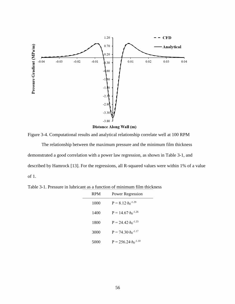
56
Figure 3-4. Computational results and analytical relationship correlate well at 100 RPM
The relationship between the maximum pressure and the minimum film thickness
demonstrated a good correlation with a power law regression, as shown in Table 3-1, and
described by Hamrock [13]. For the regressions, all R-squared values were within 1% of a value
of 1.
Table 3-1. Pressure in lubricant as a function of minimum film thickness
RPM Power Regression
1000 P = 8.12∙h0-1.29
1400 P = 14.67∙h0-1.26
1800 P = 24.42∙h0-1.23
3000 P = 74.30∙h0-1.17
5000 P = 256.24∙h0-1.10

57
Figure 3-5. The maximum pressure in the lubricant film as a function of the minimum film
thickness
After observing the exceptional fit of the power law regression, the power law equations
in Table 3-1 were examined to see if a pattern existed that would allow one to formulate an
equation for the pressure as a function of the minimum film thickness and angular speed. As a
result, this inverse relationship was further investigated by parametrically graphing the
coefficients and exponents of the power law equations as a function of angular speed, as
illustrated in Figure 3-6.
For each speed, five different film thicknesses were used between 76 µm to
1 mm. The coefficients in the power regression exhibited a parabolic relationship
whereas the exponents exhibited a power law relationship as a function of angular speed.
The relationship for the exponent and coefficient regression fit was then substituted into
the power law equation of Table 3-1 resulting in an empirically-derived parametric
equation to predict the pressure as a function of both the minimum film thickness and the
rotation speed. Equation (3-11) is an improved model from the analytical solution

58
because it more accurately represents the geometry of the rotating cylinder, rather than
using a parabolic approximation.
Figure 3-6. A power equation describing the maximum pressure versus the film thickness
contains both a coefficient and exponent term.
The empirical relationship appears to only be valid for speeds greater than 3000 RPM and
deviates for speeds less than 1000 RPM. A possible explanation for this observation is that the
physics at lower speeds is governed by different fluid behavior.
𝑝(ℎ0, 𝜔) = {(1.40𝑥10−5 ∙ 𝜔2 − 2.25𝑥10−2 ∙ 𝜔 + 17.35) ∙ ℎ0
−(2.57∙𝜔−0.098)
𝜔 > 3000 RPM
(3-11)
There is some uncertainty in Equation 3-11 because the uncertainty in the regression coefficients
was not examined.
Computational Solution Versus Analytical Solution
The empirical solution was compared to the analytical solution, and is depicted in Figure
3-8. Angular speed was held constant at 3000 RPM when sweeping through film thicknesses and
then film thickness was held constant at 750 µm when sweeping through angular speeds. The

59
parabolic approximation inherent in the analytical solution deviates from the empirical model
derived from more accurate geometries. For example, as the film thickness increases, there is a
greater difference in maximum pressure because the pressure distribution spreads out more
evenly as opposed to being localized. This effect can be seen more clearly in Figure 3-7 taken
from [36] where the increase in non-dimensional film thickness to 10-4 spreads out more as
opposed to the smaller film thickness of 10-5 which is more concentrated at a point.
Figure 3-7. Pressure profiles along rolling direction for two film thickness.
Thereby, as the pressures spread out more evenly away from the point of minimum film
thickness the parabolic assumption might no longer be valid resulting in greater differences in
hydrodynamic pressure. Also, as the rotational speed increases for a constant film thickness,
there is greater differences in pressure due to the net entraining flow rate of the cylinder.
The empirical and parabolic relationship was further examined by investigating the
pressure field in designing a passive release mechanism for a Magnus rotor configuration
supported by various contacts as shown in Figure 3-9.
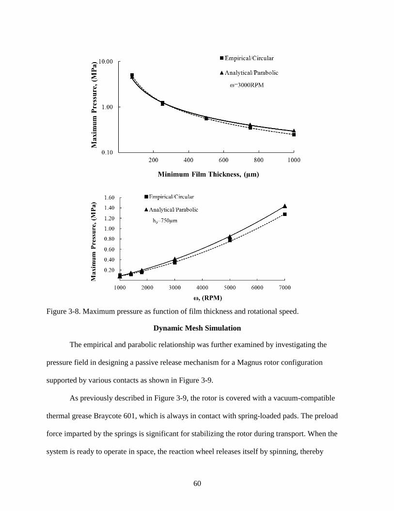
60
Figure 3-8. Maximum pressure as function of film thickness and rotational speed.
Dynamic Mesh Simulation
The empirical and parabolic relationship was further examined by investigating the
pressure field in designing a passive release mechanism for a Magnus rotor configuration
supported by various contacts as shown in Figure 3-9.
As previously described in Figure 3-9, the rotor is covered with a vacuum-compatible
thermal grease Braycote 601, which is always in contact with spring-loaded pads. The preload
force imparted by the springs is significant for stabilizing the rotor during transport. When the
system is ready to operate in space, the reaction wheel releases itself by spinning, thereby

61
generating a pressure field of sufficient intensity to overcome the preload force. For the design
application, the lateral spring is tuned according to the pressure from the analytical relationship,
and also tuned with the empirical model and the resulting deflections from the dynamic
simulations are compared.
Figure 3-9. Spring-loaded passive release mechanism concept for Magnus rotor
Non-Newtonian Model
In order to perform the dynamic mesh simulation for the passive release mechanism, a
Non-Newtonian model was first developed for Braycote 601. This lubricant has been used in the
actuators on the space shuttle and has a strong heritage with the space industry [47]. Depending
on the application, the selection of a lubricant is an important part of designing a bearing unit.
For example, grease is usually preferred for aerospace applications since there is no pressure-
induced outgassing, has exceptional chemical resistance, extremely low volatility, and a wide
temperature service range [48]. In addition, it is good for applications with long operating life, as

62
its base oil degrades very slowly and is usually retained near the contact to continually protect
the bearing surface [49].
Braycote 601 is a non-Newtonian fluid and has a pronounced shear thinning behavior but
maintains a relative important viscosity at high shear rates even or high temperatures [49]. Prat et
al. [49] performed rheological experiments on a controlled high precision shear stress rheometer
for Braycote 601 and determined the apparent viscosity as a function of varying shear rates.
Values of the rheological model parameters for Braycote were then fitted with experimental data
as shown in Figure 3-10 using the Carreau-Yasuda non-Newtonian model,
𝜇 = 𝜇∞ +(𝜇0 − 𝜇∞)
(1 + (𝜆�̇�)𝑎)1−𝑛𝑎
(3-12)
where 𝜇0 is the low shear viscosity, 𝜇∞ is the high shear viscosity, �̇� is the shear strain
rate, a is the yasuda exponent, and 𝜆 is the time constant. The Carreau-Yasuda model is then
implemented into the CFD simulations via the graphical user interface. Simulations comparing
the shear-dependent viscosity versus the isoviscous condition, at various rotational speeds and
varying film thickness, are also shown in the right of Figure 3-10. For the given simulation
parameters, the isoviscous assumption appears to be valid for operating speeds exceeding 1000
RPM, where the percent difference between the Non-Newtonian and isoviscous solution is less
than 5%. During low rotation speeds, the shear dependent model generates a higher maximum
pressure in the converging gap compared to the isoviscous model – this is expected due to the
shear thinning nature of this grease, which is very viscous at low shear rates.
However, as the speed of the cylinder increases, the shear-dependent model approaches
the isoviscous model due to its shear thinning nature, implying that Eq. (3-11) is a valid
approximation for predicting hydrodynamic pressures for a rolling cylinder of radius 76 mm on a

63
plane in a fluid viscosity of 0.54 Pa∙s. Specifically, it can be applied for angular speeds greater
than 3000 RPM with similar shear-thinning lubricant properties as Braycote 601.
Figure 3-10. Braycote experimental data fit and comparing between Non-Newtonian versus
constant viscosity assumption
Design Application Using Empirical Equation
A dynamic mesh simulation, i.e. transient analysis with adaptive remeshing, is used to
demonstrate the case where a lateral spring is imposed on a 2D cylinder and the resulting
deflection is plotted as a function of time. Indeed, models such as this have previously been used,
and it is possible to predict the state of the ball with only a lateral and torsional spring [50]. For
the design application, the lateral spring is tuned according to the pressure from the analytical
relationship, and also tuned with the empirical model. The resulting deflections from the
dynamic simulations are compared. Using CFX’s rigid body modeling features, a linear spring is
placed at the origin of the cylinder to suppress its lift as it rotates counterclockwise at 15000
RPM, as shown in the inset of Figure 3-11. The rigid body solver uses the interacting forces
between the fluid and the rigid body and calculates the motion of the rigid body (or cylinder).
[51]. Mesh motion is used to move the mesh on the rigid body faces in accordance with the
solution of the rigid body equations of motion.

64
Since there is no gravity enabled in the simulation and no other applied load on the
cylinder other than the spring, the rotating cylinder will create a lift force causing it to rise. This
lift force is a function of the cylinder’s speed, geometry, operating viscosity, and minimum film
thickness and can thus be predicted using the empirical model in Eq. (3-11). The lift force and
the spring force will achieve an equilibrium position as the simulation marches forward in time,
resulting in a stable vertical displacement of the cylinder from its original position.
By equating the pressure force to Hooke’s law, the spring constant can be calculated
according to,
𝑘 =𝑝 ∗ 𝐴
ℎ0
(3-13)
where p is the maximum pressure acting on the wall, A is the contact area which is
defined in the subsequent section, and h0 is the central minimum film thickness which is treated
as the spring compression distance. This spring can be used to suppress excessive lift. For the
prescribed computational domain, the minimum film thickness between the cylinder and bottom
wall is initially set at 500 µm. Since the operating speed is within the allowable range for the
developed equation, Eq. (3-11) is used to find the maximum pressure substituting the appropriate
minimum film thickness and angular speed. However, before predicting the lift force, an
expression for the bearing mounting area must be defined.
Contact Area
To estimate a preload spring constant, an expression for the effective ball-to-bearing
interface, i.e., a reasonable area where the spring force would act, was assumed. First, an
expression that locates the maximum pressure for a rolling ball is found in [36], where Brewe et
al. defines an analytical equation based on the work of Kapitza [40],

65
𝑥𝑚 =1
√3√2𝑟𝑎𝑥ℎ0
(3-14)
where ℎ0 is the central minimum film thickness and rax is the radius of curvature of the
ball in the rolling direction. To approximate the area of the contact, both the location of the
maximum pressure, xm and the width of the cylinder, w in the normal plane is required, and is
defined as,
𝐴 = (2 ∙ 𝑥𝑚 ∙ 𝑤) (3-15)
Since this is a 2D simulation, a small width equal to the mesh extrusion length is used for
w. Using the maximum pressure location, the bearing mount area, and the pressure from the
empirical model, a spring constant of 174 kN/m was found, assuming an initial minimum film
thickness of 500 µm. Likewise, solving with the analytical equation yields a spring constant of
183.01 kN/m. In the dynamic mesh simulation, a spring with each of these k values was
implemented separately at the center of the cylinder as illustrated in Figure 3-11. A time step of 1
µs was used to output values for cylinder displacements.
Results from Dynamic Mesh Simulation
Both of the springs from the empirical model and the analytical solution have the
capacity to resist the lift force from the cylinder, and both reached a steady state conditions at 0.8
ms as shown in Figure 3-11. For 15000 RPM there is agreement in the response of the spring
preloaded system using the empirical equation and the analytical solution, with a 4.7% difference
in the deflection. To clarify, there is some uncertainty associated with the empirical equation
since the uncertainty of the regression coefficients were not accounted for. Additional damping
may be considered in future analyses, but requires knowledge of the margin for tolerance,
distortion of the ball, size of particles in lubricant, and heat generation rates [37].

66
Based on Figure 3-11, as the rotational speed increases, the analytical relationship
predicts a higher pressure, resulting in a stiffer spring constant compared to the empirical model.
Subsequently, there is less overshoot in the underdamped system with the analytical solution.
Significantly, as the rotational speed of the cylinder increases, the differences in deflection will
be more noticeably distinct.
Figure 3-11. Design application for a spring loaded ball bearing.
For higher angular speeds, the maximum pressure predicted from the analytical solution,
which uses the parabolic approximation, can result in designing springs that are too stiff. While a
stiff spring will advantageously reduce the deflection of the bearing under maximum load
conditions, at minimum load conditions, the spring may prevent lift-off conditions from
occurring. Correctly calculating bearing stiffness, deflection, or load conditions is critical for
designing for system stability, dynamic loading, and system operation accuracy.

67
Summary of Tribology Study
This part of the thesis investigated the internal flow of a rotating body in a continuum
fluid to aid in the design of a passive release mechanism for the Magnus spacecraft. As a result,
this chapter evaluated the effectiveness of the parabolic film against the exact circular film
thickness approximation on the hydrodynamic pressures for a rolling cylinder on a flat plane.
Reviewing the literature, the parabolic approximation can result in an overestimate of the
minimum film thickness for thicker films which could be significant in designing mechanisms
for high-precision applications including those for spaceflight. An empirical equation based on
the true circular film thickness was developed for the hydrodynamic pressure as a function of
film thickness and rotational speed. This empirical equation was then compared with the
parabolic approximation. It was seen that as the film thickness increased for a constant rotational
speed, there was a greater difference in maximum pressure between the analytical (parabolic) and
empirical (true-circular film) expression as a result of the pressure distribution spreading out more
evenly. The empirical equation results are for a smaller radius and it is possible that it can be
scaled for larger radii.
A design application for designing a passive release mechanism for the Magnus rotor
demonstrated that the influence of the parabolic film thickness approximation may be of some
tribological significance with a 4.7% difference in the deflection of the rolling-element.

68
CHAPTER 4
CONCLUSIONS AND FUTURE RESEARCH
This thesis investigated the internal and external flow of a rotating body to examine the
feasibility of using the Magnus effect to sustain a spacecraft’s orbit. The altitude of apogee, spin
rate, and mass were varied and results demonstrated that the Magnus effect can extend the time
in orbit. This could benefit satellites in LEO in performing in-situ research in the lower
Thermosphere by being a solution strategy in counteracting atmospheric drag. A possible way to
generate the required spin rate could be achieved using reaction wheels or CMG’s.
However, with the Magnus spacecraft, a design challenge is constructing a mechanism to
shield the bearingless rotor from any external disturbances. One possible way to protect the rotor
is to use a passive release mechanism where the rotor is covered in grease and spring-loaded at
various contact points. As a result, the tribology of a rotating cylinder against a plane was
investigated where the parabolic film thickness approximation was compared with an empirically
derived formula based on the true circular film thickness. It was demonstrated that the parabolic
film thickness approximation may be of some tribological significance with a 4.7% difference in
the deflection of the rolling-element.
The Magnus effect seems to be a promising approach for implementation on spacecraft in
meeting the needs of performing research in LEO. However, this was only a feasibility study
examining the magnitude of the Magnus force and one aspect of designing a passive release
mechanism. The results of this thesis warrants further investigation and as a result, a more
detailed design project where other trade-off studies will be performed. For example, an
aerothermal analysis must be performed examining the material selection and the hypersonic air
flow interaction with a spinning satellite. Also, a full description on the hardware requirements
on how to spin a satellite must be conducted including a power budget. Significantly, as the

69
satellite is spinning, the challenge of maintaining communication with the ground station must be
addressed. In addition, the benefit of using reaction wheels as opposed to thrusters to generate
spin must be done. More work must be done in understanding the negative Magnus effect and
the effect of the fluid dynamics in initiating this transition. Regarding the passive release
mechanism, other possible devices to secure the Magnus rotor from external disturbances must
be examined.
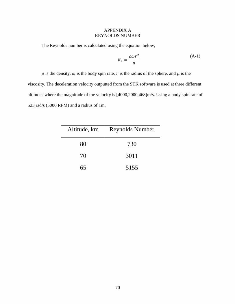
70
APPENDIX A
REYNOLDS NUMBER
The Reynolds number is calculated using the equation below,
𝑅𝑒 =𝜌𝜔𝑟2
𝜇
(A-1)
𝜌 is the density, 𝜔 is the body spin rate, 𝑟 is the radius of the sphere, and 𝜇 is the
viscosity. The deceleration velocity outputted from the STK software is used at three different
altitudes where the magnitude of the velocity is [4000,2000,468]m/s. Using a body spin rate of
523 rad/s (5000 RPM) and a radius of 1m,
Altitude, km Reynolds Number
80 730
70 3011
65 5155

71
APPENDIX B
MAGNUS THRUSTER AXES

72
APPENDIX C
ORBIT ANGULAR MOMENTUM CALCULATION
Body and Orbit Angular Momentum Calculations
Here we perform the calculations for the satellite’s body angular momentum and compare
it with the orbit angular momentum. We perform the calculation for a circular orbit with a semi-
major axis of 6490.59km for a satellite mass of 25kg with a radius of 1m.
Orbit Angular Momentum
Assuming the orbit to be circular the orbital angular momentum can be expressed as,
𝐋 = 𝑚𝑒𝑟2𝜔𝑜𝑟𝑏𝑖𝑡 �̂�
(C-1)
where r is the radius of the orbit and 𝜔𝑜𝑟𝑏𝑖𝑡 is the orbital angular velocity. To find the
orbital angular velocity we use,
𝜔𝑜𝑟𝑏𝑖𝑡 = 2𝜋
𝑇𝑜𝑟𝑏𝑖𝑡
(C-2)
Lastly, to find the period of the orbit or 𝑇𝑜𝑟𝑏𝑖𝑡, we use,
𝑇𝑜𝑟𝑏𝑖𝑡 = 2𝜋√𝑎3
𝜇= 2𝜋√
(6490.59𝑥103𝑚)3
3.98𝑥1014𝑚3
𝑠2
= 5203s (C-3)
As a result, the orbital angular velocity is found to be 0.00120 rad/s. Using Eq. (1) the
orbit angular momentum is found to be,
𝐋 = 25𝑘𝑔 ∙ (6490.59𝑥103𝑚)2 ∙ 0.00120𝑟𝑎𝑑
𝑠= 1.27160𝑥1012 𝑘𝑔 ∙ 𝑚2 ∙ 𝑠−1 �̂�
Body Angular Momentum
We assume we have a spherical satellite and approximate it as a uniform sphere. As a
result, the moment of inertia of the satellite about its center of mass is,

73
𝐼𝑐𝑚 = 2
5𝑚𝑒𝑅𝑒
2 (C-4)
where, 𝑚𝑒 and 𝑅𝑒 is the mass and radius of the satellite. The body angular momentum
can then be found using,
𝐋 = 𝐼 ∙ 𝜔𝑠𝑝𝑖𝑛 =2
5𝑚𝑒𝑅𝑒
2𝜔𝑠𝑝𝑖𝑛 �̂� (C-5)
where �̂� is a unit vector pointing along the axis of rotation of the satellite. Assuming we
are spinning at 5000RPM or 523 rad/s the body angular momentum is found to be,
𝐋 = 𝐼 ∙ 𝜔𝑠𝑝𝑖𝑛 =2
5∙ 25𝑘𝑔 ∙ 1𝑚2 ∙ 523
𝑟𝑎𝑑
𝑠= 5230 𝑘𝑔 ∙ 𝑚2 ∙ 𝑠−1 �̂�

74
APPENDIX D
HYPERBOLIC TANH
function MySmooth () syms x a=82 b=.5 %x=linspace(0,1) f_x= 2 g_x=-4/3 s_x=.5+.5*tanh((x-a)/b) h_x=s_x*g_x+(1-s_x)*f_x f=matlabFunction(h_x) t=linspace(90,80,10)' a=f(t) ezplot(h_x) ezplot(h_x,[80, 90,-2,2.5])
% hold on % ezplot(s_x) % hold on % ezplot(f_x) % hold on % ezplot(g_x)
%test=1/3-(5/3).*(exp((5.*x./6-70000))-exp(-5.*x./6+70000))/(exp(5.*x./6-
70000)+exp(-5.*x./6+70000)) test=1/3-(5/3).*(exp((2.*x-164))-exp(-2.*x+164))/(exp(2.*x-164)+exp(-
2.*x+164))
ezplot(test,[80, 90,-2,2.5]) final_f=matlabFunction(test) v=linspace(180,65);
c=final_f(v)
plot(v,c,'k') axis([65 90 -1.5 2.5 ]) xlabel('Altitude, km') ylabel('Lift Cofficient') end
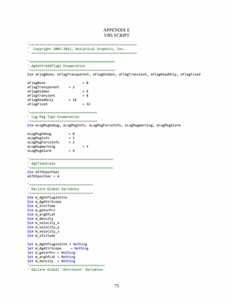
75
APPENDIX E
VBS SCRIPT
'====================================================== ' Copyright 2005-2011, Analytical Graphics, Inc. ' ===================================================== '=========================================== ' AgEAttrAddFlags Enumeration '=========================================== Dim eFlagNone, eFlagTransparent, eFlagHidden, eFlagTransient, eFlagReadOnly, eFlagFixed eFlagNone = 0 eFlagTransparent = 2 eFlagHidden = 4 eFlagTransient = 8 eFlagReadOnly = 16 eFlagFixed = 32 '================================== ' Log Msg Type Enumeration '================================== Dim eLogMsgDebug, eLogMsgInfo, eLogMsgForceInfo, eLogMsgWarning, eLogMsgAlarm eLogMsgDebug = 0 eLogMsgInfo = 1 eLogMsgForceInfo = 2 eLogMsgWarning = 3 eLogMsgAlarm = 4 '========================================== ' AgETimeScale '========================================== Dim eSTKEpochSec eSTKEpochSec = 4 '================================ ' Declare Global Variables '================================ Dim m_AgUtPluginSite Dim m_AgAttrScope Dim m_InitTime Dim m_gatorPrv Dim m_argOfLat Dim m_density Dim m_velocity_x Dim m_velocity_y Dim m_velocity_z Dim m_altitude Set m_AgUtPluginSite = Nothing Set m_AgAttrScope = Nothing Set m_gatorPrv = Nothing Set m_argOfLat = Nothing Set m_density = Nothing '====================================== ' Declare Global 'Attribute' Variables

76
'====================================== Dim m_Name Dim m_T0 Dim m_T1 Dim m_T2 Dim m_Ts Dim m_Tc Dim m_Isp Dim m_radius m_Name = "VBScript.Example1.EngineModel.wsc" m_T0 = 2 m_T1 = 0 m_T2 = 0 m_Ts = 0 m_Tc = 0 m_Isp = 2E12 '======================= ' GetPluginConfig method '======================= Function GetPluginConfig( AgAttrBuilder ) If( m_AgAttrScope is Nothing ) Then 'MsgBox "here1" Set m_AgAttrScope = AgAttrBuilder.NewScope() 'MsgBox "here2" '=========================== ' General Plugin attributes '=========================== Call AgAttrBuilder.AddStringDispatchProperty( m_AgAttrScope, "PluginName", "Human readable plugin name or alias", "Name", eFlagReadOnly ) 'MsgBox "here3" '=========================== ' Propagation related '=========================== Call AgAttrBuilder.AddDoubleDispatchProperty ( m_AgAttrScope, "T0", "Initial Thrust", "T0", 0 ) Call AgAttrBuilder.AddDoubleDispatchProperty ( m_AgAttrScope, "T1", "Linear Thrust Coefficient", "T1", 0 ) Call AgAttrBuilder.AddDoubleDispatchProperty ( m_AgAttrScope, "T2", "Quadratic Thrust Coefficient", "T2", 0 ) Call AgAttrBuilder.AddDoubleDispatchProperty ( m_AgAttrScope, "Ts", "Sine Thrust Coefficient", "TS", 0 ) Call AgAttrBuilder.AddDoubleDispatchProperty ( m_AgAttrScope, "Tc", "Cosine Thrust Coefficient", "TC", 0 ) 'MsgBox "here4" Call AgAttrBuilder.AddDoubleDispatchProperty ( m_AgAttrScope, "Isp", "Specific Impulse", "ISP", 0 ) 'MsgBox "here5" End If 'MsgBox "here6" 'If m_AgAttrScope is Nothing Then ' MsgBox "Uhhh Oh" 'End If Set GetPluginConfig = m_AgAttrScope

77
End Function '=========================== ' VerifyPluginConfig method '=========================== Function VerifyPluginConfig(AgUtPluginConfigVerifyResult) Dim Result Dim Message Result = true Message = "Ok" 'TODO: Add Yaw and Pitch Maximum and Minimum Checks here AgUtPluginConfigVerifyResult.Result = Result AgUtPluginConfigVerifyResult.Message = Message End Function '=========================== ' Message method '=========================== Sub Message( msgType, msg ) If( Not m_AgUtPluginSite is Nothing) then Call m_AgUtPluginSite.Message( msgType, msg ) End If End Sub '====================== ' Init Method '====================== Function Init( AgUtPluginSite ) Set m_AgUtPluginSite = AgUtPluginSite if(NOT m_AgUtPluginSite is Nothing) then Set m_gatorPrv = m_AgUtPluginSite.GatorProvider if(NOT m_gatorPrv is Nothing) then Set m_argOfLat = m_gatorPrv.ConfigureCalcObject("Argument_of_Latitude") Set m_density = m_gatorPrv.ConfigureCalcObject("AtmosDensity") Set m_velocity_x=m_gatorPrv.ConfigureCalcObject("Vx") Set m_velocity_y=m_gatorPrv.ConfigureCalcObject("Vy") Set m_velocity_z=m_gatorPrv.ConfigureCalcObject("Vz") Set m_altitude=m_gatorPrv.ConfigureCalcObject("Altitude") end if end if if(m_argOfLat is Nothing) then Init = 0 else Init = 1 end if ' if(m_density is Nothing) then 'Init = 0 'else 'Init = 1 'end if

78
End Function '====================== ' PrePropagate Method '====================== Function PrePropagate( AgGatorPluginResultState ) If( Not AgGatorPluginResultState is Nothing) then Dim dcArray dcArray = AgGatorPluginResultState.DayCount_Array( eStkEpochSec ) If(IsArray(dcArray) and UBound(dcArray) > 0) Then m_InitTime = dcArray(0) * 86400.0 + dcArray(1) End If End If PrePropagate = 1 End Function '====================== ' PreNextStep Function '====================== Function PreNextStep( AgGatorPluginResultState ) PreNextStep = 1 End Function '================= ' Evaluate Method '================= Function Evaluate( AgGatorPluginResultEvalEngineModel ) If( Not AgGatorPluginResultEvalEngineModel is Nothing) then Dim time Dim Thrust Dim deltaT Dim argOfLat Dim dcArray Dim argOfDen Dim argOfVelx Dim argOfVely Dim argOfVelz Dim VecMag Dim argOfAlt Dim cL Dim altKm time = m_InitTime dcArray = AgGatorPluginResultEvalEngineModel.DayCount_Array( eStkEpochSec ) If(IsArray(dcArray) and UBound(dcArray) > 0) Then time = dcArray(0) * 86400.0 + dcArray(1) End If deltaT = time - m_InitTime argOfLat = m_argOfLat.Evaluate(AgGatorPluginResultEvalEngineModel) argOfDen = m_density.Evaluate(AgGatorPluginResultEvalEngineModel)

79
argOfVelx = m_velocity_x.Evaluate(AgGatorPluginResultEvalEngineModel) argOfVely = m_velocity_y.Evaluate(AgGatorPluginResultEvalEngineModel) argOfVelz = m_velocity_z.Evaluate(AgGatorPluginResultEvalEngineModel) argOfAlt = m_altitude.Evaluate(AgGatorPluginResultEvalEngineModel) VecMag= Sqr( ( ( argOfVelx) )^2 + ( ( argOfVely ) )^2 + ( ( argOfVelz ) )^2) ''argOfTank= 'Thrust = m_T0 + m_T1 * deltaT + m_T2 * deltaT^2 + m_Ts * sin(argOfLat) + m_Tc * cos(argOfLat) 'Assuming Radius=.34m, with 500RPM 'Thrust=4.308405*Abs(VecMag)*Abs(argOfDen) altKm=argOfAlt/1000 'If altitude is under 80km we are in a continuum regime where Cl=2. Assuming radius is 1m with 5000RPM we get: 'cL=67/200-(333/200)*(Exp(altKm-80) - Exp(-altKm+80)) / (Exp(altKm-80) + Exp(-altKm+80)) if (abs(altKm)<=100) then '(1/2)*pi*radius^3*5000 RPM*V*rho*Cl '17RPM (1.78 rad/s) 'cL=1/3-(5/3)*(Exp(2*altKm-164) - Exp(-2*altKm+164)) / (Exp(2*altKm-164) + Exp(-2*altKm+164)) 'Thrust=.5*3.14*1*1.78*Abs(VecMag)*Abs(argOfDen)*Abs(cL) '5000 RPM cL=1/3-(5/3)*(Exp(2*altKm-164) - Exp(-2*altKm+164)) / (Exp(2*altKm-164) + Exp(-2*altKm+164)) Thrust=.5*3.14*1*523.6*Abs(VecMag)*Abs(argOfDen)*Abs(cL) '10000 RPM 'Thrust=.5*3.14*1*1047.197*Abs(VecMag)*Abs(argOfDen)*Abs(cL) 'cL=1/3-(5/3)*(Exp(2*altKm-164) - Exp(-2*altKm+164)) / (Exp(2*altKm-164) + Exp(-2*altKm+164)) 'Thrust=1644.93*Abs(VecMag)*Abs(argOfDen)*Abs(cL) '15000 RPM 'Thrust=.5*3.14*1*1570.79*Abs(VecMag)*Abs(argOfDen)*Abs(cL) 'cL=1/3-(5/3)*(Exp(2*altKm-164) - Exp(-2*altKm+164)) / (Exp(2*altKm-164) + Exp(-2*altKm+164)) 'Thrust=2467.4005*Abs(VecMag)*Abs(argOfDen)*Abs(cL) else '17 RPM (1.78 rad/s) 'Thrust=.5*3.14*1*1.78*Abs(VecMag)*Abs(argOfDen)*(4/3) 'Thrust=3.728*Abs(VecMag)*Abs(argOfDen) '5000 RPM 'Thrust=.5*3.14*1*1570.79*Abs(VecMag)*Abs(argOfDen)*(4/3) Thrust=1096.624*Abs(VecMag)*Abs(argOfDen) '10000 RPM (1570.79 rad/s)

80
'Thrust=.5*3.14*1*1047.197*Abs(VecMag)*Abs(argOfDen)*(4/3) 'Thrust=2193.244*Abs(VecMag)*Abs(argOfDen) '15000 RPM (1570.79 rad/s) 'Thrust=.5*3.14*1*1570.79*Abs(VecMag)*Abs(argOfDen)*(4/3) 'Thrust=3289.867*Abs(VecMag)*Abs(argOfDen) end if '---------------------------------------------------------------------- Call AgGatorPluginResultEvalEngineModel.SetThrustAndIsp(Thrust, m_Isp) End If Evaluate = 1 End Function '================= ' Free Method '================= Sub Free() ' do nothing End Sub '================== ' Name property '================== Function GetName() GetName = m_Name End function '================== ' T0 property '================== Function GetT0() GetT0 = m_T0 End Function Function SetT0( thrust ) m_T0 = thrust End Function '================== ' T1 property '================== Function GetT1() GetT1 = m_T1 End Function Function SetT1( thrust ) m_T1 = thrust End Function '================== ' T2 property '================== Function GetT2() GetT2 = m_T2 End Function Function SetT2( thrust ) m_T2 = thrust End Function '================== ' TS property '================== Function GetTS()
81
GetTS = m_Ts End Function Function SetTS( thrust ) m_Ts = thrust End Function '================== ' TC property '================== Function GetTC() GetTC = m_Tc End Function Function SetTC( thrust ) m_Tc = thrust End Function '================== ' ISP property '================== Function GetISP() GetISP = m_Isp End Function Function SetISP( isp ) m_Isp = isp End Function '====================================================== ' Copyright 2005-2011, Analytical Graphics, Inc. ' =====================================================

82
APPENDIX F
MATLAB CODE FOR HYDRODYNAMIC PRESSURE
Integrating Hamrocks 1-D Equation
x=[7.62E-04 3.81E-04 7.62E-05 3.81E-05]
y=[-0.0273719 -0.0310457 -0.048746 -0.0567153 ]
plot (x,y)
clc;clear all num2=xlsread('pressure_25000RPM.csv') x_pressure=num2(:,1) p=num2(:,2)
%Graphing Pressure Gradient num=xlsread('pressuregrad_25000RPM.csv') %Reading in Pressure Gradient Values xgrad=num(:,1) Pgrad=num(:,2)
r=0.0762; %Radius of Sphere x1=-0.04 %Domain Extents x2=0.04 x=linspace(-100,100) m=.54; %Base Oil Viscosity %Minimum Film Thickness ho=5E-04; w_rpm=25000 w=w_rpm*(2*pi)/60 U=w*r;
%Joining x and pressure together to get location of maximum pressure C=[x_pressure p]; %Finding the maximum Pressure pmax=max(C(:,2))
format long %Finding the maximum pressure (col 2) and finding the corresponding index xIndex = find(C(:,2) == max(C(:,2)), 1, 'first'); format long %The maximum pressure location is equal to the value of xindex maxXValue = x_pressure(xIndex) xm=maxXValue
syms X Xm %Use the parabolic approximation because it is easier to integrate H=ho+X^2/(2*r) Hm=ho+Xm^2/(2*r) %Redefining pressure gradient with symbols so we can integrate it dpdx=6*U*m*((H-Hm)./H.^3)

83
x_new=linspace(-.04,.04,75) dpdx2=subs(dpdx,Xm,xm)
f_dpdx=matlabFunction(dpdx2) y=f_dpdx(xgrad)
plot(xgrad,y) hold on plot(xgrad,Pgrad) f=int(dpdx) f=subs(f,Xm,xm)
% ezplot(f) %xplot=linspace(x1,x2) %we make the symbolic expression a function handle so it is easier to work %with P_sol=matlabFunction(f) %Integrated in terms of xm and x and now we sub in xm value from before
x_expand=linspace(x1,x2,75) y2=P_sol(xgrad)%we evaluate analytical function at x_pressure values fprintf('Maximum value of analytical pressure is %f\n and CFD solution is
%f',max(y2),max(p)) plot(xgrad,y2,xgrad,p)
Empirical Equation
clc clear all format longG h=9.73E-5 %rpm=5000 %rpm=[20 50 100 500 1000 1400 1800 3000 5000 7000 3628.73]' rpm=[3000 5000 7000 8000]' %h=[1.00E-03 7.50E-04 5.00E-04 2.50E-04 7.62E-05]'
%rpm=3 P_Eq= (5.58156E-05*h.^-1.79401).*rpm.^(2.02*h.^0.07155) % % RPM>1000 P_fast_1000RPM=(0.0000140553.*rpm.^2 - 0.0225671.*rpm + 17.3473).*h.^(-
1*(2.57099*(rpm.^-0.09823)))
P_500RPM= (1.22042E-05.*rpm.^2 - 1.06154E-02.*rpm + 2.53438).*h.^(-
1*(2.41328.*rpm.^-0.09018))
r=.0762 %width=0.0508%2inch width=0.00152476 %width=.0254 length=4*((1/sqrt(3))*sqrt(2*r*h)) A=length*width k=P_fast_1000RPM*A/h

84
F=5 P=F/A % % k_excel=205295*A/h
85
LIST OF REFERENCES
[1] "QB50 The Project," [Online]. Available: https://www.qb50.eu/index.php/project-
description-obj. [Accessed 12 October 2016].
[2] G. R. Karr, "Analysis of Satellite Drag and Spin Decay Data, UAH Report No.456," The
University of Alabama, Huntsville, 1985.
[3] M. N. Goodson, "Applications of Aerodynamic Forces for Spacecraft Orbit
Maneuverability in Opereationally Responsive Space and Space Reconstitution Needs,"
Air Force Institure of Technology, Ohio, 2012.
[4] J. Wertz, Space Mission Design and Analysis, 3rd ed., Torrence, CA: Microcosm, Chaps.
5,6,8, 1999.
[5] J. Wertz, Space Mission Engineering: The New SMAD, Microcosm Press, 2011.
[6] A.-A. L. C. Cojuangco, "Orbital Lifetime Analysis of PICO- and NANO-satellites,"
University of Florida, Gainesville , 2007.
[7] S. R. Omar, "Using Differential Aerodynamic Forces for Cubesat Orbit Control," Auburn
University Journal of Undergraduate Scholarship , Spring 2014.
[8] J. Borg, "Magnus Effect: An Overview of its Past and Future Practical Applications,"
NAVSEA , Washington D.C., 1986.
[9] K. I. Borg, L. H. Soderholm and H. Essen, "Force on a Spinning Sphere Moving in a
Rarefied Gas," Physics of Fluids, vol. 15, no. 3, pp. 736-741, 2003.
[10] M. Emanuelli and T. Sgobba, "Assessing the Aviation Risk from Space Debris and
Meteoroids," Space Safety Magazine, no. 8, pp. 24-25, 2013, Summer.
[11] M. Garcia, "Space Debris and Human Spacecraft," NASA, 27 July 2016. [Online].
Available: http://www.nasa.gov/mission_pages/station/news/orbital_debris.html.
[Accessed 15 November 2016].
[12] G. Genta, Dynamics of Rotating Systems, New York: Springer, 2005.
[13] B. Hamrock, Fundamentals of Fluid Film Lubrication, Washington D.C.: NASA, 1991.
[14] H.-S. Tsien, "Superaerodynamics, Mechanics of Rarefied Gases," Journal of the
Aeronautical Sciences, vol. 13, no. 12, pp. 653-664, 1946.

86
[15] H.-S. Tsien, "Superaerodynamics, Mechanics of Rarefied Gases," Journal of the
Aeronautical Sciences, vol. 13, no. 12, pp. pp. 653-664, 1946.
[16] A. Volkov, "Aerodynamic coefficients of a Spinning Sphere in a Rarefied-Gas Flow,"
Izvestiya Rossiiskoi Akademii Nauk, vol. 44, no. 1, pp. 167-187, 2009.
[17] G. E. Cook, "The Effect of Aerodynamic Lift on Satellite Orbit," Plant. Space Science ,
vol. 12, p. 11, 1964.
[18] J. Storch, "Aerodynamic Disturbances on Spacecraft in Free-Molecular Flow," Aerospace
Corporation, TR-2003(3397)-1, Los Angeles Air Force Base, 2002.
[19] K. Moe, M. M. Moe and S. D. Wallace, "Improved Satellite Drag Coefficient Calculations
from Orbital Measurements of Energy Accommodation," Journal of Spacecraft and
Rockets, vol. 35, no. 3, pp. 266-272, 1998.
[20] G. E. Cook and R. Plimmer, "The Effect of Atmospheric Rotation on the Orbital Plane of a
Near-Earth Satellite," in Proceedings of the Royal Society of London. Series A,
Mathematical and Physical Sciences , Farnborough, 196.
[21] J. Ashenberg, "On the Effects of Time-Varying Aerodynamics Coefficients on Satellite
Orbits," Acta Astronautica , vol. 38, no. 2, pp. 75-86, 1996.
[22] P. Moore, "The Effect of Aerodynamic Lift on Near-Circular Satellite Orbits," Planet,
Space Sciences , vol. 33, no. 5, pp. 479-491, 1985.
[23] S. Roy, R. Raju, H. F. Chuang, B. A. Cruden and M. Meyyappan, "Modelng Gas Flow
Through Microchannels and Nanopores," Journal of Applied Physics , vol. 93, no. 8, p. 10,
2003.
[24] C.-T. Wang, Free Molecular Flow Over a Rotating Sphere, Lafayette: AIAA, 1972.
[25] S. I. Rubinow and J. B. Keller, "The Transverse Force on a Spinning Sphere Moving in a
Viscous Fluid," Journal of Fluid Mechanics , vol. 11, no. 3, p. 12, 1961.
[26] T. S. Hall, "Orbit Maneuver for Responsive Coverage using Electric Propulsion," Air
Force Institute of Technology, Ohio, 2010.
[27] J. R. Wertz and W. J. Larson, SMAD, El Segundo : Microcosm Press, 2003.
[28] V. Chobotov, Orbital Mechanics Second Edition, Reston, Virginia : American Institutre of
Aeronautics and Astronautics , 1996.

87
[29] AGI, "STK 11.0.1 Programming Interface," AGI, [Online]. Available:
http://help.agi.com/stkdevkit/index.html?page=source%2FSTKPlugins%2FenginePlugins_
engineExtensibility.htm.
[30] C.-T. Want, "Free Molecular Flow Over a Rotating Sphere," AIAA, 1972.
[31] S. Roy, R. Raju, H. F. Chuang, B. A. Cruden and M. Meyyappan, "Modeling gas flow
through microchannels and nanopores," Journal of Applied Physics, vol. 93, no. 8, p. 10,
2003.
[32] G. Elliott, C. Granger and A. Timmermann, Handbook of Economic Forecasting, Elsevier:
North Holland, 2006.
[33] Analytical Graphics Inc., "STK Programming Interface," October 2013.
[34] Blue Canyon Technologies , "Reaction Wheels," 2015. [Online]. Available:
http://bluecanyontech.com/wp-content/uploads/2016/07/RW.pdf. [Accessed 18 August
2016].
[35] HoneyBee Robotics Spacecraft Mechanisms Corporation , "Microsat CMG Attitude
Control Array," [Online]. Available: http://www.honeybeerobotics.com/wp-
content/uploads/2014/03/Honeybee-Robotics-Microsat-CMGs.pdf. [Accessed 18 August
2016].
[36] D. E. Brewe, B. J. Hamrock and C. M. Taylor, "Effect of Geometery on Hydrodynamic
Film Thickness," NASA, Virginia, 1978.
[37] B. Hamrock and D. Dowson, "Applications of Film Thickness Equations," NASA
Technical Memorandum 81701, 1983.
[38] R. Snidle and J. Archard, "Theory of Hydrodynamic Lubrication for a Spinning Sphere," in
Proc Instn Mech Engrs , Leicester, 1969-70.
[39] D. Dowson, C. Taylor and H. Xu, "The Lubrication of Elliptical Contacts with Spin,"
Proceedings of the Institution of Mechanical Engineers Part C Journal of Mechanical
Engineering Science , Vols. 203-210, pp. 165-174, 1993.
[40] P. Kapitza, Collected Papers of Kapitza, London: Pergamon Press, 1965.
[41] B. J. Hamrock, "Lubrication Fundamentals," NASA Technical Memorandum 81762,
Cleveland, Ohio, 1981.

88
[42] M. He, C. H. Cloud and J. M. Byrne, "Fundamentals of Fluid Film Journal Bearing
Operation and Modeling," in Proceedings of the Thirty-Fourth Turbomachinery
Symposium , 2005.
[43] D. Dowson, History of Tribology, New York: Longman Inc, 1979.
[44] C. T. Clayton , Multiphase Flow Handbook, Taylor and Francis, 2006.
[45] T. Almqvist, "Computational Fluid Dynamics in Theoretical Simulations of
Elastohydrodynamic Lubrication," Louisiana State University, Baton Rouge, 2004.
[46] "ANSYS CFX-Solver Theory Guide," ANSYS Inc., Canonsburg, 2012.
[47] M. Buttery, "An Evaluation of Liquid, Solid, and Grease Lubricants for Space Mechanisms
Using a Spiral Orbit Tribometer," in Proceedings of the 40th Aerospace Mechanisms
Symposium,, NASA Kennedy Space Center, 2010.
[48] "Castrol Braycote 601 EF," Structure Probe, Inc./SPI Supplies, [Online]. Available:
http://www.2spi.com/catalog/vac/braycote-601EF-properties.html. [Accessed 29 May
2015].
[49] P. Prat, M. Vergne, M. Pochard and J. Sicre, "Optimisation of the Rheological Behavior of
Thickened Liquid Lubricants for Spacecraft Applications," in Lubricants and Lubrication,
1995.
[50] T. A. Harris, Rolling Bearing Analysis, New York: John Wiley & Sons, 2001.
[51] ANSYS Inc., "Chapter 22: Modeling a Ball Check Valve Using Mesh Deformation and the
CFX Rigid Body Solver," ANSYS Inc..

89
BIOGRAPHICAL SKETCH
Sahadeo Ramjatan was born in Guyana, South America and moved to the United States
at a young age with his family. He completed his Associate of Arts in engineering at Valencia
College in 2010 and subsequently graduated with his Bachelor of Science in Aerospace
Engineering from the University of Florida in Spring 2014. He received his Master of Science in
aerospace engineering at the University of Florida in December 2016 under the guidance of Dr.
Norman Fitz-Coy. He performed a summer semester working with the Applied Physics Research
Group at UF under the guidance of Dr. Subrata Roy. He performed two internships at NASA
Goddard Spaceflight Center under the guidance of Dr. Alvin Yew and was recognized as a 2015
John Mather Nobel Scholar for high academic achievement in the aerospace field. He also
performed an internship at the Von Karman Institute for Fluid Dynamics in Belgium
investigating the hypersonic radio blackout phenomena. His main interests are in the field of
fluid dynamics and he is a recent attendee of the 66th Lindau Nobel Laureate Meeting in Lindau,
Germany. At the University of Florida, he is part of the Space Systems Group advised by Prof.
Norman Fitz-Coy.