Analysis of a High Temperature Supercritical BraytonCycle for Space Exploration

Ian M. Rousseau

under the direction of

Professor Michael DriscollMassachusetts Institute of Technology

Nuclear Engineering Department

Research Science Institute

July 31, 2007

Abstract

This paper provides a preliminary analysis of the supercritical Brayton cycle, a power

generation system for space exploration. Supercritical working fluids increase efficiency due

to increased compressibility at the critical point but have not been investigated at the high

temperatures necessary for space power generation. Through computer simulation, the vi-

ability of the supercritical Brayton cycle is verified for space exploration. Several working

fluids are evaluated. Results show efficiency increases of 221% over the sodium Rankine

cycle and 105% over thermoelectric conversion. For future cycles at 1600 K, sulfur is the

best working fluid. Given present materials constraints, iodine is the best fluid at 1200 K.

1 Introduction

The purpose of this paper is to perform a preliminary analysis of high temperature super-

critical Brayton cycles as it pertains to space exploration. Simple Brayton cycles have been

explored for space exploration, but they are not as efficient as condensing cycles. Since su-

percritical fluids have properties of both liquids and gases, performing compression around

the critical point increases efficiency. Supercritical Brayton cycles have been designed at an

operating temperature of 650 K, but the concept has not carried over to space exploration,

which requires temperatures over 1000 K. This paper provides a thermodynamic preliminary

analysis of several supercritical working fluids and proves the viability of the supercritical

Brayton cycle for space exploration.

1.1 Background

Humans have walked on the moon and sights are now set on manned Mars exploration,

but physiological limitations of the human body in zero gravity prohibit prolonged space

missions. Current travel time to Mars with conventional propulsion is at a minimum of nine

months each way. In order to shorten travel time to three months, manned Mars exploration

requires spacecraft velocities ranging from 40 to 100 km/second. Conventional chemical

rockets will not be able to power manned missions at these velocities [9].

Electric ion propulsion is a promising propulsion system for future space exploration. An

electric field charges and ejects atoms of a noble gas (xenon or krypton). A 25 kW prototype

of an electric xenon ion system achieved more than fifteen times the efficiency of today’s best

chemical rockets [21]. To go to Mars and beyond, 100-400 kW thrusters are needed [25].

Currently, there is no way to fulfill an electric ion thrusters’ power requirements in space.

Solar cell arrays are heavy and would not receive enough sunlight in deep space. A small

nuclear fission reactor (less than 1 MW) would meet this power requirement, but reactor

1

thermal energy needs to be processed by power converters to create electric power.

There are two methods to extract electrical energy from the thermal energy of nuclear

reactions. Static conversion uses no moving parts to generate DC power. This method is

ideally suited for space flight because the absence of moving parts negates the possibility

of mechanical failure. However, static conversion methods are currently limited in total

power output, efficiency, and mass. Thermionic converters, thermophotovoltaic cells, and

thermoelectric converters are examples of static conversion 1.

Dynamic power conversion (heat cycles) converts thermal energy into AC power. Ther-

mal energy is transferred to a working fluid. The fluid is compressed and heated before being

sent through a turbine, which is linked to a generator. Although dynamic conversion may

be more complex than static methods, heat cycles are scalable and the technology is ma-

ture; coal, nuclear, wood, and gas powerplants use heat cycles. Dynamic power conversion

methods include the Stirling, Rankine, Carnot, Otto, and Brayton cycles 2. Of these, only

the Brayton cycle is ideally suited for space because its simplicity decreases the likelihood

of mechanical failure.

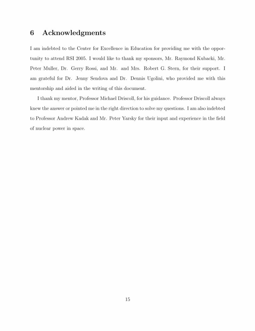
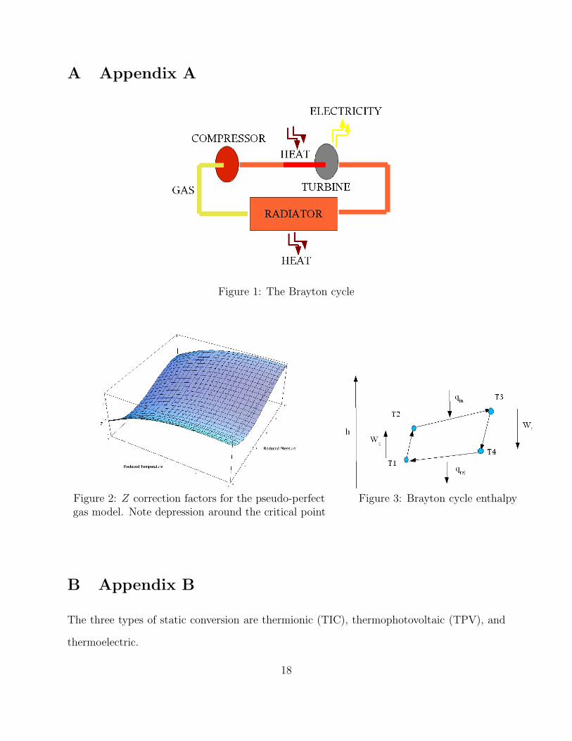
Simple Brayton cycles function much like closed circuit jet engines with near-ideal gases.

First, the gas is compressed via a compressor linked to the turbine. Next, heat is added

to increase gas enthalpy. The hot, high pressure gas is sent through a turbine to generate

electricity. Finally, the gas releases thermal energy in the radiator before beginning the

cycle again (Figure 1; See Appendix A). A helium Brayton cycle for terrestrial power plants

achieved 43% efficiency at 1073 K [8]. By comparison, today’s best coal power plants are

35-40% efficient [17].

Heat cycles in space present a major difficulty. Since there is no matter in space, radiation

is the sole option for releasing thermal energy. The gray body heat radiation, Qrej, is defined

1Information about static converison methods can be found in Appendix B.2See [3] for information about heat cycles.

2

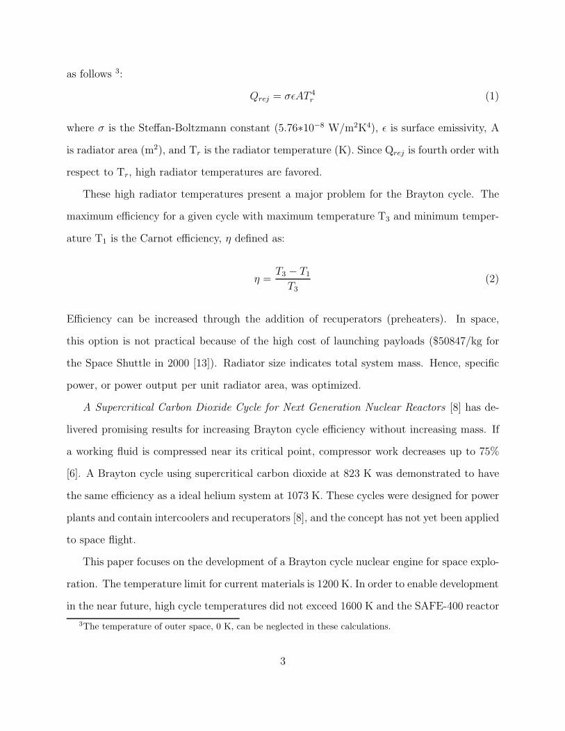
as follows 3:

Qrej = σεAT 4r (1)

where σ is the Steffan-Boltzmann constant (5.76∗10−8 W/m2K4), ε is surface emissivity, A

is radiator area (m2), and Tr is the radiator temperature (K). Since Qrej is fourth order with

respect to Tr, high radiator temperatures are favored.

These high radiator temperatures present a major problem for the Brayton cycle. The

maximum efficiency for a given cycle with maximum temperature T3 and minimum temper-

ature T1 is the Carnot efficiency, η defined as:

η =T3 − T1

T3(2)

Efficiency can be increased through the addition of recuperators (preheaters). In space,

this option is not practical because of the high cost of launching payloads ($50847/kg for

the Space Shuttle in 2000 [13]). Radiator size indicates total system mass. Hence, specific

power, or power output per unit radiator area, was optimized.

A Supercritical Carbon Dioxide Cycle for Next Generation Nuclear Reactors [8] has de-

livered promising results for increasing Brayton cycle efficiency without increasing mass. If

a working fluid is compressed near its critical point, compressor work decreases up to 75%

[6]. A Brayton cycle using supercritical carbon dioxide at 823 K was demonstrated to have

the same efficiency as a ideal helium system at 1073 K. These cycles were designed for power

plants and contain intercoolers and recuperators [8], and the concept has not yet been applied

to space flight.

This paper focuses on the development of a Brayton cycle nuclear engine for space explo-

ration. The temperature limit for current materials is 1200 K. In order to enable development

in the near future, high cycle temperatures did not exceed 1600 K and the SAFE-400 reactor

3The temperature of outer space, 0 K, can be neglected in these calculations.

3

was used. The SAFE-400, a standard reactor in theoretical nuclear spacecraft design, is a

400 kW highly enriched uranium fission reactor operating at 1250 K. Supercritical working

fluids were used to increase cycle efficiency. Working fluid selection optimized power output

per unit radiator area.

2 Methods and Materials

2.1 Working Fluid Selection

Working fluid selection was based on several criteria. First, the fluid’s critical point must

fall within a given range, 800-1400 K. If the critical temperature (Tc) is too low, radiator

mass increases according to the gray body radiation equation (Equation 1). If the critical

temperature is too high, efficiency and power output drop according to Carnot efficiency

(Equation 2). Corrosion properties of the supercritical fluid are considered. For space

missions, system reliability and low mass are the foremost goals. Exotic and expensive

materials are employed in an effort to increase performance.

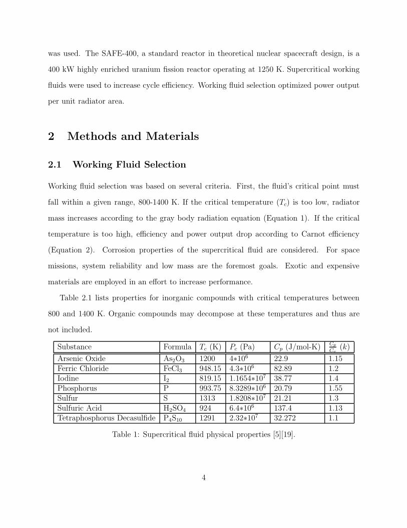
Table 2.1 lists properties for inorganic compounds with critical temperatures between

800 and 1400 K. Organic compounds may decompose at these temperatures and thus are

not included.

Substance Formula Tc (K) Pc (Pa) Cp (J/mol-K) Cp

Cv(k)

Arsenic Oxide As2O3 1200 4∗106 22.9 1.15Ferric Chloride FeCl3 948.15 4.3∗106 82.89 1.2Iodine I2 819.15 1.1654∗107 38.77 1.4Phosphorus P 993.75 8.3289∗106 20.79 1.55Sulfur S 1313 1.8208∗107 21.21 1.3Sulfuric Acid H2SO4 924 6.4∗106 137.4 1.13Tetraphosphorus Decasulfide P4S10 1291 2.32∗107 32.272 1.1

Table 1: Supercritical fluid physical properties [5][19].

4

2.1.1 Supercritical Fluid Model

Supercritical fluids cannot be modeled as ideal gases around the critical point [6]. Experi-

mental data is used to determine supercritical properties, but high temperature supercritical

fluid data was unavailable. Properties of the gases were determined based on available for-

mulas. The specific heat, Cp, was either found in a reference table [19] or calculated from a

formula [5] at the average cycle temperature. The ratio of specific heats, k, is dependent on

both the number of atoms per molecule and the molar mass of the fluid. A reference table

was used to estimate k values [7].

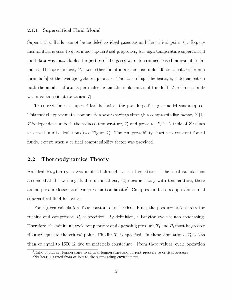
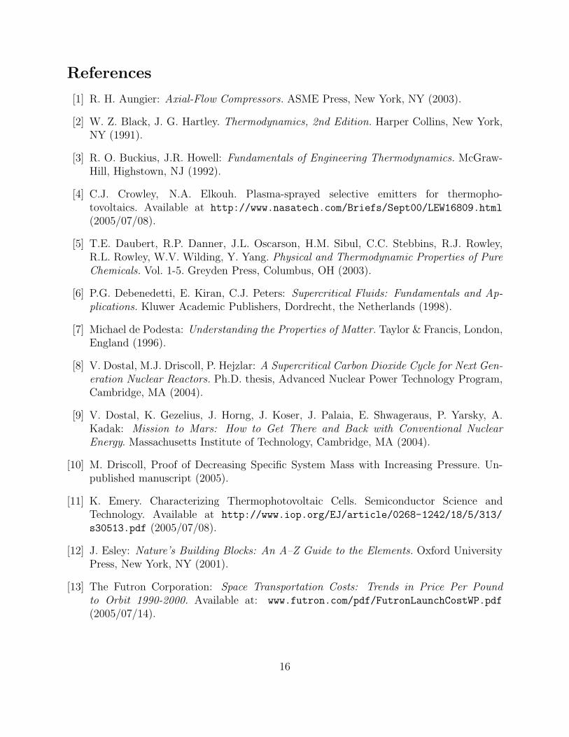
To correct for real supercritical behavior, the pseudo-perfect gas model was adopted.

This model approximates compression works savings through a compressibility factor, Z [1].

Z is dependent on both the reduced temperature, Tr and pressure, Pr4. A table of Z values

was used in all calculations (see Figure 2). The compressibility chart was constant for all

fluids, except when a critical compressibility factor was provided.

2.2 Thermodynamics Theory

An ideal Brayton cycle was modeled through a set of equations. The ideal calculations

assume that the working fluid is an ideal gas, Cp does not vary with temperature, there

are no pressure losses, and compression is adiabatic5. Compression factors approximate real

supercritical fluid behavior.

For a given calculation, four constants are needed. First, the pressure ratio across the

turbine and compressor, Rp is specified. By definition, a Brayton cycle is non-condensing.

Therefore, the minimum cycle temperature and operating pressure, T1 and P1 must be greater

than or equal to the critical point. Finally, T3 is specified. In these simulations, T3 is less

than or equal to 1600 K due to materials constraints. From these values, cycle operation

4Ratio of current temperature to critical temperature and current pressure to critical pressure5No heat is gained from or lost to the surrounding environment.

5

parameters are calculated.

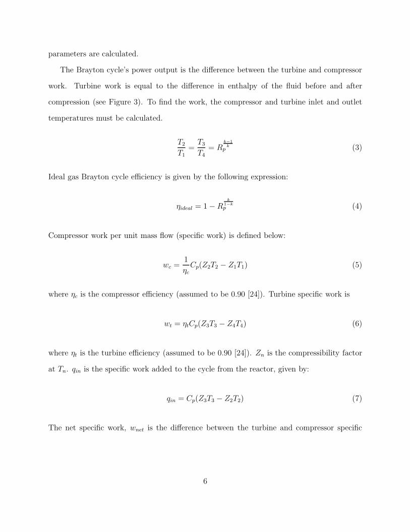
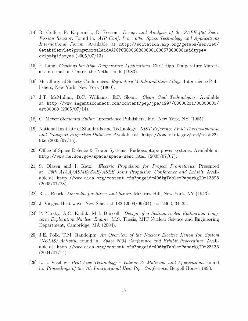
The Brayton cycle’s power output is the difference between the turbine and compressor

work. Turbine work is equal to the difference in enthalpy of the fluid before and after

compression (see Figure 3). To find the work, the compressor and turbine inlet and outlet

temperatures must be calculated.

T2

T1=

T3

T4= R

k−1k

p (3)

Ideal gas Brayton cycle efficiency is given by the following expression:

ηideal = 1 − Rk

1−kp (4)

Compressor work per unit mass flow (specific work) is defined below:

wc =1

ηcCp(Z2T2 − Z1T1) (5)

where ηc is the compressor efficiency (assumed to be 0.90 [24]). Turbine specific work is

wt = ηtCp(Z3T3 − Z4T4) (6)

where ηt is the turbine efficiency (assumed to be 0.90 [24]). Zn is the compressibility factor

at Tn. qin is the specific work added to the cycle from the reactor, given by:

qin = Cp(Z3T3 − Z2T2) (7)

The net specific work, wnet is the difference between the turbine and compressor specific

6

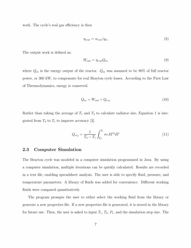
work. The cycle’s real gas efficiency is then

ηreal = wnet/qin (8)

The output work is defined as:

Wout = ηrealQin (9)

where Qin is the energy output of the reactor. Qin was assumed to be 80% of full reactor

power, or 360 kW, to compensate for real Brayton cycle losses. According to the First Law

of Thermodynamics, energy is conserved.

Qin = Wout + Qrej (10)

Rather than taking the average of T1 and T4 to calculate radiator size, Equation 1 is inte-

grated from T4 to T1 to improve accuracy [3].

Qrej =1

T4 − T1

∫ T1

T4

σεAT 4dT (11)

2.3 Computer Simulation

The Brayton cycle was modeled in a computer simulation programmed in Java. By using

a computer simulation, multiple iterations can be quickly calculated. Results are recorded

in a text file, enabling spreadsheet analysis. The user is able to specify fluid, pressure, and

temperature parameters. A library of fluids was added for convenience. Different working

fluids were compared quantitatively.

The program prompts the user to either select the working fluid from the library or

generate a new properties file. If a new properties file is generated, it is stored in the library

for future use. Then, the user is asked to input T1, T3, P1, and the simulation step size. The

7

simulation increments the pressure ratio by the step size until a maximum pressure ratio is

reached (5 in these simulations), performing calculations at each step. The calculations are

recorded in a formatted text file.

Since the compressibility table contains no formula for calculating intermediate values,

an estimation algorithm had to be adopted. Global regressions generalize local extrema,

and were discarded. The table was in three dimensions, further complicating calculations.

To estimate intermediate values, the four vertices around the point were found. Two linear

regressions were performed at constant pressure. These two points were used to perform a

linear regression at constant temperature, yielding a compressibility value.

3 Results

Simulations were run at two temperatures. High temperature (1600 K) simulations were

run for each fluid to simulate potential future Brayton cycles. 1200 K tests were run to

simulate supercritical Brayton cycles that could be implemented today. 1200 K is close

to the heat pipe outlet temperature of the SAFE-400 reactor, 1250 K [14]. The 1600 K

cycle would require a higher outlet temperature reactor. Fluids not included in the 1200 K

simulations did not produce cycles with positive work output. In the tables,“I” refers to ideal

gas efficiency, while “R” refers to compressibility corrected efficiency. All other calculations

are for corrected gas behavior. Table values were optimum specific power values for each

fluid. If the specific power calculation diverged, optimum specific work values were chosen.

If specific work diverged, then the calculation with an pressure ratio of 2.25 was selected.

8

9

10

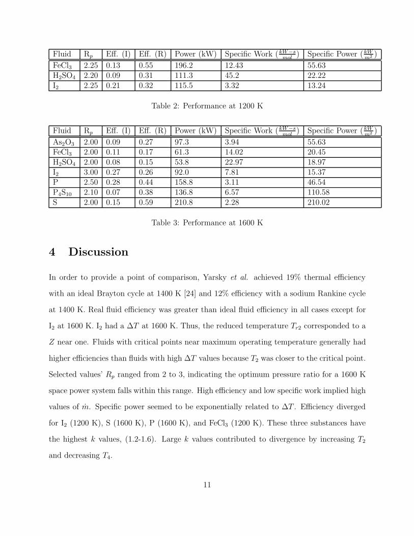
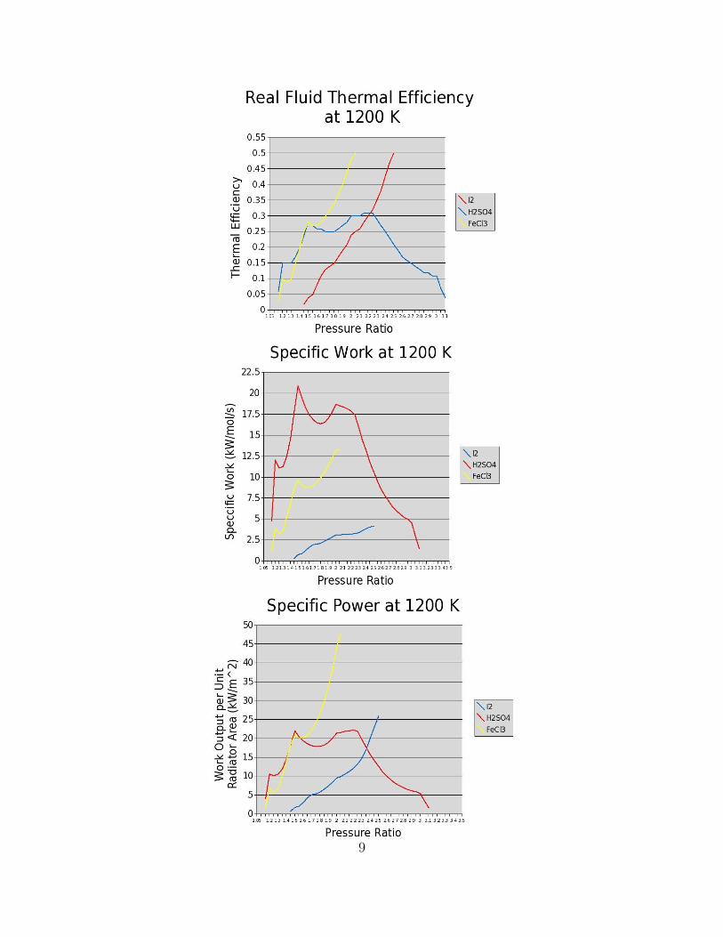
Fluid Rp Eff. (I) Eff. (R) Power (kW) Specific Work (kW−smol

) Specific Power (kWm2 )

FeCl3 2.25 0.13 0.55 196.2 12.43 55.63H2SO4 2.20 0.09 0.31 111.3 45.2 22.22I2 2.25 0.21 0.32 115.5 3.32 13.24

Table 2: Performance at 1200 K

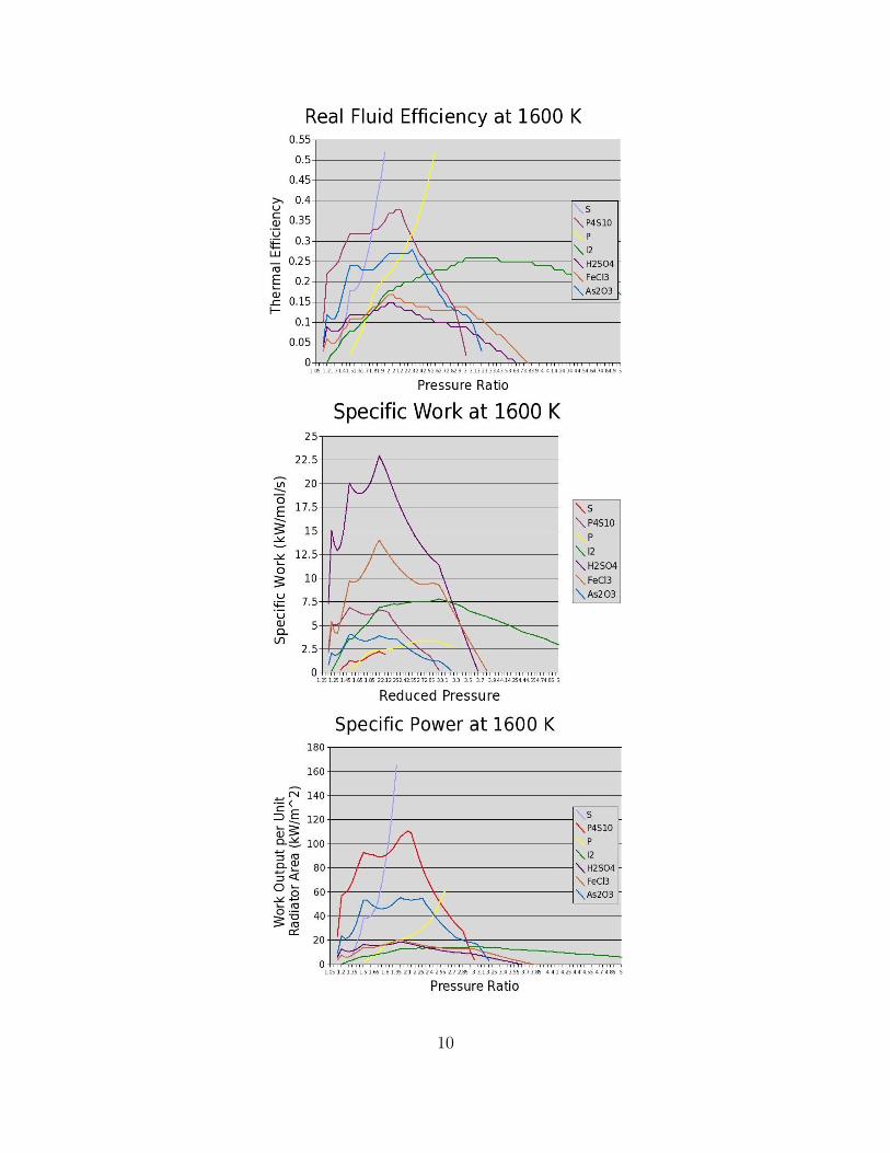
Fluid Rp Eff. (I) Eff. (R) Power (kW) Specific Work (kW−smol

) Specific Power (kWm2 )

As2O3 2.00 0.09 0.27 97.3 3.94 55.63FeCl3 2.00 0.11 0.17 61.3 14.02 20.45H2SO4 2.00 0.08 0.15 53.8 22.97 18.97I2 3.00 0.27 0.26 92.0 7.81 15.37P 2.50 0.28 0.44 158.8 3.11 46.54P4S10 2.10 0.07 0.38 136.8 6.57 110.58S 2.00 0.15 0.59 210.8 2.28 210.02

Table 3: Performance at 1600 K

4 Discussion

In order to provide a point of comparison, Yarsky et al. achieved 19% thermal efficiency

with an ideal Brayton cycle at 1400 K [24] and 12% efficiency with a sodium Rankine cycle

at 1400 K. Real fluid efficiency was greater than ideal fluid efficiency in all cases except for

I2 at 1600 K. I2 had a ∆T at 1600 K. Thus, the reduced temperature Tr2 corresponded to a

Z near one. Fluids with critical points near maximum operating temperature generally had

higher efficiencies than fluids with high ∆T values because T2 was closer to the critical point.

Selected values’ Rp ranged from 2 to 3, indicating the optimum pressure ratio for a 1600 K

space power system falls within this range. High efficiency and low specific work implied high

values of m. Specific power seemed to be exponentially related to ∆T . Efficiency diverged

for I2 (1200 K), S (1600 K), P (1600 K), and FeCl3 (1200 K). These three substances have

the highest k values, (1.2-1.6). Large k values contributed to divergence by increasing T2

and decreasing T4.

11

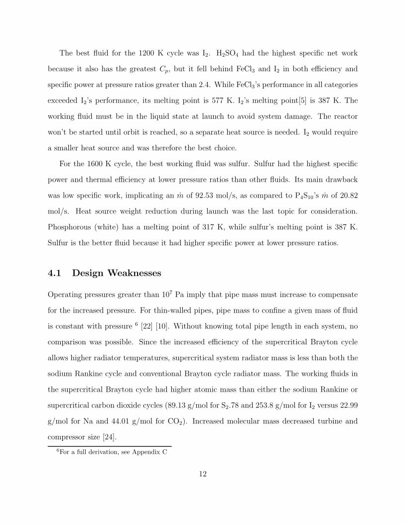
The best fluid for the 1200 K cycle was I2. H2SO4 had the highest specific net work

because it also has the greatest Cp, but it fell behind FeCl3 and I2 in both efficiency and

specific power at pressure ratios greater than 2.4. While FeCl3’s performance in all categories

exceeded I2’s performance, its melting point is 577 K. I2’s melting point[5] is 387 K. The

working fluid must be in the liquid state at launch to avoid system damage. The reactor

won’t be started until orbit is reached, so a separate heat source is needed. I2 would require

a smaller heat source and was therefore the best choice.

For the 1600 K cycle, the best working fluid was sulfur. Sulfur had the highest specific

power and thermal efficiency at lower pressure ratios than other fluids. Its main drawback

was low specific work, implicating an m of 92.53 mol/s, as compared to P4S10’s m of 20.82

mol/s. Heat source weight reduction during launch was the last topic for consideration.

Phosphorous (white) has a melting point of 317 K, while sulfur’s melting point is 387 K.

Sulfur is the better fluid because it had higher specific power at lower pressure ratios.

4.1 Design Weaknesses

Operating pressures greater than 107 Pa imply that pipe mass must increase to compensate

for the increased pressure. For thin-walled pipes, pipe mass to confine a given mass of fluid

is constant with pressure 6 [22] [10]. Without knowing total pipe length in each system, no

comparison was possible. Since the increased efficiency of the supercritical Brayton cycle

allows higher radiator temperatures, supercritical system radiator mass is less than both the

sodium Rankine cycle and conventional Brayton cycle radiator mass. The working fluids in

the supercritical Brayton cycle had higher atomic mass than either the sodium Rankine or

supercritical carbon dioxide cycles (89.13 g/mol for S2.78 and 253.8 g/mol for I2 versus 22.99

g/mol for Na and 44.01 g/mol for CO2). Increased molecular mass decreased turbine and

compressor size [24].

6For a full derivation, see Appendix C

12

Special materials have to be considered for construction of this high temperature Brayton

cycle. There are three options for materials: refractory metals, ceramic coatings, and oxide

strengthened steels. Materials must avoid corrosion at these temperatures. Exotic ceramic

coatings, such as TaN, B4C, HfC, ZrN, BN, or HfN can withstand operating temperatures

greater than 1000 K [15]. Refractory metals such as columbium, molybdenum, tantalum,

tungsten, and their alloys display oxidation resistance at temperatures greater than 1000 K

[16]. Oxide strengthened steels are capable of withstanding these temperatures, but corrosion

compatibilities with supercritical I2 and S need to be determined. Some combination of these

substances may yield a satisfactory working material.

Objections will be raised about the use of toxic chemicals as working fluids. At high

temperatures, however, any material is dangerous. For example, supercritical steam is ex-

tremely corrosive at 800 K. Citing precedent, H2SO4, I2, and S are currently used for large

scale hydrogen production at 1273 K. Plutonium has already been launched into orbit for the

Cassini mission [20]. The SAFE-400, a highly enriched uranium reactor, will not be started

until it is in orbit. With the reliability of today’s launch vehicles, risk is mitigated. Since

operation is in space, a pressure leak will pose no threat to the environment.

5 Conclusions

The pseudo-perfect gas model (Law of Corresponding States) proves the viability of the

supercritical Brayton cycle based on both efficiency and weight reduction. At 1600 K, the

best working fluid is sulfur. If limited by current materials constraints at 1200 K, the best

working fluid is I2. High temperature supercritical Brayton cycles deserve further theoretical

and experimental research.

13

5.1 Further Work

The simulation needs improvement to more closely model real supercritical fluids and a real

Brayton cycle. The next step is use of generalized enthalpy and entropy charts instead of

compressibility values. Since a real Brayton cycle is not isothermal, using constant Cp is an

approximation. For I2, Cp increases by 1.7% on the temperature interval from 800 K to 1200

K and 5.9% between 800 K and 1600 K. Ideal Brayton cycle equations must be integrated

over the operational temperature range to estimate the real Brayton cycle. A method for

estimating total system mass must be adopted.

Physical properties of high temperature supercritical fluids must be experimentally mea-

sured. These measurements should provide the basis for a supercritical fluid model. Cor-

rosion properties of working fluids at these high temperatures should be determined. Many

working fluids, such as sulfur and phosphorus, have unique properties that may alter physical

and corrosion properties at temperatures greater than 1000 K. Sulfur gas is a mixture of S8,

S7, S6, S5, S4, S3, S2, and S1. At the critical point, there are 2.78 atoms per molecule [5].

With increasing temperature, this number decreases [18]. Phosphorus has three allotropes,

red, white, and black phosphorus. The melting point of red phophorus is 870 K, while the

melting point of white phosphorus is 317 K. White phosphorus is much more reactive than

either red or black phosphorus. Allotrope abundance in supercritical fluids is unknown.

Current materials constraints limit maximum cycle temperature to 1200 K [19]. New

materials should be developed to withstand high temperatures, possibly allowing high cycle

temperatures up to 1600 K. Additionally, eutectics, mixtures of fluids, could provide working

fluids with intermediate properties. A pressure leak in a space heat cycle would be catas-

trophic. Small diameter heat pipes could be used to increase robustness. A heat pipe uses

capillary action to move fluids. Heat pipe performance in zero gravity environments and

with supercritical fluids needs to be studied [26] [9].

14

6 Acknowledgments

I am indebted to the Center for Excellence in Education for providing me with the oppor-

tunity to attend RSI 2005. I would like to thank my sponsors, Mr. Raymond Kubacki, Mr.

Peter Muller, Dr. Gerry Rossi, and Mr. and Mrs. Robert G. Stern, for their support. I

am grateful for Dr. Jenny Sendova and Dr. Dennis Ugolini, who provided me with this

mentorship and aided in the writing of this document.

I thank my mentor, Professor Michael Driscoll, for his guidance. Professor Driscoll always

knew the answer or pointed me in the right direction to solve my questions. I am also indebted

to Professor Andrew Kadak and Mr. Peter Yarsky for their input and experience in the field

of nuclear power in space.

15

References

[1] R. H. Aungier: Axial-Flow Compressors. ASME Press, New York, NY (2003).

[2] W. Z. Black, J. G. Hartley. Thermodynamics, 2nd Edition. Harper Collins, New York,NY (1991).

[3] R. O. Buckius, J.R. Howell: Fundamentals of Engineering Thermodynamics. McGraw-Hill, Highstown, NJ (1992).

[4] C.J. Crowley, N.A. Elkouh. Plasma-sprayed selective emitters for thermopho-tovoltaics. Available at http://www.nasatech.com/Briefs/Sept00/LEW16809.html

(2005/07/08).

[5] T.E. Daubert, R.P. Danner, J.L. Oscarson, H.M. Sibul, C.C. Stebbins, R.J. Rowley,R.L. Rowley, W.V. Wilding, Y. Yang. Physical and Thermodynamic Properties of PureChemicals. Vol. 1-5. Greyden Press, Columbus, OH (2003).

[6] P.G. Debenedetti, E. Kiran, C.J. Peters: Supercritical Fluids: Fundamentals and Ap-plications. Kluwer Academic Publishers, Dordrecht, the Netherlands (1998).

[7] Michael de Podesta: Understanding the Properties of Matter. Taylor & Francis, London,England (1996).

[8] V. Dostal, M.J. Driscoll, P. Hejzlar: A Supercritical Carbon Dioxide Cycle for Next Gen-eration Nuclear Reactors. Ph.D. thesis, Advanced Nuclear Power Technology Program,Cambridge, MA (2004).

[9] V. Dostal, K. Gezelius, J. Horng, J. Koser, J. Palaia, E. Shwageraus, P. Yarsky, A.Kadak: Mission to Mars: How to Get There and Back with Conventional NuclearEnergy. Massachusetts Institute of Technology, Cambridge, MA (2004).

[10] M. Driscoll, Proof of Decreasing Specific System Mass with Increasing Pressure. Un-published manuscript (2005).

[11] K. Emery. Characterizing Thermophotovoltaic Cells. Semiconductor Science andTechnology. Available at http://www.iop.org/EJ/article/0268-1242/18/5/313/

s30513.pdf (2005/07/08).

[12] J. Esley: Nature’s Building Blocks: An A–Z Guide to the Elements. Oxford UniversityPress, New York, NY (2001).

[13] The Futron Corporation: Space Transportation Costs: Trends in Price Per Poundto Orbit 1990-2000. Available at: www.futron.com/pdf/FutronLaunchCostWP.pdf

(2005/07/14).

16

[14] R. Guffee, R. Kapernick, D. Poston: Design and Analysis of the SAFE-400 SpaceFission Reactor. Found in: AIP Conf. Proc. 608: Space Technology and ApplicationsInternational Forum. Available at http://scitation.aip.org/getabs/servlet/

GetabsServlet?prog=normal&id=APCPCS000608000001000578000001&idtype=

cvips&gifs=yes (2005/07/13).

[15] E. Lang: Coatings for High Temperature Applications. CEC High Temperature Materi-als Information Center, the Netherlands (1983).

[16] Metallurgical Society Conferences: Refractory Metals and their Alloys. Interscience Pub-lishers, New York, New York (1960).

[17] J.T. McMullan, B.C. Williams, E.P. Sloan: Clean Coal Technologies. Availableat: http://www.ingentaconnect.com/content/pep/jpe/1997/00000211/00000001/

art00008 (2005/07/14).

[18] C. Meyer:Elemental Sulfur. Interscience Publishers, Inc., New York, NY (1965).

[19] National Institute of Standards and Technology: NIST Reference Fluid Thermodynamicand Transport Properties Database. Available at: http://www.nist.gov/srd/nist23.htm (2005/07/15).

[20] Office of Space Defence & Power Systems. Radioisoptope power systems. Available athttp://www.ne.doe.gov/space/space-desc.html (2005/07/07).

[21] S. Olasen and I. Katz: Electric Propulsion for Project Prometheus. Presentedat: 39th AIAA/ASME/SAE/ASEE Joint Propulsion Conference and Exhibit. Avail-able at: http://www.aiaa.org/content.cfm?pageid=406&gTable=Paper&gID=13898

(2005/07/28).

[22] R. J. Roark: Formulas for Stress and Strain. McGraw-Hill, New York, NY (1943).

[23] J. Viegas. Heat wave. New Scientist 182 (2004/09/04), no 2463, 34–35.

[24] P. Yarsky, A.C. Kadak, M.J. Driscoll: Design of a Sodium-cooled Epithermal Long-term Exploration Nuclear Engine. M.S. Thesis, MIT Nuclear Science and EngineeringDepartment, Cambridge, MA (2004).

[25] J.E. Polk, T.M. Randolph: An Overview of the Nuclear Electric Xenon Ion System(NEXIS) Activity. Found in: Space 2004 Conference and Exhibit Proceedings. Avail-able at: http://www.aiaa.org/content.cfm?pageid=406&gTable=Paper&gID=23133

(2004/07/14).

[26] L. L. Vasiliev: Heat Pipe Technology – Volume 2: Materials and Applications. Foundin: Proceedings of the 7th International Heat Pipe Conference. Bergell House, 1993.

17

A Appendix A

Figure 1: The Brayton cycle

Figure 2: Z correction factors for the pseudo-perfect Figure 3: Brayton cycle enthalpygas model. Note depression around the critical point

B Appendix B

The three types of static conversion are thermionic (TIC), thermophotovoltaic (TPV), and

thermoelectric.

18

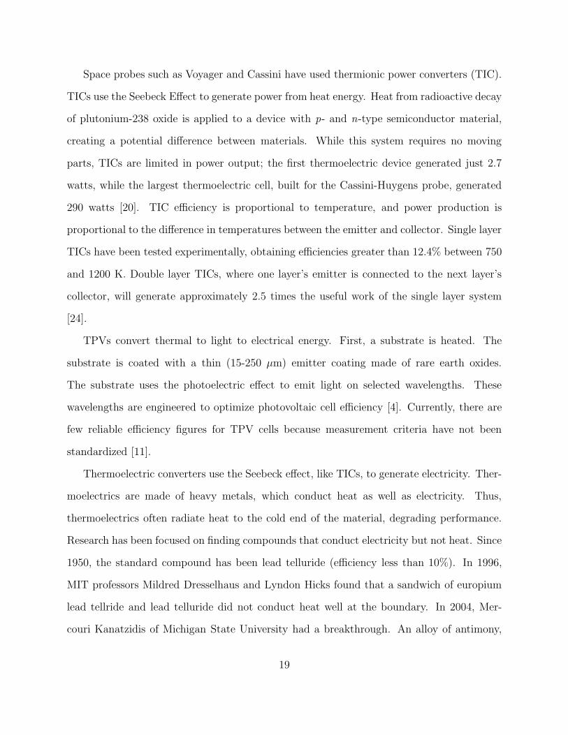
Space probes such as Voyager and Cassini have used thermionic power converters (TIC).

TICs use the Seebeck Effect to generate power from heat energy. Heat from radioactive decay

of plutonium-238 oxide is applied to a device with p- and n-type semiconductor material,

creating a potential difference between materials. While this system requires no moving

parts, TICs are limited in power output; the first thermoelectric device generated just 2.7

watts, while the largest thermoelectric cell, built for the Cassini-Huygens probe, generated

290 watts [20]. TIC efficiency is proportional to temperature, and power production is

proportional to the difference in temperatures between the emitter and collector. Single layer

TICs have been tested experimentally, obtaining efficiencies greater than 12.4% between 750

and 1200 K. Double layer TICs, where one layer’s emitter is connected to the next layer’s

collector, will generate approximately 2.5 times the useful work of the single layer system

[24].

TPVs convert thermal to light to electrical energy. First, a substrate is heated. The

substrate is coated with a thin (15-250 µm) emitter coating made of rare earth oxides.

The substrate uses the photoelectric effect to emit light on selected wavelengths. These

wavelengths are engineered to optimize photovoltaic cell efficiency [4]. Currently, there are

few reliable efficiency figures for TPV cells because measurement criteria have not been

standardized [11].

Thermoelectric converters use the Seebeck effect, like TICs, to generate electricity. Ther-

moelectrics are made of heavy metals, which conduct heat as well as electricity. Thus,

thermoelectrics often radiate heat to the cold end of the material, degrading performance.

Research has been focused on finding compounds that conduct electricity but not heat. Since

1950, the standard compound has been lead telluride (efficiency less than 10%). In 1996,

MIT professors Mildred Dresselhaus and Lyndon Hicks found that a sandwich of europium

lead tellride and lead telluride did not conduct heat well at the boundary. In 2004, Mer-

couri Kanatzidis of Michigan State University had a breakthrough. An alloy of antimony,

19

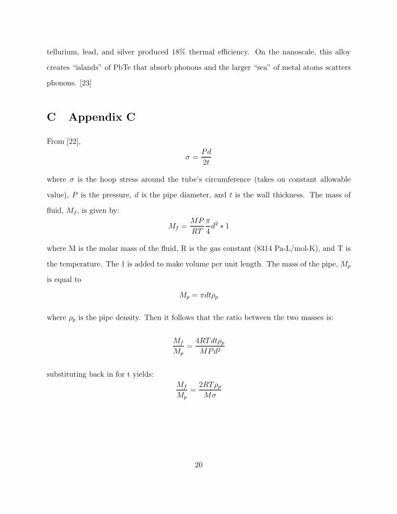
tellurium, lead, and silver produced 18% thermal efficiency. On the nanoscale, this alloy

creates “islands” of PbTe that absorb phonons and the larger “sea” of metal atoms scatters

phonons. [23]

C Appendix C

From [22],

σ =Pd

2t

where σ is the hoop stress around the tube’s circumference (takes on constant allowable

value), P is the pressure, d is the pipe diameter, and t is the wall thickness. The mass of

fluid, Mf , is given by:

Mf =MP

RT

π

4d2 ∗ 1

where M is the molar mass of the fluid, R is the gas constant (8314 Pa-L/mol-K), and T is

the temperature. The 1 is added to make volume per unit length. The mass of the pipe, Mp

is equal to

Mp = πdtρp

where ρp is the pipe density. Then it follows that the ratio between the two masses is:

Mf

Mp=

4RTdtρp

MPd2

substituting back in for t yields:

Mf

Mp=

2RTρp

Mσ

20