Embed Size (px)
Citation preview
Analysis III

December 22, 2018.

Contents
Chapter 1. Preface 1
Chapter 2. The Laplace Transform 32.1. Introduction 32.2. Definitions and examples 32.3. First properties and applications 52.3.1. Linearity 52.3.2. Shifting Theorem (s-shifting) 62.3.3. Differentiation 72.4. The Heaviside function and t-shifting 82.4.1. Second shifting theorem (t-shifting) 102.5. Integration 122.6. Dirac’s delta function 142.7. Convolution and integral equations 172.8. Last properties: differentiation and integration of transforms 20
Chapter 3. Fourier Analysis 233.1. Fundamentals 233.2. Even and odd functions, half-range expansion 303.2.1. Simplified form of the Fourier series for even and for odd functions 303.2.2. The half-range expansion 323.3. Complex Fourier series 353.4. Approximation by trigonometric polynomials 383.5. Fourier integral 393.5.1. Fourier sine and Fourier cosine integrals 413.6. Fourier transform 42
Chapter 4. Partial Differential Equations 454.1. Introduction and basic definitions 454.2. From a vibrating string to the wave equation 474.3. Fourier series solution of the one-dimensional wave equation 484.3.1. Separation of variables 494.3.2. Determination of “many” solutions 504.3.3. Use of Fourier series 514.4. D’Alembert solution of the wave equation and characteristics 544.5. The Heat equation via Fourier series 60
III
IV CONTENTS
4.5.1. Steady two-dimensional heat equation and Laplace equation 62Dirichlet problem on a rectangle 624.6. Heat equation on an infinite bar 64Alternative method using the Fourier transform 67Alternative method to the alternative method 684.7. Rectangular membrane: the wave equation 684.8. Dirichlet problem on a region with symmetries 724.9. Mean value property and the maximum principle 784.10. Well-posed and ill-posed problems 79
CHAPTER 1
Preface
These are the notes of the course Analysis III for D-MAVT and D-MATL taughtat ETH over the the course of several years. The notes are NOT meant as a sub-stitute of the textbook, the book ”Advanced Engineering Mathematics”, By E.Kreyszig, where the students can find more information, in more details and in amore general context. This said, some parts of the notes (specifically the chapter onthe Laplace transform) are taken from the book by N. Hungerbuhler ”Einfuhrung inpartielle Differentialgleichungen” and the discussion of the normal form of a PDE istaken from the book ”Advanced Engineering Mathematics”, by C. Ray Wylie andL. Barrett.
1

CHAPTER 2
The Laplace Transform
2.1. Introduction
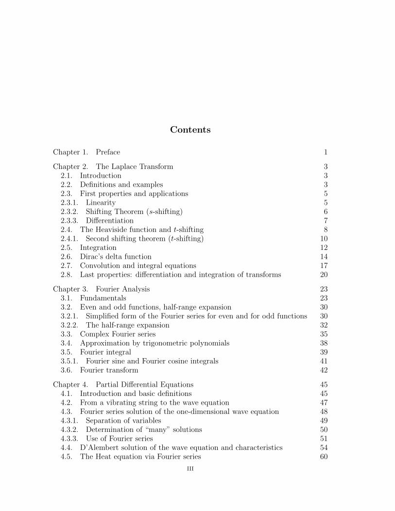
The Laplace transform is one of the most powerful methods in operational calcu-lus, a series of methods that transform differential problems into algebraic problems.
algebraic equations
L
Linv
or
BVP
IVP
Typically these methods are integral transforms of which the Laplace transformand the Fourier transform are examples that we will see.
There are several advantages in using integral transforms in general, and theLaplace transform in particular:
(1) Often algebraic equations are easier to solve;(2) The data of an IVP or a BVP are all encoded in the algebra equation and
the solution is hence found at once without the need of finding the generalsolution and then the particular solution;
(3) It is particularly useful to solve differential equations with input that arenot continuous, for example with short impulses. The way to deal withthese issues is to introduce the Heaviside function and the Dirac delta (see§ 2.6).
2.2. Definitions and examples
Definition 2.1. Let f : [0,∞]→ R be a function. Its Laplace transform is definedas
Lf(s) :=
∫ ∞0
e−stf(t) dt .(2.1)
Notation. (1) There are several ways of denoting the Laplace transform. Amongthe most common are L(f) (and hence L(f)(s) when applied explicitly toa variable s) or F (s).
3
4 2. THE LAPLACE TRANSFORM
(2) It is customary to denote by t the variable for the original function f (e.g.f(t) and g(t)) and by s the variable of the Laplace transform (e.g. L(f)(s)or F (s) and L(g)(s) or G(s)).
Definition 2.2. The function f in (2.1) is the inverse Laplace transform of thefunction F (s) and is often denoted by f := L−1(F ).
Remark 2.3. The inverse Laplace transform is “essentially” uniquely defined, thatis
F1 = F2 ⇒ f1 = f2 .
“Essentially” here means that if two functions (both defined on R≥0 have the sameLaplace transform, then they cannot differ on an interval of positive length, butthey might differ at single points.
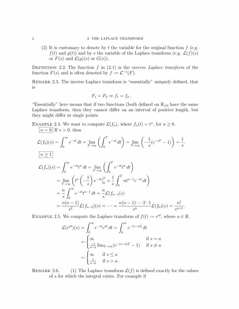
Example 2.4. We want to compute L(fn), where fn(t) = tn, for n ≥ 0.
n = 0 If s > 0, then
L(f0)(s) =
∫ ∞0
e−st dt = limT→∞
(∫ T
0
e−st dt
)= lim
T→∞
(−1
s(e−sT − 1)
)=
1
s.
n ≥ 1
L(fn)(s) =
∫ ∞0
e−sttn dt = limT→∞
(∫ T
0
e−sttn dt
)= lim
T→∞
(tn(−1
s
)e−st
∣∣T0
+1
s
∫ T
0
ntn−1e−st dt
)=n
s
∫ ∞0
e−sttn−1 dt =n
sL(fn−1(s)
=n(n− 1)
s2L(fn−2)(s) = · · · = n(n− 1) · · · 2 · 1
snL(f0)(s) =
n!
sn+1.
Example 2.5. We compute the Laplace transform of f(t) := eat, where a ∈ R.
L(eat)(s) =
∫ ∞0
e−steat dt =
∫ ∞0
e−(s−a)t dt
=
{∞ if s = a−1s−a limT→∞(e−(s−a)T − 1) if s 6= a
=
{∞ if s ≤ a
1s−a if s > a .
Remark 2.6. (1) The Laplace transform L(f) is defined exactly for the valuesof s for which the integral exists. For example if
2.3. FIRST PROPERTIES AND APPLICATIONS 5
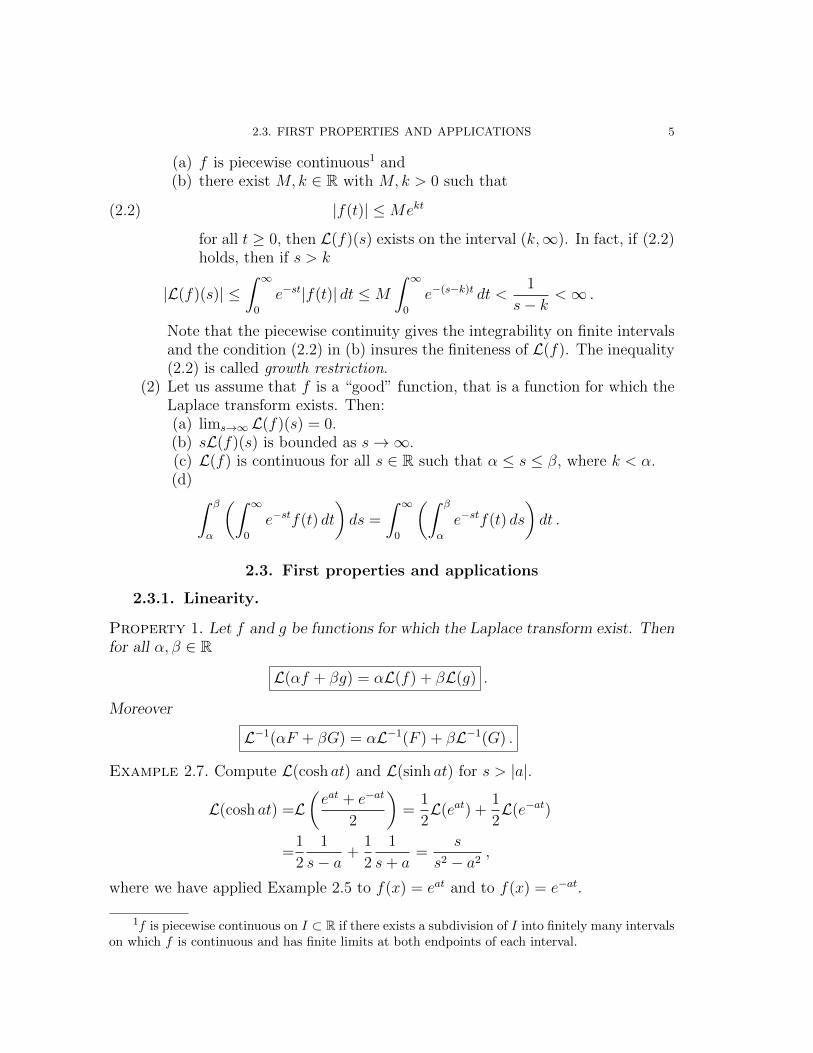
(a) f is piecewise continuous1 and(b) there exist M,k ∈ R with M,k > 0 such that
|f(t)| ≤Mekt(2.2)
for all t ≥ 0, then L(f)(s) exists on the interval (k,∞). In fact, if (2.2)holds, then if s > k
|L(f)(s)| ≤∫ ∞
0
e−st|f(t)| dt ≤M
∫ ∞0
e−(s−k)t dt <1
s− k<∞ .
Note that the piecewise continuity gives the integrability on finite intervalsand the condition (2.2) in (b) insures the finiteness of L(f). The inequality(2.2) is called growth restriction.
(2) Let us assume that f is a “good” function, that is a function for which theLaplace transform exists. Then:(a) lims→∞ L(f)(s) = 0.(b) sL(f)(s) is bounded as s→∞.(c) L(f) is continuous for all s ∈ R such that α ≤ s ≤ β, where k < α.(d) ∫ β
α
(∫ ∞0
e−stf(t) dt
)ds =
∫ ∞0
(∫ β
α
e−stf(t) ds
)dt .
2.3. First properties and applications
2.3.1. Linearity.
Property 1. Let f and g be functions for which the Laplace transform exist. Thenfor all α, β ∈ R
L(αf + βg) = αL(f) + βL(g) .
Moreover
L−1(αF + βG) = αL−1(F ) + βL−1(G) .
Example 2.7. Compute L(cosh at) and L(sinh at) for s > |a|.
L(cosh at) =L(eat + e−at
2
)=
1
2L(eat) +
1
2L(e−at)
=1
2
1
s− a+
1
2
1
s+ a=
s
s2 − a2,
where we have applied Example 2.5 to f(x) = eat and to f(x) = e−at.
1f is piecewise continuous on I ⊂ R if there exists a subdivision of I into finitely many intervalson which f is continuous and has finite limits at both endpoints of each interval.
6 2. THE LAPLACE TRANSFORM
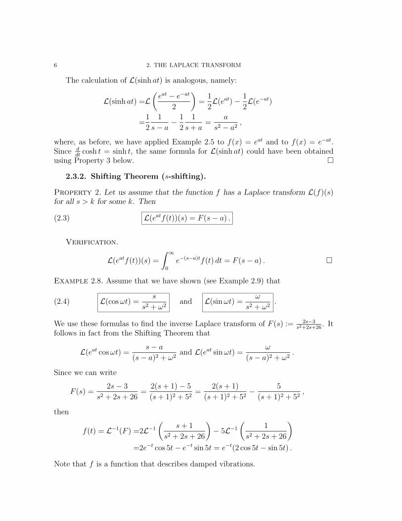
The calculation of L(sinh at) is analogous, namely:
L(sinh at) =L(eat − e−at
2
)=
1
2L(eat)− 1
2L(e−at)
=1
2
1
s− a− 1
2
1
s+ a=
a
s2 − a2,
where, as before, we have applied Example 2.5 to f(x) = eat and to f(x) = e−at.Since d
dtcosh t = sinh t, the same formula for L(sinh at) could have been obtained
using Property 3 below. �
2.3.2. Shifting Theorem (s-shifting).
Property 2. Let us assume that the function f has a Laplace transform L(f)(s)for all s > k for some k. Then
L(eatf(t))(s) = F (s− a) .(2.3)
Verification.
L(eatf(t))(s) =
∫ ∞0
e−(s−a)tf(t) dt = F (s− a) . �
Example 2.8. Assume that we have shown (see Example 2.9) that
L(cosωt) =s
s2 + ω2and L(sinωt) =
ω
s2 + ω2.(2.4)
We use these formulas to find the inverse Laplace transform of F (s) := 2s−3s2+2s+26
. Itfollows in fact from the Shifting Theorem that
L(eat cosωt) =s− a
(s− a)2 + ω2and L(eat sinωt) =
ω
(s− a)2 + ω2.
Since we can write
F (s) =2s− 3
s2 + 2s+ 26=
2(s+ 1)− 5
(s+ 1)2 + 52=
2(s+ 1)
(s+ 1)2 + 52− 5
(s+ 1)2 + 52,
then
f(t) = L−1(F ) =2L−1
(s+ 1
s2 + 2s+ 26
)− 5L−1
(1
s2 + 2s+ 26
)=2e−t cos 5t− e−t sin 5t = e−t(2 cos 5t− sin 5t) .
Note that f is a function that describes damped vibrations.
2.3. FIRST PROPERTIES AND APPLICATIONS 7
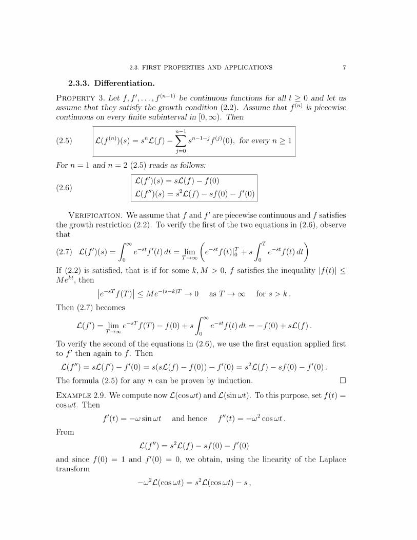
2.3.3. Differentiation.
Property 3. Let f, f ′, . . . , f (n−1) be continuous functions for all t ≥ 0 and let usassume that they satisfy the growth condition (2.2). Assume that f (n) is piecewisecontinuous on every finite subinterval in [0,∞). Then
L(f (n))(s) = snL(f)−n−1∑j=0
sn−1−jf (j)(0), for every n ≥ 1(2.5)
For n = 1 and n = 2 (2.5) reads as follows:
L(f ′)(s) = sL(f)− f(0)
L(f ′′)(s) = s2L(f)− sf(0)− f ′(0)(2.6)
Verification. We assume that f and f ′ are piecewise continuous and f satisfiesthe growth restriction (2.2). To verify the first of the two equations in (2.6), observethat
L(f ′)(s) =
∫ ∞0
e−stf ′(t) dt = limT→∞
(e−stf(t)|T0 + s
∫ T
0
e−stf(t) dt
)(2.7)
If (2.2) is satisfied, that is if for some k,M > 0, f satisfies the inequality |f(t)| ≤Mekt, then ∣∣e−sTf(T )
∣∣ ≤Me−(s−k)T → 0 as T →∞ for s > k .
Then (2.7) becomes
L(f ′) = limT→∞
e−sTf(T )− f(0) + s
∫ ∞0
e−stf(t) dt = −f(0) + sL(f) .
To verify the second of the equations in (2.6), we use the first equation applied firstto f ′ then again to f . Then
L(f ′′) = sL(f ′)− f ′(0) = s(sL(f)− f(0))− f ′(0) = s2L(f)− sf(0)− f ′(0) .
The formula (2.5) for any n can be proven by induction. �
Example 2.9. We compute now L(cosωt) and L(sinωt). To this purpose, set f(t) =cosωt. Then
f ′(t) = −ω sinωt and hence f ′′(t) = −ω2 cosωt .
From
L(f ′′) = s2L(f)− sf(0)− f ′(0)
and since f(0) = 1 and f ′(0) = 0, we obtain, using the linearity of the Laplacetransform
−ω2L(cosωt) = s2L(cosωt)− s ,
8 2. THE LAPLACE TRANSFORM
that is
L(cosωt) =s
s2 + ω2.
The computation of L(sinωt) can be performed analogously. �
Example 2.10 (First application to solving an ODE). We want to find y = y(t)that satisfies the differential equation
y′′ − y = t ,
with initial values
y(0) = 1 and y′(0) = 1 .
Applying the Laplace transform to the equation y′′ − y = t, and using the linearityproperty and Example 2.4, we obtain
L(y′′ − y) = L(t)⇐⇒
s2L(y)− sy(0)− y′(0)− L(y) =1
s2⇐⇒
(s2 − 1)L(y) =1
s2+ s+ 1⇐⇒
L(y) =1
s2 − 1
(1
s2+ s+ 1
).
Using (2.4), Example 2.4, Example 2.5 and Example 2.7, it follows that
L(y) =1
s2(s2 − 1)+
1
s− 1=
1
s2 − 1− 1
s2+
1
s− 1
=L(sinh t)− L(t) + L(et)
=L(sinh t− t+ et) ,
from which we obtain y(t) = sinh t− t+ et.
2.4. The Heaviside function and t-shifting
We want to consider now the vibrations of a mass m on an elastic spring and wedenote by y(t) the displacement. We want to consider the case in which there is adamping force and an external force r(t), so that the differential equation satisfiedby the displacement is
my′′ + cy′ + ky = r(t) ,(2.8)
where c and k are respectively the damping and the spring constants, and wherer(t) is the external force.
The interesting case we want to discuss is when the external force is applied onlyon one interval of time. To do this, we need to introduce the Heaviside function (orunit step function), so defined:
2.4. THE HEAVISIDE FUNCTION AND t-SHIFTING 9
u(t) :=
{1 if t > 0
0 if t < 0 .
0
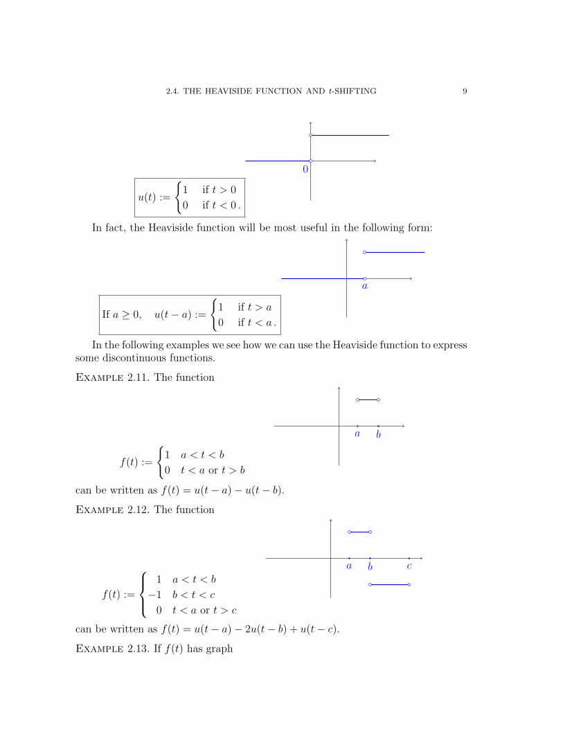
In fact, the Heaviside function will be most useful in the following form:
If a ≥ 0, u(t− a) :=
{1 if t > a
0 if t < a .
a
In the following examples we see how we can use the Heaviside function to expresssome discontinuous functions.
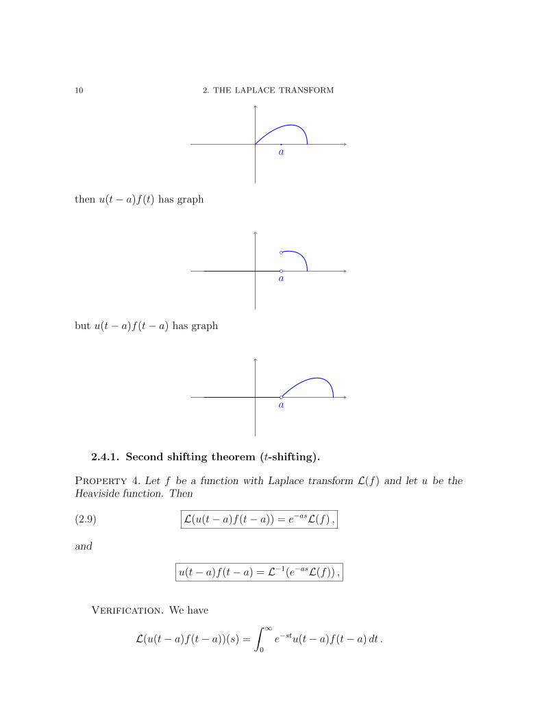
Example 2.11. The function
f(t) :=
{1 a < t < b
0 t < a or t > b
a b
can be written as f(t) = u(t− a)− u(t− b).
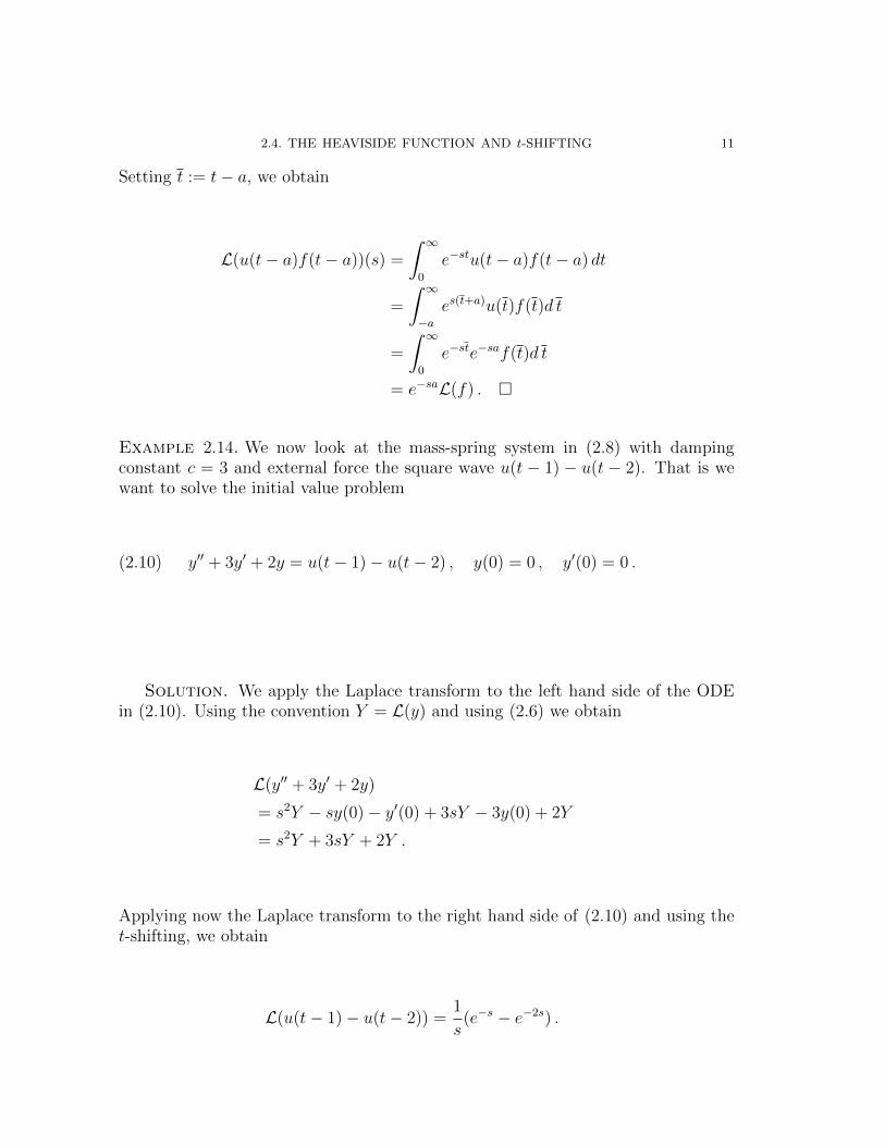
Example 2.12. The function
f(t) :=
1 a < t < b
−1 b < t < c
0 t < a or t > c
a b c
can be written as f(t) = u(t− a)− 2u(t− b) + u(t− c).
Example 2.13. If f(t) has graph
10 2. THE LAPLACE TRANSFORM
a
then u(t− a)f(t) has graph
a
but u(t− a)f(t− a) has graph
a
2.4.1. Second shifting theorem (t-shifting).
Property 4. Let f be a function with Laplace transform L(f) and let u be theHeaviside function. Then
L(u(t− a)f(t− a)) = e−asL(f) ,(2.9)
and
u(t− a)f(t− a) = L−1(e−asL(f)) ,
Verification. We have
L(u(t− a)f(t− a))(s) =
∫ ∞0
e−stu(t− a)f(t− a) dt .
2.4. THE HEAVISIDE FUNCTION AND t-SHIFTING 11
Setting t := t− a, we obtain
L(u(t− a)f(t− a))(s) =
∫ ∞0
e−stu(t− a)f(t− a) dt
=
∫ ∞−a
es(t+a)u(t)f(t)d t
=
∫ ∞0
e−ste−saf(t)d t
= e−saL(f) . �
Example 2.14. We now look at the mass-spring system in (2.8) with dampingconstant c = 3 and external force the square wave u(t − 1) − u(t − 2). That is wewant to solve the initial value problem
y′′ + 3y′ + 2y = u(t− 1)− u(t− 2) , y(0) = 0 , y′(0) = 0 .(2.10)
Solution. We apply the Laplace transform to the left hand side of the ODEin (2.10). Using the convention Y = L(y) and using (2.6) we obtain
L(y′′ + 3y′ + 2y)
= s2Y − sy(0)− y′(0) + 3sY − 3y(0) + 2Y
= s2Y + 3sY + 2Y .
Applying now the Laplace transform to the right hand side of (2.10) and using thet-shifting, we obtain
L(u(t− 1)− u(t− 2)) =1
s(e−s − e−2s) .
12 2. THE LAPLACE TRANSFORM
Setting the two equations above equal to each other, and solving for Y , we obtain,with the help of (2.9) and of Examples 2.4 and 2.5,
Y (s) =1
(s2 + 3s+ 2)s(e−s − e−2s)
=1
s(s+ 1)(s+ 2)(e−s − e−2s)
=
(1
2s− 1
s+ 1+
1
2(s+ 2)
)(e−s − e−2s)
= L(
1
2− e−t +
1
2e−2t
)(e−s − e−2s)
= L(
1
2− e−t +
1
2e−2t
)e−s − L
(1
2− e−t +
1
2e−2t
)e−2s
= L((
1
2− e−(t−1) +
1
2e−2(t−1)
)u(t− 1)
)− L
((1
2− e−(t−2) +
1
2e−2(t−2)
)u(t− 2)
)= L
((1
2− e−(t−1) +
1
2e−2(t−1)
)u(t− 1)−
(1
2− e−(t−2) +
1
2e−2(t−2)
)u(t− 2)
).
It follows that
y(t) =
(1
2− e−(t−1) +
1
2e−2(t−1)
)u(t− 1)−
(1
2− e−(t−2) +
1
2e−2(t−2)
)u(t− 2)
=
0 t < 112− e−(t−1) + 1
2e−2(t−1) 1 < t < 2
e−(t−2) − e−(t−1) + 12e−2(t−1) − 1
2e−2(t−2) t > 2 .
2.5. Integration
Property 5. Let f be a piecewise continuous function for t ≥ 0 that satisfies thegrowth condition (2.2). Then for s > k, s > 0, and t > 0
L(∫ t
0
f(x) dx
)=
1
sF (s) .(2.11)
and ∫ t
0
f(x) dx = L−1
(1
sF (s)
).(2.12)
Verification. Let g(t) :=∫ t
0f(x) dx and let us verify first that if f satisfies
the growth condition, so does g. In fact,
|g(t)| ≤∫ t
0
|f(x)| dx ≤M
∫ t
0
ekx dx =M
k(ekt − 1) ≤ M
kekt .
2.5. INTEGRATION 13
Moreover g′(t) = f(t) and g(0) = 0, hence from (2.6) we have
L(g′) = sL(g)− g(0) = sL(g) ,
which implies that
L(∫ t
0
f(x) dx
)= L(g(t)) =
1
sL(g′) =
1
sL(f) . �
Example 2.15. Compute L−1(
1s(s2+ω2)
)and L−1
(1
s2(s2+ω2)
).
Solution. We know that L(sinωt) = ωs2+ω2 . Since ω is a constant, by linearity
of the Laplace transform we obtain
L(
sinωt
ω
)=
1
s2 + ω2,
and multiplying by 1s
1
sL(
sinωt
ω
)=
1
s
(1
s2 + ω2
).
Taking the inverse Laplace transform on both sides, and using (2.12), we obtain
L−1
(1
s
(1
s2 + ω2
))= L−1
(1
sL(
sinωt
ω
))=
∫ t
0
sinωx
ωdx
=1
ω2(− cosωx)|t0
=1
ω2(1− cosωt) .
To compute L−1(
1s2(s2+ω2)
)we iterate the above calculation. We know that
L(
1
ω2(1− cosωt)
)=
1
ω2
(1
s− s
s2 + ω2
)=
1
s(s2 + ω2),
from which it follows, again using (2.12), that
L−1
(1
s2(s2 + ω2)
)= L−1
(1
sL(
1
ω2(1− cosωt)
))=
1
ω2
∫ t
0
(1− cosωx) dx
=1
ω2
(t− 1
ωsinωt
).
14 2. THE LAPLACE TRANSFORM
Example 2.16 ([?, Example 6, page 232]). Solve
y′′ + y = 2t , y(π
4
)= π/2 , y′
(π4
)= 2−
√2 .(2.13)
Solution. We set t := t − π/4, from which t = t + π/4. With respect to thisnew variable we have
y(t) = y(t) , y′(t) = y′(t) , y′′(t) = y′′(t) ,
and hence (2.13) becomes
y′′ + y = 2(t+
π
4
), y(0) =
π
2, y′(0) = 2−
√2 .
Applying the Laplace transform to the ODE we obtain
s2L(y)− sy(0)− y′(0) + L(y) = 2L(t) +π
2L(1) ,
from which it follows that
(s2 + 1)Y − π
2s− 2 +
√2 =
2
s2+π
2s.
Solving for Y , and using the result of both computations in Example 2.15, we obtain
Y =2
s2(s2 + 1)+π
2
1
s(s2 + 1)+
2−√
2
s2 + 1+π
2
s
s2 + 1
= 2L(t− sin t) +π
2L(1− cos t) + (2−
√2)L(sin t) +
π
2L(cos t)
= L(2t+π
2−√
2 sin t) .
Hence
y(t) = 2t+π
2−√
2 sin t ,
and substituting back to obtain the original variable t we obtain
y(t) = 2(t− π
4
)+π
2−√
2 sin(t− π
4
)= 2t−
√2
1√2
(sin t− cos t)
= 2t− sin t+ cos t .
2.6. Dirac’s delta function
We are going to look for solutions of the differential equationmy′′+cy′+ky = r(t),where r(t) is a force over a very short interval of time, almost instantaneously.Phenomena of this impulsive nature are common and can be dealt with using Dirac’sdelta.
2.6. DIRAC’S DELTA FUNCTION 15
We saw already how to deal with forces applied on an interval [a, a+ h] and weassume now that the magnitude of the force is 1/h, so that the impulse of the forceis one. Namely if
fh(t− a) :=
{1/h a ≤ t ≤ a+ h
0 otherwise ,
then
Ih :=
∫ ∞0
fh(t− a) dt =
∫ a+h
a
1
hdt = 1 .
Definition 2.17. The Dirac delta is the limit
δ(t− a) := limh→0
fh(t) =
{∞ t = a
0 t 6= a ,
and
∫ ∞0
δ(t− a) dt = 1 .(2.14)
Remark 2.18. The Dirac delta function is not a function, but a generalised functionor a distribution.
The following properties are important and should be shown using the definitionof distribution:
Property 6. (1) (Sifting property)
∫ ∞0
g(t)δ(t− a) dt = g(a) ,(2.15)
(2) L(δ(t− a)) = e−as .
Verification. (1) This is consistent with (2.14) in the case in which g(t) ≡ 1.
16 2. THE LAPLACE TRANSFORM
(2) We use here properties of the Dirac delta and of the Laplace transform. Becausethe Laplace transform has good convergence properties, we can write
L(δ(t− a)) = L(limh→0
fh(t− a))
= limh→0L(fh(t− a))
= limh→0
1
hL(u(t− a)− u(t− (a+ h)))
= limh→0
1
hs(e−as − e−(a+h)s)
= limh→0
e−as1− e−hs
hs
= e−as limh→0
1− e−hs
hs
(∗)= e−as lim
h→0
se−hs
s= e−as ,
where in (∗) we used either the fact that
limh→0
1− e−hs
hs= lim
hs→0
1− e−hs
hs= lim
`→0
1− e−`
`= − d
d`e−`∣∣∣∣`=0
= e−`|`=0 = 1 .
or l’Hopital rule.Another possibility would have been to apply (2.15) with g(t) = e−at. Having
done the direct calculation provides instead further evidence for (2.15). �
Example 2.19. (Hammerblow response of a mass-spring system) We want to solvethe IVP
y′′ + 3y′ + 2y = δ(t− 1) , y(0) = 0 , y′(0) = 0 .
Solution. We apply the Laplace transform to both sides of the ODE
L(y′′ + 3y′ + 2y) = L(δ(t− 1))
and, using the calculation in Example 2.14 we obtain that
s2Y + 3sY + 2Y = e−s ,
or, equivalently,
Y =1
(s+ 1)(s+ 2)e−s =
(1
s+ 1− 1
s+ 2
)e−s .(2.16)
We apply now the second Shifting theorem (Property 4) with L(e−at) = 1s+a
anda = 1, 2, that is
1s+1
e−s = L(e−t)e−s = L(u(t− 1)e−(t−1))(2.17)
1s+2
e−s = L(e−2t)e−s = L(u(t− 1)e−2(t−1)) .(2.18)
2.7. CONVOLUTION AND INTEGRAL EQUATIONS 17
Plugging in the result of the two equations in (2.17) into (2.16) we obtain
Y = L(u(t− 1)(e−(t−1) − e−2(t−1))) ,
that is
y = u(t− 1)(e−(t−1) − e−2(t−1))
�
2.7. Convolution and integral equations
While the Laplace transform is linear and satisfies the property L(f+g) = L(f)+L(g), the same cannot be said about the product of two functions. In other wordsL(f ·g) 6= L(f)L(g). However one can define a different “product”, called convolutionand denoted by ∗, that has the desired property that L(f ∗ g) = L(f)L(g).
Definition 2.20. The convolution f ∗ g of two functions f and g is defined as
f ∗ g(t) :=
∫ t
0
f(t′)g(t− t′) dt′ .
Properties. Let f, g and h be functions. Then:
(1) f ∗ g = g ∗ f ;(2) f ∗ (g + h) = f ∗ g + f ∗ h;(3) f ∗ (g ∗ h) = (f ∗ g) ∗ h;(4) f ∗ 0 = 0 ∗ f = 0;(5) f ∗ 1 6= f ;(6) f ∗ f is not always non-negative.
The verification of these properties is straightforward and is similar to the ver-ification of the Property 7 that we will do later. An example that illustrates (5)is f(t) = t, since f ∗ 1 = 1
2t2. On the other hand, taking f(t) = sin t, shows that
f ∗ f = 12
cos t+ 12
sin t can take also negative values.
Property 7. If f, g are two functions, then
L(f ∗ g) = L(f)L(g) .
Verification. By definition we have
L(f ∗ g)(s) =
∫ ∞0
e−st(f ∗ g)(t) dt
=
∫ ∞0
e−st(∫ t
0
f(t′)g(t− t′) dt′)dt
(2.19)
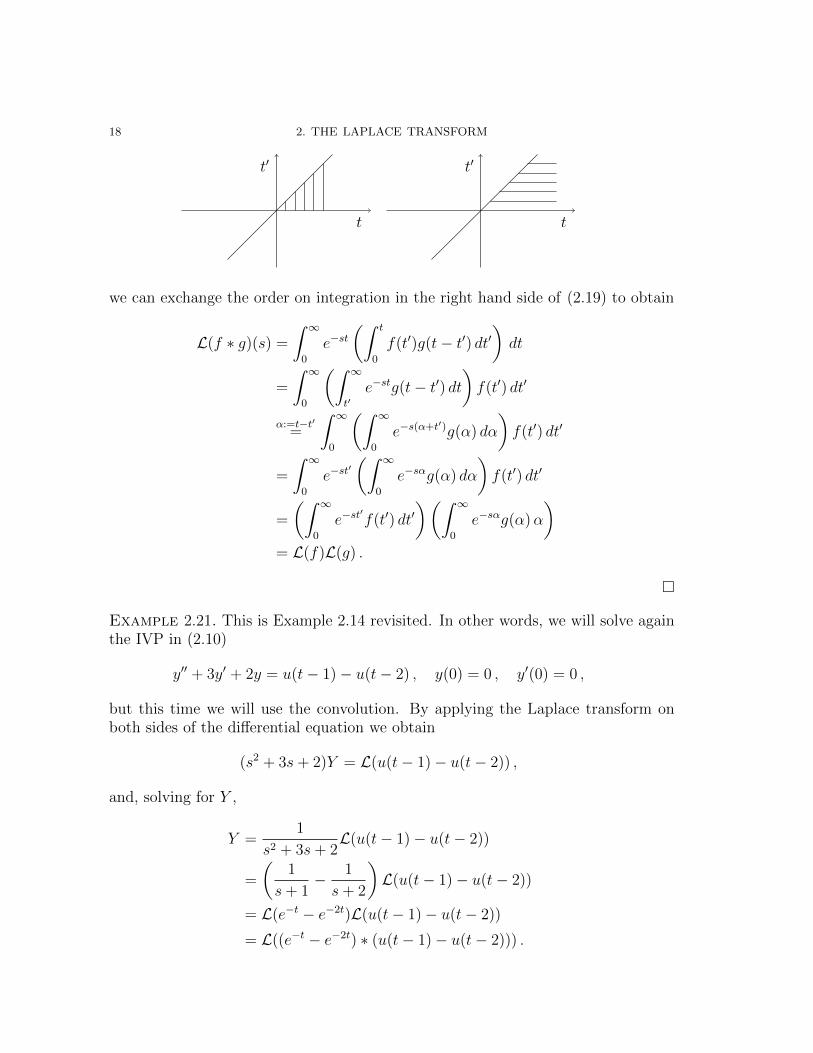
Since
{(t, t′) : 0 < t′ < t, 0 < t <∞} = {(t, t′) : t′ < t <∞, 0 < t′ <∞} ,
18 2. THE LAPLACE TRANSFORM
t
t′
t
t′
we can exchange the order on integration in the right hand side of (2.19) to obtain
L(f ∗ g)(s) =
∫ ∞0
e−st(∫ t
0
f(t′)g(t− t′) dt′)dt
=
∫ ∞0
(∫ ∞t′
e−stg(t− t′) dt)f(t′) dt′
α:=t−t′=
∫ ∞0
(∫ ∞0
e−s(α+t′)g(α) dα
)f(t′) dt′
=
∫ ∞0
e−st′(∫ ∞
0
e−sαg(α) dα
)f(t′) dt′
=
(∫ ∞0
e−st′f(t′) dt′
)(∫ ∞0
e−sαg(α)α
)= L(f)L(g) .
�
Example 2.21. This is Example 2.14 revisited. In other words, we will solve againthe IVP in (2.10)
y′′ + 3y′ + 2y = u(t− 1)− u(t− 2) , y(0) = 0 , y′(0) = 0 ,
but this time we will use the convolution. By applying the Laplace transform onboth sides of the differential equation we obtain
(s2 + 3s+ 2)Y = L(u(t− 1)− u(t− 2)) ,
and, solving for Y ,
Y =1
s2 + 3s+ 2L(u(t− 1)− u(t− 2))
=
(1
s+ 1− 1
s+ 2
)L(u(t− 1)− u(t− 2))
= L(e−t − e−2t)L(u(t− 1)− u(t− 2))
= L((e−t − e−2t) ∗ (u(t− 1)− u(t− 2))) .
2.7. CONVOLUTION AND INTEGRAL EQUATIONS 19
It follows that
y(t) = (e−t − e−2t) ∗ (u(t− 1)− u(t− 2))
= (u(t− 1)− u(t− 2)) ∗ (e−t − e−2t)
=
∫ t
0
(u(t′ − 1)− u(t′ − 2))(e−(t−t′) − e−2(t−t′)) dt′(2.20)
Since ∫e−a(t−t′) dt′ =
1
ae−a(t−t′) + C ,
then ∫(e−(t−t′) − e−2(t−t′)) dt′ = e−(t−t′) − 1
2e−2(t−t′) + C .
If follows from (2.20) that, if 1 < t < 2,
y(t) =
∫ t
1
(u(t′ − 1)− u(t′ − 2))(e−(t−t′) − e−2(t−t′)) dt′
=
∫ t
1
(e−(t−t′) − e−2(t−t′)) dt′
= (e−(t−t′) − 1
2e−2(t−t′))
∣∣t1
=1
2− e−(t−1) +
1
2e−2(t−1) .
On the other hand, if t > 2, (2.20) becomes
y(t) =
∫ 2
1
(u(t′ − 1)− u(t′ − 2))(e−(t−t′) − e−2(t−t′)) dt′
=
∫ 2
1
(e−(t−t′) − e−2(t−t′)) dt′
= (e−(t−t′) − 1
2e−2(t−t′))
∣∣21
= e−(t−2) − 1
2e−2(t−2) − e−(t−1) +
1
2e−2(t−1) ,
which is consistent with the result obtained in Exercise 2.14.
Example 2.22. Solve the integral equation
y(t)−∫ t
0
y(t′) sin(t− t′) dt′ = t .
Solution. Since∫ t
0y(t′) sin(t− t′) = y(t) ∗ sin t, by applying the Laplace trans-
form to the equation
y − y ∗ sin t = t
20 2. THE LAPLACE TRANSFORM
we obtain
Y − Y 1
s2 + 1=
1
s2.
Solving for Y we get
Y =s2 + 1
s4=
1
s2+
1
s4= L
(t+
1
6t3),
from which we gather that y(t) = t+ 16t3. �
2.8. Last properties: differentiation and integration of transforms
We saw already how the Laplace transform of the derivative or of the integralof a function is related to the Laplace transform of the function (Properties 3 and4). Here we see the effect of taking the derivative or the integral of the Laplacetransform.
Property 8. Let f be a piecewise continuous function that satisfies the growthcondition (2.2). Then
(1) L′(f) = −L(tf(t)).
(2) If in addition limt→0+f(t)t
exists, then∫∞sL(f)(s′) ds′ = L
(f(t)t
).
Verification. (1) The continuity properties of the Laplace transform allow usto write
d
ds
∫ ∞0
e−stf(t) dt =
∫ ∞0
−te−stf(t) dt .
The right hand side of the above equality equals −L(tf(t)), from which the firstassertion follows.
(2) The same continuity properties of the Laplace transform used in (1) allow us towrite ∫ ∞
s
(∫ ∞0
e−ts′f(t) dt
)ds′ =
∫ ∞0
(∫ ∞s
e−ts′ds′)f(t) dt .(2.21)
The right hand side of (2.21) equals∫ ∞0
(−1
te−ts
′∣∣∣∣∞s
)f(t) dt =
∫ ∞0
e−st1
tf(t) dt = L
(1
tf(t)
),
which shows the second assertion. �
Remark 2.23. Let f : R→ R be a function that is piecewise continuous, satisfies thegrowth condition (2.2) with constants M and k and has the property that f(t) = 0if t < 0. Then the Laplace transform of f exists for all complex numbers z ∈ C withreal part <z > k. Considering the Laplace transform as a function of a complexvariable has for example the advantage that there exists a formula for the inverse
2.8. LAST PROPERTIES: DIFFERENTIATION AND INTEGRATION OF TRANSFORMS 21
Laplace transform. However the knowledge needed to use this formula is beyondthe scope of this course and is therefore not treated here.

CHAPTER 3
Fourier Analysis
Fourier series are an instrument to decompose periodic phenomena, such as thebehaviour of a rotating part in a machine, into simpler functions such as sinesand cosines. We will see that Fourier integrals give a way of extending a similardecomposition to the case of non-periodic phenomena.
3.1. Fundamentals
Definition 3.1. A function f(x) is called periodic if it is defined for “most” x ∈ Rand if there is a positive real number p ∈ R, p > 0 such that f(x) = f(x+ p) for allx.
Example 3.2. f(x) = sinx and f(x) = cos x are periodic of period p = 2π.
Remark 3.3. The period p is not necessarily the smallest real number for whichf(x) = f(x + p). In fact, if p is a period, then any multiple of p is also a period.This is important in the following examples:
Example 3.4. (1) f(x) = sinnx and f(x) = cosnx are periodic of period 2π/nbut also periodic of period p = 2π: we will consider them as periodic ofperiod 2π.
(2) sin(nπLx)
and cos(nπLx)
are periodic of period 2L/n but we will considerthem in the following as functions of period 2L.
(3) f(x) = tanx is periodic of period π. This is the typical example of afunction that is defined for “most” x, as it is defined for all x 6= ±(2k+1)π
2,
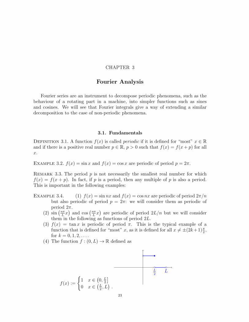
for k = 0, 1, 2, . . . .(4) The function f : (0, L)→ R defined as
f(x) :=
{1 x ∈
(0, L
2
]0 x ∈
(L2, L).
L2
L
23
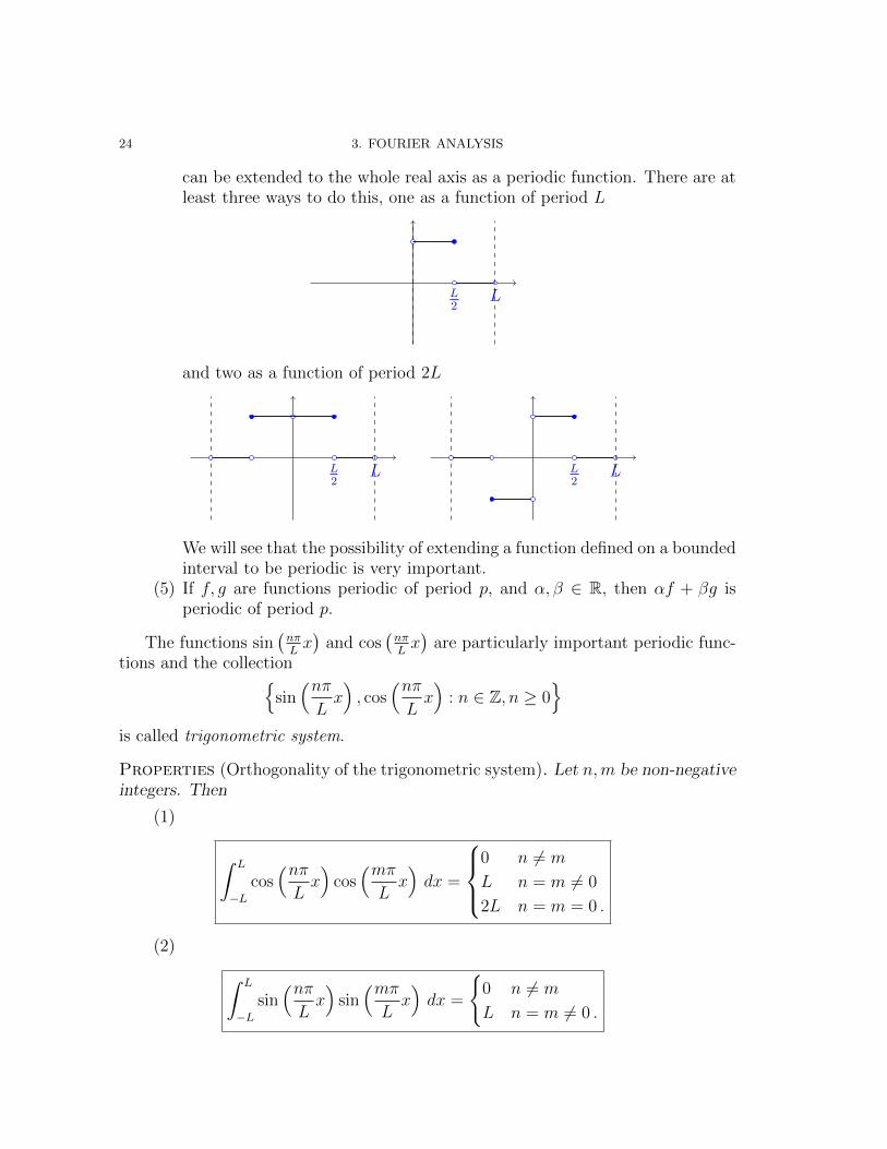
24 3. FOURIER ANALYSIS
can be extended to the whole real axis as a periodic function. There are atleast three ways to do this, one as a function of period L
L2
L
and two as a function of period 2L
L2
L L2
L
We will see that the possibility of extending a function defined on a boundedinterval to be periodic is very important.
(5) If f, g are functions periodic of period p, and α, β ∈ R, then αf + βg isperiodic of period p.
The functions sin(nπLx)
and cos(nπLx)
are particularly important periodic func-tions and the collection{
sin(nπLx), cos
(nπLx)
: n ∈ Z, n ≥ 0}
is called trigonometric system.
Properties (Orthogonality of the trigonometric system). Let n,m be non-negativeintegers. Then
(1)
∫ L
−Lcos(nπLx)
cos(mπLx)dx =
0 n 6= m
L n = m 6= 0
2L n = m = 0 .
(2) ∫ L
−Lsin(nπLx)
sin(mπLx)dx =
{0 n 6= m
L n = m 6= 0 .
3.1. FUNDAMENTALS 25
(3) ∫ L
−Lcos(nπLx)
sin(mπLx)dx = 0, for every n,m .
Verification. To simplify the calculation we consider the case in which 2L =2π. Observe first of all that if n = m = 0, then∫ π
−πcosnx cosmxdx =
∫ π
−πdx = 2π .
Using the following trigonometric formulas
cosnx cosmx =1
2cos(n+m)x+
1
2cos(n−m)x
sinnx sinmx =1
2cos(n−m)x− 1
2cos(n+m)x
sinnx cosmx =1
2sin(n+m)x+
1
2sin(n−m)x ,
we obtain∫ π
−πcosnx cosmxdx =
1
2
∫ π
−πcos(n+m)x dx+
1
2
∫ π
−πcos(n−m)x dx
=
{120 + 1
20 = 0 n 6= m
π n = m 6= 0,
∫ π
−πsinnx sinmxdx =
1
2
∫ π
−πcos(n−m)x dx+
1
2
∫ π
−πcos(n+m)x dx
=
{120 + 1
20 = 0 n 6= m
π n = m 6= 0,
and finally∫ π
−πcosnx sinmxdx =
1
2
∫ π
−πsin(n+m)x dx+
1
2
∫ π
−πsin(n−m)x dx
=1
20 +
1
20 = 0 .
�
Definition 3.5. (1) A trigonometric polynomial is a function of the kind
a0 +N∑n=1
(an cos
(nπLx)
+ bn sin(nπLx))
,
while
26 3. FOURIER ANALYSIS
(2) a trigonometric series is a function of the kind
a0 +∞∑n=1
(an cos
(nπLx)
+ bn sin(nπLx))
,
where the an, bn are constants called the coefficients.
Since the functions in the trigonometric system are periodic of period 2L andsince a trigonometric series is the sum of functions in the trigonometric system, ifthe series converges it will converge to a periodic function of period 2L. Supposethis is the case and let f(x) be a function whose sum is a trigonometric series, thatis
f(x) = a0 +∞∑n=1
(an cos
(nπLx)
+ bn sin(nπLx))
.(3.1)
The natural question is what is the relation between f(x) and the coefficients an, bn.By multiplying both sides of (3.1) by cos
(mπLx)
and integrating the result over theinterval [−L,L], we obtain∫ L
−Lf(x) cos
(mπLx)dx
= a0
∫ L
−Lcos(mπLx)dx+
∞∑n=1
(an
∫ L
−Lcos(nπLx)
cos(mπLx)dx
+ bn
∫ L
−Lsin(nπLx)
cos(mπLx)dx︸ ︷︷ ︸
=0
).
Using the orthogonality properties of the trigonometric system (in particular (1)and (3) for m fixed and n varying between 1 and ∞) we obtain∫ L
−Lf(x) cos
(mπLx)dx =
{a02L m = 0
amL m > 0 ,
from which it follows that
a0 =1
2L
∫ L
−Lf(x) dx ,
am =1
L
∫ L
−Lf(x) cos
(mπLx)dx , if m > 0 .
(3.2)
3.1. FUNDAMENTALS 27
Likewise, multiplying both sides of (3.1) by sin(mπLx)
and integrating the resultover the interval [−L,L], we obtain
∫ L
−Lf(x) sin
(mπLx)dx
= a0
∫ L
−Lsin(mπLx)dx︸ ︷︷ ︸
=0
+∞∑n=1
(an
∫ L
−Lcos(nπLx)
sin(mπLx)dx︸ ︷︷ ︸
=0
+ bn
∫ L
−Lsin(nπLx)
sin(mπLx)dx
).
Again using the orthogonality properties of the trigonometric system we deduce
bm =1
L
∫ L
−Lf(x) sin
(mπLx)dx , if m > 0 .(3.3)
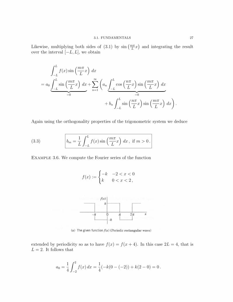
Example 3.6. We compute the Fourier series of the function
f(x) :=
{−k −2 < x < 0
k 0 < x < 2 ,
extended by periodicity so as to have f(x) = f(x + 4). In this case 2L = 4, that isL = 2. It follows that
a0 =1
4
∫ 2
−2
f(x) dx =1
4(−k(0− (−2)) + k(2− 0) = 0 .
28 3. FOURIER ANALYSIS
and
am =1
L
∫ L
−Lf(x) cos
(mπLx)dx
=k
2
(−∫ 0
−2
cos(mπ
2x)dx+
∫ 2
0
cos(mπ
2x))
dx
=k
�2
�2
mπ
(− sin
(mπ2x) ∣∣0−2
+ sin(mπ
2x) ∣∣2
0
)=
k
mπ
(sin(mπ�2
(−�2))
+ sin(mπ�2�2))
= 0 .
Analogously
bm =1
L
∫ L
−Lf(x) sin
(mπLx)dx
=k
2
(−∫ 0
−2
sin(mπ
2x)dx+
∫ 2
0
sin(mπ
2x))
dx
=k
�2
�2
mπ
(cos(mπ
2x) ∣∣0−2− cos
(mπ2x) ∣∣2
0
)=
k
mπ(1− cos(−mπ)− cos(mπ) + 1)
=2k
mπ(1− cosmπ)
=
{4kmπ
m = 1, 3, 5, . . .
0 m = 2, 4, 6, . . . .
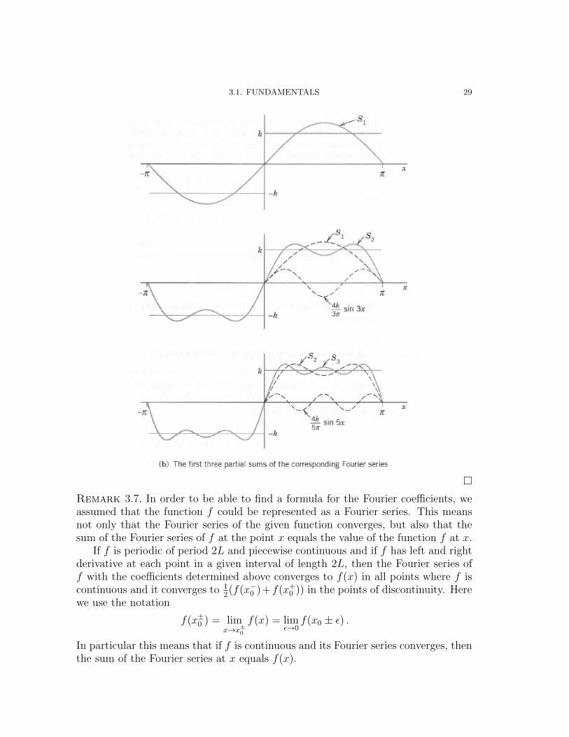
Thus f(x) can be represented by a Fourier series as follows
f(x) =4k
π
∞∑n=0
1
2n+ 1sin
((2n+ 1)π
2x
).
3.1. FUNDAMENTALS 29
�
Remark 3.7. In order to be able to find a formula for the Fourier coefficients, weassumed that the function f could be represented as a Fourier series. This meansnot only that the Fourier series of the given function converges, but also that thesum of the Fourier series of f at the point x equals the value of the function f at x.
If f is periodic of period 2L and piecewise continuous and if f has left and rightderivative at each point in a given interval of length 2L, then the Fourier series off with the coefficients determined above converges to f(x) in all points where f iscontinuous and it converges to 1
2(f(x−0 )+f(x+
0 )) in the points of discontinuity. Herewe use the notation
f(x±0 ) = limx→x±0
f(x) = limε→0
f(x0 ± ε) .
In particular this means that if f is continuous and its Fourier series converges, thenthe sum of the Fourier series at x equals f(x).
30 3. FOURIER ANALYSIS
3.2. Even and odd functions, half-range expansion
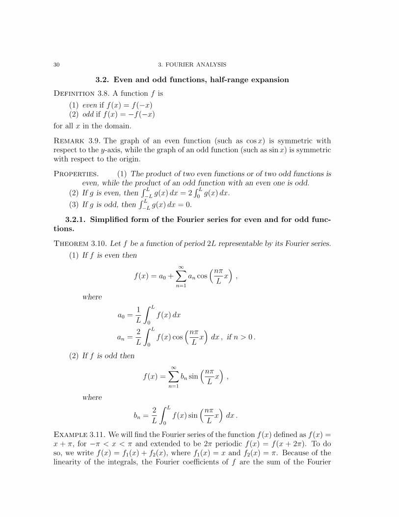
Definition 3.8. A function f is
(1) even if f(x) = f(−x)(2) odd if f(x) = −f(−x)
for all x in the domain.
Remark 3.9. The graph of an even function (such as cos x) is symmetric withrespect to the y-axis, while the graph of an odd function (such as sinx) is symmetricwith respect to the origin.
Properties. (1) The product of two even functions or of two odd functions iseven, while the product of an odd function with an even one is odd.
(2) If g is even, then∫ L−L g(x) dx = 2
∫ L0g(x) dx.
(3) If g is odd, then∫ L−L g(x) dx = 0.
3.2.1. Simplified form of the Fourier series for even and for odd func-tions.
Theorem 3.10. Let f be a function of period 2L representable by its Fourier series.
(1) If f is even then
f(x) = a0 +∞∑n=1
an cos(nπLx),
where
a0 =1
L
∫ L
0
f(x) dx
an =2
L
∫ L
0
f(x) cos(nπLx)dx , if n > 0 .
(2) If f is odd then
f(x) =∞∑n=1
bn sin(nπLx),
where
bn =2
L
∫ L
0
f(x) sin(nπLx)dx .
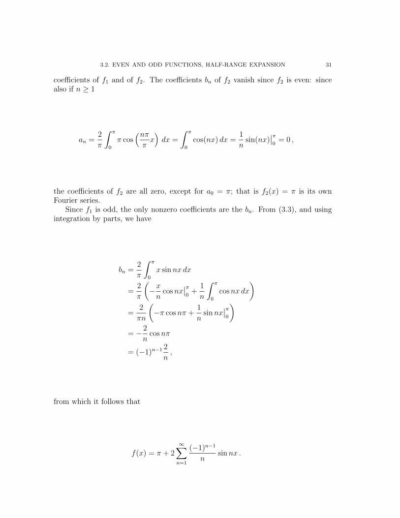
Example 3.11. We will find the Fourier series of the function f(x) defined as f(x) =x + π, for −π < x < π and extended to be 2π periodic f(x) = f(x + 2π). To doso, we write f(x) = f1(x) + f2(x), where f1(x) = x and f2(x) = π. Because of thelinearity of the integrals, the Fourier coefficients of f are the sum of the Fourier
3.2. EVEN AND ODD FUNCTIONS, HALF-RANGE EXPANSION 31
coefficients of f1 and of f2. The coefficients bn of f2 vanish since f2 is even: sincealso if n ≥ 1
an =2
π
∫ π
0
π cos(nππx)dx =
∫ π
0
cos(nx) dx =1
nsin(nx)
∣∣π0
= 0 ,
the coefficients of f2 are all zero, except for a0 = π; that is f2(x) = π is its ownFourier series.
Since f1 is odd, the only nonzero coefficients are the bn. From (3.3), and usingintegration by parts, we have
bn =2
π
∫ π
0
x sinnx dx
=2
π
(−xn
cosnx∣∣π0
+1
n
∫ π
0
cosnx dx
)=
2
πn
(−π cosnπ +
1
nsinnx
∣∣π0
)= − 2
ncosnπ
= (−1)n−1 2
n,
from which it follows that
f(x) = π + 2∞∑n=1
(−1)n−1
nsinnx .
32 3. FOURIER ANALYSIS
3.2.2. The half-range expansion. We saw in Example 3.4(4) that a functionf defined on the interval (0, L) can be extended periodically with period L and inthis case its Fourier series will contain both coefficients an and bn. Sometimes it ishowever convenient to extend the function f to be either even or odd, and in thiscase the period will be 2L. This is particularly convenient in connection with PDEs,as we will see in Chapter 4.
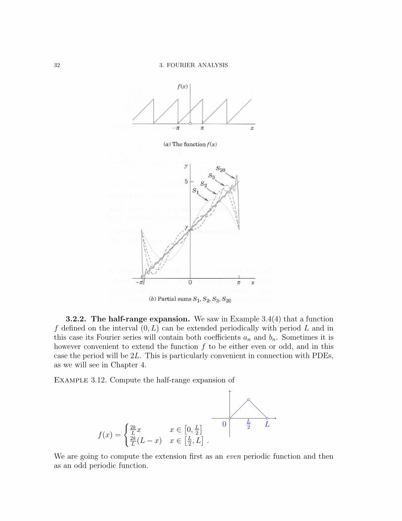
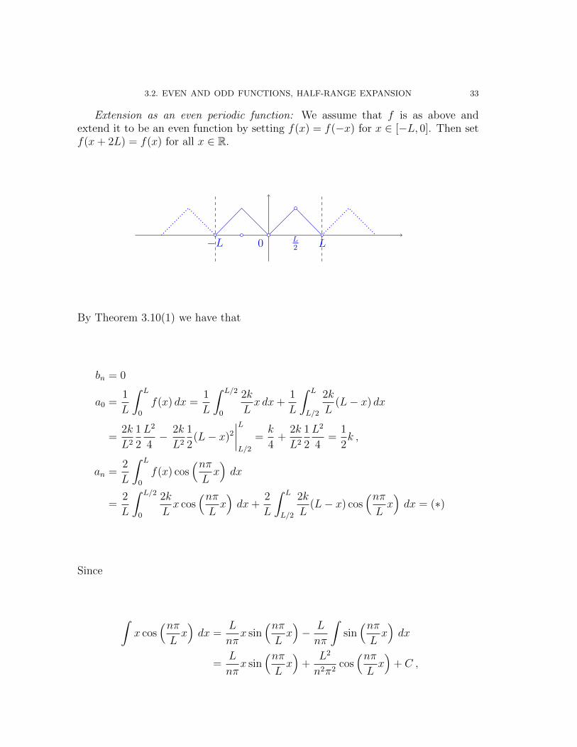
Example 3.12. Compute the half-range expansion of
f(x) =
{2kLx x ∈
[0, L
2
]2kL
(L− x) x ∈[L2, L].
0 L2 L
We are going to compute the extension first as an even periodic function and thenas an odd periodic function.
3.2. EVEN AND ODD FUNCTIONS, HALF-RANGE EXPANSION 33
Extension as an even periodic function: We assume that f is as above andextend it to be an even function by setting f(x) = f(−x) for x ∈ [−L, 0]. Then setf(x+ 2L) = f(x) for all x ∈ R.
−L 0 L2 L
By Theorem 3.10(1) we have that
bn = 0
a0 =1
L
∫ L
0
f(x) dx =1
L
∫ L/2
0
2k
Lx dx+
1
L
∫ L
L/2
2k
L(L− x) dx
=2k
L2
1
2
L2
4− 2k
L2
1
2(L− x)2
∣∣∣∣LL/2
=k
4+
2k
L2
1
2
L2
4=
1
2k ,
an =2
L
∫ L
0
f(x) cos(nπLx)dx
=2
L
∫ L/2
0
2k
Lx cos
(nπLx)dx+
2
L
∫ L
L/2
2k
L(L− x) cos
(nπLx)dx = (∗)
Since
∫x cos
(nπLx)dx =
L
nπx sin
(nπLx)− L
nπ
∫sin(nπLx)dx
=L
nπx sin
(nπLx)
+L2
n2π2cos(nπLx)
+ C ,
34 3. FOURIER ANALYSIS
then
(∗) =4k
L2
(L
nπx sin
(nπLx)
+L2
n2π2cos(nπLx))∣∣∣∣L/2
0
+4k
L
∫ L
L/2
cos(nπLx)dx
−4k
L2
(L
nπx sin
(nπLx)
+L2
n2π2cos(nπLx))∣∣∣∣L
L/2
=2k
nπsin(nπ
2
)+
4k
n2π2cos(nπ
2
)− 4k
n2π2
+4k
nπsinnπ − 4k
nπsin(nπ
2
)−4k
L2
(L2
nπsinnπ − L2
2nπsin(nπ
2
))+
L2
n2π2
(cosnπ − cos
(nπ
2
))=
(2k
nπ− 4k
nπ+
2k
nπ
)︸ ︷︷ ︸
=0
sin(nπ
2
)+
(4k
n2π2+
4k
n2π2
)︸ ︷︷ ︸
= 8kn2π2
cos(nπ
2
)
+
(4k
nπ− 4k
nπ
)︸ ︷︷ ︸
=0
sinnπ − 4k
n2π2cosnπ− 4k
n2π2
=8k
n2π2cos(nπ
2
)− 4k
n2π2cosnπ − 4k
n2π2
=4k
n2π2
(2 cos
(nπ
2
)− cosnπ − 1
).
Since cosnπ = (−1)n and cos(nπ
2
)=
{0 n = 2j + 1
(−1)j n = 2j, then
an =(
2 cos(nπ
2
)− cosnπ − 1
)=
{4kn2π2
(2 · 0− (−1)2j+1 − 1
)n = 2j + 1
4kn2π2
(2(−1)j − (−1)2j − 1
)n = 2j
=
{4kn2π2
((−1)2j − 1
)n = 2j + 1
4kn2π2
(2(−1)j − 2
)n = 2j
=
0 n = 2j + 1
0 n = 2j,with j even, that is j = 2m4kn2π2 (−4) = − 16k
n2π2 n = 2j,with j odd, that is j = 2m+ 1 ,
3.3. COMPLEX FOURIER SERIES 35
so that
f(x) =k
2− 16k
π2
(1
22cos
(2π
Lx
)+
1
62cos
(6π
Lx
)+ . . .
)=k
2− 16k
π2
∞∑m=0
1
(2(2m+ 1))2cos
(2(2m+ 1)
Lx
).
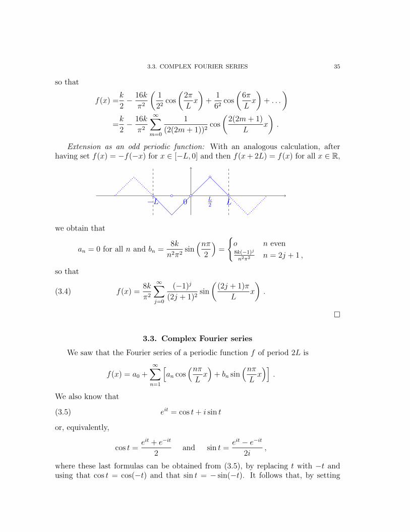
Extension as an odd periodic function: With an analogous calculation, afterhaving set f(x) = −f(−x) for x ∈ [−L, 0] and then f(x+ 2L) = f(x) for all x ∈ R,
−L 0 L2 L
we obtain that
an = 0 for all n and bn =8k
n2π2sin(nπ
2
)=
{o n even8k(−1)j
n2π2 n = 2j + 1 ,
so that
f(x) =8k
π2
∞∑j=0
(−1)j
(2j + 1)2sin
((2j + 1)π
Lx
).(3.4)
�
3.3. Complex Fourier series
We saw that the Fourier series of a periodic function f of period 2L is
f(x) = a0 +∞∑n=1
[an cos
(nπLx)
+ bn sin(nπLx)]
.
We also know that
eit = cos t+ i sin t(3.5)
or, equivalently,
cos t =eit + e−it
2and sin t =
eit − e−it
2i,
where these last formulas can be obtained from (3.5), by replacing t with −t andusing that cos t = cos(−t) and that sin t = − sin(−t). It follows that, by setting
36 3. FOURIER ANALYSIS
nπLx =: tn for n > 0 for simplicity,
an cos tn + bn sin tn = aneitn + e−itn
2+ bn
eitn − e−itn2i
= eitn1
2(an − ibn)︸ ︷︷ ︸
=:cn
+e−itn1
2(an + ibn)︸ ︷︷ ︸
=:kn
= cneitn + kne
−itn .
We can hence set c0 := a0: moreover, if we compute
cn =1
2(an − ibn)
=1
2L
∫ L
−Lf(x)
(cos(nπLx)− i sin
(nπLx))
dx
=1
2L
∫ L
−Lf(x)e−inπx/Ldx
and
kn =1
2(an + ibn)
=1
2L
∫ L
−Lf(x)
(cos(nπLx)
+ i sin(nπLx))
dx
=1
2L
∫ L
−Lf(x)einπx/Ldx
we see that we can extend the definition of cn to negative n ∈ Z by setting c−n := kn.With this notation we obtain
f(x) = c0 +∑∞
n=1(cneinπx/L + kne
−inπx/L)
= c0 +∑∞
n=1(cneinπx/L + c−ne
−inπx/L)
so that the complex Fourier series of f is
f(x) =∞∑
n=−∞
cneinπx/L ,
where
cn =1
2L
∫ L
−Lf(x)e−inπx/L dx .
Remark 3.13. Notice that just because we have written the Fourier series of a realfunction f with complex numbers, it does not mean that the function or its Fourierseries have all the sudden became complex! In fact, using the definition of cn (and
3.3. COMPLEX FOURIER SERIES 37
of kn), and denoting by z = x − iy the complex conjugate of the complex numberz = x+ iy, we have:
cneinπx/L =
1
2(an − ibn)einπx/L =
1
2(an + ibn) e−inπx/L = kne−inπx/L = c−ne−inπx/L
and hence
cneinπx/L = c−ne−inπx/L .
Since z + z = 2<z = 2x, we obtain that
cneinπx/L + c−ne
−inπx/L
= 2<cneinπx/L = 2<[
1
2(an − ibn)(sin
(nπLx)
+ i sin(nπLx)
)
]= <
((an cos
(nπLx)
+ bn sin(nπLx)
) + i(an sin(nπLx)− bn cos
(nπLx)
))
= an cos(nπLx)
+ bn sin(nπLx).
(3.6)
Since the Fourier series is absolutely convergent, its terms can be rearranged arbi-trarily. This, and the fact that c0 = a0, imply that
∞∑n=−∞
cneinπx/L = c0 +
∞∑n=1
(cneinπx/L + c−ne
−inπx/L)
= a0 +∞∑n=1
(an cos
(nπLx)
+ bn sin(nπLx))
.
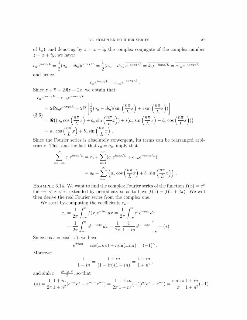
Example 3.14. We want to find the complex Fourier series of the function f(x) = ex
for −π < x < π, extended by periodicity so as to have f(x) = f(x + 2π). We willthen derive the real Fourier series from the complex one.
We start by computing the coefficients cn.
cn =1
2π
∫ π
−πf(x)e−inx dx =
1
2π
∫ π
−πexe−inx dx
=1
2π
∫ π
−πe(1−in)x dx =
1
2π
1
1− ine(1−in)x
∣∣∣∣π−π
= (∗)
Since cosx = cos(−x), we have
e±inπ = cos(±nπ) + i sin(±nπ) = (−1)n .
Moreover1
1− in=
1 + in
(1− in)(1 + in)=
1 + in
1 + n2,
and sinhx = ex−e−x2
, so that
(∗) =1
2π
1 + in
1 + n2(einπeπ − e−inπe−π) =
1
2π
1 + in
1 + n2(−1)n(eπ − e−π) =
sinhπ
π
1 + in
1 + n2(−1)n .
38 3. FOURIER ANALYSIS
Hence we can write the complex Fourier series of ex as
ex =sinhπ
π
∞∑n=−∞
(−1)n1 + in
1 + n2einx .
In order to find the real Fourier series, we just need to apply (3.6).
cneinx + c−ne
−inx = 2sinhπ
π<(−1)n
1 + in
1 + n2einx
=2 sinhπ
π(−1)n<
(1 + in
1 + n2(cosnx+ i sinnx)
)=
2 sinhπ
π(−1)n
(1
1 + n2cosnx− n
1 + n2sinnx
)Since c0 = 2 sinhπ
π, the real Fourier series of ex with period 2π is
ex =2 sinhπ
π+
2 sinhπ
π
∞∑n=1
(−1)n(
1
1 + n2cosnx− n
1 + n2sinnx
).
3.4. Approximation by trigonometric polynomials
We saw already that a trigonometric polynomial is defined as
A0 +N∑n=1
(An cosnx+Bn sinnx) ,
where N is the degree of the polynomial. So, for example the partial sums of aFourier series are a particular case of a trigonometric polynomial.
Given for simplicity f(x) periodic of period 2π, one wants to find what is thetrigonometric polynomial that “best approximates” f(x). We are not interested inpointwise approximation but we want an “overall best approximation”.
Let F (x) = A0 +∑N
n=1(An cosnx+Bn sinnx) and let us define the square errorin the approximation of f by F as
E =
∫ π
−π(f − F )2 dx .
A careful calculation using the orthogonality relations of the trigonometric systemshows the following:
Theorem 3.15. The trigonometric polynomial of degree N that best approximatesa function f on the interval [−π, π] (i.e. with the smallest square error) is the partialsum of the Fourier series of f . The minimum value E∗ of the square error is
E∗ =
∫ π
−πf 2 dx− π
[2a2
0 +N∑n=1
(a2n + b2
n)
]and it decreases as N increases.
3.5. FOURIER INTEGRAL 39
As an exercise, compute the minimum square error for the sawtooth wave (seeEx. 1 on page 505 of Kreyszig’s book).
3.5. Fourier integral
We see now how to extend the concept of Fourier series expansion to functionsthat are not periodic but defined on the whole real line (and hence cannot be ex-tended by periodicity). If f is periodic of period 2L, then we can write
f(x) = a0 +∞∑n=1
(an cos
(nπLx)
+ bn sin(nπLx))
=1
2L
∫ L
−Lf(v) dv +
∞∑n=1
[(1
L
∫ L
−Lf(v) cos
(nπLv)dv
)cos(nπLx)
+
(1
L
∫ L
−Lf(v) sin
(nπLv)dv
)sin(nπLx)]
.
We set now wn := nπL
so that ∆w = wn+1 − wn = πL
, and we obtain
f(x) =1
2L
∫ L
−Lf(v) dv +
1
L
∞∑n=1
[(∫ L
−Lf(v) cos(wnv) dv
)cos(wnx)+(∫ L
−Lf(v) sin(wnv) dv
)sin(wnx)
]=
1
2L
∫ L
−Lf(v) dv +
1
π
∞∑n=1
[(∫ L
−Lf(v) cos(wnv) dv
)cos(wnx)∆w+(∫ L
−Lf(v) sin(wnv) dv
)sin(wnx)∆w
].
We assume that f is absolutely integrable on R, that is that∫ ∞−∞|f(x)| dx <∞ .
(We recall that∫∞−∞ |f(x)| dx = limα→−∞
∫ oα|f(x)| dx+ limβ→∞
∫ β0|f(x)| dx.) From
this is follows that if L → ∞ the first term goes to 0 and ∆w → 0, so the sum onthe right becomes an integral
f(x) =1
π
∫ ∞0
[(∫ ∞−∞
f(v) coswv dv
)coswx+
(∫ ∞−∞
f(v) sinwv dv
)sinwx
]dw
=
∫ ∞0
[A(w) cos(wx) +B(w) sin(wx)] dw = f(x) ,
40 3. FOURIER ANALYSIS
where
A(w) :=1
π
∫ ∞−∞
f(v) cos(wv) dv
and
B(w) :=1
π
∫ ∞−∞
f(v) sin(wv) dv
This representation of f is called the Fourier integral of f .Just like for the Fourier series, one has to be careful to see whether the Fourier
integral actually represents the function. This happens if:
(1) f is piecewise continuous in finite intervals;(2) f has left and right derivatives at the points of discontinuity;(3) f if absolutely integrable.
Then the Fourier integral represents f at all points where f is continuous and con-verges toward the average of f at the points of discontinuity. The behaviour isanalogous as for the Fourier series.
Remark 3.16. The partial sums of a Fourier series correspond to integrals on finiteintervals
∫ a0
.
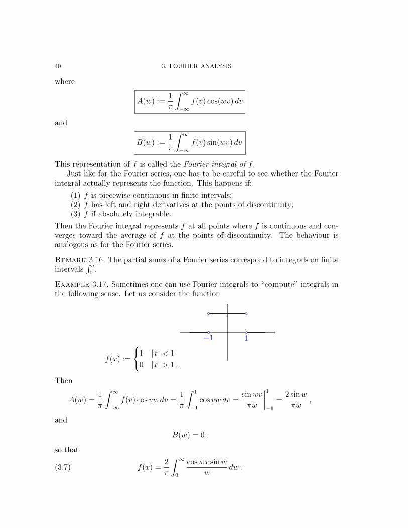
Example 3.17. Sometimes one can use Fourier integrals to “compute” integrals inthe following sense. Let us consider the function
f(x) :=
{1 |x| < 1
0 |x| > 1 .
−1 1
Then
A(w) =1
π
∫ ∞−∞
f(v) cos vw dv =1
π
∫ 1
−1
cos vw dv =sinwv
πw
∣∣∣∣1−1
=2 sinw
πw,
and
B(w) = 0 ,
so that
f(x) =2
π
∫ ∞0
coswx sinw
wdw .(3.7)
3.5. FOURIER INTEGRAL 41
Since the average of the left and the right limit of f at x = 1 is 12
= 1+02
, comparing(3.7) with the definition of the function f ,
∫ ∞0
coswx sinw
wdw =
π2|x| < 1
π4|x| = 1
0 |x| > 1 . �
This is called Dirichlet’s discontinuous factor. For x = 0 it becomes∫ ∞0
sinw
wdw =
π
2,
and
Si(u) =
∫ u
0
sinw
wdw
is called the sine integral.
3.5.1. Fourier sine and Fourier cosine integrals. Just like for the Fourierseries, we can simplify the formulas of the Fourier integral if the function is even orodd.
If f is even , then
A(w) =2
π
∫ ∞0
f(v) coswv dv
B(w) = 0
and
f(x) =
∫ ∞0
A(w) coswxdw ,
while if f is odd , then
A(w) = 0
B(w) =2
π
∫ ∞0
f(v) sinwv dv
and
f(x) =
∫ ∞0
B(w) sinwxdw .
42 3. FOURIER ANALYSIS
3.6. Fourier transform
There is another, and more common, form of the Fourier integral, one thatcorresponds to the complex form of the Fourier series.
f(x) =
∫ ∞0
(A(w) coswx+B(w) sinwx) dw
=1
π
∫ ∞0
∫ ∞−∞
f(v)(coswv coswx+ sinwv sinwx︸ ︷︷ ︸cos(wx−wv)
) dv dw
=1
π
∫ ∞0
∫ ∞−∞
f(v) cos(wx− wv) dv dw
=1
2π
∫ ∞−∞
∫ ∞−∞
f(v) cos(wx− wv) dv dw ,
where we used that
cos(wx− wv) = coswv coswx+ sinwv sinwx
is an even function of w.Likewise, since sin(wx− wv) is an odd function of w, we have that
1
2π
∫ ∞−∞
∫ ∞−∞
f(v) sin(wx− wv) dv dw = 0 ,
so that we can write
f(x) =1
2π
∫ ∞−∞
∫ ∞−∞
f(v) (cos(wx− wv) + i sin(wx− wv))︸ ︷︷ ︸eiw(x−v)
dv dw
=1
2π
∫ ∞−∞
∫ ∞−∞
f(v)eiw(x−v) dv dw
=1√2π
∫ ∞−∞
(1√2π
∫ ∞−∞
f(v)e−iwv dv
)eiwx dw .
Definition 3.18. The Fourier transform F(f) of f is defined as
F(f)(w) :=1√2π
∫ ∞−∞
f(v)e−iwv dv .
We denote the Fourier transform either as F(f) or as f(w). In either cases wehave that
f(x) =1√2π
∫ ∞−∞
f(w)eiwx dw
=1√2π
∫ ∞−∞F(f)(w)eiwx dw .
3.6. FOURIER TRANSFORM 43
Just like the Laplace transform, the Fourier transform is an integral transform widelyused in the engineering sciences.
Remark 3.19. Using the Fourier sine and cosine integral, one can define in ananalogous way the Fourier sine and cosine transforms.
The above formula gives also a formula for the inverse Fourier transform of afunction g(w), namely
F−1(g)(x) :=1√2π
∫ ∞−∞
g(w)eiwx dw ,
where the name “inverse Fourier transform” comes from the fact that if g = F(f),then
F−1(F(f)) = f .
As for the existence of the Fourier transform of a function f , we remark that if fis absolutely integrable and piecewise continuous on finite intervals, then its Fouriertransform exists.
Example 3.20. We compute the Fourier transform f of the function in Example 3.17
f(x) :=
{1 |x| < 1
0 |x| > 1 .
Applying the definition, we obtain
f(w) =1√2π
∫ ∞−∞
f(x)e−ixw dx =1√2π
∫ 1
−1
e−ixw dx
=1
−iw√
2πe−ixw
∣∣∣∣1−1
=−1
iw√
2π(e−iw − eiw)
=2 sinw
w√
2π=
√2
π
sinw
w.
Example 3.21. We compute the Fourier transform of the function
f(x) :=
{e−ax x > 0
0 x < 0,
where a > 0.
f(w) =1√2π
∫ ∞0
e−axe−iwx dx =1√2π
∫ ∞0
e−(a+iw)x dx
=1√2π
1
−(a+ iw)e−(a+iw)x
∣∣∣∣∞0
=1√
2π(a+ iw),
44 3. FOURIER ANALYSIS
where we used the fact that
limx→∞
e−(a+iw)x = limx→∞
e−ax(coswx+ i sinwx) = 0 ,
since limx→∞ e−ax = 0 and coswx+ i sinwx is bounded in absolute value.
Properties (Properties of the Fourier transform). (1) (Linearity)
F(αf + βg) = αF(f) + βF(g)
if all the Fourier transforms exist.(2) (Fourier transform of a derivative) If f is continuous on R, lim|x|→∞ f(x) = 0
and f ′ is absolutely integrable, then
F(f ′(x)) = iwF(f(x)) .(3.8)
(3) If f and g are piecewise continuous, bounded and absolutely integrable,then
F(f ∗ g) =√
2πF(f)F(g) .
Example 3.22. As an application of the properties of the Fourier transform, weassume we known that
F(e−ax2
) =1√2ae−w
2/4a .
and we compute F(xe−x2).
F(xe−x2
) = F(d
dx
(−1
2e−x
2
))= iwF
(−1
2e−x
2
)= −iw
2F(e−x
2
) = −iw2
1√2e−w
2/4 =−iw2√
2e−w
2/4 .
CHAPTER 4
Partial Differential Equations
4.1. Introduction and basic definitions
A partial differential equation (PDE in short) is an equation involving an un-known function and some of its partial derivatives. The unknown function dependson more than one variable, one of which can be the time and the others are spacevariables.
Example 4.1. uxyuz + utt = g(x, y, t). �
A PDE is called linear if the unknown function u and its derivatives appear withdegree one.
Example 4.2. The PDE uxyuz + utt = g(x, y, t) is not linear, but uxy + uz + utt =g(x, y, t) is. �
A linear PDE is called homogeneous if each of its terms contains either thefunction or one of its derivatives.
Example 4.3. The PDE uxy + uz + utt = g(x, y, t) is not homogeneous, but uxy +uz + utt = 0 is. �
The order of a PDE is the order of the highest derivative in the PDE. We willbe mostly concerned with second order PDEs.
Example 4.4. (1) One dimensional wave equation:
∂2u
∂t2= c2∂
2u
∂x2.
(2) One dimensional heat equation:
∂u
∂t= c2∂
2u
∂x2.
(3) Two dimensional Laplace equation:
∂2u
∂x2+∂2u
∂y2= 0 .
(4) Two dimensional Poisson equation:
∂2u
∂x2+∂2u
∂y2= f(x, y) .
45
46 4. PARTIAL DIFFERENTIAL EQUATIONS
(5) Two dimensional wave equation:
∂2u
∂t2= c2
(∂2u
∂x2+∂2u
∂y2
).
(6) Three dimensional Laplace equation:
∂2u
∂x2+∂2u
∂y2+∂2u
∂z2= 0 .
Here c is a positive real constant, x, y, z are spacial variables and the “dimension”refers to the number of spacial variables in the PDE. �
Remark 4.5. We will see later (for a class of PDEs a bit wider than the linear PDEsof second order) that linear PDEs of the second order can be classified into threegroups. In the above Examples 4.4(1)-(4), we could write each equation as
Auxx + 2Buxy + Cuyy = F (x, y, u, ux, uy) .(4.1)
(1) Set y = ct and obtain uyy − uxx = 0, that is A = −1 = −C, B = F = 0.(2) Set y = c2t and obtain uy−uxx = 0, that is A = 1, B = C = 0, and F = uy.(3) Here the PDE is already in the form (4.1), with A = C = 1 and B = F = 0.(4) Also here the PDE is already in the form (4.1), but now with A = C = 1,
B = 0 and F = f .
For the equations in Example 4.4(5) and (6), one could consider a general formsimilar to (4.1) but with more variables.
Now consider the polynomial
Ax2 + 2Bxy + Cy2 = L(x, y) ,(4.2)
where L is a linear function of x and y. We look at the discriminant.
(1) AC −B2 < 0, the curve in (4.2) is a hyperbola;(2) AC −B2 = 0, the curve in (4.2) is (most of the times) a parabola;(3) AC −B2 > 0, the curve in (4.2) is an ellipse.
We adopt the same denomination for the corresponding PDE, that are hence hyper-bolic, parabolic or elliptic. The reason to classify the second order linear PDEs inthis way it that each “group” of PDE has similar features that we will study later.
Example 4.6. (1) Wave equations are the prototypes of hyperbolic PDEs;(2) Heat equations are the prototypes of parabolic PDEs;(3) Laplace equations are the prototypes of elliptic PDEs. Given that the type
of a PDE depends only on the terms of second order, Poisson equations arealso elliptic.
This classification is independent of the dimension of the PDE, although ourmethod to derive the classification was not. �
A solution of a PDE in a region R is a function differentiable “enough times” inR and satisfying the PDE in R.
4.2. FROM A VIBRATING STRING TO THE WAVE EQUATION 47
Warning. Sometimes some care might need to be used on the boundary of theregion R. This can be done by insuring that R (in fact the boundary ∂R or R) iscontained in a slightly larger region where the function has enough derivatives.
Notice that the space of solutions of a PDE can be enormous.
Example 4.7. Any function of the form
u(x, t) = φ(x+ ct) + ψ(x− ct)
is a solution of the one-dimensional wave equation utt = c2uxx. In fact, uxx = u and
φt = cφ′ φtt = c2φ′′
ψt = −cψ′ ψtt = c2ψ′′ .
so that utt = φtt + ψtt = c2(φ′′ + ψ′′) = c2uxx.This means that any function of x + ct and x − ct is a solution, for example
u(x, t) = (x+ ct)1/3 + ex−ct or u(x, t) = cos(x+ ct) + (x− ct)n, or... �
In order to have uniqueness of solutions, we need to impose boundary conditionsor initial conditions. As the words say, the first are prescribed values of the solutionor of its derivatives on the boundary of the region R, while the second are givenvalues of the solution at a given time.
Another tool used to find solutions of a PDE is the following absolutely crucialprinciple:
Superposition Principle. If u1 and u2 are solutions of a homogeneous PDE, thenαu1 + βu2 is also a solution of the same PDE for all α, β ∈ R.
It is absolutely essential that the PDE be homogeneous.
4.2. From a vibrating string to the wave equation
Given a physical system whose behaviour we want to analyse, one of the firststep is to device an equation that describes the behaviour. The equation has tobe simple enough to be able to solve it (maybe numerically) but also such that thesolution will describe faithfully the system.
Take an elastic string stretched to have length L and tighten the endpoints. Weset the left endpoint to be at the origin of a system of Cartesian coordinates anddenote by u(x, t) the displacement of a point on the string above the point (x, 0)and at time t. We assume that
(1) the string movement happens only on one plane, say a vertical one, andevery point on the string moves only vertically;
(2) the string is homogenous (that is the mass per unit length ρ is constant),elastic and offers no resistance to bending;
(3) the tension is such that the effect of gravity is negligible.
48 4. PARTIAL DIFFERENTIAL EQUATIONS
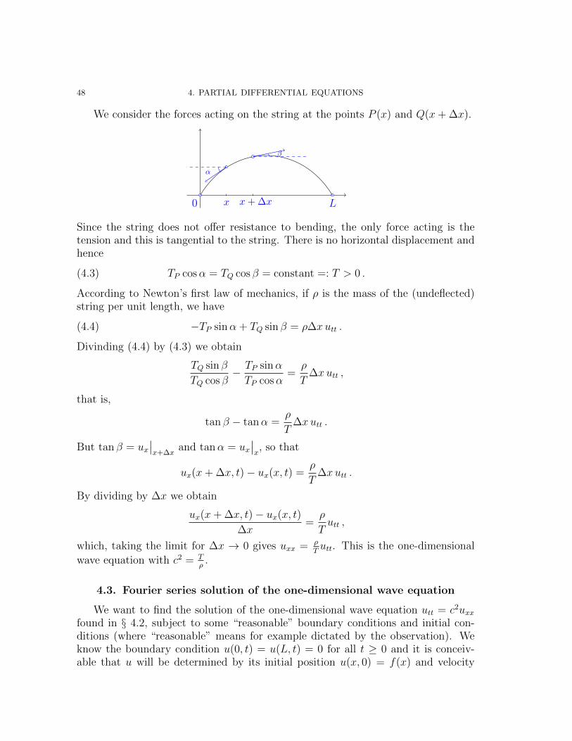
We consider the forces acting on the string at the points P (x) and Q(x+ ∆x).
0 Lx
α
x+ ∆x
β
Since the string does not offer resistance to bending, the only force acting is thetension and this is tangential to the string. There is no horizontal displacement andhence
TP cosα = TQ cos β = constant =: T > 0 .(4.3)
According to Newton’s first law of mechanics, if ρ is the mass of the (undeflected)string per unit length, we have
−TP sinα + TQ sin β = ρ∆xutt .(4.4)
Divinding (4.4) by (4.3) we obtain
TQ sin β
TQ cos β− TP sinα
TP cosα=ρ
T∆xutt ,
that is,
tan β − tanα =ρ
T∆xutt .
But tan β = ux∣∣x+∆x
and tanα = ux∣∣x, so that
ux(x+ ∆x, t)− ux(x, t) =ρ
T∆xutt .
By dividing by ∆x we obtain
ux(x+ ∆x, t)− ux(x, t)∆x
=ρ
Tutt ,
which, taking the limit for ∆x → 0 gives uxx = ρTutt. This is the one-dimensional
wave equation with c2 = Tρ.
4.3. Fourier series solution of the one-dimensional wave equation
We want to find the solution of the one-dimensional wave equation utt = c2uxxfound in § 4.2, subject to some “reasonable” boundary conditions and initial con-ditions (where “reasonable” means for example dictated by the observation). Weknow the boundary condition u(0, t) = u(L, t) = 0 for all t ≥ 0 and it is conceiv-able that u will be determined by its initial position u(x, 0) = f(x) and velocity
4.3. FOURIER SERIES SOLUTION OF THE ONE-DIMENSIONAL WAVE EQUATION 49
u′(x, 0) = g(x), for all 0 ≤ x ≤ L. Hence we want to solve the systemutt = c2uxx
u(0, t) = u(L, t) = 0 t ≥ 0
u(x, 0) = f(x) 0 ≤ x ≤ L
ut(x, 0) = g(x) 0 ≤ x ≤ L .
(4.5)
The first method we want to study consists in three steps:
1. Separation of variables;2. Determination of “many” intermediary solutions;3. Use of Fourier series “to put together” the solutions.
4.3.1. Separation of variables. Suppose there exists a solution of the form
u(x, t) = F (x)G(t) .
Then utt = FG and uxx = F ′′G, so that
FG = c2F ′′G ,
from which it follows that
G
c2G=F ′′
F.
Since the right hand side of the equation does not depend on t, it follows that eventhe left hand side is independent of t, and hence constant. Thus the right hand sideis a constant as well
G
c2G=F ′′
F= k ,
which is equivalent to the system of two equations{F ′′ = kF
G = c2kG .(4.6)
Thus, assuming that there is a solution of the PDE in (4.5) of the form u(x, t) =F (x)G(t), the two functions F and G must satisfy (4.6). The type of solution willdepend on the sign of the constant k. We start by solving the ordinary differentialequation that has homogeneous boundary conditions. In other words the boundarycondition for such a solution u(x, t) = F (x)G(t) get transformed into
u(0, t) = F (0)G(t) = 0 for every t ≥ 0⇒ F (0) = 0
u(L, t) = F (L)G(t) = 0 for every t ≥ 0⇒ F (L) = 0 .
50 4. PARTIAL DIFFERENTIAL EQUATIONS
4.3.2. Determination of “many” solutions. Hence we start looking for afunction F (x) that is a solution of the system
F ′′ = kF , with F (0) = F (L) = 0 .(4.7)
k = 0 Then the ODE becomes F ′′ = 0, which has solution F (x) = ax + b. Ifwe impose the conditions F (0) = F (L) = 0 we see that F (x) must beidentically equal to zero and this is not an interesting solution.
k > 0 Then the theory of the solutions of linear second order ODEs with constant
coefficients tells us that the general solution is F (x) = Ae√kx + Be−
√kx.
Imposing the initial conditions we deduce from F (0) = 0 that A + B = 0
and from F (L) = 0 that Ae√kL + Be−
√kL = 0. Replacing B = −A in
the second equation we obtain that A(e√kL − e−
√kL) = 0. Then either
A = B = 0 and this is again the zero solution or e2√kL = 1, that is
impossible since k 6= 0.k < 0 In this case we know that
F (x) = A cos(√−k x) +B sin(
√−k x) .
Again imposing the initial conditions we obtain that 0 = F (0) = A and0 = F (L) = B sin(
√−kL). If B = 0 then F is again the solution that is
identically equal to zero. So it must be sin(√−kL) = 0, that is
√−kL = nπ
for any n ∈ N or√−k = nπ
Lfor any n ∈ N. Hence for every n ∈ N there is
a solution
Fn(x) = sin(nπLx)
of (4.7), where√−k = nπ
L.
For these values of k we look for a solution of G = c2kG, that is we look for a
solution of G = −c2(nπL
)2G. We obtain
Gn(t) = Bn cos(cnπLt)
+B∗n sin(cnπLt)
= Bn cos(λnt) +B∗n sin(λnt) ,
where λn = cnπL
.We have thus found a family of solutions indexed by n ∈ N, namely
un(x, t) =(Bn cos(λnt) +B∗n sin(λnt)
)sin(nπLx).(4.8)
The functions un are the eigenfunctions of the vibrating string with eigenvaluesλn = cnπ
L. The set {λ1, λ2, . . . , } is called the spectrum.
4.3. FOURIER SERIES SOLUTION OF THE ONE-DIMENSIONAL WAVE EQUATION 51
4.3.3. Use of Fourier series. Each of the eigenfunctions un satisfies the PDEin (4.5) and the boundary conditions,{
utt = c2uxx
u(0, t) = u(L, t) = 0 t ≥ 0 .(4.9)
However, most of the times, each one of them will not satisfy the initial conditionsu(x, 0) = f(x) and ut(x, 0) = g(x). Since the PDE is homogeneous, we can use thesuperposition principle. Without worrying too much about convergence issues, wecan say that the function
u(x, t) :=∞∑n=1
un(x, t) =∞∑n=1
(Bn cos(λnt) +B∗n sin(λnt)
)sin(nπLx)
is also a solution of (4.9) and now we have many coefficients that we can determineso that u(x, t) satisfies also the initial conditions. With this solution the first initialcondition about u becomes
f(x) = u(x, 0) =∞∑n=1
Bn sin(nπLx).(4.10)
where the series on the right hand side is the sine series of an odd 2L-periodicfunction that coincides with f on [0, L]. So if we extend f to be odd and 2L-periodic, we have
Bn =2
L
∫ L
0
f(x) sin(nπLx)dx ,
for n ≥ 1, n ∈ N. Moreover the initial condition on the derivative u′ becomes
g(x) = ut(x, 0)
=∞∑n=1
(− λnBn sin(λnt) + λnB
∗n cos(λnT )
)sin(nπLx) ∣∣∣∣
t=0
=∞∑n=1
λnB∗n sin
(nπLx).
Just like in the case of (4.10), this is nothing but the Fourier series of the function g,extended to be odd and periodic of period 2L, so that the formula for the coefficientsgives us
λnB∗n =
2
L
∫ L
0
g(x) sin(nπLx)dx ,
or
B∗n =2
Lλn
∫ L
0
g(x) sin(nπLx)dx .
52 4. PARTIAL DIFFERENTIAL EQUATIONS
Remark 4.8. Let us assume for simplicity that g = 0. Recalling that λn = cnπL
, thesolution u(x, t) becomes
u(x, t) =∞∑n=1
Bn cos(λnt) sin(nπLx)
=∞∑n=1
Bn1
2
[sin(nπLx− λnt
)+ sin
(nπLx+ λnt
)]=
1
2
∞∑n=1
Bn
[sin
nπ
L(x− ct) + sin
nπ
L(x+ ct)
]=
1
2
∞∑n=1
Bn sinnπ
L(x− ct) +
1
2
∞∑n=1
Bn sinnπ
L(x+ ct)
=1
2[f ∗(x− ct) + f ∗(x+ ct)] ,
(4.11)
where f ∗ is the odd extension of f to a 2L-periodic function.If
(1) f is twice differentiable on 0 < x < L and(2) f has one-sided zero second derivative at the endpoints,
then u is a solution for all 0 ≤ x ≤ L.If f is only piecewise twice differentiable or the one-sided derivatives are not
zero, then u is a solution for all 0 ≤ x ≤ L except at the points x where f is nottwice differentiable.
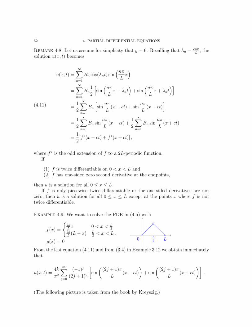
Example 4.9. We want to solve the PDE in (4.5) with
f(x) =
{2kLx 0 < x < L
22kL
(L− x) L2< x < L .
g(x) = 0 0 L2 L
From the last equation (4.11) and from (3.4) in Example 3.12 we obtain immediatelythat
u(x, t) =4k
π2
∞∑j=0
(−1)j
(2j + 1)2
[sin
((2j + 1)π
L(x− ct)
)+ sin
((2j + 1)π
L(x+ ct)
)].
(The following picture is taken from the book by Kreyszig.)
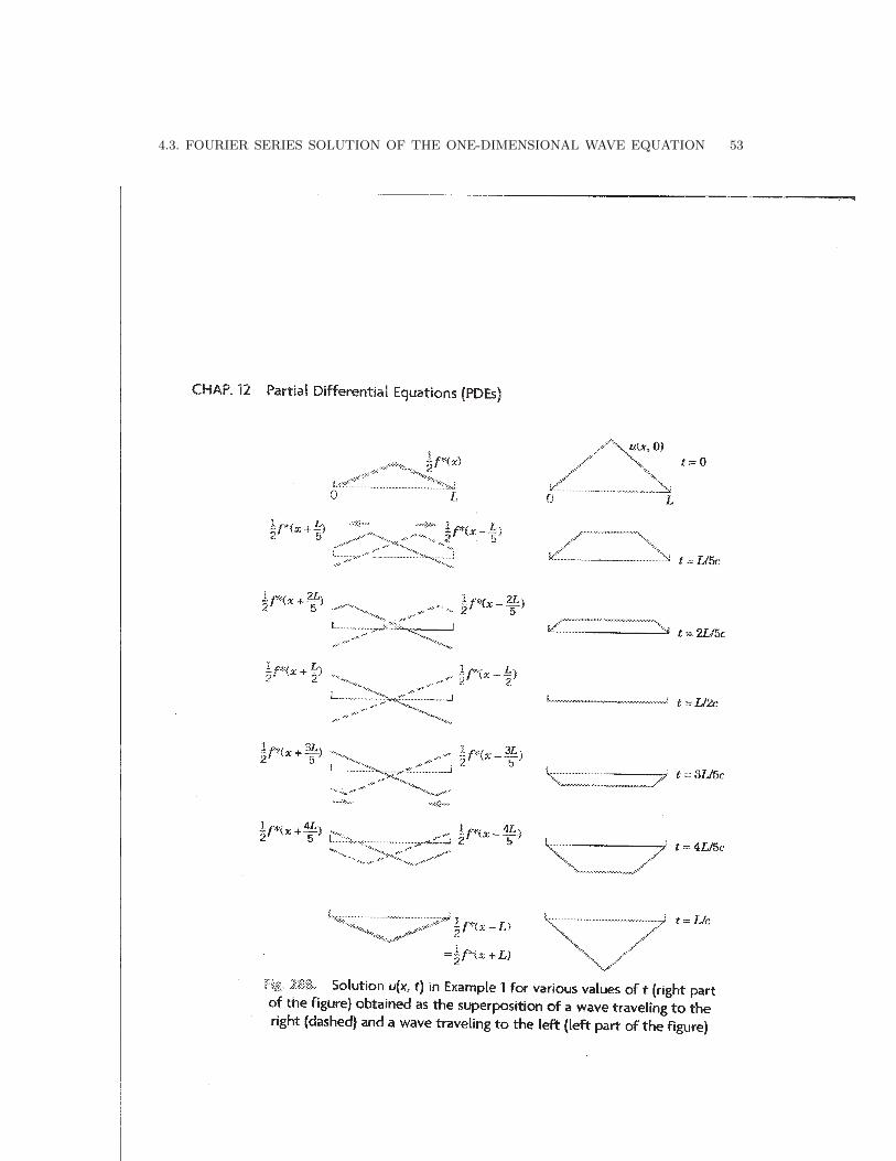
4.3. FOURIER SERIES SOLUTION OF THE ONE-DIMENSIONAL WAVE EQUATION 53
54 4. PARTIAL DIFFERENTIAL EQUATIONS
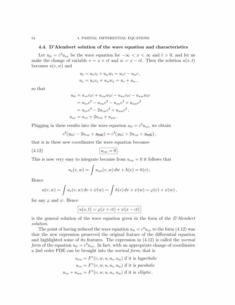
4.4. D’Alembert solution of the wave equation and characteristics
Let utt = c2uxx be the wave equation for −∞ < x < ∞ and t > 0, and let usmake the change of variable v = x + ct and w = x − ct. Then the solution u(x, t)becomes u(v, w) and
ut = uvvt + uwwt = uvc− uwc ,ux = uvvx + uwwx = uv + uw ,
so that
utt = uvvvtc+ uvwwtc− uwvvtc− uwwwtc= uvvc
2 − uvwc2 − uwvc2 + uwwc2
= uvvc2 − 2uvwc
2 + uwwc2 ,
uxx = uvv + 2uvw + uww .
Plugging in these results into the wave equation utt = c2uxx, we obtain
c2(��uvv − 2uvw +���XXXuww ) = c2(��uvv + 2uvw +���XXXuww ) ,
that is in these new coordinates the wave equation becomes
uvw = 0 .(4.12)
This is now very easy to integrate because from uvw = 0 it follows that
uv(v, w) =
∫uvw(v, w) dw + h(v) = h(v) ;
Hence
u(v, w) =
∫uv(v, w) dv + ψ(w) =
∫h(v) dv + ψ(w) = ϕ(v) + ψ(w) ,
for any ϕ and ψ. Hence
u(x, t) = ϕ(x+ ct) + ψ(x− ct)
is the general solution of the wave equation given in the form of the D’Alembertsolution.
The point of having reduced the wave equation utt = c2uxx to the form (4.12) wasthat the new expression preserved the original feature of the differential equationand highlighted some of its features. The expression in (4.12) is called the normalform of the equation utt = c2uxx. In fact, with an appropriate change of coordinatesa 2nd order PDE can be brought into the normal form, that is
uvw = F ∗(v, w, u, uv, uw) if it is hyperbolic
uvv = F ∗(v, w, u, uv, uw) if it is parabolic
uvv + uww = F ∗(v, w, u, uv, uw) if it is elliptic .
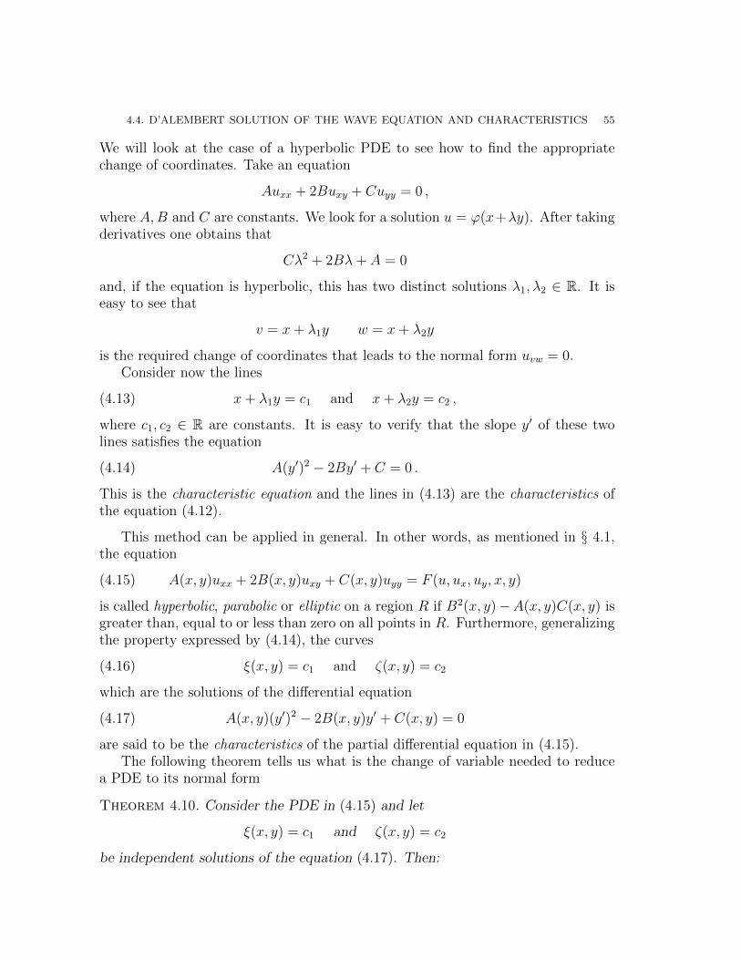
4.4. D’ALEMBERT SOLUTION OF THE WAVE EQUATION AND CHARACTERISTICS 55
We will look at the case of a hyperbolic PDE to see how to find the appropriatechange of coordinates. Take an equation
Auxx + 2Buxy + Cuyy = 0 ,
where A,B and C are constants. We look for a solution u = ϕ(x+λy). After takingderivatives one obtains that
Cλ2 + 2Bλ+ A = 0
and, if the equation is hyperbolic, this has two distinct solutions λ1, λ2 ∈ R. It iseasy to see that
v = x+ λ1y w = x+ λ2y
is the required change of coordinates that leads to the normal form uvw = 0.Consider now the lines
x+ λ1y = c1 and x+ λ2y = c2 ,(4.13)
where c1, c2 ∈ R are constants. It is easy to verify that the slope y′ of these twolines satisfies the equation
A(y′)2 − 2By′ + C = 0 .(4.14)
This is the characteristic equation and the lines in (4.13) are the characteristics ofthe equation (4.12).
This method can be applied in general. In other words, as mentioned in § 4.1,the equation
A(x, y)uxx + 2B(x, y)uxy + C(x, y)uyy = F (u, ux, uy, x, y)(4.15)
is called hyperbolic, parabolic or elliptic on a region R if B2(x, y)−A(x, y)C(x, y) isgreater than, equal to or less than zero on all points in R. Furthermore, generalizingthe property expressed by (4.14), the curves
ξ(x, y) = c1 and ζ(x, y) = c2(4.16)
which are the solutions of the differential equation
A(x, y)(y′)2 − 2B(x, y)y′ + C(x, y) = 0(4.17)
are said to be the characteristics of the partial differential equation in (4.15).The following theorem tells us what is the change of variable needed to reduce
a PDE to its normal form
Theorem 4.10. Consider the PDE in (4.15) and let
ξ(x, y) = c1 and ζ(x, y) = c2
be independent solutions of the equation (4.17). Then:
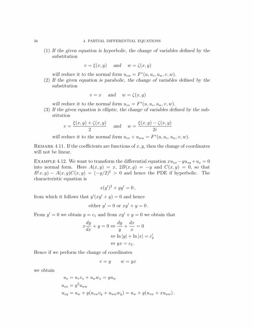
56 4. PARTIAL DIFFERENTIAL EQUATIONS
(1) If the given equation is hyperbolic, the change of variables defined by thesubstitution
v = ξ(x, y) and w = ζ(x, y)
will reduce it to the normal form uvw = F ∗(u, uv, uw, v, w).(2) If the given equation is parabolic, the change of variables defined by the
substitution
v = x and w = ζ(x, y)
will reduce it to the normal form uvv = F ∗(u, uv, uw, v, w).(3) If the given equation is elliptic, the change of variables defined by the sub-
stitution
v =ξ(x, y) + ζ(x, y)
2and w =
ξ(x, y)− ζ(x, y)
2i
will reduce it to the normal form uvv + uww = F ∗(u, uv, uw, v, w).
Remark 4.11. If the coefficients are functions of x, y, then the change of coordinateswill not be linear.
Example 4.12. We want to transform the differential equation xuxx−yuxy+ux = 0into normal form. Here A(x, y) = x, 2B(x, y) = −y and C(x, y) = 0, so thatB(x, y) − A(x, y)C(x, y) = (−y/2)2 > 0 and hence the PDE if hyperbolic. Thecharacteristic equation is
x(y′)2 + yy′ = 0 ,
from which it follows that y′(xy′ + y) = 0 and hence
either y′ = 0 or xy′ + y = 0 .
From y′ = 0 we obtain y = c1 and from xy′ + y = 0 we obtain that
xdy
dx+ y = 0⇔ dy
y+dx
x= 0
⇔ ln |y|+ ln |x| = c′2⇔ yx = c2 .
Hence if we perform the change of coordinates
v = y w = yx
we obtain
ux = uvvx + uwwx = yuw
uxx = y2uww
uxy = uw + y(uvwvy + uwwwy) = uw + y(uvw + xuww) .
4.4. D’ALEMBERT SOLUTION OF THE WAVE EQUATION AND CHARACTERISTICS 57
Plugging this into the original equation gives, after simplifying, uvw = 0. Henceu(v, w) = ϕ(v) + ψ(w) or
u(x, y) = ϕ(y) + ψ(xy) ,
where ϕ and ψ are arbitrary. �
Why are the characteristics important? Let us go back to the d’Alembert solutionof the wave equation,
u(x, t) = ϕ(x+ ct) + ψ(x− ct) for x ∈ R and t > 0 ,(4.18)
and let us assume that we want to satisfy the initial conditions
u(x, 0) = f(x) ut(x, 0) = g(x) for all x ∈ R(4.19)
The initial value problem consisiting of (4.18) and (4.19) is called Cauchy problemfor the one dimensional wave equation. A solution of this problem can be interpretedfor example as the amplitude of a sound wave propagating in a very long and narrowpipe.
To find the solution of (4.18) and (4.19), observe that for every y ∈ R{f(y) = ϕ(y) + ψ(y)
g(y) = cϕ′(y)− cψ′(y) ,
from which it follows thatϕ(y) + ψ(y) = f(y)
ϕ(y)− ψ(y) = 1c
∫ y0g(s) ds+
=:k0︷ ︸︸ ︷ϕ(0)− ψ(0) ,
⇒
{ϕ(y) = 1
2f(y) + 1
2c
∫ y0g(s) ds+ 1
2k0
ψ(y) = 12f(y)− 1
2c
∫ y0g(s) ds− 1
2k0 .
In particular evaluating the first expression for y = x + ct and the second for y =x− ct, we have
ϕ(x+ ct) =1
2f(x+ ct) +
1
2c
∫ x+ct
0
g(s) ds+1
2k0
ψ(x− ct) =1
2f(x− ct)− 1
2c
∫ x−ct
0
g(s) ds− 1
2k0
(4.20)
and hence
u(x, t) =1
2[f(x+ ct) + f(x− ct)] +
1
2c
∫ x+ct
x−ctg(s) ds ,
which is the d’Alembert solution of the Cauchy problem (4.18) and (4.19).
58 4. PARTIAL DIFFERENTIAL EQUATIONS
We are interested in investigating what kind of information has an influence onthe solution u at the point (x, t). Through any point (x0, t0) with t0 > 0, there areexactly two characteristics, namely
x− ct = x0 − ct0 and x+ ct = x0 + ct0 .
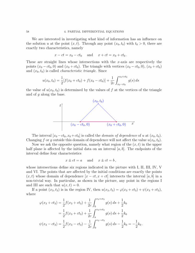
These are straight lines whose intersections with the x-axis are respectively thepoints (x0− ct0, 0) and (x0 + ct0). The triangle with vertices (x0− ct0, 0), (x0 + ct0)and (x0, t0) is called characteristic triangle. Since
u(x0, t0) =1
2[f(x0 + ct0) + f(x0 − ct0)] +
1
2c
∫ x0+ct0
x0−ct0g(s) ds
the value of u(x0, t0) is determined by the values of f at the vertices of the triangleand of g along the base.
x
t
(x0 − ct0, 0)
(x0, t0)
(x0 + ct0, 0)
The interval [x0−ct0, x0 +ct0] is called the domain of dependence of u at (x0, t0).Changing f or g outside this domain of dependence will not affect the value u(x0, t0).
Now we ask the opposite question, namely what region of the (x, t) in the upperhalf plane is affected by the initial data on an interval [a, b]. The endpoints of theinterval define four characteristics
x± ct = a and x± ct = b ,
whose intersections define six regions indicated in the picture with I, II, III, IV, Vand VI. The points that are affected by the initial conditions are exactly the points(x, t) whose domain of dependence [x − ct, x + ct] intersects the interval [a, b] in anon-trivial way. In particular, as shown in the picture, any point in the regions Iand III are such that u(x, t) = 0.
If a point (x3, t3) is in the region IV, then u(x3, t3) = ϕ(x3 + ct3) + ψ(x3 + ct3),where
ϕ(x3 + ct3) =1
2f(x3 + ct3) +
1
2c
∫ x3+ct3
0
g(s) ds+1
2k0
=1
2f(x3 + ct3) +
1
2c
∫ x3+ct3
a
g(s) ds+1
2k0
ψ(x3 − ct3) =1
2f(x3 − ct3)− 1
2c
∫ x3−ct3
0
g(s) ds− 1
2k0 = −1
2k0 .
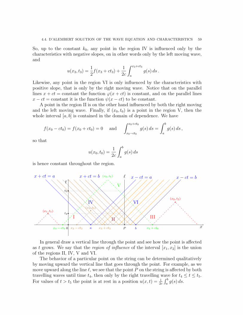
4.4. D’ALEMBERT SOLUTION OF THE WAVE EQUATION AND CHARACTERISTICS 59
So, up to the constant k0, any point in the region IV is influenced only by thecharacteristics with negative slopes, on in other words only by the left moving wave,and
u(x3, t3) =1
2f(x3 + ct3) +
1
2c
∫ x3+ct3
a
g(s) ds .
Likewise, any point in the region VI is only influenced by the characteristics withpositive slope, that is only by the right moving wave. Notice that on the parallellines x + ct = constant the function ϕ(x + ct) is constant, and on the parallel linesx− ct = constant it is the function ψ(x− ct) to be constant.
A point in the region II is on the other hand influenced by both the right movingand the left moving wave. Finally, if (x0, t0) is a point in the region V, then thewhole interval [a, b] is contained in the domain of dependence. We have
f(x0 − ct0) = f(x0 + ct0) = 0 and
∫ x0+ct0
x0−ct0g(s) ds =
∫ b
a
g(s) ds ,
so that
u(x0, t0) =1
2c
∫ b
a
g(s) ds
is hence constant throughout the region.
xa b
t
0
x− ct = ax+ ct = a x− ct = bx+ ct = b
(x1, t1)
(x2, t2)
x3 − ct3
(x3, t3)
x3 + ct3
(x0, t0)
x0 − ct0 x0 + ct0
`
P
t4
t5
I II III
IV VI
V
In general draw a vertical line through the point and see how the point is affectedas t grows. We say that the region of influence of the interval [x1, x2] is the unionof the regions II, IV, V and VI.
The behavior of a particular point on the string can be determined qualitativelyby moving upward the vertical line that goes through the point. For example, as wemove upward along the line `, we see that the point P on the string is affected by bothtravelling waves until time t4, then only by the right travelling wave for t4 ≤ t ≤ t5.
For values of t > t5 the point is at rest in a position u(x, t) = 12c
∫ bag(s) ds.
60 4. PARTIAL DIFFERENTIAL EQUATIONS
Remark 4.13. It follows from the above considerations that if at some point thereis a singularity, it will propagate for all t. This is typical of hyperbolic equations.
4.5. The Heat equation via Fourier series
Assume that we have an insulated bar of length L, positioned along the interval[0, L] of the x-axis, so that the heat flows only in the x-direction. We assume thatthe temperature at the endpoints of the bar is zero and, given an initial distributionof temperature f(x), we want to find the heat distribution of the bar at time t andposition x. In other words, we want now to solve the one-dimensional heat equation,that is
ut = c2uxxu(0, t) = u(L, t) = 0
u(x, 0) = f(x) ,
where c2 = Kσρ
, with K the thermal conductivity, σ the specific heat and ρ the
density of the bar. Here c is the thermal diffusivity that measures the ability of amaterial to conduct thermal energy relative to its ability to store thermal energy,(this is approximately analogous to whether a material is ”cold to the touch”).
As in the case of the wave equation, we look for a solution of the form
u(x, t) = F (x)G(t) .
Differentiating this with respect to t once and to x twice, and plugging it into theheat equation, we obtain
G
c2G=F ′′
F= k ,
where k is a constant due to the fact that each of the two fractions cannot dependon the only variable present. This leads to the two differential equations
F ′′ = kF , G = kc2G ,
with initial conditions
F (0) = F (L) = 0 .
Solving first
F ′′ = kF , F (0) = F (L) = 0 ,
as in the case of the wave equation we can easily argue that if k = 0 the only possiblesolution is the one identically zero and that if k > 0 there are no solutions. So k < 0and we can set k = −p2, so that the system to solve becomes
F ′′ = −p2F , F (0) = F (L) = 0 .(4.21)
The general solution is F (x) = A cos(px)+B sin(px). Imposing the initial conditionF (0) = 0 we obtain that A = 0; imposing the initial condition F (L) = 0 we obtain
4.5. THE HEAT EQUATION VIA FOURIER SERIES 61
that sin(pL) = 0, that is that pL = nπ for n ∈ Z, n ≥ 1. Hence p = nπL
. We havetherefore found the infinite family of solutions of (4.21)
Fn(x) = sin(nπLx), n ∈ N .
The corresponding differential equation for G is
G+ c2(nπL
)2
G = 0
whose solution is
Gn(t) = Bne−λ2nt ,
where λ2n =
(cnπL
)2. It follows that the functions
un(x, t) = Bn sin(nπLx)e−λ
2nt n ∈ N ,
with λn as above satisfies the conditions{ut = c2uxxu(0, t) = u(L, t) = 0 .
Because of the Superposition Principle, the function
u(x, t) =∞∑n=1
un(x, t) =∞∑n=1
Bn sin(nπLx)e−λ
2nt(4.22)
is also a solution. By imposing the initial condition u(x, 0) = f(x), we obtain
f(x) = u(x, 0) =∞∑n=1
Bn sin(nπLx).
Hence the Bn are the Fourier coefficients of the extension of f to be an odd functionperiodic of period 2L, that is
Bn =2
L
∫ L
0
f(x) sin(nπLx)dx .(4.23)
Hence (4.22) is the solution with the coefficients Bn given by (4.23) We remark thateach term in the Fourier series (4.22) goes to zero with time, and the larger the nis, the faster the decay is.
Example 4.14. We consider a copper bar of length 80 cm that is laterally insulated.The ends are kept at 0◦C and the initial temperature is f(x). We want to find u(x, t)and compute how long it will take for the maximum temperature to drop to 50◦Cin the two cases in which
(1) f(x) = 100 sin(πx80
), and
(2) f(x) = 100 sin(
3πx80
).
62 4. PARTIAL DIFFERENTIAL EQUATIONS
We recall that the density ρ of copper is 8.92 g/cm3, the specific heat σ is 0.092 cal/(g×◦C) and the thermal conductivity K is 0.95 cal/(cm× sec× ◦C), so that
c2 =K
σρ=
0.95
0.092× 8.92
cal
cm× sec× ◦Cg × ◦C
cal
cm3
g= 1.158
cm2
sec.
Solution. We have
(1a) u(x, 0) = 100 sin(πx80
)⇒ Bn = 0 for n ≥ 2 and B1 = 100;
(2a) u(x, 0) = 100 sin(
3πx80
)⇒ Bn = 0 for n = 1, 2 and n ≥ 4 and B3 = 100,
hence
(1b) λ21 = c2 π2
L2 = 1.1589.870802' 0.001785 sec−1;
(2b) λ23 = c2 9π2
L2 = 9λ1 ' 0.01607 sec−1,
from which it follows that
(1c) u(x, t) = 100 sin(πLx)e−0.001785t;
(2c) u(x, t) = 100 sin(
3πLx)e−0.01607t.
Thus
(1d) umax(x, t) = 100e−0.001785t;(2d) umax(x, t) = 100e−0.01607t,
and hence
(1e) 100e−0.001785t = 50⇒ t = ln 0.5/(−0.001785) ' 388 sec;(2e) 100e−0.01607t = 50⇒ t = ln 0.5/(−0.01607) ' 43 sec.
4.5.1. Steady two-dimensional heat equation and Laplace equation.The heat equation ut = c2∇2u reduces to ∇2u = 0 if the solution u does notdepend on time. This is the so-called Laplace equation. It governs not only theso-called steady-state solution of a heat equation (that is the solution after thesystem reaches its equilibrium and does not change anymore with time), but alsomany other phenomena in mechanics and electromagnetism, such as for instance theelectrostatic potential. This is an example of an elliptic equation and it comes withdifferent kinds of boundary conditions. Suppose for example that ∇2u = 0 holds ona region R.
• If u is prescribed on the boundary ∂R of R, then we have the Dirichletproblem;• If the partial derivative un of u in the direction n normal to ∂R is prescribed
on ∂R, then we have the Neumann problem;• If u is prescribed on one part of ∂R and un on another part of ∂R, we have
the Robin problem.
Dirichlet problem on a rectangle. We assume that the temperature u(x, y)on a rectangle R satisfies ∇2u = 0 and if
R = {(x, y) : 0 ≤ x ≤ a, 0 ≤ y ≤ b} ,
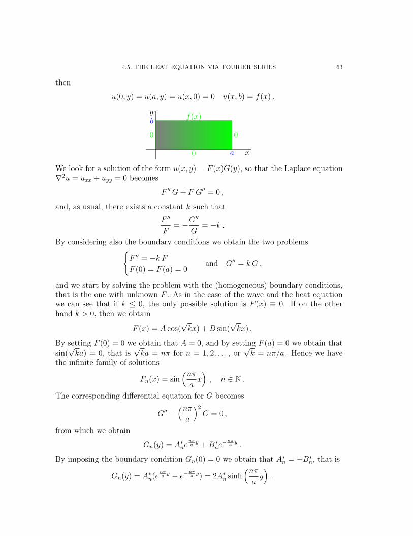
4.5. THE HEAT EQUATION VIA FOURIER SERIES 63
then
u(0, y) = u(a, y) = u(x, 0) = 0 u(x, b) = f(x) .
x
y
a
b
0 0
0
f(x)
We look for a solution of the form u(x, y) = F (x)G(y), so that the Laplace equation∇2u = uxx + uyy = 0 becomes
F ′′G+ F G′′ = 0 ,
and, as usual, there exists a constant k such that
F ′′
F= −G
′′
G= −k .
By considering also the boundary conditions we obtain the two problems{F ′′ = −k FF (0) = F (a) = 0
and G′′ = k G .
and we start by solving the problem with the (homogeneous) boundary conditions,that is the one with unknown F . As in the case of the wave and the heat equationwe can see that if k ≤ 0, the only possible solution is F (x) ≡ 0. If on the otherhand k > 0, then we obtain
F (x) = A cos(√kx) +B sin(
√kx) .
By setting F (0) = 0 we obtain that A = 0, and by setting F (a) = 0 we obtain that
sin(√ka) = 0, that is
√ka = nπ for n = 1, 2, . . . , or
√k = nπ/a. Hence we have
the infinite family of solutions
Fn(x) = sin(nπax), n ∈ N .
The corresponding differential equation for G becomes
G′′ −(nπa
)2
G = 0 ,
from which we obtain
Gn(y) = A∗nenπay +B∗ne
−nπay .
By imposing the boundary condition Gn(0) = 0 we obtain that A∗n = −B∗n, that is
Gn(y) = A∗n(enπay − e−
nπay) = 2A∗n sinh
(nπay).
64 4. PARTIAL DIFFERENTIAL EQUATIONS
Thus for every n ∈ N we have a solution
un(x, y) = An sin(nπax)
sinh(nπay),
and hence by the Superposition Principle
u(x, y) =∞∑n=1
un(x, y) =∞∑n=1
An sin(nπax)
sinh(nπay)
is a solution as well. To satisfy the last condition u(x, b) = f(x), we write
f(x) =∞∑n=1
[An sinh
(nπab)]
sin(nπax),
from which we deduce that An sinh(nπab)
is the Fourier coefficient of the extensionof f to be an odd periodic function of period 2a. In other words
An sinh(nπab)
=2
a
∫ a
0
f(x) sin(nπax)dx .
Hence the solution of the above Dirichlet problem is
u(x, y) =∞∑n=1
An sin(nπax)
sinh(nπay),
where
An =2
a sinh(nπab) ∫ a
0
f(x) sin(nπax)dx .
4.6. Heat equation on an infinite bar
This method is appropriate when we have an infinite domain, for example a barof infinite length. In this case the problem to solve is{
ut = c2uxx
u(x, 0) = f(x) .
We are going to modify the method that used the Fourier series in order to use theFourier integral. Then we will see also how one can use the Fourier transform. Welook again for a solution of the form
u(x, t) = F (x)G(t) ,
and we obtain
F (x)G(t) = c2F ′′(x)G(t) ,
from which, as usual,
F ′′(x)
F (x)=
1
c2
G(t)
G(t)= −k .
4.6. HEAT EQUATION ON AN INFINITE BAR 65
Hence the differential equations to solve are{F ′′(x) + kF (x) = 0
G(t) + c2kG(t) = 0 .
Even without boundary conditions we see that if k < 0, then{F (x) = Ae
√−kx +Be−
√−kx
G(t) = e−c2kt ,
from which u(x, t) = e−c2kt(Ae
√−kx +Be−
√−kx) will increase as t increases, which is
physically impossible. Thus k ≥ 0, and we can write k = p2. Then{Fp(x) = A(p) cos(px) +B(p) sin(px)
Gp(t) = e−c2p2t .
A generalisation of the Superposition Principle leads to the solution
u(x, t) =
∫ ∞0
[A(p) cos(px) +B(p) sin(px)]e−c2p2t dp .(4.24)
Since u(x, 0) = f(x), then
f(x) =
∫ ∞0
[A(p) cos(px) +B(p) sin(px)] dp ,
which is nothing but the Fourier integral of f . Hence we can determine the coeffi-cients A(p) and B(p), namely
A(p) =1
π
∫ ∞−∞
f(v) cos(pv) dv
B(p) =1
π
∫ ∞−∞
f(v) sin(pv) dv .
Plugging these into (4.24) and using the prostapheresis formulas, we obtain
u(x, t) =1
π
∫ ∞0
∫ ∞−∞
f(v)[cos(pv) cos(px) + sin(pv) sin(px)]e−c2p2t dv dp
=1
π
∫ ∞0
∫ ∞−∞
f(v) cos(px− pv)e−c2p2t dv dp
=1
π
∫ ∞−∞
f(v)
(∫ ∞0
cos(px− pv)e−c2p2t dp
)dv .
(4.25)
We assume for the moment that we know that∫ ∞0
cos(2bs)e−s2
ds =
√π
2e−b
2
,(4.26)
66 4. PARTIAL DIFFERENTIAL EQUATIONS
formula that we will discuss later. In order to use (4.26) we set{s2 = c2p2t
px− pv = 2bs
from which we obtain
p =s
c√t
and b =x− v2c√t.
Hence applying (4.26) with
dp =ds
c√t, b =
x− v2c√t
and s2 = c2p2t ,
we obtain ∫ ∞0
cos(px− pv)e−c2p2t dp =
√π
2c√t
exp
[−(x− v2c√t
)2].
Replacing this in (4.25) we obtain
u(x, t) =1
2c√πt
∫ ∞−∞
f(v) exp
[−(x− v2c√t
)2]dv .
Before turning to the solution of the same problem using the Fourier transform weneed to prove (4.26). This can be obtained using complex analysis methods or asfollows: let us define
I(b) =
∫ ∞0
e−s2
cos(2bs) ds .
Differentiating with respect to b and using the integration by parts we obtain
I ′(b) =
∫ ∞0
−2se−s2
sin(2bs) ds
= e−s2
sin(2bs)∣∣∞0− 2b
∫ ∞0
e−s2
cos(2bs) ds
= −2bI(b) ,
so that
I(b) = C e−b2
,
where C = I(0) =∫∞
0e−s
2ds =
√π
2.
4.6. HEAT EQUATION ON AN INFINITE BAR 67
Alternative method using the Fourier transform. We start with ut =c2uxx, and apply the Fourier transform on both sides F(ut) = c2F(uxx). Note thatu = u(x, t) is a function of the two variables x and t and that we are taking theFourier transform with resect to the variable x. Hence by property (3.8) of theFourier transform applied twice,
F(uxx) = −w2F(u)
while
F(ut(x, t))(w) =1√2π
∫ ∞−∞
ut(x, t)e−iwx dx =
1√2π
∂
∂t
∫ ∞−∞
u(x, t)e−iwx dx =∂u
∂t(w, t) .
Thus we have that
∂u
∂t(w, t) = −c2w2u(w, t) ,
so that
u(w, t) = C(w)e−c2w2t .
Since u(x, 0) = f(x), then u(w, 0) = f(w), so that f(w) = C(w) and
u(w, t) = f(w)e−c2w2t .
By applying the inverse Fourier transform to u and f we obtain
u(x, t) =1√2π
∫ ∞−∞
f(w)e−c2w2teiwx dw
=1√2π
∫ ∞−∞
(1√2π
∫ ∞−∞
f(v)e−ivw dv
)e−c
2w2teiwx dw
=1
2π
∫ ∞−∞
f(v)
(∫ ∞−∞
e−c2w2tei(wx−wv) dw
)dv
=1
2π
∫ ∞−∞
f(v)
(∫ ∞−∞
e−c2w2t[cos(wx− wv) + i sin(wx− wv)] dw
)dv
=1
2π
∫ ∞−∞
f(v)
(∫ ∞−∞
e−c2w2t cos(wx− wv) dw
)dv
+ i1
2π
∫ ∞−∞
f(v)
(∫ ∞−∞
e−c2w2t sin(wx− wv) dw
)dv
=1
π
∫ ∞−∞
f(v)
(∫ ∞0
e−c2w2t cos(wx− wv) dw
)dv
(4.27)
where in the last equality we used that the function cos(wx−wv) is an even functionof w and sin(wx − wv) is an odd function of w. But this is exactly (4.25), fromwhich the solution u(x, t) was obtained.
68 4. PARTIAL DIFFERENTIAL EQUATIONS
Alternative method to the alternative method. From the first equality in(4.27) we obtain
u(x, t) =1√2π
∫ ∞−∞
f(w)e−c2w2teiwx dw
=
∫ ∞−∞
f(w)
(1√2πe−c
2w2t︸ ︷︷ ︸=:gt(w)
)eiwx dw
=√
2πF−1(f gt)(x)
= (f ∗ gt)(x)
=
∫ ∞−∞
f(p)gt(x− p) dp ,
(4.28)
where gt = F−1(gt). To compute this observe that
F(e−ax2
) =1√2ae−w
2/4a ,
so that
e−ax2
= F−1
(1√2ae−w
2/4a
).
If we set c2t = 14a
we obtain a = 14c2t
and 1√2a
=√
2c√t, so that
gt(x) =1√2πF−1(e−w
2c2t) =1√
2c√te−x
2/4c2t 1√2π
,
and hence from (4.28)
u(x, t) =
∫ ∞−∞
f(p)gt(x− p) dp =1
2c√πt
∫ ∞−∞
f(p) exp
(−(x− p)2
4c2t
)dp .
4.7. Rectangular membrane: the wave equation
We want to study the motion of an elastic membrane that is stretched and fixedalong its edge. An example of such situation is a drumhead. We will study twodifferent shapes of membranes, but in both cases we make the following assumptions:
(1) the membrane is homogeneous (that is the mass per unit area is constant)and flexible, and
(2) the tension T per unit length caused by stretching is the same at all pointsand does not change with time.
Then the deflection u(x, y, t) satisfies the equation utt = c2∇2u, where if we denoteby ρ the mass of the undeflected membrane per unit area, we have c2 = T/ρ.
4.7. RECTANGULAR MEMBRANE: THE WAVE EQUATION 69
We want to find the solution of the following problem:utt = c2∇2u on R = {(x, y) : 0 ≤ x ≤ a, 0 ≤ y ≤ b}u = 0 on ∂R
u(x, y, 0) = f(x, y)
ut(x, y, 0) = g(x, y) ,
(4.29)
where f(x, y) is the initial displacement and g(x, y) is the initial velocity.We look for a solution that satisfies u(x, y, t) = F (x, y)G(t). Then the differential
equation utt = c2∇2u becomes
FG = c2(Fxx + Fyy)G ,
from which
G
c2G=
1
F(Fxx + Fyy) = −ν2 .
Moreover
F (x, 0) = F (0, y) = F (x, b) = F (a, y) = 0 .
Note that we took the constant to be negative because we cannot have that 1F
(Fxx+Fyy) = ν2 > 0. In fact, suppose that Fxx +Fyy = µF , for some µ ∈ R. We will showthat µ < 0. In fact,
µ
∫ a
0
∫ b
0
F 2 =
∫ a
0
∫ b
0
(Fxx + Fyy)F .
But ∫ a
0
FxxF dx = Fx F∣∣a0−∫ a
0
F 2x dx = −
∫ a
0
F 2x dx ,
so that ∫ b
0
∫ a
0
FxxF dx dy = −∫ b
0
∫ a
0
F 2x dx dy .(4.30)
Likewise, ∫ a
0
∫ b
0
FyyF dy dx = −∫ a
0
∫ b
0
F 2y dy dx .(4.31)
Hence from (4.30) and (4.31) we obtain
µ
∫ a
0
∫ b
0
F 2 dy dx = −∫ a
0
∫ b
0
(F 2x + F 2
y ) dy dx ≤ 0 ,
that is µ ≤ 01.
1Notice that this is true for every domain R. That is if ∇2u = µu on R and u = 0 on ∂R,then µ ≤ 0.
70 4. PARTIAL DIFFERENTIAL EQUATIONS
Hence we need to solve the two differential equations{G+ ν2c2G = 0
Fxx + Fyy = −ν2F ,
where the second is called the Hemholtz equation for the amplitude function. Tosolve the equation for F we look for a solution of the form F (x, y) = H(x)Q(y).Then Fxx + Fyy = −ν2F becomes
HxxQ+H Qyy = −ν2H Q .
This is equivalent to
Hxx
H+Qyy
Q= −ν2 ,
orHxx
H= − 1
Q(Qyy + ν2Q) = −k2 ,
where we took the constant to be negative because it is easy to see, with the usualreasoning, that a non-negative constant would lead to the solution identically equalto zero. Thus we need to solve the following equations{
Hxx + k2H = 0
Qyy + p2Q = 0 ,
where p2 = ν2 − k2. Since F (x, y) = 0 on ∂R, we infer that
H(0) = H(a) = Q(0) = Q(b) = 0 .
Therefore the solutions are
Hm(x) = sin(mπx
a
)for m ∈ Nr {0}
(and k =
mπ
a
)Qn(x) = sin
(nπyb
)for n ∈ Nr {0}
(and p =
nπ
b
).
and
Fmn(x, y) = sin(mπx
a
)sin(nπy
b
)are the solutions of the Hemholtz equation for the amplitude. Now we have to solvethe equation G+ λ2G = 0, where p2 = ν2 − k2 and
λ = cν = c√p2 + k2 = c
√m2π2
a2+n2π2
b2= πc
√m2
a2+n2
b2=: λmn .
The corresponding solutions are
Gmn(t) = Bmn cos(λmnt) +B∗mn sin(λmnt) ,
so that for every m,n ∈ N we have a solution
umn(x, y, t) =[Bmn cos(λmnt) +B∗mn sin(λmnt)
]sin(mπx
a
)sin(nπy
b
).
4.7. RECTANGULAR MEMBRANE: THE WAVE EQUATION 71
As usual these are called the eigenfunctions corresponding to the eigenvalue λmn.The frequency of umn is λmn/2π.
Contrary to what happens in the one-dimensional wave equation, different func-tions Fmn might correspond to the same frequency. In other words there are solu-tions that have the same frequency but different nodal lines (that is curves wherethe membrane does not move).
Example 4.15. We assume a = b = 1 in the above discussion, so that λmn =πc√m2 + n2. Then λmn = λnm, but
Fmn(x, y) = sin(mπx) sin(nπy) 6= sin(nπx) sin(mπy) = Fnm(x, y) .
For example
u12(x, y, t) =[B12 cos(πc
√5t) +B∗12 sin(πc
√5t)]
sin(πx) sin(2πy)
u21(x, y, t) =[B21 cos(πc
√5t) +B∗21 sin(πc
√5t)]
sin(2πx) sin(πy) .
Then
u12(x, y, t) = 0 for every t⇔ sin(πx) sin(2πy) = 0, for 0 < x, y < 1⇔ y =1
2.
On the other hand
u21(x, y, t) = 0 for every t⇔ x =1
2. �
We continue with the solution of the system (4.29). By the Superposition Prin-ciple, we have a solution
u(x, y, t) =∞∑m=1
∞∑n=1
umn(x, y, t)
=∞∑m=1
∞∑n=1
[Bmn cos(λmnt) +B∗mn sin(λmnt)
]sin(mπx
a
)sin(nπy
b
).
Imposing the initial conditions, we obtain
f(x, y) =∞∑m=1
∞∑n=1
Bmn sin(mπx
a
)sin(nπy
b
),
that is a double Fourier series of the function f . (This exists and converges if f istwice differentiable with continuity on R.) We can write
f(x, y) =∞∑m=1
( ∞∑n=1
Bmn sin(nπby)
︸ ︷︷ ︸=:Km(y)
)sin(mπax),
where
Km(y) =2
a
∫ a
0
f(x, y) sin(mπx
a
)dx
72 4. PARTIAL DIFFERENTIAL EQUATIONS
are the Fourier coefficients of f(x, y) thought of as a function of x extended to [−a, a]as an odd function. But
Km(y) =∞∑n=1
Bmn sin(nπby)
is the Fourier series of Km(y), so that
Bmn =2
b
∫ b
0
Km(y) sin(nπy
b
)dy =
4
ab
∫ b
0
∫ a
0
f(x, y) sin(mπx
a
)sin(nπy
b
)dx dy .
Likewise
g(x, y) = ut(x, y, 0) =∞∑m=1
∞∑n=1
B∗mnλmnt sin(mπx
a
)sin(nπy
b
),
so that
B∗mn =4
abλmn
∫ b
0
∫ a
0
g(x, y) sin(mπx
a
)sin(nπy
b
)dx dy .
for m,n ∈ N.
4.8. Dirichlet problem on a region with symmetries
We are interested in studying the Laplace equation on a region that has a radialsymmetry. The first thing to do is to write our equation in coordinates that areappropriate with respect to this symmetry. We will study the Dirichlet problem ona disk, so that the first step will be to transform the Laplace equation using polarcoordinates.
Recall that the polar coordinates are defined as{x = r cos θ
y = r sin θ⇔
{r = (x2 + y2)1/2
θ = arctan yx.
Then
ux = urrx + uθθx
uy = urry + uθθy ,
from which
uxx = (urrx)x + (uθθx)x
= urrr2x + urθθxrx + urrxx + uθrrxθx + uθθθ
2x + uθθxx
= urrr2x + 2urθrxθx + uθθθ
2x + urrxx + uθθxx .
Since
r2 = x2 + y2 ⇒ 2rrx = 2x⇒ rx =x
r⇒ rxx =
r − xrxr2
=y2
r3.
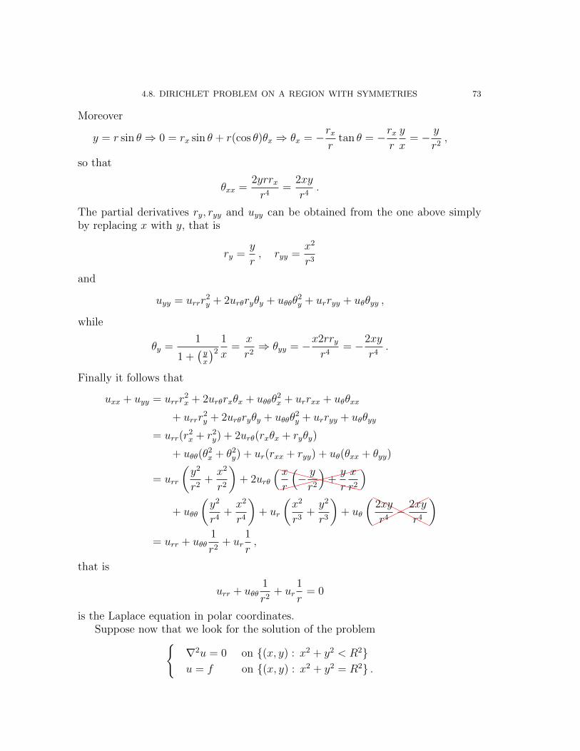
4.8. DIRICHLET PROBLEM ON A REGION WITH SYMMETRIES 73
Moreover
y = r sin θ ⇒ 0 = rx sin θ + r(cos θ)θx ⇒ θx = −rxr
tan θ = −rxr
y
x= − y
r2,
so that
θxx =2yrrxr4
=2xy
r4.
The partial derivatives ry, ryy and uyy can be obtained from the one above simplyby replacing x with y, that is
ry =y
r, ryy =
x2
r3
and
uyy = urrr2y + 2urθryθy + uθθθ
2y + urryy + uθθyy ,
while
θy =1
1 +(yx
)2
1
x=
x
r2⇒ θyy = −x2rry
r4= −2xy
r4.
Finally it follows that
uxx + uyy = urrr2x + 2urθrxθx + uθθθ
2x + urrxx + uθθxx
+ urrr2y + 2urθryθy + uθθθ
2y + urryy + uθθyy
= urr(r2x + r2
y) + 2urθ(rxθx + ryθy)
+ uθθ(θ2x + θ2
y) + ur(rxx + ryy) + uθ(θxx + θyy)
= urr
(y2
r2+x2
r2
)+ 2urθ
(���
������XXXXXXXXX
x
r
(− y
r2
)+y
r
x
r2
)+ uθθ
(y2
r4+x2
r4
)+ ur
(x2
r3+y2
r3
)+ uθ
(���
���HH
HHHH
2xy
r4− 2xy
r4
)= urr + uθθ
1
r2+ ur
1
r,
that is
urr + uθθ1
r2+ ur
1
r= 0
is the Laplace equation in polar coordinates.Suppose now that we look for the solution of the problem{
∇2u = 0 on {(x, y) : x2 + y2 < R2}u = f on {(x, y) : x2 + y2 = R2} .
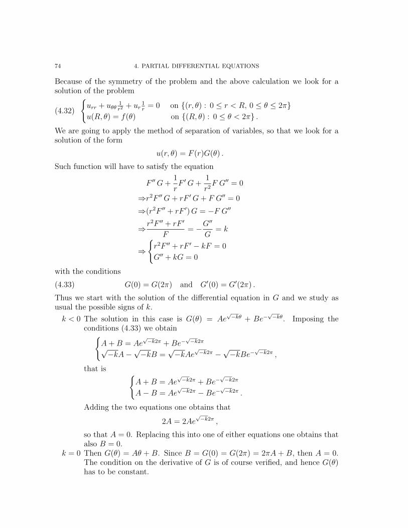
74 4. PARTIAL DIFFERENTIAL EQUATIONS
Because of the symmetry of the problem and the above calculation we look for asolution of the problem{
urr + uθθ1r2
+ ur1r
= 0 on {(r, θ) : 0 ≤ r < R, 0 ≤ θ ≤ 2π}u(R, θ) = f(θ) on {(R, θ) : 0 ≤ θ < 2π} .
(4.32)
We are going to apply the method of separation of variables, so that we look for asolution of the form
u(r, θ) = F (r)G(θ) .
Such function will have to satisfy the equation
F ′′G+1
rF ′G+
1
r2F G′′ = 0
⇒r2F ′′G+ rF ′G+ F G′′ = 0
⇒(r2F ′′ + rF ′)G = −F G′′
⇒r2F ′′ + rF ′
F= −G
′′
G= k
⇒
{r2F ′′ + rF ′ − kF = 0
G′′ + kG = 0
with the conditions
G(0) = G(2π) and G′(0) = G′(2π) .(4.33)
Thus we start with the solution of the differential equation in G and we study asusual the possible signs of k.
k < 0 The solution in this case is G(θ) = Ae√−kθ + Be−
√−kθ. Imposing the
conditions (4.33) we obtain{A+B = Ae
√−k2π +Be−
√−k2π
√−kA−
√−kB =
√−kAe
√−k2π −
√−kBe−
√−k2π ,
that is {A+B = Ae
√−k2π +Be−
√−k2π
A−B = Ae√−k2π −Be−
√−k2π .
Adding the two equations one obtains that
2A = 2Ae√−k2π ,
so that A = 0. Replacing this into one of either equations one obtains thatalso B = 0.
k = 0 Then G(θ) = Aθ + B. Since B = G(0) = G(2π) = 2πA + B, then A = 0.The condition on the derivative of G is of course verified, and hence G(θ)has to be constant.
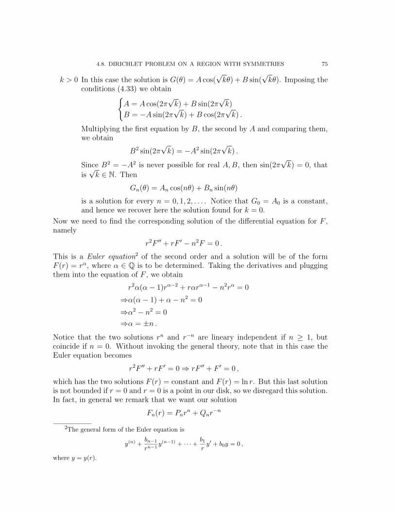
4.8. DIRICHLET PROBLEM ON A REGION WITH SYMMETRIES 75
k > 0 In this case the solution is G(θ) = A cos(√kθ) +B sin(
√kθ). Imposing the
conditions (4.33) we obtain{A = A cos(2π
√k) +B sin(2π
√k)
B = −A sin(2π√k) +B cos(2π
√k) .
Multiplying the first equation by B, the second by A and comparing them,we obtain
B2 sin(2π√k) = −A2 sin(2π
√k) .
Since B2 = −A2 is never possible for real A,B, then sin(2π√k) = 0, that
is√k ∈ N. Then
Gn(θ) = An cos(nθ) +Bn sin(nθ)
is a solution for every n = 0, 1, 2, . . . . Notice that G0 = A0 is a constant,and hence we recover here the solution found for k = 0.
Now we need to find the corresponding solution of the differential equation for F ,namely
r2F ′′ + rF ′ − n2F = 0 .
This is a Euler equation2 of the second order and a solution will be of the formF (r) = rα, where α ∈ Q is to be determined. Taking the derivatives and pluggingthem into the equation of F , we obtain
r2α(α− 1)rα−2 + rαrα−1 − n2rα = 0
⇒α(α− 1) + α− n2 = 0
⇒α2 − n2 = 0
⇒α = ±n .
Notice that the two solutions rn and r−n are lineary independent if n ≥ 1, butcoincide if n = 0. Without invoking the general theory, note that in this case theEuler equation becomes
r2F ′′ + rF ′ = 0⇒ rF ′′ + F ′ = 0 ,
which has the two solutions F (r) = constant and F (r) = ln r. But this last solutionis not bounded if r = 0 and r = 0 is a point in our disk, so we disregard this solution.In fact, in general we remark that we want our solution
Fn(r) = Pnrn +Qnr
−n
2The general form of the Euler equation is
y(n) +bn−1rn−1
y(n−1) + · · ·+ b1ry′ + b0y = 0 ,
where y = y(r).
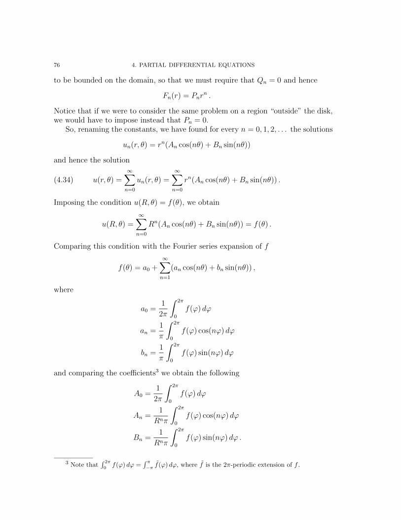
76 4. PARTIAL DIFFERENTIAL EQUATIONS
to be bounded on the domain, so that we must require that Qn = 0 and hence
Fn(r) = Pnrn .
Notice that if we were to consider the same problem on a region “outside” the disk,we would have to impose instead that Pn = 0.
So, renaming the constants, we have found for every n = 0, 1, 2, . . . the solutions
un(r, θ) = rn(An cos(nθ) +Bn sin(nθ))
and hence the solution
u(r, θ) =∞∑n=0
un(r, θ) =∞∑n=0
rn(An cos(nθ) +Bn sin(nθ)) .(4.34)
Imposing the condition u(R, θ) = f(θ), we obtain
u(R, θ) =∞∑n=0
Rn(An cos(nθ) +Bn sin(nθ)) = f(θ) .
Comparing this condition with the Fourier series expansion of f
f(θ) = a0 +∞∑n=1
(an cos(nθ) + bn sin(nθ)) ,
where
a0 =1
2π
∫ 2π
0
f(ϕ) dϕ
an =1
π
∫ 2π
0
f(ϕ) cos(nϕ) dϕ
bn =1
π
∫ 2π
0
f(ϕ) sin(nϕ) dϕ
and comparing the coefficients3 we obtain the following
A0 =1
2π
∫ 2π
0
f(ϕ) dϕ
An =1
Rnπ
∫ 2π
0
f(ϕ) cos(nϕ) dϕ
Bn =1
Rnπ
∫ 2π
0
f(ϕ) sin(nϕ) dϕ .
3 Note that∫ 2π
0f(ϕ) dϕ =
∫ π−π f(ϕ) dϕ, where f is the 2π-periodic extension of f .
4.8. DIRICHLET PROBLEM ON A REGION WITH SYMMETRIES 77
By replacing these coefficients into the equation (4.34), we obtain
u(r, θ) =1
2π
∫ 2π
0
f(ϕ) dϕ
+1
π
∞∑n=1
( rR
)n ∫ 2π
0
[cos(nθ) cos(nϕ) + sin(nθ) sin(nϕ)︸ ︷︷ ︸
cos(n(θ−ϕ))
]f(ϕ) dϕ
=1
2π
∫ 2π
0
f(ϕ) dϕ+1
π
∞∑n=1
( rR
)n ∫ 2π
0
cos(n(θ − ϕ))f(ϕ) dϕ .
Assuming we can exchange the series and the integral, we obtain
u(r, θ) =1
2π
∫ 2π
0
[1 + 2
∞∑n=1
( rR
)ncos(n(θ − ϕ))
]f(ϕ) dϕ .(4.35)
To manipulate the series, observe that if α ∈ R and for |t| < 1,
∞∑n=1
tn cos(nα) = <
(∞∑n=1
tneinα
)= <
(teiα
1− teiα
)= · · · = t cosα− t2
1− 2t cosα + t2,
so that
1 + 2∞∑n=1
tn cos(nα) =1− t2
1− 2t cosα + t2.
We use this identity with t = rR
and α = θ − ϕ and substitute the result in (4.35),so that
u(r, θ) =1
2π
∫ 2π
0
[1 + 2
∞∑n=1
( rR
)ncos(n(θ − ϕ))
]f(ϕ) dϕ
=1
2π
∫ 2π
0
1−(rR
)2
1− 2 rR
cos(θ − ϕ) +(rR
)2f(ϕ) dϕ
=1
2π
∫ 2π
0
R2 − r2
R2 − 2rR cos(θ − ϕ) + r2f(ϕ) dϕ .
The function
K(r, θ, R, ϕ) :=R2 − r2
R2 − 2rR cos(θ − ϕ) + r2
is called Poisson integral kernel and the solution
u(r, θ) =1
2π
∫ 2π
0
K(r, θ, R, ϕ)f(ϕ) dϕ
is given in Poisson integral form.
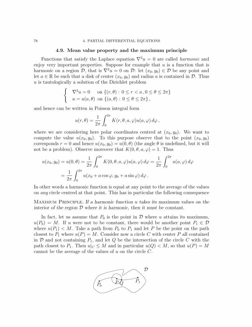
78 4. PARTIAL DIFFERENTIAL EQUATIONS
4.9. Mean value property and the maximum principle
Functions that satisfy the Laplace equation ∇2u = 0 are called harmonic andenjoy very important properties. Suppose for example that u is a function that isharmonic on a region D, that is ∇2u = 0 on D: let (x0, y0) ∈ D be any point andlet a ∈ R be such that a disk of center (x0, y0) and radius a is contained in D. Thusu is tautologically a solution of the Dirichlet problem{
∇2u = 0 on {(r, θ) : 0 ≤ r < a , 0 ≤ θ ≤ 2π}u = u(a, θ) on {(a, θ) : 0 ≤ θ ≤ 2π} ,
and hence can be written in Poisson integral form
u(r, θ) =1
2π
∫ 2π
0
K(r, θ, a, ϕ)u(a, ϕ) dϕ ,
where we are considering here polar coordinates centred at (x0, y0). We want tocompute the value u(x0, y0). To this purpose observe that to the point (x0, y0)corresponds r = 0 and hence u(x0, y0) = u(0, θ) (the angle θ is undefined, but it willnot be a problem). Observe moreover that K(0, θ, a, ϕ) = 1. Thus
u(x0, y0) = u(0, θ) =1
2π
∫ 2π
0
K(0, θ, a, ϕ)u(a, ϕ) dϕ =1
2π
∫ 2π
0
u(a, ϕ) dϕ
=1
2π
∫ 2π
0
u(x0 + a cosϕ, y0 + a sinϕ) dϕ .
In other words a harmonic function is equal at any point to the average of the valueson any circle centred at that point. This has in particular the following consequence
Maximum Principle. If a harmonic function u takes its maximum values on theinterior of the region D where it is harmonic, then it must be constant.
In fact, let us assume that P0 is the point in D where u attains its maximum,u(P0) = M . If u were not to be constant, there would be another point P1 ∈ Dwhere u(P1) < M . Take a path from P0 to P1 and let P be the point on the pathclosest to P1 where u(P ) = M . Consider now a circle C with center P all containedin D and not containing P1, and let Q be the intersection of the circle C with thepath closest to P1. Then u|C ≤ M and in particular u(Q) < M , so that u(P ) = Mcannot be the average of the values of u on the circle C.
P0P Q P1
D
4.10. WELL-POSED AND ILL-POSED PROBLEMS 79
4.10. Well-posed and ill-posed problems
Solutions of ordinary differential equations behave well, in the sense that, undercertain conditions, one can prove the existence and the uniqueness of the solutions ofan initial value problem, as well as the smooth dependence on the initial parameters.
The same statements unfortunately do not hold for partial differential equations,although the same questions arise. Not only we would like to know that a solutionof a given problem exist and is unique, but often the boundary conditions and theinitial conditions are obtained through measurements. So we would like to know thatthe solution is not affected too much by the likely imprecision with which boundaryconditions and initial conditions were measured.
We say that a problem is well-posed if it satifies the following three conditions:
(1) Existence: the problem has a solution;(2) Uniqueness: the solution is unique;(3) Stability: the solution depends continuously on the initial conditions and
on the boundary conditions.
The problem is ill-posed if one of the above properties does not hold. For partial dif-ferential equation there is no general theorem like in the case of ordinary differentialequations.
Example 4.16. We look for a solution of the differential equation
ux = c0u+ c1 ,
where u = u(x, y), c0 is a constant and c1 = c1(x, y). We are going to look atdifferent initial conditions, namely
(1) u(0, y) = f(y);(2) u(x, 0) = x in the case in which c1(x, y) = 0;(3) u(x, 0) = ec0x also in the case c1(x, y) = 0.
(1) Using the formula
y(x) = e−P (x)
(∫ x
0
eP (ξ)q(ξ) dξ + y(0)
)for the solution of a linear ordinary differential equation
y′ + p(x)y = q(x) ,
where
P (x) :=
∫ x
0
p(s)ds ,
we obtain
u(x, y) = ec0x(∫ x
0
e−c0ξc1(ξ, y) dξ + f(y)
),
where we used that u(0, y) = f(y). In this case the problem is well-posed.
80 4. PARTIAL DIFFERENTIAL EQUATIONS
(2) The differential equation is now
ux = c0u ,
so that
u(x, y) = g(y)ec0x ,
where g is a function to be determined with the initial conditions. Doing so, weobtain
x = u(x, 0) = g(0)ec0x
and hence
g(0) = xe−c0x .
But this is not possible since xe−c0x is not a constant, and hence the problem hasno solution.
(3) Like in (2) the solution is now
u(x, y) = g(y)ec0x ,
where g is a function to be determined with the initial conditions. Imposing theinitial conditions we obtain
ec0x = u(x, 0) = g(0)ec0x ,
from which it follows that any function g(y) with g(0) = 1 gives a different solution
u(x, y) = g(y)ec0x .
In this case the problem is not well-posed because the solution is not unique.
Example 4.17. It is easy to verify that the one-dimensional wave equation on aninfinite string is a well-posed problem for any initial conditions f, g. Recall in factthe problem
utt = c2uxx for t ≥ 0
u(x, 0) = f(x)
ut(x, 0) = g(x) ,
that has solution
u(x, t) =1
2
(f(x+ ct) + f(x− ct)
)+
1
2c
∫ x+ct
x−ctg(y) dy .
4.10. WELL-POSED AND ILL-POSED PROBLEMS 81
We want to investigate the change in u if f and g are replaced by f + δf and g+ δg.With the modified initial conditions the solutions becomes
uδ(x, t) =1
2(f(x− ct) + δf(x− ct) + f(x+ ct) + δf(x+ ct))
+1
2c
∫ x+ct
x−ct(g(y) + δg(y)) dy
= u(x, t) +1
2(δf(x− ct) + δf(x+ ct)) +
1
2c
∫ x+ct
x−ctδg(y) dy ,
so that
|u(x, t)− uδ(x, t)| ≤1
2
∣∣δf(x− ct) + δf(x+ ct)∣∣+
1
2cmax
∣∣δg(y)∣∣((x+ ct)− (x− ct)
)=
1
2δ∣∣f(x− ct) + f(x+ ct)
∣∣+ tmax∣∣δg(y)
∣∣ .If ε > 0, we can find a δ > 0 such that
1
2δ∣∣f(x− ct) + f(x+ ct)
∣∣ < ε and max δ∣∣g(y)
∣∣ < ε ,
from which it follows that
|u(x, t)− uδ(x, t)| < ε+ tε .
It should be noted that, although this shows continuity on the initial parameter, wealso see the the more time goes by, the more the function uδ differs from u.
Example 4.18. The Neumann problem on a region R is the following{∇2u = 0 on R∂u∂n
= g on ∂R .
We see now that a necessary condition for the existence of a solution is that∫∂Rg = 0.
In fact, using the divergence theorem, we obtain∫∂R
g =
∫∂R
∂u
∂n=
∫∂R
∇u · n =
∫R
div(∇u) dA =
∫R
∇2u = 0 ,
which shows that the Neumann problem is not well-posed if∫∂Rg 6= 0.