AD-A276 593

DOT/FAAICT-3I77DOT-VNTSC-FAA.AC3-7

FAA Tecnical .o Analysis Concening theAtlantic Cky IntunatOna AiqrpodN.J. 06405

......... ?::,<:•...

December 1993

Final Report

This1.,cr7T -- EM ',AR 0 2 1994

Thl publicthrough the nical informationService, Springfield, Virginia 22161.

OU.S. Doemont of TwaportationFederal Aviston Administraton

S94094-06780I I lllllililll 0? I0 9 3

NOTICE

This document is disseminated under the sponsorship of theDepartment of Transportation in the interest of informationexchange. The United States Government assumes no liability forits contents or use thereof.

NOTICE

The United States Government does not endorse products ormanufacturers. Trade or manufacturers' names appear hereinsolely because they are considered essential to the objective of thisreport.

REPORT DOCUMENTATION PAGE 1PyLI[ Ourriy burden 9fo nlr this coltec Ion informt tlon fi ftltmtsd to ever"" I per urdn uotbe

1. AENCY• OLY (oev bta) 2 REPRT ATE . REPORT TYPE Mi DATES CO•ItED

ft evlnoIe i@boseorcs gathrin Final Report

[April 1991 - June 1991

I.. TITLE AND SUTITLE 5. FUNDING NWUNERSAnalysis Concerning the Inspection Threshold for Multi-Site

DamageFA3H3/A31286. AUTHOR(S) DTRS57 -91-P-80859David Broek

7. PERFORMING ORGANIIZATION NAME(S) AND ADORESS(ES) 8. PERFORMNilG ORGANIZATIONFractureREsearch, Inc. * REPORT KUNBER9049 Cupstone DriveDT-TSFA-97Galena, OH 43021

9. SPONSORING/MONITORING AGENCY NAME(S) AND ADDRESS(ES) 10. SPONSORING/MONITORNIIGU.S. Department of Transportation AGENCY REPORT MISJNEIFederal Aviation Administration Technical CenterEngineering, Research, and Development •ervice DOT/FAA/CT-93/77Atlantic City International Airport, NJ 08405

11. SUPPLEMENTARY NOTES U.S. Department of Transportstion' wnder contract to: Research and Special Progra Administration

Vofpe National Tranportation Systems CenterCaidsridge,_MA__02142-1093______________

12a. DISTRIAUTIONLAVAILABILITY STATEMENT 12b. DISTRIBUTION CORD

This document is available to the public through the NationalTechnical Information Service, Springfield, VA 22161

13. ABSTRACT HANLm uL 200 words)

Periodic inspections, at a prescribed interval, for Multi-Site Damage (MSD) inlongitudinal fuselage lap-joints start when the aircraft has accumulated a certainnumber of flights, the inspection threshold. The work reported here was an attempt toobtain justification for the threshold. It is based upon an analysis of fatigue datafor lap-joints (riveted as well as riveted plus bonded) of a configuration closelyresembling those in several types of aircraft. Depending upon the definition ofthreshold, the results show that it will be around 30,000 flights. Graphs aresupplied upon the basis of which airworthiness authorities can determine a thresholdin accordance with their preferred definition, and for different service conditions.

14. SUBJECT TERMS 15. HNUNSER OF PAGESMulti-Site Damage (HSD), fuselage, lap-joints, threshold

16. PRICE CODE

17. SECURITY CLASSIFICATION 18. SECURITY CLASATION TION 19. SEUITSLSCTION 20. LIMITATION OF ABSTRACTOF REPORT OF THIS PAGE OF ABSTRACTUnclassified Unclassified Unclassified

NSN 7540-01-280-5500 Standard Form 298 (Rev. 2-89)Prescribed by ANSI Std. 239-18298-102

1 SUPEETR NOTE U.S Deatmn of ITransporiation

Periodic inspections, at a prescribed interval, for Multi-SiteDamage (MSD) in longitudinal fuselage lap-joints start when theaircraft has accumulated a certain number of flights, the inspec-tion threshold. The work reported here was an attempt to obtainjustification for the threshold. It is based upon an analysis offatigue data for lap-joints (riveted as well as riveted plusbonded) of a configuration closely resembling those in severaltypes of aircraft. Depending upon the definition of threshold, theresults show that it will be around 30,000 flights. Graphs aresupplied upon the basis of which airworthiness authorities candetermine a threshold in accordance with their preferred defini-tion, and for different service conditions.

This report was prepared for the Volpe National TransportationSystems Center in support of the Federal Aviation AdministrationTechnical Center under contract DTRS57-91-P-80859.

Accesion For

U ...............

ii Codes

A 'il ai~ lIor

Dit iiCj

NETRIC/ENGLISN CONVERSION FACTORS

ENGLISH TO METRIC METRIC TO ENGLISH

LENGTH (APPROXIMATE) LENGTH (APPROXIMATE)

I Inch (in) a 2.5 centimeters (cm) 1 millimeter (m) a 0.04 Inch (in)

1 foot (ft) - 30 centimeters (cm) 1 centimeter (cm) a 0.4 Inch (in)

1 yard (yd) a 0.9 meter (a) 1 meter (m) a 3.3 feet (ft)

1 oiLf (ol) a 1.6 kilometers (kin) 1 meter (s) a 1.1 yards (yd)

1 kitlometer (In) a 0.6 iteL (ml)

AREA (APPROXIMATE) AREA (APPROXIMATE)

1 square Inch (sq in, in2 a 6.5 sqare centimeters (cm2 ) I square centimeter (cm2 ) a 0.16 square inch (sq in, In 2 )

1 square foot (sq ft, ft 2 - 0.09 square meter (m) 1 sqare meter (62) a 1.2 sqare yearde (sq yd, yd2 )

1 sqare yard (sq yd, yd2 ) a 0.8 square meter (m2 ) 1 square kiLometer (k-2) . 0.4 square mite (sq mo, mi 2 )

1 square mile (sq oi, fl 2) a 2.6 square kilometers (km2) I hectare (he) a 10,000 square meters (m2) a 2.5 acres

1 acre a 0.4 hectares (he) a 4,000 square meters (.2)

MASS - IWEIGHT (APPROXIMATE) MASS - WEIGHT (APPROXIMATE)

I ounce (oz) w 28 grams (gr) 1 grew (or) a 0.036 ounce (oz)

I pound (0b) w .45 kilogram (kg) 1 ki!ogron (kg) a 2.2 pounds (0b)

1 short ton - 2,000 pounds (tb) a 0.9 tonne (t) I tonne Mt) a 1,000 kilogram (kg) a 1.1 short taos

VOLUME (APPROXIMATE) VOLUME (APPROXIMATE)

1 teaspoon (tsp) x 5 milliliters (mL) 1 milliliters (mL) a 0.03 fluid ounce (ft oz)

1 tablespoon (tbsp) a 15 milliliters (mt) I liter (1) a 2.1 pints (pt)

1 fluid ounce (ft oz) z 30 milliliters (ml) 1 liter (1) - 1.06 quarts (qt)

1 cup (c) - 0.24 liter (1) 1 liter (1) a 0.26 gallon (gat)

1 pint (pt) a 0.47 liter (1) 1 cubic meter (m3) - 36 cubic feet (cu ft, ft 3 )

1 quart (qt) x 0.96 liter (1) 1 cubic meter (W3) - 1.3 cubic yards (cu yd, yd3 )

1 gallon (gat) a 3.8 liters (1)

1 cubic foot (cu ft, ft 3 ) - 0.03 cubic meter (m3)

1 cubic yard (cu yd, yd3 ) - 0.76 cubic meter (i3)

TEMPERATURE (EXACT) TE1MPERATURE (EXACT)

[(x-32)C5/9)] 0 F y OC C(9/5) y + 321 °C a x OF

WUICK INCH-CENTIMETER LENGTH CONVERSION

INCHES 0 1 2 3 4 5 6 7 8 9 10I- I I I I I I I

CENTIMETERS 0 1 2 3 4 5 6 7 8 9 10 11 12 13 14 15 16 17 18 19 20 21 22 23 24 25125.40

QUICK FAHRENHEIT-CELSIUS TEMPERATURE CONVERSION

OF .400 .220 .40 140 320 50o 680 860 1040 1220 1400 1580 1760 19940 21200a I5 0 I I I IIooo

Occ -460 -30 26 0 04~j~ 6~0 160 200 360 460~ 56 66 6I6 900 16000

For more exact and or other conversion factors, see NBS Miscellaneous Publication 286, Units o Weights andMeasures. Price $2.50. SD Catalog No. C13 10286.

iv

TABLE OF COITENTS

Section a

1. INTRODUCTION AND SCOPE .................. 1

2. AVAILABLE DATA .*. . . . * . * . * . . *. . . 2

2.1 Description of Database...... . . . . . . . . .22.2 Scatter and Distribution Function . . . . . . . . . . 3

3. DISTRIBUTION OF INITIATION LIFE IN PRACTICE . . . . . . . 5

3.1 Estimate of Applicable S-N Curve . . . . . . . . . . 53.2 Calculation of Initiation and Scatter . . . . . . . . 7

4. CONSIDERATIONS FOR THRESHOLD . . . . . . . . . . . . . . 10

4.1 Definition of Threshold...... . . . . . . . . 104.2 Resulting Flight Numbers Till Threshold . . . . . . 114.3 The Crack Growth Approach. . . . . . . . . . . . . 11

5. CONCLUSION . . . . . . . . . . . . . . . . . . . . . . . 13

6. REFERENCES . . . . . . * . . . . . . . . . . . 14

v

zigaLIST OF VXGMUILU

1. TESTS BY HARTHNW . . .. . . . . ......... 15

2. ALL DATA FOR FAILURES IN ADHESIVE; NOTAT HOLES - ALL CONDITIONS (HARTMAN DATAFOR RIVETED PLUS BONDED LAP-JOINTS) . . . . . . . 16

3. ALL DATA FOR FAILURES AT HOLES (HARTMANDATA FOR RIVETED AND BONDED LAP-JOINTS;HARTMAN DATA) . . . . . . . . . . . . . * 0 17

4. HARTMAN DATA FOR LAP-JOINTS RIVETED PLUSBONDED AND RIVETED ONLY (CONSOLIDATION OFALL HARTMAN DATA) . . . . . . . . . . . . . 18

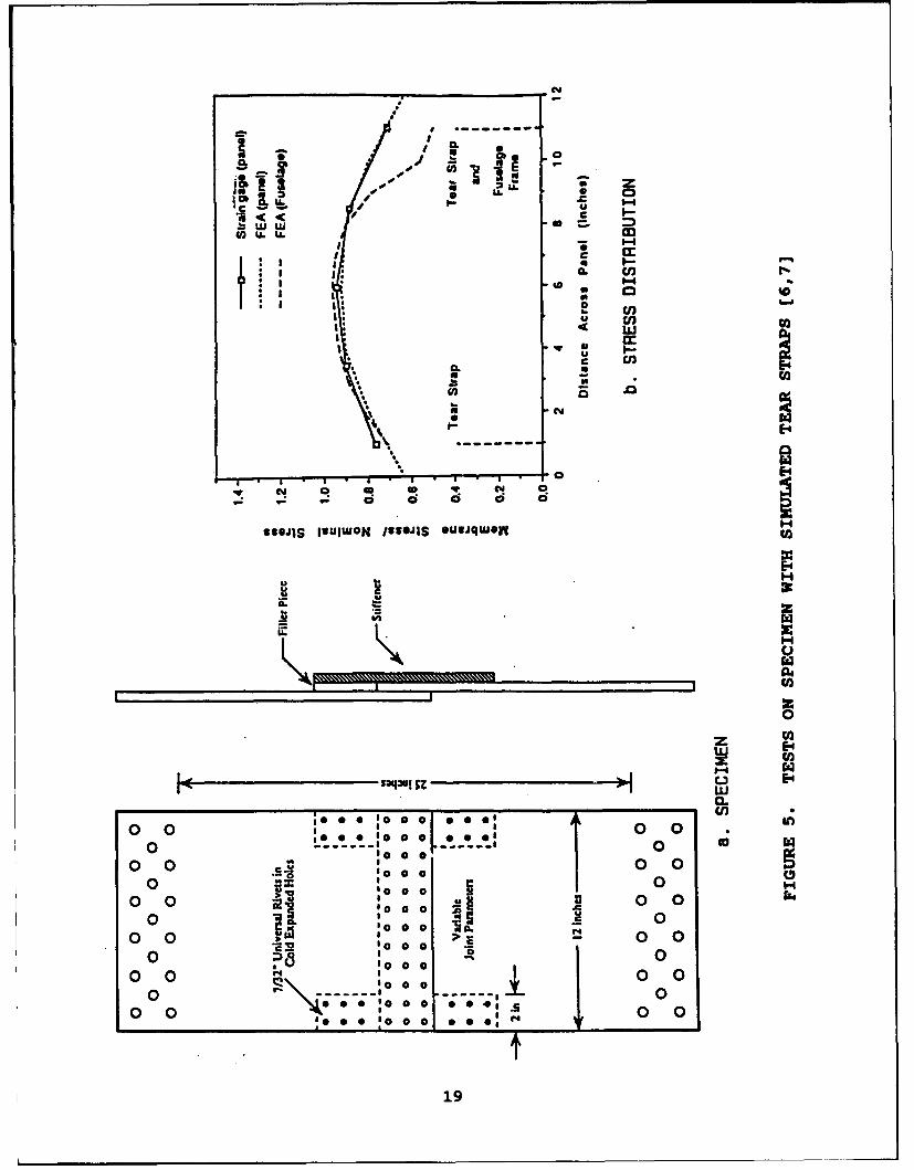
5. TESTS ON SPECIMEN WITH SIMULATED TEARSTRAPS [6,7] . . . . . . . . . . . . . . . . . . 19

6. COMPARISON OF MEAN S-N CURVES . . . . . . . . . . 20

7. HOLE-FAILURES AT HIGH AND LOW FREQUENCY -ADHESIVE AND NON-AGED (HARTMAN DATA FORRIVETED PLUS BONDED LAP-JOINTS) . . . .... .. 21

8. DATA FOR ALL HOLE FAILURES: HIGH AND LOWFREQUENCY - ADHESIVE AGED AND NON-AGED(HARTMAN DATA FOR RIVETED PLUS BONDED) . . . . . 22

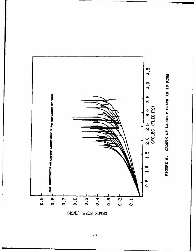
9. GROWTH OF LARGEST CRACK IN 10 RUNS . . . . . . . 23

10. MEASURED CRACK GROWTH CURVES [6,7] . . . . . . . 24

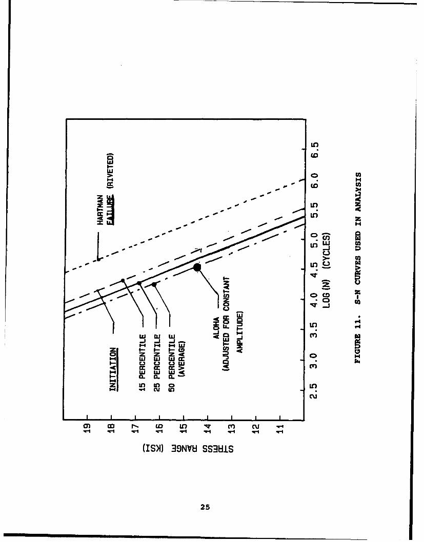
ii. S-N CURVES USED IN ANALYSIS. . . . . . . . . . . 25

12. OPTIMISTIC CASE WHERE ALOHA BELONGS TOLOWER 15 PERCENTILE .............. 26

13. CASE IN WHICH ALOHA BELONGS TO LOWER 25PERCENTILE . . . . . . . . . . . . . . o . . . . 27

14. CONSERVATIVE CASE WHERE ALOHA IS AVERAGE . . . . 28

15. THREE CASES FOR DIFFERENTIAL PRESSURE OF8 psi . . . . . . . . . . . . . . . . . . . . . . 29

16. FINAL CRACK SIZES AT ALL LOCATIONS - SAMECASE AS IN FOLLOWING - SOLID LINE: LEFTCRACK; DASH-DOT; RIGHT CRACK . . . . . . . . . . 30

vi

LIST OF FXGU138 (continued)

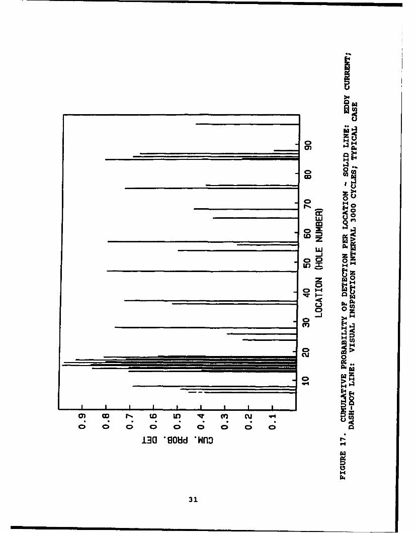
17. CUMULATIVE PROBABILITY OF DETECTION PERLOCATION - SOLID LINE: EDDY CURRENT;DASH-DOT LINE: VISUAL INSPECTION INTERVAL3000 CYCLES; TYPICAL CASE . . . . . . .... . 31

18. MEASURED CRACK SIZES AT FAILURE [6,7] . . . . . . 32

19. SIZES OF DETECTED MSD IN AIRCRAFT [6,7] . . . . . 33

20. SIZE DISTRIBUTION WHEN LARGEST CRACK IS0.1 INCH . . . . . . . . . .. *. . . . . . . . .. 34

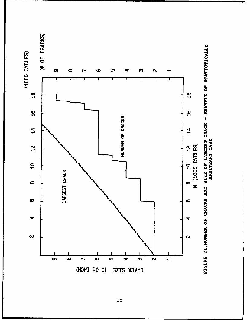
21. NUMBER OF CRACKS AND SIZE OF LARGESTCRACK - EXAMPLE OF STATICALLY ARBITRARY CASE 35

22. SIZE DISTRIBUTION WHEN LARGEST CRACK IS0.1 INCH . .. .. .. .. .. .. .. .. . .. 36

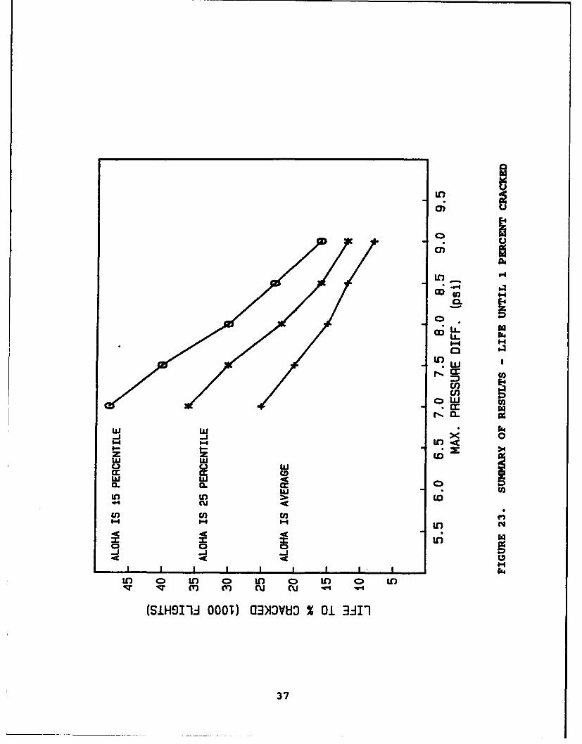
23. SUMMARY OF RESULTS - LIFE UNTIL 1 PERCENTCRACKED . . .. . . . ... . . . . . . 37

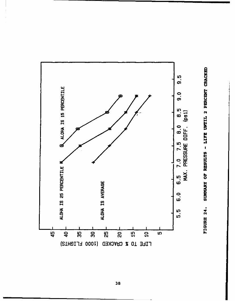
24. SUMMARY OF RESULTS - LIFE UNTIL 2 PERCENTCRACKED . . . . . . . . . . . . . . . . . . . . 38

25. SUMMARY OF RESULTS - LIFE UNTIL 5 PERCENTCRACKED . . . . .. . . . . . . . . . . . . . 39

26. SUMMARY OF RESULTS - CASE WHERE ALOHABELONGS TO LOWER 25 PERCENTILE . . . . . . . .. 40

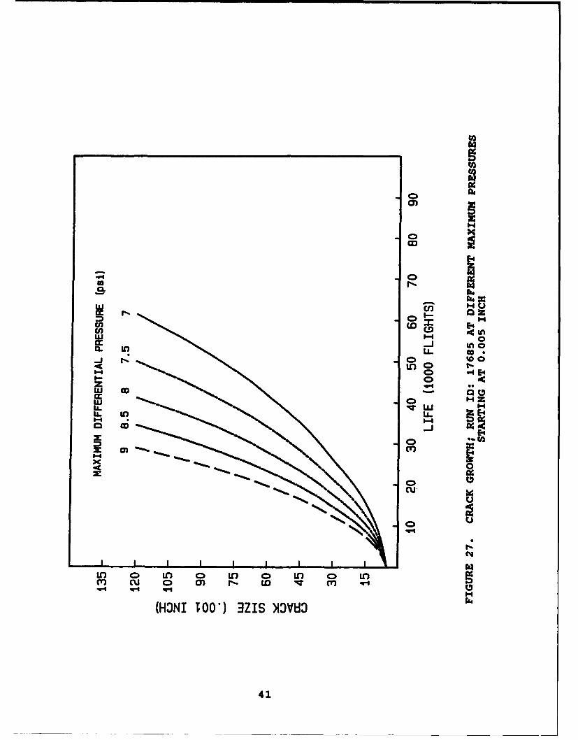
27. CRACK GROWTH; RUN ID: 17685 AT DIFFERENTMAXIMUM PRESSURES STARTING AT 0.005 INCH . . . . 41

28. LIFE UNTIL 0.12 INCH CRACK AS A FUNCTION OFASSUMED EQUIVALENT INITIAL FLAW (EIF) SIZE . . . 42

vii/viii

1. INTRODUCTION AND SCOPE

The cumulative probability of detection of Multi-Site Damage (MSD)in fuselage lap-joints of aging aircraft was assessed in a previousstudy [1]. It showed that inspection intervals on the order of 3000to 4000 flights provide cumulative probabilities of detection onthe order of 0.98 (98 percent detected) or better if inspectionsare performed by eddy current. Although quite a few assumptionswere necessary, a sensitivety analysis showed the effect of theassumptions to be small.

It is unlikely for MSD to occur very early in life, becausedisbonding of the adhesive will take some time. Therefore, andbecause the probability of detection is virtually zero in the earlystages of MSD, it is un-economical to adhere to the prescribedinspection interval from time zero. Hence an inspection thresholdwas instituted by stipulating that inspections for MSD need notstart until after the accumulation of a certain number of flights.The present study was undertaken to provide a justification forthis threshold.

As the alotted time for this work was very limited, only readilyavailable results of fatigue tests on lap-joints were analyzed. Thetest data were used primarily to obtain the scatter (i.e.distribution function) for the start of cracking: the scatterdetermines when the earliest detectable MSD may occur. The onlytrue service experience comes from the Aloha incident. The time tofailure for the latter case was used as the anchor point for theestimate of the fatigue-life curves (S-N curves) for serviceconditions. As this approach needed only a few reasonableassumptions, it is considered to provide a realistic assessment ofthe threshold.

Another procedure to determine inspection thresholds is based uponcrack growth analysis. It is then assumed that a certain crack isalready present in the new structure, and the time it takes forthis initial crack to grow to a "detectable" size, is used for theinspection threshold, either directly or with a safety factor. Thisprocedure has found some acceptance by the industry and by FAAcertification offices. The initial "crack" is not a real crack butrather an Equivalent Initial Flaw (EIF), where the qualifier"equivalent" indicates that if the EIF is used in analysis, it willlead to acceptable results. Unfortunately, the results dependstrongly upon the assumed size of the EIF, while the commonly usedvalue of 0.05 inch cannot very well be justified. Nevertheless,this approach was used in the present work as well to obtain acomparison with the analysis based upon fatigue life. The resultsare of the same order of magnitude as those based upon lifeanalysis.

2. AV.LrL.UIU DALTA

2.1 DICtIP•TION 0F D&TA S3UN

Readily available fatigue test data for joints were those inReferences 2 through 8. A diligent search of older reports(1950-1965) by NACA (NASA), RAE, NLR, FFA, ARL, and so on, islikely to provide a wealth of additional data, but timeconstraints did not permit such a search and associated dataanalysis. Of the sources readily available some were for conditionsand configurations not immediately relevant to the problem at hand,but the large data base generated by Hartman (2] is veryappropriate, as are a few data generated recently [6,7].

It should be noted that in all of the following the stresses arethe nominal stresses away from the joint: they represent the hoopstress in a fuselage. This simulated hoop stress is not necessarilyequal to that due to presurization, as will be explained later.Furthermore, all data are for a stress ratio, R, of 0.05 to 0.1,while fuselage loading is essentially at R = 0. As a consequence,the assumption had to made that the results are applicable to theslightly different fuselage loading, but this of minor importancebecause the effect of the associated difference in mean stress issmall.

Hartman's data [2] are especially useful, because they wereobtained from tests on adhesively bonded and riveted lap-joints ofa configuration (Figure 1) almost identical to the one used in thefuselage of several types of aircraft. Hartman performed well over400 tests. The lap-joints specimens were bonded with a cold-curingadhesive, and contained 3 rows of countersunk fasteners. Hartmaninvestigated the effect of many parameters, the most important ofwhich are: (1) Two adhesives, namely AWl06 (CIBA) and EC226 (3M);(2) two types of surface treatment, namely chromic acid andsulphuric acid anodizing; (3) Three testing temperatures, namely-55C (stratosphere), 20C and 50C (aircraft taking of after exposureto summer sun at airport); (4) in one series of tests the adhesivewas intentionally maltreated by exposure to 100% RH at70C for 4weeks; (5) three loading frequencies, nimely 6, 240 and 3000 cpm;(6) several different stress levels.

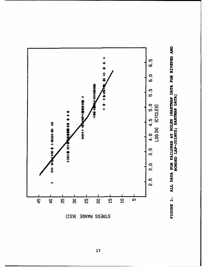
Part of the specimens failed at the adhesive fillet or elsewhereaway from the fastener holes. These data, regardless of testparameter, are shown in Figure 2. As MSD occurs at the fastenerholes, these data were excluded from the following analysis. Wellover 200 of Hartman's specimens failed at the fastener holes. Theyare shown in Figure 3, again regardless of test parameters. Hartmandid a limited number of tests on specimens that were riveted only(as opposed to riveted and bonded). The data of these tests areshown in Figure 4. Also shown in Figure 4 are the data pointsobtained at low frequency loading (which is the most relevant forlongitudinal fuselage joints) for riveted plus bonded joints whichfailed at the holes.

2

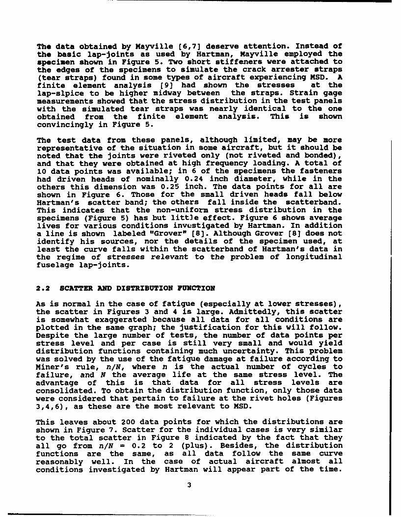
The data obtained by Mayville (6,7] deserve attention. Instead ofthe basic lap-joints as used by Hartman, Mayville employed thespecimen shown in Figure 5. Two short stiffeners were attached tothe edges of the specimens to simulate the crack arrester straps(tear straps) found in some types of aircraft experiencing MSD. Afinite element analysis [9] had shown the stresses at thelap-slpice to be higher midway between the straps. Strain gagemeasurements showed that the stress distribution in the test panelswith the simulated tear straps was nearly identical to the oneobtained from the finite element analysis. This is shownconvincingly in Figure 5.

The test data from these panels, although limited, may be morerepresentative of the situation in some aircraft, but it should benoted that the joints were riveted only (not riveted and bonded),and that they were obtained at high frequency loading. A total of10 data points was available; in 6 of the specimens the fastenershad driven heads of nominally 0.24 inch diameter, while in theothers this dimension was 0.25 inch. The data points for all areshown in Figure 6. Those for the small driven heads fall belowHartman's scatter band; the others fall inside the scatterband.This indicates that the non-uniform stress distribution in thespecimens (Figure 5) has but little effect. Figure 6 shows averagelives for various conditions investigated by Hartman. In additiona line is shown labeled "Grover" [8]. Although Grover [8] does notidentify his sources, nor the details of the specimen used, atleast the curve falls within the scatterband of Hartman's data inthe regime of stresses relevant to the problem of longitudinalfuselage lap-joints.

2.2 SCATTER AND DISTRIBUTION FUNCTION

As is normal in the case of fatigue (especially at lower stresses),the scatter in Figures 3 and 4 is large. Admittedly, this scatteris somewhat exaggerated because all data for all conditions areplotted in the same graph; the justification for this will follow.Despite the large number of tests, the number of data points perstress level and per case is still very small and would yielddistribution functions containing much uncertainty. This problemwas solved by the use of the fatigue damage at failure according toMiner's rule, n/N, where n is the actual number of cycles tofailure, and N the average life at the same stress level. Theadvantage of this is that data for all stress levels areconsolidated. To obtain the distribution function, only those datawere considered that pertain to failure at the rivet holes (Figures3,4,6), as these are the most relevant to MSD.

This leaves about 200 data points for which the distributions areshown in Figure 7. Scatter for the individual cases is very similarto the total scatter in Figure 8 indicated by the fact that theyall go from n/N = 0.2 to 2 (plus). Besides, the distributionfunctions are the same, as all data follow the same curvereasonably well. In the case of actual aircraft almost allconditions investigated by Hartman will appear part of the time.

3

Therefore all data were considered to belong to one populationcovering all service conditions for aircraft. This leads to thedistribution function shown in Figure 8. Not only is this generaldistribution function the same as the one for the individual casesin Figure 7, it turns out that the data fit the Weibul distributionvery well.

Mi-sr's rule predicts crack inititation if Sum n/N - 1. The datashow that due the scatter, failure occurs at values between 0.15and 2. The Weibul parameters in Figure 8 were more or lessconfirmed by other data [3,4,5]. The distribution function is:

Pf - 1 - exp(- (n/N - Do)/(A - Do)- x)

where Pf is the fraction (percentage) failed, or probability offailure, while Do, A, and X are the shape parameters the values ofwhich are shown in Figures 7 and 8. The average (Pf = 0.5) isindeed at n/N - 1.

4

3. DZBTRXBUTXON OF INXTIATZON LIVE IN PRACTICZ

3.1 3TIXXR!TE OF APPLICABLE S-N CURVE

Although the above provides the distribution of n/N, the actualaverage life, N, under aircraft service conditions is not known.However, one important actual service data-point is available fromthe Aloha incident: the failure occured at 89600 flights.Accounting for the fact that the average time for crack growth tofailure is 25,000 flights the initiation time is estimated at64,000 flights.

The average of 25,000 flight cycles for crack propagation followsfrom previous work [10] in which crack growth was calculated for avariety of statistical parameters (assigned by a Monto-Carlotechnique) and for a variety of circumstances. An example of thesecomputations is shown in Figure 9. The number is confirmed by dataobtained by Mayville [6,7] shown in Figure 10. Although the crackgrowth curves in Figure 10 start at different cycle numbers, theyare well-nigh parallel. The total growth from initiation to failurecovers about 20,000 to 25,000 cycles, if initiation is consideredas the appearance of a crack of about 0.02 inch size. From apractical point of view this is a good definition, because at 0.02inch the crack will just emerge from under the fastener head andbecome inspectable.

The remaining question is then where the Aloha case falls in thescatter band, i.e. whether the case is an extreme. One might arguethat it is, because Aloha operates in adverse conditions (lowaltitude flights over sea). But MSD was detected in many otheraircraft as well, indicating that Aloha was not an extreme. Threecases were considered, namely:

1. Aloha is average (or 50 percentile; conservative).2 Aloha belongs to the lower 25 percentile3. Aloha belongs to lower 15 percentile (optimistic; it is

an extreme).

For each of these percentiles the value of n/N can be read fromFigure 8, from which the average life N can be found. Making thereasonable assumption that all S-N curves have the same slope, thelife-to-initiation curves for the above 3 conditions, and for thestress levels encountered in service can be determined to be asshown in Figure 11, and as explained below.

For the relevant stress ranges in the regime of 10 to 20 ksi the S-N curve can be represented by a straight line on semi-logarithmicscales, and hence by the equation:

S= A-q lnN

5

which can be inverted to:

N - exp ((A - S) /q)

where N is the life to crack initiation, S the stress range, and Aand q are parameters. That all lines should be parallel (sameslope) in the region of interest can be ascertained from Figures 3,4, and 6; this results in a fixed value for q of 2.74. (Althoughthe data in the previous figures were plotted, in accordance withengineering practice, on 10-log scale, the natural logarithm wasused in the equations.) Hence, the difference in the lines shown inFigure 11 is characterized by different values of A.

As flights are of different length the cruising altitude (and hencethe differential pressure) varies from flight to flight. This meansthat the loading is not of constant amplitude. Since the S-N curveswere to be "anchored" on the Aloha case, the Aloha experienceservice experience is detailed below:

Altitude Delta-p % of flights Pressure relative to highest(ft) (psi)

>18000 7.5 23 1.0016000 6.7 5 0.89

<14000 6.1 72 0.81

According to the finite element analysis [9] the membrane stress atmid-bay is 14.9 ksi, but this number is for a skin thickness of0.04 inch and a differential pressure of 8.5 psi. In the actualaircraft the maximum pressure was 7.5 psi (above table), bringingthe maximum operating stress to 14.9 * 7.5/8.5 = 13.15 ksi. Due tothe lower skin thickness another 10 percent must be added, whichprovides a maximum stress of 14.5 ksi.

If the Aloha case was the average (50 %) crack inititiation, asdefined above, occurred at n/N = 1, at 64,000 cycles as explained.The table shows that the highest stress of 14.5 ksi occurred in 23percent of the flights, i.e. in 0.23 * 64,000 = 14,720 flights.

The membrane stress in the other flights at differential pressuresof 6.7 and 6.1 psi are obtained as 14.5*6.7/7.5 = 13 ksi, and 14.5* 6.1/7.5 = 11.8 ksi, respectively. The associated cycle numbersare 0.05 * 64,000 = 3,200, and 0.72 * 64,000 = 46,000,respectively.

With this information a system of 4 equations with 4 unknowns canbe solved to obtain A. The result is A = 43, so that the equationfor the life becomes:

N = exp((43 - S)12.74)

6

The membrane stress in the other flights at differential pressuresof 6.7 and 6.1 psi are obtained as 14.5*6.7/7.5 - 13 ksi, and 14.5* 6.1/7.5 - 11.8 ksi, respectively. The associated cycle numbersare 0.05 * 64,000 - 3,200, and 0.72 * 64,000 - 46,000,respectively.

With this information a system of 4 equations with 4 unknowns canbe solved to obtain A. The result is A - 43, so that the equationfor the life becomes:

N = exp((43 - S)/2.74)

Inverting this procedure permits calculation of sum n/N for thiscase as follows:

S (ksi) n N (for A = 43) n/N

14.5 14,720 32,900 0.44713.0 3,200 56,900 0.05611.8 46,000 88,200 0.522

Sum n/N 1.025

Hence, if Aloha is an average case, the S-N curve with A = 43,shown in Figure 11, is the applicable curve for the average life toinitiation. For the other cases defined above a similar procedureleads to the average S-N curve. However, it can be seen immediatelywhat the results will be, because all calculations are based uponproportionality. Figure 6 shows that for a probability ofinitiation of 25 percent the value of n/N = 0.70, while for aprobability of 15 percent it is 0.52. Thus it can be deducedimmediately that the associated lives for all stresses are higherby a factor of 1/0.70 = 1.43, and 1/0.52 = 1.92 respectively,leading to values for A of 44 and 44.8 respectively; these arerepresented by the other lines in Figure 11.

Although superfluous, it should be pointed out that for thefollowing computations the lines in Figure 11 should beinterpreted as averages. For example, if the line for A = 43 is theaverage, the Aloha case will be average (as signified by the Alohacase falling on this line); but if the line for A = 44 is theaverage, the Aloha case falls left of the line, as shown in Figure11. The curves in Figure 11 pertain to the average life N. Tothis the scatter (distribution function) of Figure 8 was applied.

3.2. CALCULATION OF INITIATION LIFE AND SCATTER

The S-N curve(s) and distribution function now being known, thelife to initiation can be calculated. To this end a small computerprogram was developed. The program employs the membrane stresses

7

across a bay as calculated by the finite element analysis (9] fora pressure differential of 8.5 psi (Figure 5), as shown below:

11.1 ksi (at frame and straps) at 10% of holes12.6 ksi at 20% of holes13.8 ksi at 20% of holes14.5 ksi at 20% of holes14.8 ksi at 20% of holes14.9 ksi (midbay) at 10% of holes

The nominal membrane stress was used in the analysis, because alldata previously discussed are in terms of this nominal stress. Thenominal stress for any pressure differential the can be obtainedby multiplying the above stresses by p/8.5.

Many airlines service longer routes than Aloha, so that theirmaximum pressure (altitude) will be higher. It seems reasonablehowever, lacking data from other airlines, to assume that the lasttwo columns in the Aloha usage table provide an appropriateestimate of "general" usage relative to maximum pressuredifferential. Therefore, the calculations were based upon a usagespectrum in accordance with the one shown for Aloha, relative to amaximum operating pressure of 1, and Miner's rule for theaccumulation of damage at the three stress ranges (differentialpressures). The maximum operating pressure differential is thenthe only variable, because the other pressures are given relativeto the maximum. It permits computation of the membrane stresses atthe holes according to the conversion rule discussed, andsubsequently, assessment of the damage, Sum n/N, according to thegeneralized usage spectrum.

Apart from being directly dependent upon fuselage pressurization,the membrane stress depends upon aerodynamic pressure. Theaerodynamic pressure varies from point-to-point due to the fuselageshape, but should be assessed at about 0.5 psi on average [12] .This will increase the pressure differential locally, and hence,the membrane stresses will be higher than those following fromfuselage pressurization. This may explain why MSD appears to bemore prevalent at joints in the fuselage crown just behind theflight deck. Another area where this effect is significant is thevicinity of the wing-fuselage connection.

If the pressure differential by fuselage pressurization is forexample 8 psi, the actual local pressure differential would be onthe order of 8.5 psi, and possibly higher close to the wing-fuselage connection. The above was invoked in the small computerprogram already mentioned.

Accounting for all the effects discussed above calculations weremade of the per cent failed (holes cracked). The computations werecintinued until 10 percent of the holes were cracked, for thecases discussed and for different pressures. The results of thecomputations are shown in Figures 12 through 14 for variouspressure differentials (as adjusted for usage spectrum and local

8

aerodynamic pressure), and for cases where the Aloha case is thelower 15, 25 and 50 percentile. For a particular maximum pressuredifferential of 8 psi (accounting for an aerodynamic differentialof 0.5 psi), the results are shown in Figure 15. Similar crossplots can be made for other pressures by using the data in Figures12 through 14. The results are trivial in a way, because theymerely restate the lower end of the distribution function for aparticular set of circumstances.

9

4. CONSXDZDATXONS O= THRESHOLD

4.1. DZIN'ZTON TOFTHTESZHOLD

A more specific definition of threshold is now needed. In essencethe threshold is the time at which inspections must be started.There is no use for inspections as long as the cracks cannot befound, i.e. if they are so small that the probability of detectionis virtually zero. From execution of the computer program for crackdetection [10], it is known that the largest crack is on the orderrof 0.06 inch when 2 percent of the holes is cracked and 0.12 inchwhen 5 percent is cracked; all other cracks are smaller. In view ofthat the probability of detection is virtually zero. Although theresults can vary considerably in different computer runs (the codesimulates statistical variability by means of a Monte-Carlotechnique [10]), the above numbers are considered reasonablyconservative.

Since the following arguments will be based upon the results of acomputer program developed previously [10], it seems appropriate todemonstrate that the computations provide results in concert withactual observations of MSD. Figure 16 shows an example of computedcrack sizes at 100 holes at the time of failure, while Figure 17shows the computed cumulative probability of detection of thesecracks. Figure 16 should be compared with Figures 18 and 19. Thelatter two figures show the MSD crack sizes as observed by Mayville[6,7] in test panels (Figure 18), and as detected in an aircraft(Figure 19). Apparently, the computations produce a "true-to-life"picture.

The computer program was therefore used to produce the MSD cracksizes for the situation where the largest crack is 0.06 inch, and0.1 inch respectively. Only two examples will be provided. Figure20 shows a case where the fraction of holes cracked is 0.09 (9percent cracked), while Figure 21 shows the growth curve of thelargest crack as well as the number of cracks as a function of thenumber of (flight) cycles. As already mentioned, the results varyconsiderably from run to run. A rather extreme case in whichalready 39 percent of the holes are cracked - the largest crackstill being 0.1 inch - is shown in Figure 22.

More important than Figures 20 and 22 would be the figures showingthe cumulative probability of detection (in the manner shown inFigure 17). However, these figures would exhibit the "scales" only,because the cumulative probability of detection was virtually zeroin all cases and, therefore, would not show in the graphs. Thesecalculations were done for an inspection interval of 3000 flights.Had the interval been selected larger than this, the probability ofdetection would have been less (if less than zero were possible).Naturally, shorter intervals would show higher cumulativeprobability of detection, but that is of academic interest only,because the interval is not less than 3000 flights.

10

4.2 RESULTING FLIGHT NUMBERS TILL THRESHOLD

The results indicate that the definition of threshold may well bethe time at which 5 percent of the holes are cracked, because thecumulative probabilty of detection would still be virtually zero.However, it is not the charter of the author of this report tosuggest what the threshold should be. This report merely providesinformation upon which the authorities can base a decision.

For this reason thresholds defined by 1, 2 and 5 percent crackedwere considered. The number of flights for reaching these can beobtained from the basic results provided in Figures 12 through 14.To facilitate interpretation additional cross plots were made forthe percentages mentioned above. These are shown in Figures 23through 26.

The following may serve as an example of how these figures shouldbe interpreted. If one is willing to assume that the Aloha casebelongs to the lower 25 percentile, that the maximum operatingpressure is 8 psi, and that 5 percent cracked is a good definitionof threshold, the resulting threshold would be 34,000 flights(Figures 25 and 26). With very conservative assumptions (Aloha isaverage, 2 percent cracked, maximum operating pressure of 9 psi),the threshold would be 10,000 flights (Figure 24).

4.3 THE CRACK GROWTH APPROACH

Inspection thresholds are sometimes determined by means of crackgrowth analysis. In that case a certain initial crack, denoted asthe Equivalent Initial Flaw (EIF), is assumed present in the newstructure. The time (number of cycles) it takes for this EIF togrow to a detectable size is used as the basis for the inspectionthreshold. The EIF is often taken as 0.05 inch; this size is basedupon a somewhat arbitrary EIF determined by the USAF, as explainedbelow.

The USAF [11,12] examined the cracks that developed during a full-scale fatigue test on an F-4 wing. Of the 2000 holes present atotal of 119 had developed cracks. As the load history and stressesin the test were known, calculations could be made of the growth ofthose 119 cracks. The calculations were adjustea to match thefinal crack sizes observed at the end of the test. It turned outthat, in order for these cracks to have developed to the size atthe end of the test, the calculations would have to assume that acertain initial was already present in the new structure. Thisinitial flaw was clearly an equivalent flaw, which would make thecomputations compatible with the final crack observed. The EIFderived from these computations was on the order of a few mils.Taking the distribution of the calculated sizes of the EIF for the119 holes cracked (the 1881 uncracked holes which would haveprovided an EIF of zero were ignored), an estimate was made of theEIF needed for extreme probability of occurrence. While a normaldistribution and a Weibul distribution would have yielded a muchsmaller EIF, a Johnson distribution was assumed, which exaggerates

11

extreme values. On top of that the 1881 that did not develop cracks(EIF - 0) were ignored. These assumptions led to an EIF of 0.05inch, which -in view of the above- is a rather arbitrary size.

Subsequently, many fatigue tests were performed [12,13] onspecimens with holes to substantiate the 0.05 inch EIF.Invariably, these tests showed that the EIF is on the order of0.001 to 0.002 inch. Be that as it may, if the USAF achieves safeaircraft by assuming an EIF of 0.05 inch, the assumption cannot beargued with. Unfortunately however, the 0.05 inch EIF is oftenconsidered the final answer, and used in non-military damagetolerance analysis as if it has a sound basis.

Despite the above, a crack growth analysis based upon an EIF wasused in the present work to obtain an estimate of the threshold.There is one obvious problem however. As shown in the previoussection, the crack size is already 0.05 inch when 2 percent of theholes are cracked. Hence, a crack growth analysis starting with anEIF of 0.05 would yield no life, and would lead to an inspectionthreshold of zero, if the definition of threshold were 2 percentcracked. This can be easily ascertained from previous figures:growth from a crack size of 0.05 inch to the threshold crack sizeof 0.1 inch covers only a few thousand cycles. Therefore theanalysis was based upon a smaller EIF (Figure 27), and the resultswere inverted to show the life for other values of the EIF (Figure28).

A comparison of Figures 27 and 28 with Figures 9 and 10 3hows thatthe computed cycle numbers are realistic and believable (note thatthe curves in Figure 10 are for a pressure differential of 8.5 psi,and should be compared with those for a pressure differential of 8psi in Figures 27 and 28, because the addition of 0.5 psiaerodynamic pressure brings the differential pressure at 8.5 psi).

It is obvious from Figure 28 that the assumption regarding the sizeof the EIF is crucial for the result. It is not the charter of theauthor of this report to make recommendations or suggestions.Therefore, the results are presented "as is", so that someone inauthority can draw conclusions after having decided upon a suitableEIF size.

12

5. CONCLUSOMN

The threshold for the start of inspections for KSD in longtudinalfuselage lap joints will be on the order of 15,000 - 30 000flights, depending upon the definiton of threshold. It was shownthat, even if 5 percent of the holes are cracked, the probabilityof detection of the NSD is virtually zero. Therefore, thedefinition of threshold may well be the number of flights at which5 percent of the holes is cracked, in which case the larger of thenumbers quoted applies. Provided one makes the appropriateassumption for the size of the equivalent initial flaw present inthe new structure, a crack growth analysis leads to approximatelythe same conclusion.

13

6. RZul'3mZcu

I. Brook, D., "The Inspection Interval for Multi-Site Damage inFuselage Lap-Joints," FractuREsearch, TR-9002 (1990) (Contract#: DTRS57-9-P-080225).

2. Hartman, A., "Fatigue Tests on 3-Row Lap-Joints in Clad2024-T3 Manufactured by Riveting and Adhesive Bonding, Nat.Aerospace Lab., NLR, Amsterdam, Report TN M-2170 (1967).

3. Schijve, J., "The Endurance Under Program Fatigue Testing; inFull-scale Fatigue Testing of Aircraft Structures," Pergamonpp 41-59, (1961).

4. Jarfall, L., "Review of Some Swedish Work on Fatigue ofAircraft Structures During 1975-1977," Institute for AviationResearch, FAA, Stockholm, Report TN HE-1918.

5. Haas, T., "Spectrum Fatigue Tests on Typical Wing Joints,"Materialpruefung 2 (1960), 1, pp 1-17.

6. Anon, "Causative Factors Relating to Multi-Site Damage inAircraft Structures," ADL report 63053 (1990).

7. Mayville, R., "Influence of Joint Design Variables on MSDFormation and Crack Growth," ADL presentation to AirworthinessAssurance Task Force (1991).

8. Grover, H.J., "Fatigue of Aircraft Structures," NAVAIR01-1A-13 (1966).

9. Patil, S., "Finite Element Analysis of Lap-Joint," FosterMiller Inc. (1990).

10. Broek, D., "The Inspection Interval for MSD," FractuREsearchInc. Report 9002 (1990).

11. Broek, D., "The Practical Use of Fracture Mechanics," (520pages), Kluwer Ac. Pubi. (1988).

12. Gallagher, J.P. et al., USAF Damage Tolerant [sic] DesignHandbook, AFWAL-TR-82-3073 (1982).

13. Rice, R.C. and D. Broek, "Evaluation of Equivalent InitialFlaws for Damage Tolerance Analysis, NADC-77250-30 (1978).

14

L00 c

CU -1000R

10 00,

0 00~~~Q000

Qop

o

cn

101

I---IUWz 0> 4c LL.J -

cc 00 00 0.. I-1- 0=

-i U

> -J

w 0 w15

to H

ot

-I-0 0

0Bz z

0 8

OZN

LOO

Cu 1%E4

E-41O 0) 10 0D 10 0 10) 0l Omq cq Cu) cx c-' C

UISN) 39NV8 SS3IiS

16

+

CD

404

+ 41w 9.

S0-i

+ 1;000

IIC"

Ell

.cu

m mr cu cu qg

(ISMI) 39NVU SS381S A

17

C.).

w 0 7c i0g

c)l LOI

LoLJC..,

w

00

0) II/H

UJ 0 z

03

c) H

C)I~ I80 . cw) m u 'a

(IS)I 3ONB SSUIgoto4

z 18

OpI

c 04 6-4

-a --4

c _

~. U)

OcIL

c U)

0 N d d 0

ssails IvuIwoN IssJilS *uvjqw9Vj

'49

0

W

* II

0 00 :a0 0 6w a 0 00 00 @0 0 0@@ 0 o *100 0 00---------0

0 w 0 00

00

0 C400 6000 >.05

0 0~' 0o 00

0I 0 000 to0 00

00 01... 000 00

19

C)

1/ CD

00

Z,

ID U)J

U)U>

0

-j 0.v

z CC,o 'I l[r)

Zr MD

C) U)CD.24 L) C) L

m cn cu o

(IM 39NV SS381

02

In

+x 0

00

Do H

q-4q

Pý 00 cu

v D3

C0

C+ C-) C03

CD m

ca++ 0 Um

.. tL3 CU>tlC oJH Il 0 .i .w

W..JOUJ w~ =V w31 = -I kLei CD (D + E

Co AtC~j t ... ... 4 o

w C C 21

14

0

C)

= CD0.

0

cci C)

DC

o34Ma) co r C O R c) C

00

94

22

tc2

C)

z

'-4LL~

w 0-J

Jý 00:1(2

MO3ND) ZIS )13VE11

23

in0da

(843l)POH AI ani woaa4§olI oR

24a

LO

Lu>-

7--LO)

4pC~

cc(0U

8-0. 10. in

'-44

2 I000 I

I II I I I I

0-o r-CDI) () ( -q4~ -1 - I q ~- 4 ~ 4 q

do>) 9V S3I

000or 25

In

m (D~

U))

wLL.

LL 64

Luu

0 0zQ

CU 4

03NOV803 S310H 1N3083d rho

26

In4

060

CD

9.4 C1D

apaz 0

0.z.

'-4 0

a)~~() m -E O q n c

03MOV3 S30H I3383

27H

In 14

0l)

w an

LD

1 LLj1- C~j

z

'C~

0 -C

In

288

0

otILOmn

01cu C>

00w Uw- 04z) 0

0 Iw 9-4

ILO

cn c r- wD 1O IV m CU

03O)1V80 S310H IN3D3dd

29

0z

oz

w i

IIw 0U

C)w) 6

-J

CD

0u

zMN-CE

a) 0or- ( c w c ~ r

C_ _ _ __ _ _ CU C0(1; C C ; ; C

(H NI _____ _____ ____

300

I0Y)

w e

w-i

z NH0

0,-4

o

E-4

Qo_ _ _ _ _ _ _ _ _ _ _ _ _ _ _ _ _ C,)

qI H I

0 Q W C; C; C; C,) C; C

130 GO~d wnf3

31

N~

%0-0

'0-

00

= .2

CCUC

LO 0

LI) N

6 ý cio c

a)~p! a-lU~ tC

r32

cv,

00~

CO CV) 0-

UGC3 0 NE cc cm

CA M- - -- - - - - - - - - -

cvm

n CMCM 0

.......... 0CO .

= 04

> 0

00

oCU. U,

- - - - - -- - - - - - - - -

cv, ca

o; 6 6 6;(saIpu!) 1416u8_1 pei

33

0 In

CDz

w wco=D

to =

0-i

C-,0 H

Cu I;

rho

C; C; C C; If; C CV; CU

(HONI) 3ZIS )13V80

34

41

01

CII0

(.3.

I- Wcu cu cn,

wwCC.

UU

CD r- D If C

U)U(HNw0 ZS)3B

c35

Cl4

C))co

- w

w(n~

Q 0Z

U') X

z

Cr)

oC. )C)

- e94

aIG

0I4

N; CD Ifl 0' C; CV) C; C;

(HONI) 3ZIS >3V8I3

36

InI_ g

0;

U-NC6 . 3

CLH

U,

'-4 E-4I- i-

-j X

L) C.) u)

4 4 4c

W4 u "t

134ID 0> Io 0> n 0l IO 0o U'

IT IV~ C) CU CU c V"

(SJ.H9IIld 0001) 03)13VUO % 01 3JI1

37

z

U,-

CL LL

o ~~LL0 U-I

4c HID W

w C

C. w~ CDCD

W 4

CO CO) (D

I-. s-OIL, 4M

IV IV m cn cu c .41

(SIHSIIJ 0001) OR)1V813 % 01. 3:JI1

38

ILO

CIn

0.

0L.CZ)LL

LfLJ

in E4u)

LUI LU 2LU C. w>

LU LU .C

cu

- - 1-4

o 0 N

I,* 0 CU IL, C 0 CU L(D to 1O qT MY mn cu

(SIHOII.J 0001) 03)13VEM % 01 3=I11

39

U'

IIn0;m

cc LO

w

w ~LA-

U)w

cm 0.

w BIt*

a: a:C.)

C.) W. C

w wi

cu U

qq qq m mn CUj cu M-1 M4

(SIH9IIJ 0001) 013>IY83 % 01 3111

40

ot

* r.

L In LL m

'-4 0CL 0 -C

w 00

LU.w L H

oL U- E-10 C0

q-E4

m cy) 0 crnC '

414

I0

coo0 CL

1-4

20

IL

o ID ino o. < H

oini

CL - C

o w UIx ~2w

00, 4

Mcn r- to0 V n

(SLHIzl001 NV3 IEl0 13J-

w /7'