Embed Size (px)
Citation preview

Analysis and Synthesis of NetworkedControl Systems With Limited
Communication Capacity
FEI HAN
DOCTOR OF PHILOSOPHY
CITY UNIVERSITY OF HONG KONG
MARCH 2014

CITY UNIVERSITY OF HONG KONGl¢½A
Analysis and Synthesis of Networked ControlSystems With Limited Communication
CapacitykÏ&Uåe]²XÁ
©ÛIÜ
Submitted toDepartment of Mechanical and Biomedical Engineering
Ó9)ÔtAó§AX
in Partial Fulfillment of the Requirementsfor the Degree of Doctor of Philosophy
óAƬA
by
Fei HanVÛ
March 2014"ocn
Abstract
With the rapid development of modern industry, control systems are becoming
larger in scope and more decentralized in location, and are thus difficult to be
implemented in a traditional directly-connected way. Consequently, networked
control systems(NCSs) have attracted considerable research attention in recent
decades, where the various components of control systems are connected through
communication networks with benefits such as easy maintenance and low cost.
However, the introduction of communication networks intro control systems will
bring several challenging issues due to limited communication capacity, such as
packet dropouts, network-induced delays, quantization, data rate and media access
constraints. Due to these network-induced issues, the performance of NCSs will be
much degraded and control systems can even become unstable. Therefore, it is of
both theoretical and practical significance to develop novel approaches to analysis
and synthesis of NCSs in order to reduce the adverse effects of these network-induced
issues. In particular, this thesis will concentrate on the control and estimation
problems of NCSs with limited communication capacity.
At first, a novel output feedback controller design method for a class of discrete-
time linear NCSs is presented, where the issues of network-induced delays, packet
dropouts and quantization in both sensor-to-controller (S/C) and controller-to-
actuator (C/A) channels are addressed simultaneously. The packet dropouts and
network-induced delays are modeled together as the bounded time-delays in the
buffer of the receiving node. A new asynchronous quantization scheme is proposed,
where the dynamic quantization parameters at each node are updated locally so
that the synchronized quantization parameters between sending and receiving nodes

Abstract ii
are not needed. The corresponding quantization errors are converted into the
bounded system uncertainties. By constructing a Lyapunov-Krasovskii functional, a
sufficient condition for the asymptotical stability of the closed-loop NCSs is derived
in terms of a set of linear matrix inequalities. Moreover, the corresponding dynamic
output feedback controller gains are obtained by an algorithm based on the cone
complementarity linearization.
Then we study the H∞ state feedback control problem for a class of networked
nonlinear systems with packet dropouts and network-induced delays, where the
nonlinear systems are represented by T-S fuzzy dynamic models. The packet dropouts
and network-induced delays are modeled together as the time-delays at receiving node
governed by a transition probability matrix. A piecewise compensator is designed to
estimate the lost or delayed packet throughout the transmission in order to obtain
the better H∞ performance of the closed-loop NCSs. Based on a piecewise Lyapunov
functional, the piecewise compensator and controller parameters are derived by
introducing some slack matrices and solving a set of linear matrix inequalities.
We also investigate the network-based filter design method for a class of nonlinear
systems represented by T-S fuzzy dynamic models. A unified framework is proposed
to model the networked nonlinear filtering systems with network-induced delays,
packet dropouts and quantization. Dynamic quantizers are utilized to solve the
saturation and dead zone problems in comparison to traditional static quantizers,
and the delays and packet loss are modeled together as the time-delays in the buffer
at the receiving node. The attention is focused on the design of a piecewise filter so
that the overall filtering error system is asymptotically stable with a guaranteed H∞
performance. The corresponding filter parameters are determined by linear matrix
inequality techniques based on a piecewise Lyapunov functional.
Finally, the modeling and control of a network-based nonlinear quadrotor is
presented. The network-based nonlinear quadrotor is approximated by a T-S fuzzy
dynamic model. Both the network-induced delays and packet dropouts in S/C and
C/A channels are addressed. Based on a common Lyapunov functional, a fuzzy
controller is designed by solving a set of linear matrix inequalities so that the

Abstract iii
resulting closed-loop quadrotor system is asymptotically stable with a guaranteed
H∞ performance. Simulation results are provided to illustrate the effectiveness of
the proposed methods.

Acknowledgement
I would like to express my deepest appreciation to my supervisors Prof. Gang
Feng and Prof. Yong Wang, and I would not have completed this thesis without their
full support and invaluable guidance throughout my Ph.D. studies. Their rigorous
attitude of scholarship and great enthusiasm for research have always inspired me
throughout my study period. I admire and owe them for their profound insight and
broad knowledge, and my future career will benefit from both of them.
I would also like to thank Prof. Dong Sun, a member of my qualifying panel. He
has always given me constructive suggestions and insightful comments which have
contributed greatly to my research over the past four years. I further wish to thank
Prof. Chuangyin Dang and Prof. Youfu Li at City University of Hong Kong and
Dr. Qing Liang at University of Science and Technology of China for their valuable
advices.
I would like to express my sincere gratitude to Prof. Jianbin Qiu, Dr. Changzhu
Zhang and Dr. Qing Gao. Their insightful conversations and constructive advices
have given me a great deal of inspiration.
It is also my pleasure to thank my friends and colleagues at City University of
Hong Kong, University of Science and Technology of China and other universities.
They are Dr. Yuan Fan, Dr. Cheng Song, Dr. Yanyan Shen, Dr. Yan Zheng, Dr.
Weilin Yang, Miss. Enyu Zhuang, Mr. Shaobao Li, Mr. Feng Zhou, Miss. Xiaofang
Hu, Miss. Meichen Guo, Dr. Xiangpeng Li, Dr. Jianjun Wang, Zhengtian Wu, Dr.
Jianyu Yang, Dr. Tao Ju, Dr. Yanhua Wu, Dr. Benchi Li, Mr. Changqing Shen, Mr.
Hao Yang, Mr. Fuzhou Niu, Miss. Weicheng Ma, Mr. Mingyang Xie, Dr. Weiguang
Liang, Dr. Taike Yao, Miss Liyao Ma, Mr. Fan Zhou, Mr. Yongcheng Li, Mr. Ke

Acknowledgement v
Deng, Miss. Min Zhu, Mr. Haiqing Sun, Mr. Jianting Wang, Mr. Hengshu Zhu, Mr.
Jian Chen, Mr. Jianjun Zhu, Mr. Xudan Cao and Mr. Jun He for their kind help in
my studies.
For financial support, I am very grateful to the Research Grants Council of the
Hong Kong Special Administrative Region of China under project CityU 113311,
City University of Hong Kong for providing stipend scholarship and PETER HO
Conference Scholarship, and the University of Science and Technology of China for
Ph.D. International Conference Fund.
Finally, I would like to thank my parents deeply. Their love, encouragement, and
support kept my life on the right track, especially during the difficult periods of my
life, which is much like a perfect-designed feedback controller right for me. Moreover,
I am profoundly indebted to them for their guidance, unconditional sacrifice, and
everything that they have given to me. It is staunchly believed that they are and will
always be the reason of my striving to make progress. This thesis is dedicated to them.
I would also like express my appreciation to my girlfriend Dr. Xue Yang. Without
her unconditional love, encouragements and patience, I would not have completed
this study. Our love makes me greatly confident to face all kinds of difficulties and
challenges in our future life.

Table of Contents
Abstract i
Acknowledgement iv
List of Figures ix
Notations x
1 Introduction 1
1.1 Background and Literature Review . . . . . . . . . . . . . . . . . . . 1
1.1.1 Networked Control Systems . . . . . . . . . . . . . . . . . . . 3
1.1.2 Networked Nonlinear Systems via T-S Fuzzy Models . . . . . 11
1.2 Thesis Outline and Contributions Overview . . . . . . . . . . . . . . 14
2 A Novel Asynchronous Quantization Scheme for Output Feedback
Control of Networked Control Systems 17
2.1 Introduction . . . . . . . . . . . . . . . . . . . . . . . . . . . . . . . . 17
2.2 Model Description . . . . . . . . . . . . . . . . . . . . . . . . . . . . 19
2.2.1 Physical Plant . . . . . . . . . . . . . . . . . . . . . . . . . . 19
2.2.2 Quantization . . . . . . . . . . . . . . . . . . . . . . . . . . . 20
2.2.3 Communication Links . . . . . . . . . . . . . . . . . . . . . . 23
2.2.4 Observer . . . . . . . . . . . . . . . . . . . . . . . . . . . . . 26
2.2.5 Controller . . . . . . . . . . . . . . . . . . . . . . . . . . . . . 26
2.2.6 Closed-loop System . . . . . . . . . . . . . . . . . . . . . . . . 26
2.3 Main Results . . . . . . . . . . . . . . . . . . . . . . . . . . . . . . . 27

Table of Contents vii
2.4 Simulation . . . . . . . . . . . . . . . . . . . . . . . . . . . . . . . . . 37
2.5 Conclusion . . . . . . . . . . . . . . . . . . . . . . . . . . . . . . . . . 40
3 A Novel Dropout Compensation Scheme for Control of Networked
T-S Fuzzy Dynamic Systems 42
3.1 Introduction . . . . . . . . . . . . . . . . . . . . . . . . . . . . . . . . 42
3.2 Model Description and Problem Formulation . . . . . . . . . . . . . . 44
3.2.1 Physical Plant . . . . . . . . . . . . . . . . . . . . . . . . . . 44
3.2.2 Dynamic Compensator . . . . . . . . . . . . . . . . . . . . . . 46
3.2.3 Controller . . . . . . . . . . . . . . . . . . . . . . . . . . . . . 48
3.2.4 Closed-loop System . . . . . . . . . . . . . . . . . . . . . . . . 49
3.2.5 Problem Formulation . . . . . . . . . . . . . . . . . . . . . . . 50
3.3 Main Results . . . . . . . . . . . . . . . . . . . . . . . . . . . . . . . 51
3.4 Extensions . . . . . . . . . . . . . . . . . . . . . . . . . . . . . . . . . 56
3.5 Simulation Examples . . . . . . . . . . . . . . . . . . . . . . . . . . . 62
3.6 Conclusion . . . . . . . . . . . . . . . . . . . . . . . . . . . . . . . . . 68
4 H∞ Filter Design of Networked Nonlinear Systems With Commu-
nication Constraints via T-S Fuzzy Dynamic Models 70
4.1 Introduction . . . . . . . . . . . . . . . . . . . . . . . . . . . . . . . . 70
4.2 Model Description . . . . . . . . . . . . . . . . . . . . . . . . . . . . 72
4.2.1 Physical Plant . . . . . . . . . . . . . . . . . . . . . . . . . . 72
4.2.2 Quantization, Encoding and Decoding . . . . . . . . . . . . . 74
4.2.3 Communication Links . . . . . . . . . . . . . . . . . . . . . . 75
4.2.4 Filter Error System . . . . . . . . . . . . . . . . . . . . . . . . 76
4.2.5 Problem Formulation . . . . . . . . . . . . . . . . . . . . . . . 77
4.3 Main Results . . . . . . . . . . . . . . . . . . . . . . . . . . . . . . . 78
4.3.1 Stability Analysis . . . . . . . . . . . . . . . . . . . . . . . . . 79
4.3.2 Filter Design . . . . . . . . . . . . . . . . . . . . . . . . . . . 81
4.4 Simulation Example . . . . . . . . . . . . . . . . . . . . . . . . . . . 82
4.5 Conclusion . . . . . . . . . . . . . . . . . . . . . . . . . . . . . . . . . 85

Table of Contents viii
5 Fuzzy Modeling and Control of A Nonlinear Quadrotor Under
Network Environment 86
5.1 Introduction . . . . . . . . . . . . . . . . . . . . . . . . . . . . . . . . 86
5.2 Model Description and Problem Formulation . . . . . . . . . . . . . . 88
5.2.1 Description of the quadrotor . . . . . . . . . . . . . . . . . . . 89
5.2.2 Communication . . . . . . . . . . . . . . . . . . . . . . . . . . 92
5.2.3 Controller . . . . . . . . . . . . . . . . . . . . . . . . . . . . . 93
5.2.4 Closed-loop System . . . . . . . . . . . . . . . . . . . . . . . . 93
5.2.5 Problem Formulation . . . . . . . . . . . . . . . . . . . . . . . 93
5.3 Main Results . . . . . . . . . . . . . . . . . . . . . . . . . . . . . . . 94
5.4 Simulation . . . . . . . . . . . . . . . . . . . . . . . . . . . . . . . . . 98
5.5 Conclusion . . . . . . . . . . . . . . . . . . . . . . . . . . . . . . . . . 103
6 Concluding Remarks 104
6.1 Summary . . . . . . . . . . . . . . . . . . . . . . . . . . . . . . . . . 104
6.2 Potential Research Problems . . . . . . . . . . . . . . . . . . . . . . . 106
Bibliography 108
Curriculum Vitae 126

List of Figures
1.1 Typical NCS setup . . . . . . . . . . . . . . . . . . . . . . . . . . . . 2
1.2 A typical framework of NCSs . . . . . . . . . . . . . . . . . . . . . . 4
1.3 One structure of the event-triggered NCSs . . . . . . . . . . . . . . . 8
2.1 Structure of the closed-loop networked control system . . . . . . . . . 19
2.2 Simulation Results with the proposed quantization scheme . . . . . . 39
2.3 State response with traditional finite-level logarithmic quantizers . . . 40
3.1 Structure of the networked T-S fuzzy system . . . . . . . . . . . . . . 44
3.2 The time-sequence diagram of the signals in the closed-loop system . 50
3.3 Simulation Results of Example 5.1 . . . . . . . . . . . . . . . . . . . 63
3.4 Simulation Results of Example 5.2 . . . . . . . . . . . . . . . . . . . 67
4.1 Overall filtering error system . . . . . . . . . . . . . . . . . . . . . . . 72
4.2 Membership functions . . . . . . . . . . . . . . . . . . . . . . . . . . 83
4.3 Filtering error . . . . . . . . . . . . . . . . . . . . . . . . . . . . . . . 84
5.1 Photo of the quadrotor . . . . . . . . . . . . . . . . . . . . . . . . . . 88
5.2 Structure of the quadrotor system . . . . . . . . . . . . . . . . . . . . 89
5.3 Delays in the buffer . . . . . . . . . . . . . . . . . . . . . . . . . . . . 101
5.4 Response . . . . . . . . . . . . . . . . . . . . . . . . . . . . . . . . . 101

Notations
Rn n-dimensional Euclidean space
Rm×n the set of m× n real matrices
(∗) a term that can be induced by symmetry in symmetric matrices
diag ... the block-diagonal matrix
P > 0(≥ 0) P being positive (nonnegative)
I the identity matrix
0 the zero matrix
Em×n the m by n matrix in which each element value equals 1
AT transpose of the matrix A
∥ · ∥ the standard Euclidean norm
Ex the expectation of x
Ex|y the expectation of x and x conditional on y

Chapter 1
Introduction
1.1 Background and Literature Review
It is well known that the actuators, controller and sensors are usually implemented
in the same physical area in traditional control systems, and the different system
nodes are connected by electrical wires directly. Control and communications were
two different areas with few intersection in those cases because there were no
limitations in the transmissions among each nodes [1]. However, the expanding
physical setups increase the limitations of the traditional point-to-point architecture,
which makes it hard to satisfy the demanding control requirements, such as
decentralized control, remote control, etc [2]. Therefore, networked control systems
(NCSs) have attracted great research attention in recent decades in order to solve
these problems [3].
NCSs are feedback control systems in which the control loops are closed through
a real-time network [4]- [5]; see Fig.1.1. The actuators, controller and sensors of
a physical plant are distributed in a large physical space in NCSs, so they have
significant advantages over traditional control systems, such as lower costs and more
convenience for installation, extension and remote control [6]- [7]. Additionally, with
the rapid development of the network access technologies, such as controller area
network (CAN), ethernet, wireless LAN, Internet, etc, NCSs are being employed in
various real applications these decades. Some typical applications are smart grids [8],

1.1 Background and Literature Review 2
Figure 1.1: Typical NCS setup
intelligent transportation systems [9], intelligent home [10], etc.
Obviously, cheap network access makes it practical to implement those network-
based systems. However, communication links are usually unreliable due to media
access constraint, network-induced delays, packet dropouts, etc, which will degrade
the performance of the closed-loop systems or even make the systems unstable in some
cases [4]. It is noted that different nodes of the closed-loop systems are connected
by electrical wires directly in traditional point-to-point wiring control systems, where
the signal will be transmitted perfectly without any constraints. Consequently, the
traditional analysis and synthesis methods cannot be applied to the control and/or
filtering problems of NCSs directly. Therefore, it is of both theoretical and practical
significance to investigate some novel methods for analysis and synthesis of NCSs
with limited communication capacity.
There are mainly two strategies to address those problems on NCSs. One is called
control of network [3], which concentrates on the investigations of communication
protocols and qualities such that the real-time network-based systems have better
network environments. The other is called control over network [3], which
concentrates on control strategies over present networks to minimize the effect of
unreliable transmissions. This thesis mainly focuses on “control over network” based
on existing network protocols and conditions.
Most research on NCSs consider linear plants, and many results have been

1.1.1 Networked Control Systems 3
reported [4]- [6]. However, most practical physical plants have nonlinear properties,
and the control of networked nonlinear systems (NNSs) is thus more significant. In
recent decades, great effort has been devoted to model-based fuzzy control systems
[11]- [12]. In particular, Takagai-Sugeno (T-S) fuzzy models [13] have been widely
studied. This model describes a nonlinear system by a group of local linear systems,
which are blended by several IF-THEN rules [14]- [15]. Therefore, T-S fuzzy models
provide a basis for systematic stability analysis and synthesis of nonlinear control
systems by applying conventional control theory. Thus, this thesis will investigate
approaches to analysis and synthesis of networked nonlinear systems via T-S dynamic
fuzzy models.
1.1.1 Networked Control Systems
Networked control systems involve real-time network links. Fig.1.2 illustrates a
typical framework of NCSs.
There are communication links in two channels, one is from sensors to the
controller (S/C), the other is from the controller to actuators (C/A). Many issues
arise due to the unreliable transmission caused by communication networks, such as
quantization, network-induced delays, packet dropouts, etc. All these issues would
occur in both channels. Therefore, the inputs of the controller are no longer the same
with the outputs of sensors, and the inputs of actuators are also different from the
outputs of the controller. We will discuss the different network issues separately in
detail as follows.
Network-induced Delays
The network-induced delay phenomenon is one of the most common issues of
NCSs. Before the package is transmitted from sensors to the controller through the
network, they have to be quantized and encoded first, and the packet carrying the
sensor signals will queue and wait for the transmission in routers or bus if the network
load is too heavy [16]. All of these issues will lead to the delays in the S/C channel.
Similarly, there also exist network-induced delays in the C/A channel. Systems with
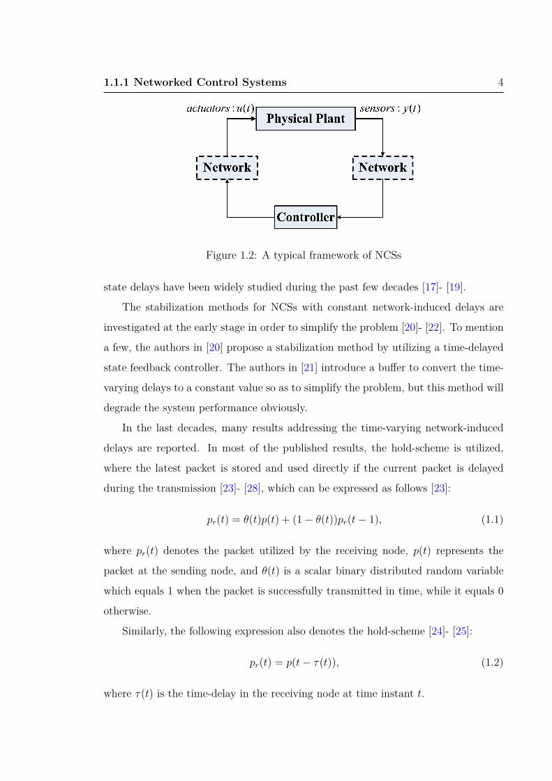
1.1.1 Networked Control Systems 4
Figure 1.2: A typical framework of NCSs
state delays have been widely studied during the past few decades [17]- [19].
The stabilization methods for NCSs with constant network-induced delays are
investigated at the early stage in order to simplify the problem [20]- [22]. To mention
a few, the authors in [20] propose a stabilization method by utilizing a time-delayed
state feedback controller. The authors in [21] introduce a buffer to convert the time-
varying delays to a constant value so as to simplify the problem, but this method will
degrade the system performance obviously.
In the last decades, many results addressing the time-varying network-induced
delays are reported. In most of the published results, the hold-scheme is utilized,
where the latest packet is stored and used directly if the current packet is delayed
during the transmission [23]- [28], which can be expressed as follows [23]:
pr(t) = θ(t)p(t) + (1− θ(t))pr(t− 1), (1.1)
where pr(t) denotes the packet utilized by the receiving node, p(t) represents the
packet at the sending node, and θ(t) is a scalar binary distributed random variable
which equals 1 when the packet is successfully transmitted in time, while it equals 0
otherwise.
Similarly, the following expression also denotes the hold-scheme [24]- [25]:
pr(t) = p(t− τ(t)), (1.2)
where τ(t) is the time-delay in the receiving node at time instant t.

1.1.1 Networked Control Systems 5
Remark 1.1. It is noted that the packet p(t) in (1.1)-(1.2) can be system states
x(t), outputs y(t) and inputs u(t), representing different filtering/control cases and
communication channels.
Different from the hold strategy, the authors in [26] propose a predictive method
for the NCSs with random network delays in both forward and feedback channels.
In addition, the authors in [29] propose a compensation method for systems with
random delays in S/C channel based on the compensation strategy.
Packet Dropouts
Packet dropout is another critical problem for NCSs, which occurs when there
are packet collisions, buffer overflows and other network congestions [5]. Obviously,
packet dropout phenomena will degrade the performance of control systems or even
make them unstable in some cases. To deal with this problem, many results have
been presented [4]- [7], [30]- [32].
Many approaches to modeling NCSs with packet dropouts have been reported.
To mention a few, the authors in [30] consider the Markovian packet loss process, and
they model the packet dropouts as a discrete-time Markov chain with given transition
probability matrix. The authors in [31] model the systems with packet dropouts as
switching systems depending on whether the packets are successfully transmitted
or not. The authors in [7], [33]- [34] model the systems with packet dropouts as
asynchronous dynamic systems.
All these methods for modeling the packet dropout phenomena can be classified
into two categories. One can be called zero strategy [7], [32], and they have the
following mathematical expression:
pr(t) = α(t)p(t), (1.3)
where pr(t) denotes the packet utilized by the receiving node, p(t) represents the
packet at the sending node, and α(t) is a scalar binary distributed random variable
which equals 1 when the packet is successfully transmitted, while it equals 0 otherwise.

1.1.1 Networked Control Systems 6
The other category can be called hold strategy [30], [31], in which the data at the
last time instant are held when the current packet is lost during the transmission.
They can be expressed as follows:
pr(t) = α(t)p(t) + (1− α(t))pr(t− 1). (1.4)
When the multiple packet dropouts are considered, the following model is also
applied [33]- [35].
pr(t) = α(t)p(t) + (1− α(t))α(t− 1)p(t− 1) + · · ·
+(1− α(t))(1− α(t− 1)) · · · (1− α(t− T + 2))α(t− T + 1)p(t− T + 1)
+(1− α(t))(1− α(t− 1)) · · · (1− α(t− T + 1))α(t− T )p(t− T ), (1.5)
where T is the maximum delay steps.
Quantization
The data need to be quantized before being transmitted through the
communication links because of the limited network bandwidth [36]- [38]. The
signals are converted into several discrete values selected from a finite set during
the quantization procedure. It is obvious that quantization errors arise due to the
finite number of bits, which will degrade the system performance.
There are numerous quantization approaches, however, just a few of them are
widely utilized for filtering and control tasks. Logarithmic quantizer and uniform
quantizer are two widely used quantizers. The logarithmic quantizer is expressed as
follows [36]- [37]:
qL(v) =
sgn(v)Vi if Vi
1+∆< |v| ≤ Vi
1−∆
0 if v = 0,(1.6)
where Vi = ρiV0, i = 0,±1,±2, · · · , 0 < ρ < 1, V0 is a positive scaling constant,
∆ = 1−ρ1+ρ
, and sgn(.) is a sign function satisfying
sgn(v) =
1 if v > 0
−1 if v < 0
0 if v = 0.
(1.7)

1.1.1 Networked Control Systems 7
The corresponding quantization error satisfies:
qL(v)− v = δv, (1.8)
where δ ∈ [−∆,∆].
Logarithmic quantizaters provide a sector bound method to deal with the
quantization errors, and have been widely used in various control and filtering
problems [36]- [37].
The other typical quantizer is the uniform quantizer, wihch is described as follows
[39]:
qU(v) =
sgn(v)⌊2N−1v⌋+0.5
2N−1 if |v| < v;
sgn(v)(1− 0.5
2N−1 v)
if |v| = v(1.9)
where v > 0 is the given constant quantizer limitation, N is the number of given
quantization bits and ⌊x⌋ = maxz ∈ Z, z ≤ x.
The corresponding quantization error is obtained as |qU(v)− v| ≤ v2N−1 .
However, the uniform quantizer mentioned above cannot solve the saturation and
dead zone problems arising from quantization [37]. In order to solve those problems,
the authors in [37] present a dynamic quantization scheme, which is expressed as
follows:
qµ(z) = µq
(z
µ
), (1.10)
where µ > 0 is a ”zoom” variable, with which the quantizer can deal with both large
and small variables.
Media Access Constraints
Due to limited communication resources, the media access constraint problem is
another network-induced issue to be considered in NCSs [43]. It is unpractical to
transmit all the packets from different nodes sharing with one communication link at
each time instant t. Therefore, it is desirable to reduce the transmission frequency of
each sending node in order to guarantee the utilization of every node. It will be more
important when the cost of the network access is high, such as the wireless networks.

1.1.1 Networked Control Systems 8
Figure 1.3: One structure of the event-triggered NCSs
Considering this issue, event-triggered and self-triggered systems have attracted much
research attention in recent years [43]- [52].
A typical structure of the event-triggered NCSs is illustrated in Figure 1.3, where
“ETM” part stands for the event-triggered mechanism. The basic idea of event-
triggered systems is to detect a designed triggering condition. If the condition is
satisfied at time instant t, then the ETM sends the packet through the network.
Otherwise, no packets will be transmitted. A commonly used event-triggering
condition is as follows [40],
∥es(t)∥2 < δ∥s(t)∥, t ∈ [tk, tk+1), (1.11)
where es(t) = s(tk) − s(t), t ∈ [tk, tk+1) is the error vector, and s(t) can be system
states x(t) and outputs y(t), representing different triggering mechanisms.
The triggering condition means that the ETM broadcasts the packet only if the
error between the current value and the last updated value is larger than a threshold.
By this means, the packets transmitted through the network could be greatly reduced.
It is claimed in [41] that the numbers of packets needed to be transmitted are less
than those utilizing periodic sampling.
Noting from (1.11), the ETMs are required to monitor the triggering condition
all the time, which needs a dedicated hardware for this purpose. However, this is
not always practical. In this case, self-triggered control is alternative [42]. The main

1.1.1 Networked Control Systems 9
idea of self-triggered control is to compute the next sampling and broadcasting time
instant of the sending node at the current time instant t.
Most of the existing literatures consider the event-triggered and self-triggered
control without the considerations of the network-indueced issues [40], [43]- [51].
To mention a few, the authors in [51] examine a class of real-time control systems
in which each control task triggers its next release based on the value of the last
sampled state. Considering event-triggered control and self-triggered control, the
authors in [47] present a new technique for the computation of the execution instants
by exploiting the concept of isochronous manifolds. The authors in [48] propose a
method by using the current state of the plant to decide the next time instant, and this
technique is developed for two classes of nonlinear control systems, state-dependent
homogeneous systems and polynomial systems. The authors in [50] investigate the
observer-based controllers for linear systems and propose advanced event-triggering
mechanisms that will reduce communication in both S/C and C/A channels. The
main idea of ETMs is the utilization of a Luenberger observer at the sensor node,
and the use of a model-based open-loop predictor that runs both at the sensor and
controller node.
In the meantime, some literatures on event-triggered and self-triggered control
consider the analysis problems [44]- [49]. For example, the following linear time-
invariant system is considered in [46]
x(t) = Ax(t) +B1u(t) +B2w(t), (1.12)
and it is assumed that there exists an H∞ controller u(t) = −BT1 Px(t) that
asymptotically stabilizes the unforced system, where P is a symmetric positive semi-
definite matrix satisfying the H∞ algebraic Riccati equation (ARE):
0 = PA+ ATP − PB1BT1 P + I + 1
γ2PB2B
T2 P. (1.13)
Different from those results that use known control laws in advance, the authors
in [43] propose a co-design method for the event generator and controller for event-
triggered control systems. Applying the LMI techniques, a sufficient condition for

1.1.1 Networked Control Systems 10
the existence of the event-triggered controller and event generator is established. A
similar co-design method is also used in [41].
Joint Network-induced Issues
The results reviewed above focus on the stabilization and filtering problems
considering one particular issue of network-based systems to simplify the problem to
be addressed. However, most of those issues will appear simultaneously in practice,
and their simultaneous consideration is thus warranted and more practical..
The authors in [53] consider the modelling and control of NCSs with both
network-induced delays and packet dropouts. A switched linear system model is
proposed to describe the NCS, and a sufficient condition is derived for the exponential
stability of the closed-loop system. The authors in [54] present the optimal estimation
results of NCS subject to random delays and packet dropouts. The authors in [55]
investigate the problem of H∞ filtering for network-based filtering systems subject
to quantization and packet dropouts. Based on a piecewise Lyapunov functional,
the approach to the design of H∞ piecewise filter is proposed such that the filtering
error system is stochastically stable with a guaranteed H∞ performance. The authors
in [56] address the filtering problems for linear NCSs with packet dropouts, network-
induced delays and quantization. The authors in [39] present a controller design
method for a class of linear network-based systems with communication constraints
in both S/C and C/A channels, where network-induced delays, packet dropouts and
quantization are considered simultaneously. The bounded stability of the closed-loop
control system is obtained via the uniform quantization method.
Some results are also presented for the event-triggered control methods with
network issues. The authors in [45] examine event-triggered dada transmission in
distributed networked control systems with packet loss and transmission delays. A
distributed event-triggering scheme is proposed, where a subsystem broadcasts its
state information to its neighbors only when the subsystems’s local state error exceeds
a specified threshold. Considering the packet dropouts and network-induced delays,
a maximal allowable number of successive dropouts (MANSD) and a bound on delays

1.1.2 Networked Nonlinear Systems via T-S Fuzzy Models 11
are provided. The authors in [41] propose a discrete event-triggered communication
scheme for a class of networked T-S fuzzy systems with bounded network-induced
delays. The main contribution is that the proposed scheme does not need a continuous
measurement and computation, and system states are only measured and checked at
a constant sampling period. However, it is noted that the method proposed in [41]
still need to sample and compute at constant time instants. Moreover, it is not
practical for the controller to obtain the premise variables of the physical plant.
The authors in [52] combine the model-based networked control systems and event-
triggered control, and the proposed framework is utilized for the stabilization of
uncertain dynamical systems and is extended to systems subject to quantization and
time-varying network delays.
1.1.2 Networked Nonlinear Systems via T-S Fuzzy Models
Fuzzy logic and fuzzy control have attracted great research attention since Zadeh
published his results on fuzzy sets [59]- [63]. However, those fuzzy controllers are
almost applied in a trial-and-error manner and lack systematic design methods at
the early stage of the research on fuzzy control.
In recent decades, great efforts on fuzzy logic have been devoted to model-based
fuzzy control systems, which provide a powerful platform for systematic stability
analysis and controller design. Among those different fuzzy models, dynamic T-S
fuzzy models have been widely studied for their great approximation capacity to
nonlinear systems. The dynamic T-S fuzzy model describes a nonlinear system by a
group of fuzzy IF-THEN rules in the form of local linear or affine models which are
smoothly connected by fuzzy membership functions, which is shown as follows:
Plant Rule Rl: IF θ1(t) is F l1 and θ2(t) is F l
2 and · · · and θv(t) is F lv, THEN x(t+ 1) = Alx(t) + Blu(t)
y(t) = Clx(t), l ∈ I := 1, 2, ..., r,(1.14)
where Rl denotes the lth fuzzy inference rule, r the number of inference rules, F lφ(φ =
1, 2, ..., v) the fuzzy sets, x(t) ∈ ℜnx the state vector, y(t) ∈ ℜnz the output vector,
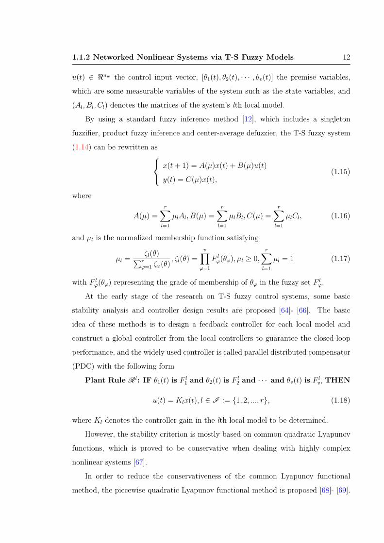
1.1.2 Networked Nonlinear Systems via T-S Fuzzy Models 12
u(t) ∈ ℜnw the control input vector, [θ1(t), θ2(t), · · · , θv(t)] the premise variables,
which are some measurable variables of the system such as the state variables, and
(Al, Bl, Cl) denotes the matrices of the system’s lth local model.
By using a standard fuzzy inference method [12], which includes a singleton
fuzzifier, product fuzzy inference and center-average defuzzier, the T-S fuzzy system
(1.14) can be rewritten as x(t+ 1) = A(µ)x(t) +B(µ)u(t)
y(t) = C(µ)x(t),(1.15)
where
A(µ) =r∑
l=1
µlAl, B(µ) =r∑
l=1
µlBl, C(µ) =r∑
l=1
µlCl, (1.16)
and µl is the normalized membership function satisfying
µl =ζl(θ)∑r
φ=1 ζφ(θ), ζl(θ) =
v∏φ=1
F lφ(θφ), µl ≥ 0,
r∑l=1
µl = 1 (1.17)
with F lφ(θφ) representing the grade of membership of θφ in the fuzzy set F l
φ.
At the early stage of the research on T-S fuzzy control systems, some basic
stability analysis and controller design results are proposed [64]- [66]. The basic
idea of these methods is to design a feedback controller for each local model and
construct a global controller from the local controllers to guarantee the closed-loop
performance, and the widely used controller is called parallel distributed compensator
(PDC) with the following form
Plant Rule Rl: IF θ1(t) is F l1 and θ2(t) is F l
2 and · · · and θv(t) is F lv, THEN
u(t) = Klx(t), l ∈ I := 1, 2, ..., r, (1.18)
where Kl denotes the controller gain in the lth local model to be determined.
However, the stability criterion is mostly based on common quadratic Lyapunov
functions, which is proved to be conservative when dealing with highly complex
nonlinear systems [67].
In order to reduce the conservativeness of the common Lyapunov functional
method, the piecewise quadratic Lyapunov functional method is proposed [68]- [69].

1.1.2 Networked Nonlinear Systems via T-S Fuzzy Models 13
After partitioning the fuzzy system (1.15) into several polyhedral regions Sii∈I
according to the membership functions, the following subsystems in each region is
obtained x(t+ 1) = Aix(t) + Biu(t)
y(t) = Cix(t),(1.19)
where
Ai =∑
m∈ℵ(i)
µmAm,Bi =∑
m∈ℵ(i)
µmBm, Ci =∑
m∈ℵ(i)
µmCm, (1.20)
with 0 ≤ µm(θ(t)) ≤ 1,∑
m∈ℵ(i) µm(θ(t)) = 1, i ∈ I ,.
Different from the controller (1.18), the following piecewise controller is utilized
u(t) = Kix(t), (1.21)
where Ki denotes the controller gain in Region Si to be determined.
The other less conservative method is based on fuzzy quadratic Lyapunov
functions [70]. It is also able to deal with a wider class of fuzzy systems than
those based on common quadratic Lyapunov functions because common Lyapunov
functions are the special case of fuzzy ones.
For networked nonlinear systems via T-S fuzzy dynamic models, most of the
existing literatures assume that the premise variables of the physical plant are always
available at the controller node, and then utilize a parallel distributed compensator
(PDC) as the controller to stabilize the physical plant [32], [71]- [77]. Similarly,
for networked nonlinear filtering systems via T-S fuzzy dynamic models, the authors
in [55] also assume that the partition information of the premise variables are available
at the filter node. However, the authors in [75]- [76] claim that these assumptions are
unpractical and propose a new asynchronous scheme, which considers the situation
when premise variables of the physical plant and fuzzy observer are in different
partition regions. Applying the compensation strategy, the authors in [29] also utilize
the asynchronous premise variables between sending and receiving nodes.

1.2 Thesis Outline and Contributions Overview 14
1.2 Thesis Outline and Contributions Overview
It the previous section, we have introduced the fundamentals of networked
control systems with limited communication capacity, and a large number of existing
results focused on the NCSs with various network-induced issues have been reviewed.
However, it is noted that there are still many important problems to be addressed.
(i) To simply the communication constraint problems of networked control systems in
most existing works, the network communication is assumed to exist in one channel,
either form the sensor to the controller or from the controller to the actuator. (ii)
Most of the existing results on the stabilization or estimation problems of network-
based systems only consider one or two network issues to simplify the concerned
problems, and few of them address those typical network problems simultaneously.
(iii) To deal with the quantization issue, the logarithmic quantizers are widely used
and the corresponding sector bound method is utilized to treat the quantization
errors. It should be noted that this kind of quantization method needs infinite
network bandwidth, which is on the contrary to the objective of the quantization
procedure. Otherwise, only bounded stability of the closed-loop system can be
achieved. (iv) Most of the existing methods treat the network-induced delays and
packet dropouts with either zero or hold strategies, but the performance of the closed-
loop NCSs is unsatisfactory when either of them is adopted. Motivated by these
issues on the research of network-based systems, this thesis will focus on analysis
and synthesis problems of NCSs considering various communication constraints. The
main contributions of this thesis are outlined as follows.
Chapter 2 considers the problem of output feedback control for network-
based discrete-time systems under unreliable communications subject to packet
dropouts, network-induced delays, and quantization. The network issues in both
sensor-to-controller (S/C) and controller-to-actuator (C/A) channels are addressed
simultaneously in a unified framework. Different from the existing results, a new
asynchronous quantization scheme is proposed, which does not need synchronous
quantization parameters between sending and receiving nodes. A dynamic output

1.2 Thesis Outline and Contributions Overview 15
feedback controller with the new quantization scheme is then designed and it is shown
that the resulting networked closed-loop control system is asymptotically stable.
Chapter 3 considers the problem of H∞ state feedback control for networked
nonlinear systems under unreliable communication links with packet dropouts. The
nonlinear plant in this chapter is described by a Takagi-Sugeno (T-S) fuzzy model.
The packet dropouts in both S/C and C/A channels are considered, which are
modeled by Bernoulli processes. A new compensation scheme for the estimation of
missing packets is proposed, and a piecewise state feedback controller is designed
so that the resulting closed-loop control system is stochastically stable with a
guaranteed H∞ performance. The system performance is improved by the proposed
compensation scheme in comparison to the existing methods. Then the results are
extended to the case when both network-induced delays and packet dropouts exist
in communication links.
Chapter 4 addresses the problem of H∞ filter design for networked nonlinear
systems under unreliable communication links with packet dropouts, network-induced
delays and quantization. The nonlinear plant in this chapter is described by a T-S
fuzzy dynamic model, and these three network constraints are treated in a unified
framework simultaneously. The network-induced delays and packet dropouts are
modeled by the time-delays in the buffers at the receiving node. A piecewise filter
is designed without knowing the region information of the premise variables of the
physical plant. Based on a piecewise quadratic Lyapunov functional, the overall
filtering error system is proved to be asymptotically stable with a guaranteed H∞
performance.
Chapter 5 considers the fuzzy modeling and H∞ state feedback control for
network-based quadrotor under unreliable communications. Both the network-
induced delays and packet dropouts are addressed. The networked nonlinear
quadrotor in this chapter is firstly approximated by a T-S fuzzy dynamic model.
The network-induced delays and packet dropouts in both S/C and C/A channels
are modeled in a unified framework. Then a fuzzy controller is designed so that the
resulting closed-loop quadrotor system is asymptotically stable with a guaranteed

1.2 Thesis Outline and Contributions Overview 16
H∞ performance.

Chapter 2
A Novel Asynchronous
Quantization Scheme for Output
Feedback Control of Networked
Control Systems
2.1 Introduction
As mentioned in Chapter 1, most of the researchers focus on just one or two
network-induced issues of NCSs in order to simplify the problem to be addressed. The
authors in [39] consider three typical network issues simultaneously, which are packet
dropouts, network-induced delays and quantization, but only bounded stability of
the closed-loop control system is obtained via the uniform quantization method.
It is noted that quantization is one of the critical issues of NCSs because data
cannot be accurately transmitted due to the limited bandwidth of communication
links [99]. Uniform quantizers and logarithmic quantizers are two widely used
quantizers in control area. With the uniform quantizer, the solutions of the control
system are shown to converge to an ellipsoid rather than zero in [39], in other words,
the asymptotic stability of the system cannot be achieved. On the other hand,
the widely used logarithmic quantizer requires infinite network bandwidth when

2.1 Introduction 18
the system approaches its equilibrium [85] [94] [101]- [102], and this is contrary
to the original purpose of quantization. In addition, a finite-level logarithmic
quantizer is proposed in [104], but it is assumed that the ”zoom” variables should be
synchronized between the sending and receiving nodes. More recently, some results on
quantization with mismatched encoder/decoder are reported [105]- [106]. However,
all of the results on quantization mentioned above are under the assumption of perfect
transmissions, which is hard to be the case in network circumstances. It is thus of
both theoretical and practical significance to consider new quantization schemes in
order to achieve the asymptotical stability of the system under the unreliable network
environment in practice, which motivates our research.
In this chapter, we propose a new logarithmic quantization scheme for NCSs.
It is shown that the closed-loop control system is asymptotically stable with the
proposed quantizer and observer-based output feedback controller, and none of the
synchronized scaling parameters between the sending and receiving nodes are needed.
Moreover, those three typical network-induced issues in both S/C and C/A channels
are modeled in a unified framework simultaneously. The contributions of this chapter
can be summarized as follows: 1) a new asynchronous quantization scheme for
networked control systems is proposed; 2) three typical network issues in both S/C
and C/A channels are considered simultaneously; and 3) different from the existing
results, the asymptotical stability of the networked closed-loop control system can be
guaranteed by utilizing the proposed quantization scheme.
The remainder of the chapter is organized as follows. Section II is devoted to the
description of the new quantization scheme and the problem formulation. Section III
presents the analysis and synthesis results based on a quadratic Lyapunov-Krasovskii
functional. In Section IV, a simulation example is given to illustrate the effectiveness
of the proposed scheme. Finally, a conclusion is drawn in section V.

2.2 Model Description 19
Figure 2.1: Structure of the closed-loop networked control system
2.2 Model Description
In this chapter, we focus on discrete-time linear systems with quantization,
packet dropouts, and network-induced delays in communication links as illustrated
in Fig.2.1. Note that all the network issues exist in both S/C and C/A channels.
Therefore, the packet at the sending and receiving nodes in both channels are not
the same. Now, we model the physical plant, quantizers and observer-based output
feedback controller mathematically.
2.2.1 Physical Plant
The linear physical plant considered in this chapter is given by: x(t+ 1) = Ax(t) +Bu(t)
y(t) = Cx(t),(2.1)
where x(t) ∈ ℜnx represents the state vector, u(t) ∈ ℜnu the input vector, y(t) ∈ ℜnz
the output vector, and (A,B,C) denote the matrices of the system.

2.2.2 Quantization 20
2.2.2 Quantization
Due to the limited bandwidth of communication links, information needs to be
quantized at the sending node before it is transmitted through the network. The
widely used logarithmic quantizer is expressed as follows [94]:
Q(v) =
sgn(v)ρiV0 if ρiV0
1+∆< |v| ≤ ρiV0
1−∆
0 if v = 0,(2.2)
where 0 < ρ < 1, V0 is a positive scaling constant, i = 0,±1,±2, · · · , ∆ = 1−ρ1+ρ
, and
sgn(.) is a sign function satisfying
sgn(v) =
1 if v > 0
−1 if v < 0
0 if v = 0.
(2.3)
The corresponding quantization error satisfies:
Q(v)− v = δv, (2.4)
where δ ∈ [−∆,∆], and we have Q(v) = (δ + 1)v.
It is noted that the value of i approaches infinity in (2.2) as |v| decreases to zero,
which indicates that the infinite number of quantization levels is needed by using
the logarithmic quantizer. Obviously, it is unpractical to implement the infinite-
level logarithmic quantizer (2.2) in practical situations. To address this problem, the
logarithmic quantizer (2.2) is improved in [104] as follows:
q(v) =
sgn(v)V0 if |v| > V0
1−∆
sgn(v)ρiV0 if ρiV0
1+∆< |v| ≤ ρiV0
1−∆
sgn(v)ρNV0 if |v| ≤ ρNV0
1+∆,
(2.5)
where i = 1, 2, · · · ,N − 1.
Different from the traditional logarithmic quantizer (2.2), the maximum value of i
in (2.5) is finite, say, N −1, which makes the improved quantizer (2.5) practical to be
implemented. In order to analyze the quantization errors of the improved quantizer

2.2.2 Quantization 21
(2.5), the relationship between the two quantizers is established as follows:
q(v) =
µvQ(v) if |v| > V0
1−∆
Q(v) if ρiV0
1+∆< |v| ≤ ρiV0
1−∆
Q(v) + ϵv if |v| ≤ ρNV0
1+∆,
(2.6)
where ϵv is a parameter satisfying 0 ≤ ϵv ≤ Vmin = ρNV0, and µv = V0
Q(v)∈ (0, 1].
Similar to [39], we consider the compact set L0 such that for any v ∈ L0, a lower
bound of µv is defined as follows
µ = minµv : v ∈ L0, (2.7)
so we have µv ∈ [µ, 1].
According to (2.4) and (2.6), we obtain
q(v) =
µv(δ + 1)v if |v| > V0
1−∆
(δ + 1)v if ρiV0
1+∆< |v| ≤ ρiV0
1−∆
(δ + 1)v + ϵv if |v| ≤ ρNV0
1+∆,
(2.8)
where δ ∈ [−∆,∆].
Remark 2.1. It is noted that there still exists a non-zero term ϵv in the improved
quantizer (2.8) when the concerned networked system approaches its equilibrium,
which makes the asymptotical stability of the concerned networked system hard to
be achieved. Similar issue will happen when a uniform quantizer is utilized in the
stabilization of a given networked system, and only bounded stability can be achieved
[39].
To overcome the aforementioned difficulty, the dynamic quantization method with
zooming variables as in [103] is resorted. However, different from the synchronous
quantizers in [103], the following asynchronous quantizers in S/C and C/A channels

2.2.2 Quantization 22
are proposed respectively as follows,
gqy(g−1y) =
Syymax if |g−1y| > ymax
1−∆1
Syρi11 ymax if ρ
i11 ymax1+∆1
< |g−1y| ≤ ρi11 ymax1−∆1
SyρNy
1 ymax if |g−1y| ≤ ρNy1 ymax1+∆1
gqu(g−1uc) =
Suymax if |g−1uc| > umax
1−∆2
Suρi22 umax if ρ
i22 umax1+∆2
< |g−1uc| ≤ ρi22 umax1−∆2
SuρNu2 umax if |g−1uc| ≤ ρNu
2 umax1+∆2
,
(2.9)
where Sy = g · sgn(y), Su = g · sgn(uc), g and g denote the asynchronous scaling
parameters at the receiving and sending nodes, respectively, ymax and umax are positive
constants, 0 < ρ1, ρ2 < 1, i1 = 1, 2, · · · ,Ny − 1, i2 = 1, 2, · · · ,Nu− 1, ∆1 =1−ρ11+ρ1
, and
∆2 =1−ρ21+ρ2
.
Remark 2.2. It is noted that ymax and umax in (2.9) denote the maximum output
values of two quantizers in S/C and C/A channels, respectively, which are transmitted
through the communication links with network-induced delays and packet dropouts.
Obviously, they are not the maximum values of actual system outputs or controller
outputs.
Similar to (2.8), we have
gqy(g−1y) =
µδ+1 gg
−1y if |g−1y| > ymax1−∆1
δ+1 gg−1y if ρ
i11 ymax1+∆1
< |g−1y| ≤ ρi11 ymax1−∆1
δ+1 gg−1y + ϵy if |g−1y| ≤ ρ
Ny1 ymax1+∆1
gqu(g−1uc) =
µδ+2 gg−1uc if |g−1uc| > umax
1−∆2
δ+2 gg−1uc if ρ
i22 umax1+∆2
< |g−1uc|
≤ ρi22 umax1−∆2
δ+2 gg−1uc + ϵu if |g−1uc| ≤ ρNu
2 umax1+∆2
,
(2.10)
where δ+j = δj + 1, j = 1, 2, δ1 ∈ [−∆1,∆1], δ2 ∈ [−∆2,∆2] and µ ∈ [µ, 1].
Remark 2.3. Most results consider the dynamic quantization under the assumption
that the network communications are perfect so that the ”zoom” variables can

2.2.3 Communication Links 23
be synchronously obtained at the sending and receiving nodes [103]- [104] [107].
Nevertheless, this assumption is hard to be satisfied in practice because the network
channel is always imperfect, that is, there are network-induced delays and packet
dropouts throughout the communication, and the traditional synchronous dynamic
quantization method can not be utilized reliably. Therefore, we propose the new
asynchronous quantizers (2.9), where the scaling parameters g and g are generated
at receiving and sending nodes respectively, and their values can be different.
2.2.3 Communication Links
Note that the phenomena of packet dropouts and network-induced delays exist
both in S/C and C/A channels. Therefore, the inputs to the controller yc(t) are not
the same as the outputs of the controlled plant y(t), while the control inputs to the
plant u(t) are also different from the outputs of the controller uc(t).
It is standard to assume that there exist buffers in controller and actuator nodes,
respectively, which store the received historical packets [89]. We model the unreliable
transmission as follows:
yc(t) = gy(it)gu(jt)qy(g−1y (it)g
−1u (jt)y(it)
)u(t) = gy(it)gu(jt)qu
(g−1y (it)g
−1u (jt)uc(jt)
), (2.11)
where qy(g−1y (it)g
−1u (jt)y(it)) and qu(g−1
y (it)g−1u (jt)uc(jt)) denote the latest data stored
in the buffer of the plant and controller nodes at time instant t, respectively. gy(it),
gy(it), gu(jt) and gu(jt) are scaling parameters updated at each node satisfying gy(it+1) = gy(it)γy(it)it+1−it
gy(t) = gy(it)γy(it)t−it gu(jt+1) = gu(jt)γu(jt)
jt+1−jt
gu(t) = gu(jt)γu(jt)t−jt ,
(2.12)
where “it” and “jt” are the latest time instants when the corresponding ‘ACK’ is
received by two receiving nodes at time t, respectively.

2.2.3 Communication Links 24
The updating parameters γy(t) and γu(t) in (2.12) satisfy
γy(t) =
γy ∈ (1,∞) if
∣∣qy(g−1y (t)g−1
u (t)y(t))∣∣ = ymax
γy∈ (0, 1) if
∣∣qy(g−1y (t)g−1
u (t)y(t))∣∣ = ymin
1 Otherwise
γu(t) =
γu ∈ (1,∞) if
∣∣qu(g−1y (t)g−1
u (t)uc(t))∣∣ = umax
γu∈ (0, 1) if
∣∣qu(g−1y (t)g−1
u (t)uc(t))∣∣ = umin
1 Otherwise,
(2.13)
where ymin = ρNyymax and umin = ρNuumax.
We define
η1(t) = t− it, η2(t) = t− jt, (2.14)
where η1(t) and η2(t) are the time-delays of the packets in the controller and actuator
nodes due to the network-induced delays and packet dropouts, respectively.
The following assumption is needed on modeling the random time-delays in the
buffers caused by the unreliable transmission.
Assumption 2.1. The time-delays η1(t) and η2(t) are time varying and satisfy 0 ≤
η1(t) ≤ η1, 0 ≤ η2(t) ≤ η2, where η1 and η2 represent the upper bounds of the
time-delays in the buffers of these two different nodes, respectively.
Remark 2.4. A time stamp is added to the packet before it is transmitted through
the network links in both S/C and C/A channels, and the network delays η1(t)
and η2(t) are measurable by comparing the time stamp of the latest received packet
with the current time instant. An ”ACK” signal representing the acknowledgement
of the packet will be transmitted to the sending node once the packet arrives at the
receiving node, and then both nodes acknowledge that the latest package information
is transmitted successfully. It is natural to assume that the ”ACK” signal has a
high priority identifier so that it can be transmitted and received without delay and
loss [108].
Remark 2.5. It is noted from (2.12) that we are able to ”zoom” the corresponding
variables at the receiving and sending nodes separately, and they are updated
asynchronously.

2.2.3 Communication Links 25
Proposition 2.1. Consider the asynchronous zooming variables between the sending
and receiving nodes in (2.12), the following bounded condition holds:
g0≤ gη(t)
gη(t)≤ g0, (2.15)
where
gη(t) = gu(t− η2(t))gy(t− η1(t))
gη(t) = gu(t− η2(t))gy(t− η1(t))
g0=γ η1yγ η2u
γ η1y γη2u
, g0 = g−1
0. (2.16)
Proof. From (2.12) we have
gy(it) = gy(it−1)γy(it−1)it−it−1
= gy(it−2)γy(it−2)it−1−it−2γy(it−1)
it−it−1
= · · ·
= gy(it−s)γy(it−s)it−s+1−it−s · · · γy(ti−1)
it−it−1 ,
while
gy(it) = gy(it−s)γy(it−s)it−it−s , (2.17)
where it−s denotes the latest time instant when an “ACK” signal is received at time
it. Obviously, it − it−s ≤ η1.
Therefore, we obtain
gy(it)
gy(it)=
γy(it−s)it−s+1−it−s · · · γy(ti−1)
it−it−1
γy(it−s)it−it−s
∈
[(γy
γy
)η1
,
(γyγy
)η1]. (2.18)
Similarly, we also have
gu(jt)
gu(jt)=
γu(jt−s)jt−s+1−jt−s · · · γu(tj−1)
jt−jt−1
γu(jt−s)jt−jt−s
∈
[(γu
γu
)η2
,
(γuγu
)η2]. (2.19)

2.2.4 Observer 26
Noting it = t− η1(t) and jt = t− η2(t), we obtain(γy
γy
)η1
≤ gy(t− η1(t))
gy(t− η1(t))≤
(γyγy
)η1
(γu
γu
)η2
≤ gu(t− η2(t))
gu(t− η2(t))≤
(γuγu
)η2
, (2.20)
which implies
g0≤ gη(t)
gη(t)≤ g0, (2.21)
and thus the proof is completed.
2.2.4 Observer
Based on the system (2.1), we consider the following observer.
x(t+ 1) = Ax(t) +Ryc(t), (2.22)
where x(t) is the estimated state; A and R are observer gains to be determined.
2.2.5 Controller
Based on the observer (2.22), we consider the following controller
uc(t) = Kx(t), (2.23)
where K is the controller gain to be determined.
2.2.6 Closed-loop System
Then from (2.1), (2.11), (2.20)-(2.23), we have the following closed-loop system: x(t+ 1) = Ax(t) + gη(t)Bqu(g−1η (t)Kx(t− η2(t))
)x(t+ 1) = Ax(t) + gη(t)Rqy
(g−1η (t)Cx(t− η1(t))
).
(2.24)
It is noted that (2.24) can be rewritten as follows: x(t+ 1) = Ax(t) + gη(t)
gη(t)Bgη(t)qu
(g−1η (t)Kx(t− η2(t))
)x(t+ 1) = Ax(t) + gη(t)
gη(t)Rgη(t)qy
(g−1η (t)Cx(t− η1(t))
).
(2.25)

2.3 Main Results 27
The problem to be addressed in this chapter is described as follows:
Dynamic Output Feedback Controller Design Problem. Consider the
linear system (2.1) and suppose that the network parameters η1 and η2 are given.
Design the observer-based output feedback controller in the form of (2.22) and (2.23)
such that the augmented system (2.25) is asymptotically stable.
2.3 Main Results
In this section, the solutions to the problem described in the last section will
be given in the framework of the linear matrix inequality (LMI) approach based on
Lyapunov-Krasovskii functional.
Before proceeding further, the following lemmas are introduced.
Lemma 2.2. [109] For matrices H and E, and scalar ε > 0, the following inequality
holds:
HFE + ETF THT ≤ εHHT + ε−1ETE, (2.26)
where F satisfies F TF ≤ I.
Lemma 2.3. [110] Given appropriately dimensioned matrices Ω1,Ω2, and Ω3 with
Ω1 = ΩT1 , then
Ω1 + Ω3Υ(k)Ω2 + ΩT2Υ
T (k)ΩT3 < 0 (2.27)
holds for all Υ(k) satisfying ΥT (k)Υ(k) ≤ I if and only if for some ε > 0
Ω1 + ε−1Ω3ΩT3 + εΩT
2Ω2 < 0. (2.28)
Consider the closed-loop control system (2.25), where an improved quantization
scheme (2.9) with (2.12) is utilized.
We define z(t) = g−1y (t)g−1
u (t)x(t)
z(t) = g−1y (t)g−1
u (t)x(t),(2.29)

2.3 Main Results 28
and (2.25) can be rewritten as follows
z(t+ 1) = γ−η2(t)−1u
γ−η1(t)−1y
·[γη2(t)u
γη1(t)y
Az(t) + gη(t)
gη(t)gη(t)Bqu
(g−1η (t)Kx(t− η2(t))
)]z(t+ 1) = γ
−η2(t)−1u γ
−η1(t)−1y ·[
γη2(t)u γ
η1(t)y Az(t) + gη(t)
gη(t)gη(t)Rqy
(g−1η (t)Cx(t− η1(t))
)].
We consider the following Lyapunov-Krasovskii functional candidate
V (t) = V1(t) + V2(t) + V3(t), (2.30)
where
V1(t) = zT (t)P1z(t) + zT (t)P2z(t)
V2(t) =−1∑
q=−η1
t−1∑p=t+q
ea(p−t+1)zT (p)Q1z(p)
+−1∑
q=−η2
t−1∑p=t+q
ea(p−t+1)zT (p)Q2z(p)
+−1∑
q=−η2
t−1∑p=t+q
ea(p−t+1)zT (p)Q3z(p)
V3(t) =−1∑
q=−η1
t−1∑p=t+q
ea(p−t+1)dT (p)Z1d(p)
+−1∑
q=−η2
t−1∑p=t+q
ea(p−t+1)dT (p)Z2d(p)
+−1∑
q=−η2
t−1∑p=t+q
ea(p−t+1)dT (p)Z3d(p), (2.31)
d(t) = z(t+1)− z(t), d(t) = z(t+1)− z(t), z(t) = z(t)− z(t), and Pj = P Tj > 0, j =
1, 2, Qi = QTi > 0, Zi = ZT
i > 0, i = 1, 2, 3. Then we have the following result.
Lemma 2.4. Consider the system (2.1) and the improved quantizer (2.9). Then,
for any initial state x(0) and t ≥ 0, the following inequality (2.32) holds if there
exist matrices M,N, S, Pj = P Tj > 0, j = 1, 2, Qi = QT
i > 0, Zi = ZTi > 0, i =

2.3 Main Results 29
1, 2, 3, ε1, ε2, εB, εC > 0 satisfying Θ < 0,
V (t+ 1) <
e−aV (t) if the system is in S1
e−aV (t) + ϵ21 if the system is in S2
e−aV (t) + ϵ22 if the system is in S3
e−aV (t) + ϵ23 if the system is in S4,
(2.32)
where a is a positive constant, and
S1 :x(t), x(t)|ymin <
∣∣qy(g−1η (t)y(tη1))
∣∣ ≤ ymax
and umin <∣∣qu(g−1
η (t)uc(tη2))∣∣ ≤ umax
S2 :
x(t), x(t)|ymin <
∣∣qy(g−1η (t)y(tη1))
∣∣ ≤ ymax and∣∣qu(g−1
η (t)uc(tη2))∣∣ = umin
S3 :
x(t), x(t)|umin <
∣∣qu(g−1η (t)uc(tη2))
∣∣ ≤ umax and∣∣qy(g−1
η (t)y(tη1))∣∣ = ymin
S4 :
x(t), x(t)|
∣∣qy(g−1η (t)y(tη1))
∣∣ = ymin and∣∣qu(g−1
η (t)uc(tη2))∣∣ = umin
Θ =
Π1 Π2 0 R
∗ Ψ+ Ξ + ΞT KT 0
∗ ∗ −ε2 0
∗ ∗ ∗ ε1
< 0, (2.33)
with
Π1 = diag−P−1 + ε2(∆2),−Z−1 + ε2(∆2),−e−aη1Z1,−e−aη2Z2,−e−aη2Z3
Π2 =
[ΓT1 ΓT
2
√η1M
√η2N
√η2S
]TP = diag
P1, P2
, Pj = (1 + τ)Pj, j = 1, 2
Z = diagZ12, Z3
, Z12 = (1 + τ)(η1Z1 + η2Z2), Z3 = (1 + τ)η2Z3
Ψ = diag−e−aP1 + η1Q1 + η2Q2,−e−aP2 + η2Q3,
−e−aη1Q1 + ε1(∆1),−e−aη2Q2,−e−aη2Q3

2.3 Main Results 30
Ξ =[
e−aη1M + e−aη2N e−aη2S −e−aη1M −e−aη2N −e−aη2S]
ε2(∆2) = diag2ε2Bi∆2∆
T2B
Ti + 2εBEbi∆2∆
T2E
Tbi,
2ε2Bi∆2∆T2B
Ti + 2εBEbi∆2∆
T2E
Tbi
ε1(∆1) = 2ε1C
Ti ∆
T1∆1Ci + 2εCE
Tci∆
T1∆1Eci Eb1 Eb2 Eb3
Ec1 Ec2 Ec3
=
0 δB δB
0 δC δC
ε1 =
−ε1 0
∗ −εC
, ε2 = −ε2 0
∗ −εB
Γ1 =
Ai 0 0 BiK −BiK
Ai − γjA γjA −RCj BiK −BiK
Γ2 =
Ai − I 0 0 BiK −BiK
Ai − γjA γjA− I −RCj BiK −BiK
γ1 = 1, γ2 = γ−1
uγ−1
y, γ3 = γ−1
u γ−1y
K =
0 0 0 K K
0 0 0 K K
, R =
0 RT 0 RT 0 0 0
0 RT 0 RT 0 0 0
T
A1 A2 A3
B1 B2 B3
=
A γ−1uγ−1yA γ−1
u γ−1y A
B γ0B γ0B
γ0=γ−η1−1y
γ−η2−1u
g0 + γ−1yγ−1ug0
2
γ0 =µγ−η1−1
y γ−η2−1u g
0+ γ−1
y γ−1u g0
2
δ =γ−η1−1y
γ−η2−1u
g0 − γ−1yγ−1ug0
2
δ =−µγ−η1−1
y γ−η2−1u g
0+ γ−1
y γ−1u g0
2
ϵ21 = (1 + τ−1)(γ0+ δ)2BT (P1 + P2 + η1Z1 + η2Z2 + η2Z3)Bu
2min
ϵ22 = (1 + τ−1)RT (P2 + η2Z3)Ry2min
ϵ23 = (1 + τ−1)(γ0+ δ)2BT (P1 + 2P2 + η1Z1 + η2Z2 + 2η2Z3)Bu
2min
+ (1 + τ−1)RTP2Ry2min. (2.34)
Proof. The proof procedures in different cases are similar. Without loss of generality,

2.3 Main Results 31
we just consider the proof of the case when the system is in region S2, that is,
ymin <∣∣qy(g−1
η (t)y(it))∣∣ ≤ ymax and
∣∣qu(g−1η (t)uc(jt))
∣∣ = umin.
If ymin <∣∣qy(g−1
η (t)y(iy))∣∣ < ymax, qy(g−1
η (t)y(it)) is a standard logarithmic
quantizer as (2.2), and qy(g−1η (t)y(it)) = g−1
η (t)(δ1 + 1)Cx(t − η1(t)) according to
(2.9) and (2.14). Additionally, qy(g−1η (t)y(it)) = g−1
η (t)µ(δ1 + 1)Cx(t − η1(t)) if
qy(g−1η (t)y(it)) = ymax, where µ < µ < 1. Therefore, we have
qy(g−1η (t)y(it)) = g−1
η (t)µ(δ1 + 1)Cx(t− η1(t)), (2.35)
where µ < µ ≤ 1.
Based on (2.9), (2.14) and∣∣qu(g−1
η (t)uc(jt))∣∣ = umin, we have
qu(g−1η (t)uc(jt)) = g−1
η (t)(δ2 + 1)Kx(t− η2(t)) + εu(t− η2(t)), (2.36)
where |εu(t− η2(t))| ≤ umin.
Based on (2.35) and (2.36), the closed-loop system (2.30) can be rewritten asz(t+ 1) = γ2Az(t) + γ
η(t) gη(t)
gη(t)B(δ2 + 1)Kz(t− η2(t))
+ γη(t) gη(t)
gη(t)Bεu(t− η2(t))
z(t+ 1) = γ3Az(t) + µR(δ1 + 1)γη(t)gη(t)
gη(t)Cz(t− η1(t)),
(2.37)
where γη(t) = γ−η2(t)−1
uγ−η1(t)−1y
and γη(t) = γ−η2(t)−1u γ
−η1(t)−1y .
Note that (2.37) can be expressed as follows:
z(t+ 1) = γ2Az(t) + (γ0B + B)(δ2 + 1)Kz(t− η2(t))
− (γ0B + B)(δ2 + 1)Kz(t− η2(t))
+ (γ0B + B)εu(t− η2(t))
z(t+ 1) = (γ2A− γ3A)z(t) + γ3Az(t)
− µR(δ1 + 1)(γ0C + C)z(t− η1(t))
+ (γ0B + B)(δ2 + 1)Kz(t− η2(t))
− (γ0B + B)(δ2 + 1)Kz(t− η2(t))
+ (γ0B + B)εu(t− η2(t)),
(2.38)
where z(t) = z(t)− z(t).
Then the original stability analysis problem is converted to a robust control
problem with parameter uncertainties in the system matrices.

2.3 Main Results 32
Define ζ(t) =[zT (t) zT (t) zT (t− η1(t)) zT (t− η2(t)) zT (t− η2(t))
]T, and
we have
V1(t+ 1) − e−aV1(t)
= zT (t+ 1)P1z(t+ 1)− e−azT (t)P1z(t)
+zT (t+ 1)P2z(t+ 1)− e−azT (t)P2z(t)
=[A+ (γ
0B + B)εu(t− η2(t))
]TP1
[A+ (γ
0B + B)εu(t− η2(t))
]+[A+ (γ
0B + B)εu(t− η2(t))
]TP2
[A+ (γ
0B + B)εu(t− η2(t))
]−e−azT (t)P1z(t)− e−azT (t)P2z(t)
≤ (1 + τ)ATP1A+ (1 + τ−1)(γ0+ δ)2BTP1Bu
2min
+(1 + τ)ATP2A+ (1 + τ−1)(γ0+ δ)2BTP2Bu
2min
−e−azT (t)P1z(t)− e−azT (t)P2z(t)
= ζT (t)ΓT1 P Γ1ζ(t)− e−azT (t)P1z(t)− e−azT (t)P2z(t) + ϵ211, (2.39)
where
A = γ2Az(t) + (γ0B + B)(δ2 + 1)Kz(t− η2(t))
−(γ0B + B)(δ2 + 1)Kz(t− η2(t))
A = (γ2A− γ3A)z(t) + γ3Az(t)− µR(δ1 + 1)(γ0C + C)z(t− η1(t))
+(γ0B + B)(δ2 + 1)Kz(t− η2(t))− (γ
0B + B)(δ2 + 1)Kz(t− η2(t)),
P = diag (1 + τ)P1, (1 + τ)P2
ϵ21 = (1 + τ−1)(γ0+ δB)
2BT (P1 + P2)Bu2min
ϵ211 = (1 + τ−1)(γ0+ δ)2BT (P1 + P2)Bu
2min
Γ1 =
γ2A 0 0
γ2A− γ3A γ3A −R(δ1 + 1)(γ0C + C)
(γ0B + B)(δ2 + 1)K −(γ
0B + B)(δ2 + 1)K
(γ0B + B)(δ2 + 1)K −(γ
0B + B)(δ2 + 1)K
. (2.40)

2.3 Main Results 33
Additionally,
V2(t+ 1) − e−aV2(t)
≤ η1zT (t)Q1z(t)− e−aη1zT (t− η1(t))Q1z(t− η1(t))
+η2zT (t)Q2z(t)− e−aη2zT (t− η2(t))Q2z(t− η2(t))
+η2zT (t)Q3z(t)− e−aη2 zT (t− η2(t))Q3z(t− η2(t)),
V3(t+ 1) − e−aV3(t)
≤ η1dT (t)Z1d(t)− e−aη1
t−1∑α=t−η1
dT (α)Z1d(α)
+η2dT (t)Z2d(t)− e−aη2
t−1∑α=t−η2
dT (α)Z2d(α)
+η2dT (t)Z3d(t)− e−aη2
t−1∑α=t−η2
dT (α)Z3d(α)
≤ η1dT (t)Z1d(t) + e−aη1 η1ζ
T (t)MZ−11 MT ζ(t)
+2ξT (t)e−aη1M [z(t)− z(t− η1(t))]
+η2dT (t)Z2d(t) + e−aη2 η2ζ
T (t)NZ−12 NT ζ(t)
+2ξT (t)e−aη2N [z(t)− z(t− η2(t))]
+η2dT (t)Z3d(t) + e−aη2 η2ζ
T (t)SZ−13 ST ζ(t)
+2ξT (t)e−aη2S [z(t)− z(t− η2(t))]
≤ ζT (t)ΓT2 ZΓ2ζ(t) + e−aη1 η1ζ
T (t)MZ−11 MT ζ(t)
+e−aη2 η2ζT (t)NZ−1
2 NT ζ(t) + e−aη2 η2ζT (t)SZ−1
3 ST ζ(t)
+ζT (t)(Ξ + ΞT
)ζ(t) + ϵ212, (2.41)
where
Γ2 =
γ2A− I 0 0
γ2A− γ3A γ3A− I −µR(δ1 + 1)(γ0C + C)
(γ0B + B)(δ2 + 1)K −(γ
0B + B)(δ2 + 1)K
(γ0B + B)(δ2 + 1)K −(γ
0B + B)(δ2 + 1)K
Z = diag (1 + τ)(η1Z1 + η2Z2), (1 + τ)η2Z3
ϵ212 = (1 + τ−1)(γ0+ δ)2BT (η1Z1 + η2Z2 + η2Z3)Bu
2min. (2.42)

2.3 Main Results 34
It then follows that (2.33) implies V1(t+1)−e−aV1(t)−ϵ21 < 0 by applying Lemma
2.2, Lemma 2.3 and the Schur complement operation. Therefore, we have V1(t+1) <
e−aV1(t) + ϵ21 in the case when ymin < |qy(y(tη1))| ≤ ymax and |qu(uc(tη2))| = umin.
Similarly, we are able to prove the other cases, and thus the proof is completed.
The following corollary can be obtained from Lemma 2.4.
Corollary 2.5. Consider the closed-loop system (2.30). z(t) = g−1y (t)g−1
u (t)x(t)
converges to the following ellipsoid for any initial state x(0) = x0,
Z∞ =z|zT (t)P1z(t) ≤ V∞
, (2.43)
where V∞ = (1− α)−1β, α = e−a, β = maxϵ21, ϵ22, ϵ23.
Proof. From Lemma 2.4, it is noted that V (t) decreases and converges to a bounded
region because 0 < e−a < 1. We denote the region as V∞, which can be obtained by
solving V∞ = αV∞ + β, where α = e−a and β = maxϵ21, ϵ22, ϵ23. Then, we have
V∞ = (1− α)−1β. (2.44)
It is noted that zT (t)P1z(t) < V (t), thus the proof is completed.
Proposition 2.6. There exists a time instant ts so that the quantizers will not be
saturated after time ts if the quantization level 2Nu and 2Ny of the quantizers in
C/A and S/C channels satisfy the following conditions respectively
Nu >1
2logρ
(1− δ)−2y2maxαK
(P−11 + P−1
2
)KT (Bu2max +Ry2max)
Ny >1
2logρ
(1− δ)−2y2maxαCP−1
1 CT (Bu2max +Ry2max), (2.45)
where B = (1 + τ−1)(γ0+ δB)
2BT (P1 + 2P2 + η1Z1 + η2Z2 + 2η2Z3)B, R = (1 +
τ−1)RT (P2 + η2Z3)R and α = (1− α)−1.
Proof. Obviously, there exists a time instant ts so that V (t) < (1−α)−1β holds for all
t > ts, because V∞ < (1−α)−1β is satisfied according to Corollary 2.5. Additionally,
we have
zT (t)P1z(t) < V∞ < (1− α)−1β
zT (t)P2z(t) < V∞ < (1− α)−1β, (2.46)

2.3 Main Results 35
which imply that
z(t)zT (t) < (1− α)−1βP−11
z(t)zT (t) < (1− α)−1βP−12 . (2.47)
It is noted that both quantizers in S/C and C/A channels will not be saturated
if the following conditions are satisfied according to (2.9)
|Cz(t)| < ymax
1− δ, |Kz(t)| < umax
1− δ, (2.48)
and the following conditions imply (2.48)
Cz(t)zT (t)CT <y2max
(1− δ)2
Kz(t)zT (t)KT +Kz(t)zT (t)KT <u2max
(1− δ)2. (2.49)
By substituting (2.47) and (2.45) into (2.49), the quantizers will not be saturated
if (2.45) is satisfied. Therefore, there exists a time instant ts such that the quantizers
in both channels will not be saturated if the quantization level Ny and Nu satisfy
(2.45), and the proof is completed.
Now, we have the following main result.
Theorem 2.1. With the improved logarithmic quantizers (2.9) with (2.12) and
tranmission scheme (2.11), the state x(t) of the closed-loop system (2.25) converges
to zero asymptotically if (2.33) and (2.45) are satisfied.
Proof. It is noted that z(t) converges to the ellipsoid Z∞ exponentially from Corollary
2.5, which implies that both quantizers in S/C and C/A channels will no longer be
saturated after time instant ts according to Proposition 2.6. It means gu(t)gy(t) will
not increase for all t > ts from (2.12) with (2.13), that is, gu(t)gy(t) will decrease or
remain unchanged.
Considering t > ts, it is noted that whenever gu(t)gy(t) remains unchanged, V (t)
will decrease exponentially until |Cz(t)| is less than ymin and/or |Kz(t)| is less than
umin according to Lemma 2.4, forcing gu(t)gy(t) to decrease finally. Therefore, the
system will finally be located at region S2, S3 or S4, which implies that gu(t)gy(t)

2.3 Main Results 36
will decrease to infinitesimal by factor γu, γ
yor γ
uγy
according to the region where
the system stays, and we obtain g−1u (t)g−1
y (t) → +∞. It is noted from (2.29) that
z(t) = g−1y (t)g−1
u (t)x(t), and we conclude x(t) → 0 as t→ 0 since z(t) is bounded for
all t > ts according to Corollary 2.5. Thus the proof is completed.
Remark 2.6. It is noted that the number of levels of the quantizers (2.9) utilized in
this chapter is finite, but the infinite quantization accuracy is able to be achieved by
using the asynchronous scaling parameters gu(t)gy(t) and gu(t)gy(t), which result in
the asymptotical stability of the concerned networked system.
Now we present the output feedback controller design method based on the
improved logarithmic quantization scheme.
It is pointed that (2.33) is not strict LMI because of the existence of P−1j , j = 1, 2,
Z−112 and Z−1
3 . By utilizing a cone complementarity linearization (CCL) algorithm [80],
we can solve this nonconvex feasibility problem by converting it into an optimization
problem with LMI constraints.
Introducing new matrices Pj, j = 1, 2, Z12 and Z3 with the following definition,
Pj = P−1j , j = 1, 2, Z12 = Z−1
12 , Z3 = Z−13 , (2.50)
we obtain the strict LMI Θ < 0 as (2.33), where P−1j , j = 1, 2, Z−1
12 and Z−13 are
replaced by Pj, j = 1, 2, Z12 and Z3, respectively. Then the problem of observer-
based output feedback controller design can be converted to the following nonlinear
minimization problem with LMI constraints
minimize Trace(∑
j
PjPj + Z12Z12 + Z3Z3
), (2.51)
subject to Pj I
∗ Pj
> 0,
Z12 I
∗ Z12
> 0,
Z3 I
∗ Z3
> 0,
Θ < 0, j ∈ 1, 2. (2.52)
Then, the above nonlinear minimization problem can be sloved by the algorithm
described as follows:

2.4 Simulation 37
Algorithm 2.1.
Step 1. Find a set of feasible matrices P 0j , j = 1, 2, Z0
12, Z03 , P 0
j , Z012, Z0
3 , A0, R0 and
K0 that satisfies the conditions in (2.52). Set σ = 0.
Step 2. Solve the following optimization problem for the variables(Pj, Z12, Z3, Pj, Z, Z3, A, R,K
):
minimize Trace(∑
j
(P σj Pj + PjP
σj ) + Zσ
12Z12 + Z12Zσ12 + Zσ
3 Z3 + Z3Zσ3
)subject to (2.52).
Set P (σ+1)j = Pj, Z(σ+1)
12 = Z12, Z(σ+1)3 = Z3, P (σ+1)
j = Pj, Z(σ+1)12 = Z12, Z(σ+1)
3 = Z3,
A(σ+1) = A, K(σ+1) = K, and R(σ+1) = R.
Step 3. With the gains A, R and K obtained in Step 2, check whether (2.33) is
feasible with respect to the matrices M,N, S, Pj = P Tj > 0, j = 1, 2, Qi = QT
i >
0, Zi = ZTi > 0, i = 1, 2, 3, ε1, ε2, εB, εC > 0. If it is feasible, the obtained gains A,
R, K are the solutions and exit. Otherwise, set σ = σ + 1, and go to Step 2. If σ
reaches the specified number of iterations, print “no solutions” and exit.
2.4 Simulation
In this section, we consider an inverted pendulum on a cart under the network
environment, where the controller and the pendulum system are connected by network
communication links. The physical model can be found in [111] and the dynamics of
the inverted pendulum system is expressed as follows:
(M +m)x+mlθcosθ −mlθ2sinθ = u
mlxcosθ + 4
3ml2θ −mglsinθ = 0, (2.53)
where M and m are the masses of the cart and the pendulum, respectively, l denotes
the half length of the pendulum, θ is the angle of the pendulum from the vertical,
u denotes the force applied to the cart, and g is the gravity acceleration. Selecting
x = [ x1 x2 ]T = [ θ θ ]T as the state variables and linearizing the physical model

2.4 Simulation 38
at the equilibrium point x = [ 0 0 ]T , we obtain the following model: x(t) = Acx(t) +Bcu(t)
y(t) = Cx(t)
where
Ac =
0 1
3(M+m)gl(4M+m)
0
, Bc =
0
− 3l(4M+m)
, C =[0.01 0.01
]In this study, the model parameters are given as M = 8.0kg, m = 2.0kg, l =
0.75m, and g = 9.8m/s2. After discretizing the above pendulum system with sampling
period Ts = 10ms, we obtain the following discrete-time system x(t+ 1) = Ax(t) +Bu(t)
y(t) = Cx(t)
where
A =
1.0006 0.0100
0.1153 1.0006
, B =
0
−0.0012
, C =[0.01 0.01
]It is noted that the open-loop system is unstable. The objective is to design
a dynamic output feedback controller under the network environment so that the
closed-loop system is asymptotically stable.
The network and quantizer parameters are chosen as follows:
η1 = η2 = 1, µ = 0.95,
γu = γy = 1.01, γu= γ
y= 0.999, ρ = 0.95, N = 128.
Applying Theorem 2.1 and Algorithm 2.1, we obtain the following output
feedback controller gains
A =
0.8142 −0.1489
−0.3460 0.6559
, R =
23.1937
29.6205
,K =
[156.6671 85.0786
].
A number of simulations with different initial conditions and randomly generated
delays have been carried out. One particular case with the initial condition x(0) =
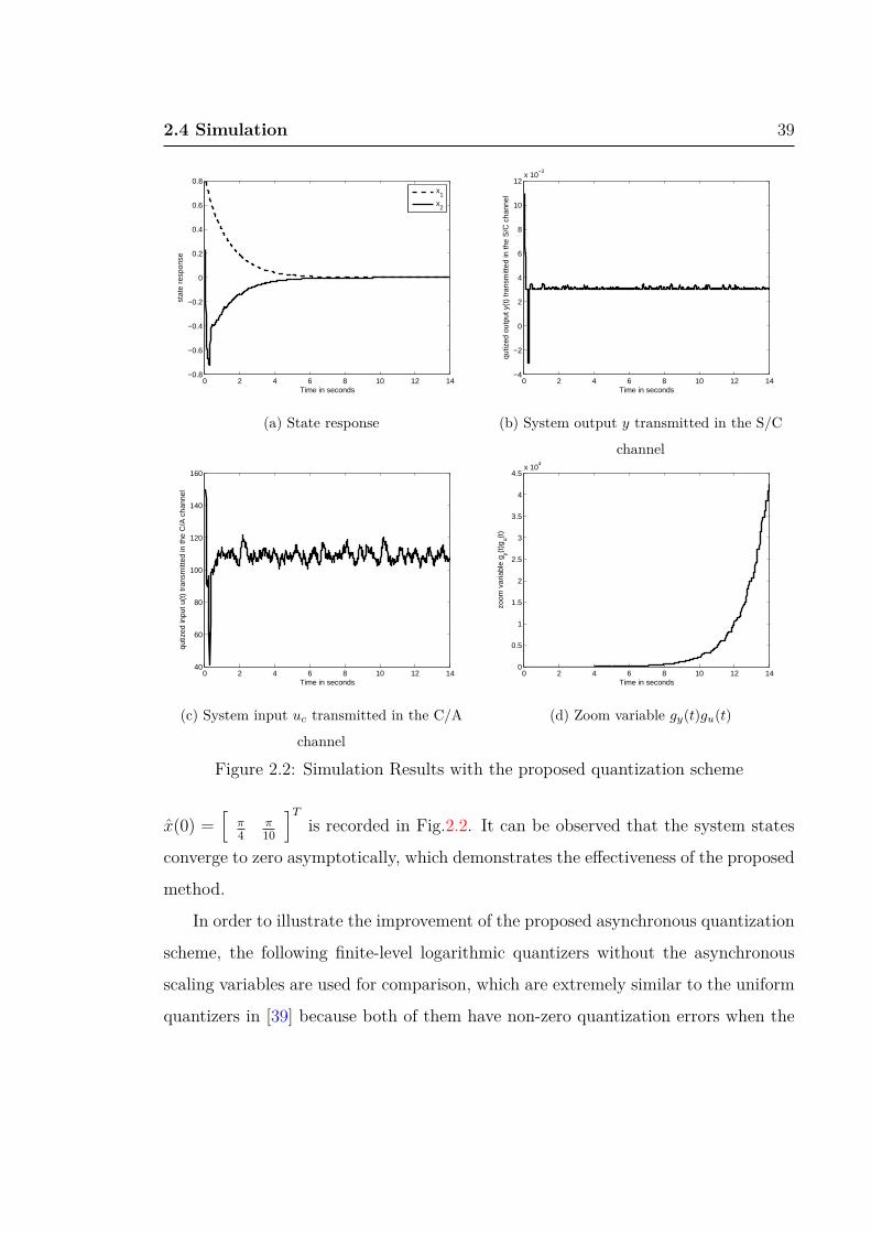
2.4 Simulation 39
0 2 4 6 8 10 12 14−0.8
−0.6
−0.4
−0.2
0
0.2
0.4
0.6
0.8
Time in seconds
stat
e re
spon
se
x
1
x2
(a) State response
0 2 4 6 8 10 12 14−4
−2
0
2
4
6
8
10
12x 10
−3
Time in seconds
qutiz
ed o
utpu
t y(t
) tr
ansm
itted
in th
e S
/C c
hann
el
(b) System output y transmitted in the S/C
channel
0 2 4 6 8 10 12 1440
60
80
100
120
140
160
Time in seconds
qutiz
ed in
put u
(t)
tran
smitt
ed in
the
C/A
cha
nnel
(c) System input uc transmitted in the C/A
channel
0 2 4 6 8 10 12 140
0.5
1
1.5
2
2.5
3
3.5
4
4.5x 10
4
Time in seconds
zoom
var
iabl
e g y(t
)gu(t
)
(d) Zoom variable gy(t)gu(t)
Figure 2.2: Simulation Results with the proposed quantization scheme
x(0) =[
π4
π10
]Tis recorded in Fig.2.2. It can be observed that the system states
converge to zero asymptotically, which demonstrates the effectiveness of the proposed
method.
In order to illustrate the improvement of the proposed asynchronous quantization
scheme, the following finite-level logarithmic quantizers without the asynchronous
scaling variables are used for comparison, which are extremely similar to the uniform
quantizers in [39] because both of them have non-zero quantization errors when the

2.5 Conclusion 40
0 2 4 6 8 10 12 14−0.8
−0.6
−0.4
−0.2
0
0.2
0.4
0.6
0.8
Time in seconds
stat
e re
spon
se
x
1
x2
Figure 2.3: State response with traditional finite-level logarithmic quantizers
concerned networked system approaches the equilibrium,
qy(y) =
sgn(y)ymax if |y| > ymax
1−∆1
sgn(y)ρi11 ymax if ρi11 ymax1+∆1
< |y| ≤ ρi11 ymax1−∆1
sgn(y)ρNy
1 ymax if |y| ≤ ρNy1 ymax1+∆1
qu(uc) =
sgn(uc)ymax if |uc| > umax
1−∆2
sgn(uc)ρi22 umax if ρi22 umax1+∆2
< |uc| ≤ ρi22 umax1−∆2
sgn(uc)ρNu2 umax if |uc| ≤ ρNu
2 umax1+∆2
.
With the same network parameters, the system states are illustrated in Fig.2.3.
It is observed that the system states only converge to the bounded region instead of
zero. It is noted that better control results are achieved by applying the proposed
asynchronous quantization scheme in comparison to the existing quantization
methods.
2.5 Conclusion
The output feedback control problem of NCSs is studied in this chapter.
A new asynchronous quantization scheme is proposed, and an observer-based
output feedback controller is designed. It is shown that the closed-loop system
is asymptotically stable even with network-induced delays, packet dropouts and
quantization in both S/C and C/A channels. Moreover, the proposed quantization

2.5 Conclusion 41
scheme does not require synchronous quantization parameters between the sending
and receiving nodes, which is more practical than the existing results. The
effectiveness of the proposed method is illustrated by the simulation of the control of
an inverted pendulum finally.
Chapter 3
A Novel Dropout Compensation
Scheme for Control of Networked
T-S Fuzzy Dynamic Systems
3.1 Introduction
In this chapter, we are interested in designing a state feedback controller for a
class of nonlinear NCSs subject to packet dropouts and network-induced delays.
It is noted that packet dropout is one of the critical problems of controller design
for NCSs, which occurs if there exist packet collisions, buffer overflows or other
network congestions [5]. The methods for modeling packet dropout phenomenon
can be classified into two categories as mentioned in Chapter 1. One is called zero
strategy [7], [32], [114], in which the missing packet is set to be zero without any
compensation. This strategy has a relatively simple mathematical expression for
analysis and synthesis of control systems, but the overall system will be open-loop
for a period of time if packets are lost continuously. Obviously, it will degrade the
system performance or even make it unstable if the packet loss rate is high. The other
is called hold strategy [30]- [31], in which the data at last sampling time are held when
the current packet is lost during the transmission. Different from the zero strategy,
it does not result in the open-loop scenario. However, the controller performance

3.1 Introduction 43
in this case might not be satisfactory if multiple packet dropouts phenomena occur,
because the system control inputs are not updated frequently enough. Therefore,
to achieve better system performance, a better strategy is needed to deal with the
packet dropout phenomenon. Moreover, most of the results on NCSs with packet
dropouts reported in literature consider only linear plants [4]- [6], [30], [126]. Though
there are some works on fuzzy-model-based nonlinear NCSs, they are all based on
zero/hold strategy [7], [76]. It is thus significant for us to consider a new strategy in
order to achieve better performance of T-S fuzzy systems under the unsatisfactory
network environment in practice, which motives our research.
In this chapter, we propose a new compensation method for fuzzy-model-based
nonlinear NCSs to deal with packet dropouts in both S/C and C/A channels.
The nonlinear physical plant is described by a T-S fuzzy model. By utilizing a
piecewise Lyapunov function method, the H∞ controller is obtained. The result is
then extended to the case when both network-induced delay and packet dropout
phenomena exist. Finally, two examples are given to show that our strategy is
effective and able to achieve better performance in comparison to the zeor/hold
strategies. The contributions of this chapter can be summarized as follows: 1) a new
approach to solving the H∞ control design problem of the T-S fuzzy control system
with packet dropouts in both S/C and C/A channels is proposed; 2) the optimal
H∞ performance is achieved by utilizing the proposed compensation approach; 3) the
proposed approaches can deal with the case when both packet dropouts and network-
induced delay phenomena exist.
The remainder of the chapter is organized as follows. Section II is devoted to
problem formulation and the description of the novel compensation strategy. Section
III presents the H∞ analysis and synthesis results based on a piecewise quadratic
Lyapunov function. Section IV presents an extension to the case when both network-
induced delay and packet dropout phenomena exist. In Section V, two simulation
examples are given to illustrate the effectiveness of the proposed approaches and show
better performance in comparison with the existing methods. Finally, a conclusion
is drawn in section VI.

3.2 Model Description and Problem Formulation 44
Figure 3.1: Structure of the networked T-S fuzzy system
3.2 Model Description and Problem Formulation
In this chapter, we focus on a class of T-S fuzzy systems with packet dropouts
in communication links as illustrated in Fig.1. Note that the packet dropout
phenomenon exists both in S/C and C/A channels. Therefore, the inputs to the
controller x(t) are not the same as the states of the controlled plant x(t), and the
control inputs to the plant u(t) are also different from the outputs of the controller
u(t). Now, we model the physical plant, dynamic compensator and controller
mathematically.
3.2.1 Physical Plant
The T-S fuzzy-model-based physical plant in this chapter is given by:
Plant Rule Rl: IF θ1(t) is F l1 and θ2(t) is F l
2 and · · · and θv(t) is F lv, THEN x(t+ 1) = Alx(t) +Blu(t) +Dlw(t)
z(t) = Llx(t) +Hlu(t), l ∈ I := 1, 2, ..., r,(3.1)
where Rl denotes the lth fuzzy inference rule, r the number of inference rules, F lφ(φ =
1, 2, ..., v) the fuzzy sets, x(t) ∈ ℜnx the state vector, u(t) ∈ ℜnu the input vector,
z(t) ∈ ℜnz the regulated output vector, w(t) ∈ ℜnw the disturbance input vector,
[θ1(t), θ2(t), · · · , θv(t)] the premise variables, which are some measurable variables of

3.2.1 Physical Plant 45
the system such as the state variables, and (Al, Bl, Dl, Ll, Hl) denotes the matrices
of the system’s lth local model.
By using a standard fuzzy inference method, which includes a singleton fuzzifier,
product fuzzy inference and center-average defuzzier, the T-S fuzzy system in (3.1)
can be inferred as, x(t+ 1) = A(µ)x(t) +B(µ)u(t) +D(µ)w(t)
z(t) = L(µ)x(t) +H(µ)u(t),(3.2)
where
A(µ) =r∑
l=1
µlAl, B(µ) =r∑
l=1
µlBl, D(µ) =r∑
l=1
µlDl,
L(µ) =r∑
l=1
µlLl, H(µ) =r∑
l=1
µlHl, (3.3)
and µl is the normalized membership function satisfying
µl =ζl(θ)∑r
φ=1 ζφ(θ), ζl(θ) =
v∏φ=1
F lφ(θφ), µl ≥ 0,
r∑l=1
µl = 1 (3.4)
with F lφ(θφ) representing the grade of membership of θφ in the fuzzy set F l
φ.
In order to investigate the robust H∞ state feedback control problem for system
(3.1) based on piecewise Lyapunov functions, the premise variable space is partitioned
into a number of polyhedral regions Sii∈I ⊆ ℜv, which are divided into crisp and
fuzzy regions with the following definitions, respectively,
Sic = θ(t)|µm(θ(t)) = 1,m ∈ ℵ(ic), ic ∈ I , (3.5)
and
Sif = θ(t)|0 ≤ µm(θ(t)) < 1,m ∈ ℵ(if ), if ∈ I , (3.6)
where ℵ(ic),ℵ(if ) are sets containing the indices of rules in each region, and I is the
set of polyhedral regions. Local models act in crisp or fuzzy regions: in crisp regions
the dynamic system is described by one local model and in fuzzy regions the dynamic
system is determined by a blending of several local models. The partition method
is not unique, one feasible approach is to set crisp regions when the dynamic system

3.2.2 Dynamic Compensator 46
is governed by one local model, and set different fuzzy regions when the dynamics
are determined by different local models according to the membership functions.
Therefore, the rules of T-S fuzzy systems induce polyhedral partition regions. An
example to set polyhedral regions for a practical system will be described in Example
3.1 in Section V.
With such a partition method, the global fuzzy control system (3.2) is rewritten
in each region as x(t+ 1) = Aix(t) + Biu(t) +Diw(t)
z(t) = Lix(t) +Hiu(t), x(t) ∈ Si, i ∈ I ,(3.7)
where
Ai =∑
m∈ℵ(i)
µmAm,Bi =∑
m∈ℵ(i)
µmBm,Di =∑
m∈ℵ(i)
µmDm,
Li =∑
m∈ℵ(i)
µmLm,Hi =∑
m∈ℵ(i)
µmHm (3.8)
with 0 ≤ µm(θ(t)) ≤ 1,∑
m∈ℵ(i) µm(θ(t)) = 1.
In order to carry out the controller design based on piecewise Lyapunov functions,
we also define a set T that represents all possible transitions among regions as follows:
T :=(i, j)|θ(t) ∈ Si, θ(t+ 1) ∈ Sj,∀i, j ∈ I
. (3.9)
The states remain in the same region Si in the case of j = i, (i, j) ∈ T . Otherwise,
the states transit from region Si to Sj.
3.2.2 Dynamic Compensator
Before presenting the compensation results, it is assumed in this section that
there do not exist network-induced delay effects in communication links, and only
packet dropout phenomenon is considered in the unreliable transmission [6].
The dynamic compensator in S/C channel has the following form,
x(t+ 1) = α(t)Aix(t) + (1− α(t))Asx(t), i, s ∈ I , (3.10)

3.2.2 Dynamic Compensator 47
where x(t) is the compensated state, Ai, As, i, s ∈ I are compensator gains in
different regions to be determined, and α(t) is a Bernoulli process representing the
unreliable transmission in S/C channel. Moreover, α(t) = 0 when the data are lost,
while α(t) = 1 means a successful transmission.
A natural assumption on α(t) can be made as follows:
Prob α(t) = 1 = E α(t) = α,Prob α(t) = 0 = 1− α. (3.11)
For the compensated state x(t), we also define a set T to describe the region
transitions:
T =(s, k)|x(t) ∈ Ss, x(t+ 1) ∈ Sk, s, k ∈ I
. (3.12)
Remark 3.1. There is a memory in the compensator node such that the missing
states x(t+1) can be estimated as x(t+1) by historical states stored in the memory
according to (3.10).
Remark 3.2. The dynamic compensator is event-driven, that is, the compensated
state x(t + 1) will be estimated by x(t) if the packet carrying x(t) arrives at the
compensator node at sampling time t, otherwise, x(t) is utilized for the estimation.
Obviously, the compensator is still able to estimate the state when the multiple packet
dropouts phenomenon occurs.
Remark 3.3. It is noted that the states of a physical plant are available at the
physical plant node instantly, but not always available in the compensation node
due to the unreliable transmission. Therefore, the compensated states are utilized
for determining the region where the compensator stays when the packet dropout
phenomenon occurs, and the region information of x(t) is no longer needed at the
compensator node. In this case, the plant states and the compensated states might
not be in the same region, thus the region transitions of the physical plant and
compensator might not be synchronized, which are defined in (3.9) and (3.12),
respectively. Therefore, the compensator in (3.10) utilizes compensation gains
in different regions according to the plant states and compensated ones. More
specifically, Ai and As are compensation gains in regions Si and Ss, respectively.
3.2.3 Controller 48
Remark 3.4. It is noted from [127] that the compensator will be identical to a
linear compensator if we design a fuzzy compensator based on conventional parallel
distributed compensation (PDC) [117] when the premise variables between the
physical plant and the designed fuzzy filter are different. Therefore, the piecewise
compensator in (3.10) is designed, which is less conservative.
Remark 3.5. The proposed compensation scheme is more general than the
traditional hold and zero strategies. More specifically, hold strategy is a special case
when Ai = As = I in (3.10), and zero strategy is a special case when Ai = As = 0.
Remark 3.6. Methods utilizing the hold strategy need an assumption that the
maximum dropout step is bounded when dealing with multiple packet dropouts [30],
[55]. Actually, we are not always able to estimate the maximum packet-loss upper
bound beforehand in practical situation. However, this assumption is not needed in
our approach.
3.2.3 Controller
Based on the compensator given in (3.10), the following piecewise controller is
considered,
u(t) = α(t)Kix(t) + (1− α(t))Ksx(t), i, s ∈ I , (3.13)
where Ki, Ks, i, s ∈ I are controller gains in different regions to be determined.
Remark 3.7. Similar to Remark 2.3, it is also noted that the states of physical plant
are not always available in the controller node because of the unreliable transmission.
Therefore, the compensated state x(t) will be employed for the controller design if the
packet carrying x(t) is dropped during the transmission. Otherwise, x(t) is utilized.
It is also noted that the plant states and the compensated states might not be in the
same region. Therefore, the controller in (3.13) utilizes controller gains in different
regions according to the plant states and compensated ones, which is similar to the
compensator given in (3.10). More specifically, Ki and Ks are controller gains in
regions Si and Ss, respectively.

3.2.4 Closed-loop System 49
Remark 3.8. The controller in (3.13) is rather different from those given in some
existing results, such as [32, 77], which utilize a parallel distributed compensator
(PDC) with the assumption that the premise variables of the physical plant are
always available at the controller node. However, this assumption is unpractical
under network-based circumstances. Moreover, it is also assumed that there exists
a perfect communication link so that the region index information of the physical
plant can be sent to the receiving node in [55]. However, this assumption is also not
needed in this chapter, which is more practical.
3.2.4 Closed-loop System
We model the packet dropouts in C/A channel as follows,
u(t) = β(t)u(t), (3.14)
where β(t) is a Bernoulli process representing the unreliable transmission in C/A
channel, which is independent of α(t). More specifically, β(t) = 0 when the packet
is dropped, while β(t) = 1 indicates a successful transmission.
Similar to (3.11), β(t) is assumed to have the following stochastic properties:
Prob β(t) = 1 = E β(t) = β,Prob β(t) = 0 = 1− β. (3.15)
Additionally, we define α(t) = α(t)− α and β(t) = β(t)− β. It is clear that
E α(t) = 0,E α(t)α(t) = σ21,E
β(t)
= 0,E
β(t)β(t)
= σ2
2, (3.16)
where σ1 =√α(1− α), σ2 =
√β(1− β).
Then based on (3.10), (3.13) and (3.14), the physical plant (3.7) is rewritten as, x(t+ 1) = (Ai + α(t)β(t)BiKi)x(t) + (1− α(t))β(t)BiKsx(t) +Diw(t),
z(t) = (Li(t) + α(t)β(t)HiKi)x(t) + (1− α(t))β(t)HiKsx(t), i, s ∈ I .(3.17)
From (3.10) and (3.17), we have the following augmented closed-loop system, ξ(t+ 1) = Ais(t)ξ(t) + Diw(t),
z(t) = Lis(t)ξ(t), i, s ∈ I ,(3.18)

3.2.5 Problem Formulation 50 lost data Sensor
Controller
Actuator
( )x k ( 1)x k + ( 2)x k +
kt ˆ( )u k ˆ ˆ( 1) ( 1)su k K x k+ = + t1kt + 2kt +
ˆ( 1)u k +
ˆ( ) ( )iu k K x k=
Figure 3.2: The time-sequence diagram of the signals in the closed-loop system
where
ξ(t) =[xT (t) xT (t)
]T,Di =
[DT
i 0]T,
Ais(t) = α(t)Ais1 + β(t)Ais2 + α(t)β(t)Ais3 + Ais4,
Lis(t) = α(t)Lis1 + β(t)Lis2 + α(t)β(t)Lis3 + Lis4,
Ais1 =
βBiKi −βBiKs
Ai −As
,Ais2 =
αBiKi (1− α)BiKs
0 0
,Ais3 =
BiKi −BiKs
0 0
,Ais4 =
Ai + αβBiKi (1− α)βBiKs
αAi (1− α)As
,Lis1 =
[βHiKi −βHiKs
],Lis2 =
[αHiKi (1− α)HiKs
],
Lis3 =[HiKi −HiKs
],Lis4 =
[Li + αβHiKi (1− α)βHiKs
].(3.19)
The time-sequence diagram of the signals in the closed-loop system is illustrated
in Fig.2.
3.2.5 Problem Formulation
Before proceeding further, some basic definitions are introduced as follows.
Definition 3.1. [55] The closed-loop fuzzy system in (3.18) is said to be
stochastically stable in the mean square sense if, when w(t) ≡ 0 and for any initial

3.3 Main Results 51
condition ξ(0), there is a finite matrix Y > 0 such that
E
∞∑t=0
|ξ(t)|2|ξ(0)
< ξT (0)Y ξ(0). (3.20)
Definition 3.2. [55] The closed-loop fuzzy system in (3.18) is stochastically stable
with guaranteed H∞ performance γ if the following two conditions are satisfied:
Stochastic stability
The closed-loop fuzzy system (3.18) is stochastically stable in the sense of
Definition 2.1;
H∞ performance
Under zero-initial conditions, the controlled output z(t) satisfies
∥z∥E ≤ γ∥w∥2, (3.21)
where ∥z∥E := E√∑∞
t=0 |z(t)|2
, and γ > 0 is a prescribed scalar.
The problem to be addressed in this chapter is described as follows.
H∞ Dropout Compensator and Controller Design Problem. Consider the
fuzzy system in (3.1) and suppose that the network parameters α and β are given.
Design a compensator and controller in the form of (3.10) and (3.13) respectively
such that the augmented system (3.18) is stochastically stable with guaranteed H∞
performance γ by Definition 3.2.
3.3 Main Results
In this section, the piecewise compensator and H∞ state feedback controller
analysis and synthesis problem of the fuzzy system (3.7) is investigated, which is
solved by a linear matrix inequality (LMI) approach based on piecewise Lyapunov
functions.
The following lemma presents a condition to guarantee the stochastic stability
and H∞ performance of the closed-loop system (3.18).

3.3 Main Results 52
Lemma 3.1. Consider the system (3.1) and suppose that the compensator and
controller gain matrices As and Ks, s ∈ I of the local compensators in (3.10) and
controllers in (3.13) are given. The augmented system (3.18) is stochastically stable
with guaranteed H∞ performance γ, if there exist matrices Xis = XTis > 0, i, s ∈ I
satisfying Γ1 0 Γ2Xis 0
∗ Γ3 Γ4Xis Γ5
∗ ∗ −Xis 0
∗ ∗ ∗ −I
< 0, i, s ∈ I , (3.22)
where
Γ1 = diag−γ2I,−γ2I,−γ2I,−γ2I,
Γ2 =[σ1L T
is1 σ2L Tis2 σ1σ2L T
is3 L Tis4
]T,
Γ3 = diag−Xjk,−Xjk,−Xjk,−Xjk,
Γ4 =[σ1A T
is1 σ2A Tis2 σ1σ2A T
is3 A Tis4
]T,
Γ5 =[
0 0 0 DTi
]T. (3.23)
Proof. Consider the following piecewise Lyapunov function,
V (t) = ξT (t)X−1is ξ(t), i, s ∈ I , (3.24)
where XTis = Xis > 0 are Lyapunov matrices to be determined.
It is known that the closed-loop system in (3.18) can be demonstrated
stochastically stable in the mean square sense with H∞ performance γ under zero
initial conditions by proving the following index J is negative:
J = E V (t+ 1)|η(t)+ Eγ−2zT (t)z(t)|η(t)
− ξT (t)X−1
is ξ(t)− wT (t)w(t), (3.25)
where η(t) =[ξT (t) wT (t)
]T.

3.3 Main Results 53
From (3.19), we have
J = E
ηT (t) A T
i
DTi
X−1jk
[Ai Di
]η(t)|η(t)
+E
γ−2ξT (t)
(α(t)L T
is1 + β(t)L Tis2 + α(t)β(t)L T
is3 + L Tis4
)(α(t)Lis1 + β(t)Lis2 + α(t)β(t)Lis3 + L T
is4
)ξ(t)|η(t)
−ηT (t)diag
X−1
is , Iη(t)
= ηT (t)
−[Γ4 Γ5
]TΓ−13
[Γ4 Γ5
]−[Γ2 0
]TΓ−11
[Γ2 0
]−diag
X−1
is , I
η(t). (3.26)
Then by the Schur complement and (3.22), we have J < 0. The proof is thus
completed.
Remark 3.9. A piecewise quadratic Lyapunov function is utilized in Lemma 3.1,
which is defined in (3.24). It is noted that (3.24) will reduce to the common quadratic
Lyapunov function if Xis = X for any i, s ∈ I .
In terms of Lemma 3.1, now we present the controller synthesis result in the
following theorem.
Theorem 3.1. Consider system (3.1). The closed-loop system (3.18) is stochastically
stable with guaranteed H∞ performance γ, if there exist matrices Xis = XTis >
0, Qs, G, Rs, i, s ∈ I such that the following linear matrix inequalities are satisfied:Γ1 0 Γ2 0∗ Γ3 Γ4 Γ5
∗ ∗ Xis − G− GT 0∗ ∗ ∗ −I
< 0, i, s ∈ I , (3.27)

3.3 Main Results 54
where
Xis =
Xis11 Xis12
∗ Xis22
, G =
G G
G G
, Dm =
Dm
0
,
Γ2 =
σ1Πmis5
σ2Πmis6
σ1σ2Πmis7
Πmis8
, Γ4 =
σ1Πmis1
σ2Πmis2
σ1σ2Πmis3
Πmis4
, Γ5 =
000Dm
,
Πmis1 =
βBmQi − βBmQs βBmQi − βBmQs
Ri −Rs Ri −Rs
,Πmis3 =
BmQi −BmQs BmQi −BmQs
0 0
,Πmis2 =
αBmQi + (1− α)BmQs αBmQi + (1− α)BmQs
0 0
,Πmis4 =
AmG+ αβBmQi + (1− α)βBmQs
αRi + (1− α)Rs
AmG+ αβBmQi + (1− α)βBmQs
αRi + (1− α)Rs
Πmis5 =
[βHmQi − βHmQs βHmQi − βHmQs
],
Πmis6 =[αHmQi + (1− α)HmQs αHmQi + (1− α)HmQs
],
Πmis7 =[HmQi −HmQs HmQi −HmQs
],
Πmis8 =[LmG+ αβHmQi + (1− α)βHmQs
LmG+ αβHmQi + (1− α)βHmQs
]. (3.28)
Moreover, the controller and compensation gains are respectively given by
Ki = QiG−1, Ai = RiG
−1, i ∈ I . (3.29)
Proof. According to Lemma 3.1, if there exist matrices Xis > 0, i, s ∈ I satisfying
(3.22), the closed-loop fuzzy system (3.18) is stochastically stable with guaranteed
H∞ performance γ. Based on (3.8), the left hand side of (3.22) can be rewritten as

3.3 Main Results 55∑m∈ℵ(i) µmΨmjkis, j, k, i, s ∈ I , where
Ψmjkis =
Γ1 0 Γ2Xis 0
∗ Γ3 Γ4Xis Γ5
∗ ∗ −Xis 0
∗ ∗ ∗ −I
,
Γ2 =[σ1L T
mis1 σ2L Tmis2 σ1σ2L T
mis3 L Tmis4
]T,
Γ4 =[σ1A T
mis1 σ2A Tmis2 σ1σ2A T
mis3 A Tmis4
]T,
Amis1 =
βBmKi −βBmKs
Ai −As
, Amis2 =
αBmKi (1− α)BmKs
0 0
,Amis3 =
BmKi −BmKs
0 0
, Amis4 =
Am + αβBmKi (1− α)βBmKs
αAi (1− α)As
,Lmis1 =
[βHmKi −βHmKs
], Lmis2 =
[αHmKi (1− α)HmKs
],
Lmis3 =[HmKi −HmKs
], Lmis4 =
[Lm + αβHmKi (1− α)βHmKs
].
(3.30)
We can see from (3.30) that the compensation matrices are coupled with the
Lyapunov matrices, which is difficult for the controller synthesis. To facilitate the
controller design, we introduce an additional slack matrix G =
G G
G G
.
Then, post- and pre-multiplying Ψmjkis by diag
I, I, X−1is G, I
and its transpose,
respectively, lead toΓ1 0 Γ2G 0
∗ Γ3 Γ4G Γ5
∗ ∗ −GTX−1is G 0
∗ ∗ ∗ −I
< 0, i, s ∈ I ,m ∈ ℵ(i). (3.31)
Note that
Xis − G− GT + GTX−1is G = (Xis − GT )X−1
is (Xis − G) ≥ 0, (3.32)
which implies
− GTX−1is G ≤ Xis − G− GT . (3.33)

3.4 Extensions 56
Based on (3.33), the following inequality implies (3.31)Γ1 0 Γ2G 0
∗ Γ3 Γ4G Γ5
∗ ∗ Xis − G− GT 0
∗ ∗ ∗ −I
< 0, i, j ∈ I ,m ∈ ℵ(i). (3.34)
We define Qi = KiG, Ri = AiG. It then follows that (3.27) implies (3.34).
Based on Lemma 3.1, the fuzzy system (3.18) is stochastically stable with H∞
performance γ, and the proof is thus completed.
Remark 3.10. If we let Ai = As = I or Ai = As = 0, the proposed dropout
compensation results will reduce to hold or zero strategy-based ones, respectively. In
hold strategy, the last packet x(t − 1) stored in the buffer will be utilized for the
controller design when the packet carrying x(t) is lost. It is noted that x(t − 1)
and x(t) may be in different regions, thus the asynchronous control method is also
utilized [76]. In zero strategy, the inputs of the controller are assumed to be zero
when packet dropout phenomenon occurs. In this case, the asynchronous control
problem is not involved [32].
3.4 Extensions
Besides packet dropout phenomenon, network-induced delay is another important
issue in study of networked control systems [5]. In order to deal with this issue, the
following assumption is needed.
Assumption 3.1. The delays and consecutive steps of packet dropouts in S/C
channel are bounded, say, less than N [128].
Based on the compensator in (3.10), we have the following compensation scheme:
x(t) = x(t|td), td ≤ t, (3.35)
where x(t) is the compensated state at sampling time t if the current packet x(t)
does not arrive, and x(t|td) is the estimated state compensated by x(td), which is the
latest system state stored in the buffer.

3.4 Extensions 57
We define d(t) = t − td, which is the time-delay of the packet in the controller
caused by the network-induced delay and packet dropout phenomena in S/C channel,
and it is assumed to satisfy 0 ≤ d(t) ≤ N . Obviously, the time-delay in the buffer
d(t) is only related to d(t− 1) and the current packet received at time t.
Remark 3.11. A time stamp is added to the packet before it is transmitted into the
network links in both S/C and C/A channels, and network delay d(t) is measurable
by comparing the time stamp of the latest packet with the current time instant.
Remark 3.12. It is noted that any packet which does not arrive in time will be
compensated no matter it is delayed or dropped. When a delayed packet x(t− d(t))
arrives at sampling time t, it will be utilized for the estimation of x(t) if it is newer
than the packet stored in the buffer. Otherwise, the packet x(t−d(t)) will be dropped
and the original latest packet stored in the buffer will be utilized. Therefore, network-
induced delays, packet dropouts and the packets out of sequence can be treated in
the unified model simultaneously.
The dynamic compensator has the following form when the packet is delayed or
lost during the transmission:
x(t+ 1|t) = Ai0x(t),
x(t+ 1|t− 1) = Ai1x(t|t− 1),...
x(t+ 1|t−N) = AiN x(t|t−N),
(3.36)
where x(t|t− 1), · · · , x(t|t−N) are states of the dynamic compensator estimated by
the latest states stored in the buffer. Ai0 , · · · , AiN , i0, · · · , iN ∈ I are compensator
gains in different regions to be determined.
Remark 3.13. It is noted that the plant states and the estimated states compensated
by different states stored in the buffer might not be in the same region, thus the
compensator in (3.36) utilizes compensation gains in different regions according to the
plant states and compensated ones. More specifically, Ai1 , · · · , AiN are compensation
gains in region Si1 , · · · , SiN , respectively.

3.4 Extensions 58
The following piecewise controller is utilized:
u(t) = αp0(t)Ki0x(t) + αp1(t)Ki1x(t|t− 1) + · · ·+ αpN(t)KiN x(t|t−N), (3.37)
where
αpq(t) = α(d(t) = q, d(t− 1) = p),
αpq(t) =
1, d(t) = q, d(t− 1) = p,
0, d(t) = q, d(t− 1) = p.(3.38)
and Ki0 , · · · , KiN , i0, · · · , iN ∈ I are the controller gains in different regions to be
determined.
Remark 3.14. The proposed controller in (3.37) is similar to the model in [78].
However, [78] employs the hold strategy, where a delayed state x(t− d(t)) is utilized
for the controller design at sampling time t. If we let x(t) = x(t − d(t)) specifically,
our compensation scheme will reduce to the model in [78].
Remark 3.15. Similar to the model in the second section, the premise variables
are also not available at the compensator and controller nodes with the existence of
packet dropout and network-induced delay phenomena. Therefore, the asynchronous
approach is also employed.
We model the delays and packet dropouts in C/A channel as follows,
u(t) = β(t)u(t), (3.39)
where β(t) = 1 when the packet carrying u(t) arrives at the actuator node in time.
Otherwise, β(t) = 0.
Natural assumptions can be made as follows:
Prob αpq(t) = 1 = E αpq(t) = πpq,Prob β(t) = Eβ(t) = β, (3.40)
and the transition probability matrix is
T =
π00 π01 · · · π0N
π10 π11 · · · π1N... ... . . . ...
πN0 πN1 · · · πNN
. (3.41)
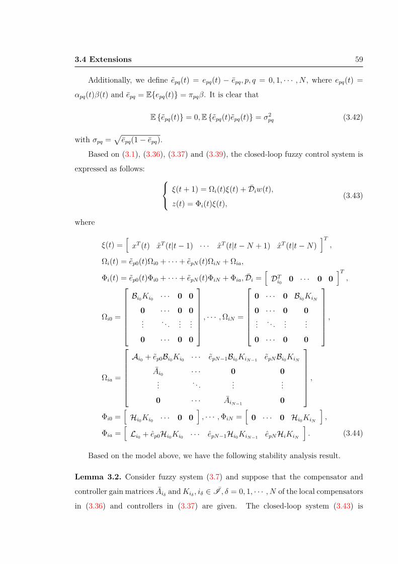
3.4 Extensions 59
Additionally, we define epq(t) = epq(t) − epq, p, q = 0, 1, · · · , N , where epq(t) =
αpq(t)β(t) and epq = Eepq(t) = πpqβ. It is clear that
E epq(t) = 0,E epq(t)epq(t) = σ2pq (3.42)
with σpq =√epq(1− epq).
Based on (3.1), (3.36), (3.37) and (3.39), the closed-loop fuzzy control system is
expressed as follows: ξ(t+ 1) = Ωi(t)ξ(t) + Diw(t),
z(t) = Φi(t)ξ(t),(3.43)
where
ξ(t) =[xT (t) xT (t|t− 1) · · · xT (t|t−N + 1) xT (t|t−N)
]T,
Ωi(t) = ep0(t)Ωi0 + · · ·+ epN(t)ΩiN + Ωia,
Φi(t) = ep0(t)Φi0 + · · ·+ epN(t)ΦiN + Φia, Di =[DT
i00 · · · 0 0
]T,
Ωi0 =
Bi0Ki0 · · · 0 0
0 · · · 0 0... . . . ... ...
0 · · · 0 0
, · · · ,ΩiN =
0 · · · 0 Bi0KiN
0 · · · 0 0... . . . ... ...
0 · · · 0 0
,
Ωia =
Ai0 + ep0Bi0Ki0 · · · epN−1Bi0KiN−1
epNBi0KiN
Ai0 · · · 0 0... . . . ... ...
0 · · · AiN−10
,
Φi0 =[Hi0Ki0 · · · 0 0
], · · · ,ΦiN =
[0 · · · 0 Hi0KiN
],
Φia =[Li0 + ep0Hi0Ki0 · · · epN−1Hi0KiN−1
epNHiKiN
]. (3.44)
Based on the model above, we have the following stability analysis result.
Lemma 3.2. Consider fuzzy system (3.7) and suppose that the compensator and
controller gain matrices Aiδ andKiδ , iδ ∈ I , δ = 0, 1, · · · , N of the local compensators
in (3.36) and controllers in (3.37) are given. The closed-loop system (3.43) is

3.4 Extensions 60
stochastically stable with guaranteed H∞ performance γ, if there exists a set of
matrices Xi0...iN−1iN = XTi0...iN−1iN
> 0, i0, · · · , iN−1, iN ∈ I satisfying:Λ1 0 Λ2Xi0...iN−1iN 0
∗ Λ3 Λ4Xi0...iN−1iN Λ5
∗ ∗ −Xi0...iN−1iN 0
∗ ∗ ∗ −I
< 0, i, s ∈ I , (3.45)
where
Λ1 = diag−γ2I, · · · ,−γ2I,−γ2I,Λ2 =[σp0Φ
Ti0 · · · σpNΦ
TiN ΦT
ia
]T,
Λ3 = diag−Xj0...jN−1jN , · · · ,−Xj0...jN−1jN ,−Xj0...jN−1jN,
Λ4 =[σp0Ω
Ti0 · · · σpNΩ
TiN ΩT
ia
]T,Λ5 =
[0 · · · 0 DT
i0
]T. (3.46)
Proof. The proof is omitted for its similarity to Lemma 3.1.
Remark 3.16. A piecewise quadratic Lyapunov function is also utilized in Lemma
3.2, which will reduce to the common quadratic Lyapunov function if Xi0...iN−1iN = X
for any i0, . . . , iN ∈ I in (3.45).
In terms of Lemma 3.2, now we present the controller synthesis result in the
following theorem.
Theorem 3.2. Consider fuzzy system (3.7). The closed-loop system (3.43) is
stochastically stable with guaranteed H∞ performance γ, if there exist matrices
Xi0...iN−1iN = XTi0...iN−1iN
> 0, Riδ , Qiδ , iδ ∈ I and G such that the following linear
matrix inequalities are satisfied for all δ, p = 0, 1, 2, · · · , N:Λ1 0 Λ2 0∗ Λ3 Λ4 Λ5
∗ ∗ Xi0...iN−1iN − G− GT 0
∗ ∗ ∗ −I
< 0,m ∈ ℵ(i0), i0, · · · , iN ∈ I ,
(3.47)

3.4 Extensions 61
where
G =
G · · · G G... . . . ... ...
G · · · G G
G · · · G G
, Dm =
Dm
...
00
,
Λ2 =
σp0Θmi0
...
σpNΘmiN
Θmia
, Λ4 =
σp0Ξmi0
...
σpNΞmiN
Ξmia
, Λ5 =
0...
0Dm
,
Ξmi0 =
BmQi0 · · · BmQi0 BmQi0
0 · · · 0 0... . . . ... ...
0 · · · 0 0
...
ΞmiN =
BmQiN · · · BmQiN BmQiN
0 · · · 0 0... . . . ... ...
0 · · · 0 0
,
Ξmia =
Ξmia(1) · · · Ξmia(1) Ξmia(1)
Ri0 · · · Ri0 Ri0
... . . . ... ...
RiN−1· · · RiN−1
RiN−1
,Ξmia(1) = AmG+ ep0BmQi0 + · · ·+ epNBmQiN ,
Θmi0 =[HmQi0 · · · HmQi0 HmQi0
]...
ΘmiN =[HmQiN · · · HmQiN HmQiN
],
Θmia =[Θpia(1) · · · Θpia(1) Θpia(1)
],
Θpia(1) = LpG+ em0HpQi0 + · · ·+ emNHpQiN . (3.48)
Moreover, the controller gains and the compensation matrices are respectively
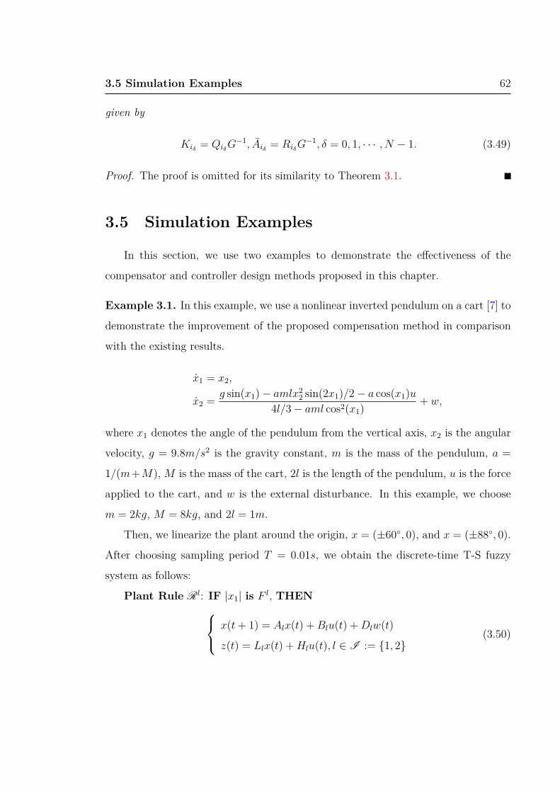
3.5 Simulation Examples 62
given by
Kiδ = QiδG−1, Aiδ = RiδG
−1, δ = 0, 1, · · · , N − 1. (3.49)
Proof. The proof is omitted for its similarity to Theorem 3.1.
3.5 Simulation Examples
In this section, we use two examples to demonstrate the effectiveness of the
compensator and controller design methods proposed in this chapter.
Example 3.1. In this example, we use a nonlinear inverted pendulum on a cart [7] to
demonstrate the improvement of the proposed compensation method in comparison
with the existing results.
x1 = x2,
x2 =g sin(x1)− amlx22 sin(2x1)/2− a cos(x1)u
4l/3− aml cos2(x1)+ w,
where x1 denotes the angle of the pendulum from the vertical axis, x2 is the angular
velocity, g = 9.8m/s2 is the gravity constant, m is the mass of the pendulum, a =
1/(m+M), M is the mass of the cart, 2l is the length of the pendulum, u is the force
applied to the cart, and w is the external disturbance. In this example, we choose
m = 2kg, M = 8kg, and 2l = 1m.
Then, we linearize the plant around the origin, x = (±60, 0), and x = (±88, 0).
After choosing sampling period T = 0.01s, we obtain the discrete-time T-S fuzzy
system as follows:
Plant Rule Rl: IF |x1| is F l, THEN x(t+ 1) = Alx(t) + Blu(t) +Dlw(t)
z(t) = Llx(t) +Hlu(t), l ∈ I := 1, 2(3.50)

3.5 Simulation Examples 63
0
0
0.2
0.4
0.6
0.8
1
|x1(t)|
µ
Rule1Rule2
π
18
π
3
S2
S1
(a) Membership functions of the system in (3.50)
0 50 100 150 200
0
0.5
1
Time in samples
α(t)
0 50 100 150 200
0
0.5
1
Time in samples
β(t)
(b) Data-packet dropout
0 50 100 150 2000
0.2
0.4
0.6
0.8
Time in samples
stat
e x 1(t
) tr
ajec
tory
Zero−StrategyHold−StrategyTheorem 3.2
0 50 100 150 200−2
−1
0
1
Time in samples
stat
e x 2(t
) tr
ajec
tory
Zero−StrategyHold−StrategyTheorem 3.2
(c) State responses
0 50 100 150 2000
0.002
0.004
0.006
0.008
0.01
0.012
0.014
0.016
0.018
0.02
Time in samples
Res
pons
e of
the
ratio
ζ
Zero−StrategyHold−StrategyTheorem 3.2
(d) Response of the ratio ζ
Figure 3.3: Simulation Results of Example 5.1
where
A1 =
1 0.01
0.1729 1
, B1 =
0
−0.0018
, D1 =
0
0.01
,A2 =
1 0.01
0.0585 1
, B2 =
0
−0.0007792
, D2 =
0
0.01
,L1 = L2 =
[0.5 0.1
], H1 = 0.005, H2 = 0.01.
The membership functions are shown in Fig.3.3(a). It is noted that the fuzzy
system is governed by one linear dynamic when 0 ≤ |x1| < π18
according to Fig.3.3(a),
and a fuzzy blending of two local dynamics when π18
≤ |x1| ≤ π3. Applying the
partition method given in the second section, the physical plant can be partitioned

3.5 Simulation Examples 64
into two regions, which are described as follows:
S1 := x|0 ≤ |x1| <π
18,
S2 := x| π18
≤ |x1| ≤π
3.
Similar to the case in the physical plant node, the states in the compensator and
controller nodes are partitioned into two regions as follows:
S1 := x|0 ≤ |x1| <π
18,
S2 := x| π18
≤ |x1| ≤π
3.
With such a partition, the fuzzy system is rewritten in each region as follows: x(t+ 1) = Aix(t) + Biu(t) +Diw(t)
z(t) = Lix(t) +Hiu(t), x(t) ∈ Si, i ∈ 1, 2,
where
A1 = A1,B1 = B1,D1 = D1,L1 = L1,H1 = H1,
A2 =2∑
m=1
µmAm,B2 =2∑
m=1
µmBm,D2 =2∑
m=1
µmDm,
L2 =2∑
m=1
µmLm,H2 =2∑
m=1
µmHm.
It is noted that the open-loop system is unstable. The objective is to design
a piecewise fuzzy compensator and state feedback controller of the form (3.10)
and (3.13) so that the closed-loop system (3.18) is stochastically stable with H∞
performance γ.
When α = 0.2 and β = 0.2, there are no feasible solutions utilizing the zero or
hold strategies, while we obtain γmin = 0.5551 by applying Theorem 3.1. The feasible
controller and compensator gains are
K1 =[−2.3634 0.8538
], K2 =
[−2.3633 0.8538
],
A1 = 10−3 ×
−0.0882 0.3245
−0.2131 0.7617
, A2 = 10−3 ×
−0.0852 0.3237
−0.2088 0.7608
.

3.5 Simulation Examples 65
Table 3.1: minimum H∞ performance γmin in each situation of Example 5.1
Models α/β 0/0 0.2/0.2 0.3/0.3 0.4/0.4 0.5/0.5 0.6/0.6 1/1
Zero-Strategy γmin ∞ ∞ 7.985 0.737 0.437 0.314 0.096
Hold-Strategy γmin ∞ ∞ ∞ 0.811 0.392 0.278 0.140
Theorem 3.1 γmin ∞ 0.555 0.368 0.287 0.240 0.208 0.135
With the purpose of illustrating the state responses, α = 0.4 and β = 0.4 are
assumed such that there are feasible solutions by different strategies. We assume the
initial conditions of the system to be x(0) = x(0) =[
π5
0]T
. The data missing
is randomly generated according to the probability shown in Fig.3.3(b). The state
responses are illustrated in Fig.3.3(c), where the external disturbance w(t) = 0. It
can be observed that the states of the closed-loop system converge to zero.
In order to illustrate the H∞ performance, we assume the initial conditions to
be zero, and the external disturbance w(t) = e−0.1t cos (2t). Fig.3.3(d) shows the
response of the ratio ζ of the closed-loop system, where ζ =√∑k
i=0 zT (i)z(i)√∑k
i=0 wT (i)w(i)
.
From Fig.3.3 we can observe that better H∞ performance and system response can
be achieved by the proposed compensation method in comparison with other strategies.
The more detailed comparison between the existing strategies and the
compensation strategy proposed in this chapter on the minimum H∞ performance
γmin under various scenarios of α and β is illustrated in Table 3.1, which clearly
demonstrates that much better H∞ performance can be achieved by utilizing the
proposed strategy than those existing ones.
Remark 3.17. It is noted from Table 3.1 that the proposed strategy does not achieve
the best system performance in the special case when α = β = 1, which implies that
there are no packet dropouts throughout the transmission. That is because the
compensator incurs some unnecessary effects in that special case. In this case, a
normal fuzzy controller would be used instead if there are no packet dropouts, which
can be found in some existing results, see [12] and references therein.
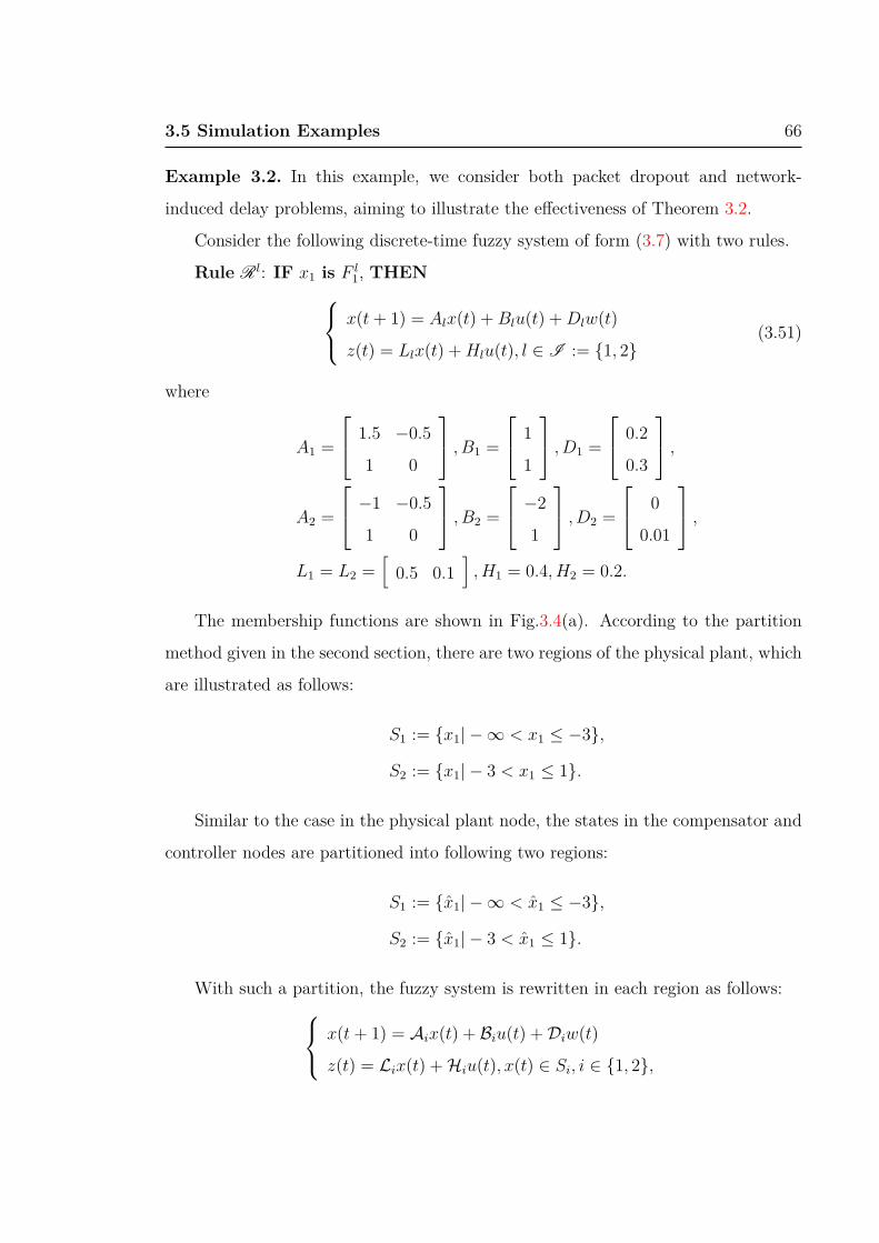
3.5 Simulation Examples 66
Example 3.2. In this example, we consider both packet dropout and network-
induced delay problems, aiming to illustrate the effectiveness of Theorem 3.2.
Consider the following discrete-time fuzzy system of form (3.7) with two rules.
Rule Rl: IF x1 is F l1, THEN x(t+ 1) = Alx(t) + Blu(t) +Dlw(t)
z(t) = Llx(t) +Hlu(t), l ∈ I := 1, 2(3.51)
where
A1 =
1.5 −0.5
1 0
, B1 =
1
1
, D1 =
0.2
0.3
,A2 =
−1 −0.5
1 0
, B2 =
−2
1
, D2 =
0
0.01
,L1 = L2 =
[0.5 0.1
], H1 = 0.4, H2 = 0.2.
The membership functions are shown in Fig.3.4(a). According to the partition
method given in the second section, there are two regions of the physical plant, which
are illustrated as follows:
S1 := x1| −∞ < x1 ≤ −3,
S2 := x1| − 3 < x1 ≤ 1.
Similar to the case in the physical plant node, the states in the compensator and
controller nodes are partitioned into following two regions:
S1 := x1| −∞ < x1 ≤ −3,
S2 := x1| − 3 < x1 ≤ 1.
With such a partition, the fuzzy system is rewritten in each region as follows: x(t+ 1) = Aix(t) + Biu(t) +Diw(t)
z(t) = Lix(t) +Hiu(t), x(t) ∈ Si, i ∈ 1, 2,

3.5 Simulation Examples 67
0
0.2
0.4
0.6
0.8
1
x1(t)
µ
Rule1Rule2
1−3
S2
S1
(a) Membership functions of the system in (3.51)
0 20 40 60 80 100
0
0.5
1
1.5
2
Time in samples
time
dela
y d(
t)
0 20 40 60 80 100
0
0.5
1
Time in samples
β(t)
(b) Network performance
0 20 40 60 80 100−2
−1
0
1
Time in samples
stat
e x 1(t
) tr
ajec
tory
0 20 40 60 80 100−0.4
−0.2
0
0.2
0.4
Time in samples
stat
e x 2(t
) tr
ajec
tory
(c) State responses
0 20 40 60 80 1000
0.02
0.04
0.06
0.08
0.1
0.12
Time in samples
Res
pons
e of
the
ratio
ζ
(d) Response of the ratio ζ
Figure 3.4: Simulation Results of Example 5.2
where
A1 = A1,B1 = B1,D1 = D1,L1 = L1,H1 = H1,
A2 =2∑
m=1
µmAm,B2 =2∑
m=1
µmBm,D2 =2∑
m=1
µmDm,
L2 =2∑
m=1
µmLm,H2 =2∑
m=1
µmHm.
In this example, the largest consecutive steps of network-induced delays and
packet dropouts N = 2 is assumed. Additionally, β = 0.95, and the transition

3.6 Conclusion 68
probability matrix is given by
T =
0.95 0.03 0.02
0.95 0.03 0.02
0.95 0.03 0.02
.By applying Theorem 3.2, the corresponding controller and compensation gains
are obtained as follows,
K1 =[−0.8153 0.1178
], K2 =
[−0.8117 0.0779
],
A1 = 10−3 ×
1.3262 −0.8298
1.6967 4.4351
, A2 = 10−3 ×
−0.5474 1.5152
−4.3911 5.9701
,and the minimum H∞ performance γmin = 0.2040. However, it is also noted that for
this example there is no feasible solution by utilizing the hold strategy.
To illustrate the closed-loop performance, some simulations have been done with
the initial conditions of the system as x(0) = x(0) =[−2 0
]T. The network-
induced delays and data missing are randomly generated according to the probability
shown in Fig.3.4(b). The state responses of the closed-loop system are illustrated in
Fig.3.4(c), where the external disturbance w(t) = 0. It can be observed that the
states of the closed-loop system converge to zero.
In order to illustrate the H∞ performance, we assume the initial conditions to
be zero, and the external disturbance w(t) = e−0.1t cos (2t). Fig.3.4(d) shows the
response of the ratio ζ of the closed-loop system.
From Fig.3.4 we can observe that the system is stochastically stable with
guaranteed H∞ performance, which shows the effectiveness of Theorem 3.2.
3.6 Conclusion
The H∞ control problem of fuzzy-model-based nonlinear NCSs with packet
dropouts is discussed in this chapter. A new compensation method for packet
dropouts is proposed, and a piecewise state feedback controller is designed. It is shown
that the closed-loop system is stochastically stable with guaranteed H∞ performance

3.6 Conclusion 69
with the existence of packet dropouts in both S/C and C/A channels. Moreover, the
proposed compensation method can achieve better control performance in comparison
to the existing approaches such as zero and hold strategies. Moreover, the results
are extended to the case where both packet dropouts and network-induced delay
phenomena exist. The developed results are illustrated by two simulation examples.

Chapter 4
H∞ Filter Design of Networked
Nonlinear Systems With
Communication Constraints via
T-S Fuzzy Dynamic Models
4.1 Introduction
In recent decades, great effort has been devoted to filter design in the field of
signal processing and control application. Among various filtering approaches, H∞
filter has attracted great attention because a guaranteed noise attenuation level can
be obtained without requiring the knowledge of noises a priori, and various theoretical
and application results have been published [129]- [130].
Generally, the current system output is needed in the H∞ filtering approach.
However, the measured output received by filter yF (t) is different from the current
system output y(t) under the network circumstance. Three typical problems of
network are quantization, delays and packet dropouts. Therefore, great attention
has been paid to the investigation of the filtering problem with communication
constraints, and many results have been reported [131]- [134]. To mention a few, the
authors in [131] study the H∞ filtering problem for networked discrete-time systems

4.1 Introduction 71
with random packet losses, which is described by a two-state Markov chain. The
authors in [132] consider the problem of state estimation for discrete-time dynamic
systems with quantized measurements, in which a logarithmic quantizer is utilized for
the quantization process. The authors in [133] investigate the problem of robust H∞
estimation for discrete-time systems subject to communication limitations including
measurement quantization, signal transmission delay, and packet dropout, in which
the three typical communication constraints are studied simultaneously.
It is noted that the considered plants are linear systems in all of the
aforementioned filtering results. However, most of the industrial plants have
nonlinear properties, so the filter design of nonlinear systems under the network
circumstance is desirable. As mentioned in Chapter 1, T-S fuzzy models can describe
some complex nonlinear systems by a group of local linear systems, which are blended
by several IF-THEN rules [14]- [15]. More recently, some results on the filtering
of fuzzy dynamic systems under the network circumstance have been reported.
However, most of them consider one or two aspects of the communication constraints.
To mention a few, the authors in [135] consider the H∞ filtering for nonlinear systems
with time-varying delay via T-S fuzzy model approach. [136] is concerned with H∞
filter design for fuzzy-model-based systems with transfer delays and packet loss. The
authors in [55] investigate the H∞ filtering for nonlinear discrete-time systems subject
to quantization and packet dropouts via T-S dynamic models. It is worth nothing that
few papers address the filter design problem of nonlinear systems with simultaneous
consideration of the three typical communication constraints mentioned previously,
which motivates our research.
In this chapter, we investigate the filter design of nonlinear systems subject to
those three important constraints of communication simultaneously. The nonlinear
physical plant is described by a T-S fuzzy model. By utilizing a piecewise Lyapunov
function method, the H∞ filter is obtained. Finally, an example is given to show the
effectiveness of our approach. The contributions of this chapter can be summarized
as follows: 1) a new approach to H∞ filtering is proposed, which considers three
communication constraints simultaneously for the nonlinear system via T-S dynamic

4.2 Model Description 72
Figure 4.1: Overall filtering error system
models; and 2) the proposed piecewise filter is based on piecewise quadratic Lyapunov
functions without obtaining the region information where the current system states
stay, which is more useful in application.
The remainder of the chapter is organized as follows. Section II is devoted to
problem formulation and the description of the novel filter design method. Section III
presents the H∞ filtering results based on a piecewise quadratic Lyapunov function.
In Section IV, a simulation example is given to illustrate the effectiveness of the
proposed approach. Finally, a conclusion is drawn in section V.
4.2 Model Description
In this chapter, we focus on a class of T-S fuzzy systems with communication
constraints as illustrated in Fig.4.2.
4.2.1 Physical Plant
The T-S fuzzy-model-based physical plant is given by:

4.2.1 Physical Plant 73
Plant Rule Rl: IF θ1(t) is F l1 and θ2(t) is F l
2 and · · · and θv(t) is F lv, THEN
x(t+ 1) = Alx(t) +Dlw(t)
z(t) = Llx(t) +Hlu(t)
y(t) = Clx(t), l ∈ I := 1, 2, ..., r,
(4.1)
where Rl denotes the lth fuzzy inference rule, r the number of inference rules, F lφ(φ =
1, 2, ..., v) the fuzzy sets, x(t) ∈ ℜnx the state vector, y(t) ∈ ℜnz the regulated output
vector, z(t) ∈ ℜnz the signal vector to be estimated, w(t) ∈ ℜnw the disturbance
input vector, [θ1(t), θ2(t), · · · , θv(t)] the premise variables, which are some measurable
variables of the system such as the state variables, and (Al, Cl, Dl, Ll, Hl) denotes the
matrices of the system’s lth local model.
By using a standard fuzzy inference method, which includes a singleton fuzzifier,
product fuzzy inference and center-average defuzzier, the T-S fuzzy system in (4.1)
can be rewritten as, x(t+ 1) = A(µ)x(t) +D(µ)w(t)
z(t) = L(µ)x(t) +H(µ)u(t)
y(t) = C(µ)x(t),
(4.2)
where
A(µ) =r∑
l=1
µlAl, D(µ) =r∑
l=1
µlDl, C(µ) =r∑
l=1
µlCl,
L(µ) =r∑
l=1
µlLl, H(µ) =r∑
l=1
µlHl, (4.3)
and µl is the normalized membership function satisfying
µl =ζl(θ)∑r
φ=1 ζφ(θ), ζl(θ) =
v∏φ=1
F lφ(θφ),
µl ≥ 0,r∑
l=1
µl = 1 (4.4)
with F lφ(θφ) representing the grade of membership of θφ in the fuzzy set F l
φ.
In order to investigate the robust H∞ filtering problem for system (4.1) based
on piecewise Lyapunov functions, the premise variable space is partitioned into a

4.2.2 Quantization, Encoding and Decoding 74
number of polyhedral regions Sii∈I ⊆ ℜv, which are divided into crisp and fuzzy
regions with the following definitions, respectively,
Sic = θ(t)|µm(θ(t)) = 1,m ∈ ℵ(ic), ic ∈ I , (4.5)
and
Sif = θ(t)|0 ≤ µm(θ(t)) < 1,m ∈ ℵ(if ), if ∈ I , (4.6)
where ℵ(ic),ℵ(if ) are sets containing the indices of rules in each region, and I is the
set of polyhedral regions.
With such a partition, the fuzzy system (4.2) is rewritten in each region asx(t+ 1) = Aix(t) +Diw(t)
z(t) = Lix(t) +Hiw(t)
y(t) = Cix(t), x(t) ∈ Si, i ∈ I ,
(4.7)
where
Ai =∑
m∈ℵ(i)
µmAm,Di =∑
m∈ℵ(i)
µmDm, Ci =∑
m∈ℵ(i)
µmCm,
Li =∑
m∈ℵ(i)
µmLm,Hi =∑
m∈ℵ(i)
µmHm, (4.8)
with 0 ≤ µm(θ(t)) ≤ 1,∑
m∈ℵ(i) µm(θ(t)) = 1.
In order to carry out the filter design based on piecewise Lyapunov functions, we
also define a set T that represents all possible transitions among regions as follows:
T :=(i, j)|θ(t) ∈ Si, θ(t+ 1) ∈ Sj,∀i, j ∈ I
. (4.9)
The states remain in the same region Si in the case of j = i, (i, j) ∈ T . Otherwise,
the states transit from region Si to Sj.
4.2.2 Quantization, Encoding and Decoding
Because of the limited bandwidth of communication links, data need to be
quantized and encoded at the sending node, while decoded at the receiving node.
There are numerous quantization approaches in the field of communication, however,

4.2.3 Communication Links 75
just a few of them are utilized for the filter design. A widely used quantization method
is logarithmic quantization [55]. The mathematical expression of the quantizer
is convenient for the filter design and controller synthesis. However, it has the
saturation problem. Moreover, the quantizer needs infinite network bandwidth when
the system near the equilibrium, which is unpractical in actual application.
Motivated by [137], we utilize the following dynamic quantizer:
qρ(v) = ρq
(v
ρ
), (4.10)
where ρ > 0 is the ”zoom” variable, and q(v) is a static quantizer satisfying
|q(v)− v| ≤ ∆, if |v| ≤M. (4.11)
Remark 4.1. The range of the dynamic quantizer in (4.10) is [−Mρ,Mρ], and
the quantization error is[−∆ρ, ∆ρ
]. Therefore, the saturation and deterioration of
performance near the equilibrium problems of many other quantization methods can
be solved by increasing and decreasing the ”zoom” variable ρ.
Remark 4.2. The exact form of the static quantizer q(v) considered in this chapter
is not specified, which means that any quantizer satisfying (4.11) can be utilized,
such as uniform quantization [39] and some non-uniform quantization methods.
It is noted that the measurement outputs need to be quantized by multiple
quantizers because the ranges of each output are different, which is denoted as follows:
q(v) =[q(1)Tρ1 (v1) q
(2)Tρ2 (v2) · · · q
(nv)Tρnv
(vnv)]T
= ∆q(v)N (4.12)
where vj is the jth component of v, q(j)ρj (vj) is a dynamic quantizer,
∆q(v) = diagq(1)ρ1 (v1), q
(2)ρ2 (v2), · · · , q
(nv)ρnv
(vnv)
, and N =[1 1 · · · 1
]T.
4.2.3 Communication Links
It is noted that packet dropout and network-induced delay phenomena exist in
the communication links. Therefore, the inputs to the filter yc(t) are not the same as
the outputs of the physical plant y(t).

4.2.4 Filter Error System 76
We assume that there exists a buffer in the filter node, which stores the received
historical data. Motivated by [138], we model the unreliable transmission as follows:
yc(t) = qρ(y(tτ )), (4.13)
where qρ(y(tτ )) denotes the latest data stored in the buffer of the filter node at
sampling time t. We use quantizers in (4.13) satisfying
qρ(y(tτ ))− y(tτ ) = ∆(y(tτ ))N, (4.14)
where ∆(y(tτ )) = diagq(1)ρ1 (y1(tτ )), · · · , q
(ny)ρny
(yny(tτ ))
with ∆(y(tτ )) ≤ ∆ = diagρ1M1, ρ2M2, · · · , ρnyMny
.
We define τ(t) = t − tτ , which is the time-delay of the packet in the filter node
caused by the network-induced delay and packet dropout phenomena.
The following assumption is needed on modeling the random time-delay in the
buffers caused by the unreliable transmission.
Assumption 4.1. The time-delay τ(t) is time varying and satisfy 0 ≤ τ1(t) ≤ τM ,
where τM represents the upper bound on the time-delay in the buffer.
4.2.4 Filter Error System
Based on the T-S fuzzy system in (4.7) in each region, we consider the following
piecewise filter. x(t+ 1) = Asx(t) +Rsyc(t),
z(t) = Lsx(t), s ∈ I(4.15)
where x(t) is the state vector of the filter, As, Ls, Rs, s ∈ I are filter matrices in each
local region to be determined.
For the filter state x(t), we also define a set T to describe the region transitions:
T =(s, k)|x(t) ∈ Ss, x(t+ 1) ∈ Sk, s, k ∈ I
. (4.16)
Remark 4.3. It is noted that the states of a physical plant are not always available
in the filter node due to the unreliable transmission. In this case, the plant states
and the filter states might not be in the same region, thus the region transitions of

4.2.5 Problem Formulation 77
the physical plant and filter might not be synchronized, which are defined in (4.9)
and (4.16), respectively. Therefore, the filter in (4.15) utilizes the gains according to
region of filter states.
Remark 4.4. It is noted from [127] that the filter will be identical to the linear filter
if we design a fuzzy filter based on conventional parallel distributed compensation
(PDC) [117] when the premise variables between the physical plant and the designed
fuzzy filter are different. Therefore, the piecewise filter in (4.15) is designed, which is
less conservative.
From (4.7), (4.13)-(4.15), we have the following filtering error dynamic system: ξ(t+ 1) = Aisξ(t) + Bshξ(t− τ(t)) + Diw(t) + Es,
e(t) = Lis(t)ξ(t) +Hiw(t), i, h, s ∈ I ,(4.17)
where
ξ(t) =[xT (t) xT (t)
]T,Lis =
[Li Ls
],
Es(t) =[
0 Rs∆(y(t− τ(t)))N],Di =
Di
0
T
,
Ais =
Ai 0
0 As
,Bsh =
0 0
−RsCh 0
. (4.18)
4.2.5 Problem Formulation
Before proceeding further, a basic definition is introduced as follows:
Definition 4.1. The filtering error system in (4.17) is said to be asymptotically
stable with an H∞ performance γ if it is asymptotically stable when w(t) = 0, and
satisfies
∥e∥2 ≤ γ∥w∥2, (4.19)
where ∥e∥2 :=√∑∞
t=0 eT (t)e(t), and γ > 0 is a prescribed scalar.
The problem to be addressed in this chapter is described as follows.

4.3 Main Results 78
H∞ Filter Design Problem. Consider the fuzzy system in (4.1). Design a
piecewise filter in the form of (4.15) such that the filtering error system (4.17) is
asymptotically stable with guaranteed H∞ performance γ.
Before presenting the main results, three lemmas are introduced as follows, which
will be utilized subsequently.
Lemma 4.1. [139] Given appropriately dimensioned matrices Ω1,Ω2, and Ω3 with
Ω1 = ΩT1 , then
Ω1 + Ω3Υ(k)Ω2 + ΩT2Υ
T (k)ΩT3 < 0 (4.20)
holds for all Υ(k) satisfying ΥT (k)Υ(k) ≤ I if and only if for some ε > 0
Ω1 + ε−1Ω3ΩT3 + εΩT
2Ω2 < 0 (4.21)
Lemma 4.2. [140] For any constant matrix M > 0, any scalars a and b with a < b,
the following inequation is satisfied:[b∑
i=a
x(i)
]TM
[b∑
i=a
x(i)
]≤ (b− a+ 1)
[b∑
i=a
xT (i)Mx(i)
]
(4.22)
Lemma 4.3. [55] For any constant matrix P > 0 and G, the following inequation
holds:
−GTP−1G ≤ P −G−GT (4.23)
4.3 Main Results
In this section, the piecewise filter design problem of the fuzzy system (4.1) is
investigated, which is solved by a linear matrix inequality (LMI) approach based on
piecewise Lyapunov functions.

4.3.1 Stability Analysis 79
4.3.1 Stability Analysis
The following lemma presents a condition to guarantee the stability and H∞
performance of the overall error system (4.17).
Theorem 4.1. Consider the system (4.1) and suppose that the filter matrices
As, Rs, Ls of the local filter in (4.15) are given. The overall error system (4.17)
is asymptotically stable with guaranteed H∞ performance γ, if there exist matrices
Pis = P Tis > 0, i, s ∈ I , Z, λ, g and ϵ satisfying
Πisjkh < 0, i, s, j, k, h ∈ I , (4.24)
where
Πisjkh =
Π11isjkh Π12
isjkh
∗ Π22isjkh
,Π11
isjkh = diag−Pis,−τ−1
M Z,−I, λ− g − gT,
Π12isjkh =
PjkΓ1 PjkBsh PjkDi 0 PjkΓ2
ZΓ3 ZBsh PjkDi 0 PjkΓ2
Lis 0 Hi 0 00 0 0 g 0
,Π22
isjkh = diag−Pjk,−τ−1
M Z,−γ2I,−λ+ ϵNTN,−ϵ,
Γ1 =
Ai 0RsCh As
,Γ2 =
0Rs∆
,Γ3 =
Ai − I 0RsCh As − I
. (4.25)
Proof. Consider the following piecewise Lyapunov function,
V (t) = V1 + V2, (4.26)
where
V1 = ξT (t)Pisξ(t), i, s ∈ I ,
V2 =−1∑
q=−τM
t−1∑p=t+q
ξT (p)Zξ(p), (4.27)
with P Tis = Pis > 0, Z are Lyapunov matrices to be determined, and ξ(t) = ξ(t+1)−
ξ(t).

4.3.1 Stability Analysis 80
It is known that the error system in (4.17) can be demonstrated as asymptotically
stable with H∞ performance γ under zero initial conditions by proving the following
index J is negative:
J = V (t+ 1) + γ−2zT (t)z(t)− V (t)− wT (t)w(t). (4.28)
From (4.17) and Lemma 4.2, we have
J ≤ ξT (t+ 1)Pjkξ(t+ 1)− ξT (t)XPisξ(t) + eT (t)e(t)− γ2wT (t)w(t)
+τM ξT (t)Zξ(t)− τ−1
M
t−1∑p=t−τ(t)
ξT (p)Zt−1∑
p=t−τ(t)
ξ(p) + λ− λ
= ηT (t)ΘTdiag Pjk, τMZ, I, λΘη(t)
+ηT (t)diag−Pis,−τ−1
M Z,−γ2I,−λη(t), (4.29)
where
η =[ξT (t)
∑t−1p=t−τ(t) ξ
T (p) wT (t) 1]T,
Θ =
Γ1 Bsh Di Es(t)
Γ3 Bsh Di Es(t)
Lis 0 Hi 0
0 0 0 1
, (4.30)
Then by the Schur complement, Lemma 4.1, Lemma 4.3 and (4.24), we have J < 0.
The proof is thus completed.
Remark 4.5. In order to achieve less conservative results, a piecewise quadratic
Lyapunov functional method is utilized in this work [141]. It is noted that common
quadratic Lyapunov function is a special case of the piecewise Lyapunov function
when the same Lyapunov function is utilized in different partitions. Another typical
less conservative Lyapunov function used in T-S fuzzy control is fuzzy Lyapunov
function, but it will be identical to the common Lyapunov function if the premise
variables of the physical plant and those of the designed fuzzy filter are different [127].
Obviously, (4.27) will reduce to the common quadratic Lyapunov function if Xis = X
for any i, s ∈ I .

4.3.2 Filter Design 81
4.3.2 Filter Design
In terms of Lemma 4.1, now we present the filter design result.
Theorem 4.2. Consider the system (4.1). The overall error system (4.17) is
asymptotically stable with guaranteed H∞ performance γ, if there exist matrices
Pis = P Tis > 0, Gs, Rs, Qs, i, s ∈ I , Z, λ, g and ϵ satisfying
Πisjkmn < 0, i, s, j, k ∈ I ,m ∈ ℵ(i), n ∈ ℵ(h), (4.31)
where
Πisjkmn =
Π11isjkmn Π12
isjkmn
∗ Π22isjkmn
,Π11
isjkmn = diagPis −Gs −GT
s , τMZ −Gs −GTs ,−I, λ− g − gT
,
Π12isjkmn =
Γ1 Γ4 Dm 0 Γ2
Γ3 Γ4 Dm 0 Γ2
Γ5 0 Hm 0 00 0 0 g 0
,Π22
isjkmn = diag−Pjk,−τ−1
M Z,−γ2I,−λ+ ϵNTN,−ϵ,
Gs =
Gs1 Gs2
Gs3 Gs2
, Γ1 =
Gs1Am + RsCn Qs
Gs3Am + RsCn Qs
, Γ2 =
Rs∆
Rs∆
,Γ3 =
Gs1(Am − I) + RsCn Qs −Gs2
Gs3Am + RsCn Qs −Gs2
, Γ4 =
−RsCn 0−RsCn 0
Γ5 =
[Lm −Ls
], Dm =
[DT
m DTm
]T. (4.32)
Moreover, the filter matrices are respectively given by
As = G−1s2 Qs, Rs = G−1
s2 Rs, s ∈ I . (4.33)
Proof. Based on (4.8), the left hand side of (4.24) can be rewritten as

4.4 Simulation Example 82∑m∈ℵ(i)
∑n∈ℵ(h) µmµnΠisjkmn, i, s, j, k ∈ I , where
Πisjkmn =
Π11isjkh Π12
isjkmn
∗ Π22isjkh
,
Π12isjkmn =
PjkΓ1 PjkBsn PjkDm 0 PjkΓ2
ZΓ3 ZBsn PjkDm 0 PjkΓ2
Lms 0 Hm 0 0
0 0 0 g 0
,
Γ1 =
Am 0
RsCn As
, Bsn =
0 0
−RsCn 0
,Γ3 =
Am − I 0
RsCn As − I
, Lms =[Lm −Ls
]. (4.34)
Then, post- and pre-multiplying Πisjkmn by diagGsP
−1jk , GsZ
−1, I, I, I, I, I, I, I
and its transpose, respectively. It is noted from Lemma 4.3 that (4.31) yields (4.24),
and the proof is thus completed.
4.4 Simulation Example
In this section, we use an example to demonstrate the effectiveness of the filter
design method proposed in this chapter.
Example 4.1. In this example, we use the discrete-time T-S fuzzy system as follows:
Plant Rule Rl: IF x1 is F l, THENx(t+ 1) = Alx(t) +Dlw(t)
z(t) = Llx(t) +Hlw(t)
y(t) = Cl, l ∈ I := 1, 2
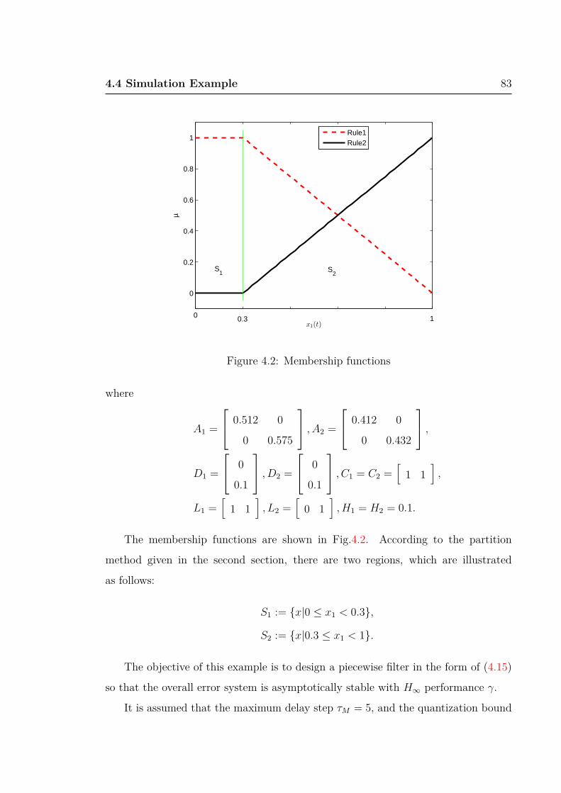
4.4 Simulation Example 83
0
0
0.2
0.4
0.6
0.8
1
x1(t)
µ
Rule1Rule2
0.3 1
S2
S1
Figure 4.2: Membership functions
where
A1 =
0.512 0
0 0.575
, A2 =
0.412 0
0 0.432
,D1 =
0
0.1
, D2 =
0
0.1
, C1 = C2 =[1 1
],
L1 =[1 1
], L2 =
[0 1
], H1 = H2 = 0.1.
The membership functions are shown in Fig.4.2. According to the partition
method given in the second section, there are two regions, which are illustrated
as follows:
S1 := x|0 ≤ x1 < 0.3,
S2 := x|0.3 ≤ x1 < 1.
The objective of this example is to design a piecewise filter in the form of (4.15)
so that the overall error system is asymptotically stable with H∞ performance γ.
It is assumed that the maximum delay step τM = 5, and the quantization bound

4.4 Simulation Example 84
0 50 100 150 200−0.2
0
0.2
0.4
0.6
0.8
1
1.2
Time in samples
filte
ring
erro
r e(
t)
Figure 4.3: Filtering error
∆ = 4. By utilizing Theorem 4.1, we obtain the following filter matrices:
A1 =
0.408 −0.016
−0.021 0.418
, L1 =[−0.060 −0.194
],
A2 =
0.398 −0.015
−0.020 0.409
, L2 =[−0.048 −0.178
],
R1 = 10−14 ×
−0.134
−0.641
, R2 = 10−14 ×
−0.109
−0.758
with the minimum H∞ performance γmin = 0.2288.
The following disturbance w(t) is assumed
w(t) = e−0.1tcos(2t),
and the simulation results of the filtering error is shown in Fig.4.3. By calculation,
we have ∥w(t)∥22 = 2.0384, ∥e(t)∥22 = 0.0786, which yields√∥e(t)∥22∥w(t)∥22
= 0.1964 < γmin = 0.2288
showing the effectiveness of the H∞ filter design method.

4.5 Conclusion 85
4.5 Conclusion
The H∞ filtering problem of fuzzy-model-based nonlinear systems with
communication constraints is discussed in this chapter. A filter design method under
unreliable transmission is proposed, which considers quantization, network-induced
delays and packet dropouts simultaneously. It is shown that the filtering error system
is asymptotically stable with guaranteed H∞ performance. The developed results are
illustrated by a simulation example.

Chapter 5
Fuzzy Modeling and Control of A
Nonlinear Quadrotor Under
Network Environment
5.1 Introduction
In recent decades, great effort has been devoted to the control of quadrotor
aircrafts [142]- [144]. A quadrotor is a kind of Unmanned Aerial Vehicle (UAV) with
four propeller units which located in four symmetrical positions. They are able to
take off and land vertically without any airstrip, and they can hover in the air without
difficulties. All these features have attracted great research attention because of their
theoretical and practical significance, and they are applied in virous situations, such
as aerial photography, searching and rescuing people, forest fire detection and so
on [145].
Most of the existing results on the quadrotor are based on the traditional point-
to-point systems, where the sensors, controller and actuators are connected by wires
directly so that the actuators can update the control signals once the controller
obtains the information from the sensors and computes the control signals [143].
However, this is not true in actual applications, because the sensor information
are often delayed due to the procedure of measuring, sampling and transmitting.

5.1 Introduction 87
On the other hand, the embedded microprocessor utilized in the quadrotor is not
able to compute the control signals fast enough especially when some complex
control algorithms are implemented. Due to the huge computation and the limited
computational ability on the quadrotor aircraft, the computation time should be
considered. Additionally, the components of a quadrotor are often with an embedded
communication fieldbus [146], such as CAN network, which indicates the unperfect
transmission among the different nodes. Therefore, the control of network-based
systems is involved, which shows the great significance in practical situations [29].
In the meantime, the quadrotor dynamic is nonlinear, which makes it difficult
to design the corresponding controller to stabilize the quadrotor. However, most
of the existing results model the quadrotor system as a linear one, and design the
corresponding controller based on the linearized model [147]- [148]. The authors
in [149] utilize the conventional PID strategy to stabilize the quadrotor aircraft. It is
noted from Chapter 1 that T-S fuzzy models provide a powerful method for systematic
stability analysis and synthesis of some nonlinear systems [11]. It is proved that T-
S fuzzy systems are capable to approximate any smooth nonlinear system to any
accuracy on a compact set [12].
To our best knowledge, there are few results considering the nonlinear controller
design method of a nonlinear quadrotor under network environment, which motivates
our current research. In this chapter, we propose a novel analysis and synthesis
method of the network-based quadrotor aircraft. The controlled quadrotor is
approximiated by a T-S fuzzy model, and the corresponding fuzzy controller is
designed so that the overall system is asymptotically stable with guaranteed H∞
performance. Finally, a simulation is given to illustrate the effectiveness of our
method. The contribution of this chapter can be summarized as follows: 1) A
fuzzy modeling and fuzzy controller design method for the quadrotor under network
environment is proposed. 2) The delays caused by computation and the network are
considered.
The remainder of the chapter is organized as follows. Section II is devoted to
model description and problem formulation. Section III presents the H∞ analysis

5.2 Model Description and Problem Formulation 88
Figure 5.1: Photo of the quadrotor
and synthesis results based on a common quadratic Lyapunov function. In Section
IV, a simulation is given to illustrate the effectiveness of the proposed approaches.
Finally, a conclusion is drawn in section V.
5.2 Model Description and Problem Formulation
In this chapter, we focus on the attitude modeling and control of a nonlinear
quadrotor under network environment, which is shown in Fig.5.1. Fig.5.2 illustrates
the system structure. It is noted that the delays and packet dropouts exist both in
S/C and C/A channels. Additionally, the delays caused by the computation of the
control unit are also considered. Therefore, the inputs to the controller xc(t) are not
the same as the states of the controlled aircraft x(t) at time instant t, and the control
inputs to the aircraft u(t) are also different from the outputs of the controller uc(t).
Now, we model the quadrotor aircraft and controller mathematically.

5.2.1 Description of the quadrotor 89
Figure 5.2: Structure of the quadrotor system
5.2.1 Description of the quadrotor
The attitude of the controlled quadrotor aircraft has three degrees of freedom
(3DOF). The quadrotor is able to move in roll, pitch and yaw freely by changing the
speed of the four symmetrically located propellers. The intelligent sensors installed in
the platform can measure the three axes ϕ, θ, ψ of the aircraft and obtain the angular
velocities ϕ, θ, ψ by differentiation. The nonlinear model of the quandrotor aircraft
considered in this chapter can be given as follows [143]:ϕ(t) = θψ
(Iy−IxIx
)+ Jr
IxθΩ + u1 + d1w(t)
θ(t) = ϕψ(
Iz−IxIy
)− Jr
IyϕΩ + u2 + d2w(t)
ψ(t) = ϕθ(
Ix−IyIz
)+ u3 + d3w(t)
(5.1)
where
Ω = Kv(−V2 − V4 + V1 + V3)
u1 =blK2
v (V22 − V 2
4 )
Ix, u2 =
blK2v (V
23 − V 2
1 )
Iy
u3 =blK2
v (V21 − V 2
2 + V 23 − V 2
4 )
Iz(5.2)
ϕ, θ, ψ denote the roll angle, pitch angle and yaw angle, respectively. w(t) is
the disturbance input vector. Vi is the voltage applied to propeller i, Kv is the
transformation constant, Jr is the rotator inertia, Ix, Iy, Iz are the inertia X, Y, Z
axis, respectively. b denotes thrust coefficient, and l is the distance from pivot to
motor.

5.2.1 Description of the quadrotor 90
We define the state vector as x = [ϕ, θ, ψ, ϕ, θ, ψ]T and the control input vector
as u = [u1, u2, u3]T . Then, the nonlinear dynamic (5.1) can be rewritten as x(t) = A(t)x(t) + Bu(t) +Dw(t)
z(t) = Cx(t) +Hw(t),(5.3)
where
A(t) =
0 IrIxΩ Iyzxx3 0 0 0
−JrIxΩ 0 Ixyzx1 0 0 0
0 Ixyzx1 0 0 0 0
1 0 0 0 0 0
0 1 0 0 0 0
0 0 1 0 0 0
,
B =
I3×3
03×3
, D =
D
03×1
, H =[
E3×1
],
C =[
03×3 I3×3
], D =
[d1 d2 d3
]T. (5.4)
It is noted that there are three nonlinear terms in the matrix A(t), which are
Ω, x1(t), x3(t). Each of these terms is bounded due to the bounded attitude angles
and input voltage to the propellers. Therefore, the nonlinear dynamic (5.3) can
be approximated by a T-S fuzzy dynamic model. The following sector nonlinearity
approach [150] is utilized.
The term Ω is bounded by [Ωmin,Ωmax] with Ωmin = 4KvVmin and Ωmax = 4KvVmax
according to (5.2). Then the weighting function of Ω can be chosen as
w1 =Ωmax − Ω(t)
Ωmax − Ωmin(5.5)
The term Ω can be rewritten as Ω(t) = w1Ωmin + (1 − w1)Ωmax. It is noted that
0 ≤ w1 ≤ 1.
Similarly, we have x1(t) = w2x1 + (1 − w2)x1 and x3(t) = w3x3 + (1 − w3)x3,

5.2.1 Description of the quadrotor 91
where
w2 =x1 − x1(t)
x1 − x1, w3 =
x3 − x3(t)
x3 − x3,
x1 = x3 = ϕmax = ψmax = αmax,
x1 = x3 = ϕmin = ψmin = αmin. (5.6)
Then we can rewrite the nonlinear dynamic in (5.3) as the following T-S fuzzy
model x(t) =∑8
l=1 µlAlx(t) +Bu(t) +Dw(t)
z(t) = Cx(t) +Hw(t),(5.7)
where
µ1 = w1(1− w2)(1− w3), µ2 = w1w2w3,
µ3 = w1(1− w2)w3, µ4 = w1w2(1− w3),
µ5 = (1− w1)(1− w2)(1− w3),
µ6 = (1− w1)w2w3,
µ7 = (1− w1)(1− w2)w3,
µ8 = (1− w1)w2(1− w3),
and
A1 =
0 IrIxΩmin Iyzxx3 0 0 0
−JrIxΩmin 0 Izxyx1 0 0 0
0 Ixyzx1 0 0 0 0
1 0 0 0 0 0
0 1 0 0 0 0
0 0 1 0 0 0
.
The expression of the corresponding Al, l = 2, ..., 8 can be obtained similarly, and
they are omitted for the limited space.
Remark 5.1. In fact, the fuzzy dynamic of the physical quadrotor aircraft (5.7) is
nonlinear due to the nonlinearity of the membership functions µl. Additionally, this
model will reduce to the existing linear one if we choose Al = A for all l = 1, ..., 8,

5.2.2 Communication 92
which can be found in [148]. Therefore, the existing linear model is the special case
of the proposed fuzzy model, which means that the proposed model is more general.
5.2.2 Communication
It is noted that the physical quadrotor dynamic is continuous-time. However,
the system state has to be sampled periodically in order to be transmitted to the
controller through the network. It is assumed the sampling period is T . Considering
the time-delay and packet dropout phenomena in both S/C and C/A channels, we
have the following expression
xc(t) = x(kT − η1(t))
= x(t− τ(t)− η1(t)),
u(t) = uc(t− τc − η2(t)), t ∈ [kT, (k + 1)T ) , (5.8)
where τ(t) = t − kT , and τc is the calculation time of the controller unit. η1(t)
and η2(t) are delays in the buffer of controller and actuator nodes caused by the
network-induced delay and packet dropout, respectively.
Remark 5.2. There are memories in the controller and actuator nodes, which can
store the latest received packet from the sending node. If there are network-induced
delays and/or packet dropouts, the latest packet stored in the buffer will be utilized
for the computation. Therefore, we are able to treat network-induced delays, packet
dropouts and the packets out of sequence in this unified model simultaneously.
It is standard to have the following assumption.
Assumption 5.1. The total time-delay η(t) throughout the overall system is
bounded, that is, 0 ≤ η(t) ≤ η, where η(t) = τ(t) + η1(t) + τc + η2(t).

5.2.3 Controller 93
5.2.3 Controller
In this chapter, the following fuzzy state feedback controller is considered based
on the fuzzy model given in (5.7).
uc(t) =8∑
j=1
µηjKjxc(t), (5.9)
where Kl are controller gains of each subsystem to be determined.
Remark 5.3. Similar to the fuzzy modeling method, the controller (5.9) is also
nonlinear because of the nonlinearity of µj, j = 1, ..., 8. It will reduce to the linear
controller as most of the existing results if Kj = K.
5.2.4 Closed-loop System
The closed-loop system is written as follows based on (5.7)-(5.9), x(t) =∑8
l=1 µlAlx(t) +∑8
j=1 µηjBKjx(t− η(t)) +Dw(t),
z(t) = Cx(t) +Hw(t)(5.10)
5.2.5 Problem Formulation
In order to present the main results, we have the following definition:
Definition 5.1. [151] The closed-loop fuzzy system (5.10) is called asymptotically
stable with guaranteed H∞ performance γ if the system is asymptotically stable when
w(t) = 0, and satisfies ∫ ∞
0
∥z(t)∥2dt ≤ γ2∫ ∞
0
∥w(t)∥2dt, (5.11)
where ∥z(t)∥2 = zT (t)z(t), ∥w(t)∥2 = wT (t)w(t), and γ > 0 is a prescribed scalar.
The problem addressed in this chapter can be described as follows.
H∞ Fuzzy State Feedback Controller Design Problem. Consider the fuzzy
dynamic of the quadrotor aircraft in (5.7). Design a fuzzy controller in the form of
(5.9) so that the closed-loop system (5.10) is asymptotically stable with guaranteed
H∞ performance γ by Definition 5.1.

5.3 Main Results 94
5.3 Main Results
In this section, analysis and synthesis of the fuzzy dynamic model of the quadrotor
aircraft in (5.7) is investigated, which is solved by a linear matrix inequality (LMI)
technique based on common Lyapunov function.
Firstly, we have the following analysis lemma.
Lemma 5.1. Consider the fuzzy system (5.7), and it is supposed that the controller
gain matrices Kj of the controller (5.9) are given. The closed-loop system (5.10)
is asymptotically stable with guaranteed H∞ performance γ if there exist matrices
P = P T > 0, Q = QT > 0, R = RT > 0, L1, L2,M,N satisfyingΓlj + Ξ + ΞT √
ηM√ηN C
∗ −R 0 0
∗ ∗ −R 0
∗ ∗ ∗ −γ2I
< 0, (5.12)
where
Γlj =
Π11 Π12 L2BKj 0 L2D
∗ Π22 L1BKj 0 L1D
∗ ∗ 0 0 0
∗ ∗ ∗ −Q 0
∗ ∗ ∗ ∗ −1
,
Ξ =[N 0 M −N −M 0
],C =
[C 0 0 0 H
]T,
Π11 = Q+ L2Al + ATl L
T2 ,Π12 = P − L2 + AT
l LT1 ,
Π22 = ηR− L1 − LT1 . (5.13)
Proof. Consider the following common Lyapunov functional candidate,
V (t) = V1(t) + V2(t) + V3(t), (5.14)

5.3 Main Results 95
where
V1(t) = xT (t)Px(t),
V2(t) =
∫ t
t−η
xT (s)Qx(s)ds,
V3(t) =
∫ 0
−η
∫ t
t+β
xT (s)Rx(s)dsdβ, (5.15)
P = P T > 0, Q = QT > 0, R = RT > 0 are Lyapunov matrices to be determined.
It is noted that the closed-loop system (5.10) can be demonstrated asymptotically
stable with an H∞ performance γ by proving the following index J is negative,
J = V (t) + γ−2zT (t)z(t)− wT (t)w(t). (5.16)
Differentiating V (t), we have
V1(t) = 2xT (t)Px(t),
V2(t) = xT (t)Qx(t)− xT (t− η)Qx(t− η),
V3(t) = ηxT (t)Rx(t)−∫ t
t−η
xT (s)Rx(s)ds
= ηxT (t)Rx(t)−∫ t−η(t)
t−η
xT (s)Rx(s)ds−∫ t
t−η(t)
xT (s)Rx(s)ds
≤ ηxT (t)Rx(t) + ξT (t)MR−1MT ξ(t) + 2ξT (t)M [x(t− η(t))− x(t− η)]
+ξT (t)NR−1NT ξ(t) + 2ξT (t)N [x(t)− x(t− η(t))] , (5.17)
where
M =[MT
1 MT2 MT
3 MT4 MT
5
]T,
N =[NT
1 NT2 NT
3 NT4 NT
5
]T,
ξ(t) =[xT (t) xT (t) xT (t− η(t)) xT (t− η) wT (t)
]T(5.18)
It is obvious that the following equation holds for any appropriate dimensioned
L1 and L2
Φ ,[xT (t)L1 + xTL2
][x(t) + Alx(t) +BKj(t− η(t)) +Dw(t)]
≡ 0 (5.19)

5.3 Main Results 96
Then we have the following inequation based on (5.17)-(5.19)
J ≤ 2xT (t)Px(t) + xT (t)Qx(t)− xT (t− η)Qx(t− η)
+ηxT (t)Rx(t) + ξT (t)MR−1MT ξ(t) + ξT (t)NR−1NT ξ(t)
+2ξT (t)M [x(t− η(t))− x(t− η)] + 2ξT (t)N [x(t)− x(t− η(t))]
+2Φ + γ−2zT (t)z(t)− wT (t)w(t) (5.20)
It is noted that (5.12) yields J < 0 in consideration of the Schur component
lemma. Thus the proof is completed.
In terms of Lemma 5.1, we present the controller design method for the quadrotor
aircraft by the following theorem now.
Theorem 5.1. Consider the fuzzy dynamic model (5.7). The closed-loop system
(5.10) is asymptotically stable with guaranteed H∞ performance γ if there exist
matrices P = P T > 0, Q = QT > 0, R = RT > 0, L(1), L(2),M,N, K so that the
following linear matrix inequations are satisfied:
Ψlj =
Γlj + Ξ + ΞT √
ηM√ηN C
∗ −R 0 0∗ ∗ −R 0∗ ∗ ∗ −γ2I
< 0, (5.21)
where
Γlj =
Π11 Π12 Kj 0 LD
∗ Π22 Kj 0 LD
∗ ∗ 0 0 0∗ ∗ ∗ −Q 0∗ ∗ ∗ ∗ −1
,
Π11 = Q+ LAl + ATl L
T , Π12 = P − L+ ATl L
T , Π22 = ηR− L− LT ,
Kj =
Kj
Kj
, L =
L(1) LT(1)
L(1) L(2)
. (5.22)
Moreover, the controller gain matrices are given by
Kj = L−1(1)Kj (5.23)

5.3 Main Results 97
Proof. It is noted from (5.4) that
B =
I3×3
03×3
, (5.24)
so we have
LBKj =
L(1) LT(1)
L(1) L(2)
I3×3
03×3
Kj =
L(1)
L(1)
Kj =
L(1)Kj
L(1)Kj
,
Kj
Kj
. (5.25)
If we define L1 = L2 = L, then it is obvious that (5.21) yields (5.12), which indicates
the stability of the closed-loop system according to Lemma 5.1. The proof is thus
completed.
The result of Theorem 5.1 can be improved by the following theorem.
Theorem 5.2. Consider the fuzzy dynamic model (5.7). The closed-loop system
(5.10) is asymptotically stable with guaranteed H∞ performance γ if there exist
matrices P = P T > 0, Q = QT > 0, R = RT > 0, L(1), L(2),M,N, K so that the
following linear matrix inequations are satisfied:
Ψll < 0, l = 1, ..., 8,
Ψlj +Ψjl < 0, l < j, (5.26)
where Ψlj are defined in (5.21)
Proof. It is noted from (5.21) that
8∑l=1
8∑j=1
µlµηjΨlj =
8∑l=1
µlµηl Ψll +
7∑l=1
8∑j=l+1
µlµηj (Ψlj +Ψjl). (5.27)
Then we have Ψlj < 0 if (5.26) is satisfied. Therefore, (5.26) yields (5.21), which
guaranteed the stability of the closed-loop system (5.10). Thus the proof of Theorem
5.2 is completed.

5.4 Simulation 98
5.4 Simulation
In this section, we use the simulation results of the attitude control of the
quadrotor aircraft to demonstrate the effectiveness of the fuzzy modeling and control
method proposed in this chapter.
We extract the parameters of the quadrotor from [144], which are shown as
follows:
Vi ∈ [−10V, 10V],
Kv = 54.945 rad s/V,
Jr = 6 · 10−5 kgm2,
Ix = 0.0552 kgm2,
Iy = 0.0552 kgm2,
Iz = 0.1104 kgm2,
b = 3.935139× 10⁻⁶ N/Volt,
l = 0.1969 m,
T = 0.005 s,
ϕmin = θmin = ψmin = −π/4 rad/s,
ϕmax = θmax = ψmax = π/4 rad/s,
ϕmax = θmax = π/2 rad/s, ψmax = π rad/s.
The objective of this simulation is to approximate the nonlinear quadrotor aircraft
and then design a corresponding fuzzy controller so that the closed-loop system is
asymptotically stable with H∞ performance γ.
Firstly, we have the following fuzzy system according to the approximation
method presented in Section II x(t) =∑8
l=1 µlAlx(t) +Bu(t) +Dw(t)
z(t) = Cx(t) +Hw(t),
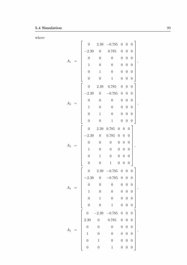
5.4 Simulation 99
where
A1 =
0 2.39 −0.785 0 0 0
−2.39 0 0.785 0 0 0
0 0 0 0 0 0
1 0 0 0 0 0
0 1 0 0 0 0
0 0 1 0 0 0
,
A2 =
0 2.39 0.785 0 0 0
−2.39 0 −0.785 0 0 0
0 0 0 0 0 0
1 0 0 0 0 0
0 1 0 0 0 0
0 0 1 0 0 0
,
A3 =
0 2.39 0.785 0 0 0
−2.39 0 0.785 0 0 0
0 0 0 0 0 0
1 0 0 0 0 0
0 1 0 0 0 0
0 0 1 0 0 0
,
A4 =
0 2.39 −0.785 0 0 0
−2.39 0 −0.785 0 0 0
0 0 0 0 0 0
1 0 0 0 0 0
0 1 0 0 0 0
0 0 1 0 0 0
,
A5 =
0 −2.39 −0.785 0 0 0
2.39 0 0.785 0 0 0
0 0 0 0 0 0
1 0 0 0 0 0
0 1 0 0 0 0
0 0 1 0 0 0
,
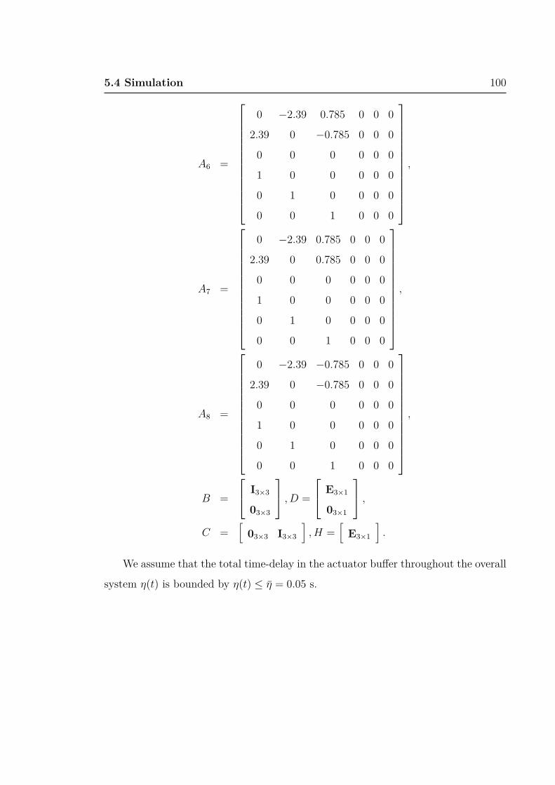
5.4 Simulation 100
A6 =
0 −2.39 0.785 0 0 0
2.39 0 −0.785 0 0 0
0 0 0 0 0 0
1 0 0 0 0 0
0 1 0 0 0 0
0 0 1 0 0 0
,
A7 =
0 −2.39 0.785 0 0 0
2.39 0 0.785 0 0 0
0 0 0 0 0 0
1 0 0 0 0 0
0 1 0 0 0 0
0 0 1 0 0 0
,
A8 =
0 −2.39 −0.785 0 0 0
2.39 0 −0.785 0 0 0
0 0 0 0 0 0
1 0 0 0 0 0
0 1 0 0 0 0
0 0 1 0 0 0
,
B =
I3×3
03×3
, D =
E3×1
03×1
,C =
[03×3 I3×3
], H =
[E3×1
].
We assume that the total time-delay in the actuator buffer throughout the overall
system η(t) is bounded by η(t) ≤ η = 0.05 s.

5.4 Simulation 101
0 0.5 1 1.5 2 2.5 3 3.5 4 4.50
0.005
0.01
0.015
0.02
0.025
0.03
0.035
0.04
0.045
0.05
Figure 5.3: Delays in the buffer
0 0.5 1 1.5 2 2.5 3 3.5 4 4.5−0.05
0
0.05
0.1
0.15
0.2
0.25
0.3
0.35
0.4
Time in seconds
angl
e
φθψ
Figure 5.4: Response

5.4 Simulation 102
Then by utilizing Theorem 5.2, we obtain the following controller gain matrices:
K1 =
−5.20 −2.74 1.31 −4.66 −1.96 −0.53
1.58 −5.17 0.05 −1.86 −4.65 −0.76
−0.76 −0.76 −3.89 −2.02 −2.03 −3.63
K2 =
−5.18 −2.72 −0.25 −4.67 −1.97 −0.45
1.55 −5.19 1.60 −1.85 −4.63 −0.84
−0.76 −0.76 −3.89 −2.03 −2.03 −3.63
K3 =
−5.18 −2.72 −0.25 −4.67 −1.97 −0.45
1.57 −5.17 0.05 −1.86 −4.64 −0.76
−0.76 −0.76 −3.89 −2.03 −2.03 −3.63
K4 =
−5.20 −2.74 1.30 −4.66 −1.96 −0.53
1.55 −5.19 1.60 −1.85 −4.63 −0.84
−0.76 −0.76 −3.89 −2.03 −2.03 −3.63
K5 =
−5.19 1.55 1.60 −4.63 −1.85 −0.84
−2.72 −5.18 −0.25 −1.97 −4.67 −0.45
−0.76 −0.76 −3.89 −2.03 −2.03 −3.63
K6 =
−5.17 1.58 0.05 −4.65 −1.86 −0.76
−2.74 −5.20 1.31 −1.96 −4.66 −0.53
−0.76 −0.76 −3.89 −2.03 −2.02 −3.63
K7 =
−5.17 1.57 0.05 −4.64 −1.86 −0.76
−2.72 −5.18 −0.25 −1.97 −4.67 −0.45
−0.76 −0.76 −3.89 −2.03 −2.03 −3.63
K8 =
−5.19 1.55 1.60 −4.63 −1.85 −0.84
−2.74 −5.205 1.31 −1.96 −4.66 −0.53
−0.76 −0.76 −3.89 −2.03 −2.03 −3.63
We also obtain the corresponding minimum H∞ performance γmin = 3.6371.
Fig.5.3 shows the delays in the buffer, which is generated stochastically. Applying
the designed fuzzy controller, the state responses without disturbance are shown in
Fig.5.4. It is noted that the responses are obtained by applying the nonlinear model

5.5 Conclusion 103
of the quandrotor in (5.1) directly. Fig.5.4 shows that all the angles converges to zero
asymptotically without the disturbance inputs.
It is assumed that w(t) = e−0.01tcos(2t). By calculation, we have∫∞0 ∥z(t)∥2dt∫∞0 ∥w(t)∥2dt =
2.1044 < γmin, showing the effectiveness of the H∞ controller design method.
5.5 Conclusion
The fuzzy modeling and H∞ state feedback controller design problem of the
nonlinear quadrotor aircraft with communication constraints is discussed in this
chapter. A fuzzy controller design method under unreliable transmission is proposed,
which considers computation delays, network-induced delays and packet dropouts
simultaneously. It is shown that the overall system is asymptotically stable with a
guaranteed H∞ performance. The developed results are illustrated by simulations.

Chapter 6
Concluding Remarks
Networked control systems have attracted considerable attention during the past
few decades due to their significant advantages over the traditional control systems.
Though a great deal of results have been reported on the estimation and control
problems of network-based systems, there are still many important problems to be
solved, such as analysis and synthesis of NCSs considering several typical network
issues simultaneously, filter design for network-based nonlinear physical plants, etc.
This thesis is devoted to some of these problems.
In this chapter, we summarize the major contributions of this thesis, and some
potential future investigations are also suggested.
6.1 Summary
In this thesis, we mainly focus on the estimation and control problems of linear
and nonlinear physical plants via T-S fuzzy models with various communication
constraints, such as packet dropouts, network-induced delays, and quantization.
Several novel results have been obtained and are described in detail as follows.
⋄ Control under multiple communication constraints
In chapter 2, we consider the control problem of network-based linear
discrete-time systems with network-induced delays, packet dropouts and

6.1 Summary 105
quantization in both S/C and C/A channels. Different from the existing
results, a novel asynchronous quantization method is proposed, and an observer-
based output feedback controller is designed. It has been proved that the
resulting closed-loop system is asymptotically stable. Moreover, the proposed
quantization method does not require synchronous quantization parameters
between the sending and receiving nodes, which is much more practical than
the existing results.
⋄ Compensation scheme for network-induced delays and packet
dropouts.
In contrast to most of the existing schemes for network-induced delays
and packet dropouts, which are either zero-strategy or hold-strategy, a novel
compensation scheme is proposed for nonlinear networked systems via T-S fuzzy
models to estimate the system states at each time instant when the packet
is delayed or lost in Chapter 3. The contributions can be summarized as
follows: (1) a new approach to solving the H∞ control design problem of the T-
S fuzzy control system with packet dropouts in both S/C and C/A channels is
proposed; (2) the optimal H∞ performance is achieved by utilizing the proposed
compensation approach; (3) the proposed approaches can deal with the case
when both packet dropouts and network-induced delay phenomena exist; and
(4) different from the most existing results, the synchronous premise variables
or its region information in different nodes are not needed in our method, which
is more practical.
⋄ Estimation under multiple communication constraints
The filter design method for networked nonlinear systems with multiple
communication constraints in both S/C and C/A channels is considered
in Chapter 4, including network-induced delays, packet dropouts and
quantization. These network issues are treated in a unified framework and
addressed simultaneously. Different from most of the existing results, the
region information is updated locally in different nodes, and the premise

6.2 Potential Research Problems 106
variables or the region information of the premise variables of the physical
plant are not needed at the filtering node. Based on a piecewise Lyapunov
functional, the piecewise filter parameters are derived by introducing some slack
matrices and solving a set of linear matrix inequalities, and it is shown that the
corresponding filtering error system is asymptotically stable with a guaranteed
H∞ performance.
⋄ Modeling and control of a quadrotor.
In chapter 5, the fuzzy modeling and controller design method is presented
for the nonlinear quadrotor, which is a kind of unmanned aerial vehicles.
The model of the quadrotor aircraft is typically nonlinear. However, most of
existing works utilize a linearized model at the operating point and design the
corresponding linear controller, which will lead to large model errors and lower
system performance when the system evolves at the other operating points. To
address this problem under the network environment, we have built the T-S
fuzzy model of the quadrotor, and the corresponding fuzzy controller is designed
by solving a set of linear matrix inequality techniques. It is shown that the
closed-loop quadrotor system is asymptotically stable with a guaranteed H∞
performance.
6.2 Potential Research Problems
Although some results on analysis and synthesis of NCSs with limited
communication capacity have been presented in this thesis, there are still many
relevant problems to be investigated. In this section, some related open problems
are introduced.
⋄ Control of NCSs with uncertain or partially unknown network
parameters
As in chapter 3, many researchers model packet dropouts and network-
induced delays by stochastic processes, such as the Bernoulli distribution

6.2 Potential Research Problems 107
and Markov chain. However, the statistics knowledge, e.g., the packet loss
probabilities and transition probabilities are assumed to be certain or exactly
known, which is not always true in practice. Further investigations on analysis
and synthesis problems of NCSs with uncertain or partially unknown statistics
knowledge would be interesting and warranted.
⋄ Compensation of Multiple Packet Transmission
It is assumed in most of the existing results that the sensors of NCSs are
located together so that the sensor signals can be packaged into one packet to
transmit through network links. However, this is not always true in practice.
The multiple sensors located in different physical space will transmit their
signals in separate packets to the controller. In this case, multiple packets
should be compensated separately for their loss or delays. This thesis has
considered the compensation of one packet transmission, but the compensation
problem of multiple packet transmission is still open and unsolved, which will
motivates our further investigations.
⋄ Co-design of event-triggered mechanism and controller.
It is noted that some network accesses are expensive and energy intensive,
so the reduction of transmission frequency is of great significance in practice.
Though some works have considered this problem and have proposed event-
triggered mechanisms, few of them address the co-design of the mechanism and
controllers of NCSs with limited communication capacity, which is definitely
one of the interesting and challenging research topics.

Bibliography
[1] G. N. Nair, F. Fagnani, S. Zampieri, and R. J. Evans, “Feedback control under
data rate constraints: An overview,” Proceedings of The IEEE, vol. 95, no. 1,
pp. 108-137, Jan. 2007
[2] T. C. Yang, “Networked control system: A brief survey,” Control Theory and
Applications, vol. 153, no. 4, pp. 403-412, Jul. 2006
[3] R. A. Gupta, M.-Y. Chow, “Networked control systems: Overview and research
trends,” IEEE Transactions on Industrial Electronics, vol. 57, no. 7, pp. 2527-
2535, Jul. 2010
[4] Y. Halevi, A. Ray, “Integrated communication and control systems: Part I-
Analysis,” Journal of Dynamic Systems, Measurement, and Control, vol. 110,
no. 4, pp. 367-373, Dec. 1988
[5] W. Zhang, M. S. Branicky, and S. M. Phillips, “Stability of networked control
systems,” IEEE Control Systems Magazine, vol. 21, no. 1, pp. 84-99, Feb. 2001
[6] O. C. Imer, S. Yuksel, and T. Basar, “Optimal control of LTI systems over
unreliable communication links,” Automatica, vol. 42, no. 9, pp. 1429-1439,
Sep. 2006
[7] J. Qiu, G. Feng, and H. Gao, “Fuzzy-model-based piecewise H∞ static-
output-feedback controller design for networked nonlinear systems”, IEEE
Transactions on Fuzzy Systems, vol. 18, no. 5, pp. 919-934, Oct. 2010

Bibliography 109
[8] T. Sauter, M. Lobashov, “End-to-End Communication architecture for smart
grids,” IEEE Transactions on Industrial Electronics, vol. 58, no. 4, pp. 1218-
1228, Aug. 2010
[9] H. X. Ge, S. Q. Dai, L. Y. Dong, and Y. Xue, “Stabilization effect of traffic
flow in an extended car-following model based on an intelligent transportation
system application,” Physical Review E, vol. 70, no. 6, Dec. 2004
[10] C. Suh, Y.-B. Ko, “Design and implementation of intelligent home control
systems based on active sensor networks,” IEEE Transactions on Consumer
Electronics, vol. 54, no. 3, pp. 1177-1184, Oct. 2008
[11] G. Feng, “A survey on analysis and design of model-based fuzzy control
systems,” IEEE Transactions on Fuzzy Systems, vol. 14, no. 5, pp. 676-697,
Oct. 2006
[12] G. Feng, Analysis and Synthesis of Fuzzy Control Systems: A Model-Based
Approach, CRC Press, Boca Raton, FL, 2010.
[13] T. Takagi and M. Sugeno, “Fuzzy identification of systems and its application to
modeling and control,” IEEE Transactions on System, Man, and Cybernetics,
vol. SMC-15, no. 1, pp. 116-132, Jan./Feb. 1985
[14] S. G. Cao, N. W. Rees, and G. Feng, “Analysis and design for a class of complex
control systems-Part I: Fuzzy modeling and identification,” Automatica, vol. 33,
no. 6, pp. 1017-1028, Jun. 1997
[15] C. Fantuzzi and R. Rovatti, “On the approximation capabilities of the
homogeneous Takagi-Sugeno model,” in Proceedings of the Fifth IEEE
International Conference on Fuzzy Systems, New Orleans, LA, Sep. 1996, pp.
1067-1072
[16] J. P. Hespanha, P. Naghshtabrizi, and Y. Xu, “A survey of recent results in
networked control systems,” Proceeding of the IEEE, vol. 95, no. 1, pp. 9-28,
Jan. 2007

Bibliography 110
[17] E. Fridman and U. Shaked, “A descriptor system approach to H∞ control of
linear time-delay systems,” IEEE Transactions on Automatic Control, vol. 47,
no. 2, pp. 253-270, Feb. 2002
[18] Z. Shu, J. Lam, and S. Xu, “Robust stabilization of Markovian delay systems
with delay-dependent exponential estimates,” Automatica, vol. 42, no. 11, pp.
2001-2008, Mar. 2006
[19] Z. Wang, Y. Liu, and X. Liu, “Exponential stabilization of a class of stochastic
system with Markovian jump parameters and mode-dependent mixed time-
delays,” IEEE Transactions on Automatic Control, vol. 55, no. 7, pp. 1656-1662,
Jul. 2010
[20] W. Zhang, M. S. Branicky, S. M. Phillips, “Stability of networked control
systems,” IEEE Control Systems Magazine, vol. 21, no. 1, pp. 84-99, 2001
[21] R. Luck, A. Ray, “An observer-based compensator for distributed delays,”
Automatica, vol. 26, no. 5, pp. 903-908, 1990
[22] L. A. Montestruque, P. J. Antsaklis, “On the model-based control of networked
systems,” Automatica, vol. 39, no. 10, pp. 1837-1843, 2003
[23] B. Shen, Z. Wang, H. Shu, and G. Wei, “H∞ filtering for nonlinear discrete-time
stochastic systems with randomly varying sensor delays,” Automatica, vol. 45,
no. 11, pp. 1032-1037, Jan. 2009
[24] M. B. G. Cloosterman, N. V. D. Wouw, W. P. M. H. Heemels, and H. Nijmeijer,
“Stability of networked control systems with uncertain time-varying delays,”
IEEE Transactions on Automatic Control, vol. 54, no. 7, pp. 1575-1580, Jul.
2009
[25] H. Gao, X. Meng, and T.-W. Chen, “Stabilization of networked control systems
with a new delay characterization,” IEEE Transactions on Automatic Control,
vol. 53, no. 9, pp. 2142-2148, Oct. 2008

Bibliography 111
[26] G.-P. Liu, Y. Xia, J. Chen, D. Rees, and W. Hu, “Networked predictive control
of systems with random network delays in both forward and feedback channels,”
IEEE Transactions on Industrial Electronics, vol. 54, no. 3, pp. 1282-1297, Jun.
2007
[27] Y. Zheng, H. Fang, and H.-O. Wang, “Takagi-Sugeno fuzzy-model-based
fault detection for networked control systems with Markov delays,” IEEE
Transactions on Systems, Man, and Cybernetics-Part B: Cybernetics, vol. 36,
no. 4, pp. 924-929, Aug. 2006
[28] B. Jiang, Z. Mao, and P. Shi, “H∞-filter design for a class of networked control
systems via T-S fuzzy-model approach,” IEEE Transactions on Fuzzy Systems,
vol. 18, no. 1, pp. 201-208, Feb. 2010
[29] F. Han, G. Feng, Y. Wang, J. Qiu, and C. Zhang, “A novel dropout
compensation scheme for control of networked T-S fuzzy dynamic systems,”
Fuzzy Sets and Systems, vol. 235, pp. 44-61, Jan. 2014
[30] J.-L. Xiong and J. Lam, “Stabilization of linear systems over networks with
bounded packet loss,” Automatica, vol. 43, no. 1, pp. 80-87, Sep. 2007
[31] W.-A. Zhang and L. Yu, “Output feedback stabilization of networked control
systems with packet dropouts,” IEEE Transactions on Automatic Control, vol.
52, no. 9, pp. 1705-1710, Sep. 2007
[32] H. Gao, Y. Zhao, and T. Chen, “H∞ fuzzy control of nonlinear systems under
unreliable communication links,” IEEE Transactions on Fuzzy Systems, vol. 17,
no. 2, pp. 265-278, Apr. 2009
[33] Y. Liang, T.-W. Chen, Q. Pan, “Optimal linear state estimator with multiple
packet dropouts,” IEEE Transactions on Automatic Control, vol. 55, no. 6, pp.
1428-1433, Jun. 2010
Bibliography 112
[34] S. Sun, L. Xie, W. Xiao, and Y. C. Soh, “Optimal linear estimation for systems
with multiple packet dropouts,” Automatica, vol. 44, no. 5, pp. 1333-1342, Mar.
2008
[35] S. Sun, L. Xie, W. Xiao, and N. Xiao, “Optimal filtering for systems with
multiple packet dropouts,” IEEE Transactions on Circuits and Systems II:
Express Briefs, vol. 55, no. 7, pp. 695-699, Mar. 2008
[36] M. Fu and L. Xie, “The sector bound approach to quantized feedback control,”
IEEE Transactions on Automatic Control, vol. 50, no. 11, pp. 1698-1711, Oct.
2005
[37] M. Fu and L. Xie, “Quantized feedback control for linear uncertain systems,”
International Journal of Robust and Nonlinear Control, vol. 20, no. 8, pp. 843-
857, Oct. 2009
[38] D. liberzon, “Hybrid feedback stabilization of systems with quantized signals,”
Automatica, vol. 39, no. 9, pp. 1543-1554, Jan. 2003
[39] C. Zhang, G. Feng, H. Gao, and J. Qiu, “H∞ filtering for nonlinear discrete-
time systems subject to quantization and packet dropouts,” IEEE Transactions
on Fuzzy Systems, vol. 19, no. 2, pp. 353-365, Apr. 2011
[40] X. Chen, F. Hao, “Stability of event-triggered ouput-feedback control systems,”
in Procedings of the 30th Chinese Control Conference, July 22-24, 2011, Yantai,
China
[41] C. Peng, Q.-L. Han, and D. Yue, “To transmit or not to transmit: a discrete
event-triggered communication scheme for networked Takagi-Sugeno fuzzy
systems,” IEEE Transactions on Fuzzy Systems, vol. 21, no. 1, pp. 164¨C170,
May. 2012
[42] W. P. M. H. Heemels, K. H. Johansson, and P. Tabuada, “An introduction
to event-triggered and self-triggered control,” in Procedings of the 51st IEEE
Conference on Decision and Control, Dec. 10-13, 2012, Maui, Hawaii, USA

Bibliography 113
[43] S. Li, B. Xu, “Co-design of event generator and controller for event-triggered
control system,” in Procedings of the 30th Chinese Control Conference, July
22-24, 2011, Yantai, China
[44] P. Tabuada, “Event-triggered real-time scheduling of stabilizing control tasks,”
IEEE Transactions on Automatic Control, vol. 52, no. 9, pp. 1680-1685, Sep.
2007
[45] X. Wang, M. D. Lemmon, “Event-triggering in distributed networked control
systems,” IEEE Transactions on Automatic Control, vol. 56, no. 3, pp. 586-601,
Mar. 2011
[46] X. Wang, M. D. Lemmon, “Self-triggering under state-independent distur-
bances,” IEEE Transactions on Automatic Control, vol. 55, no. 6, pp. 1494-
1500, Jun. 2010
[47] A. Anta, P. Tabuada, “Exploiting isochrony in self-triggered control,” IEEE
Transactions on Automatic Control, vol. 57, no. 4, pp. 950-962, Apr. 2012
[48] A. Anta, P. Tabuada, “To sample or not to sample: self-triggered control for
nonlinear systems,” IEEE Transactions on Automatic Control, vol. 55, no. 9,
pp. 2030-2042, Sep. 2012
[49] M. C. F. Donkers, W. P. M. H. Heemels, “Output-based event-triggered control
with guaranteed L∞-gain and improved and decentralized event-triggering,”
IEEE Transactions on Automatic Control, vol. 57, no. 6, pp. 1362-1376, Jun.
2012
[50] W. P. M. H. Heemels, M. C. F. Donkers, “Model-based periodic event-triggered
control for linear systems,” Automatica, vol. 49, pp. 698-711, Jan. 2013
[51] X. Wang, M. D. Lemmon, “Self-triggered feedback control systems with finite-
gain L2 stability,” IEEE Transactions on Automatic Control, vol. 54, no. 3, pp.
452-467, Mar. 2009

Bibliography 114
[52] E. Garcia, P. J. Antsaklis, “Model-based event-triggered control for systems
with quantization and time-varying network delays,” IEEE Transactions on
Automatic Control, vol. 58, no. 2, pp. 422-434, Feb. 2013
[53] W.-A. Zhang and L. Yu, “Modelling and control of networked control systems
with both network-induced delay and packet-dropout,” Automatica, vol. 44, no.
12, pp. 3206-3210, Nov. 2008
[54] L. Schenato, “Optimal estimation in networked control systems subject to
random delay and packet drop,” IEEE Transactions on Automatic Control,
vol. 53, no. 5, pp. 1311-1317, Jun. 2008
[55] C. Zhang, G. Feng, H. Gao, and J. Qiu, “H∞ filtering for nonlinear discrete-
time systems subject to quantization and packet dropouts,” IEEE Transactions
on Fuzzy Systems, vol. 19, no. 2, pp. 353-365, Apr. 2011
[56] H. Gao, T.-W. Chen, “H∞ estimation for uncertain systems with limited
communication capacity,” IEEE Transactions on Automatic Control, vol. 52,
no. 11, pp. 2070-2084, Nov. 2007
[57] E. Tian, D. Yue, and C. Peng, “Quantized output feedback control for
networked control systems,” Information Science, vol. 178, no. 11, pp. 2734-
2749, Jan. 2008
[58] H. Chu, S. Fei, D. Yue, C. Peng, and J. Sun, “H∞ quantized control for
nonlinear networked control systems,” Fuzzy Sets and Systems, vol. 174, no.
11, pp. 99-113, Feb. 2011
[59] L. A. Zadeh, “Fuzzy Sets,” Information and control, vol. 8, no. 3, pp. 338-353,
1965
[60] L. A. Zadeh, “Fuzzy algorithm,” Information and control, vol. 12, pp. 94-102,
1968
[61] L. A. Zadeh, “Similarity relations and fuzzy orderings,” Information Science,
vol. 3, no. 2, pp. 177-200, 1971

Bibliography 115
[62] L. A. Zadeh, “Outline of a new approach to the analysis of complex systems
and decision processes,” IEEE Transactions on Systems, Man, and Cybernetics,
vol. SMC-3, no. 1, pp. 28-44, 1973
[63] L. A. Zadeh, “The concept of a linguistic variable and its application to
approximate reasoning: I,II,III,” Information Science, vol. 8, no. 3, pp. 199-
251, 1975
[64] K. Tanaka and M. Sano, “A robust stabilization problem of fuzzy control
systems and its applications to backing up control of a truck-trailer,” IEEE
Transactions on Fuzzy Systems, vol. 2, no. 2, pp. 119-134, May 1994
[65] M. C. M. Teixeira and S. H. Zak, “Stabilizing controller design for uncertain
nonlinear systems using fuzzy models,” IEEE Transactions on Fuzzy Systems,
vol. 7, no. 2, pp. 133-142, Apr. 1999
[66] Y.-Y. Cao and P. M. Frank, “Robust H∞ disturbance attenuation for a class of
uncertain discrete-time fuzzy systems,” IEEE Transactions on Fuzzy Systems,
vol. 8, no. 4, pp. 406-415, Aug. 2000
[67] M. Johansson, A. Rantzer, and K.-E. Arzen, “Piecewise quadratic stability of
fuzzy systems,” IEEE Transactions on Fuzzy Systems, vol. 7, no. 6, pp. 713-722,
Dec. 1999
[68] T. M. Guerra and L. Vermeiren, “LMI-based relaxed nonquadratic stabilization
conditions for nonlinear systems in the Takagi-Sugeno’s form,” Automatica, vol.
40, no. 5, pp. 823-829, May 2004
[69] G. Feng, “Stability analysis of discrete-time fuzzy dynamic systems based on
piecewise Lyapunov functions,” IEEE Transactions on Fuzzy Systems, vol. 12,
no. 1, pp. 22-28, Feb. 2004
[70] H. H. Choi, P. G. Park. “H∞ state-feedback controller design for discrete-time
fuzzy systems using fuzzy weighting-dependent Lyapunov functions,” IEEE
Transactions on Fuzzy Systems, vol. 11, no. 2, pp. 271-278, 2003

Bibliography 116
[71] H.-G. Zhang, M. Li, J. Yang, and D.-D. Yang, “Fuzzy model-based robust
networked control for a class of nonlinear systems,” IEEE Transactions on
Systems, Man, and Cybernetics-Part A: Systems and Humans, vol. 39, no. 2,
pp. 437-447, Mar. 2009
[72] E. Tian, D. Yue, and Z. Gu, “Robust H∞ control for nonlinear systems over
network: A piecewise analysis method,” Fuzzy Sets and Systems, vol. 161, no.
21, pp. 2731-2745, Mar. 2010
[73] Y. Xia, G.-P. Liu, M. Fu, and D. Rees, “Predictive control of networked systems
with random delay and data dropout,” IET Control Theory and Applications,
vol. 3, no. 11, pp. 1476-1486, Nov. 2009
[74] K. Tanaka and M. Sano, “A robust stabilization problem of fuzzy control
systems and its applications to backing up control of a truck-trailer,” IEEE
Transactions on Fuzzy Systems, vol. 2, no. 2, pp. 119-134, May 1994
[75] J. Qiu, G. Feng, and H. Gao, “Nonsynchronized-state estimation of
multichannel networked nonlinear systems with multiple packet dropouts via
T-S fuzzy-affine dynamic models,” IEEE Transactions on Fuzzy Systems, vol.
19, no. 1, pp. 75-90, Feb. 2011
[76] J. Qiu, G. Feng, and H. Gao, “Asynchronous output-feedback control of
networked nonlinear systems with multiple packet dropouts: T-S fuzzy affine
model-based approach,” IEEE Transactions on Fuzzy Systems, vol. 19, no. 6,
pp. 1014-1030, Dec. 2011
[77] X.-C. Jia, D.-W. Zhang, X.-H. Hao, and N.-N. Zheng, “Fuzzy H∞ tracking
control for nonlinear networked control systems in T-S fuzzy model,” IEEE
Transactions on Systems, Man, and Cybernetics - Part B: Cybernetics, vol. 39,
no. 4, pp. 1073-1079, Dec. 2011

Bibliography 117
[78] H. Gao, X.-Y. Meng, and T. Chen, “Stabilization of networked control systems
with a new delay characterization,” IEEE Transactions on Automatic Control,
vol. 53, no. 9, pp. 2142-2148, Oct. 2008
[79] C. Peng, and T. Yang, “Communication-delay-distribution-dependent net-
worked control for a class of T-S fuzzy systems,” IEEE Transactions on Fuzzy
Systems, vol. 18, no. 2, pp. 326-335, Apr. 2010
[80] L. El Ghaoui, F. Oustry, and M. AitRami, “A cone complementarity
linearization algorithm for static output-feedback and related problems,” IEEE
Transactions on Automatic Control, vol. 42, no. 8, pp. 1171-1176, Aug. 1997
[81] F. Liu, H. Gao, J. Qiu, S. Yin, J. Fan, and T. Chai, “Networked multirate
output feedback control for setpoints compensation and its application to
rougher flotation process,” IEEE Transactions on Industrial Electronics, vol. 61,
no. 1, pp. 460–468, Jan. 2014.
[82] G.-P. Liu, Y. Xia, J. Chen, D. Rees, and W. Hu, “Networked predictive control
of systems with random network delays in both forward and feedback channels,”
IEEE Transactions on Industrial Electronics, vol. 54, no. 3, pp. 1282–1297, Apr.
2007.
[83] H. Song, G.-P. Liu, and L. Yu, “Networked predictive control of uncertain
systems with multiple feedback channels,” IEEE Transactions on Industrial
Electronics, vol. 60, no. 11, pp. 5228–5238, Nov. 2013.
[84] W.-A. Zhang and L. Yu, “Modelling and control of networked control systems
with both network-induced delay and packet-dropout,” Automatica, vol. 44,
no. 12, pp. 3206–3210, Dec. 2008.
[85] R. Lu, Y. Xu, A. Xue, and J. Zheng, “Networked control with state reset
and quantized measurements: Observer-based case,” IEEE Transactions on
Industrial Electronics, vol. 60, no. 11, pp. 5206–5213, Nov. 2013.

Bibliography 118
[86] M. B. Cloosterman, L. Hetel, N. Van De Wouw, W. Heemels, J. Daafouz, and
H. Nijmeijer, “Controller synthesis for networked control systems,” Automatica,
vol. 46, no. 10, pp. 1584–1594, Jul. 2010.
[87] R. Gupta and M.-Y. Chow, “Networked control system: Overview and research
trends,” IEEE Transactions on Industrial Electronics, vol. 57, no. 7, pp.
2527–2535, Jun. 2010.
[88] M. B. Cloosterman, N. Van de Wouw, W. Heemels, and H. Nijmeijer, “Stability
of networked control systems with uncertain time-varying delays,” IEEE
Transactions on Automatic Control, vol. 54, no. 7, pp. 1575–1580, Jul. 2009.
[89] F. Han, G. Feng, Y. Wang, J. Qiu, and C. Zhang, “A novel dropout
compensation scheme for control of networked ts fuzzy dynamic systems,” Fuzzy
Sets and Systems, vol. 235, pp. 44–61, Jan. 2013.
[90] L. Schenato, “To zero or to hold control inputs with lossy links?” IEEE
Transactions on Automatic Control, vol. 54, no. 5, pp. 1093–1099, May 2009.
[91] O. C. Imer, S. Yüksel, and T. Başar, “Optimal control of lti systems over
unreliable communication links,” Automatica, vol. 42, no. 9, pp. 1429–1439,
Sep. 2006.
[92] Y. Halevi and A. Ray, “Integrated communication and control systems: Part
i-analysis,” Journal of Dynamic Systems, Measurement and Control, vol. 110,
no. 4, pp. 367–373, Dec. 1988.
[93] W. Zhang and L. Yu, “Output feedback stabilization of networked control
systems with packet dropouts,” IEEE Transactions on Automatic Control,
vol. 52, no. 9, pp. 1705–1710, Sep. 2007.
[94] M. Fu and L. Xie, “The sector bound approach to quantized feedback control,”
IEEE Transactions on Automatic Control, vol. 50, no. 11, pp. 1698–1711, Nov.
2005.

Bibliography 119
[95] H. Gao, X. Meng, and T. Chen, “Stabilization of networked control systems
with a new delay characterization,” IEEE Transactions on Automatic Control,
vol. 53, no. 9, pp. 2142–2148, Oct. 2008.
[96] H. Gao, Y. Zhao, and T. Chen, “H∞ fuzzy control of nonlinear systems under
unreliable communication links,” IEEE Transactions on Fuzzy Systems, vol. 17,
no. 2, pp. 265–278, Apr. 2009.
[97] H. Li and Y. Shi, “Network-based predictive control for constrained nonlinear
systems with two-channel packet dropouts,” IEEE Transactions on Industrial
Electronics,, vol. 61, no. 3, pp. 1574–1582, Mar. 2014.
[98] A. Onat, T. Naskali, E. Parlakay, and O. Mutluer, “Control over
imperfect networks: Model-based predictive networked control systems,” IEEE
Transactions on Industrial Electronics, vol. 58, no. 3, pp. 905–913, Feb. 2011.
[99] R. W. Brockett and D. Liberzon, “Quantized feedback stabilization of linear
systems,” IEEE Transactions on Automatic Control, vol. 45, no. 7, pp.
1279–1289, Aug. 2000.
[100] D. F. Delchamps, “Stabilizing a linear system with quantized state feedback,”
IEEE Transactions on Automatic Control, vol. 35, no. 8, pp. 916–924, Aug.
1990.
[101] C. Zhang, G. Feng, H. Gao, and J. Qiu, “H∞ filtering for nonlinear discrete-
time systems subject to quantization and packet dropouts,” IEEE Transactions
on Fuzzy Systems, vol. 19, no. 2, pp. 353–365, Apr. 2011.
[102] Z. Wang, H. Dong, B. Shen, and H. Gao, “Finite-horizon H∞ filtering
with missing measurements and quantization effects,” IEEE Transactions on
Automatic Control, vol. 58, no. 7, pp. 1707–1718, Jul. 2013.
[103] D. Liberzon, “Hybrid feedback stabilization of systems with quantized signals,”
Automatica, vol. 39, no. 9, pp. 1543–1554, Sep. 2003.

Bibliography 120
[104] M. Fu and L. Xie, “Finite-level quantized feedback control for linear systems,”
IEEE Transactions on Automatic Control, vol. 54, no. 5, pp. 1165–1170, May
2009.
[105] B.-C. Zheng and G.-H. Yang, “H2 control of linear uncertain systems
considering input quantization with encoder/decoder mismatch,” ISA
transactions, vol. 52, no. 5, pp. 577–582, Jul. 2013.
[106] T. Kameneva and D. Nešić, “Robustness of quantized control systems with
mismatch between coder/decoder initializations,” Automatica, vol. 45, no. 3,
pp. 817–822, Jan. 2009.
[107] E. Tian, D. Yue, and C. Peng, “Quantized output feedback control for
networked control systems,” Information Sciences, vol. 178, no. 12, pp.
2734–2749, Jun. 2008.
[108] H. Yu, E. Garcia, and P. J. Antsaklis, “Model-based scheduling for networked
control systems,” in Procedings of 2013 American Control Conference
(ACC2013), Washington, DC, USA, June 2013, pp. 2350–2355.
[109] D. Huang and S. K. Nguang, “State feedback control of uncertain networked
control systems with random time delays,” IEEE Transactions on Automatic
Control, vol. 53, no. 3, pp. 829–834, Apr. 2008.
[110] J. Qiu, G. Feng, and J. Yang, “A new design of delay-dependent robust H∞
filtering for discrete-time T-S fuzzy systems with time-varying delay,” IEEE
Transactions on Fuzzy Systems, vol. 17, no. 5, pp. 1044–1058, Mar. 2009.
[111] H. Gao and T. Chen, “New results on stability of discrete-time systems with
time-varying state delay,” IEEE Transactions on Automatic Control, vol. 52,
no. 2, pp. 328–334, Feb. 2007.
[112] F. Yang, H. Zhang, G. Hui, S. Wang, “Mode-independent fuzzy fault-tolerant
variable sampling stabilization of nonlinear networked systems with both time-
Bibliography 121
varying and random delays,” Fuzzy Sets and Systems, vol. 207, no. 16, pp.
45-63, 2012
[113] X. Xie, H. Ma, Y. Zhao, D.-W. Ding, and Y. Wang, “Control synthesis of
discrete-time T-S fuzzy systems based on a novel non-PDC control scheme,”
IEEE Transactions on Fuzzy Systems, vol. 21 no. 1, pp. 147-157, 2013
[114] L. Schenato, “To zero or to hold control input with lossy links?”, IEEE
Transactions on Automatic Control, vol. 54 no. 5, pp 1093-1099, 2009
[115] L.-L. Lu, L. Xie, and M. Fu, “Optimal control of networked systems with limited
communication: a combined heuristic and convex optimization approach,” in
Proceedings of 42nd IEEE Conference on Decision and Control, Maui, Hawaii,
USA, Dec. 2003, pp. 1194-1199
[116] T. H. Mcloughlin and M. Campbell, “Solutions to periodic sensor scheduling
problems for formation flying missions in deep space,” IEEE Transactions on
Aerospace and Electronic Systems, vol. 47, no. 2, pp. 1351-1368, 2011
[117] B. Jiang, Z.-H. Mao, and P. Shi, “H∞-filter design for a class of networked
control systems via T-S fuzzy-model approach,” IEEE Transactions on Fuzzy
Systems, vol. 18 no. 1, pp. 201-208, 2010
[118] T. Li, M. Fu, L. Xie and J. Zhang, “Distributed consensus with limited
communication data rate,” IEEE Transactions on Automatic Control, vol. 56,
no. 2, pp. 279-292, Feb. 2011
[119] C. Peng and T.-C. Yang, “Communication-delay-distribution-dependent
networked control for a class of T¨CS fuzzy systems,” IEEE Transactions on
Fuzzy Systems, vol. 18, no. 2, pp. 326-335, Apr. 2010
[120] E. Tian, D. Yue, T.-C. Yang, Z. Gu, and G.-P. Lu, “T-S fuzzy model-based
robust stabilization for networked control systems with probabilistic sensor and
actuator failure,” IEEE Transactions on Fuzzy Systems, vol. 19, no. 3, pp. 553-
561, Jun. 2011

Bibliography 122
[121] C. Peng, M.-R. Fei, and E. Tian, “Networked control for a class of T-S fuzzy
systems with stochastic sensor faults,” Fuzzy Sets and Systems, vol. 212, pp.
62-77, 2013
[122] S. Hu, Q. Zhu, “Stochastic optimal control and analysis of stability of networked
control systems with long delay,” Automatica, vol. 39, no. 11, pp. 1877-1884,
2003
[123] N. Vatanski, J.-P. Georges, C. Aubrun, E. Rondeau, S.-L.J.-J, “Networked
control with delay measurement and estimation,” Control Engineering Practice,
vol. 17 no. 2, pp. 231-244, 2009
[124] E. Tian, C. Peng, “Delay-dependent stability analysis and synthesis of uncertain
T-S fuzzy systems with time-varying delay,” Fuzzy Sets and Systems, vol. 157,
pp. 544-559, 2006
[125] M. B. G. Cloosterman, L. Hetel, N. van de Wouw, W. P. M. H. Heemels, J.
Daafouz, H. Nijmeijer, “Controller synthesis for networked control systems,”
Automatica, vol. 46, pp. 1585-1594, 2010
[126] E. Tian, D. Yue, C. Peng, “Quantized output feedback control for networked
control systems,” Fuzzy Sets and Systems, vol. 178 no. 12, pp. 2734-2749, 2008
[127] S. K. Nguang, Comments on “Fuzzy H∞ tracking control for nonlinear
networked control systems in T-S fuzzy model”, IEEE Transactions on System,
Man, and Cybernetics-Part B: Cybernetics, vol. 40, no. 3, pp. 957, 2010
[128] M. Yu, L. Wang, T. Chu, and F. Hao, An LMI approach to networked control
systems with data packet dropout and transmission delays, in Proceedings
of 43rd IEEE Conference on Decision and Control, Atlantis, Paradise Island,
Bahamas, Dec. 2004, pp. 3545-3550.
[129] H. Gao and C. Wang, “A delay-dependent approach to robust H∞ filtering for
uncertain discrete-time state-delayed systems,” IEEE Transactions on Signal
Processing, vol. 52, no. 6, pp. 1631-1640, Jun. 2004

Bibliography 123
[130] J. Qiu, G. Feng, and J. Yang, “Improved delay-dependent H∞ filtering
design for discrete-time polytopic linear delay systems,” IEEE Transactions
on Circuits and Systems-II, vol. 55, no. 2, pp. 178-182, Feb. 2008
[131] W.-A. Zhang, L. Yu, and H. Song, “H∞ filtering of networked discrete-time
systems with random packet losses,” Information Science, vol. 179, no. 22, pp.
3944-3955, Nov. 2009
[132] M. Fu and C. E.de Douza, “State estimation for linear discrete-time systems
using quantized measurements,” Automatica, vol. 45, no. 12, pp. 2937-2945,
Dec. 2009
[133] H. Gao and T. Chen, “H∞ estimation for uncertain systems with limited
communication capacity,” IEEE Transactions on Automatic Control, vol. 52,
no. 11, pp. 2070-2084, Nov. 2007
[134] S. Zhou, G. Feng, “H∞ filtering for discrete-time systems with randomly varying
sensor delays,” Automatica, vol. 44, no. 7, pp. 1918-1922, Jul. 2008
[135] C. Lin, Q.-G. Wang, T. Lee, and B. Chen, “H∞ filter design for
nonlinear systems with time-delay through T-S fuzzy model approach,” IEEE
Transactions on Fuzzy Systems, vol. 16, no. 3, pp. 739-746, Jun. 2008
[136] B. Jiang, Z. Mao, and P. Shi, “H∞-filter design for a class of networked control
systems via T-S fuzzy-model approach,” IEEE Transactions on Fuzzy Systems,
vol. 18, no. 1, pp. 201-208, Feb. 2010
[137] D. Liberzon, “Hybrid feedback stabilization of systems with quantized signals,”
Automatica, vol. 39, no. 9, pp. 1543-1554, Jan. 2003
[138] C. Peng, and T. Yang, “Communication-delay-distribution-dependent net-
worked control for a class of T-S fuzzy systems,” IEEE Transactions on Fuzzy
Systems, vol. 18, no. 2, pp. 326-335, Apr. 2010

Bibliography 124
[139] J. Qiu, G. Feng, and J. Yang, “A new design of delay-dependent robust H∞
filtering for discrete-time T-S fuzzy systems with time-varying delsy,” IEEE
Transactions on Fuzzy Systems, vol. 17, no. 5, pp. 1044-1058, Oct. 2009
[140] B. Chen, X. Liu, S. Tong, and C. Lin, “Observer-based stabilization of T-S
fuzzy systems with input delay,” IEEE Transactions on Fuzzy Systems, vol. 16,
no. 3, pp. 652-663, Jun. 2008
[141] Y. Zhao, H. Gao, and T. Chen, “Fuzzy constrained predictive control of non-
linear systems with packet dropouts,” IET Control Theory and Applications,
vol. 4, no. 9, pp. 1665-1677, 2010
[142] S. N. Tiwari and R. Padhi, “Simultaneous attitude control and trajectory
tracking of a micro quadrotor: A snac aided nonlinear dynamic inversion
approach,” in Proceedings of American Control Conference (ACC), 2013, pp.
194–199.
[143] S. Bouabdallah, P. Murrieri, and R. Siegwart, “Design and control of an indoor
micro quadrotor,” in Proceedings of IEEE International Conference on Robotics
and Automation, 2004, pp. 4393–4398.
[144] Z. Lendek, A. Berna, J. Guzmán-Giménez, A. Sala, and P. García, “Application
of takagi-sugeno observers for state estimation in a quadrotor,” in Proceedings
of 50th IEEE Conference on Decision and Control and European Control
Conference (CDC-ECC), 2011, pp. 7530–7535.
[145] G. V. Raffo, M. G. Ortega, and F. R. Rubio, “An integral predictive/nonlinear
H∞ control structure for a quadrotor helicopter,“ Automatica, vol. 46, no. 1,
pp. 29-39, 2010
[146] C. Berbra, S. Gentil, and S. Lesecq, “Hybrid priority scheme for networked
control quadrotor,“ in Proceedings of 17th Mediterranean Conference on Control
and Automation, 2009, pp. 516–521.
Bibliography 125
[147] Y. Yu, X. Ding, and J.-J. Zhu, “Attitude tracking control of a quadrotor UAV
in the exponential coordinates,“ Journal of The Franklin Institute, vol. 350, no.
8, pp. 2044-2068, 2013
[148] M. Kerma, A. Mokhtari, B. Abdelaziz, and Y. Orlov, “Nonlinear H∞ control
of a Quadrotor (UAV), using high order sliding mode disturbance estimator,“
International Journal of Control, vol. 85, no. 12, pp. 1876-1885, 2012
[149] A. L. Salih, M. Moghawemi, H. A. F. Mohamed, and K. S. Gaeid, “Modelling
and PID controller design for a quadrotor unmanned air vehicle,“ in Proceedings
of IEEE International Conference on Automation Quality and Testing Robotics,
2010, pp. 1–5.
[150] H. Ohtake, K. Tanaka, and H. O. Wang, “Fuzzy modeling via sector
nonlinearity concept,” Integrated Computer-Aided Engineering, vol. 10, no. 4,
pp. 333–341, 2003.
[151] B. Jiang, Z. Mao, and P. Shi, “H∞-filter design for a class of networked control
systems via T-S fuzzy-model approach,” IEEE Transactions on Fuzzy Systems,
vol. 18, no. 1, pp. 201-208, Feb. 2010
Curriculum Vitae
Fei Han received his Bachelor’s Degree in Automation from the University
of Science and Technology of China, Hefei, China, in 2009. He is currently
working toward the Ph.D. degree in the Department of Mechanical and Biomedical
Engineering at the University of Science and Technology of China & City University
of Hong Kong Joint Advanced Research Center, Suzhou, China.
His main research interests include networked control systems, nonlinear control
via T-S dynamic models and robotics.
His recent publication is listed as follows.
1. Fei Han, Gang Feng, Yong Wang, Jianbin Qiu, and Changzhu Zhang, “A
novel dropout compensation scheme for control of networked T-S fuzzy dynamic
Systems,” Fuzzy Sets and Systems, vol. 235, pp. 44-61, January 2014
2. Fei Han, Gang Feng, and Yong Wang, “H∞ filter design of networked nonlinear
systems with communication constraints via T-S fuzzy dynamic models,” in
Proceedings of American Control Conference (ACC2013), Washington DC,
USA, June 2013, pp. 6421-6426
3. Fei Han, Gang Feng, and Yong Wang, “Dynamic output feedback control
of networked control systems with limited communication capacity,” IEEE
Transactions on Industrial Electronics, Under review
4. Fei Han, Gang Feng, and Yong Wang, “Fuzzy modeling and control for a
nonlinear quadrotor under network environment,” 2014 IEEE International
Conference on CYBER Technology (IEEE-CYBER 2014), Under review

Curriculum Vitae 127
5. Zhiyu Xi, Qing Gao, Gang Feng, and Fei Han, “Sliding mode control design
for networked systems with packet loss,” IET Control Theory & Applications,
Under review.
6. Yong Wang, Weiguang Liang, Fei Han, and Jianliang Zhou, “Monitoring
method of vibration divergence fault based on evidence theory,” Journal of
Vibration, Measurement & Diagnosis, vol. 31, no. 4, pp. 424-428, August 2011
7. Weiguang Liang, Yong Wang, Fei Han, Jianliang Zhou, “Comparative research
of single fault diagnosis methods based on evidence theory,” Journal of
Southeast University, vol.39, pp. 183-188, September 2009