Embed Size (px)
Citation preview
Final report
Analysing household water demand in urban areas
Empirical evidence from Faisalabad, the industrial city of Pakistan
Shabbir Ahmad M. Usman Mirza Saleem H. Ali Hina Lotia
August 2016 When citing this paper, please use the title and the followingreference number:C-89232-PAK-1
1
Analysing Household Water Demand in Urban Areas:
Empirical Evidence from Faisalabad, the Industrial
City of Pakistan
Shabbir Ahmad
Email: [email protected]
M. Usman Mirza
Email:[email protected]
Saleem H. Ali
Email: [email protected]
Hina Lotia
Email: [email protected]
2
Abstract
This paper analyses the household demand for water in urban areas of Pakistan. Using survey
data of 1,200 households from Faisalabad city, we estimate the price and income elasticities
of water demand. Instrumental variable methods are applied to overcome endogeneity issues
of water pricing. However, empirical findings show that there is no evidence of price
endogeneity. Findings reflect that price and income elasticities vary across different groups.
Price elasticities range from -0.2 to -0.45, and income elasticities vary between 0.005 and
0.19. These findings suggest that pricing policies may have limited scope to drive the
households’ water consumption patterns. This suggestion is not different from those of many
other developing countries. The study findings suggest that non-pricing instruments, such as
water saving campaigns may be helpful in driving efficient use of water.
Acknowledgment: We thank Dr. Tariq Majeed for his assistance in statistical analysis and
valuable suggestions in the earlier draft of the paper.
3
1. Introduction
Urban water supply management has become a growing concern in many developing
economies. Ongoing urbanization and rapid population growth mean increasing demand of
water and declining supplies. Trends reflect continued water demand and supply imbalances,
compromise on quality and equitable distribution of water, in the wake of growing population
of cities. Formulation and implementation of effective water management policies has
become an imperative for ensuring efficient water delivery to the urban areas, which is
essential for socioeconomic development (Kenway and Lant, 2015). The provision of clean
water improves public health by preventing water-borne diseases, thus saving money, and
resources. Policy makers need evidence based recommendations to justify cost effective
supply options, to ensure adequate water supply for the growing urban populations. It is
desirable to know, which pricing or non-pricing policies are effective, and to what extent, to
effectively cater to the increasing water needs of growing populations, through efficient water
supply management in developing economies.
A vast literature is available on residential demand for drinking water in developed countries.
However, limited studies focus on drinking water issues in developing countries (see for a
recent survey, Nauges and Wittington, 2010). Most of the existing studies analysed the tariff
structures, along with factors to guide the pricing policies in those countries. A better
understanding of household water use in developing countries is necessary for efficient and
effective management and expansion of water systems. The analysis of pricing structure and
income elasticities is critically important in formulating policies for improved water supply,
particularly in urban areas of developing economies.
Inefficient use of water in urban areas is a key concern in developing countries, like Pakistan.
Identifying inefficiencies in water supply and usage, and other affiliated environmental and
health related issues can help in soliciting policy response and decision making, regarding
efficient water supply to urban households. Moreover, international fora manifests that state
or local authority is responsible for delivery of safe drinking water to local residents
(UNESCO, 2014).
4
Pakistan is facing rapid urbanization, with likelihood of half its population living in cities by
2025 (Kugelman, 2013). The fast growing urban population in the country is posing many
challenges, and mounting pressure on existing public services and infrastructure, particularly,
the drinking water demand and supply management. The distribution of water supply in
growing cities is a major challenge, in Pakistan. The situation becomes even more complex
with the emergence of informal, unplanned and subserviced settlements – slums – and the
resultant overcrowding of cities. The provision and management of water for growing cities
has become a principal policy concern for decision makers.
Faisalabad is among the fastest urbanizing large cities of the country. Faisalabad, also known
as the industrial hub of Pakistan, makes it an engine of growth for the national economy.
Almost all groundwater sources in Faisalabad are contaminated. Access to quality water is a
serious problem in this fast growing city. The public and private sector provide water from
alternate sources at different prices.
The study analyses pricing structure for improving water resource management and
allocation. It contributes to the literature by estimating the demand elasticities of filtered and
unfiltered water consumption, which have a great policy relevance in devising pricing
structure for urban water utilities. Survey data of 1,200 households is used to estimate price
and income elasticities. Results show that price elasticities of demand remain similar across
all water consumers groups, within the range from -0.19 to -0.50, suggesting that price
adjustment policies may have little impact on water consumption patterns,due to inelastic
nature of demand. However, income elasticities significantly vary among different
groups,ranging from 0.003 to 0.19. This significant variation suggests in the context of
developing countries, thelikelihood of increase in water consumption with increased income
levels, despite rising water prices. This implies that policy makers may consider a mix of
instruments to affect water consumption patterns. Moreover, findings also suggest that non-
pricing measures can be helpful to deal with water scarcity issues.
The remainder of the paper is organized as follows. Section 2 provides overview of water
management policies, and the supply and tariff structure of the Water and Sanitation
Authority (WASA), Faisalabad. This section also informs regarding water supply efficiency
5
issuesof different components of WASA. Furthermore, it highlights the key issues related to
water quality and delivery to households. Section 3, reviews existing literature on household
demand for drinking water and various approaches to estimate price and income elasticities.
Section 4, describes the data and empirical methods employed for demand analysis. Section
5, discusses the empirical results of demand and income elasticities and other factors
explaining the demand for drinking water. Finally, Section 6, concludes with policy
recommendations of the study.
2. A Brief Overview of Water Management Policy in Faisalabad
Faisalabad is the third largest city of Pakistan, with an estimated total population of more
than5,429,547during last 1998 census1 (population of Faisalabad was 2152401 in 1951,
which had jumped to 5429547 during 1998, an increase of 150% in 47 years showing in
average increase of 3.2 % per annum. Faisalabad city, which had a population 9171 in 1901
jumped 179000 in 1951, had further jumped to 2009000 during 1998 census. The total
increase in 47 years is 1000%, which is 21.3 % per annum2– reflecting high growth rate
during the last decade).An average household size is 7.2. The urban population was divided
into four major towns in 2005.The Faisalabad city government setup municipal
administration offices in each town. These areas include, Iqbal Town, Jinnah Town, Lyallpur
Town and Madina Town3.
2.1 Water Market in Faisalabad
Water and Sanitation Authority (WASA), established in 1978, is responsible for the provision
water and sewerage facilities to local residents of Faisalabad city. WASA, with its existing
production capacity of 65 million gallons per day, is able to provide water supply facilities to
60% of the city area. About 100,000 available water pipeline connections, connect only 30%
of the households with direct water supply facilities (Government of Punjab, 2014). The
groundwater in the city is mostly brackish. Therefore, most of the water is pumped from
wells near the Chenab River for subsequent supply to the city.
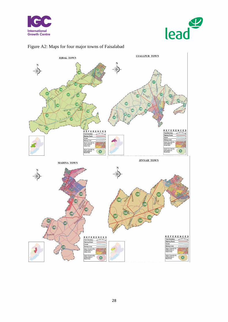
1http://www.pbs.gov.pk/sites/default/files//tables/District%20at%20a%20glance%20Faisalabad.pdf 2http://www.faisalabad.gov.pk/Home/CityProfileDetail/3 3Figure A2 in the appendix shows maps of all four towns Further details can be found on the following website:http://www.faisalabad.gov.pk/Home/Towns
6
Besides WASA, there is a range of private water supply sources in Faisalabad. These range
from unfiltered canal side pumped water to filtered bottled water. Many private sector
providers supply filtered water and non-filtered sweet groundwater pumped from canal-side
areas. Various sources of water supply in Faisalabad include, i) Canal-side pumped water ii)
Bottled water (such as, Nestle, Aquafina, Gourmet) iii) Unfiltered Sweet water iv) Small
scale filtration plantsv) Large commercial filtration plants, vi) Government filtration plants,
vii) Groundwater bore, and viii) Tankers.
The Tariff Structure
WASA water charges depend on the house size, which vary from PKR. 83 (2.5 Marla house)
per month to PKR 966 (40 Marla) per month. In addition, it charges one time water
connection fee of PKR 483, PKR 3220, and PKR 3200 for residential, commercial and
industrial usage, respectively. The current tariff plan of WASA is effective from 2006. In
Fiscal year 2010-11, WASA collected total revenues of PKR 735.03 million4. However, low
recovery rate of water bills has been a major challenge for WASA. The city government is
spending large amount of money for provision of free filtered water. Moreover, price
charged for the pipe water connection is substantially lower than the market prices, due to
high subsidies.
WASA neither charges aquifer fee for extraction of ground water for domestic use, nor does
it limit the water usage, which might have created demand supply imbalances and
inefficiencies in water market. As a result, a large proportion of households in Faisalabad
have installed domestic borings to extract groundwater. They can thus consume unlimited
water extracted from these borings,, consequently leadingto water scarcity issues.
4See details on WASA, Faisalabad website: www.wasafaisalabad.gop.pk
7
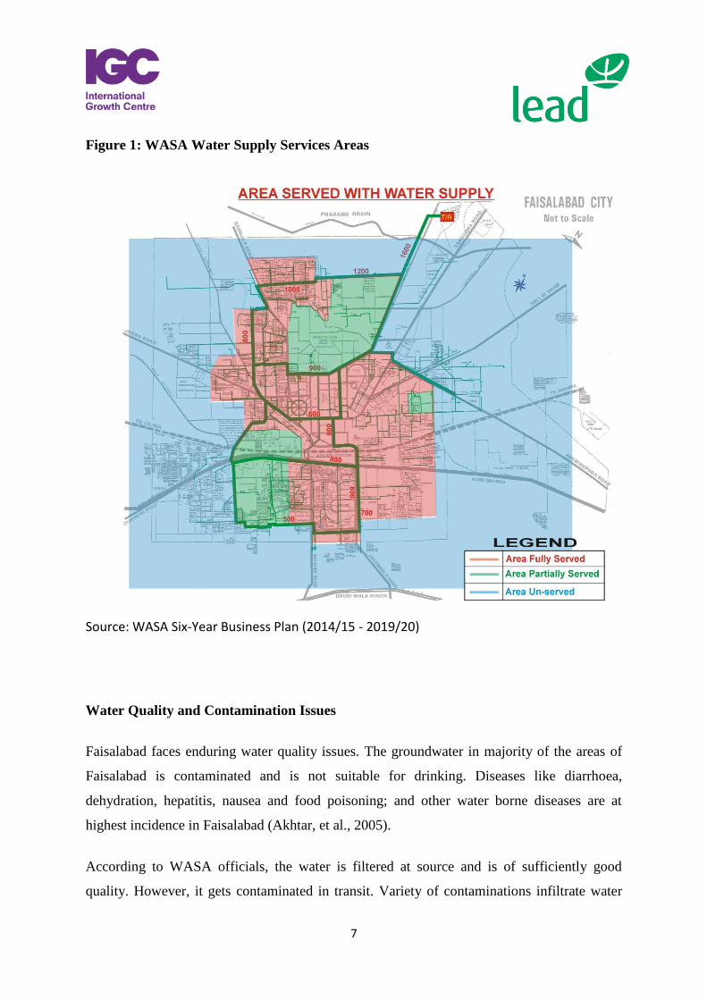
Figure 1: WASA Water Supply Services Areas
Source: WASA Six-Year Business Plan (2014/15 - 2019/20)
Water Quality and Contamination Issues
Faisalabad faces enduring water quality issues. The groundwater in majority of the areas of
Faisalabad is contaminated and is not suitable for drinking. Diseases like diarrhoea,
dehydration, hepatitis, nausea and food poisoning; and other water borne diseases are at
highest incidence in Faisalabad (Akhtar, et al., 2005).
According to WASA officials, the water is filtered at source and is of sufficiently good
quality. However, it gets contaminated in transit. Variety of contaminations infiltrate water
8
due to pipe leakages and exposure to sewerage lines. Degradedwater infrastructure and
inability of WASA to cover operations and maintenance costs have resulted in supply of
contaminated water. Piped water supplied by WASA is largely considered as unfiltered.
3. Review of Existing Literature
Water pricing has been a longstanding issue. Researchers have proposed various approaches
to analyse different tariff structures by estimating demand function and calculating respective
price and income elasticities (see for a survey, Arbues et al., 2003; Nauges and Whittington,
2010). Despite the fact that water demand analysis in developing economies started a long
time ago (White et al., 1972; Katzman, 1977), yet there exists a limited literature. The
analysis of demand for water in developing economies is complex, as different household
groups use multiple sources to meet their water demand, which needs a careful analysis to
draw appropriate inferences for policy making (Nauges and Wittington, 2010).
Though, vast literature focuses on household demand for water in developed economies, until
1970s most of the studies on residential water demand have been mainly devoted to the
United States, where some regions had been affected by periods of severe drought (Howe and
Linaweaver, 1967; Gibbs 1978; Danielson, 1979; Foster and Beattie, 1979). In the 1980s,
many studies on residential water demand focused on economic analysis using econometrics
methods (Agthe and Billings, 1980; Schefter and David, 1985; Chicoine and Ramamurthy,
1986; Nieswiadomy and Molina, 1989 among others). In the 1990s, researchers emphasized
new insights, such as adoption of low-flow equipmentby households, welfare consequences
of a price regulation, and case studies of European countries (Point, 1993; Hansen, 1996;
Agthe and Billings, 1996; Renwick and Archibald, 1998; Hoglund, 1997).In the 2000s, the
researchers considered the importance of threshold price levels (see, for details, Martínez-
Espiñeira and Nauges, 2004). In general, price elasticity remains inelastic, and estimates
vary between -0.10 and -0.30 (Hoglund, 1999; Nauges and Thomas, 2000; Martınez-
Espineira, 2002). Strand and Walker (2005) used a household survey data from 17 cities in
Central America and Venezuela, to estimate price elasticities for piped and non-piped
households, which range from −0.3 to −0.1, respectively. Using the same dataset, Nauges and
Strand (2007), determined water demand for non-piped households in four cities of El
Salvador and Honduras. Their results show that non-tap water demand elasticities range
9
between −0.4 and −0.7. Using cross-sectional household-level data from seven provincial
Cambodian towns, Basani et al. (2008) calculated the price elasticity of water demand for
connected households in the range of −0.4 and −0.5.
An empirical analysis of water demand function in developing countries is less focused,
because of unavailability of data. The water consumptions are not always metered. Therefore,
well designed surveys are required to collect the quality household level data. Particularly,
data information on the conditions of access to different water sources (price, quality,
reliability distance to the source of water, time to commute the water, and the mode to
commute the water) are important (see Mu et al. 1990, for related discussion).
McPhail (1994)addressed the question that why don’t households connect to the piped water
system, using a survey in rural areas of Tunis and Tunisia. Survey results indicate that
households cannot afford to pay for piped connections. Persson (2002) analysed the choice of
households in Philippines for drinking water sources. They argue that demand for clean water
for drinking purposes is derived demand, as it is an input to produce health. Results indicate
that time cost (price coefficient) has significant effect on choice probabilities. Results also
indicate that tastes of households have insignificant effect on choice probabilities.
Recently, Nauges and Berg(2009)have used 1,800 Sri Lankan households’ data to estimate
demand for piped and non-piped water sources. They argue that water supply service in many
developing countries is at very low level for residential consumers.They simultaneously
estimate the substitutability/complementarity between piped and non-piped water sources,
using a system equations.The results of their study show that price elasticity of demand for
piped water consumers is −0.15, whereas households relying on piped water as well as other
sources to supplement their water consumption have higher demand elasticity of −0.37. They
also find evidence of substitutability between water from different sources.
Nauges and Whittington (2009) provide a review of different econometric methods that
researchers have used to estimate water demand in developing countries and highlight issues
related to data collection in developing countries. In developing countries, most estimates of
own-price elasticity of water from private connections are in the range from -0.3 to -0.6 and
income elasticity is 0.1 to 0.3,which is close to usually reported for developed countries.
10
They further argue that empirical results related to household decision for water sources are
less robust, which need some rigorous analysis to obtain robust and reliable demand elasticity
estimates.
Wang and Li (2010) analyse willingness to pay for water, using multiple bounded discrete
choice (MBDC) survey model, with a survey of 1,500 households in five suburban districts in
Chongqing Municipality. They show that a significant increase in water price is economically
feasible, as long as the poorest households are properly subsidized. Furthermore, results show
that model has four statistically significant socioeconomic variables like household (HH)
income is an important and significant determinant of willingness to pay (WTP). But
municipal water supply system, average monthly water use and age don’t have any
significant effect on household WTP.
There are mixed findings about the demand and income elasticities of water in developing
economies, which have different important policy implications for water management bodies
in these countries. The precise and accurate estimation of price and income elasticities would
inform policy makers, how and to what extent these results can be helpful to devise viable
water-demand management policies. Particularly, it is difficult to obtain robust empirical
findings in presence of diverse water consumer groups. Therefore, it is important to estimate
separate demand functions for specific group to infer precise policy implications. This paper
analyses demand elasticities and impact of other explanatory variables on water consumption
for different groups in urban dwellings of Faisalabad city. This is the first study of such kind
in Pakistan, which suggests important policy recommendations for urban water management
authorities in Pakistan. It also provides useful insights for developing economies, in general.
4. Methodology and Data
4.1 Empirical Model
Conventionally, the demand function of a representative household is specified as a single
equation of the form:
11
Where isthe vector of N x 1 quantities; represents the vector of N x 1 prices; is a
vector of exogenous variables; and represents the vector of N x 1 random error term.
Equation (1) describes the relationship between water consumption ( ), the price (p) of
water, and a vector of household characteristics ( ) to control for heterogeneity of
preferences and other factors affecting water consumption.
Generally, the single-equation approach is used by to estimate demand for water from a
particular source, such as piped (see for instance, Crane, 1994; Rietveld et al., 2000; Basani et
al., 2008). The estimation of (single) source-specific demand equation enables us to estimate
price and income elasticities of demand.
To estimate the price and income elasticities of demand for drinking water, the linear
econometric specification is setup as
where, β and measure the effects of observable prices ( and other households
characteristics ( on . , captures unobserved effects on .
Our primary goal is to analyse the price and income elasticities of water demand, which are
represented in the following equations (3) and (4).
where represents a change in quantity demanded, is price change, and are
actual price and quantity demanded, respectively. The right hand sides of equations (3) and
(4) represent the log-log specification to estimate the respective elasticities directly.
12
We include three different demand specifications in our model. First, we estimate a combined
demand function to create baseline estimates of demand and income elasticities, along with
other exogenous factors influencing the household water demand. In the case of Faisalabad,
quality of water is a significant factor affecting consumer preferences and water usage. The
households use various types of water, which can be grouped into low and high quality of
water. Therefore, we also estimate a subsample of demand for filtered and unfiltered water,
represented by equation (5).
where, represents the quantities of water consumed by individual household from
different sources (such that ; ,
represents the vector of household characteristics and other factors affecting the water
demand, which include income, age, education, distance from water facility, and tank water;
and represents dummy variables for piped connection, house storeys, and filtered water
consumption, respectively.
The regulated pricing mechanism, adopted by water providers in many countries may cause
endogeneity problems, which in turn will produce biased and inconsistent estimates. This
may be the case with WASA, where price-setting mechanism could influence water prices.
Several studies have used instrumental variable methods to address the endogeneity issues in
water demand estimation (E.g., Schleich and Hillenbrand, 2009; Nauges and Berg, 2009).
These studies either use two-stage least square (2SLS) or generalized methods of moments
(GMM) for estimating simultaneous equations or single structural models (See, for example,
Chicoine et al., 1986; Stevens et al., 1992; Strand and Walker, 2005; Nauges and Strand,
2007; Naugas and Berg, 2009; Schleich and Hillenbrand, 2009). To address the problem of
endogeneity using instrumental variable techniques, such as two-stage least squares (2SLS)
regression, where the water price is explained by instruments uncorrelated with the error term
of the water demand equation. In order to control potential problem of endogeneity, we use
single equation ordinary least square (OLS) and instrumental variables (IV) approach.We use
single OLS and IV estimation procedures to evaluate price and income elasticities of demand
13
for German residents. For instance, Limited Information Maximum Likelihood (LIML)
computes the limited information maximum likelihood estimator for a single equation linear
structural model. LIML determines the list of endogenous variables, included exogenous
variables, and excluded exogenous variables by comparing the instrument list with the
variables in the equation.
4.2 Sample Selection and Data Description
District Faisalabad has a total population of 5,429,547 according to the 1998 census, with an
urban population of 2,318,433 (42.70 %) and a rural population of 3,111,114 (52.30 %)
(Pakistan Bureau of Statistics)5. In 2005, District Faisalabad is divided into eight towns,with
a Town Municipal Administration (TMA) for each town (City District Government
Faisalabad)6. However, within these the urban areas (or in other words Faisalabad city) is
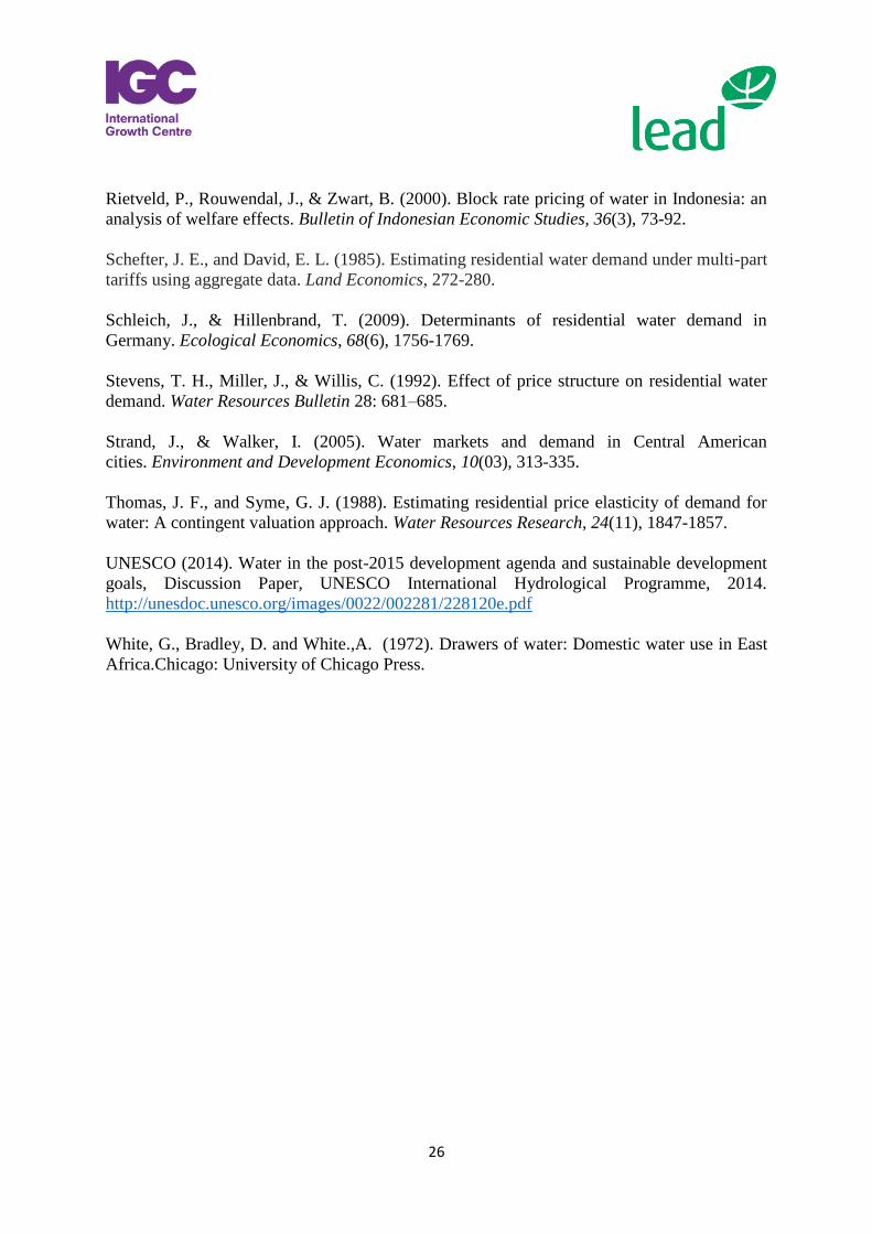
comprised of four towns and cover about 88 percent of urban population living in these
towns.These include, Iqbal Town, Jinnah Town, Lyallpur Town and Madina Town (see Table
A1 in the appendix). Whereas the remaining four towns cover the rural population. Hence,
we chose these four towns to cover out target population i.e. Faisalabad city. These four town
also include sub-urban areas and kachi abadis so we are not excluding them.We used
stratified sampling technique to collect household data and focused on fourmain towns.Their
respective population is presented in Table A1 in the appendix.
Data Description
Sources of Drinking Water
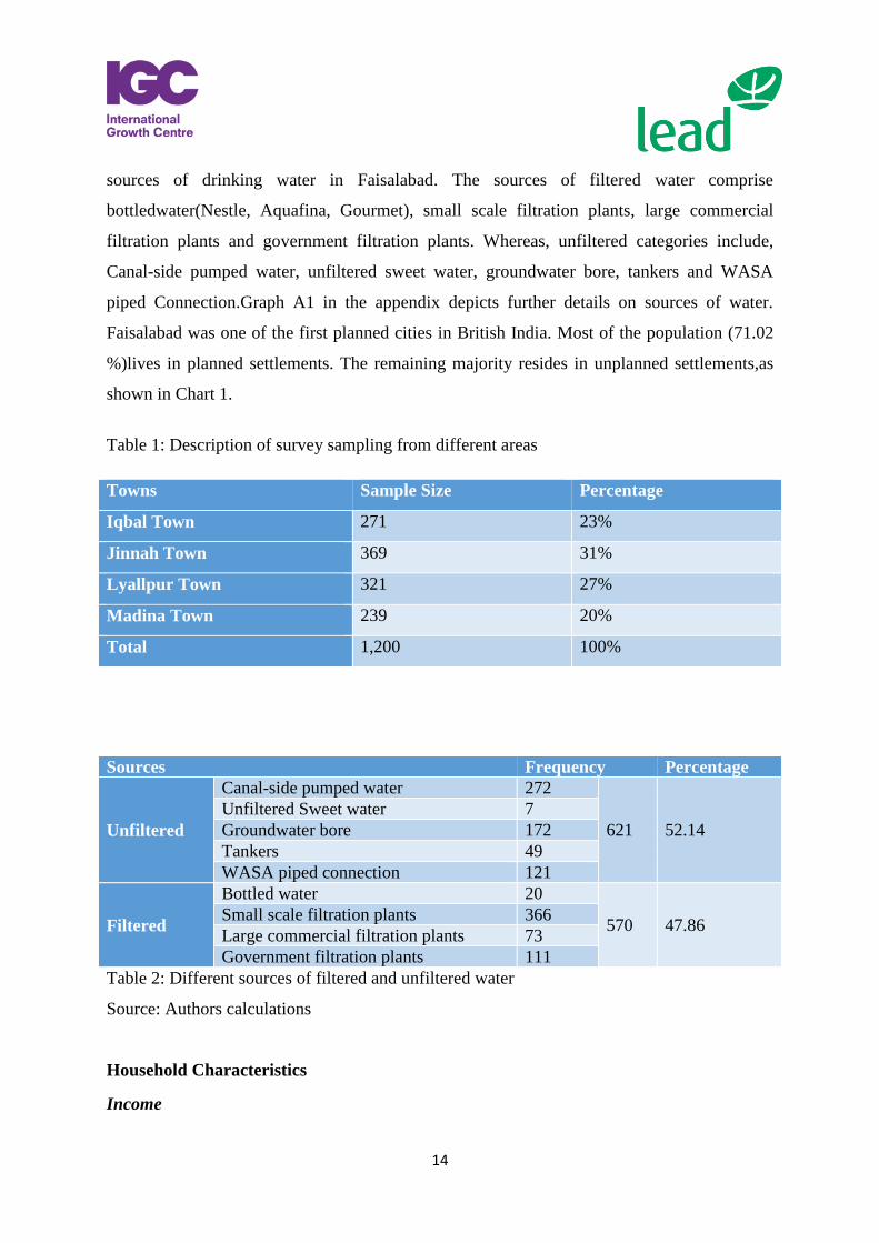
The study draws proportional sampling from all four towns.Sample size is described in Table
1. The collected sample represents water consumption from multiple sources, including
filtered and unfiltered water and private and government supplies. Table 2 presents the
various sources of water used by the sample households. The sample comprises 570
households (HH) (47.86%) consuming filtered water, and 621 HH (52.14%) consuming
unfiltered water. Filtered and unfiltered water are further subdivided into nine primary
5http://www.pbs.gov.pk/sites/default/files//tables/District%20at%20a%20glance%20Faisalabad.pdf 6http://www.faisalabad.gov.pk/Home/Towns
14
sources of drinking water in Faisalabad. The sources of filtered water comprise
bottledwater(Nestle, Aquafina, Gourmet), small scale filtration plants, large commercial
filtration plants and government filtration plants. Whereas, unfiltered categories include,
Canal-side pumped water, unfiltered sweet water, groundwater bore, tankers and WASA
piped Connection.Graph A1 in the appendix depicts further details on sources of water.
Faisalabad was one of the first planned cities in British India. Most of the population (71.02
%)lives in planned settlements. The remaining majority resides in unplanned settlements,as
shown in Chart 1.
Table 1: Description of survey sampling from different areas
Table 2: Different sources of filtered and unfiltered water
Source: Authors calculations
Household Characteristics
Income
Towns Sample Size Percentage
Iqbal Town 271 23%
Jinnah Town 369 31%
Lyallpur Town 321 27%
Madina Town 239 20%
Total 1,200 100%
Sources Frequency Percentage
Unfiltered
Canal-side pumped water 272
621 52.14
Unfiltered Sweet water 7
Groundwater bore 172
Tankers 49
WASA piped connection 121
Filtered
Bottled water 20
570 47.86 Small scale filtration plants 366
Large commercial filtration plants 73
Government filtration plants 111
15
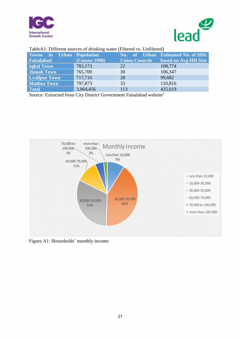
The sample data depicts that the average household income is PKR. 33,966. Sample statistics
show that about 51 percent of the respondents belong to lower or middle income group(See
Graph A2 in the appendix). For instance, nine percent of the households have less than PKR.
10,000 monthly income, whereas 42 percent earn between PKR. 10,000-30,000 per month,
which is followed by income group of PKR. 30,000-50000, that comprises 31 percent of the
entire sample. About 11 % of the sample represents households having monthly income
between PKR. 50,000-70,000. Whereas, the income group earning PKR.70,000-100,000
makes five percent of the sample. Two percent of the sample represents high income group
above PKR. 100,000).
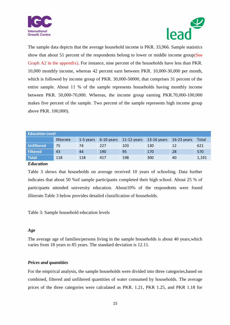
Education
Table 3 shows that households on average received 10 years of schooling. Data further
indicates that about 50 %of sample participants completed their high school. About 25 % of
participants attended university education. About10% of the respondents were found
illiterate.Table 3 below provides detailed classification of households.
Table 3: Sample household education levels
Age
The average age of families/persons living in the sample households is about 40 years,which
varies from 18 years to 85 years. The standard deviation is 12.11.
Prices and quantities
For the empirical analysis, the sample households were divided into three categories,based on
combined, filtered and unfiltered quantities of water consumed by households. The average
prices of the three categories were calculated as PKR. 1.21, PKR 1.25, and PKR 1.18 for
Education Level
Illiterate 1-5 years 6-10 years 11-12 years 13-16 years 16-23 years Total
Unfiltered 75 74 227 103 130 12 621
Filtered 43 44 190 95 170 28 570
Total 118 118 417 198 300 40 1,191
16
combined, filtered and unfiltered waterconsumed per litre, respectively. Similarly, average
respective quantities for the above said three categories were recorded on average 273 litres,
124 litres and 285 litres weekly.
3. Results and Discussion
This section discusses empirical results on household demand for water and other factors
affecting the willingness to pay. Table A3-A5 in the appendix present the correlations
coefficients of variables used in the demand estimation for combined, filtered and unfiltered
data groups. Asingle equation demand model was separately estimated each type of water
(filtered, unfiltered). The following steps were adopted in empirical analysis. Firstly, demand
function was estimated for combined sample of filtered and unfiltered water to calculate price
and income elasticities of demand using OLS. Secondly, separate residential water demand
functions were estimated for sub-samples of filtered and unfiltered water. Lastly,
instrumental variables approach was usedin to address likely issues of endogeneity.
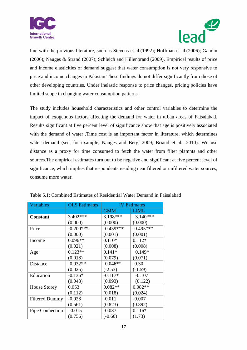
Table 5.1 reports results of OLS and IV estimates of residential water demand for a combined
sample of filtered and unfiltered water. OLS estimates presented in column two and their
respective p-values in parenthesis show that own price elasticity of demand is negative and
significant at one percent level of significance. All estimates are based on log-log model to
directly infer the price and income elasticities of water demand. The coefficient of own price
elasticity (0.20) suggests that demand is inelastic, implying that 1 % increase in the price of
water causes 0.20% decline in the quantity demand of water.These results are comparable
with the earlier studiesreported in the existing literature (see for instance, Agthe and Billings,
1980; Chicoine et al.,1986; Thomas and Syme, 1988; Renwick et al., 1998; Nauges and
Thomas, 2000; Gaudin et al., 2001; and Dharmaratna, Harris, 2012).The low magnitude
elasticity indicates that household have relatively low share of water spending in their total
expenditures.
Estimate of income remains significantly positive (i.e., 0.096), implying that households with
higher income consume more water. In terms of income elasticity of demand, one percent
increase in income leads to 0.18% increase in demand of water. The income elasticities are in
17
line with the previous literature, such as Stevens et al.(1992); Hoffman et al.(2006); Gaudin
(2006); Nauges & Strand (2007); Schleich and Hillenbrand (2009). Empirical results of price
and income elasticities of demand suggest that water consumption is not very responsive to
price and income changes in Pakistan.These findings do not differ significantly from those of
other developing countries. Under inelastic response to price changes, pricing policies have
limited scope in changing water consumption patterns.
The study includes household characteristics and other control variables to determine the
impact of exogenous factors affecting the demand for water in urban areas of Faisalabad.
Results significant at five percent level of significance show that age is positively associated
with the demand of water .Time cost is an important factor in literature, which determines
water demand (see, for example, Nauges and Berg, 2009; Briand et al., 2010). We use
distance as a proxy for time consumed to fetch the water from filter plamnts and other
sources.The empirical estimates turn out to be negative and significant at five percent level of
significance, which implies that respondents residing near filtered or unfiltered water sources,
consume more water.
Table 5.1: Combined Estimates of Residential Water Demand in Faisalabad
Variables OLS Estimates IV Estimates
GMM LIML
Constant 3.402***
(0.000)
3.198***
(0.000)
3.140***
(0.000)
Price -0.200***
(0.000)
-0.459***
(0.001)
-0.495***
(0.001)
Income 0.096**
(0.021)
0.110*
(0.008)
0.112*
(0.008)
Age 0.123**
(0.018)
0.141*
(0.079)
0.149*
(0.071)
Distance -0.032**
(0.025)
-0.046**
(-2.53)
-0.30
(-1.59)
Education -0.136*
(0.043)
-0.117*
(0.093)
-0.107
(0.122)
House Storey 0.053
(0.112)
0.082**
(0.018)
0.082**
(0.024)
Filtered Dummy -0.028
(0.561)
-0.011
(0.823)
-0.007
(0.892)
Pipe Connection 0.015
(0.756)
-0.037
(-0.60)
0.116*
(1.73)
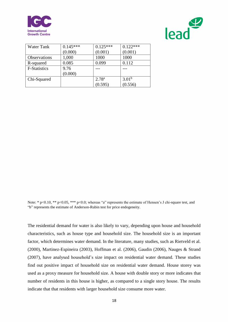
18
Note: * p<0.10, ** p<0.05, *** p<0.0; whereas “a” represents the estimate of Hensen’s J chi-square test, and
“b” represents the estimate of Anderson-Rubin test for price endogeneity.
The residential demand for water is also likely to vary, depending upon house and household
characteristics, such as house type and household size. The household size is an important
factor, which determines water demand. In the literature, many studies, such as Rietveld et al.
(2000), Martinez-Espineira (2003), Hoffman et al. (2006), Gaudin (2006), Nauges & Strand
(2007), have analysed household’s size impact on residential water demand. These studies
find out positive impact of household size on residential water demand. House storey was
used as a proxy measure for household size. A house with double story or more indicates that
number of residents in this house is higher, as compared to a single story house. The results
indicate that that residents with larger household size consume more water.
Water Tank 0.145***
(0.000)
0.125***
(0.001)
0.122***
(0.001)
Observations 1,000 1000 1000
R-squared 0.085 0.099 0.112
F-Statistics 9.76
(0.000)
--- ---
Chi-Squared 2.78a
(0.595)
3.01b
(0.556)
19
Other dummy variables were introduced in empirical model to assess whether the use of
different water sources significantly drives the household water consumption or not. To this
end, a dummy variable was introduced for households using filtered water (filtered =1, 0
otherwise). The households using filtered water consume less water, as compared to those
using unfiltered water. However, this impact is insignificant. In addition, dummy variable
was used for piped connection. Its results show positive relationship with water consumption.
In other words, households with WASA connection are likely to use more water, compared
with those, which do not have piped water facility. Similarly, results estimates of households
using tank water remain significantly positive, meaning that one percent increase in tank
water use, increases overall water consumption by 0.15 percent.
Considering the water price-setting mechanism by WASA in Faisalabad, prices may have
been treated endogenously, and thus violate the orthogonality conditions, as price is
correlated with the random terror term. Instrumental methods were used to control the
endogeneity issues, while estimating the demand elasticities. Limited information maximum
likelihood function (LIML) and Generalized moment method (GMM) were applied to
estimate the single demand equation, while using valid instruments in each specification.
Hansen chi-square, and Basmann tests were applied to check the validity of instruments (See
Table 1). The p-values of these tests indicate that the null hypothesis of exogeneity of the
instruments cannot be rejected. In other words, the instruments used in the estimation
procedures are valid. Our estimates results from OLS and instrumental variable methods are
similar, except the price elasticities estimates.However, these differences in magnitudes do
not impact pricing policy implications.
Table 5.1 reports results for price and income elasticity of demand, based on instrumental
variable method estimation. Price was instrumented with geographical indicator distance,
media as an awareness indicator, and pipe leakages as water quality indicator.The price
elasticity of demand is found -0.46 and -0.50 for GMM and LIML estimation, respectively.
The magnitude of own price elasticity of demand has increased after using IV method. It is
consistent with other studies, such as Martin and Thomas (1986), Dandy et al. (1997),
Hoffman et al. (2006), Martinez-Espineira (2007), Nauges & Whittington (2009), de Maria
20
Andre and Carvalho (2014).Though the price elasticities estimates from IV methods are
double in magnitude, yet these remain inelastic.
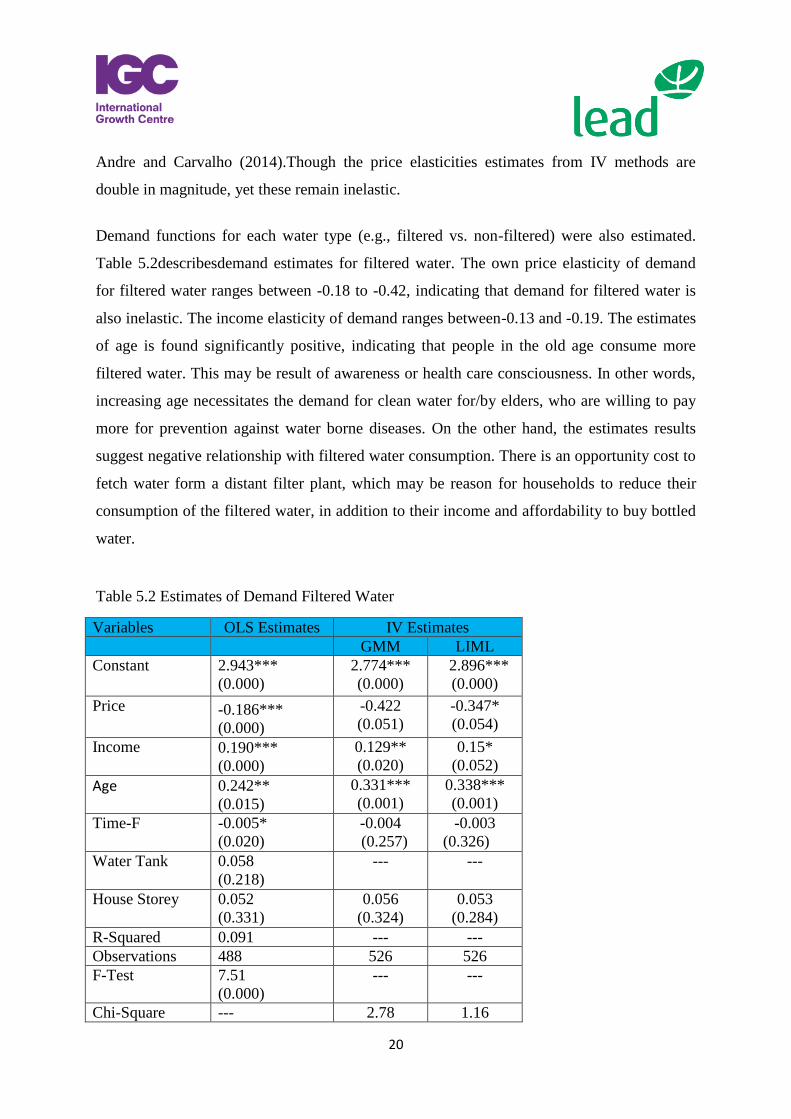
Demand functions for each water type (e.g., filtered vs. non-filtered) were also estimated.
Table 5.2describesdemand estimates for filtered water. The own price elasticity of demand
for filtered water ranges between -0.18 to -0.42, indicating that demand for filtered water is
also inelastic. The income elasticity of demand ranges between-0.13 and -0.19. The estimates
of age is found significantly positive, indicating that people in the old age consume more
filtered water. This may be result of awareness or health care consciousness. In other words,
increasing age necessitates the demand for clean water for/by elders, who are willing to pay
more for prevention against water borne diseases. On the other hand, the estimates results
suggest negative relationship with filtered water consumption. There is an opportunity cost to
fetch water form a distant filter plant, which may be reason for households to reduce their
consumption of the filtered water, in addition to their income and affordability to buy bottled
water.
Table 5.2 Estimates of Demand Filtered Water
Variables OLS Estimates IV Estimates
GMM LIML
Constant 2.943***
(0.000)
2.774***
(0.000)
2.896***
(0.000)
Price -0.186***
(0.000)
-0.422
(0.051)
-0.347*
(0.054)
Income 0.190***
(0.000)
0.129**
(0.020)
0.15*
(0.052)
Age 0.242**
(0.015)
0.331***
(0.001)
0.338***
(0.001)
Time-F -0.005*
(0.020)
-0.004
(0.257)
-0.003
(0.326)
Water Tank 0.058
(0.218)
--- ---
House Storey 0.052
(0.331)
0.056
(0.324)
0.053
(0.284)
R-Squared 0.091 --- ---
Observations 488 526 526
F-Test 7.51
(0.000)
--- ---
Chi-Square --- 2.78 1.16
21
(0.595) (0.312) Note: * p<0.10, ** p<0.05, *** p<0.01;
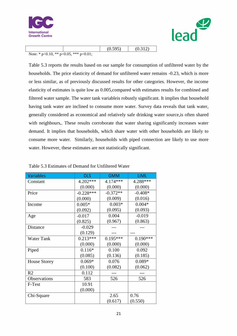
Table 5.3 reports the results based on our sample for consumption of unfiltered water by the
households. The price elasticity of demand for unfiltered water remains -0.23, which is more
or less similar, as of previously discussed results for other categories. However, the income
elasticity of estimates is quite low as 0.005,compared with estimates results for combined and
filtered water sample. The water tank variableis robustly significant. It implies that household
having tank water are inclined to consume more water. Survey data reveals that tank water,
generally considered as economical and relatively safe drinking water source,is often shared
with neighbours,. These results corroborate that water sharing significantly increases water
demand. It implies that households, which share water with other households are likely to
consume more water. Similarly, households with piped connection are likely to use more
water. However, these estimates are not statistically significant.
Table 5.3 Estimates of Demand for Unfiltered Water
Variables OLS GMM LIML Constant 4.202***
(0.000)
4.174***
(0.000)
4.288***
(0.000)
Price -0.228***
(0.000)
-0.372**
(0.009)
-0.408*
(0.016)
Income 0.005*
(0.092)
0.003*
(0.095)
0.004*
(0.093)
Age -0.017
(0.825)
0.004
(0.967)
-0.019
(0.863)
Distance -0.029
(0.129)
---
---
---
---
Water Tank 0.213***
(0.000)
0.195***
(0.000)
0.190***
(0.000)
Piped 0.116*
(0.085)
0.100
(0.136)
0.092
(0.185)
House Storey 0.069*
(0.100)
0.076
(0.082)
0.089*
(0.062)
R2 0.112 --- ---
Observations 583 526 526
F-Test 10.91
(0.000)
Chi-Square 2.65
(0.617)
0.76
(0.550)
22
Note: * p<0.10, ** p<0.05, *** p<0.01
4. Conclusion
This study examined urban residential water use in Faisalabad, to identify the factors which
influence variability of household water demand. Econometric methods were used to estimate
the price and income elasticities of water demand across different groups of consumers.
Study used a survey data of 1,200 households, collected from urban residents of Faisalabad–
one of the largest city and industrial hub of Pakistan. Researchers applied OLS and IV
methods to address endogeneity issues, which otherwise could produce biased and
inconsistent estimates, due to price setting. However, results do not provide any evidence of
price endogeneity. Generally, empirical results of OLS and IV methods are similar, except
some differences in magnitude of price and income elasticities. The price elasticity estimates
of IV procedure were double than OLS estimates. Never the less, the demand remains price
inelastic, across all consumer groups. Specifically, estimates of price for combined sample
varied from -0.20 to -0.45, while estimates for filtered and unfiltered water ranged from -0.19
to -0.42 and -0.23 to -0.41, respectively. These findings are similar to many developed and
developing countries’ estimates, suggesting that water demand in Faisalabad is likely to
respond less to increase in prices. In other words, pricing policies may have limited scope in
changing water consumption.
Findings reflect that income elasticities vary significantly across different groups (i.e., from
0.005 to 0.19). It is noticeable that income elasticity significantly decreases, in case of filtered
water consumers’ group. In other words, water consumption changes disproportionately, with
varying income levels. This divergence in water consumption seems to be due to differences
in income levels and social status.
Other possible factors to analyse the water consumption differences across groups, include
age, distance to water facility, education and water connections. Results show that age is
positively and significantly associated with the demand of filtered water. Furthermore, in the
case of unfiltered water, the results show that water sharing significantly increases water
23
demand. The impact of distance to water source is negative implying, that households
residing near water sources tend to consume more water. The policy implication of this
finding could be focus on locational and supply side factors of water. The government
intervention to increase water supply points or direct supply of clean water can substantially
affect the residential water demand.
The findings of the study also suggest that non-pricing tools, such as creating water saving
awareness through educational campaigns, informational tools and encouraging use of water
efficient devices can be helpful in saving water. Pricing signals that come from health
awareness about the benefits of clean water, must remain an essential part of public
management in Pakistan. The household demand estimates inform various key messages for
water planning management of Faisalabad, WASA. These messages include the need for
appropriate pricing structure, and improving the water supply infrastructure in the urban
areas.
Lastly, to achieve the goals of clean and sustainable water consumption, the local government
and Water and Sanitation Authorities need to increase the coverage of drinking water
facilities in priority low income areas, that lag behind other dwellings. This calls for the need
of appropriate policies, for ensuring equity by removing disparities.
24
5. References
Agthe, D. E., and Billings, R. B. (1980). Dynamic models of residential water demand. Water
Resources Research, 16(3), 476-480.
Agthe, D. E., and Billings, R. B. (1996). Water-price effect on residential and apartment low-
flow fixtures. Journal of water resources planning and management, 122(1), 20-23.
Akhtar, N., Jamil, A., Noureen, H., Imran, M., Iqbal, I., and Alam, A. (2005). Impact of
Water Pollution on Human Health in Faisalabad City. Pakistan Journal of Agriculture &
Social Sciences, 1(1): 43–44.
Arubes, F., Gracia-Valinas, M. A. and Martinez-Espeneira, R. (2003). Estimation of
residential water demand: A state of the art review. Journal of Socioeconomic, 32, 81-102.
Briand, A., Nauges, C., Strand, J., and Travers, M. (2010). The impact of tap connection on
water use: the case of household water consumption in Dakar, Senegal. Environment and
Development Economics, 15(01), 107-126.
Chicoine, D. L., & Ramamurthy, G. (1986). Evidence on the specification of price in the
study of domestic water demand. Land Economics, 26-32.
Crane R (1994). Water markets, market reform and the urban poor: results from Jakarta,
Dandy, G., Nguyen, T., & Davies, C. (1997). Estimating residential water demand in the
presence of free allowances. Land Economics, 125-139.
de Maria André, D., & Carvalho, J. R. (2014). Spatial determinants of urban residential water
demand in Fortaleza, Brazil. Water Resources Management, 28(9), 2401-2414.
Dharmaratna, D., & Harris, E. (2012). Estimating residential water demand using the stone-
geary functional form: the case of Sri Lanka. Water Resources Management, 26(8), 2283-
2299.
Foster, H. S., and Beattie, B. R. (1979). Urban residential demand for water in the United
States. Land Economics, 43-58.
Gaudin, S. (2006). Effect of price information on residential water demand. Applied
Economics, 38(4), 383-393.
Gaudin, S., Griffin, R. C., & Sickles, R. C. (2001). Demand specification for municipal water
management: evaluation of the Stone-Geary form. Land Economics, 77(3), 399-422.
Hoffmann, M., Worthington, A., & Higgs, H. (2006). Urban water demand with fixed
volumetric charging in a large municipality: the case of Brisbane, Australia*. Australian
Journal of Agricultural and Resource Economics, 50(3), 347-359.
25
Howe, C. W., & Linaweaver, F. P. (1967). The impact of price on residential water demand
and its relation to system design and price structure. Water Resources Research, 3(1), 13-
http://www.peacebuilding.no/var/ezflow_site/storage/original/application/4c5b5fa0ebc5684d
a2b9f244090593bc.pdf
Indonesia. World Dev 22(1):71–83. doi:10.1016/0305-750X(94)90169-4
Katzman, M. (1977). Income and price elasticities of demand for water in developing
countries.Water Resources Bulletin, 13:47–55.
Kenway, J. S. & Lant, P. A. (2015). How does energy efficiency effect urban water system?
In Grafton Q., Daniell, K., Nauges, C., Rinaudo J. & Chan, N W, editors. Understanding ad
Managing Water in Transition (Eds.), Springer.
Kugelman, M. (2013). Urbanization in Pakistan: Causes and consequences, Norwegian
Peacebuilding Resource Centre.
Martin, W. E., & Thomas, J. F. (1986). Policy relevance in studies of urban residential water
demand. Water Resources Research, 22(13), 1735-1741.
Martínez-Espiñeira, R. (2002). Residential water demand in the Northwest of
Spain. Environmental and resource economics, 21(2), 161-187.
Martinez-Espineira, R. (2003). Estimating water demand under increasing-block tariffs using
aggregate data and proportions of users per block. Environmental and resource
economics, 26(1), 5-23.
Martínez-Espineira, R. (2007). An estimation of residential water demand using co-
integration and error correction techniques. Journal of Applied Economics, 10(1).
Nauges, C., & Strand, J. (2007). Estimation of non-tap water demand in Central American
cities. Resource and Energy Economics, 29(3), 165-182.
Nauges, C., & Thomas, A. (2000). Privately operated water utilities, municipal price
negotiation, and estimation of residential water demand: the case of France. Land Economics,
68-85.
Nauges, C., & Van Den Berg, C. (2009). Demand for piped and non-piped water supply
services: Evidence from Southwest Sri Lanka. Environmental and Resource
Economics, 42(4), 535-549.
Nauges, C., & Whittington, D. (2010). Estimation of water demand in developing countries:
An overview. The World Bank Research Observer, 25(2), 263-294.
Nieswiadomy, M. L., & Molina, D. J. (1989). Comparing residential water demand estimates
under decreasing and increasing block rates using household data. Land Economics, 280-289.
Renwick, M. E., & Archibald, S. O. (1998). Demand side management policies for residential
water use: who bears the conservation burden? Land economics, 343-359
26
Rietveld, P., Rouwendal, J., & Zwart, B. (2000). Block rate pricing of water in Indonesia: an
analysis of welfare effects. Bulletin of Indonesian Economic Studies, 36(3), 73-92.
Schefter, J. E., and David, E. L. (1985). Estimating residential water demand under multi-part
tariffs using aggregate data. Land Economics, 272-280.
Schleich, J., & Hillenbrand, T. (2009). Determinants of residential water demand in
Germany. Ecological Economics, 68(6), 1756-1769.
Stevens, T. H., Miller, J., & Willis, C. (1992). Effect of price structure on residential water
demand. Water Resources Bulletin 28: 681–685.
Strand, J., & Walker, I. (2005). Water markets and demand in Central American
cities. Environment and Development Economics, 10(03), 313-335.
Thomas, J. F., and Syme, G. J. (1988). Estimating residential price elasticity of demand for
water: A contingent valuation approach. Water Resources Research, 24(11), 1847-1857.
UNESCO (2014). Water in the post-2015 development agenda and sustainable development
goals, Discussion Paper, UNESCO International Hydrological Programme, 2014.
http://unesdoc.unesco.org/images/0022/002281/228120e.pdf
White, G., Bradley, D. and White.,A. (1972). Drawers of water: Domestic water use in East
Africa.Chicago: University of Chicago Press.
27
TableA1: Different sources of drinking water (Filtered vs. Unfiltered)
Towns in Urban
Faisalabad
Population
(Census 1998)
No. of Urban
Union Councils
Estimated No. of HHs
based on Avg HH Size
Iqbal Town 783,173 22 108,774
Jinnah Town 765,700 30 106,347
Lyallpur Town 717,710 28 99,682
Madina Town 797,873 33 110,816
Total 3,064,456 113 425,619
Source: Extracted from City District Government Faisalabad websitei
Figure A1: Households’ monthly income
Less than 10,0009%
10,000-30,00042%
30,000-50,00031%
50,000-70,000 11%
70,000 to 100,000
5%
more than 100,000
2%
Monthly Income
Less than 10,000
10,000-30,000
30,000-50,000
50,000-70,000
70,000 to 100,000
more than 100,000
28
Figure A2: Maps for four major towns of Faisalabad
29
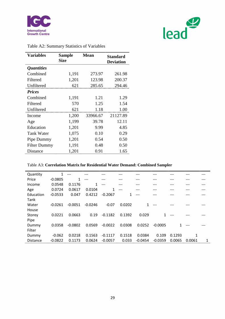
Table A2: Summary Statistics of Variables
Variables Sample
Size
Mean Standard
Deviation
Quantities
Combined 1,191 273.97 261.98
Filtered 1,201 123.98 200.37
Unfiltered 621 285.65 294.46
Prices
Combined 1,191 1.21 1.29
Filtered 570 1.25 1.54
Unfiltered 621 1.18 1.00
Income 1,200 33966.67 21127.89
Age 1,199 39.78 12.11
Education 1,201 9.99 4.85
Tank Water 1,075 0.10 0.29
Pipe Dummy 1,201 0.54 0.50
Filter Dummy 1,191 0.48 0.50
Distance 1,201 0.91 1.65
Table A3: Correlation Matrix for Residential Water Demand: Combined Sampler
Quantity 1 --- --- --- --- --- --- --- --- --- Price -0.0805 1 --- --- --- --- --- --- --- --- Income 0.0548 0.1176 1 --- --- --- --- --- --- --- Age 0.0724 0.0617 0.0104 1 --- --- --- --- --- --- Education -0.0533 0.047 0.4212 -0.2067 1 --- --- --- --- --- Tank Water -0.0261 -0.0051 -0.0246 -0.07 0.0202 1 --- --- --- --- House Storey 0.0221 0.0663 0.19 -0.1182 0.1392 0.029 1 --- --- --- Pipe Dummy 0.0358 -0.0802 0.0569 -0.0022 0.0308 0.0252 -0.0005 1 --- --- Filter Dummy -0.062 0.0218 0.1563 -0.1117 0.1518 0.0384 0.109 0.1293 1 Distance -0.0822 0.1173 0.0624 -0.0057 0.033 -0.0454 -0.0359 0.0065 0.0061 1
30
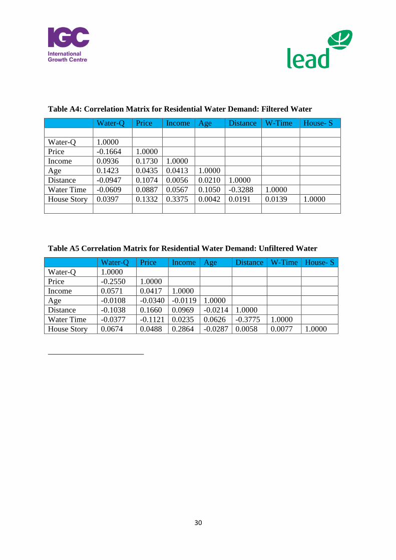
Table A4: Correlation Matrix for Residential Water Demand: Filtered Water
Water-Q Price Income Age Distance W-Time House- S
Water-Q 1.0000
Price -0.1664 1.0000
Income 0.0936 0.1730 1.0000
Age 0.1423 0.0435 0.0413 1.0000
Distance -0.0947 0.1074 0.0056 0.0210 1.0000
Water Time -0.0609 0.0887 0.0567 0.1050 -0.3288 1.0000
House Story 0.0397 0.1332 0.3375 0.0042 0.0191 0.0139 1.0000
Table A5 Correlation Matrix for Residential Water Demand: Unfiltered Water
Water-Q Price Income Age Distance W-Time House- S
Water-Q 1.0000
Price -0.2550 1.0000
Income 0.0571 0.0417 1.0000
Age -0.0108 -0.0340 -0.0119 1.0000
Distance -0.1038 0.1660 0.0969 -0.0214 1.0000
Water Time -0.0377 -0.1121 0.0235 0.0626 -0.3775 1.0000
House Story 0.0674 0.0488 0.2864 -0.0287 0.0058 0.0077 1.0000
Designed by soapbox.co.uk
The International Growth Centre (IGC) aims to promote sustainable growth in developing countries by providing demand-led policy advice based on frontier research.
Find out more about our work on our website www.theigc.org
For media or communications enquiries, please contact [email protected]
Subscribe to our newsletter and topic updates www.theigc.org/newsletter
Follow us on Twitter @the_igc
Contact us International Growth Centre, London School of Economic and Political Science, Houghton Street, London WC2A 2AE