Analysing Convergence in Europe Using a Non-linear Single

Department Economics and Politics

Analysing Convergence in Europe

Using a Non-linear Single Factor Model

Ulrich Fritsche and Vladimir Kuzin

DEP Discussion Papers

Macroeconomics and Finance Series

2/2008

Hamburg, 2008

Analysing Convergence in Europe Using a

Non-linear Single Factor Model§

Ulrich Fritsche∗ Vladimir Kuzin∗∗

June 7, 2008

Abstract

We investigate convergence in European price level, unit labor cost,income, and productivity data over the period of 1960-2006 using thenon-linear time-varying coefficients factor model proposed by Phillipsand Sul (2007). This approach is extremely flexible on order to modela large number of transition paths to convergence. We find regionalclusters in consumer price level data. GDP deflator data and unit la-bor cost data are far less clustered than CPI data. Income per capitadata indicate the existence of three convergence clubs without strongregional linkages; Italy and Germany are not converging to any of thoseclubs. Total factor productivity data indicate the existence of a smallclub including fast-growing countries and a club consisting of all othercountries.

Keywords: Price level, Income, Productivity, Convergence, FactorModel, European Monetary UnionJEL classification: E31, O47, C32, C33

§The positions do not necessarily reflect those of other persons in the institutions theauthors might be affiliated with. Thanks to Silke Bumann, Georg Erber, Michael Funke,Torsten Schunemann, Thomas Straubhaar, Andreas Strasser and Sebastian Weber forhelpful comments. All remaining errors are ours.

∗University Hamburg, Faculty Economics and Social Sciences, Department Economicsand Politics, Von-Melle-Park 9, D-20146 Hamburg, and German Institute for EconomicResearch (DIW Berlin), Germany, [email protected]

∗∗German Institute for Economic Research (DIW), Macro Analysis and Forecasting,Mohrenstraße 58, D-10117 Berlin, Germany, [email protected]

I

mailto:[email protected]

mailto:[email protected]

Convergence in Europe in a Non-linear Factor Model1 Introduction

1 Introduction

The paper investigates the process of convergence in price indices, income,and total factor productivity in a number of European countries – most ofthese countries share a common currency now.1 In the course of the paper,we apply a new and – as the authors convincingly argue – appropriate time-varying econometric framework (Phillips and Sul, 2007) which allows fortotal or subgroup convergence under a variety of possible transition paths.

The last four decades saw several waves in the process of European in-tegration: in 1968, a tariff union was established, followed by the exchangerate regime nicely labeled as a “snake in the tunnel” in 1972, the forerun-ner of the European monetary system. The European internal market wasinitiated in the 1980s and almost completed in 1992. The most remark-able part of integration process however lies in the process of monetaryintegration, culminating in the creation of a single currency and the eurocash changeover in 2002. Since then, numerous countries in the Middle andEast as well as in the South of Europe have joined the club. As BarryEichengreen argues, there is no comparable predecessor in history, thereforehistorical analogies to study the effects of European integration have theirlimits (Eichengreen, 2008). In general, the European integration processand especially the introduction of a common currency has long been seenas an huge step forward in the convergence of income and living conditions(Emerson, Gros, and Italianer, 1992). Several arguments why a commonmonetary regime should foster integration and convergence across countriesin Europe have been raised. The most prominent refers to individual priceand price level convergence: falling trade barriers as well as increased arbi-trage possibilities should speed up convergence in individual prices – at leastfor tradable goods. This process should be reinforced by a stepwise harmo-nization of financial and product market regulations (Cuaresma, Egert, andSilgoner, 2007): firms from outside the EMU will set prices for the overallunion (Devereux, Engel, and Tille, 2003). Even if the exact size of the effectis disputed (Rose and Engel, 2002), it is clear that increasing trade (Rose,2000) should spur individual price convergence further. Diminishing differ-entials in relative prices do not necessarily imply price level convergence asthe demand elasticities might differ. As Cecchetti, Mark, and Sonora (2002)show for the U.S., price level convergence is slow across cities due to a largeshare of non-traded goods (and possibly different weights in consumptionbaskets across cities). Over the long-run, differences in consumption basketsshould however diminish (Corsetti, 2008).2

1We apply the tests on a panel of EU 15 countries, keeping three countries which arenot members of the currency union in the sample as a control group exercise.

2Due to a lack of available data, we are not able to investigate this issue more deeplyhere.

1

Convergence in Europe in a Non-linear Factor Model1 Introduction

Beyond the much-disputed argument of enforced price level convergence,however, the level of other macroeconomic variables stressed in growth mod-els – e.g. per-capita income or total factor productivity – may be altered byforming a currency union. Alesina and Barro (2002) and Tenreyro and Barro(2007) argue that entering a common currency area enhances trade (Rose,2000), increases price co-movement across the member states but decreasesthe co-movement of shocks to real GDP. This line of argumentation is con-sistent with a view that currency unions in general will lead to greater spe-cialization. Nonetheless, the changes in market-based and policy-supportedadjustment mechanisms under the irreversible loss of nominal exchange ratepolicy instruments with respect to the majority of trading partners may notbe easy (Allsopp and Artis, 2003).

However, over the last couple of years, the observed phenomena of per-sistently large inflation differentials and diverging business cycle movements(Lane, 2006; Eichengreen, 2007; Altissimo, Ehrmann, and Smets, 2006; An-geloni and Ehrmann, 2004; Angeloni, Aucremanne, Ehrmann, Gali, Levin,and Smets, 2006; Campolmi and Faia, 2006; European Central Bank, 2003)raised some doubts on the importance and strength of convergence ten-dencies in Europe. To illustrate the argument, we employed the publiclyavailable data from the price level comparison project of Eurostat and cal-culated coefficients of variation, measured against the average of EU 15,for all EU 15 countries for each year from 1995 to 2005. We plot the co-efficients of variation using a Box-Plot for each year, allowing a birds-eyeview on the distribution over time.3 As can be seen from this exercise, weobserve a falling price dispersion until 2001, a widening distribution after2002 and some tendency for a narrowing distribution afterwards. The studypresented here tries to add to the literature by using a flexible convergencetesting procedure on European data.4

Insert figure 1 here.

The question of the empirical convergence testing – initiated by the veryinfluential papers by Barro and Sala-i-Martin (1991) and Barro and Sala-i-Martin (1992) – is typically based on the concepts of β- and σ-convergence.Presence of β-convergence implies that panel members show a mean revert-ing behavior to a common level. In contrast, σ-convergence measures the re-duction of the overall cross-section dispersion of the time series. Islam (2003)argues that β-convergence can be seen as a neccessary but not sufficient con-dition for σ-convergence – but is useful since it allows for a more appropriate

3The median is plotted by a line in the center of a box together with shaded areasdenoting a significance area, a box denoting the borders to the first and third quartile,and a whisker denoting the inner fences (1.5 times the interquartile range). Data pointswith a circle denote near outliers, stars indicate a far outlier.

4We discuss pros and cons in section 4.1 in more detail.

2

Convergence in Europe in a Non-linear Factor Model2 The Non-linear Factor Model and Convergence

interpretation of results in terms of growth model frameworks. Islam (2003),Durlauf and Quah (1999), and Bernard and Durlauf (1996) discuss severalproblematic issues in empirical convergence testing. First, from a theoreticalperspective, the implications of growth models for the final result of conver-gence (absolute convergence, convergence “clubs”) are not clear. There aredifferent tests concerning the existence of “convergence clubs” (Hobijn andFranses, 2000; Busetti, Forni, Harvey, and Venditti, 2006), however theseapproaches often only test for certain aspects of convergence. Second, thedifferent null hypotheses of the tests are not directly comparable – there-fore the results are not easy to interpret.5 Third, time series approaches aswell as the majority of distribution approaches both rely on different andto some extent very specific assumptions. To apply the tests, someone hasto consider e.g. stationarity properties. Quite often, the tests assume veryspecific characteristics of the underlying panel structures – a reason whywe observe the development of dynamic panel models and related tests ineconometrics to overcome these restrictive assumptions.

A new and encompassing approach for the discussion of the convergencetopic was recently proposed by Phillips and Sul (2007), in which the struc-ture of the panel is modelled as a “non-linear, time-varying coefficients factormodel”. Phillips and Sul (2007) show that the asymptotic properties of con-vergence are well defined. A regression-based test is proposed, jointly withthe development of a clustering procedure. This approach does not dependon stationarity assumptions and is comprehensive because it covers a widevariety of possible transition paths towards convergence (incl. subgroupconvergence). Furthermore, one and the same test is applied for the over-all test and in the clustering procedure which strengthens methodologicalcoherence.

In this paper we apply the procedure on price level, income and totalfactor productivity data of EU 15 member countries. The paper is structuredas follows: Section 2 explains the theoretical framework, section 3 discussesthe test procedures suggested by Phillips and Sul (2007). Section 4 presentsthe empirical results and section 5 concludes.

2 The Non-linear Factor Model and Convergence

2.1 Convergence of Factor Loadings

Over the past few years, factor models became a standard tool in analyzingpanel data sets of different types. The instrument provides a very straight-

5E.g. whereas β-convergence is necessary for σ-convergence in most models, this doesnot hold vice versa.

3


forward and appealing approach for modelling a large number of time seriesin a parsimonious way. The simplest example is a single factor model

Xit = δiµt + ǫit, (1)

where Xit are observable time series, δi and µt represent unit specific factorloadings and the common factor respectively, whereas ǫit stands for unit spe-cific idiosyncratic components. All quantities on the right side of equation(1) are unobservable but in many cases their can be easily estimated by themethod of principal components even if the number of time series is large,see for example Bai (2003).

However, without imposing additional non-linear structure, parametricmodelling of (1) requires time independent factor loadings and covariancestationary idiosyncratic components, which in turn makes the analysis ofconverging time series problematic. Phillips and Sul (2007) suggest a dif-ferent specification of (1) allowing for time variation in factor loadings asfollows

Xit = δitµt, (2)

where δit absorbs ǫit. Furthermore, Phillips and Sul (2007) model thetime-varying factor loadings δit in a semi-parametric form implying non-stationary transitional behavior in the following way

δit = δi + σiξitL(t)−1t−α, (3)

where δi is fixed, ξit is iid(0, 1) across i and weakly dependent over t, andL(t) is a slowly varying function, for example L(t) = log t, so that L(t) → ∞

as t → ∞. Obviously, for all α ≥ 0 the loadings δit converge to δi, allow-ing to establish statistical hypothesis testing concerning the convergence ordivergence of the observed panel of time series Xit. For a particular crosssection unit α ≥ 0 is the appropriate null hypothesis of interest, but con-vergence testing in the whole panel leads to a null hypothesis in terms of δi,namely H0 : δit → δ for some δ as t → ∞.

The setup proposed by Phillips and Sul (2007) has several interestingfeatures. First of all, the approach does not rely on any particular assump-tions about trend stationarity or stochastic non-stationarity of Xit or µt.Second, by focusing on the time-varying loadings δit a lot of information isprovided about the individual transition behavior of a particular cross sec-tion unit. Moreover, the time-varying factor representation allows empiricalmodelling of long run equilibria outside of the co-integration framework. Forthe purpose of analyzing co-movement and convergence within a heteroge-nous panel, long run equilibria can be defined in relative terms as follows:

limk→∞

Xi,t+k/Xj,t+k = 1 for all i and j. (4)

4


This in turn implies convergence of the loadings in the time-varying factorrepresentation (2):

limk→∞

δi,t+k = δ. (5)

2.2 Relative Transition Paths

Estimation of the time-varying factor loadings δit is a central issue of theapproach proposed by Phillips and Sul (2007), since the estimates deliverinformation about transition behavior of particular panel units. A simpleand practical way to extract information about δit is suggested by using itsrelative version as follows

hit =Xit

1N

∑Ni=1 Xit

=δit

1N

∑Ni=1 δit

, (6)

under the assumption that the panel average N−1∑N

i=1 Xit is positive insmall samples as well as asymptotically, which is satisfied for many relevanteconomic time series like prices, gross domestic product or other aggregates.The so-called relative transition parameter hit measures δit in relation tothe panel average at time t and still describes the transition path of unit i.

Obviously, if panel units converge and all δit approach some fixed δ withinthe limit, then the relative transition parameters hit converge to unity. Inthis case cross sectional variance of hit vanishes asymptotically, so that

σ2t =

1

N

∑

i=1

(hit − 1)2 → 0 as t → ∞. (7)

This property is employed to test the null hypothesis of convergence as wellas to group particular panel units into convergence clubs.

However, in many macroeconomic applications the underlying time seriesoften contain business cycle components, which renders the representation(2) inappropriate. Equation (2) can be extended by adding a business cyclecomponent

Xit = δitµt + κit. (8)

At this stage some smoothing technique is required to extract the long runcomponent δitµt. Phillips and Sul (2007) suggest employing the Hodrick-Prescott filter or the coordinate trend filtering method proposed by Phillips(2005) to estimate the common component θit = δitµt, so that the estimatedtransition coefficients hit can be calculated. Under the assumption thatestimation errors of θit are asymptotically dominated by µt the consistencyof hit is easily shown.

5

Convergence in Europe in a Non-linear Factor Model3 Empirical Convergence Testing

3 Empirical Convergence Testing

3.1 The log t Regression

Phillips and Sul (2007) propose a simple regression-based testing procedurein order to test the null of convergence in the non-linear factor model (2).The test has power against the hypothesis of divergence in terms of differentδi as well as divergence if α < 0, so that H0 : δi = δ and α ≥ 0 is testedagainst HA : δi 6= δ for all i or α < 0.

The procedure includes three steps. First, the cross sectional varianceratio H1/Ht is calculated, where

Ht =1

N

N∑

i=1

(hit − 1)2 . (9)

Second, the following OLS regression is performed:

log

(H1

Ht

)− 2 log L(t) = a + b log t + ut, (10)

for t = [rT ], [rT ] + 1, . . . , T with some r > 0. L(t) is some slowly varyingfunction, where L(t) = log(t + 1) is the simplest and obvious choice, andb = 2α is the estimate of α under the null. The initial part of sample [rT ]−1is discarded in the regression putting major weight on observations that aretypical for large samples. Since both, the limit distribution and the powerproperties, depend on this discarded sample fraction, the choice of r hasan important role. Phillips and Sul (2007) suggest r = 0.3 based on theirsimulation experiments.

The third step consists of applying one sided t test of null α ≥ 0 using band a HAC standard error. Under some conditions stated in Phillips and Sul(2007) the test statistic t

bis standard normally distributed asymptotically,

so that standard critical values can be employed. The null is rejected forlarge negative values of t

b.

3.2 Clubs and Clusters

The convergence of all individual loadings δit to some fixed value δ or theiroverall divergence, where δit → δi and δi 6= δj for i 6= j, are obviouslynot the unique possible alternatives. There may be one or more convergingunit clusters as well as single diverging units in the panel. Identifying thesekind of clusters by data driven methods can be of considerable interest forempirical researchers.

6

Convergence in Europe in a Non-linear Factor Model4 Convergence Analysis for EU 15 countries

Based on the log t test, Phillips and Sul (2007) propose a simple algo-rithm to sort panel units into converging subgroups given some critical value.The algorithm consists of four steps, which are shortly illustrated below:

1. Last Observation Ordering: panel units Xit are ordered accordinglyto the last observation XiT .

2. Core Group Formation: the first k highest units are selected to formthe subgroup Gk for some N > k ≥ 2 and the convergence test statistictb(k) is calculated for each k. Then the core group size k∗ is chosen

by maximizing tb(k) over k under the condition min

{tb(k)

}> −1.65.

If k∗ = N , there are no separate convergence clusters and the panelis convergent. If the condition min

{tb(k)

}> −1.65 does not hold

for k = 2, then the first unit is dropped and the same procedure isperformed for remaining units. If the same condition does not hold forevery subsequent pair of units, then there are no convergence clustersin the panel. In all other cases a core group can be detected.

3. Sieve Individuals for Club Membership: after having formed the coregroup each remaining unit is added separately to the core group andthe log t regression is run. If the corresponding test statistic t

bexceeds

some chosen critical value c, then the unit is included into the currentsubgroup. The composition of the subgroup is followed by the log t testfor the whole subgroup. If t

b> −1.65, the forming of the subgroup is

finished, otherwise the critical value c is raised and the procedure hasto be repeated.

4. Stopping Rule: after forming a subgroup of convergent units all re-maining units are tested for convergence jointly. If the null is not re-jected, there is only one additional convergence subgroup in the panel.In case of rejection steps 1, 2, and 3 are repeated for remaining units.If no other subgroups were detected, it can be concluded that theremaining units are divergent.

The exposed algorithm possesses notable flexibility, since it can identifycluster formations of all possible configurations: overall convergence, overalldivergence, converging subgroups and single diverging units.

4 Convergence Analysis for EU 15 countries

4.1 Data

In the following, we present results from the analysis of price level, incomeand productivity convergence in EU 15 countries. The countries considered

7


here are the twelve member states of the Euro area (before 2007), further-more Denmark, Sweden and United Kingdom. We mainly focus on pricelevel convergence. To that end, we use three different panels of time series:consumer price index, GDP deflator and the nominal unit labor costs (in-dex). All data are from the AMECO database of the European Commission,DG ECFIN. The results for consumer prices indices (CPI) and GDP deflatorseries may differ because CPI data refer to consumer expenditure categoriesonly, whereby in contrast the GDP deflator sums up information from alot of other expenditure categories as well. Effects like the often-mentionedBalassa-Samuelson effect might impact both price series differently. Nom-inal unit labor costs have been taken into account because in a class ofmacroeconomic models – especially since the revival of New “Keynesian” orNew “Neoclassical Synthesis” models – price setting is typically modelledas a (stationary) mark-up on unit labor costs. Assuming stable income dis-tribution, price level convergence should be accompanied by unit labor costconvergence.

In addition to price indices, we test for income convergence – measuredby GDP per capita – and productivity convergence – measured by total fac-tor productivity. Both time series again have been extracted from AMECO(see the AMECO homepage for details).

Convergence is by definition a long-run concept. Obviously, reliable re-sults can only be achieved if the time series that are available are long enoughto draw statistical inference from – sometimes the cross-section variancehelps as well of course. The AMECO database contains all the describedtime series for a time span from 1960 to present (here 2006), plus the 2upcoming years which in fact are the commission’s official forecasts. Sincewe use the Hodrick-Prescott filter for the the investigation, we kept thetwo data forecasted data points for the application of the filter (due to itsnature, the HP filter has an “endpoint problem”, therefore more reliableresults can always be expected if the conditional forecast of the time seriescan be added). However, we did not consider the forecasted data points forthe convergence analysis.6

Following the suggestion in Phillips and Sul (2007), all data were indexedin line with their respective starting point (here: 1960) and logarithms areconsidered. The idea behind this strategy is simply grounded in the fact,that a base year effect diminishes when logarithms of time series are con-sidered depending from the distance to the starting point. Phillips and Sul(2007) propose a trimming of the first part of the sample to keep the base

6However, one could argue, that our results are in a sense conditional on the rationalityof the EU commission’s forecasts and indeed, this is right. We assume the forecasts to beunbiased and efficient – and the errors are small. This is in line with the EU commissionsown results from the evaluation of past forecast errors, see Melander, Sismanidis, andGrenouilleau (2007).

8


year effect as small as possible. In our case we were not able to trim thetime series by 40 observations – as in the original paper – and considered atrimming of 15 years. The main reason was to focus on the convergence inthe time span from 1975 to 2006 – a period of institutional progress in theEuropean real and monetary integration process.

In our approach we generally and quite strictly follow Phillips and Sul(2007). The authors employ CPI indices to test for convergence in pricelevels across U.S. cities. However such a strategy is at the expense of size-able measurement errors. Strictly speaking the results have to be checkedfor robustness by using e.g. international price level comparison studies orpurchasing power parity studies. This is true because of the fact, that thechoosen base year is of course somewhat arbitrary. In our case, the problemcould be worse than in the original paper because of the fact, that the dataset under investigation here, covers a shorter time span than the one inves-tigated by Phillips and Sul (2007). Because of the arbitrarily choosen baseyear and a lack of long enough data sets, it could be possible that measure-ment errors do not diminish fast enough. On the other hand, internationalprice level comparison projects are a quite recent field even if the efforts byorganizations like the OECD, the World Bank and Eurostat are tremendousand reliable data are more or less available for the last 12-15 years only. Thisin turn makes a long-run analysis quite complicated. Either one can choosedata of higher quality with a relatively short time span or longer time serieswith drawbacks. We follow the arguments in Phillips and Sul (2007) andopted for the strategy outlined here.

4.2 Results for Consumer Price Data

As outlined above, we start with the definition of a base entity (last obser-vation ordering) and the core group formation. For all countries we use thelog t regression and try to enlarge the group by adding all other individualsseparately (sieve individuals for membership). Once a group is establishedas a convergence group, we proceed by searching for clusters in the rest –always following the steps outlined above. The tables contain all relevantt-statistics from the log t regressions.

In the CPI data set, we identify Greece as the base entity in the panel.The core group test reveals, that Greece and Portugal – in fact two ofthe fast-growing and catching-up countries – form a first core group. Wefollowed Phillips and Sul (2007) and set c = 0. Using this threshold, we arenot able to add further countries to this group. We proceed as proposed andexclude both countries from the further investigation. In the next round,we start again with a base country – now Spain is selected because Greecewas already excluded in the first round. The core group exercise gives the

9


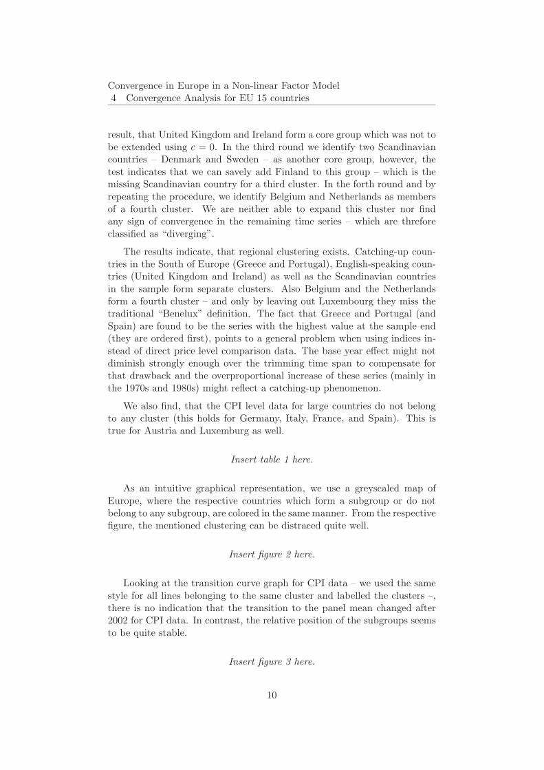
result, that United Kingdom and Ireland form a core group which was not tobe extended using c = 0. In the third round we identify two Scandinaviancountries – Denmark and Sweden – as another core group, however, thetest indicates that we can savely add Finland to this group – which is themissing Scandinavian country for a third cluster. In the forth round and byrepeating the procedure, we identify Belgium and Netherlands as membersof a fourth cluster. We are neither able to expand this cluster nor findany sign of convergence in the remaining time series – which are threforeclassified as “diverging”.

The results indicate, that regional clustering exists. Catching-up coun-tries in the South of Europe (Greece and Portugal), English-speaking coun-tries (United Kingdom and Ireland) as well as the Scandinavian countriesin the sample form separate clusters. Also Belgium and the Netherlandsform a fourth cluster – and only by leaving out Luxembourg they miss thetraditional “Benelux” definition. The fact that Greece and Portugal (andSpain) are found to be the series with the highest value at the sample end(they are ordered first), points to a general problem when using indices in-stead of direct price level comparison data. The base year effect might notdiminish strongly enough over the trimming time span to compensate forthat drawback and the overproportional increase of these series (mainly inthe 1970s and 1980s) might reflect a catching-up phenomenon.

We also find, that the CPI level data for large countries do not belongto any cluster (this holds for Germany, Italy, France, and Spain). This istrue for Austria and Luxemburg as well.

Insert table 1 here.

As an intuitive graphical representation, we use a greyscaled map ofEurope, where the respective countries which form a subgroup or do notbelong to any subgroup, are colored in the same manner. From the respectivefigure, the mentioned clustering can be distraced quite well.


Looking at the transition curve graph for CPI data – we used the samestyle for all lines belonging to the same cluster and labelled the clusters –,there is no indication that the transition to the panel mean changed after2002 for CPI data. In contrast, the relative position of the subgroups seemsto be quite stable.


10


4.3 Results for GDP Deflator and Unit Labor Cost Data

We jointly discuss results for GDP deflator and unit labor cost data jointly,because the results and therefore the conclusions do not differ much. How-ever, compared to the results for CPI data, the results do alter.

First, we present the results for the GDP deflator data set. Using thedata for Spain as the base entity and starting to identify a core group, weidentify a group of five countries – Netherlands, Denmark, Ireland, Austriaand Italy. These countries form the first subgroup. The cluster can easilybe enlarged to contain data for United Kingdom, Greece and Luxemburgas well. So the majority of countries form a first convergence club. In thenext round, the GDP deflator series for Germany is the base series – butthe time series does not belong to the second core group. In fact, we stophere as the data for all remaining countries except Germany form a secondcore group (France, Sweden together with Finland and Belgium). Germanyis divergent as it does not belong to any group.


The results from the unit labor cost data set are qualitatively quite simi-lar. Here again we find that a majority of countries forms a first convergenceclub and a minority of countries forms a second club. France and Swedenare once more members of the second club – but this time accompanied byIreland, Greece and Finland. This time Germany is found to be a memberof the first club in contrast to the results above. The graphs suggest that itmight well be the case that the first convergence club seems to be splittedinto two subclusters since the mid 1990s/ early 2000s – a fact which is notbeen detected by the procedure (yet).


Looking at the respective transition curves (see figure 3) we observe thatremarkable swings, but this holds for the 1980s and 1990s and therefore thistendency seems to be not related to the introduction of the common currency(even if we would allow for announcement effects). A view on the respectivetransition curves for ULC data reveals that within the first sub-group thereis recently a tendency observable to form two separate clusters within thesubgroup. According to that Luxembourg, Germany, Austria and Belgiumseem to form a separate cluster in the last couple of years. Italy is a memberof this subcluster as well but shows some tendency for higher ULC growth.The evidence for subclusters has not yet been detected by the procedureused here but could be a case for further investigation in the next years.

11


4.4 Results for GDP per Capita Data

GDP per capita data show stronger clustering compared to GDP deflatoror unit labor cost data – but the regional structure is more diverse. Theprocedure is applied as before. A cluster of catching-up countries (Irelandand Portugal) is easily identified. A second cluster contains the South-ern countries Greece and Spain but also Luxemburg, Finland, Austria andBelgium. A third cluster is found to be formed by France and some Scandi-navian countries. Germany and Italy do not belong to any of the identifiedclusters.

Looking again at the respective transition curves reveals that in fact,Greece and Portugal seem to have converged, the procedure however hasclustered Portugal with Ireland. Furthermore, there is evidence, that Bel-gium could possibly be better counted as a member of the high-income club.Besides this, there is no evidence for a change in the transition behaviourover the last couple of years.


4.5 Results for Total Factor Productivity Data

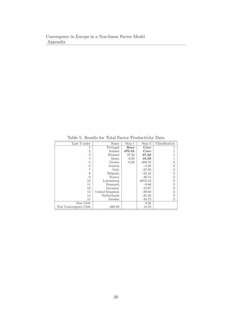
Turning to the analysis of total factor productivity data, the results showquite strong signs of convergence for the majority of countries in the sample.This is a promising result in terms of convergence because throughout thestandard growth theory literature differences in productivity explain thebulk of income convergence in the long-run (Weil, 2004).

Starting with a base country – Portugal here – we define again a coregroup in the first round. The group consists of Portugal and Ireland – twofast-growing countries. In the next step, we again try to add countries tothis group. Finland and Spain pass the test. So we end up with a firstconvergence group – which are mainly catchig-up countries. The procedureis then applied to the rest. Interestingly, all other countries form a conver-gence club in the first test. So we can stop here with the result, that themajority of countries form a convergence club.


The transition curves show that Spain should possibly be counted as amember of the first club and Greece seems to have a tendency to move outof the second club – but again there is no evidence for a change in transitioncurves over the last couple of years.

12

Convergence in Europe in a Non-linear Factor Model5 Conclusion

5 Conclusion

In the paper, we applied a new convergence test procedure on EU 15 datafrom 1960 to present. This procedure is quite general and easily applicableand will definitely become a workhorse of convergence testing within thenext years. In general, our results reveal interesting stylized facts on theconvergence process in Europe.

• Consumer prices suggest clustering along the lines of geographical dis-tance. Countries with common borders as well as strong economicinteractions (Benelux, Scandinvian countries, UK and Ireland) showconvergence. There is no overall convergence.

• GDP deflator and unit labor cost data indicate two clusters: a largegroup of about 2

3 of all countries on the one hand and the rest onthe other hand. Sweden and France always belonged to the secondcluster, other countries differ in their membership. Spain and Germanyare divergent for GDP deflator series. However, there are signs, thatpossibly a change around the mid 1990s /early 2000s occurred whichwould speak in favour of a further subclustering. However, so farevidence for such an event is still quite weak.

• GDP per capita data show the existence of three distinctive clusters:catching-up countries, middle-income countries and high-income coun-tries. Italy and Germany seem to be inconclusive about their mem-bership. For the case of Germany surely the reunification has led toa level shift in per-capita income downwards which makes it difficultfor the procedure to cope with.

• The highest level of convergence is reached in total factor productivity.There is clear evidence for a catching-up cluster and all other countriesseem to form a large cluster. This is the most promising result as itindicates that the long-run prospects for convergence in income andprices can be judged as reasonably good.

13

Convergence in Europe in a Non-linear Factor ModelReferences

References

Alesina, A., and R. Barro (2002): “Currency Unions,” The Quarterly Journal of

Economics, 117, 409 – 436.

Allsopp, C., and M. Artis (2003): “The Assessment: EMU, Four Years On,” Oxford

Review of Economic Policy, 19(1), 1–29.

Altissimo, F., M. Ehrmann, and F. Smets (2006): “Inflation persistence and pricesetting behaviour in the Euro area. A summary of the IPN evidence.,” Occasional PaperSeries 46, European Central Bank.

Angeloni, I., L. Aucremanne, M. Ehrmann, J. Gali, A. Levin, and F. Smets

(2006): “New evidence on inflation persistence and price stickiness in the Euro area:Implications for macro modelling,” Journal of the European Economic Association, 4,562–574.

Angeloni, I., and M. Ehrmann (2004): “Euro area inflation differentials,” WorkingPaper Series 388, European Central Bank.

Bai, J. (2003): “Inferential Theory for Factor Models of Large Dimensions,” Economet-

rica, 71, 135–172.

Barro, R., and X. Sala-i-Martin (1991): “Convergence across states and regions,”Brookings Papers on Economic Activity, 1991(1), 107–182.

(1992): “Convergence,” The Journal of Political Economy, 100(2), 223–251.

Bernard, A. B., and S. N. Durlauf (1996): “Interpreting tests of the convergencehypothesis,” Journal of Econometrics, 71, 161–173.

Busetti, F., L. Forni, A. Harvey, and F. Venditti (2006): “Inflation convergenceand divergence within the European Monetary Union,” ECB Working Paper Series 574,European Central Bank.

Campolmi, A., and E. Faia (2006): “Cyclical inflation divergence and different labormarket institutions in the EMU.,” Working Paper Series 619, European Central Bank.

Cecchetti, S., M. Mark, and R. Sonora (2002): “Price Level Convergence amongUnited States Cities: Lessons for the European Central Bank,” International Economic

Review, 43(4), 1081–1099.

Corsetti, G. (2008): “A Modern Reconsideration of the Theory of Optimal CurrencyAreas,” EUI Working Papers ECO 2008/12, EUI.

Cuaresma, J. C., B. Egert, and M. A. Silgoner (2007): “Price Level Convergence inEurope: Did the Introduction of the Euro Matter?,” Monetary Policy & the Economy,Q1/07, 100–113.

Devereux, M., C. Engel, and C. Tille (2003): “Exchange Rate Pass-through andthe Welfare Effects of the Euro,” International Economic Review, 44(1), 223 – 242.

Durlauf, S. N., and D. T. Quah (1999): Handbook of Macroeconomics. Volume

1A.chap. The New Empirics of Economic Growth, pp. 235–308. Elsevier Science, North-Holland,.

Eichengreen, B. (2007): “The Breakup of the Euro Area,” NBER Working Paper 13393,NBER.

14

Convergence in Europe in a Non-linear Factor ModelReferences

(2008): “Sui Generis EMU,” NBER Working Paper 13740, NBER.

Emerson, M., D. Gros, and A. Italianer (1992): One Market, One Money: An

Evaluation of the Potential Benefits and Costs of Forming an Economic and Monetary

Union. Oxford University Press.

European Central Bank (2003): “Inflation Differentials in the Euro Area: PotentialCauses and Policy Implications,” Discussion paper, European Central Bank.

Hobijn, B., and P. H. Franses (2000): “Asymptotically perfect and relative conver-gence of productivity,” Journal of Applied Econometrics, 15, 59–81.

Islam, N. (2003): “What have we learnt from the convergence debate,” Journal of Eco-

nomic Surveys, 17(3), 309–362.

Lane, P. (2006): “The real effects of EMU,” Discussion Paper Series 5536, CEPR.

Melander, A., G. Sismanidis, and D. Grenouilleau (2007): “The track of the Com-mission’s forecast: an update,” European Economy. Economic Papers 291, EuropeanCommission.

Phillips, P. C. B. (2005): “Challenges of Trending Time Series Econometrics,” Mathe-

matics and Computers in Simulation, 68, 401–416.

Phillips, P. C. B., and D. Sul (2007): “Transition modelling and econometric conver-gence tests,” Econometrica, 75, 1771 – 1855.

Rose, A. (2000): “One money, one market: the effect of common currencies on trade,”Economic Policy, 30, 7 – 45.

Rose, A., and C. Engel (2002): “Currency Unions and International Integration,”Journal of Money, Credit, and Banking,, 34(4), 1067–1086.

Tenreyro, S., and R. Barro (2007): “Economic Effects of Currency Unions,” Eco-

nomic Inquiry, 45(1), 1–197.

Weil, D. N. (2004): Economic growth. Addison Wesley.

15

Convergence in Europe in a Non-linear Factor ModelAppendix

Appendix

.12

.16

.20

.24

.28

.32

1995

1996

1997

1998

1999

2000

2001

2002

2003

2004

2005

Source: Eurostat

Figure 1: Cross-section distribution of coefficients of variation in EU 15,1995-2005, measured against EU 15 average, 41 product categories in eaxhcountry, Source: Eurostat

16

Con

vergen

cein

Europ

ein

aN

on-lin

earFactor

Model

Appen

dix

Table 1: Results for CPI data

Last T order Name Step 1 Step 2 Step 1 Step 2 Step 1 Step 2 Step 1 Step 2 Step 1 Classification

1 Greece Base Core 12 Portugal 4.48 Core 13 Spain -94.99 -94.99 Base -28.79 Base -351.68 Base -18.24 Base divergence4 Italy -612.21 -134.72 -15.96 -134.72 -57.46 -134.72 -13.49 -134.72 divergence5 Ireland -606.31 -3.71 Core 26 United Kingdom -34.22 26.61 Core 27 Finland -53.74 -74.80 -74.80 -23.01 32.51 38 Denmark -39.84 -61.21 -5.66 Core 39 Sweden -43.77 -48.18 27.80 Core 3

10 France -68.39 -373.42 -4.03 -4.03 -120.02 -3.19 -120.02 divergence11 Belgium -27.95 -44.56 -33.97 -4.98 Core 412 Netherlands -16.73 -11.96 -7.47 -0.70 Core 413 Luxemburg -28.22 -34.78 -27.60 -19.34 -19.34 -5.18 divergence14 Austria -20.65 -28.10 -11.13 -13.73 -2.69 divergence15 Germany -19.60 -25.96 -12.03 -32.82 -16.92 divergence

Test Club 32.51Test Convergence Club -26.61 -18.10 -16.82 -17.23 -18.70

17


Table 2: Results for GDP Deflator Data

Last T order Name Step 1 Step 2 Step 1 Step 2 Classification

1 Spain Base -16.54 Base -147.83 divergence2 Netherlands -3.78 Core 13 Denmark 1.53 Core 14 Ireland 35.84 Core 15 Austria 20.21 Core 16 Italy 71.80 Core 17 Portugal 11.14 11.14 18 United Kingdom 9.71 8.03 19 Greece 8.36 8.91 1

10 Germany 8.47 -1.62 -65.68 -14.40 divergence11 Luxemburg 7.20 8.61 112 Finland 10.93 -12.62 -28.62 Core 213 Belgium 16.41 -242.10 10.81 Core 214 France 27.71 -30.17 7.84 Core 215 Sweden -17.2594 -16.7756 13.65 Core 2

Test Club 7.49Test Convergence Club -22.93 -260.66 -65.68

Table 3: Results for Unit Labor Cost Data

Last T order Name Step 1 Step 2 Classification

1 Spain Base Core 12 Netherlands -1.18 Core 13 Denmark 0.12 Core 14 United Kingdom 6.39 Core 15 Portugal 7.74 Core 16 Luxemburg 6.81 Core 17 Austria 11.18 Core 18 Germany 29.55 Core 19 Italy 21.09 Core 1

10 Belgium 36.75 Core 111 Ireland -4.04 -4.04 112 France -87.69 213 Sweden -19.40 214 Finland -62.31 215 Greece -0.02 2

Test ClubTest Convergence Club 48.83 10.19

18

Con

vergen

cein

Europ

ein

aN

on-lin

earFactor

Model

Appen

dix

Table 4: Results for GDP per Capita Data

Last T order Name Step 1 Step 2 Step 1 Step 2* Step 1 Step 2 Classification

1 Ireland Base Core 12 Portugal 2.08 Core 13 Greece -7.20 -7.20 Base Core 24 Spain -27.35 1.8096 Core 25 Luxemburg -33.84 49.0264 Core 26 Finland -30.38 108.344 Core 27 Austria -33.32 38.06 38.06 28 Italy -30.52 6.66 7.52 Base -8.36 divergence9 Belgium -26.99 -36.44 11.75 2

10 France -24.16 -5.10 -12.11 Core 311 Denmark -23.77 -6.37 102.04 Core 312 Netherlands -86.12 -16.95 8.96 8.96 313 Sweden -5841.59 -4.87 2.68 0.12 314 United Kingdom -39.85 -11.02 12.02 171.47 315 Germany -35.89 -6.03 -13.05 -40.64 divergence

Test Club -0.14Test Convergence Club -14.00 -18.37 -16.62 -37.91

Legend: * We increased c unless the tb

> −1.65, which was achieved at c = 8.

19


Table 5: Results for Total Factor Productivity Data

Last T order Name Step 1 Step 2 Classification

1 Portugal Base Core 12 Ireland 470.55 Core 13 Finland 37.22 37.22 14 Spain 6.56 16.39 15 Greece -9.20 -400.55 26 Austria -5.39 27 Italy -27.03 28 Belgium -22.44 29 France -46.74 2

10 Luxemburg -2012.43 211 Denmark -9.86 212 Germany -13.07 213 United Kingdom -30.60 214 Netherlands -25.40 215 Sweden -34.73 2

Test Club 6.56Test Convergence Club -268.89 14.70

20


Figure 2: Regional Clustering

(a) log(CPI) (b) log(Deflator)

(c) log(Unit Labor Costs) (d) log(GDP)

(e) log(TFP)

21


Figure 3: Transition Curves

1975 1980 1985 1990 1995 2000 2005

0.9

1.0

1.1

1.2 C1

C2

C3

C4

(a) log(CPI)

1975 1980 1985 1990 1995 2000 2005

0.950

0.975

1.000

1.025

1.050

C1

C2

(b) log(Deflator)

1975 1980 1985 1990 1995 2000 2005

0.900

0.925

0.950

0.975

1.000

1.025

1.050

1.075 C1

C2

(c) log(Unit Labor Costs)

1975 1980 1985 1990 1995 2000 2005

0.950

0.975

1.000

1.025

1.050

1.075

1.100

C1

C2

C3

(d) log(GDP)

1975 1980 1985 1990 1995 2000 2005

0.975

1.000

1.025

1.050

1.075

C1

C2

(e) log(TFP)

22

Documents

Analysing Convergence in Europe Using a Non-linear Single