Embed Size (px)
Citation preview
2
Index
Definition of an analog computer
Mechanical analog calculators & computers
Electronic analog computers
Demonstrations
The future. Literature and links

3
Definition
An analog computer works in a continuous manner
(a digital computer functions in discrete steps).
An analog computer uses a model which behaves in
a similar way (= in an “analog” way) to the problem
to be solved.
The oldest analog computers were purely
mechanical systems, later systems were
electronic devices.
4
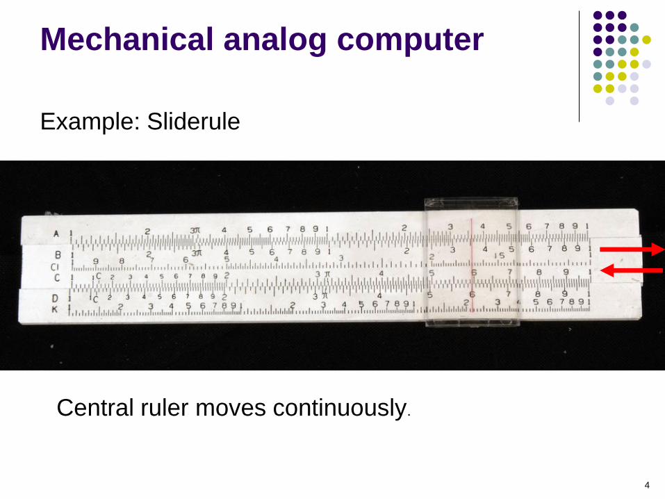
Mechanical analog computer
Example: Sliderule
Central ruler moves continuously.
5
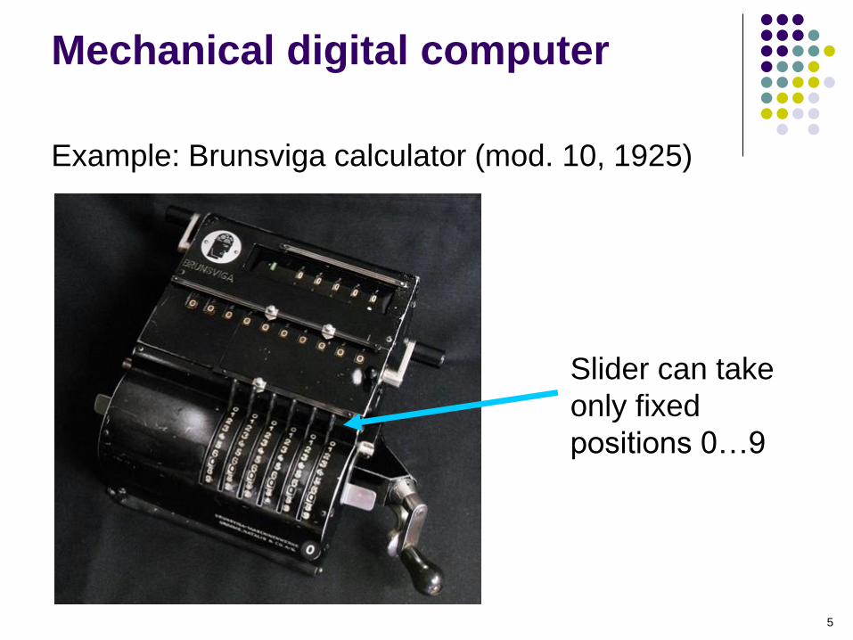
Mechanical digital computer
Example: Brunsviga calculator (mod. 10, 1925)
Slider can take
only fixed
positions 0…9

6
Mechanical analog computer
Antikythera, 78 BC (astrolabe)
Oldest analog computer known:
at least 30 gears!
(found in 1900 by sponge divers)
Several rebuilds since 1978
(Antikythera Mechanism Research
project)
7
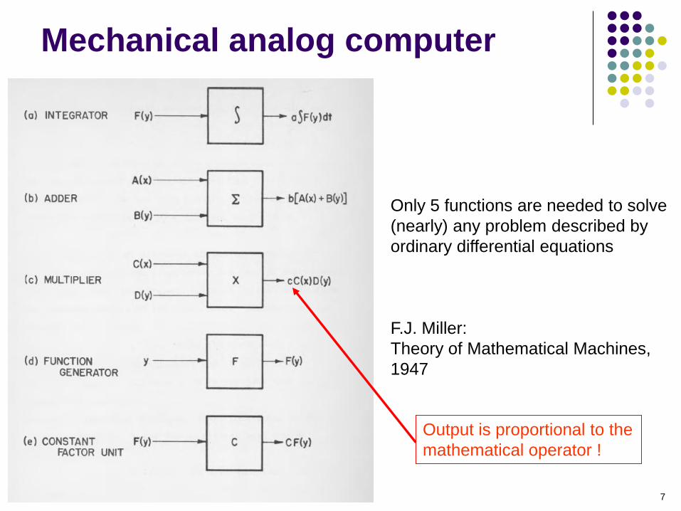
Mechanical analog computer
Only 5 functions are needed to solve
(nearly) any problem described by
ordinary differential equations
F.J. Miller:
Theory of Mathematical Machines,
1947
Output is proportional to the
mathematical operator !
8
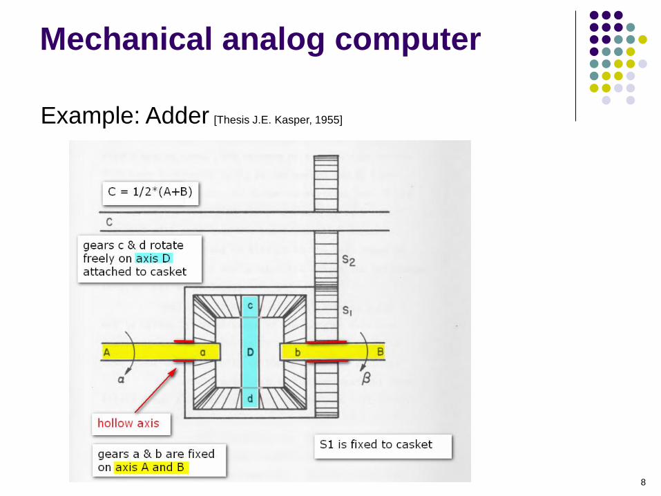
Mechanical analog computer
Example: Adder [Thesis J.E. Kasper, 1955]

9
Mechanical analog computer
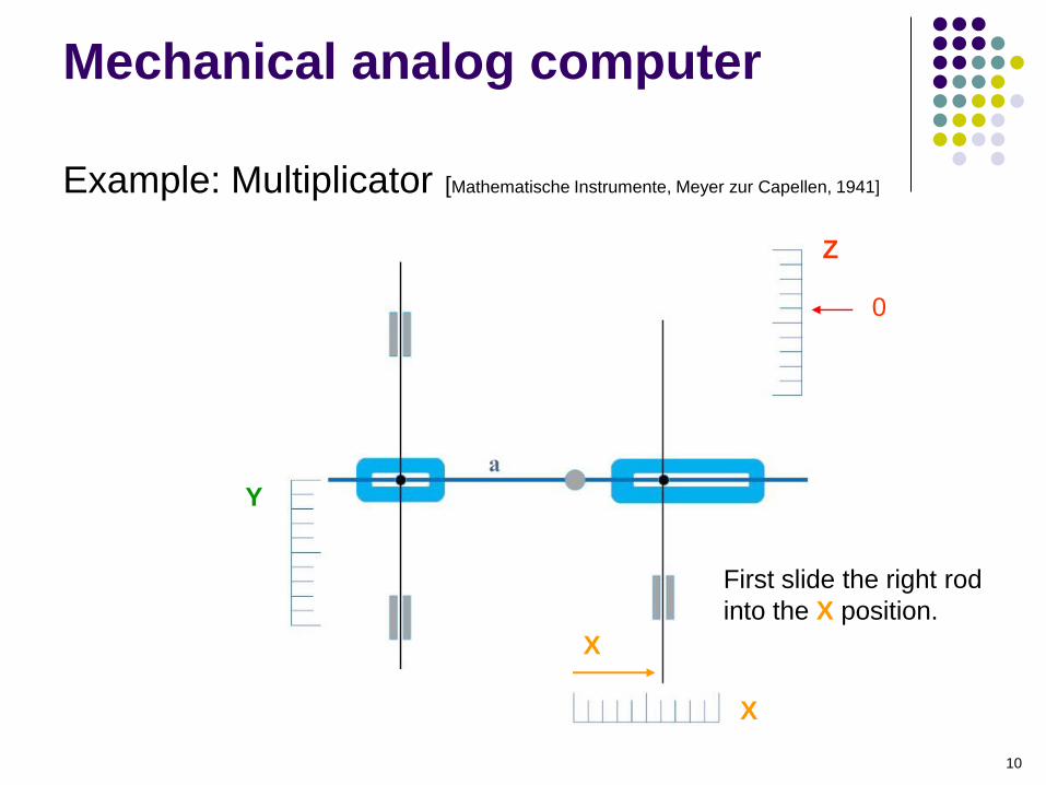
Example: Multiplicator [Mathematische Instrumente, Meyer zur Capellen, 1941]
Y
X
The black knob is fixed
on the vertical rods, but
slides on the horizontal
level.
Z
10
Mechanical analog computer
Example: Multiplicator [Mathematische Instrumente, Meyer zur Capellen, 1941]
Y
X
0
First slide the right rod
into the X position.
X
Z
X

11
Mechanical analog computer
Example: Multiplicator [Mathematische Instrumente, Meyer zur Capellen, 1941]
Y
X
Z
Now push the left rod
down into
the Y position
X
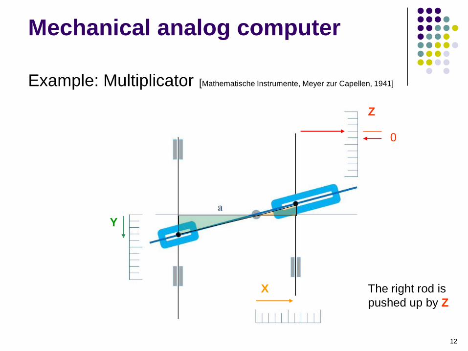
The right rod is
pushed up by Z
X
0
12
Mechanical analog computer
Example: Multiplicator [Mathematische Instrumente, Meyer zur Capellen, 1941]
Y
X
Z
X
The right rod is
pushed up by Z
X
0
13
Mechanical analog computer
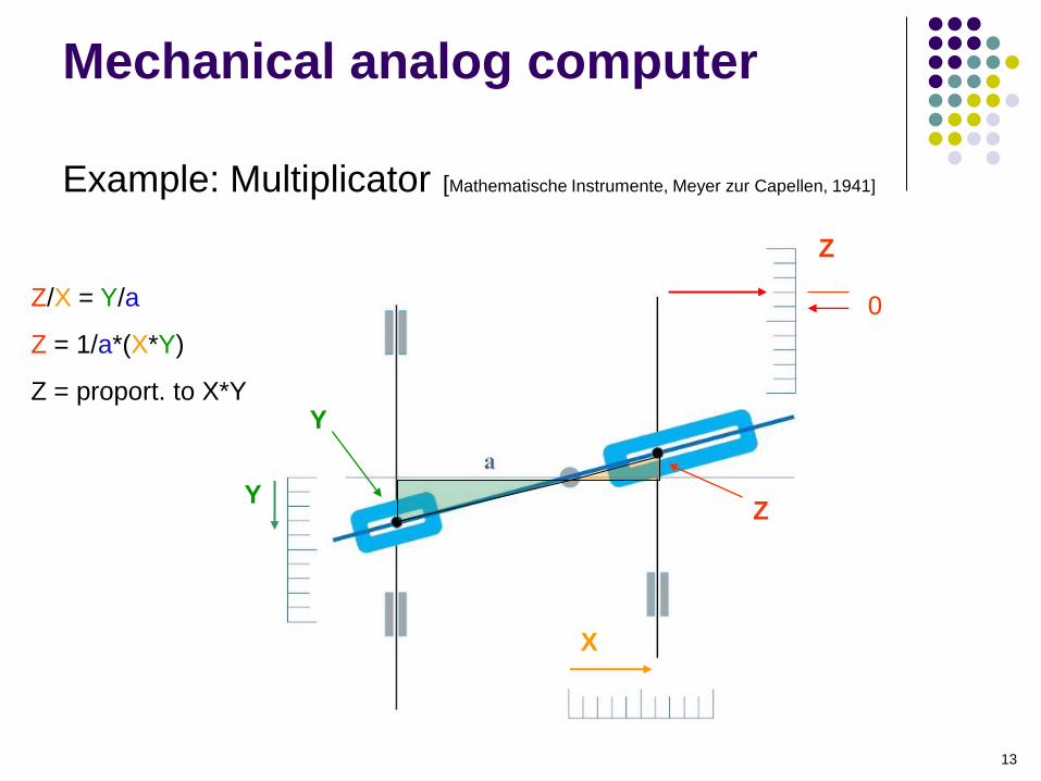
Example: Multiplicator [Mathematische Instrumente, Meyer zur Capellen, 1941]
Y
X
Z
X
X
0
Z
Y
Z/X = Y/a
Z = 1/a*(X*Y)
Z = proport. to X*Y

14
Military screw multiplier
From ordnance
pamphlet 1140
Gun and Fire control
(US Navy)
http://archive.hnsa.org/
15
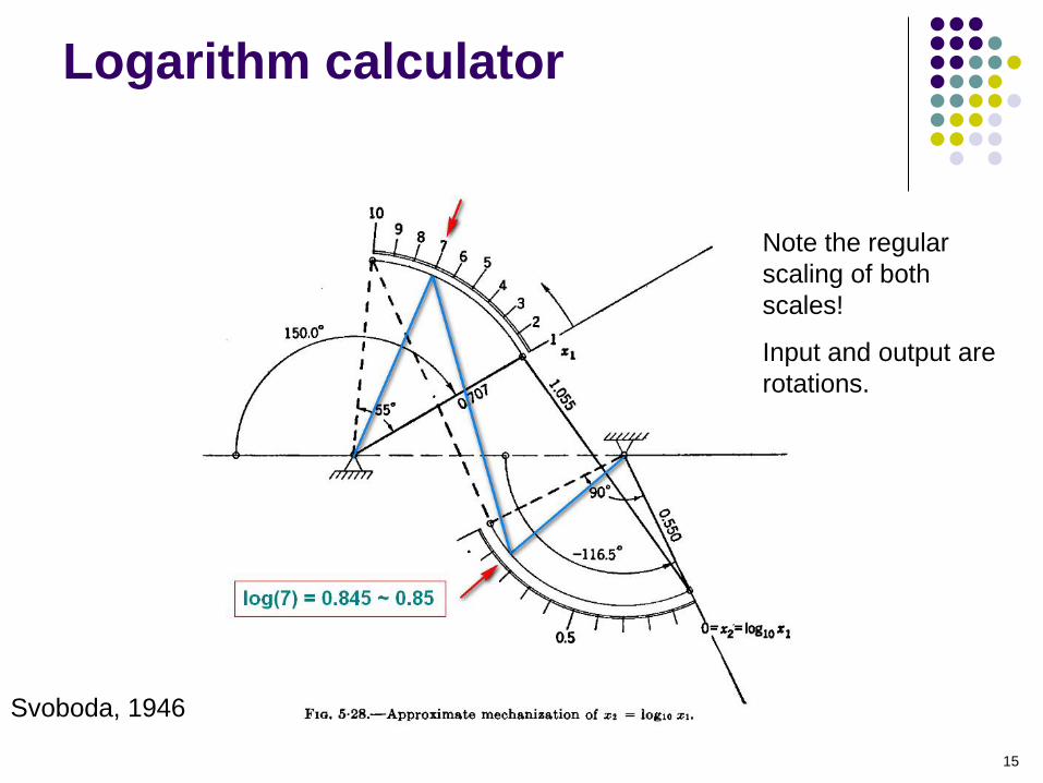
Logarithm calculator
Svoboda, 1946
Note the regular
scaling of both
scales!
Input and output are
rotations.
16
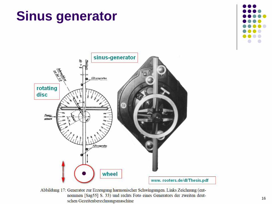
Sinus generator
17
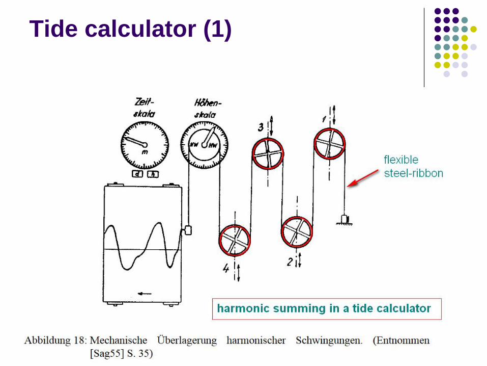
Tide calculator (1)
18
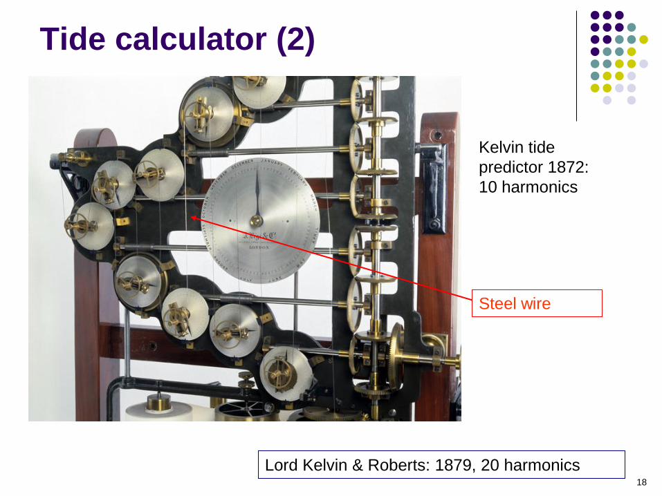
Tide calculator (2)
Lord Kelvin & Roberts: 1879, 20 harmonics
Kelvin tide
predictor 1872:
10 harmonics
Steel wire
19
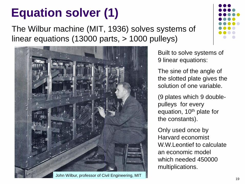
Equation solver (1)
The Wilbur machine (MIT, 1936) solves systems of
linear equations (13000 parts, > 1000 pulleys)
Built to solve systems of
9 linear equations:
The sine of the angle of
the slotted plate gives the
solution of one variable.
(9 plates which 9 double-
pulleys for every
equation, 10th plate for
the constants).
Only used once by
Harvard economist
W.W.Leontief to calculate
an economic model
which needed 450000
multiplications.
John Wilbur, professor of Civil Engineering, MIT

20
Equation solver (2)
One plate of the Wilbur machine:
9 slots: one for
each variable
10th slot to
read sin(angle)
Micrometer screw to
move the pulley (set
the coefficient)
Wilbur machine: time to solve a system
~1 to 3 hours. Without the machine
Leontief’s model would have needed
2 years at 120 multiplications/hour
21
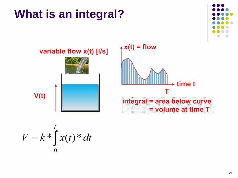
What is an integral?

22
Integrators: planimeter
Made from approx. 1850 - 1970
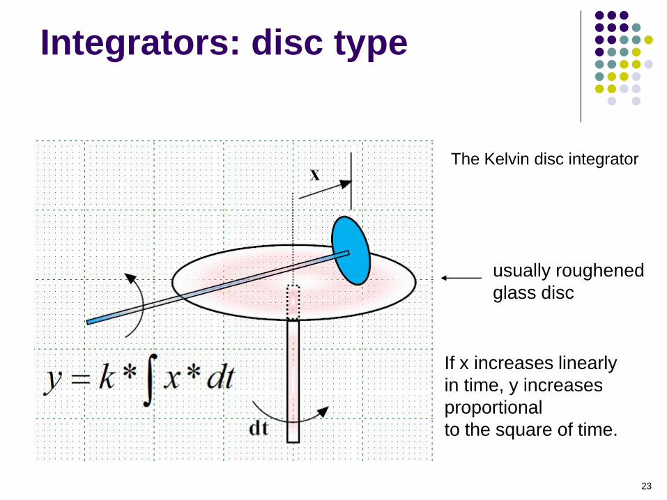
23
Integrators: disc type
usually roughened
glass disc
If x increases linearly
in time, y increases
proportional
to the square of time.
The Kelvin disc integrator
24
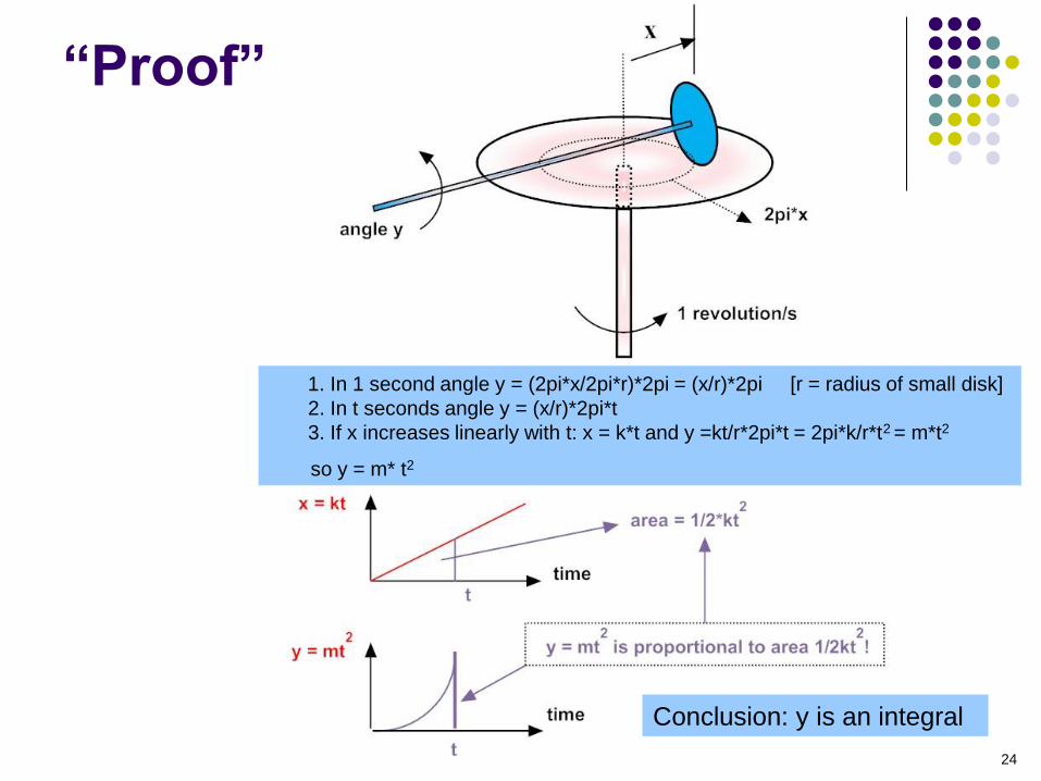
“Proof”
1. In 1 second angle y = (2pi*x/2pi*r)*2pi = (x/r)*2pi [r = radius of small disk]
2. In t seconds angle y = (x/r)*2pi*t
3. If x increases linearly with t: x = k*t and y =kt/r*2pi*t = 2pi*k/r*t2 = m*t2
so y = m* t2
Conclusion: y is an integral
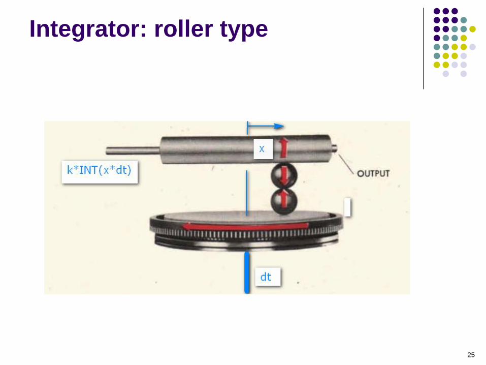
25
Integrator: roller type
26
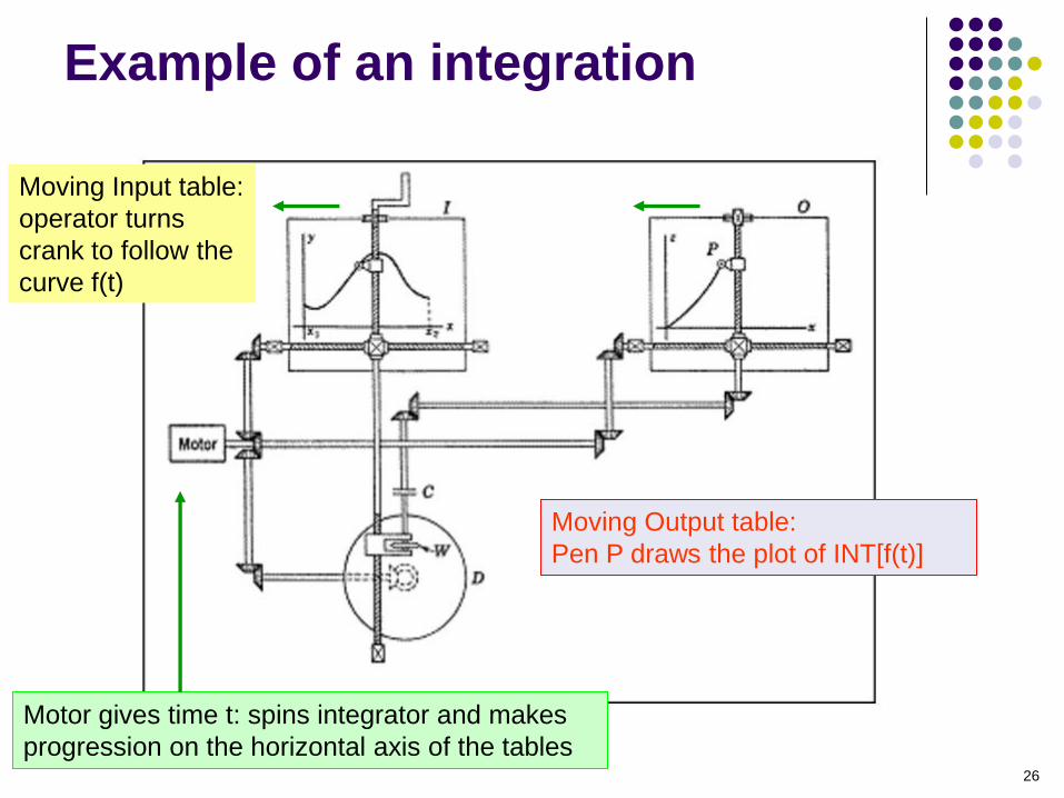
Example of an integration
Motor gives time t: spins integrator and makes
progression on the horizontal axis of the tables
Moving Input table:
operator turns
crank to follow the
curve f(t)
Moving Output table:
Pen P draws the plot of INT[f(t)]
27
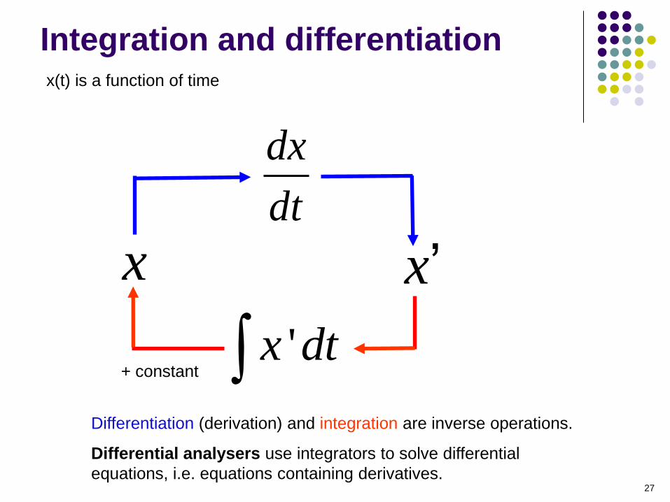
Integration and differentiation
dx
dt
x x’
'x dtDifferentiation (derivation) and integration are inverse operations.
Differential analysers use integrators to solve differential
equations, i.e. equations containing derivatives.
+ constant
x(t) is a function of time
28
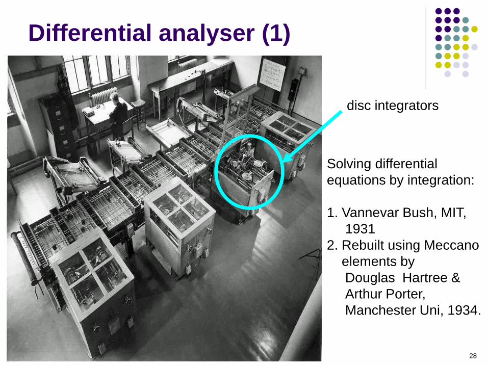
Differential analyser (1)
Solving differential
equations by integration:
1. Vannevar Bush, MIT,
1931
2. Rebuilt using Meccano
elements by
Douglas Hartree &
Arthur Porter,
Manchester Uni, 1934.
disc integrators
29
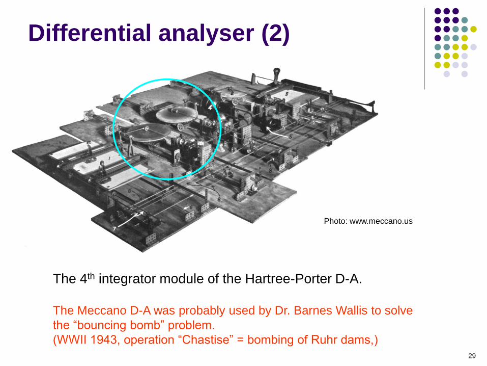
Differential analyser (2)
The 4th integrator module of the Hartree-Porter D-A.
The Meccano D-A was probably used by Dr. Barnes Wallis to solve
the “bouncing bomb” problem.
(WWII 1943, operation “Chastise” = bombing of Ruhr dams,)
Photo: www.meccano.us
30
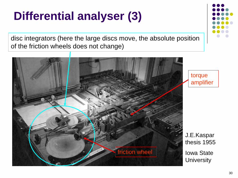
Differential analyser (3)
disc integrators (here the large discs move, the absolute position
of the friction wheels does not change)
J.E.Kaspar
thesis 1955
Iowa State
University
friction wheel
torque
amplifier
31
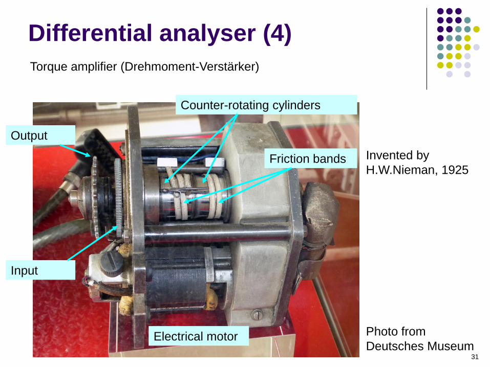
Differential analyser (4)
Torque amplifier (Drehmoment-Verstärker)
Output
Input
Electrical motor
Counter-rotating cylinders
Friction bands Invented by
H.W.Nieman, 1925
Photo from
Deutsches Museum
32
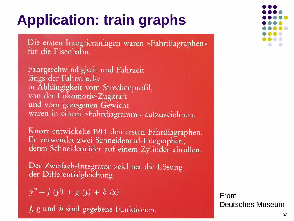
Application: train graphs
From
Deutsches Museum

33
Conzen-Ott “Fahrzeitrechner”
Function-
generator h(x)
Spherical calotte integrator
Output graph
Introduced in 1943.
In use at the
Deutsche Bahn
up into the 1980’s.
Photo from
Deutsches Museum
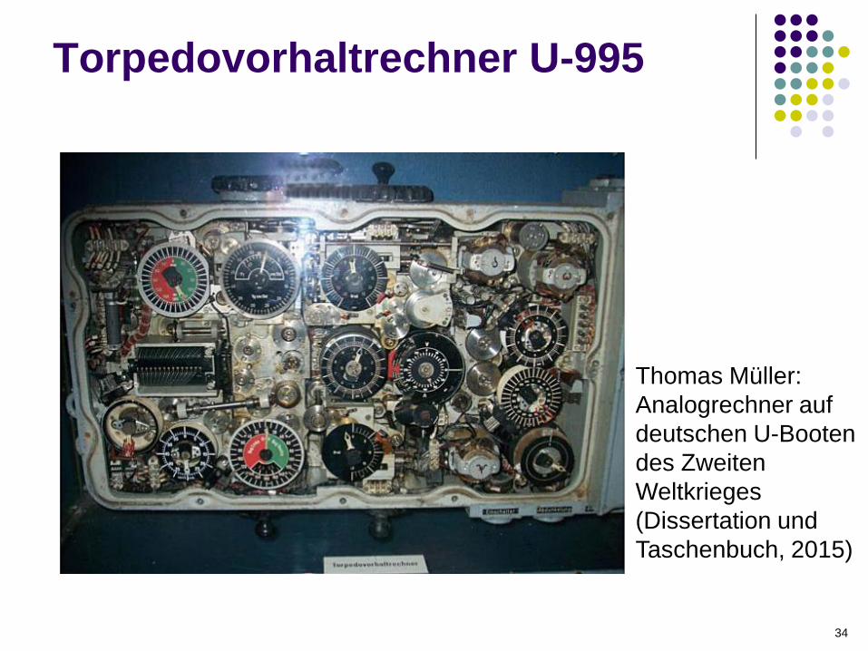
34
Torpedovorhaltrechner U-995
Thomas Müller:
Analogrechner auf
deutschen U-Booten
des Zweiten
Weltkrieges
(Dissertation und
Taschenbuch, 2015)
35
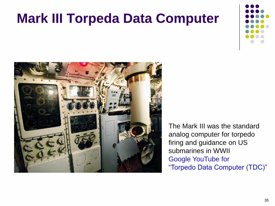
Mark III Torpeda Data Computer
The Mark III was the standard
analog computer for torpedo
firing and guidance on US
submarines in WWII
Google YouTube for
“Torpedo Data Computer (TDC)”
36
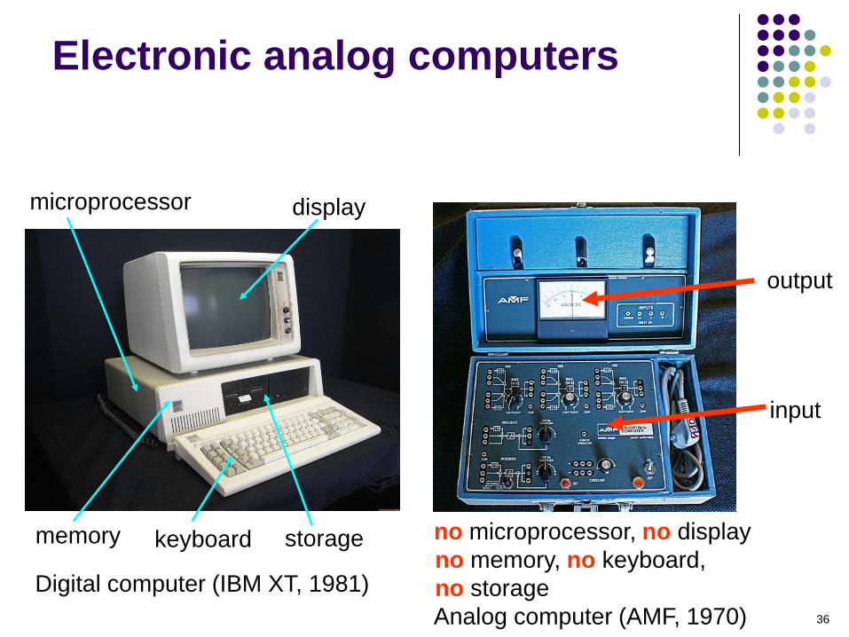
Electronic analog computers
display
keyboard storage memory
microprocessor
Digital computer (IBM XT, 1981)
no microprocessor, no display
no memory, no keyboard,
no storage
Analog computer (AMF, 1970)
output
input

37
One fundamental component: the
Operation Amplifier (OA)
- Voltage amplifier with very high gain (typ. 100000 to 1000000)
- usually –input is used, output voltage is inverted
- input current virtually 0
- two supply voltages Vss, typical +15 and -15 VDC
38
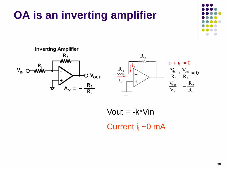
OA is an inverting amplifier
Vout = -k*Vin
Current ii ~0 mA
39
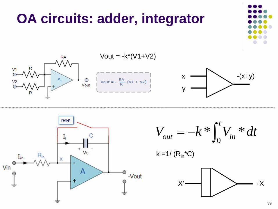
OA circuits: adder, integrator
Vout = -k*(V1+V2)
x
y
-(x+y)
0* *
t
out inV k V dt k =1/ (Rin*C)
X’ -X

40
Example of integration
Vin
time
a
time
-Vout
41
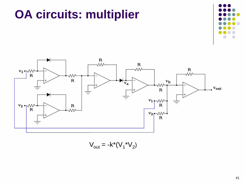
OA circuits: multiplier
Vout = -k*(V1*V2)

42
History of OA’s (1)
Helmut Hoelzer,
Peenemünde, 1941
Germany
K2-GW
first commercial OA
G.A. Philbrick, 1952
USA
1 dual triode
1 pentode/triode
2 triodes
43
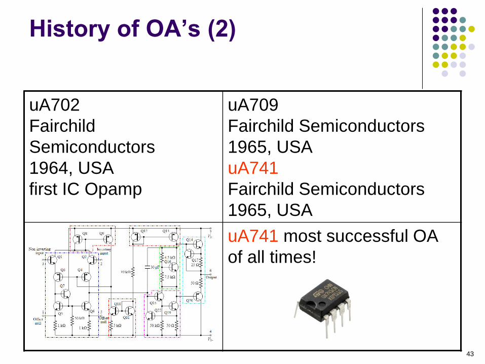
History of OA’s (2)
uA702
Fairchild
Semiconductors
1964, USA
first IC Opamp
uA709
Fairchild Semiconductors
1965, USA
uA741
Fairchild Semiconductors
1965, USA
uA741 most successful OA
of all times!
44
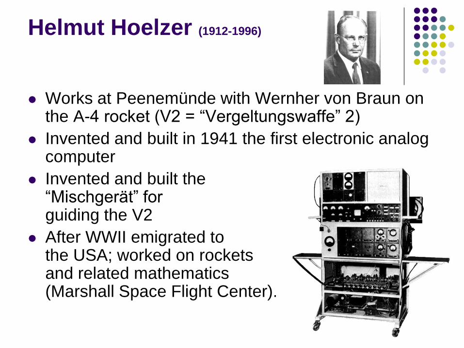
Helmut Hoelzer (1912-1996)
Works at Peenemünde with Wernher von Braun on the A-4 rocket (V2 = “Vergeltungswaffe” 2)
Invented and built in 1941 the first electronic analog computer
Invented and built the “Mischgerät” for guiding the V2
After WWII emigrated to the USA; worked on rockets and related mathematics (Marshall Space Flight Center).
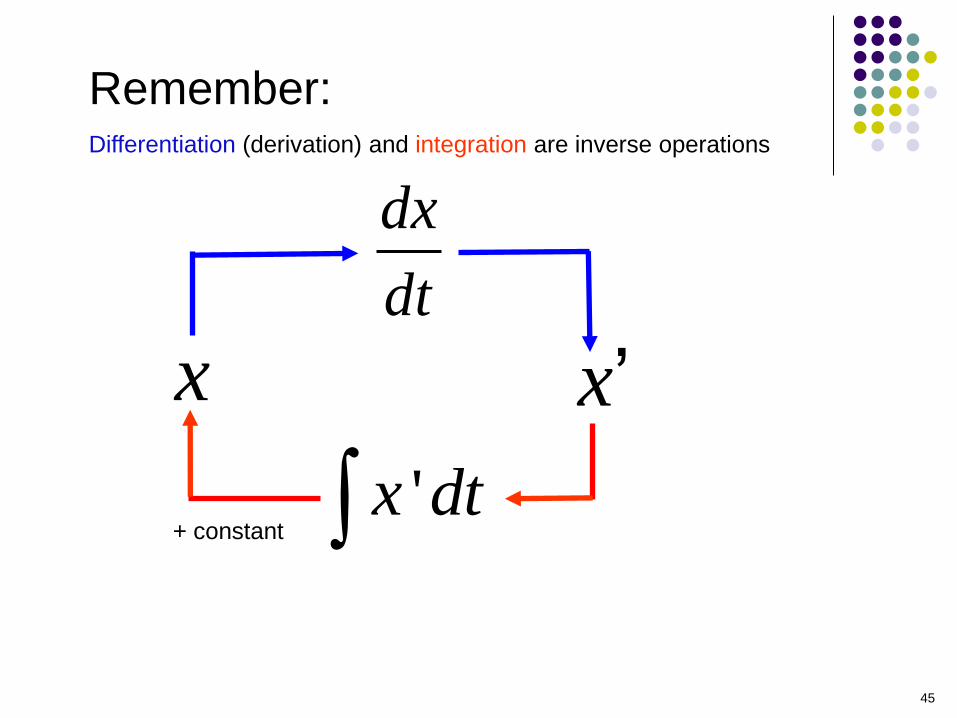
45
dx
dt
x x’
'x dt
Remember: Differentiation (derivation) and integration are inverse operations
+ constant
46
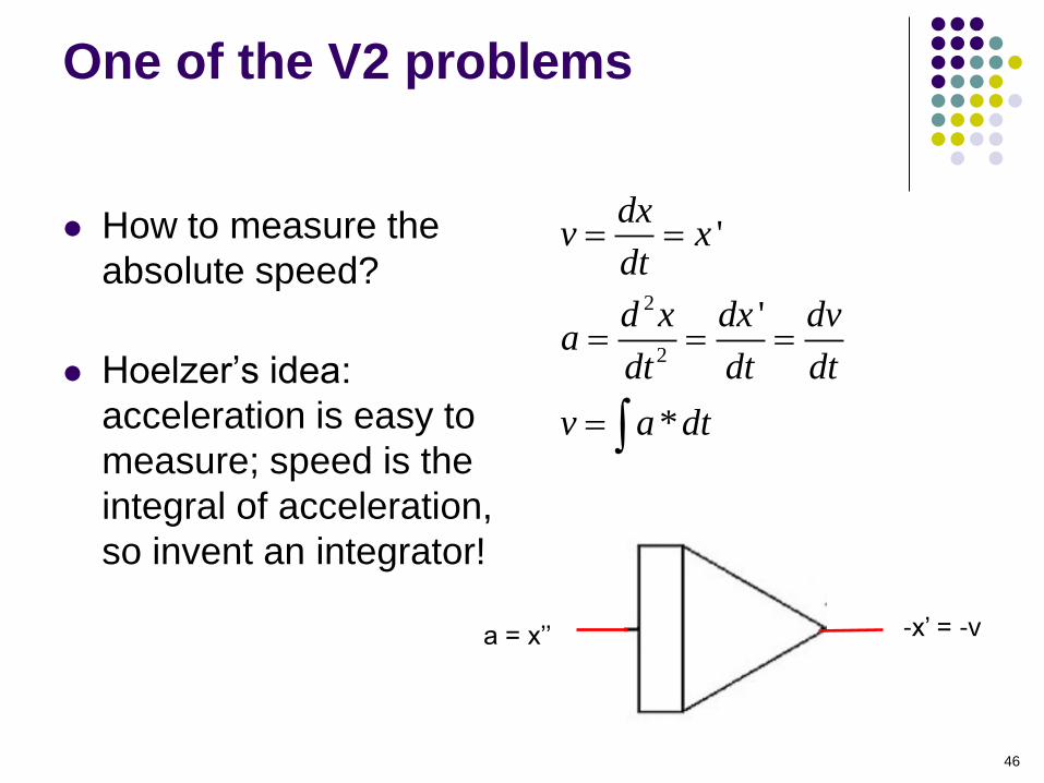
One of the V2 problems
How to measure the
absolute speed?
Hoelzer’s idea:
acceleration is easy to
measure; speed is the
integral of acceleration,
so invent an integrator!
2
2
'
'
*
dxv x
dt
d x dx dva
dt dt dt
v a dt
a = x’’ -x’ = -v
47
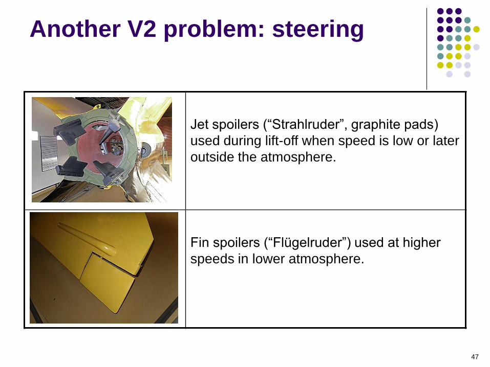
Another V2 problem: steering
Jet spoilers (“Strahlruder”, graphite pads)
used during lift-off when speed is low or later
outside the atmosphere.
Fin spoilers (“Flügelruder”) used at higher
speeds in lower atmosphere.
48
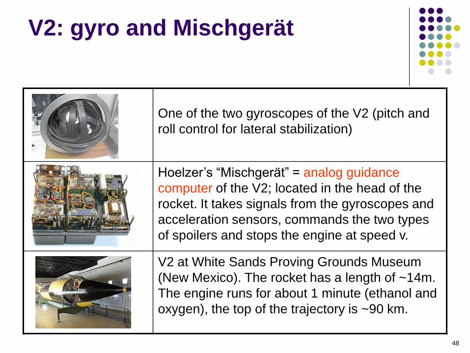
V2: gyro and Mischgerät
One of the two gyroscopes of the V2 (pitch and
roll control for lateral stabilization)
Hoelzer’s “Mischgerät” = analog guidance
computer of the V2; located in the head of the
rocket. It takes signals from the gyroscopes and
acceleration sensors, commands the two types
of spoilers and stops the engine at speed v.
V2 at White Sands Proving Grounds Museum
(New Mexico). The rocket has a length of ~14m.
The engine runs for about 1 minute (ethanol and
oxygen), the top of the trajectory is ~90 km.
49
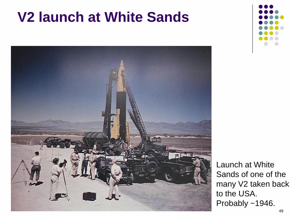
V2 launch at White Sands
Launch at White
Sands of one of the
many V2 taken back
to the USA.
Probably ~1946.
50
Analog (electronic) computer
Uses a model of the process to be solved. Variable structure, depending on program!
Application: process control and simulation: chemical and nuclear reactors, flight, fluid flow, epidemics…
Mostly used from 1950 to about 1970’s
Works in real time and in parallel, up to 100000 times faster than the first digital computers

51
Some examples
of analog computer manufacturers
EAI (Electronic Associates Incorporated, New Jersey, USA, *1945)
European headquarter in Brussels. First analog computer in 1952.
EAI (Pace) 231R
Computer, 1961
Patch panel for
programming
Plotter for output
Pierre DAVID, a
former LCD
student, worked
at EAI, Brussels.

52
EAI analog computers (2)
Assembly line http://www.joostrekveld.net
53
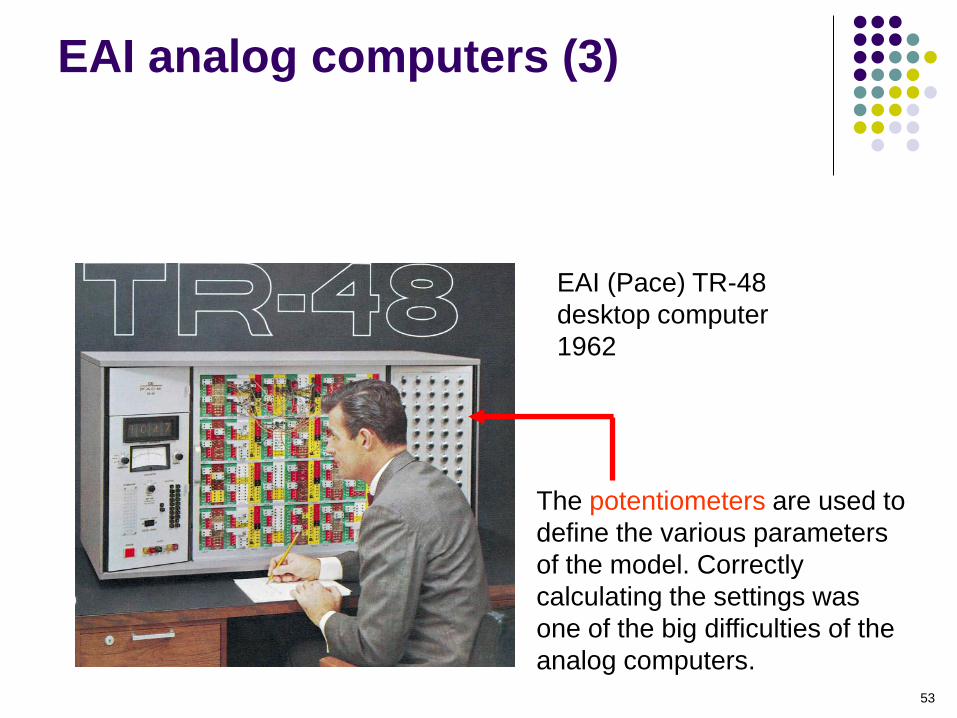
EAI analog computers (3)
EAI (Pace) TR-48
desktop computer
1962
The potentiometers are used to
define the various parameters
of the model. Correctly
calculating the settings was
one of the big difficulties of the
analog computers.
54
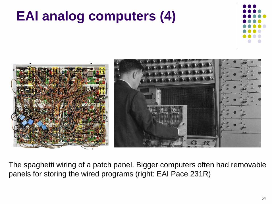
EAI analog computers (4)
The spaghetti wiring of a patch panel. Bigger computers often had removable
panels for storing the wired programs (right: EAI Pace 231R)
55
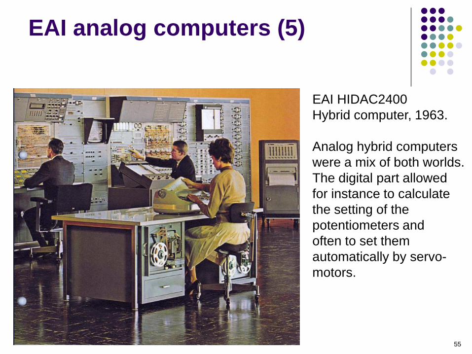
EAI analog computers (5)
EAI HIDAC2400
Hybrid computer, 1963.
Analog hybrid computers
were a mix of both worlds.
The digital part allowed
for instance to calculate
the setting of the
potentiometers and
often to set them
automatically by servo-
motors.
56
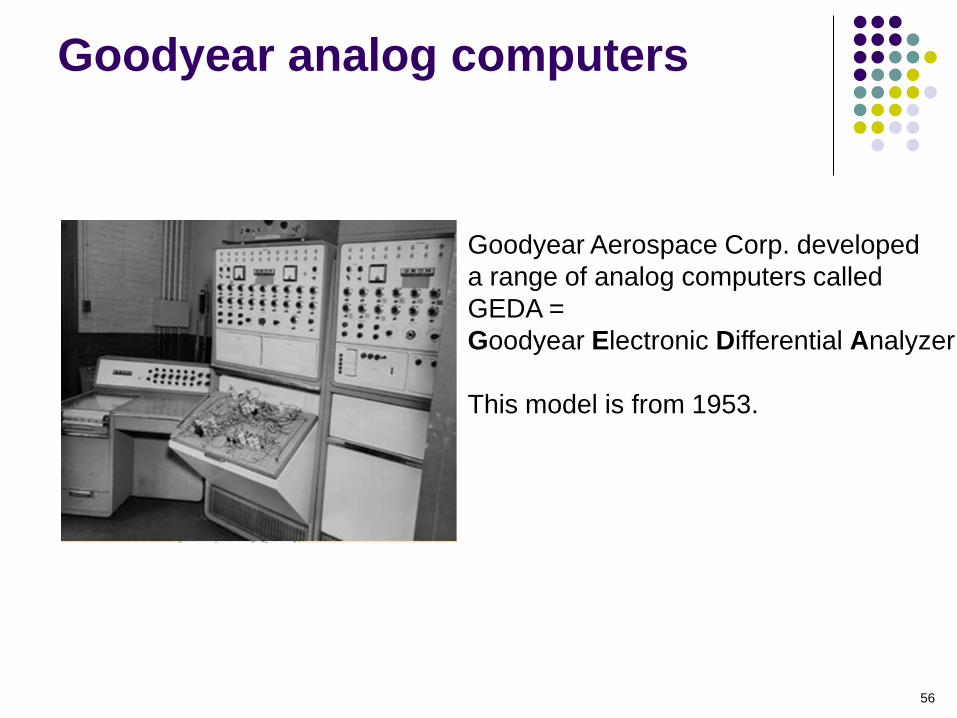
Goodyear analog computers
Goodyear Aerospace Corp. developed
a range of analog computers called
GEDA =
Goodyear Electronic Differential Analyzer
This model is from 1953.

57
Dornier analog computers
The aircraft constructor DORNIER (DE)
started building analog computers to solve
the problems related to VTOL planes
(DO-31 E3, first flight 1967)
Dornier DO-240
analog computer (~1970) (www.technikum29.de)

58
Telefunken analog computers (1)
Telefunken RA-1
First analog computer built
by Telefunken in 1955.
(photo Prof. Bernd Ulmann)
Two oscilloscopes to
visualize the results
59
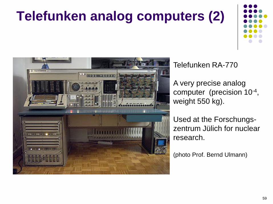
Telefunken analog computers (2)
Telefunken RA-770
A very precise analog
computer (precision 10-4,
weight 550 kg).
Used at the Forschungs-
zentrum Jülich for nuclear
research.
(photo Prof. Bernd Ulmann)

60
analog
computers (1)
Heathkit EC-1
Educational computer
1961, 9 OA with tubes
The R,C components to define the function (adder,
integrator,…) must be added on the front-plane.
Precision and stability are modest.

61
analog
computers (2)
AMF
(American Machine and Foundry:
bowling, bicycles, tennis rackets,
nuclear reactors for research…)
AMF 665/D educational computer
from 1970.
OA = u741
2 integrators, 3 adders
(donated by AALCD).

62
analog
computers (3) COMDYNA GP-6
6 integrators, 2 multipliers, 2 inverters. Built from 1968 to 2004. OA = u741.
Comdyna founder is Ray Spiess, a former EAI engineer.
This specimen comes from the University of Wisconsin (donated by AALCD).

63
Solving the damped oscillator
problem (1)
spring viscous damping:
damping force is
proportional to velocity
To solve this problem we need a model!
x
m

64
Solving the damped oscillator
problem (2)
Spring force = -k*x damping force = - d*v = - d*x’
Total force = -k*x - d*x’
Newton: Total force = m*a = m*x’’ m*x’’ = -d*x’ – k*x
x
For simplicity: m = d = k = 1: x’’ = -x’ - x
this is the model!
x(t) is the solution to find…
65
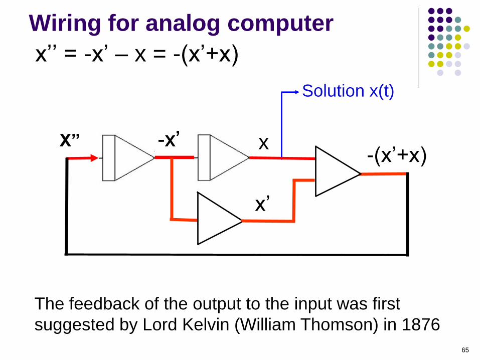
Wiring for analog computer
x’’ = -x’ – x = -(x’+x)
-x’ X’’ -x’ -x’ -x’
x’
Solution x(t)
x -(x’+x)
The feedback of the output to the input was first
suggested by Lord Kelvin (William Thomson) in 1876
66
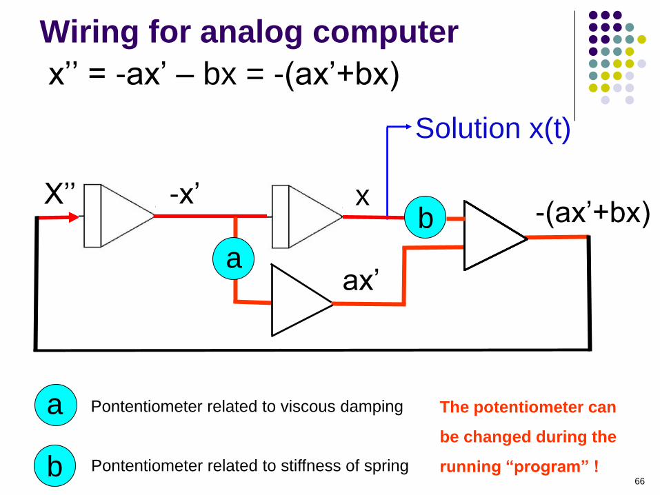
Wiring for analog computer
x’’ = -ax’ – bx = -(ax’+bx)
X’’ X’’ X’’ X’’ -x’
ax’
Solution x(t)
x -(ax’+bx)
a
b
a
b
Pontentiometer related to viscous damping
Pontentiometer related to stiffness of spring
The potentiometer can
be changed during the
running “program” !
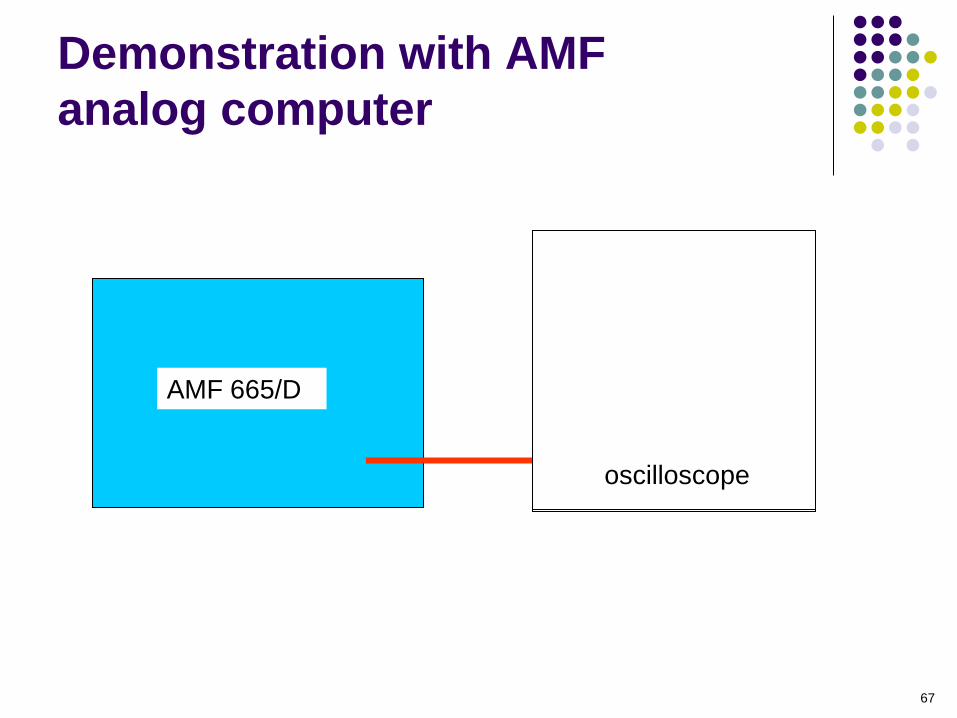
67
Demonstration with AMF
analog computer
AMF 665/D
oscilloscope oscilloscope

68
An “infectious problem” (1)
Town has population of 1000
Initially: 10 are sick (y) 900 may be become sick (x) 90 are immune (z)
Contact rate between sick and not yet sick people = 1/1000 (per day)
1/14 of the sick become immune every day
How do x, y, z evolve in time?

69
An “infectious problem” (2)
Contact rate between sick and not yet sick people =
1/1000 (per day):
x’ = - 1/1000*(x*y) [ change per day of
not yet sick people ]
new infections per day
70
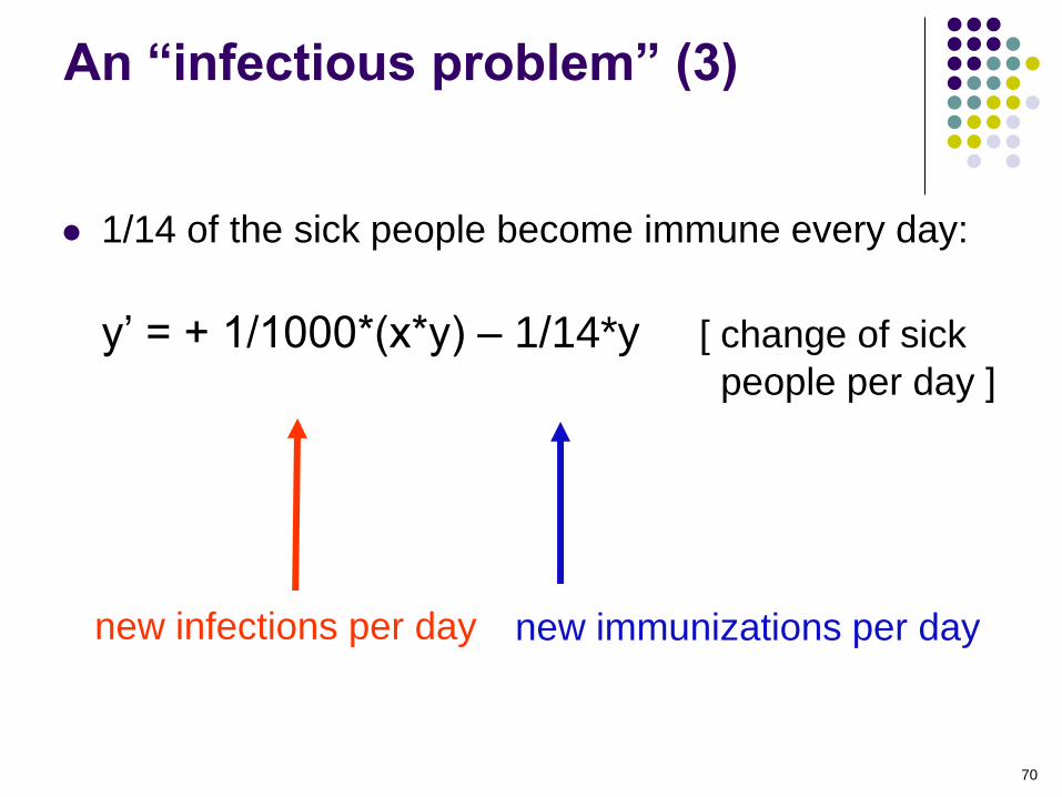
An “infectious problem” (3)
1/14 of the sick people become immune every day:
y’ = + 1/1000*(x*y) – 1/14*y [ change of sick
people per day ]
new infections per day new immunizations per day

71
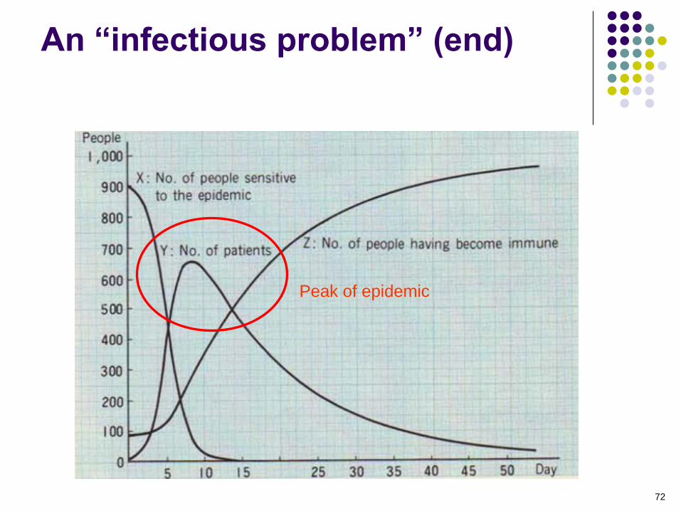
An “infectious problem” (4)
z’ = 1/14 *y [ change of people having
recovered per day,
now immune ]
Model:
x’ = - 1/1000*(x*y) change not yet infected/day
y’ = + 1/1000*(x*y) – 1/14*y change of sick/day
z’ = 1/14 *y change of immunized/day
72
An “infectious problem” (end)
Peak of epidemic
73
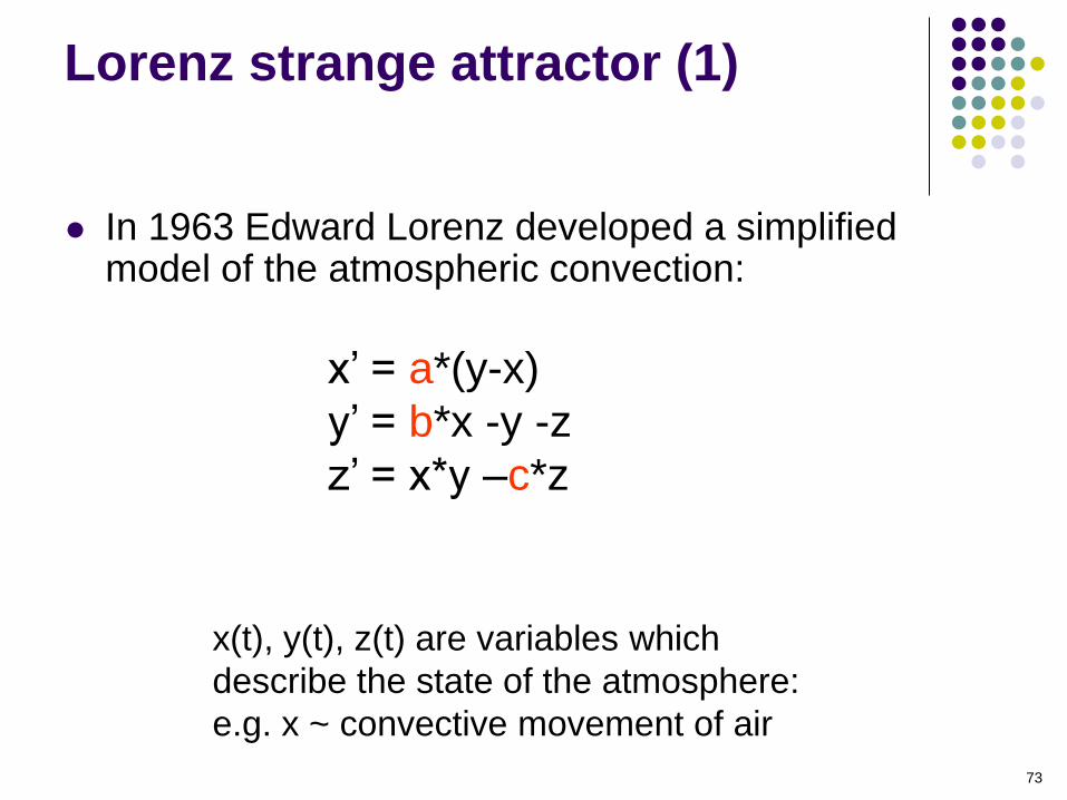
Lorenz strange attractor (1)
In 1963 Edward Lorenz developed a simplified model of the atmospheric convection:
x(t), y(t), z(t) are variables which
describe the state of the atmosphere:
e.g. x ~ convective movement of air
x’ = a*(y-x)
y’ = b*x -y -z
z’ = x*y –c*z
74
Lorenz strange attractor (2)
Lorenz found that for the particular values
a = 10, b = 8/3 and c =28
the solutions x(t), y(t), z(t) become chaotic when
the variable time (t) cycles through a range of
values.
This was the start of the “chaos theory” and its
related theory of fractals.
75
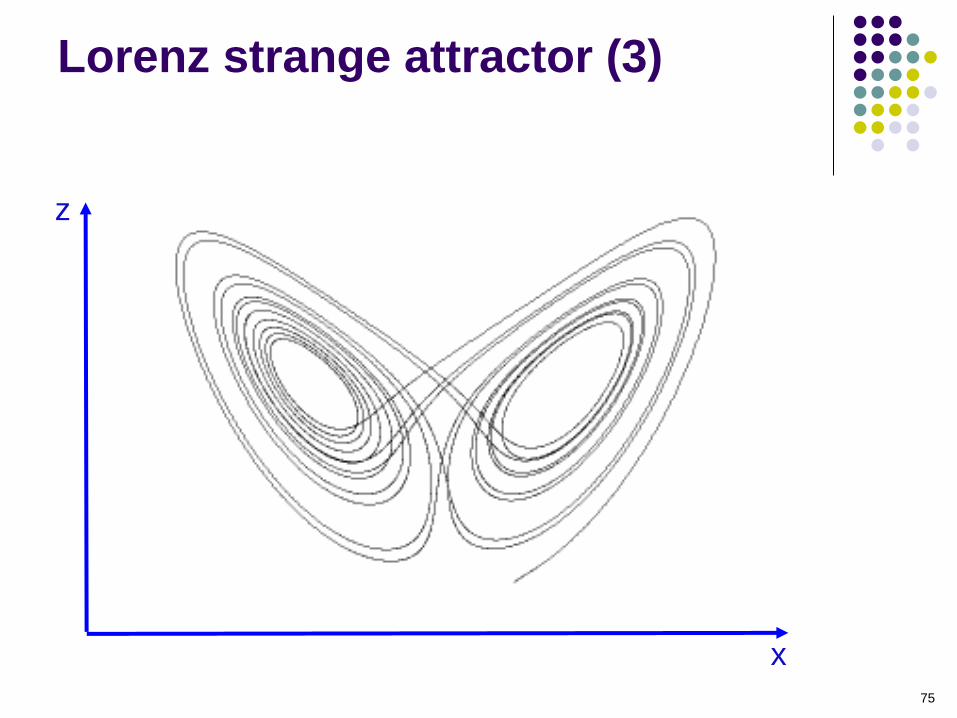
Lorenz strange attractor (3)
x
z
76
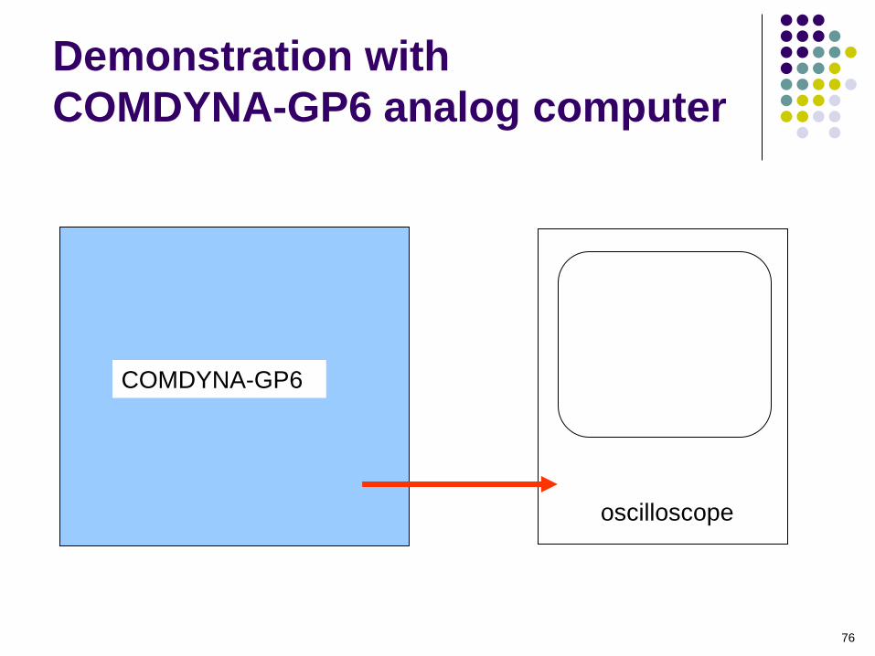
Demonstration with
COMDYNA-GP6 analog computer
COMDYNA-GP6
oscilloscope
77
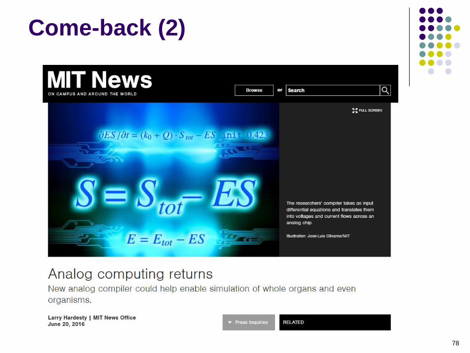
A possible come-back of the
analog computer ? (1)
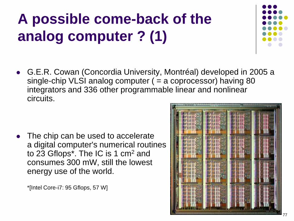
G.E.R. Cowan (Concordia University, Montréal) developed in 2005 a single-chip VLSI analog computer ( = a coprocessor) having 80 integrators and 336 other programmable linear and nonlinear circuits.
The chip can be used to accelerate a digital computer's numerical routines to 23 Gflops*. The IC is 1 cm2 and consumes 300 mW, still the lowest energy use of the world. *[Intel Core-i7: 95 Gflops, 57 W]
78
Come-back (2)
79
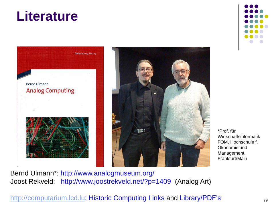
Literature
Bernd Ulmann*: http://www.analogmuseum.org/
Joost Rekveld: http://www.joostrekveld.net/?p=1409 (Analog Art)
http://computarium.lcd.lu: Historic Computing Links and Library/PDF’s
*Prof. für
Wirtschaftsinformatik
FOM, Hochschule f.
Ökonomie und
Management,
Frankfurt/Main

80
Merci fir d’Nolauschteren!
Slides sinn op
http://computarium.lcd.lu/news.html