Embed Size (px)
Citation preview
arX
iv:1
407.
1296
v1 [
mat
h.O
C]
4 J
ul 2
014
An Accelerated Proximal Coordinate Gradient Method and its
Application to Regularized Empirical Risk Minimization
Qihang Lin∗ Zhaosong Lu† Lin Xiao‡
July 7, 2014
Abstract
We consider the problem of minimizing the sum of two convex functions: one is smooth andgiven by a gradient oracle, and the other is separable over blocks of coordinates and has a simpleknown structure over each block. We develop an accelerated randomized proximal coordinategradient (APCG) method for minimizing such convex composite functions. For strongly convexfunctions, our method achieves faster linear convergence rates than existing randomized prox-imal coordinate gradient methods. Without strong convexity, our method enjoys acceleratedsublinear convergence rates. We show how to apply the APCG method to solve the regularizedempirical risk minimization (ERM) problem, and devise efficient implementations that avoidfull-dimensional vector operations. For ill-conditioned ERM problems, our method obtains im-proved convergence rates than the state-of-the-art stochastic dual coordinate ascent (SDCA)method.
1 Introduction
Coordinate descent methods have received extensive attention in recent years due to its potentialfor solving large-scale optimization problems arising from machine learning and other applications(e.g., [29, 10, 47, 17, 45, 30]). In this paper, we develop an accelerated proximal coordinate gradient(APCG) method for solving problems of the following form:
minimizex∈RN
{F (x)
def= f(x) + Ψ(x)
}, (1)
where f and Ψ are proper and lower semicontinuous convex functions [34, Section 7]. Moreover,we assume that f is differentiable on R
N , and Ψ has a block separable structure, i.e.,
Ψ(x) =
n∑
i=1
Ψi(xi), (2)
where each xi denotes a sub-vector of x with cardinality Ni, and the collection {xi : i = 1, . . . , n}form a partition of the components of x. In addition to the capability of modeling nonsmooth
∗Tippie College of Business, The University of Iowa, Iowa City, IA 52242, USA. Email: [email protected].†Department of Mathematics, Simon Fraser University, Surrey, BC V3T 0A3, Canada. Email: [email protected].‡Machine Learning Groups, Microsoft Research, Redmond, WA 98052, USA. Email: [email protected].
1
terms such as Ψ(x) = λ‖x‖1, this model also includes optimization problems with block separableconstraints. More specifically, each block constraints xi ∈ Ci, where Ci is a closed convex set, canbe modeled by an indicator function defined as Ψi(xi) = 0 if xi ∈ Ci and ∞ otherwise.
At each iteration, coordinate descent methods choose one block of coordinates xi to sufficientlyreduce the objective value while keeping other blocks fixed. In order to exploit the known structureof each Ψi, a proximal coordinate gradient step can be taken [33]. To be more specific, given thecurrent iterate x(k), we pick a block ik ∈ {1, . . . , n} and solve a block-wise proximal subproblem inthe form of
h(k)ik
= argminh∈ℜNik
{
〈∇ikf(x(k)), h〉 + Lik
2‖h‖2 +Ψik(x
(k)ik
+ h)
}
, (3)
and then set the next iterate as
x(k+1)i =
{
x(k)ik
+ h(k)ik
, if i = ik,
x(k)i , if i 6= ik,
i = 1, . . . , n. (4)
Here ∇if(x) denotes the partial gradient of f with respect to xi, and Li is the Lipschitz constantof the partial gradient (which will be defined precisely later).
One common approach for choosing such a block is the cyclic scheme. The global and localconvergence properties of the cyclic coordinate descent method have been studied in, e.g., [41, 22,36, 2, 9]. Recently, randomized strategies for choosing the block to update became more popular[38, 15, 26, 33]. In addition to its theoretical benefits (randomized schemes are in general easierto analyze than the cyclic scheme), numerous experiments have demonstrated that randomizedcoordinate descent methods are very powerful for solving large-scale machine learning problems [6,10, 38, 40]. Their efficiency can be further improved with parallel and distributed implementations[5, 31, 32, 23, 19]. Randomized block coordinate descent methods have also been proposed andanalyzed for solving problems with coupled linear constraints [43, 24] and a class of structurednonconvex optimization problems (e.g., [21, 28]). Coordinate descent methods with more generalschemes of choosing the block to update have also been studied; see, e.g., [3, 44, 46].
Inspired by the success of accelerated full gradient methods [25, 1, 42, 27], several recent workextended Nesterov’s acceleration technique to speed up randomized coordinate descent methods.In particular, Nesterov [26] developed an accelerated randomized coordinate gradient method forminimizing unconstrained smooth functions, which corresponds to the case of Ψ(x) ≡ 0 in (1).Lu and Xiao [20] gave a sharper convergence analysis of Nesterov’s method using a randomizedestimate sequence framework, and Lee and Sidford [14] developed extensions using weighted randomsampling schemes. Accelerated coordinate gradient methods have also been used to speed up thesolution of linear systems [14, 18]. More recently, Fercoq and Richtarik [8] proposed an APPROX(Accelerated, Parallel and PROXimal) coordinate descent method for solving the more generalproblem (1) and obtained accelerated sublinear convergence rate, but their method cannot exploitthe strong convexity of the objective function to obtain accelerated linear rates.
In this paper, we propose a general APCG method that achieves accelerated linear convergencerates when the objective function is strongly convex. Without the strong convexity assumption,our method recovers a special case of the APPROX method [8]. Moreover, we show how to applythe APCG method to solve the regularized empirical risk minimization (ERM) problem, and deviseefficient implementations that avoid full-dimensional vector operations. For ill-conditioned ERMproblems, our method obtains improved convergence rates than the state-of-the-art stochastic dualcoordinate ascent (SDCA) method [40].
2
1.1 Outline of paper
This paper is organized as follows. The rest of this section introduces some notations and stateour main assumptions. In Section 2, we present the general APCG method and our main theoremon its convergence rate. We also give two simplified versions of APCG depending on whether ornot the function f is strongly convex, and explain how to exploit strong convexity in Ψ. Section 3is devoted to the convergence analysis that proves our main theorem. In Section 4, we deriveequivalent implementations of the APCG method that can avoid full-dimensional vector operations.
In Section 5, we apply the APCG method to solve the dual of the regularized ERM problemand give the corresponding complexity results. We also explain how to recover primal solutions toguarantee the same rate of convergence for the primal-dual gap. In addition, we present numericalexperiments to demonstrate the performance of the APCG method.
1.2 Notations and assumptions
For any partition of x ∈ RN into {xi ∈ R
Ni : i = 1, . . . , n} with∑n
i=1Ni = N , there is an N ×Npermutation matrix U partitioned as U = [U1 · · ·Un], where Ui ∈ R
N×Ni , such that
x =
n∑
i=1
Uixi, and xi = UTi x, i = 1, . . . , n.
For any x ∈ RN , the partial gradient of f with respect to xi is defined as
∇if(x) = UTi ∇f(x), i = 1, . . . , n.
We associate each subspace RNi , for i = 1, . . . , n, with the standard Euclidean norm, denoted ‖·‖2.We make the following assumptions which are standard in the literature on coordinate descentmethods (e.g., [26, 33]).
Assumption 1. The gradient of function f is block-wise Lipschitz continuous with constants Li,i.e.,
‖∇if(x+ Uihi)−∇if(x)‖2 ≤ Li‖hi‖2, ∀hi ∈ RNi , i = 1, . . . , n, x ∈ R
N .
An immediate consequence of Assumption 1 is (see, e.g., [25, Lemma 1.2.3])
f(x+ Uihi) ≤ f(x) + 〈∇if(x), hi〉+Li
2‖hi‖22, ∀hi ∈ R
Ni , i = 1, . . . , n, x ∈ RN . (5)
For convenience, we define the following weighted norm in the whole space RN :
‖x‖L =
( n∑
i=1
Li‖xi‖22)1/2
, ∀x ∈ RN . (6)
Assumption 2. There exists µ ≥ 0 such that for all y ∈ RN and x ∈ dom (Ψ),
f(y) ≥ f(x) + 〈∇f(x), y − x〉+ µ
2‖y − x‖2L.
The convexity parameter of f with respect to the norm ‖ · ‖L is the largest µ such that theabove inequality holds. Every convex function satisfies Assumption 2 with µ = 0. If µ > 0, thenthe function f is called strongly convex.
Remark. Together with (5) and the definition of ‖ · ‖L in (6), Assumption 2 implies µ ≤ 1.
3
Algorithm 1 The APCG method
input: x(0) ∈ dom (Ψ) and convexity parameter µ ≥ 0.
initialize: set z(0) = x(0) and choose 0 < γ0 ∈ [µ, 1].
iterate: repeat for k = 0, 1, 2, . . .
1. Compute αk ∈ (0, 1n ] from the equation
n2α2k = (1− αk) γk + αkµ, (7)
and setγk+1 = (1− αk)γk + αkµ, βk =
αkµ
γk+1. (8)
2. Compute y(k) as
y(k) =1
αkγk + γk+1
(
αkγkz(k) + γk+1x
(k))
. (9)
3. Choose ik ∈ {1, . . . , n} uniformly at random and compute
z(k+1) = argminx∈RN
{nαk
2
∥∥x− (1− βk)z
(k) − βky(k)∥∥2
L+ 〈∇ikf(y
(k)), xik〉+Ψik(xik)}
.
4. Setx(k+1) = y(k) + nαk(z
(k+1) − z(k)) +µ
n(z(k) − y(k)). (10)
2 The APCG method
In this section we describe the general APCG method, and its two simplified versions under differentassumptions (whether or not the objective function is strong convex). We also present our maintheorem on the convergence rates of the APCG method.
We first explain the notations used in our algorithms. The algorithms proceed in iterations,with k being the iteration counter. Lower case letters x, y, z represent vectors in the full space RN ,and x(k), y(k) and z(k) are their values at the kth iteration. Each block coordinate is indicated with
a subscript, for example, x(k)i represent the value of the ith block of the vector x(k). The Greek
letters α, β, γ are scalars, and αk, βk and γk represent their values at iteration k. For scalars, asuperscript represents the power exponent; for example, n2, α2
k denotes the squares of n and αk
respectively.The general APCG method is given as Algorithm 1. At each iteration k, the APCG method
picks a random coordinate ik ∈ {1, . . . , n} and generates y(k), x(k+1) and z(k+1). One can observethat x(k+1) and z(k+1) depend on the realization of the random variable
ξk = {i0, i1, . . . , ik},
while y(k) is independent of ik and only depends on ξk−1.To better understand this method, we make the following observations. For convenience, we
4
define
z(k+1) = argminx∈RN
{nαk
2
∥∥x− (1− βk)z
(k) − βky(k)∥∥2
L+ 〈∇f(y(k)), x− y(k)〉+Ψ(x)
}
, (11)
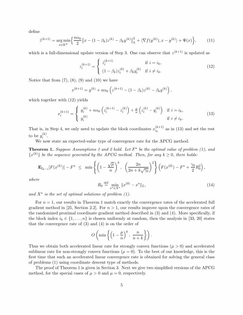
which is a full-dimensional update version of Step 3. One can observe that z(k+1) is updated as
z(k+1)i =
z(k+1)i if i = ik,
(1− βk)z(k)i + βky
(k)i if i 6= ik.
(12)
Notice that from (7), (8), (9) and (10) we have
x(k+1) = y(k) + nαk
(
z(k+1) − (1− βk)z(k) − βky
(k))
,
which together with (12) yields
x(k+1)i =
y(k)i + nαk
(
z(k+1)i − z
(k)i
)
+ µn
(
z(k)i − y
(k)i
)
if i = ik,
y(k)i if i 6= ik.
(13)
That is, in Step 4, we only need to update the block coordinates x(k+1)ik
as in (13) and set the rest
to be y(k)i .
We now state an expected-value type of convergence rate for the APCG method.
Theorem 1. Suppose Assumptions 1 and 2 hold. Let F ⋆ be the optimal value of problem (1), and{x(k)} be the sequence generated by the APCG method. Then, for any k ≥ 0, there holds:
Eξk−1[F (x(k))]− F ⋆ ≤ min
{(
1−√µ
n
)k
,
(2n
2n+ k√γ0
)2}(
F (x(0))− F ⋆ +γ02R2
0
)
,
whereR0
def= min
x⋆∈X⋆‖x(0) − x⋆‖L, (14)
and X⋆ is the set of optimal solutions of problem (1).
For n = 1, our results in Theorem 1 match exactly the convergence rates of the accelerated fullgradient method in [25, Section 2.2]. For n > 1, our results improve upon the convergence rates ofthe randomized proximal coordinate gradient method described in (3) and (4). More specifically, ifthe block index ik ∈ {1, . . . , n} is chosen uniformly at random, then the analysis in [33, 20] statesthat the convergence rate of (3) and (4) is on the order of
O
(
min
{(
1− µ
n
)k,
n
n+ k
})
.
Thus we obtain both accelerated linear rate for strongly convex functions (µ > 0) and acceleratedsublinear rate for non-strongly convex functions (µ = 0). To the best of our knowledge, this is thefirst time that such an accelerated linear convergence rate is obtained for solving the general classof problems (1) using coordinate descent type of methods.
The proof of Theorem 1 is given in Section 3. Next we give two simplified versions of the APCGmethod, for the special cases of µ > 0 and µ = 0, respectively.
5
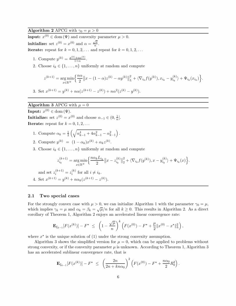
Algorithm 2 APCG with γ0 = µ > 0
input: x(0) ∈ dom (Ψ) and convexity parameter µ > 0.
initialize: set z(0) = x(0) and α =√µn .
iterate: repeat for k = 0, 1, 2, . . . and repeat for k = 0, 1, 2, . . .
1. Compute y(k) = x(k)+αz(k)
1+α .
2. Choose ik ∈ {1, . . . , n} uniformly at random and compute
z(k+1) = argminx∈RN
{nα
2
∥∥x− (1− α)z(k) − αy(k)
∥∥2
L+ 〈∇ikf(y
(k)), xik − y(k)ik
〉+Ψik(xik)}
.
3. Set x(k+1) = y(k) + nα(z(k+1) − z(k)) + nα2(z(k) − y(k)).
Algorithm 3 APCG with µ = 0
Input: x(0) ∈ dom (Ψ).
Initialize: set z(0) = x(0) and choose α−1 ∈ (0, 1n ].
Iterate: repeat for k = 0, 1, 2, . . .
1. Compute αk = 12
(√
α4k−1 + 4α2
k−1 − α2k−1
)
.
2. Compute y(k) = (1− αk)x(k) + αkz
(k).
3. Choose ik ∈ {1, . . . , n} uniformly at random and compute
z(k+1)ik
= argminx∈RN
{nαkLik
2
∥∥x− z
(k)ik
∥∥2
2+ 〈∇ikf(y
(k)), x− y(k)ik
〉+Ψik(x)}
.
and set z(k+1)i = z
(k)i for all i 6= ik.
4. Set x(k+1) = y(k) + nαk(z(k+1) − z(k)).
2.1 Two special cases
For the strongly convex case with µ > 0, we can initialize Algorithm 1 with the parameter γ0 = µ,which implies γk = µ and αk = βk =
√µ/n for all k ≥ 0. This results in Algorithm 2. As a direct
corollary of Theorem 1, Algorithm 2 enjoys an accelerated linear convergence rate:
Eξk−1[F (x(k))]− F ⋆ ≤
(
1−√µ
n
)k (
F (x(0))− F ⋆ +µ
2‖x(0) − x⋆‖2L
)
,
where x⋆ is the unique solution of (1) under the strong convexity assumption.Algorithm 3 shows the simplified version for µ = 0, which can be applied to problems without
strong convexity, or if the convexity parameter µ is unknown. According to Theorem 1, Algorithm 3has an accelerated sublinear convergence rate, that is
Eξk−1[F (x(k))]− F ⋆ ≤
(2n
2n+ knα0
)2 (
F (x(0))− F ⋆ +nα0
2R2
0
)
.
6
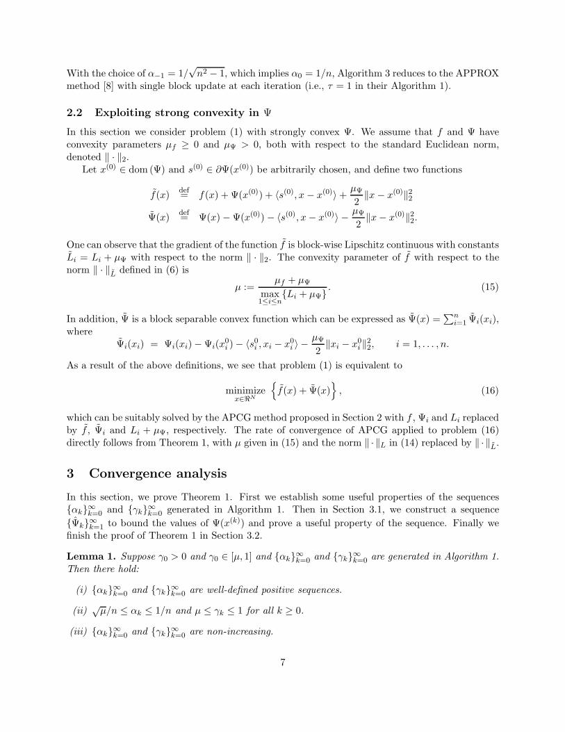
With the choice of α−1 = 1/√n2 − 1, which implies α0 = 1/n, Algorithm 3 reduces to the APPROX
method [8] with single block update at each iteration (i.e., τ = 1 in their Algorithm 1).
2.2 Exploiting strong convexity in Ψ
In this section we consider problem (1) with strongly convex Ψ. We assume that f and Ψ haveconvexity parameters µf ≥ 0 and µΨ > 0, both with respect to the standard Euclidean norm,denoted ‖ · ‖2.
Let x(0) ∈ dom (Ψ) and s(0) ∈ ∂Ψ(x(0)) be arbitrarily chosen, and define two functions
f(x)def= f(x) + Ψ(x(0)) + 〈s(0), x− x(0)〉+ µΨ
2‖x− x(0)‖22
Ψ(x)def= Ψ(x)−Ψ(x(0))− 〈s(0), x− x(0)〉 − µΨ
2‖x− x(0)‖22.
One can observe that the gradient of the function f is block-wise Lipschitz continuous with constantsLi = Li + µΨ with respect to the norm ‖ · ‖2. The convexity parameter of f with respect to thenorm ‖ · ‖L defined in (6) is
µ :=µf + µΨ
max1≤i≤n
{Li + µΨ}. (15)
In addition, Ψ is a block separable convex function which can be expressed as Ψ(x) =∑n
i=1 Ψi(xi),where
Ψi(xi) = Ψi(xi)−Ψi(x0i )− 〈s0i , xi − x0i 〉 −
µΨ
2‖xi − x0i ‖22, i = 1, . . . , n.
As a result of the above definitions, we see that problem (1) is equivalent to
minimizex∈ℜN
{
f(x) + Ψ(x)}
, (16)
which can be suitably solved by the APCG method proposed in Section 2 with f , Ψi and Li replacedby f , Ψi and Li + µΨ, respectively. The rate of convergence of APCG applied to problem (16)directly follows from Theorem 1, with µ given in (15) and the norm ‖ · ‖L in (14) replaced by ‖ · ‖L.
3 Convergence analysis
In this section, we prove Theorem 1. First we establish some useful properties of the sequences{αk}∞k=0 and {γk}∞k=0 generated in Algorithm 1. Then in Section 3.1, we construct a sequence
{Ψk}∞k=1 to bound the values of Ψ(x(k)) and prove a useful property of the sequence. Finally wefinish the proof of Theorem 1 in Section 3.2.
Lemma 1. Suppose γ0 > 0 and γ0 ∈ [µ, 1] and {αk}∞k=0 and {γk}∞k=0 are generated in Algorithm 1.Then there hold:
(i) {αk}∞k=0 and {γk}∞k=0 are well-defined positive sequences.
(ii)√µ/n ≤ αk ≤ 1/n and µ ≤ γk ≤ 1 for all k ≥ 0.
(iii) {αk}∞k=0 and {γk}∞k=0 are non-increasing.
7
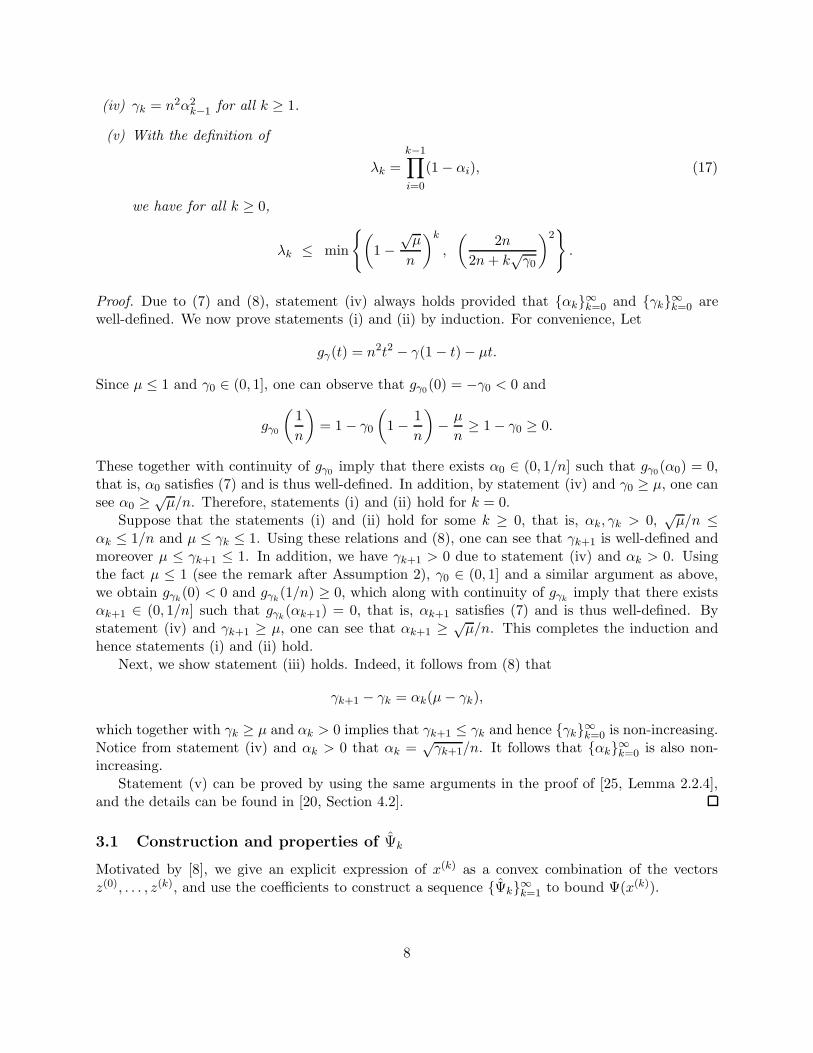
(iv) γk = n2α2k−1 for all k ≥ 1.
(v) With the definition of
λk =
k−1∏
i=0
(1− αi), (17)
we have for all k ≥ 0,
λk ≤ min
{(
1−√µ
n
)k
,
(2n
2n+ k√γ0
)2}
.
Proof. Due to (7) and (8), statement (iv) always holds provided that {αk}∞k=0 and {γk}∞k=0 arewell-defined. We now prove statements (i) and (ii) by induction. For convenience, Let
gγ(t) = n2t2 − γ(1− t)− µt.
Since µ ≤ 1 and γ0 ∈ (0, 1], one can observe that gγ0(0) = −γ0 < 0 and
gγ0
(1
n
)
= 1− γ0
(
1− 1
n
)
− µ
n≥ 1− γ0 ≥ 0.
These together with continuity of gγ0 imply that there exists α0 ∈ (0, 1/n] such that gγ0(α0) = 0,that is, α0 satisfies (7) and is thus well-defined. In addition, by statement (iv) and γ0 ≥ µ, one cansee α0 ≥
õ/n. Therefore, statements (i) and (ii) hold for k = 0.
Suppose that the statements (i) and (ii) hold for some k ≥ 0, that is, αk, γk > 0,√µ/n ≤
αk ≤ 1/n and µ ≤ γk ≤ 1. Using these relations and (8), one can see that γk+1 is well-defined andmoreover µ ≤ γk+1 ≤ 1. In addition, we have γk+1 > 0 due to statement (iv) and αk > 0. Usingthe fact µ ≤ 1 (see the remark after Assumption 2), γ0 ∈ (0, 1] and a similar argument as above,we obtain gγk(0) < 0 and gγk(1/n) ≥ 0, which along with continuity of gγk imply that there existsαk+1 ∈ (0, 1/n] such that gγk(αk+1) = 0, that is, αk+1 satisfies (7) and is thus well-defined. Bystatement (iv) and γk+1 ≥ µ, one can see that αk+1 ≥ √
µ/n. This completes the induction andhence statements (i) and (ii) hold.
Next, we show statement (iii) holds. Indeed, it follows from (8) that
γk+1 − γk = αk(µ− γk),
which together with γk ≥ µ and αk > 0 implies that γk+1 ≤ γk and hence {γk}∞k=0 is non-increasing.Notice from statement (iv) and αk > 0 that αk =
√γk+1/n. It follows that {αk}∞k=0 is also non-
increasing.Statement (v) can be proved by using the same arguments in the proof of [25, Lemma 2.2.4],
and the details can be found in [20, Section 4.2].
3.1 Construction and properties of Ψk
Motivated by [8], we give an explicit expression of x(k) as a convex combination of the vectorsz(0), . . . , z(k), and use the coefficients to construct a sequence {Ψk}∞k=1 to bound Ψ(x(k)).
8
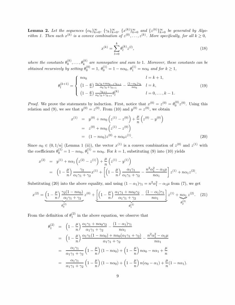
Lemma 2. Let the sequences {αk}∞k=0, {γk}∞k=0, {x(k)}∞k=0 and {z(k)}∞k=0 be generated by Algo-rithm 1. Then each x(k) is a convex combination of z(0), . . . , z(k). More specifically, for all k ≥ 0,
x(k) =k∑
l=0
θ(k)l z(l), (18)
where the constants θ(k)0 , . . . , θ
(k)k are nonnegative and sum to 1. Moreover, these constants can be
obtained recursively by setting θ(0)0 = 1, θ
(1)0 = 1− nα0, θ
(1)1 = nα0 and for k ≥ 1,
θ(k+1)l =
nαk l = k + 1,(1− µ
n
) αkγk+nαk−1γk+1
αkγk+γk+1− (1−αk)γk
nαkl = k,
(1− µ
n
) γk+1
αkγk+γk+1θ(k)l l = 0, . . . , k − 1.
(19)
Proof. We prove the statements by induction. First, notice that x(0) = z(0) = θ(0)0 z(0). Using this
relation and (9), we see that y(0) = z(0). From (10) and y(0) = z(0), we obtain
x(1) = y(0) + nα0
(
z(1) − z(0))
+µ
n
(
z(0) − y(0))
= z(0) + nα0
(
z(1) − z(0))
= (1 − nα0)z(0) + nα0z
(1). (20)
Since α0 ∈ (0, 1/n] (Lemma 1 (ii)), the vector x(1) is a convex combination of z(0) and z(1) with
the coefficients θ(1)0 = 1− nα0, θ
(1)1 = nα0. For k = 1, substituting (9) into (10) yields
x(2) = y(1) + nα1
(
z(2) − z(1))
+µ
n
(
z(1) − y(1))
=(
1− µ
n
) γ2α1γ1 + γ2
x(1) +
[(
1− µ
n
) α1γ1α1γ1 + γ2
− n2α21 − α1µ
nα1
]
z(1) + nα1z(2).
Substituting (20) into the above equality, and using (1− α1)γ1 = n2α21 − α1µ from (7), we get
x(2) =(
1− µ
n
) γ2(1− nα0)
α1γ1 + γ2︸ ︷︷ ︸
θ(2)0
z(0) +
[(
1− µ
n
) α1γ1 + nα0γ2α1γ1 + γ2
− (1− α1)γ1nα1
]
︸ ︷︷ ︸
θ(2)1
z(1) + nα1︸︷︷︸
θ(2)2
z(2). (21)
From the definition of θ(2)1 in the above equation, we observe that
θ(2)1 =
(
1− µ
n
) α1γ1 + nα0γ2α1γ1 + γ2
− (1− α1)γ1nα1
=(
1− µ
n
) α1γ1(1− nα0) + nα0(α1γ1 + γ2)
α1γ1 + γ2− n2α2
1 − α1µ
nα1
=α1γ1
α1γ1 + γ2
(
1− µ
n
)
(1− nα0) +(
1− µ
n
)
nα0 − nα1 +µ
n
=α1γ1
α1γ1 + γ2
(
1− µ
n
)
(1− nα0) +(
1− µ
n
)
n(α0 − α1) +µ
n(1− nα1).
9
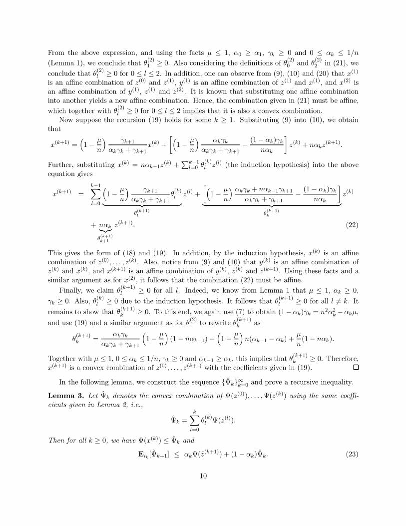
From the above expression, and using the facts µ ≤ 1, α0 ≥ α1, γk ≥ 0 and 0 ≤ αk ≤ 1/n
(Lemma 1), we conclude that θ(2)1 ≥ 0. Also considering the definitions of θ
(2)0 and θ
(2)2 in (21), we
conclude that θ(2)l ≥ 0 for 0 ≤ l ≤ 2. In addition, one can observe from (9), (10) and (20) that x(1)
is an affine combination of z(0) and z(1), y(1) is an affine combination of z(1) and x(1), and x(2) isan affine combination of y(1), z(1) and z(2). It is known that substituting one affine combinationinto another yields a new affine combination. Hence, the combination given in (21) must be affine,
which together with θ(2)l ≥ 0 for 0 ≤ l ≤ 2 implies that it is also a convex combination.
Now suppose the recursion (19) holds for some k ≥ 1. Substituting (9) into (10), we obtainthat
x(k+1) =(
1− µ
n
) γk+1
αkγk + γk+1x(k) +
[(
1− µ
n
) αkγkαkγk + γk+1
− (1− αk)γknαk
]
z(k) + nαkz(k+1).
Further, substituting x(k) = nαk−1z(k) +
∑k−1l=0 θ
(k)l z(l) (the induction hypothesis) into the above
equation gives
x(k+1) =
k−1∑
l=0
(
1− µ
n
) γk+1
αkγk + γk+1θ(k)l
︸ ︷︷ ︸
θ(k+1)l
z(l) +
[(
1− µ
n
) αkγk + nαk−1γk+1
αkγk + γk+1− (1− αk)γk
nαk
]
︸ ︷︷ ︸
θ(k+1)k
z(k)
+ nαk︸︷︷︸
θ(k+1)k+1
z(k+1). (22)
This gives the form of (18) and (19). In addition, by the induction hypothesis, x(k) is an affinecombination of z(0), . . . , z(k). Also, notice from (9) and (10) that y(k) is an affine combination ofz(k) and x(k), and x(k+1) is an affine combination of y(k), z(k) and z(k+1). Using these facts and asimilar argument as for x(2), it follows that the combination (22) must be affine.
Finally, we claim θ(k+1)l ≥ 0 for all l. Indeed, we know from Lemma 1 that µ ≤ 1, αk ≥ 0,
γk ≥ 0. Also, θ(k)l ≥ 0 due to the induction hypothesis. It follows that θ
(k+1)l ≥ 0 for all l 6= k. It
remains to show that θ(k+1)k ≥ 0. To this end, we again use (7) to obtain (1−αk)γk = n2α2
k −αkµ,
and use (19) and a similar argument as for θ(2)1 to rewrite θ
(k+1)k as
θ(k+1)k =
αkγkαkγk + γk+1
(
1− µ
n
)
(1− nαk−1) +(
1− µ
n
)
n(αk−1 − αk) +µ
n(1− nαk).
Together with µ ≤ 1, 0 ≤ αk ≤ 1/n, γk ≥ 0 and αk−1 ≥ αk, this implies that θ(k+1)k ≥ 0. Therefore,
x(k+1) is a convex combination of z(0), . . . , z(k+1) with the coefficients given in (19).
In the following lemma, we construct the sequence {Ψk}∞k=0 and prove a recursive inequality.
Lemma 3. Let Ψk denotes the convex combination of Ψ(z(0)), . . . ,Ψ(z(k)) using the same coeffi-cients given in Lemma 2, i.e.,
Ψk =
k∑
l=0
θ(k)l Ψ(z(l)).
Then for all k ≥ 0, we have Ψ(x(k)) ≤ Ψk and
Eik [Ψk+1] ≤ αkΨ(z(k+1)) + (1− αk)Ψk. (23)
10
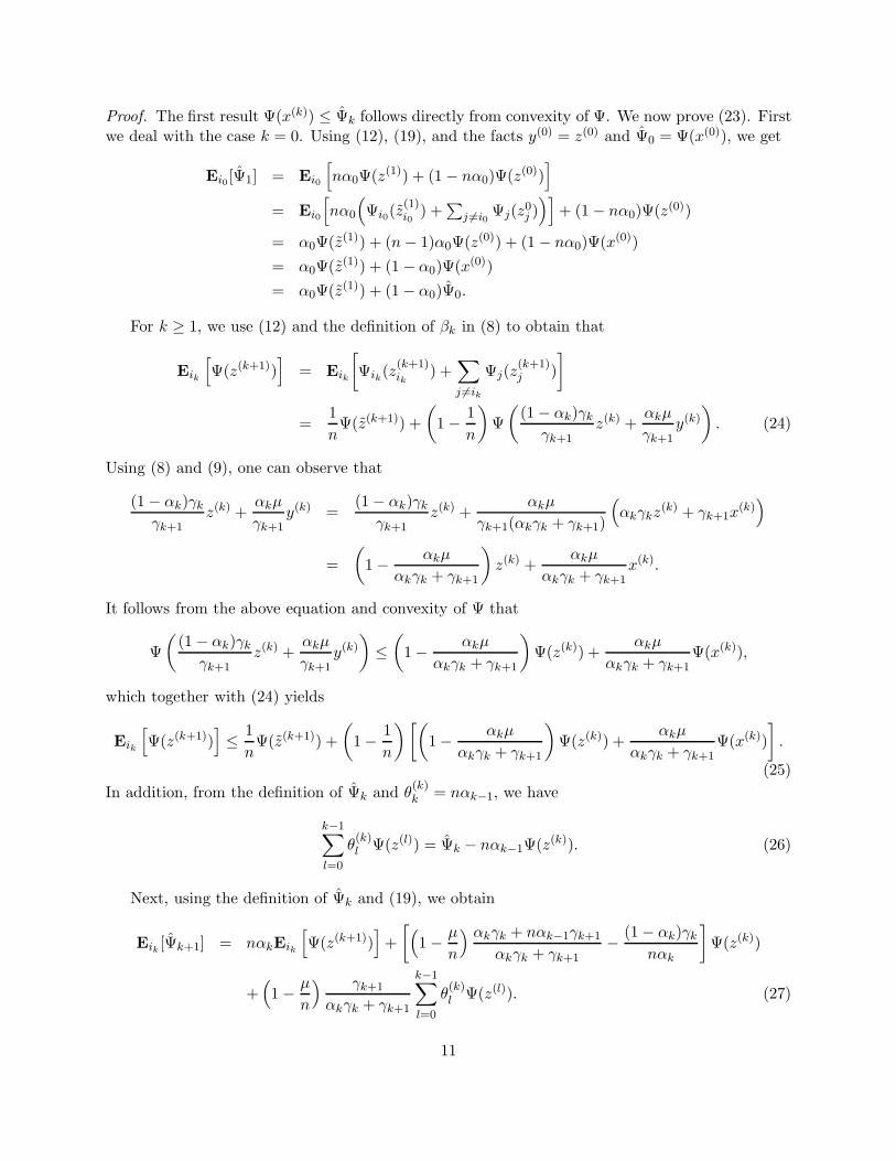
Proof. The first result Ψ(x(k)) ≤ Ψk follows directly from convexity of Ψ. We now prove (23). Firstwe deal with the case k = 0. Using (12), (19), and the facts y(0) = z(0) and Ψ0 = Ψ(x(0)), we get
Ei0 [Ψ1] = Ei0
[
nα0Ψ(z(1)) + (1− nα0)Ψ(z(0))]
= Ei0
[
nα0
(
Ψi0(z(1)i0
) +∑
j 6=i0Ψj(z
0j ))]
+ (1− nα0)Ψ(z(0))
= α0Ψ(z(1)) + (n− 1)α0Ψ(z(0)) + (1− nα0)Ψ(x(0))
= α0Ψ(z(1)) + (1− α0)Ψ(x(0))
= α0Ψ(z(1)) + (1− α0)Ψ0.
For k ≥ 1, we use (12) and the definition of βk in (8) to obtain that
Eik
[
Ψ(z(k+1))]
= Eik
[
Ψik(z(k+1)ik
) +∑
j 6=ik
Ψj(z(k+1)j )
]
=1
nΨ(z(k+1)) +
(
1− 1
n
)
Ψ
((1− αk)γk
γk+1z(k) +
αkµ
γk+1y(k)
)
. (24)
Using (8) and (9), one can observe that
(1− αk)γkγk+1
z(k) +αkµ
γk+1y(k) =
(1− αk)γkγk+1
z(k) +αkµ
γk+1(αkγk + γk+1)
(
αkγkz(k) + γk+1x
(k))
=
(
1− αkµ
αkγk + γk+1
)
z(k) +αkµ
αkγk + γk+1x(k).
It follows from the above equation and convexity of Ψ that
Ψ
((1− αk)γk
γk+1z(k) +
αkµ
γk+1y(k)
)
≤(
1− αkµ
αkγk + γk+1
)
Ψ(z(k)) +αkµ
αkγk + γk+1Ψ(x(k)),
which together with (24) yields
Eik
[
Ψ(z(k+1))]
≤ 1
nΨ(z(k+1)) +
(
1− 1
n
)[(
1− αkµ
αkγk + γk+1
)
Ψ(z(k)) +αkµ
αkγk + γk+1Ψ(x(k))
]
.
(25)
In addition, from the definition of Ψk and θ(k)k = nαk−1, we have
k−1∑
l=0
θ(k)l Ψ(z(l)) = Ψk − nαk−1Ψ(z(k)). (26)
Next, using the definition of Ψk and (19), we obtain
Eik [Ψk+1] = nαkEik
[
Ψ(z(k+1))]
+
[(
1− µ
n
) αkγk + nαk−1γk+1
αkγk + γk+1− (1− αk)γk
nαk
]
Ψ(z(k))
+(
1− µ
n
) γk+1
αkγk + γk+1
k−1∑
l=0
θ(k)l Ψ(z(l)). (27)
11
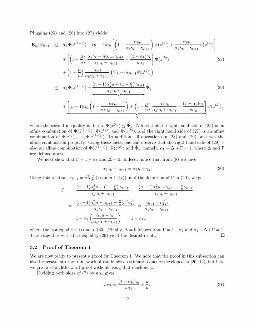
Plugging (25) and (26) into (27) yields
Eik [Ψk+1] ≤ αkΨ(z(k+1)) + (n − 1)αk
[(
1− αkµ
αkγk + γk+1
)
Ψ(z(k)) +αkµ
αkγk + γk+1Ψ(x(k))
]
+
[(
1− µ
n
) αkγk + nαk−1γk+1
αkγk + γk+1− (1− αk)γk
nαk
]
Ψ(z(k)) (28)
+(
1− µ
n
) γk+1
αkγk + γk+1
(
Ψk − nαk−1Ψ(z(k)))
≤ αkΨ(z(k+1)) +(n − 1)α2
kµ+(1− µ
n
)γk+1
αkγk + γk+1︸ ︷︷ ︸
Γ
Ψk (29)
+
[
(n− 1)αk
(
1− αkµ
αkγk + γk+1
)
+(
1− µ
n
) αkγkαkγk + γk+1
− (1− αk)γknαk
]
︸ ︷︷ ︸
∆
Ψ(z(k)),
where the second inequality is due to Ψ(x(k)) ≤ Ψk. Notice that the right hand side of (25) is anaffine combination of Ψ(z(k+1)), Ψ(z(k)) and Ψ(x(k)), and the right hand side of (27) is an affinecombination of Ψ(z(0)), . . . ,Ψ(z(k+1)). In addition, all operations in (28) and (29) preserves theaffine combination property. Using these facts, one can observe that the right hand side of (29) isalso an affine combination of Ψ(z(k+1)), Ψ(z(k)) and Ψk, namely, αk +∆+ Γ = 1, where ∆ and Γare defined above.
We next show that Γ = 1− αk and ∆ = 0. Indeed, notice that from (8) we have
αkγk + γk+1 = αkµ+ γk. (30)
Using this relation, γk+1 = n2α2k (Lemma 1 (iv)), and the definition of Γ in (29), we get
Γ =(n− 1)α2
kµ+(1− µ
n
)γk+1
αkγk + γk+1=
(n− 1)α2kµ+ γk+1 − µ
nγk+1
αkγk + γk+1
=(n− 1)α2
kµ+ γk+1 − µn(n
2α2k)
αkγk + γk+1=
γk+1 − α2kµ
αkγk + γk+1
= 1− αk
(αkµ+ γk
αkγk + γk+1
)
= 1− αk,
where the last equalities is due to (30). Finally, ∆ = 0 follows from Γ = 1−αk and αk+∆+Γ = 1.These together with the inequality (29) yield the desired result.
3.2 Proof of Theorem 1
We are now ready to present a proof for Theorem 1. We note that the proof in this subsection canalso be recast into the framework of randomized estimate sequence developed in [20, 14], but herewe give a straightforward proof without using that machinery.
Dividing both sides of (7) by nαk gives
nαk =(1− αk)γk
nαk+
µ
n. (31)
12
Observe from (9) that
z(k) − y(k) = − γk+1
αkγk
(
x(k) − y(k))
. (32)
It follow from (10) and (31) that
x(k+1) − y(k) = nαkz(k+1) − (1− αk)γk
nαkz(k) − µ
ny(k)
= nαkz(k+1) − (1− αk)γk
nαk(z(k) − y(k))−
((1− αk)γk
nαk+
µ
n
)
y(k),
which together with (31), (32) and γk+1 = n2α2k (Lemma 1 (iv)) gives
x(k+1) − y(k) = nαkz(k+1) +
(1− αk)γk+1
nα2k
(
x(k) − y(k))
− nαky(k)
= nαkz(k+1) + n(1− αk)(x
(k) − y(k))− nαky(k)
= n[
αk(z(k+1) − y(k)) + (1− αk)(x
(k) − y(k))]
.
Using this relation, (13) and Assumption 1, we have
f(x(k+1)) ≤ f(y(k)) +⟨
∇ikf(y(k)), x
(k+1)ik
− y(k)ik
⟩
+Lik
2
∥∥∥x
(k+1)ik
− y(k)ik
∥∥∥
2
2
= f(y(k)) + n
⟨
∇ikf(y(k)),
[
αk(z(k+1) − y(k)) + (1− αk)(x
(k) − y(k))]
ik
⟩
+n2Lik
2
∥∥∥∥
[
αk(z(k+1) − y(k)) + (1− αk)(x
(k) − y(k))]
ik
∥∥∥∥
2
2
= (1− αk)[
f(y(k)) + n⟨
∇ikf(y(k)), (x
(k)ik
− y(k)ik
)⟩]
+αk
[
f(y(k)) + n⟨
∇ikf(y(k)), (z
(k+1)ik
− y(k)ik
)⟩]
+n2Lik
2
∥∥∥∥
[
αk(z(k+1) − y(k)) + (1− αk)(x
(k) − y(k))]
ik
∥∥∥∥
2
2
.
Taking expectation on both sides of the above inequality with respect to ik, and noticing that
z(k+1)ik
= z(k+1)ik
, we get
Eik
[
f(x(k+1))]
≤ (1− αk)[
f(y(k)) +⟨
∇f(y(k)), (x(k) − y(k))⟩]
+αk
[
f(y(k)) +⟨
∇f(y(k)), (z(k+1) − y(k))⟩]
+n
2
∥∥∥αk(z
(k+1) − y(k)) + (1− αk)(x(k) − y(k))
∥∥∥
2
L
≤ (1− αk)f(x(k)) + αk
[
f(y(k)) +⟨
∇f(y(k)), (z(k+1) − y(k))⟩]
+n
2
∥∥∥αk(z
(k+1) − y(k)) + (1− αk)(x(k) − y(k))
∥∥∥
2
L, (33)
where the second inequality follows from convexity of f .
13
In addition, by (8), (32) and γk+1 = n2α2k (Lemma 1 (iv)), we have
n
2
∥∥∥αk(z
(k+1) − y(k)) + (1− αk)(x(k) − y(k))
∥∥∥
2
L=
n
2
∥∥∥∥αk(z
(k+1) − y(k))− αk(1− αk)γkγk+1
(z(k) − y(k))
∥∥∥∥
2
L
=nα2
k
2
∥∥∥∥z(k+1) − y(k) − (1− αk)γk
γk+1(z(k) − y(k))
∥∥∥∥
2
L
=γk+1
2n
∥∥∥∥z(k+1) − (1− αk)γk
γk+1z(k) − αkµ
γk+1y(k)
∥∥∥∥
2
L
, (34)
where the first equality used (32), the third one is due to (7) and (8), and γk+1 = n2α2k. This
equation together with (33) yields
Eik
[
f(x(k+1))]
≤ (1− αk)f(x(k)) + αk
[
f(y(k)) +⟨
∇f(y(k)), z(k+1) − y(k)⟩
+γk+1
2nαk
∥∥∥∥z(k+1) − (1− αk)γk
γk+1z(k) − αkµ
γk+1y(k)
∥∥∥∥
2
L
]
.
Using Lemma 3, we have
Eik
[
f(x(k+1)) + Ψk+1
]
≤ Eik [f(x(k+1))] + αkΨ(z(k+1)) + (1− αk)Ψk.
Combining the above two inequalities, one can obtain that
Eik
[
f(x(k+1)) + Ψk+1
]
≤ (1− αk)(
f(x(k)) + Ψk
)
+ αkV (z(k+1)), (35)
where
V (x) = f(y(k)) +⟨
∇f(y(k)), x− y(k)⟩
+γk+1
2nαk
∥∥∥∥x− (1− αk)γk
γk+1z(k) − αkµ
γk+1y(k)
∥∥∥∥
2
L
+Ψ(x).
Comparing with the definition of z(k+1) in (11), we see that
z(k+1) = argminx∈ℜN
V (x). (36)
Notice that V has convexity parameterγk+1
nαk= nαk with respect to ‖ · ‖L. By the optimality
condition of (36), we have that for any x⋆ ∈ X∗,
V (x⋆) ≥ V (z(k+1)) +γk+1
2nαk‖x⋆ − z(k+1)‖2L.
Using the above inequality and the definition of V , we obtain
V (z(k+1)) ≤ V (x⋆)− γk+1
2nαk‖x⋆ − z(k+1)‖2L
= f(y(k)) +⟨
∇f(y(k)), x⋆ − y(k)⟩
+γk+1
2nαk
∥∥∥∥x⋆ − (1− αk)γk
γk+1z(k) − αkµ
γk+1y(k)
∥∥∥∥
2
L
+Ψ(x⋆)− γk+1
2nαk‖x⋆ − z(k+1)‖2L.
14
Now using the assumption that f has convexity parameter µ with respect to ‖ · ‖L, we have
V (z(k+1)) ≤ f(x⋆)− µ
2‖x⋆ − y(k)‖2L +
γk+1
2nαk
∥∥∥∥x⋆ − (1− αk)γk
γk+1z(k) − αkµ
γk+1y(k)
∥∥∥∥
2
L
+Ψ(x⋆)
− γk+1
2nαk‖x⋆ − z(k+1)‖2L.
Combining this inequality with (35), one see that
Eik
[
f(x(k+1)) + Ψk+1
]
≤ (1− αk)(
f(x(k)) + Ψk
)
+ αkF⋆ − αkµ
2‖x⋆ − y(k)‖2L (37)
+γk+1
2n
∥∥∥∥x⋆ − (1− αk)γk
γk+1z(k) − αkµ
γk+1y(k)
∥∥∥∥
2
L
− γk+1
2n‖x⋆ − z(k+1)‖2L.
In addition, it follows from (8) and convexity of ‖ · ‖2L that
∥∥∥∥x⋆ − (1− αk)γk
γk+1z(k) − αkµ
γk+1y(k)
∥∥∥∥
2
L
≤ (1− αk)γkγk+1
‖x⋆ − z(k)‖2L +αkµ
γk+1‖x⋆ − y(k)‖2L. (38)
Using this relation and (12), we observe that
Eik
[γk+1
2‖x⋆ − z(k+1)‖2L
]
=γk+1
2
[
n− 1
n
∥∥∥∥x⋆ − (1− αk)γk
γk+1z(k) − αkµ
γk+1y(k)
∥∥∥∥
2
L
+1
n‖x⋆ − z(k+1)‖2L
]
=γk+1(n− 1)
2n
∥∥∥∥x⋆ − (1− αk)γk
γk+1z(k) − αkµ
γk+1y(k)
∥∥∥∥
2
L
+γk+1
2n‖x⋆ − z(k+1)‖2L
=γk+1
2
∥∥∥∥x⋆ − (1− αk)γk
γk+1z(k) − αkµ
γk+1y(k)
∥∥∥∥
2
L
−γk+1
2n
∥∥∥∥x⋆ − (1− αk)γk
γk+1z(k) − αkµ
γk+1y(k)
∥∥∥∥
2
L
+γk+1
2n‖x⋆ − z(k+1)‖2L
≤ (1− αk)γk2
‖x⋆ − z(k)‖2L +αkµ
2‖x⋆ − y(k)‖2L
−γk+1
2n
∥∥∥∥x⋆ − (1− αk)γk
γk+1z(k) − αkµ
γk+1y(k)
∥∥∥∥
2
L
+γk+1
2n‖x⋆ − z(k+1)‖2L,
where the inequality follows from (38). Summing up this inequality and (37) gives
Eik
[
f(x(k+1)) + Ψk+1 +γk+1
2‖x⋆ − z(k+1)‖2L
]
≤ (1−αk)(
f(x(k)) + Ψk +γk2‖x⋆ − z(k)‖2L
)
+αkF⋆.
Taking expectation on both sides with respect to ξk−1 yields
Eξk
[
f(x(k+1)) + Ψk+1 − F ⋆ +γk+1
2‖x⋆ − z(k+1)‖2L
]
≤ (1−αk)Eξk−1
[
f(x(k)) + Ψk − F ⋆ +γk2‖x⋆ − z(k)‖2L
]
,
which together with Ψ0 = Ψ(x(0)), z(0) = x(0) and λk = Πk−1i=0 (1− αi) gives
Eξk−1
[
f(x(k)) + Ψk − F ⋆ +γk2‖x⋆ − z(k)‖2L
]
≤ λk
[
F (x(0))− F ⋆ +γ02‖x⋆ − x(0)‖2L
]
.
The conclusion of Theorem 1 immediately follows from F (x(k)) ≤ f(x(k)) + Ψk, Lemma 1 (v), thearbitrariness of x⋆ and the definition of R0.
15
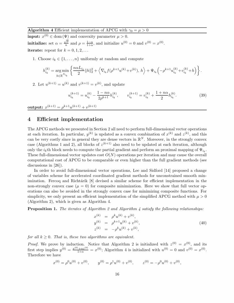
Algorithm 4 Efficient implementation of APCG with γ0 = µ > 0
input: x(0) ∈ dom (Ψ) and convexity parameter µ > 0.
initialize: set α =√µn and ρ = 1−α
1+α , and initialize u(0) = 0 and v(0) = x(0).
iterate: repeat for k = 0, 1, 2, . . .
1. Choose ik ∈ {1, . . . , n} uniformly at random and compute
h(k)ik
= argminh∈RNi
k
{nαLik
2‖h‖22 +
⟨
∇ikf(ρk+1u(k)+v(k)), h
⟩
+Ψik
(
−ρk+1u(k)ik
+v(k)ik
+h)}
.
2. Let u(k+1) = u(k) and v(k+1) = v(k), and update
u(k+1)ik
= u(k)ik
− 1− nα
2ρk+1h(k)ik
, v(k+1)ik
= v(k)ik
+1 + nα
2h(k)ik
. (39)
output: x(k+1) = ρk+1u(k+1) + v(k+1)
4 Efficient implementation
The APCGmethods we presented in Section 2 all need to perform full-dimensional vector operationsat each iteration. In particular, y(k) is updated as a convex combination of x(k) and z(k), and thiscan be very costly since in general they are dense vectors in R
N . Moreover, in the strongly convexcase (Algorithms 1 and 2), all blocks of z(k+1) also need to be updated at each iteration, althoughonly the ikth block needs to compute the partial gradient and perform an proximal mapping of Ψik .These full-dimensional vector updates cost O(N) operations per iteration and may cause the overallcomputational cost of APCG to be comparable or even higher than the full gradient methods (seediscussions in [26]).
In order to avoid full-dimensional vector operations, Lee and Sidford [14] proposed a changeof variables scheme for accelerated coordinated gradient methods for unconstrained smooth min-imization. Fercoq and Richtarik [8] devised a similar scheme for efficient implementation in thenon-strongly convex case (µ = 0) for composite minimization. Here we show that full vector op-erations can also be avoided in the strongly convex case for minimizing composite functions. Forsimplicity, we only present an efficient implementation of the simplified APCG method with µ > 0(Algorithm 2), which is given as Algorithm 4.
Proposition 1. The iterates of Algorithm 2 and Algorithm 4 satisfy the following relationships:
x(k) = ρku(k) + v(k),
y(k) = ρk+1u(k) + v(k), (40)
z(k) = −ρku(k) + v(k),
for all k ≥ 0. That is, these two algorithms are equivalent.
Proof. We prove by induction. Notice that Algorithm 2 is initialized with z(0) = x(0), and its
first step implies y(0) = x(0)+αz(0)
1+α = x(0); Algorithm 4 is initialized with u(0) = 0 and v(0) = x(0).Therefore we have
x(0) = ρ0u(0) + v(0), y(0) = ρ1u(0) + v(0), z(0) = −ρ0u(0) + v(0),
16
which means that (40) holds for k = 0. Now suppose that it holds for some k ≥ 0, then
(1− α)z(k) + αy(k) = (1− α)(
−ρku(k) + v(k))
+ α(
ρk+1u(k) + v(k))
= −ρk ((1− α)− αρ) u(k) + (1− α)v(k) + αv(k)
= −ρk+1u(k) + v(k). (41)
So h(k)ik
in Algorithm 4 can be written as
h(k)ik
= argminh∈RNik
{nαLik
2‖h‖22 + 〈∇ikf(y
(k)), h〉 +Ψik
(
(1− α)z(k)ik
+ αy(k)ik
+ h)}
.
Comparing with (11), and using βk = α, we obtain
h(k)ik
= z(k+1)ik
−((1− α)z
(k)ik
+ αy(k)ik
).
In terms of the full dimensional vectors, using (12) and (41), we have
z(k+1) = (1− α)z(k) + αy(k) + Uikh(k)ik
= −ρk+1u(k) + v(k) + Uikh(k)ik
= −ρk+1u(k) + v(k) +1− nα
2Uikh
(k)ik
+1 + nα
2Uikh
(k)ik
= −ρk+1
(
u(k) − 1− nα
2ρk+1Uikh
(k)ik
)
+
(
v(k) +1 + nα
2Uikh
(k)ik
)
= −ρk+1u(k+1) + v(k+1).
Using Step 3 of Algorithm 2, we get
x(k+1) = y(k) + nα(z(k+1) − z(k)) + nα2(z(k) − y(k))
= y(k) + nα(
z(k+1) −((1− α)z(k) + αy(k)
))
= y(k) + nαUikh(k)ik
,
where the last step used (12). Now using the induction hypothesis y(k) = ρk+1u(k) + v(k), we have
x(k+1) = ρk+1u(k) + v(k) +1− nα
2Uikh
(k)ik
+1 + nα
2Uikh
(k)ik
= ρk+1
(
u(k) − 1− nα
2ρk+1Uikh
(k)ik
)
+
(
v(k) +1 + nα
2Uikh
(k)ik
)
= ρk+1u(k+1) + v(k+1).
Finally,
y(k+1) =1
1 + α
(
x(k+1) + αz(k+1))
=1
1 + α
(
ρk+1u(k+1) + v(k+1))
+α
1 + α
(
−ρk+1u(k+1) + v(k+1))
=1− α
1 + αρk+1u(k+1) +
1 + α
1 + αv(k+1)
= ρk+2u(k+1) + v(k+1).
We just showed that (40) also holds for k + 1. This finishes the induction.
17
We note that in Algorithm 4, only a single block coordinates of the vectors u(k) and v(k)
are updated at each iteration, which cost O(Nik). However, computing the partial gradient∇ikf(ρ
k+1u(k)+v(k)) may still cost O(N) in general. In Section 5.2, we show how to further exploitproblem structure in regularized empirical risk minimization to completely avoid full-dimensionalvector operations.
5 Application to regularized empirical risk minimization (ERM)
In this section, we show how to apply the APCG method to solve the regularized ERM problemsassociated with linear predictors.
Let A1, . . . , An be vectors in Rd, φ1, . . . , φn be a sequence of convex functions defined on R,
and g be a convex function defined on Rd. The goal of regularized ERM with linear predictors is
to solve the following (convex) optimization problem:
minimizew∈Rd
{
P (w)def=
1
n
n∑
i=1
φi(ATi w) + λg(w)
}
, (42)
where λ > 0 is a regularization parameter. For binary classification, given a label bi ∈ {±1} foreach vector Ai, for i = 1, . . . , n, we obtain the linear SVM (support vector machine) problem bysetting φi(z) = max{0, 1 − biz} and g(w) = (1/2)‖w‖22 . Regularized logistic regression is obtainedby setting φi(z) = log(1 + exp(−biz)). This formulation also includes regression problems. Forexample, ridge regression is obtained by setting φi(z) = (1/2)(z − bi)
2 and g(w) = (1/2)‖w‖22 , andwe get the Lasso if g(w) = ‖w‖1. Our method can also be extended to cases where each Ai is amatrix, thus covering multiclass classification problems as well (see, e.g., [39]).
For each i = 1, . . . , n, let φ∗i be the convex conjugate of φi, that is,
φ∗i (u) = max
z∈R{zu− φi(z)}.
The dual of the regularized ERM problem (42), which we call the primal, is to solve the problem(see, e.g., [40])
maximizex∈Rn
{
D(x)def=
1
n
n∑
i=1
−φ∗i (−xi)− λg∗
(1
λnAx
)}
, (43)
where A = [A1, . . . , An]. This is equivalent to minimize F (x)def= −D(x), that is,
minimizex∈Rn
{
F (x)def=
1
n
n∑
i=1
φ∗i (−xi) + λg∗
(1
λnAx
)}
. (44)
The structure of F (x) above matches our general formulation of minimizing composite convexfunctions in (1) and (2) with
f(x) = λg∗(
1
λnAx
)
, Ψ(x) =1
n
n∑
i=1
φ∗i (−xi). (45)
Therefore, we can directly apply the APCG method to solve the problem (44), i.e., to solve the dualof the regularized ERM problem. Here we assume that the proximal mappings of the conjugate
18
functions φ∗i can be computed efficiently, which is indeed the case for many regularized ERM
problems (see, e.g., [40, 39]).In order to obtain accelerated linear convergence rates, we make the following assumption.
Assumption 3. Each function φi is 1/γ smooth, and the function g has unit convexity parameter 1.
Here we slightly abuse the notation by overloading γ and λ, which appeared in Sections 2and 3. In this section γ represents the (inverse) smoothness parameter of φi, and λ denotes theregularization parameter on g. Assumption 3 implies that each φ∗
i has strong convexity parameter γ(with respect to the local Euclidean norm) and g∗ is differentiable and∇g∗ has Lipschitz constant 1.
In order to match the condition in Assumption 2, i.e., f(x) needs to be strongly convex, we canapply the technique in Section 2.2 to relocate the strong convexity from Ψ to f . Without loss ofgenerality, we can use the following splitting of the composite function F (x) = f(x) + Ψ(x):
f(x) = λg∗(
1
λnAx
)
+γ
2n‖x‖22, Ψ(x) =
1
n
n∑
i=1
(
φ∗(−xi)−γ
2‖xi‖22
)
. (46)
Under Assumption 3, the function f is smooth and strongly convex and each Ψi, for i = 1, . . . , n,is still convex. As a result, we have the following complexity guarantee when applying the APCGmethod to minimize the function F (x) = −D(x).
Theorem 2. Suppose Assumption 3 holds and ‖Ai‖2 ≤ R for all i = 1, . . . , n. In order to obtainan expected dual optimality gap E[D⋆ −D(x(k))] ≤ ǫ using the APCG method, it suffices to have
k ≥(
n+
√
nR2
λγ
)
log(C/ǫ). (47)
where D⋆ = maxx∈Rn D(x) and
C = D⋆ −D(x(0)) +γ
2n‖x(0) − x⋆‖22. (48)
Proof. First, we notice that the function f(x) defined in (46) is differentiable. Moreover, for anyx ∈ R
n and hi ∈ R,
‖∇if(x+ Uihi)−∇if(x)‖2 =
∥∥∥∥
1
nAT
i
[
∇g∗(
1
λnA(x+ Uihi)
)
−∇g∗(
1
λnAx
)]
+γ
nhi
∥∥∥∥2
≤ ‖Ai‖2n
∥∥∥∥∇g∗
(1
λnA(x+ Uihi)
)
−∇g∗(
1
λnAx
)∥∥∥∥2
+γ
n‖hi‖2
≤ ‖Ai‖2n
∥∥∥∥
1
λnAihi
∥∥∥∥2
+γ
n‖hi‖2
≤(‖Ai‖22
λn2+
γ
n
)
‖hi‖2,
where the second inequality used the assumption that g has convexity parameter 1 and thus ∇g∗
has Lipschitz constant 1. The coordinate-wise Lipschitz constants as defined in Assumption 1 are
Li =‖Ai‖22λn2
+γ
n≤ R2 + λγn
λn2, i = 1, . . . , n.
19
The function f has convexity parameter γn with respect to the Euclidean norm ‖ · ‖2. Let µ be its
convexity parameter with respect to the norm ‖ · ‖L defined in (6). Then
µ ≥ γ
n
/R2 + λγn
λn2=
λγn
R2 + λγn.
According to Theorem 1, the APCG method converges geometrically:
E[
D⋆ −D(x(k))]
≤(
1−√µ
n
)k
C ≤ exp
(
−√µ
nk
)
C,
where the constant C is given in (48). Therefore, in order to obtain E[D⋆−D(x(k))] ≤ ǫ, it sufficesto have the number of iterations k to be larger than
n√µlog(C/ǫ) ≤ n
√
R2 + λγn
λγnlog(C/ǫ) =
√
n2 +nR2
λγlog(C/ǫ) ≤
(
n+
√
nR2
λγ
)
log(C/ǫ).
This finishes the proof.
Let us compare the result in Theorem 2 with the complexity of solving the dual problem (44)using the accelerated full gradient (AFG) method of Nesterov [27]. Using the splitting in (45)
and under Assumption 3, the gradient ∇f(x) has Lipschitz constant‖A‖22λn2 , where ‖A‖2 denotes the
spectral norm of A, and Ψ(x) has convexity parameter γn with respect to ‖ · ‖2. So the condition
number of the problem is
κ =‖A‖22λn2
/γ
n=
‖A‖22λγn
.
Suppose each iteration of the AFG method costs as much as n times of the APCG method (as wewill see in Section 5.2), then the complexity of the AFG method [27, Theorem 6] measured in termsof number of coordinate gradient steps is
O(n√κ log(1/ǫ)
)= O
√
n‖A‖22λγ
log(1/ǫ)
≤ O
(√
n2R2
λγlog(1/ǫ)
)
.
The inequality above is due to ‖A‖22 ≤ ‖A‖2F ≤ nR2. Therefore in the ill-conditioned case (assuming
n ≤ R2
λγ ), the complexity of AFG can be a factor of√n worse than that of APCG.
Several state-of-the-art algorithms for regularized ERM, including SDCA [40], SAG [35, 37] andSVRG [11, 48], have the iteration complexity
O
((
n+R2
λγ
)
log(1/ǫ)
)
.
Here the ratio R2
λγ can be interpreted as the condition number of the regularized ERM problem (42)and its dual (43). We note that our result in (47) can be much better for ill-conditioned problems,
i.e., when the condition number R2
λγ is much larger than n.Most recently, Shalev-Shwartz and Zhang [39] developed an accelerated SDCA method which
achieves the same complexity O((
n+√
nλγ
)
log(1/ǫ))
as our method. Their method is an inner-
outer iteration procedure, where the outer loop is a full-dimensional accelerated gradient method
20
in the primal space w ∈ Rd. At each iteration of the outer loop, the SDCA method [40] is called to
solve the dual problem (43) with customized regularization parameter and precision. In contrast,our APCG method is a straightforward single loop coordinate gradient method.
We note that the complexity bound for the aforementioned work are either for the primaloptimality P (w(k)) − P ⋆ (SAG and SVRG) or for the primal-dual gap P (w(k)) −D(x(k)) (SDCAand accelerated SDCA). Our results in Theorem 2 are in terms of the dual optimality D⋆−D(x(k)).In Section 5.1, we show how to recover primal solutions with the same order of convergence rate. InSection 5.2, we show how to exploit problem structure of regularized ERM to compute the partialgradient ∇if(x), which together with the efficient implementation proposed in Section 4, completelyavoid full-dimensional vector operations. The experiments in Section 5.3 illustrate that our methodhas superior performance in reducing both the primal objective value and the primal-dual gap.
5.1 Recovering the primal solution
Under Assumption 3, the primal problem (42) and dual problem (43) each has a unique solution,say w⋆ and x⋆, respectively. Moreover, we have P (w⋆) = D(x⋆). With the definition
ω(x) = ∇g∗(
1
λnAx
)
, (49)
we have w⋆ = ω(x⋆). When applying the APCGmethod to solve the dual regularized ERM problem,which generate a dual sequence x(k), we can obtain a primal sequence w(k) = ω(x(k)). Here wediscuss the relationship between the primal-dual gap P (w(k)) − D(x(k)) and the dual optimalityD⋆ −D(x(k)).
Let a = (a1, . . . , an) be a vector in Rn. We consider the saddle-point problem
maxx
mina,w
{
Φ(x, a,w)def=
1
n
n∑
i=1
φi(ai) + λg(w) − 1
n
n∑
i=1
xi(ATi w − ai)
}
, (50)
so that
D(x) = mina,w
Φ(x, a,w).
Given an approximate dual solution x(k) (generated by the APCG method), we can find a pair ofprimal solutions (a(k), w(k)) = argmina,w Φ(x(k), a, w), or more specifically,
a(k)i = argmax
ai
{
−x(k)i ai − φi(ai)
}
∈ ∂φ∗i (−x
(k)i ), i = 1, . . . , n, (51)
w(k) = argmaxw
{
wT
(1
λnAx(k)
)
− g(w)
}
= ∇g∗(
1
λnAx(k)
)
. (52)
As a result, we obtain a subgradient of D at x(k), denoted D′(x(k)), and
‖D′(x(k))‖22 =1
n2
n∑
i=1
(
ATi w
(k) − a(k)i
)2. (53)
We note that ‖D′(x(k))‖22 is not only a measure of the dual optimality of x(k), but also a measureof the primal feasibility of (a(k), w(k)). In fact, it can also bound the primal-dual gap, which is theresult of the following lemma.
21
Lemma 4. Given any dual solution x(k), let (a(k), w(k)) be defined as in (51) and (52). Then
P (w(k))−D(x(k)) ≤ 1
2nγ
n∑
i=1
(
ATi w
(k) − a(k)i
)2=
n
2γ‖D′(x(k))‖22.
Proof. Because of (51), we have ∇φi(a(k)i ) = −x
(k)i . The 1/γ-smoothness of φi(a) implies
P (w(k)) =1
n
n∑
i=1
φi(ATi w
(k)) + λg(w(k))
≤ 1
n
n∑
i=1
(
φi(a(k)i ) +∇φi(a
(k)i )T
(
ATi w
(k) − a(k)i
)
+1
2γ
(
ATi w
(k) − a(k)i
)2)
+ λg(w(k))
=1
n
n∑
i=1
(
φi(a(k)i )− x
(k)i
(
ATi w
(k) − a(k)i
)
+1
2γ
(
ATi w
(k) − a(k)i
)2)
+ λg(w(k))
= Φ(x(k), a(k), w(k)) +1
2nγ
n∑
i=1
(
ATi w
(k) − a(k)i
)2
= D(x(k)) +1
2nγ
n∑
i=1
(ATi w
(k) − a(k)i )2,
which leads to the inequality in the conclusion. The equality in the conclusion is due to (53).
The following theorem states that under a stronger assumption than Assumption 3, the primal-dual gap can be bounded directly by the dual optimality gap, hence they share the same order ofconvergence rate.
Theorem 3. Suppose g is 1-strongly convex and each φi is 1/γ-smooth and also 1/η-stronglyconvex (all with respect to the Euclidean norm ‖ · ‖2). Given any dual point x(k), let the primalcorrespondence be w(k) = ω(x(k)), i.e., generated from (52). Then we have
P (w(k))−D(x(k)) ≤ ληn+ ‖A‖22λγn
(
D⋆ −D(x(k)))
, (54)
where ‖A‖2 denotes the spectral norm of A.
Proof. Since g(w) is 1-strongly convex, the function f(x) = λg∗(Axλn
)is differentiable and ∇f(x)
has Lipschitz constant‖A‖22λn2 . Similarly, since each φi is 1/η strongly convex, the function Ψ(x) =
1n
∑ni=1 φ
∗i (−xi) is differentiable and ∇Ψ(x) has Lipschitz constant η
n . Therefore, the function−D(x) = f(x) + Ψ(x) is smooth and its gradient has Lipschitz constant
‖A‖22λn2
+η
n=
ληn+ ‖A‖22λn2
.
It is known that (e.g., [25, Theorem 2.1.5]) if a function F (x) is convex and L-smooth, then
F (y) ≥ F (x) +∇F (x)T (y − x) +1
2L‖∇F (x)−∇F (y)‖22
22
for all x, y ∈ Rn. Applying the above inequality to F (x) = −D(x), we get for all x and y,
−D(y) ≥ −D(x)−∇D(x)T (y − x) +λn2
2(ληn + ‖A‖22)‖∇D(x)−∇D(y)‖22. (55)
Under our assumptions, the saddle-point problem (50) has a unique solution (x⋆, a⋆, w⋆), wherew⋆ and x⋆ are the solutions to the primal and dual problems (42) and (43), respectively. Moreover,they satisfy the optimality conditions
ATi w
⋆ − a⋆i = 0, a⋆i = ∇φ∗i (−x⋆i ), w⋆ = ∇g∗
(1
λnAx⋆
)
.
Since D is differentiable in this case, we have D′(x) = ∇D(x) and ∇D(x⋆) = 0. Now we choose xand y in (55) to be x⋆ and x(k) respectively. This leads to
‖∇D(x(k))‖22 = ‖∇D(x(k))−∇D(x⋆)‖22 ≤ 2(ληn + ‖A‖22)λn2
(D(x⋆)−D(x(k))).
Then the conclusion can be derived from Lemma 4.
The assumption that each φi is 1/γ-smooth and 1/η-strongly convex implies that γ ≤ η.
Therefore the coefficient on the right-hand side of (54) satisfiesληn+‖A‖22
λγn > 1. This is consis-
tent with the fact that for any pair of primal and dual points w(k) and x(k), we always haveP (w(k))−D(x(k)) ≥ D⋆ −D(x(k)).
Corollary 1. Under the assumptions of Theorem 3, in order to obtain an expected primal-dual gapE[P (w(k))−D(x(k))
]≤ ǫ using the APCG method, it suffices to have
k ≥(
n+
√
nR2
λγ
)
log
((ληn+ ‖A‖22)
λγn
C
ǫ
)
,
where the constant C is defined in (48).
The above results require that each φi be both smooth and strongly convex. One example thatsatisfies such assumptions is ridge regression, where φi(ai) =
12(ai − bi)
2 and g(w) = 12‖w‖22. For
problems that only satisfy Assumption 3, we may add a small strongly convex term 12η (A
Ti w)
2 to
each loss φi(ATi w), and obtain that the primal-dual gap (of a slightly perturbed problem) share the
same accelerated linear convergence rate as the dual optimality gap. Alternatively, we can obtainthe same guarantee with the extra cost of a proximal full gradient step. This is summarized in thefollowing theorem.
Theorem 4. Suppose Assumption 3 holds. Given any dual point x(k), define
T (x(k)) = arg minx∈Rn
{
〈∇f(x(k)), x〉+ ‖A‖222λn2
‖x− x(k)‖22 +Ψ(x)
}
, (56)
where f and Ψ are defined in the simple splitting (45). Let
w(k) = ω(T (x(k))) = ∇g∗(
1
λnAT (x(k))
)
. (57)
Then we have
P (w(k))−D(T (x(k))) ≤ 4‖A‖22λγn
(
D(x⋆)−D(x(k)))
. (58)
23
Proof. Notice that the Lipschitz constant of ∇f(x) is Lf =‖A‖22λn2 , which is used in calculating
T (x(k)). The corresponding gradient mapping [27] at x(k) is
G(x(k)) = Lf
(
x(k) − T (x(k)))
=‖A‖22λn2
(
x(k) − T (x(k)))
.
According to [27, Theorem 1], we have
∥∥∥D′
(
T (x(k)))∥∥∥
2
2≤ 4
∥∥∥G(x(k))
∥∥∥
2
2≤ 8Lf
(
D(x⋆)−D(x(k)))
=8‖A‖22λn2
(
D(x⋆)−D(x(k)))
.
The conclusion can then be derived from Lemma 4.
Here the coefficient in the right-hand side of (58),4‖A‖22λγn , can be less than 1. This does not
contradict with the fact that the primal-dual gap should be no less than the dual optimality gap,because the primal-dual gap on the left-hand side of (58) is measured at T (x(k)) rather than x(k).
Corollary 2. Suppose Assumption 3 holds. In order to obtain a primal-dual pair w(k) and x(k)
such that E[P (w(k))−D(T (x(k)))
]≤ ǫ, it suffices to run the APCG method for
k ≥(
n+
√
nR2
λγ
)
log
(4‖A‖22λγn
C
ǫ
)
steps and follow with a proximal full gradient step (56) and (57), where C is defined in (48).
We note that the computational cost of the proximal full gradient step (56) is comparablewith n proximal coordinate gradient steps. Therefore the overall complexity of of this scheme ison the same order as necessary for the expected dual optimality gap to reach ǫ. Actually thenumerical experiments in Section 5.3 show that running the APCG method alone without the finalfull gradient step is sufficient to reduce the primal-dual gap at a very fast rate.
5.2 Implementation details
Here we show how to exploit the structure of the regularized ERM problem to efficiently computethe coordinate gradient ∇ikf(y
(k)), and totally avoid full-dimensional updates in Algorithm 4.We focus on the special case g(w) = 1
2‖w‖22 and show how to compute ∇ikf(y(k)). In this case,
g∗(v) = 12‖v‖22 and ∇g∗(·) is the identity map. According to (46),
∇ikf(y(k)) =
1
λn2AT
ik(Ay(k)) +
γ
ny(k)ik
.
Notice that we do not form y(k) in Algorithm 4. By Proposition 1, we have
y(k) = ρk+1u(k) + v(k).
So we can store and update the two vectors
p(k) = Au(k), q(k) = Av(k),
and obtainAy(k) = ρk+1p(k) + q(k).
24
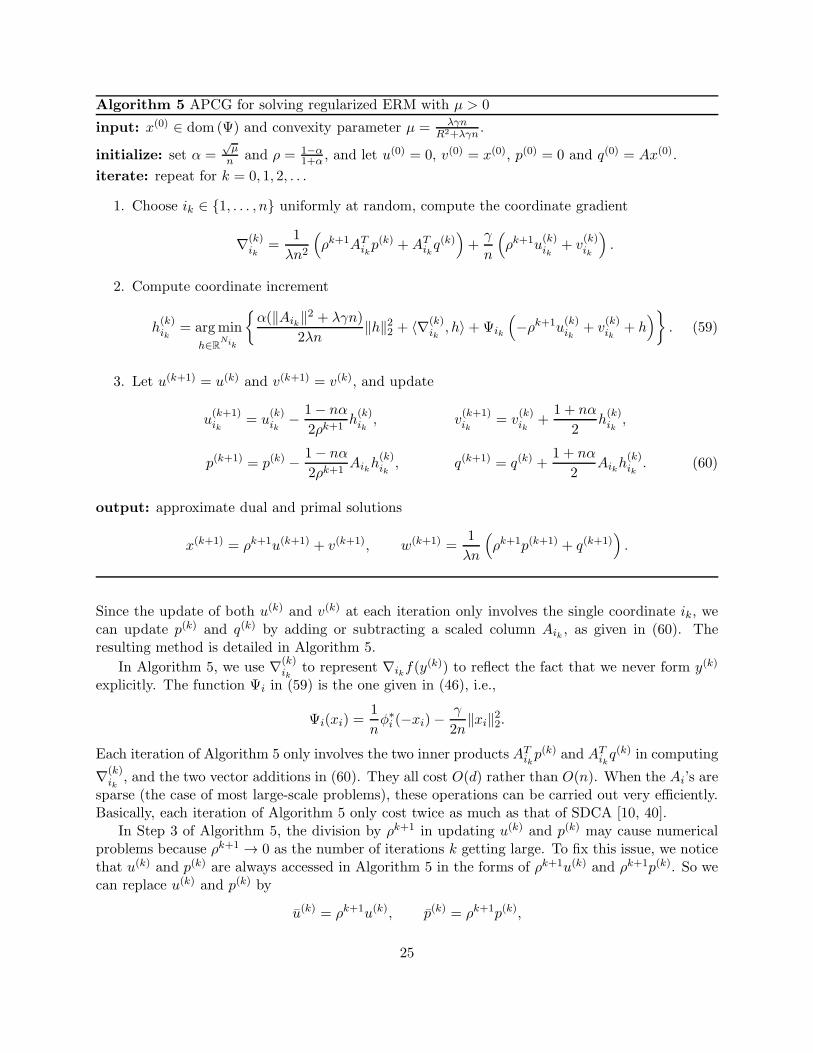
Algorithm 5 APCG for solving regularized ERM with µ > 0
input: x(0) ∈ dom (Ψ) and convexity parameter µ = λγnR2+λγn
.
initialize: set α =√µn and ρ = 1−α
1+α , and let u(0) = 0, v(0) = x(0), p(0) = 0 and q(0) = Ax(0).
iterate: repeat for k = 0, 1, 2, . . .
1. Choose ik ∈ {1, . . . , n} uniformly at random, compute the coordinate gradient
∇(k)ik
=1
λn2
(
ρk+1ATikp(k) +AT
ikq(k))
+γ
n
(
ρk+1u(k)ik
+ v(k)ik
)
.
2. Compute coordinate increment
h(k)ik
= argminh∈RNi
k
{α(‖Aik‖2 + λγn)
2λn‖h‖22 + 〈∇(k)
ik, h〉+Ψik
(
−ρk+1u(k)ik
+ v(k)ik
+ h)}
. (59)
3. Let u(k+1) = u(k) and v(k+1) = v(k), and update
u(k+1)ik
= u(k)ik
− 1− nα
2ρk+1h(k)ik
, v(k+1)ik
= v(k)ik
+1 + nα
2h(k)ik
,
p(k+1) = p(k) − 1− nα
2ρk+1Aikh
(k)ik
, q(k+1) = q(k) +1 + nα
2Aikh
(k)ik
. (60)
output: approximate dual and primal solutions
x(k+1) = ρk+1u(k+1) + v(k+1), w(k+1) =1
λn
(
ρk+1p(k+1) + q(k+1))
.
Since the update of both u(k) and v(k) at each iteration only involves the single coordinate ik, wecan update p(k) and q(k) by adding or subtracting a scaled column Aik , as given in (60). Theresulting method is detailed in Algorithm 5.
In Algorithm 5, we use ∇(k)ik
to represent ∇ikf(y(k)) to reflect the fact that we never form y(k)
explicitly. The function Ψi in (59) is the one given in (46), i.e.,
Ψi(xi) =1
nφ∗i (−xi)−
γ
2n‖xi‖22.
Each iteration of Algorithm 5 only involves the two inner products ATikp(k) and AT
ikq(k) in computing
∇(k)ik
, and the two vector additions in (60). They all cost O(d) rather than O(n). When the Ai’s aresparse (the case of most large-scale problems), these operations can be carried out very efficiently.Basically, each iteration of Algorithm 5 only cost twice as much as that of SDCA [10, 40].
In Step 3 of Algorithm 5, the division by ρk+1 in updating u(k) and p(k) may cause numericalproblems because ρk+1 → 0 as the number of iterations k getting large. To fix this issue, we noticethat u(k) and p(k) are always accessed in Algorithm 5 in the forms of ρk+1u(k) and ρk+1p(k). So wecan replace u(k) and p(k) by
u(k) = ρk+1u(k), p(k) = ρk+1p(k),
25
which can be updated without numerical problem. To see this, we have
u(k+1) = ρk+2u(k+1)
= ρk+2
(
u(k) − 1− nα
2ρk+1Uikh
(k)ik
)
= ρ
(
u(k) − 1− nα
2Uikh
(k)ik
)
.
Similarly, we have
p(k+1) = ρ
(
p(k) − 1− nα
2Aikh
(k)ik
)
.
5.3 Numerical experiments
In our experiments, we solve the regularized ERM problem (42) with smoothed hinge loss for binaryclassification. That is, we pre-multiply each feature vector Ai by its label bi ∈ {±1} and let
φi(a) =
0 if a ≥ 1,1− a− γ
2 if a ≤ 1− γ,12γ (1− a)2 otherwise,
i = 1, . . . , n.
The conjugate function of φi is φ∗i (b) = b+ γ
2 b2 if b ∈ [−1, 0] and ∞ otherwise. Therefore we have
Ψi(xi) =1
n
(
φ∗i (−xi)−
γ
2‖xi‖22
)
=
{ −xi
n if xi ∈ [0, 1]∞ otherwise.
For the regularization term, we use g(w) = 12‖w‖22. We used three publicly available datasets
obtained from [7]. The characteristics of these datasets are summarized in Table 1.In our experiments, we comparing the APCG method (Algorithm 5) with SDCA [40] and the
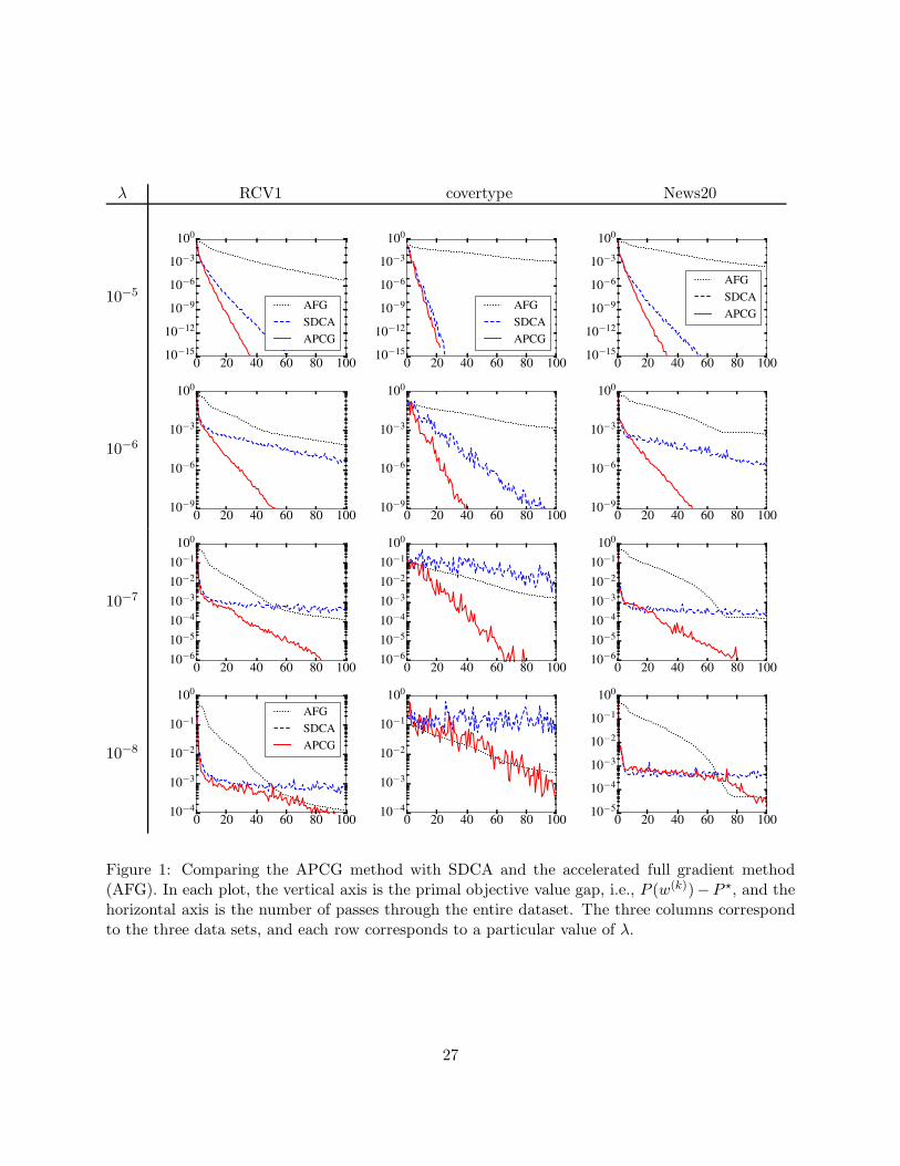
accelerated full gradient method (AFG) [25] with and additional line search procedure to improveefficiency. When the regularization parameter λ is not too small (around 10−4), then APCGperforms similarly as SDCA as predicted by our complexity results, and they both outperformAFG by a substantial margin.
Figure 1 shows the reduction of primal optimality P (w(k)) − P ⋆ by the three methods in theill-conditioned setting, with λ varying form 10−5 to 10−8. For APCG, the primal points w(k)
are generated simply as w(k) = ω(x(k)) defined in (49). Here we see that APCG has superiorperformance in reducing the primal objective value compared with SDCA and AFG, even withoutperforming the final proximal full gradient step described in Theorem 4.
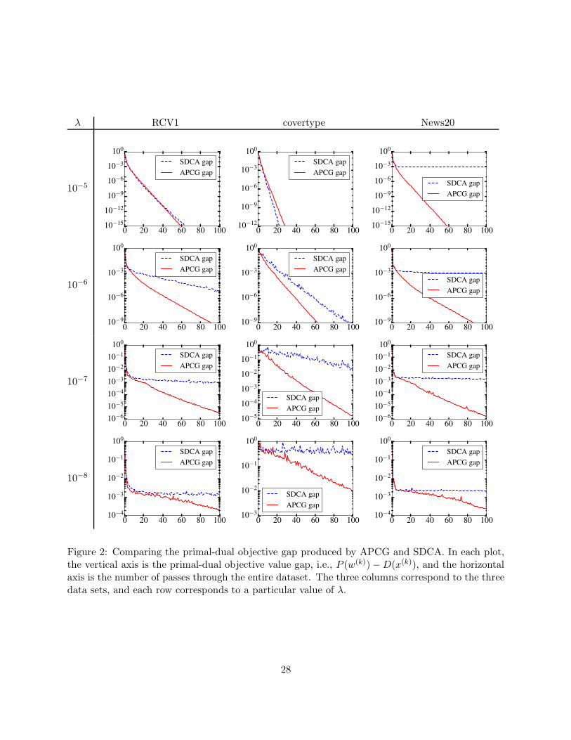
Figure 2 shows the reduction of primal-dual gap P (w(k))−D(x(k)) by the two methods APCGand SDCA. We can see that in the ill-conditioned setting, the APCG method is more effective inreducing the primal-dual gap as well.
datasets source number of samples n number of features d sparsity
RCV1 [16] 20,242 47,236 0.16%covtype [4] 581,012 54 22%News20 [12, 13] 19,996 1,355,191 0.04%
Table 1: Characteristics of three binary classification datasets obtained from [7].
26
λ RCV1 covertype News20
10−5
0 20 40 60 80 10010
−15
10−12
10−9
10−6
10−3
100
AFG
SDCA
APCG
0 20 40 60 80 10010
−15
10−12
10−9
10−6
10−3
100
AFG
SDCA
APCG
0 20 40 60 80 10010
−15
10−12
10−9
10−6
10−3
100
AFG
SDCA
APCG
10−6
0 20 40 60 80 10010
−9
10−6
10−3
100
0 20 40 60 80 10010
−9
10−6
10−3
100
0 20 40 60 80 10010
−9
10−6
10−3
100
10−7
0 20 40 60 80 10010
−6
10−5
10−4
10−3
10−2
10−1
100
0 20 40 60 80 10010
−6
10−5
10−4
10−3
10−2
10−1
100
0 20 40 60 80 10010
−6
10−5
10−4
10−3
10−2
10−1
100
10−8
0 20 40 60 80 10010
−4
10−3
10−2
10−1
100
AFG
SDCA
APCG
0 20 40 60 80 10010
−4
10−3
10−2
10−1
100
0 20 40 60 80 10010
−5
10−4
10−3
10−2
10−1
100
Figure 1: Comparing the APCG method with SDCA and the accelerated full gradient method(AFG). In each plot, the vertical axis is the primal objective value gap, i.e., P (w(k))−P ⋆, and thehorizontal axis is the number of passes through the entire dataset. The three columns correspondto the three data sets, and each row corresponds to a particular value of λ.
27
λ RCV1 covertype News20
10−5
0 20 40 60 80 10010−15
10−12
10−9
10−6
10−3
100
SDCA gap
APCG gap
0 20 40 60 80 10010−12
10−9
10−6
10−3
100
SDCA gap
APCG gap
0 20 40 60 80 10010−15
10−12
10−9
10−6
10−3
100
SDCA gap
APCG gap
10−6
0 20 40 60 80 10010−9
10−6
10−3
100
SDCA gap
APCG gap
0 20 40 60 80 10010−9
10−6
10−3
100
SDCA gap
APCG gap
0 20 40 60 80 10010−9
10−6
10−3
100
SDCA gap
APCG gap
10−7
0 20 40 60 80 10010−6
10−5
10−4
10−3
10−2
10−1
100
SDCA gap
APCG gap
0 20 40 60 80 10010−5
10−4
10−3
10−2
10−1
100
SDCA gap
APCG gap
0 20 40 60 80 10010−6
10−5
10−4
10−3
10−2
10−1
100
SDCA gap
APCG gap
10−8
0 20 40 60 80 10010−4
10−3
10−2
10−1
100
SDCA gap
APCG gap
0 20 40 60 80 10010−3
10−2
10−1
100
SDCA gap
APCG gap
0 20 40 60 80 10010−4
10−3
10−2
10−1
100
SDCA gap
APCG gap
Figure 2: Comparing the primal-dual objective gap produced by APCG and SDCA. In each plot,the vertical axis is the primal-dual objective value gap, i.e., P (w(k))−D(x(k)), and the horizontalaxis is the number of passes through the entire dataset. The three columns correspond to the threedata sets, and each row corresponds to a particular value of λ.
28
References
[1] A. Beck and M. Teboulle. A fast iterative shrinkage-threshold algorithm for linear inverseproblems. SIAM Journal on Imaging Sciences, 2(1):183–202, 2009.
[2] A. Beck and L. Tetruashvili. On the convergence of block coordinate descent type methods.SIAM Journal on Optimization, 13(4):2037–2060, 2013.
[3] D. P. Bertsekas and J. N. Tsitsiklis. Parallel and Distributed Computation: Numerical Methods.Prentice-Hall, 1989.
[4] J. A. Blackard, D. J. Dean, and C. W. Anderson. Covertype data set. In K. Bache andM. Lichman, editors, UCI Machine Learning Repository, URL: http://archive.ics.uci.edu/ml,2013. University of California, Irvine, School of Information and Computer Sciences.
[5] J. K. Bradley, A. Kyrola, D. Bickson, and C. Guestrin. Parallel coordinate descent for l1-regularized loss minimization. In Proceedings of the 28th International Conference on MachineLearning (ICML), pages 321–328, 2011.
[6] K.-W. Chang, C.-J. Hsieh, and C.-J. Lin. Coordinate descent method for large-scale l2-losslinear support vector machines. Journal of Machine Learning Research, 9:1369–1398, 2008.
[7] R.-E. Fan and C.-J. Lin. LIBSVM data: Classification, regression and multi-label. URL:http://www.csie.ntu.edu.tw/˜cjlin/libsvmtools/datasets, 2011.
[8] O. Fercoq and P. Richtarik. Accelerated, parallel and proximal coordinate descent. Manuscript,arXiv:1312.5799.
[9] M. Hong, X. Wang, M. Razaviyayn, and Z. Q. Luo. Iteration complexity analysis of blockcoordinate descent methods. arXiv:1310.6957.
[10] C.-J. Hsieh, K.-W. Chang, C.-J. Lin, S. S. Keerthi, and S. Sundararajan. A dual coordinatedescent method for large-scale linear svm. In Proceedings of the 25th International Conferenceon Machine Learning (ICML), pages 408–415, 2008.
[11] R. Johnson and T. Zhang. Accelerating stochastic gradient descent using predictive variancereduction. In Advances in Neural Information Processing Systems 26, pages 315–323. 2013.
[12] S. S. Keerthi and D. DeCoste. A modified finite Newton method for fast solution of large scalelinear svms. Journal of Machine Learning Research, 6:341–361, 2005.
[13] K. Lang. Newsweeder: Learning to filter netnews. In Proceedings of the Twelfth InternationalConference on Machine Learning (ICML), pages 331–339, 1995.
[14] Y. T. Lee and A. Sidford. Efficient accelerated coordinate descent methods and faster algo-rithms for solving linear systems. arXiv:1305.1922.
[15] D. Leventhal and A. S. Lewis. Randomized methods for linear constraints: convergence ratesand conditioning. Mathematics of Operations Research, 35(3):641–654, 2010.
[16] D. D. Lewis, Y. Yang, T. Rose, and F. Li. RCV1: A new benchmark collection for textcategorization research. Journal of Machine Learning Research, 5:361–397, 2004.
29
[17] Y. Li and S. Osher. Coordinate descent optimization for ℓ1 minimization with application tocompressed sensing: a greedy algorithm. Inverse Problems and Imaging, 3:487–503, 2009.
[18] J. Liu and S. J. Wright. An accelerated randomized Kacamarz algorithm. arXiv:1310.2887,2013.
[19] J. Liu, S. J. Wright, C. Re, V. Bittorf, and S. Sridhar. An asynchronous parallel stochasticcoordinate descent algorithm. JMLR W&CP, 32(1):469–477, 2014.
[20] Z. Lu and L. Xiao. On the complexity analysis of randomized block-coordinate descent meth-ods. Technical Report MSR-TR-2013-53, Microsoft Research, 2013.
[21] Z. Lu and L. Xiao. Randomized block coordinate non-monotone gradient method for a classof nonlinear programming. arXiv:1306.5918, 2013.
[22] Z. Q. Luo and P. Tseng. On the convergence of the coordinate descent method for convexdifferentiable minimization. Journal of Optimization Theory and Applications, 72(1):7–35,2002.
[23] I. Necoara and D. Clipici. Distributed random coordinate descent method for compositeminimization. Technical Report 1-41, University Politehnica Bucharest, November 2013.
[24] I. Necoara and A. Patrascu. A random coordinate descent algorithm for optimization problemswith composite objective function and linear coupled constraints. Computational Optimizationand Applications, 57(2):307–377, 2014.
[25] Y. Nesterov. Introductory Lectures on Convex Optimization: A Basic Course. Kluwer, Boston,2004.
[26] Y. Nesterov. Efficiency of coordinate descent methods on huge-scale optimization problems.SIAM Journal on Optimization, 22(2):341–362, 2012.
[27] Yu. Nesterov. Gradient methods for minimizing composite functions. Mathematical Program-ming, Ser. B, 140:125–161, 2013.
[28] A. Patrascu and I. Necoara. Efficient random coordinate descent algorithms for large-scale structured nonconvex optimization. To appear in Journal of Global Optimization.arXiv:1305.4027, 2013.
[29] J. Platt. Fast training of support vector machine using sequential minimal optimization. InB. Scholkopf, C. Burges, and A. Smola, editors, Advances in Kernel Methods — Support VectorLearning, pages 185–208. MIT Press, Cambridge, MA, USA, 1999.
[30] Z. Qin, K. Scheinberg, and D. Goldfarb. Efficient block-coordinate descent algorithms for theGroup Lasso. Mathematical Programming Computation, 5(2):143–169, 2013.
[31] P. Richtarik and M. Takac. Parallel coordinate descent methods for big data optimization.arXiv:1212.0873, 2012.
[32] P. Richtarik and M. Takac. Distributed coordinate descent method for learning with big data.arXiv:1310.2059, 2013.
30
[33] P. Richtarik and M. Takac. Iteration complexity of randomized block-coordinate descentmethods for minimizing a composite function. Mathematical Programming, 144(1):1–38, 2014.
[34] R. T. Rockafellar. Convex Analysis. Princeton University Press, 1970.
[35] N. Le Roux, M. Schmidt, and F. Bach. A stochastic gradient method with an exponentialconvergence rate for finite training sets. In Advances in Neural Information Processing Systems25, pages 2672–2680. 2012.
[36] A. Saha and A. Tewari. On the non-asymptotic convergence of cyclic coordinate descentmethods. SIAM Jorunal on Optimization, 23:576–601, 2013.
[37] M. Schmidt, N. Le Roux, and F. Bach. Minimizing finite sums with the stochastic averagegradient. Technical Report HAL 00860051, INRIA, Paris, France, 2013.
[38] S. Shalev-Shwartz and A. Tewari. Stochastic methods for ℓ1 regularized loss minimization. InProceedings of the 26th International Conference on Machine Learning (ICML), pages 929–936,Montreal, Canada, 2009.
[39] S. Shalev-Shwartz and T. Zhang. Accelerated proximal stochastic dual coordinate ascent forregularized loss minimization. arXiv:1309.2375.
[40] S. Shalev-Shwartz and T. Zhang. Stochastic dual coordinate ascent methods for regularizedloss minimization. Journal of Machine Learning Research, 14:567–599, 2013.
[41] P. Tseng. Convergence of a block coordinate descent method for nondifferentiable minimiza-tion. Journal of Optimization Theory and Applications, 140:513–535, 2001.
[42] P. Tseng. On accelerated proximal gradient methods for convex-concave optimization. Un-published manuscript, 2008.
[43] P. Tseng and S. Yun. Block-coordinate gradient descent method for linearly constrainednonsmooth separable optimization. Journal of Optimization Theory and Applications, 140:513–535, 2009.
[44] P. Tseng and S. Yun. A coordinate gradient descent method for nonsmooth separable mini-mization. Mathematical Programming, 117:387–423, 2009.
[45] Z. Wen, D. Goldfarb, and K. Scheinberg. Block coordinate descent methods for semidefiniteprogramming. In M. F. Anjos and J. B. Lasserre, editors, Handbook on Semidefinite, Coneand Polynomial Optimization: Theory, Algorithms, Software and Applications, volume 166,pages 533–564. Springer, 2012.
[46] S. J. Wright. Accelerated block-coordinate relaxation for regularized optimization. SIAMJournal on Optimization, 22:159–186, 2012.
[47] T. Wu and K. Lange. Coordinate descent algorithms for Lasso penalized regression. TheAnnals of Applied Statistics, 2(1):224–244, 2008.
[48] L. Xiao and T. Zhang. A proximal stochastic gradient method with progressive variancereduction. arXiv:1403.4699.
31