An untargeted LC-MS investigation of South African

An untargeted LC-MS investigation of South African children with respiratory

chain deficiencies

Leonie Venter

B.Sc. Hons. Biochemistry

21834350

Dissertation submitted in fulfilment of the requirements for the degree Magister Scientiae in Biochemistry at the

Potchefstroom Campus of the North-West University

Supervisor: Dr R Louw

Co-supervisor: Dr Z Lindeque

Assistant Supervisor: Prof I Smuts

May 2014

i

ABSTRACT

Mitochondria are the main site of cellular adenosine triphosphate (ATP) generation which is

achieved by a series of multi-subunit complexes and electron carriers which together create the

oxidative phosphorylation system (OXPHOS). Whenever a defect in any of the numerous

mitochondrial pathways occurs it is commonly referred to as a mitochondrial disorder.

Mitochondrial disorders are a heterogeneous group of disorders characterised by impaired

energy production and include a wide range of defects of either mitochondrial DNA (mtDNA) or

nuclear DNA (nDNA) encoded proteins. In cases of dysfunction in the respiratory chain

(complex I to IV) it is known to be a respiratory chain deficiency (RCD) which presents a huge

challenge for routine diagnosis largely due to the lack of a specific and sensitive biomarker(s).

One sure way of confirming the suspicion of a RCD is by performing enzyme analysis on a

muscle sample obtained through a biopsy. However, due to the lack of theatre time available to

clinicians and the relative large number of false positive patients that are being selected for

biopsies, it was decided to develop a biosignature to limit the number of false positive patients

from the diagnostic workflow.

An untargeted liquid chromatography mass spectrometry (LC-MS) metabolomics approach was

used to investigate RCDs in children from South Africa. Sample preparation, a liquid

chromatography time-of-flight mass spectrometry method and data processing methods were

standardised. Furthermore the developed methodology made use of reverse phase

chromatography in conjunction with positive electrospray ionisation (ESI) and a hydrophilic

interaction chromatography (HILIC) in negative electrospray ionisation. Urine samples of 61

patients representing three different experimental groups were analysed. The three

experimental groups comprised of patients with respiratory chain deficiencies, clinical referred

controls (CRC) and patients suffering from various neuromuscular disorders (NMD). After a

variety of data mining steps and statistical analysis a list of 12 features were compiled with the

ability to distinguish between patients with RCDs and CRCs. The proposed signature was also

tested on the neuromuscular disorder group, but this result indicated that the biosignature

performed better when used to differentiate between patients with RCDs and CRCs, since the

model was designed with this purpose. An alternative validation study is required to identify the

features found with this proposed biosignature, to ensure that this biosignature can be

practically implemented as a non-invasive screening method.

KEY TERMS: respiratory chain deficiency; metabolomics; urinary biomarker; LC-MS.

ii

WEES GEDULDIG

Alles gebeur op sy tyd.

Die windpomp gaan soek nie die wind nie.

iii

ACKNOWLEDGEMENTS

I would like to express my sincerest gratitude to the following people (institutions) who played an

important role in this project of mine:

Firstly, thank you to Dr Roan Louw for all your patience, support and guidance. You assisted

through all the highs and lows of this project, even though some situations needed a ―sterk

koppie koffie‖ you never gave up on me, thank you.

Thanks to Dr Zander Lindeque for helping me, time after time, after time, after time. Your efforts

went beyond the call of duty. I’m not sure how you do all you do and know all you know, but I’m

really glad you were on my team.

To Prof Izelle Smuts, I thank you for all your assistance regarding patient selection and collection.

Thank you for making us realise that there are real people out there living with illnesses – we

indeed have so much to be grateful for.

Thank you to Mr Peet Jansen van Rensburg for being willing to help me 24 hours a day. Your

advice and knowledge came in very handy. I’m sure that the Q-TOF and TOF will never be the

same again...

To my fellow members of the Mitochondrial Research Laboratory, without you guys most days

would surely have been beyond dull. Thanks for making this a memorable year.

To the members of the BOSS lab, thank you for always welcoming me into your laboratory with a

smile.

Thank you to the kind people at Zoology for allowing me to use their WONDERFULL Q-TOF at

such a crucial time.

Thank you to the National Research Foundation and the NWU Postgraduate fund for financial

assistance.

Ms Karlien Badenhorst thank you to for the language and spelling editing of my dissertation.

A huge word of thanks to my family and friends. Without all your love, support and prayers this

would have been much harder. I’m blessed to have you all in my life.

Finally I would like to thank our Heavenly Father for making all of this possible. “For I know the

plans I have for you, declares the Lord, plans to prosper you and not to harm you, plans to give

you hope and a future.” – Jeremiah 29:11.

iv

TABLE OF CONTENTS

ABSTRACT ................................................................................................................................ i

ACKNOWLEDGEMENTS .......................................................................................................... iii

LIST OF FIGURES ................................................................................................................... viii

LIST OF TABLES ...................................................................................................................... x

ABBREVIATIONS ..................................................................................................................... xi

CHAPTER 1 ............................................................................................................................. 1

Introduction ............................................................................................................................ 1

PROBLEM STATEMENT ........................................................................................................ 2

AIM AND OBJECTIVES .......................................................................................................... 3

STRUCTURE OF STUDY ....................................................................................................... 3

CHAPTER 2 ............................................................................................................................. 5

Literature review .................................................................................................................... 5

2.1 THE MITOCHONDRION ................................................................................................... 6

2.2 OXIDATIVE PHOSPHORYLATION .................................................................................. 8

2.3 mtDNA AND nDNA ........................................................................................................... 9

2.4 DAMAGING THE MITOCHONDRION ............................................................................. 11

2.5 MITOCHONDRIAL DISEASE.......................................................................................... 12

2.6 RESPIRATORY CHAIN DEFICIENCIES ........................................................................ 13

2.7 DIAGNOSING MITOCHONDRIAL DEFECTS ................................................................. 14

2.7.1 Clinical criteria .......................................................................................................... 15

2.7.2 Biochemical and/or histochemical investigations ...................................................... 16

2.7.3 Molecular investigations ........................................................................................... 21

2.8 TREATMENT OPTIONS ................................................................................................. 21

2.9 NEXT STEP FOR RCD ................................................................................................... 23

2.10 METABOLOMICS ......................................................................................................... 23

2.11 EXPERIMENTAL APPROACH ..................................................................................... 26

CHAPTER 3 ........................................................................................................................... 28

Untargeted positive ESI LC-MS assay ............................................................................. 28

3.1 INTRODUCTION ............................................................................................................ 29

v

3.2 REAGENTS AND BUFFERS .......................................................................................... 29

3.2.1 Q-TOF reagents ....................................................................................................... 29

3.2.2 Amino acid preparation ............................................................................................. 29

3.2.3 Organic acid preparation .......................................................................................... 30

3.2.4 Internal standard preparation .................................................................................... 30

3.3 INSTRUMENTATION ..................................................................................................... 30

3.3.1 LC-Q-TOF ................................................................................................................ 30

3.4 REVERSE PHASE CHROMATOGRAPHIC SEPARATION ............................................ 31

3.5 ORGANIC ACID EXTRACTION ...................................................................................... 31

3.6 DATA EXTRACTION PROCESS .................................................................................... 32

3.7 METHOD DEVELOPMENT ............................................................................................ 33

3.7.1 Different data extraction methods (MFE vs. FbI) ....................................................... 34

3.7.2 Different sample preparation methods ...................................................................... 41

3.8 STANDARDISED LC-Q-TOF METHOD FOR POSITIVE ESI.......................................... 50

CHAPTER 4 ........................................................................................................................... 52

Untargeted negative ESI LC-MS assay ............................................................................ 52

4.1 INTRODUCTION ............................................................................................................ 53

4.2 REAGENTS AND BUFFERS .......................................................................................... 53

4.2.1 Q-TOF reagents ....................................................................................................... 53

4.2.2 Standard preparation ................................................................................................ 53

4.2.3 Internal standard preparation .................................................................................... 54

4.3 INSTRUMENTATION ..................................................................................................... 54

4.3.1. LC-QQQ .................................................................................................................. 54

4.3.2. LC-Q-TOF ............................................................................................................... 55

4.4 CHROMATOGRAPHIC SEPARATION ........................................................................... 56

4.4.1 Reverse phase chromatography ............................................................................... 56

4.4.2 Hydrophilic interaction chromatography .................................................................... 56

4.5 DATA EXTRACTION ...................................................................................................... 57

4.6 TUNING AND CALIBRATION ......................................................................................... 57

4.7 METHOD DEVELOPMENT ............................................................................................ 58

4.7.1 Different mobile phase modifiers .............................................................................. 58

4.7.2 Hydrophilic interaction chromatography (HILIC) ....................................................... 65

4.8 STANDARDISED LC-Q-TOF ASSAY FOR NEGATIVE ESI ........................................... 74

vi

CHAPTER 5 ........................................................................................................................... 76

Metabolomics investigation of respiratory chain deficient patients ......................... 76

5.1 INTRODUCTION ............................................................................................................ 77

5.2 SAMPLE SELECTION .................................................................................................... 77

5.2.1 Ethical aspects ......................................................................................................... 78

5.2.2 Experimental groups ................................................................................................. 78

5.2.3 Selection criteria ....................................................................................................... 80

5.3 METABOLOMICS SAMPLE PREPARATION AND ANALYSIS ....................................... 81

5.4 QUALITY CONTROL ...................................................................................................... 83

5.5 DATA ANALYSIS ............................................................................................................ 83

5.5.1 Raw data .................................................................................................................. 84

5.5.2 Data extraction ......................................................................................................... 84

5.5.3 Data pre-processing and normalisation .................................................................... 85

5.5.4 Data pre-treatment ................................................................................................... 87

5.5.5 Statistical analysis: Feature selection and biomarker testing ................................... 88

5.6 FEATURE IDENTIFICATION .......................................................................................... 93

5.7 RESULTS AND DISCUSSIONS ..................................................................................... 93

5.7.1 Positive electrospray ionisation data quality.............................................................. 93

5.7.2 Negative electrospray ionisation data quality ............................................................ 95

5.7.3 Overview of data before feature selection ................................................................. 98

5.7.4 Univariate and multivariate feature selection .......................................................... 101

5.7.5 Final feature selection ............................................................................................ 103

5.7.6 Proposed biosignature ............................................................................................ 105

5.7.7 Evaluating the signature’s discrimination power ..................................................... 107

5.8 IMPLEMENTING THE SIGNATURE ON A PRACTICAL EXAMPLE ............................. 112

CHAPTER 6 ......................................................................................................................... 116

Conclusion .......................................................................................................................... 116

6.1 INTRODUCTION .......................................................................................................... 117

6.2 CONCLUSIONS............................................................................................................ 117

6.2.1 Standardisation procedures .................................................................................... 117

6.2.2 Experimental group selection and analysis ............................................................. 119

6.2.3 Feature selection .................................................................................................... 120

6.2.4 Biomarker discovery ............................................................................................... 120

6.2.5 Biosignature evaluation .......................................................................................... 121

vii

6.2.6 Final conclusion ...................................................................................................... 122

6.3 FUTURE RECOMMENDATIONS ................................................................................. 122

CHAPTER 7 ......................................................................................................................... 124

References .......................................................................................................................... 124

ANNEXURE A ..................................................................................................................... 133

Importance of univariate and multivariate statistics .................................................. 133

IMPORTANCE OF METABOLITE COVARIANCE AND MULTIVARIATE STATISTICS ...... 134

APPENDIX A ....................................................................................................................... 136

List of features ................................................................................................................... 136

111 FEATURES FOUND TO BE IMPORTANT BY UNIVARIATE AND MULTIVARIATE

STATISTICAL METHODS .................................................................................................. 137

viii

LIST OF FIGURES

Figure 2.1: The internal structure of mitochondria .................................................................... 7

Figure 2.2: Oxidative phosphorylation ...................................................................................... 9

Figure 2.3: Diagnostic approach for identifying suspected mitochondrial defects ................... 15

Figure 2.4: Systems biology illustrated by the different ―omics‖ .............................................. 24

Figure 2.5: Experimental approach workflow ......................................................................... 26

Figure 3.1: Recursive data extraction workflow of untargeted metabolomics data .................... 33

Figure 3.2: Illustration of different aspects to investigate with positive ESI ............................... 34

Figure 3.3: MFE CV distribution. .............................................................................................. 37

Figure 3.4: MFE followed by FbI CV distribution ....................................................................... 38

Figure 3.5: PCA score plots of different data extraction methods ............................................. 40

Figure 3.6: Workflow of sample preparation methods ............................................................... 43

Figure 3.7: Multivariate visualisation of urine prepared with different methods ......................... 44

Figure 3.8: Data plot representation of the normalised variables present in six different samples obtained with positive ESI 45

Figure 3.9: Multivariate visualisation of spiked* and unspiked urine samples analysed with both positive and negative ESI ....................................................................................... 48

Figure 3.10: Workflow followed for sample analysis using positive ESI .................................... 50

Figure 4.1: Summary of steps to follow for experimentation using negative ESI. ................... 58

Figure 4.2: PCA plots based on features found after basic data manipulations. ..................... 63

Figure 4.3: Chromatographic illustration of uracil ................................................................... 69

Figure 4.4: Chromatographic illustration of adenosine. .......................................................... 70

Figure 4.5: Chromatographic illustration of nor-leucine. ......................................................... 70

Figure 4.6: PCA display of HILIC column analysis. ................................................................ 72

Figure 4.7: Sample workflow for negative ESI. ....................................................................... 74

Figure 5.1: Experimental groups representing the samples used for LC-Q-TOF analysis. ..... 79

Figure 5.2: Data mining process. ........................................................................................... 84

Figure 5.3: List of statistical analyses performed.................................................................... 89

Figure 5.4: PCA score plots of the positive ESI data indicating the sample batches .............. 94

Figure 5.5: Alternative display of positive ESI QC sample position. ....................................... 95

Figure 5.6: PCA score plots representing sample batches analysed with negative ES .......... 96

Figure 5.7: Negative ESI QC sample distribution ................................................................... 97

ix

Figure 5.8: Overview PCA score plot before feature selection process .................................. 98

Figure 5.9: Multivariate-AUC before feature selection. ......................................................... 100

Figure 5.10: Average predictive accuracies during model cross validation with different number

of features. ......................................................................................................... 100

Figure 5.11: Univariate and multivariate Venn diagrams of features with significance. ........... 102

Figure 5.12: Combined Venn diagram of features found. ....................................................... 103

Figure 5.13: Graph display of feature ranking. ....................................................................... 104

Figure 5.14: PCA score plot of the proposed signature. ......................................................... 107

Figure 5.15: ROC curve for the proposed biosignature .......................................................... 108

Figure 5.16: Average predicted class probability of RCDs and clinical referred controls over 100

cross validations ................................................................................................ 109

Figure 5.17: Permutation test of the proposed biosignature. .................................................. 111

Figure 5.18: 3D PCA score plot of the three experimental groups analysed .......................... 112

Figure 5.19: AUC of patients with neuromuscular disorders ................................................... 114

Figure A.1: Univariate vs multivariate approaches. ............................................................... 134

x

LIST OF TABLES

Table 3.1: MFE compound example ........................................................................................ 36

Table 3.2: Combined MFE and FbI compound example .......................................................... 36

Table 3.3: Indication of the features detected in normal and spiked urine samples .................. 46

Table 4.1: MRM conditions used to detect uracil, nor-leucine and adenosine .......................... 55

Table 4.2: Data manipulations ................................................................................................. 60

Table 4.3: Effect of different mobile phase ratios on retention time .......................................... 68

Table 5.1: Experimental group compilation .............................................................................. 80

Table 5.2: Metabolite markers identified ................................................................................ 105

Table 5.3: Two-class confusion matrix ................................................................................... 110

xi

ABBREVIATIONS

A:

a.a: Amino acids

ACN: Acetonitrile

ADP: Adenosine diphosphate

AMP: Adenosine monophosphate

ANT: Adenine nucleotide translocase

ATP: Adenosine triphosphate

AUC: Area under the curve

B:

BAER: Brainstem auditory evoked responses

C:

CEF: Compound Exchange Format

CE-MS: Capillary electrophoresis mass spectrometry

CNS: Central nervous system

CoA: Coenzyme A

Complex 1: NADH coenzyme Q reductase

Complex 2: Succinate-CoQ reductase complex

Complex 3: Reduced CoQ cytochrome c reductase complex

Complex 4: Cytochrome c oxidase

Complex 5: ATP synthase complex

CoQ: Coenzyme Q

COX: Cytochrome c oxidase

CRC: Clinical referred control

CS: Citrate synthase

CSF: Cerebrospinal fluid

CT: Computed tomography

CuSOD: Copper superoxide dismutase

CV: Coefficient of variation

CXR: Chest X-ray

Cyt c: Cytochrome c

CI-IV: Respiratory chain enzyme complexes I to IV respectively

xii

D:

DNA: Deoxyribonucleic acid

E:

e-: Electrons

EC: Electron complex

ECG: Electrocardiography

EMG: Electromyography

ES: Effect size

ESI: Electron spray ionisation

ETC: Electron transport chain

etc.: Et cetera

F:

FADH: Flavin adenine dinucleotide (reduced)

FbF: Find by formula

FbI: Find by Ion

FDA: Food and Drug Administration

FGF: Fibroblast growth factor

FMN: Flavin mononucleotide

FN: False negative

FP: False positive

G:

GC-MS: Gas chromatography mass spectrometer

Glog: Generalised logarithm

H:

HILIC: Hydrophilic interaction chromatography

HMDB: Human metabolome database

HPLC: High-performance liquid chromatography

H2O: Water

H2O2: Hydrogen peroxide

I:

IS: Internal standard

xiii

K:

kDa: Kilo Dalton

L:

L: Litre

LC: Liquid chromatography

LC-MS: Liquid chromatography mass spectrometry

LC-Q-TOF: Liquid chromatography quadrupole time-of-flight

LHON: Leber’s hereditary optic neuropathy

LS: Leigh Syndrome

M:

MCCV: Monte-Carlo cross validation

MDC: Mitochondrial resonance imaging

MELAS: Mitochondrial myopathy, encephalopathy, lactic acidosis, and stroke

syndrome

MERRF: Mitochondrial encephalomyopathy characterized by ragged red fibbers in

damaged muscle

METLIN: Metabolite and tandem MS database

MFE: Molecular Feature Extraction

mg: Milligrams

MilliQ: Millipore

MnSOD: Manganese superoxide dismutase

MPP: Mass profiler professional

MRI: Magnetic resonance imaging

MRM: Multiple reaction monitoring

MS: Mass spectrometry

MS/MS: Tandem mass spectrometry

MSTUS: Mass sprectra total useful signal

mtDNA: Mitochondrial deoxyribonucleic acid

MVI: Missing value imputation

m/z: Mass to charge

N:

NAD+: Nicotinamide adenine dinucleotide (oxidised)

NADH: Nicotinamide adenine dinucleotide (reduced)

xiv

NCS: Nerve conduction studies

nDNA: Nuclear deoxyribonucleic acid

NMD: Neuromuscular disorder

NMR: Nuclear magnetic resonance

O:

o.a: Organic acids

OAE: Organic acid extraction

OH-: Hydroxyl radical

OXPHOS: Oxidative phosphorylation

O2: Oxygen

O2-: Superoxide anion

P:

PC: Principal component

PCA: Principal component analyses

PCR: Polymerase chain reaction

PDH: Pyruvate dehydrogenase

PDHC: Pyruvate dehydrogenase complex

PLS-DA: Partial least square discriminant analysis

ppm: Parts per million

Q:

QC: Quality control

QQQ: Triple quad

Q-TOF: Quadrupole time of flight

R:

RC: Respiratory chain

RCD: Respiratory chain deficiency

RCDs: Respiratory chain deficiencies

RF: Random forest

RFLP: Restriction fragment length polymorphism

RNA: Ribonucleic acid

ROC: Receiving operating characteristic

ROCCET: ROC curve explorer and tester

ROS: Reactive oxygen species

xv

RP: Reverse phase

RRF: Ragged red fibers

RT: Retention time

S:

SDH: Succinate dehydrogenase

SVM: Support vector machine

T:

TCA: Tricarboxylic acid

TIM: Translocase of the inner membrane

TN: True negative

TOM: Translocase of the outer membrane

TP: True positive

tRNA: Transfer ribonucleic acid

V:

VEP: Visual evoked potentials

VIP: Variable important in projection

Z:

ZnSOD: Zinc superoxide dismutase

Symbols:

ß: Beta

µl: Microlitre

µm: Micrometre

Web servers:

HMDB (www.hmdb.ca)

Matlab (www.mathworks.com/matlab)

Metabo-analyst (www.metaboanalyst.ca)

METLIN (http://metlin.scripps.edu)

ROCCET (www.roccet.ca)

http://www.hmdb.ca/

http://www.mathworks.com/matlab

http://www.metaboanalyst.ca/

http://metlin.scripps.edu/

http://www.roccet.ca/

1

CHAPTER 1:

Introduction

Chapter 1

2

Mitochondria are unique cell organelles whose structure allows metabolism to take place in

eukaryotes. One of the main functions of the mitochondrion is to generate cellular energy in the

form of adenosine triphosphate mostly by means of the oxidative phosphorylation system by

using a series of multi-subunit enzyme complexes and electron carriers. Most OXPHOS

complexes are assembled from proteins encoded in both the nDNA and mtDNA. Once a

mutation occurs in any of the numerous proteins involved in mitochondrial energy metabolism, it

is referred to as a mitochondrial disorder. Mitochondrial diseases have a minimum prevalence

of 1 in 5 000 live births, and are now considered as the most common subgroup of inherited

metabolic diseases. Whenever a problem arises in the respiratory chain (complex I to IV) it is

known as a respiratory chain deficiency which ultimately leads to a decrease in ATP production.

Theoretically, this subgroup of mitochondrial disorders can give rise to any symptom, in any

organ or tissue at any age, due to combined involvement of Mendelian and mitochondrial

genetics.

PROBLEM STATEMENT

Diagnosis of mitochondrial disorders is complicated and requires a multidisciplinary approach

consisting of clinical, histochemical, biochemical and molecular assessments. When

diagnosing a patient with a suspected RCD, the most reliable method with the best success rate

remains to be enzyme analysis on a muscle biopsy sample. Muscle is mitochondria-rich tissue

and has a high energy demand. The fact that obtaining a muscle sample is a highly invasive

method which is usually done under anaesthetic brings its own limitations and difficulties. One

of the main research challenges is finding a screening method that is less invasive when it

comes to choosing the right candidates to undergo a muscle biopsy.

The use of metabolite biomarkers in bio-fluids (blood or urine) is less invasive, less expensive,

high throughput and could be useful in monitoring patients over time and during treatment.

Here metabolomics is playing a large role in the discovery of biomarkers or risk factors

associated with specific diseases, as well in gathering greater pathophysiologic understanding

of the onset and progression of diseases. In fact, metabolomics has been used in previous

investigations at the Biochemistry Department at the NWU to find a biosignature for RCD

consisting of six organic acids, six amino acids and creatine. However, these investigations

made use of more targeted screening methods with limited metabolome coverage. For this

Chapter 1

3

reason the quest to find other potential markers by using untargeted methods to distinguish

between RCD patients and clinically referred controls still needs to be completed.

AIM AND OBJECTIVES

Considering all the factors mentioned, the aim of this study was to use an untargeted LC-MS

metabolomics approach to investigate respiratory chain deficiencies in children from South

Africa. This approach creates a chance to find ―new‖ metabolites associated with RCD which

could differentiate between patients with RCDs and clinical referred controls. This aim will be

accomplished by completing the following objectives:

o Firstly there is a need to standardise both positive- and negative electrospray ionisation

techniques using a quadrupole time-of-flight mass spectrometer.

o Secondly it is necessary to analyse urine samples of children suffering from respiratory

chain deficiencies alongside urine from different control groups.

o Lastly the compilation of a list of features distinguishing RCD patients and clinical

referred controls from one another would be essential to confirm if the aim was

successfully reached.

STRUCTURE OF STUDY

Chapter 2 contains a literature review relevant to investigating respiratory chain deficiencies

with focus on the mitochondria, oxidative phosphorylation system, mitochondrial defects, most

important factors concerning respiratory chain deficiencies and metabolomics as a research

tool. A complete outline of the experimental approach is given at the end of this chapter.

Chapter 3 and Chapter 4 contains all the method development steps followed along with the

results obtained by reverse phase liquid chromatography with positive electrospray ionisation

and hydrophilic interaction chromatography with negative electrospray ionisation, respectively.

These chapters are concluded with a summary of the standardised methods for both

electrospray ionisation modes. Chapter 5 describes the investigation of RCD patient samples

with the standardised methods, followed by a constructed model with the potential of being used

as a diagnostic screening method. Chapter 6 is the concluding chapter, summarising the

findings and discussing their significance, followed by future prospects and recommendations

Chapter 1

4

for this research. All the references used to complete this study are listed in Chapter 7. An

annexure explaining why the use of both univariate and multivariate methods and an appendix

containing information of the features found using univariate and multivariate methods are

supplied as suffixes.

5

CHAPTER 2:

Literature review

Chapter 2

6

2.1 THE MITOCHONDRION

The mitochondrion is a membrane enclosed organelle found in virtually all eukaryotic cells, with

the exception being erythrocytes, and is generally referred to as the powerhouse of the cell. It

is currently believed that mitochondria are the offspring of aerobic bacteria which formed part of

an ancient prokaryote colony in the range of 1 to 3 billion years ago (Pieczenik and Neustadt,

2007). The cellular localisation of the mitochondrion depends on mitochondrial division, fusion,

motility and tethering. These are all activities which need to be regulated to ensure proper

functioning of the mitochondria (Nunnari and Suomalainen, 2012). The number of mitochondria

can range from hundreds to thousands per cell depending on the energy requirements of the

cell. Metabolic active cells like the skeletal- and cardiac muscle contains the largest number of

mitochondria due to the increased amount of substrate and oxygen utilised by these cells

(Bandyopadhyay and Dutta, 2010).

Structurally the mitochondrion can range from 0.5-1 μm in diameter and can be up to 7 μm long.

They are classified as a rod or sphere shaped like organelle (as illustrated in Figure 2.1). This

very complex organelle contains two phospholipid bilayers which can be categorised into 4

different segments: the outer membrane; the inner membrane; the inter membrane space; as

well as the matrix. The content of the outer membrane of the mitochondria is identical to the

plasma membrane and typically porous to ions and molecules that are less than 5 kilo Dalton

(KDa) to freely diffuse through it. The entry of larger proteins into the membrane is achieved

when binding to specific transporters known as translocase of the outer membrane (TOM) and

translocase of the inner membrane (TIM) which is located on the membrane. The inner

membrane encloses and twists into the mitochondrial matrix forming cristae, which increases

the inner membrane surface. The cristae membrane houses the protein sectors that shuttle

electrons, which arrive from the tricarboxylic acid (TCA) cycle and contribute to the energy

yielding process. Unlike the outer membrane the inner membrane is less porous to ions and

small molecules, which makes it an ideal space for compartmentalisation (Bolisetty and Jaimes,

2013). Furthermore, the inner membrane is an electrical insulator and chemical barrier, which

allows the exchange of anions between the cytosol and the mitochondrial matrix (O’Rourke et

al., 2005). It is suggested that the inter membrane space contributes to the maintenance of

mitochondrial homeostasis. The matrix contains a multitude of enzymes, proteins and peptides

as well as a genome that encodes for a few proteins and ribonucleic acid (RNA) molecules

necessary for translation (Bolisetty and Jaimes, 2013).

Chapter 2

7

Figure 2.1: The internal structure of mitochondria. The rod shape organelle containing an outer

membrane, inner membrane, and inter membrane space is clearly visible in the figure. Furthermore the

independent DNA, ribosomes and cristae folds are also illustrated (Adapted from Frey and Mannella,

2000).

Mitochondria perform a number of functions in humans. First and foremost the mitochondria

produce about 90% of the cellular energy in the form of adenosine triphosphate mostly by

means of the oxidative phosphorylation system (Pieczenik and Neustadt, 2007). The

mitochondrion is involved in mediation of intermediary metabolism, this includes: beta (β)-

oxidation; the citrate cycle; steroid metabolism; the uric acid cycle; decarboxylation of pyruvate

and the biosynthesis of heme; pyrimidines; amino acids; phospholipids; iron-sulphur clusters

and nucleotides (Bandyopadhyay and Dutta, 2010). Maintaining calcium homeostasis can also

be seen as a function of the mitochondria (Smeitink et al., 2006). In addition mitochondria plays

a part in cell signalling and triggering of cell death pathways, like apoptosis and necrosis (Saeed

and Singer, 2013). The production of heat is an alternative function mitochondria perform, by

the uncoupling of the OXPHOS system which leads to thermogenesis, particularly in brown fat

Chapter 2

8

of newborns. The mitochondria also contribute to heredity by means of its own

deoxyribonucleic acid (DNA) (Bandyopadhyay and Dutta, 2010). The electrochemical potential

of the inner-membrane generated by the OXHPOS system supports mitochondrial protein

import and also triggers changes on molecular level which may change mitochondrial behaviour

in a response to mitochondrial dysfunction. The supplementation of ATP and TCA cycle

intermediates to serve as building blocks for neurotransmitters can be seen as another function

of the mitochondria (Nunnari and Suomalainen, 2012). Taking the facts mentioned above into

consideration, and not excluding other possibilities, it is clear that the mitochondria fulfil a

number of important functions in eukaryotic cells.

2.2 OXIDATIVE PHOSPHORYLATION

Energy production, which is the main function of the mitochondria, is a result of two closely

integrated metabolic processes namely, the TCA cycle and the electron transport chain (ETC).

Under aerobic conditions glucose is metabolised to pyruvate by glycolysis in the cytosol. The

pyruvate is transported into the mitochondrial matrix where it is converted to acetyl coenzyme A

(acetyl CoA) by means of pyruvate dehydrogenase (Pieczenik and Neustadt, 2007). Fatty acids

on the other hand are esterified to fatty acyl CoA in the cytosol, where the medium chain fatty

acids can diffuse through the mitochondrial membrane and the long chain fatty acids depend on

the carnitine pathway to be transported. Once in the mitochondrial matrix the fatty acyl CoA

undergoes β-oxidation and produces acetyl CoA. Acetyl CoA feeds into the TCA cycle

generating the electron carriers, nicotinamide and flavin adenine dinucleotides (NADH and

FADH2). Ultimately the ETC which is embedded within the inner mitochondrial membrane

receives electrons thanks to NADH and FADH2 (Saeed and Singer, 2013). The ETC displayed

in Figure 2.2 consists of four multi-subunit protein complexes (I-IV), coenzyme Q, cytochrome c

(Cyt c), and along with complex V it is collectively known as the oxidative phosphorylation

system.

Complex I of the ETC receives electrons from NADH which is then oxidised to NAD+, while

complex II receives electrons from FADH2. The donated electrons are passed along to

ubiquinone (coenzyme Q) and then to complex III. Cytochrome c is an iron-containing heme

protein and transfer electrons from complex III to complex IV. At complex IV the electrons along

with hydrogen ions and oxygen is used to form water (H2O). As electrons transfer down the

ETC, protons move across the inner mitochondrial membrane through complexes I, III and IV,

resulting in the generation of an electrochemical gradient (Pieczenik and Neustadt, 2007).

Chapter 2

9

Consequently the gradient provides energy to drive the ATP synthase complex (complex V),

allowing protons to flow back into the inner mitochondrial membrane to produce ATP from

adenosine diphosphate (ADP). Finally matrix ATP is transferred out of the mitochondria and

with the help of adenine nucleotide translocase (ANT) exchanged for cytosolic ADP (Wallace

and Fan, 2010).

Figure 2.2: Oxidative phosphorylation. Redox reactions leading to the generation of a proton gradient

by means of complexes I, III and IV, along with proton backflow through complex V ultimately producing

ATP. Also shown is the main sites of reactive oxygen species (ROS) production, namely complex I and III

(Saeed and Singer, 2013).

2.3 mtDNA AND nDNA

The complexes of the OXPHOS system are manufactured from proteins encode by both nuclear

DNA and mitochondrial DNA. Communication between these two genomes is essential for

ideal assembly and functioning of the system. Complex I (NADH coenzyme Q reductase) which

is the first and the largest respiratory complex consist of approximately 46 subunits, of which 7

are encoded by mtDNA and 39 are encoded by nDNA. Complex II (succinate-CoQ reductase),

has 4 nDNA encoded subunits. Complex III (CoQ cytochrome c reductase) has 1 mtDNA

encoded subunit and 10 nDNA encoded subunits, adding to a total of 11 subunits. The fourth

Chapter 2

10

complex (cytochrome c oxidase) houses 13 subunits, where 3 of these subunits are mtDNA

encoded and the remaining 10 are nDNA encoded. Lastly complex V (ATP synthase) has

about 16 subunits of which 2 are mtDNA and 14 nDNA encoded (DiMauro and Schon, 2003,

Wallace and Fan, 2010). Mitochondrial DNA further encodes for 2 ribosomal and 22 transfer

ribonucleic acid (tRNA) necessary for mitochondrial translation. The remaining mitochondrial

proteins, OXPHOS assembly proteins and biosynthesis proteins are nuclear encoded and

transferred into the mitochondria (Smeitink et al., 2006).

It is commonly known that nuclear DNA wraps around histones to protect the DNA from damage

and to assist in the process of breaking double stranded DNA. Mitochondrial DNA on the

contrary is not protected by histones and lacks introns, which makes it more vulnerable to

damage (Neustadt and Pieczenik, 2008).

Most human cells contain two copies of nuclear DNA. Mitochondrial DNA can range from 1 000

to 100 000 copies depending on the cell type. Healthy individuals will have identical mtDNA at

birth referred to as homoplasmy (Chinnery and Schon, 2003). Once a mutation emerges in the

mtDNA a mixed population of normal and mutant mtDNA are created, this is known as

heteroplasmy. Division of a heteroplasmic cell results in the distribution of two types of mtDNA

into the daughter cells causing a genetic drift towards either pure mutant- or wild type mtDNA

(Wallace and Fan, 2010). The amount of mutated mtDNA varies among patients and also from

organ to organ and between cells within the same individual. The level of mutated mtDNA may

also change during development and throughout life, potentially influencing the phenotype

within an individual (DiMauro and Schon, 2003). As an increase in the number of mutant

pathogenic mtDNAs takes place, a decrease in mitochondrial function is apparent. When

energy output has become inadequate for normal cell functioning, a threshold is crossed

resulting in possible initiation of apoptosis or necrosis and symptom appearance (Wallace and

Fan, 2010).

According to Munnich et al., (2011) pathological alterations of mtDNA fall into three major

classes: point mutations, deletions/duplications and copy number mutations. Firstly, point

mutations are mainly maternally inherited, heteroplasmic, include amino acid substitutions and

proteins synthesis mutations. Secondly, deletions/duplications differ among patients but

frequently surround various coding and tRNA genes. These alterations are mostly unique,

sporadic, heteroplasmic and can be found between directly repeated sequences, suggesting it

is caused by De novo rearrangements that occur during oogenesis or early development.

Thirdly, mtDNA depletions due to copy number mutations are consistent with autosomal

http://click.thesaurus.com/click/nn1ov4?clksite=thes&clkpage=the&clkld=0&clkorgn=0&clkord=0&clkmod=1clk&clkitem=vulnerable&clkdest=http%3A%2F%2Fthesaurus.com%2Fbrowse%2Fvulnerable

Chapter 2

11

recessive inheritance and found in about 5% of patients, proposing that nuclear gene defects

are responsible for respiratory chain deficiencies (Munnich et al., 2011).

Nuclear DNA mutations associated with disease are divided into two classes. The first class

can be seen as mutations influencing assembly and maintenance protein genes. The second

class consist of mutations in nuclear encoded respiratory chain subunits. Only a hand full of

subunit gene mutations has been proclaimed to date. These mutations include a mutation in

the gene for complex II flavoprotein and nuclear-encoded complex I gene mutations (Munnich et

al., 2011).

2.4 DAMAGING THE MITOCHONDRION

Several sources can be accountable for abnormal mitochondrial functioning that leads to human

disease. Mutations of mtDNA and nDNA or changes due to free radical mediated damage or

faulty repairs can be seen as reasons (Schapira, 2012).

As a by-product of OXPHOS the mitochondria generate reactive oxygen species (ROS), which

is a highly regulated procedure under normal physiological conditions. The majority of ROS are

generated by complexes I and III likely due to electron leakage. Whenever the ETC becomes

reduced, the overflow of electrons passes directly to oxygen (O2) which produces a superoxide

anion (O2-). At complex I the O2

- which gets released into the mitochondrial matrix is converted

to hydrogen peroxide (H2O2) with the help of the matrix manganese superoxide dismutase

(MnSOD). At complex III the released superoxides are reformed to hydrogen peroxide (H2O2)

by copper/zinc superoxide dismutases (Cu/ZnSOD), H2O2 can be further reduced to hydroxyl

radical (OH-) (Wallace and Fan, 2010). Oxidative damage occurs and accumulates in the

mitochondria when enzymes cannot convert the superoxide radicals to H2O fast enough. Once

mitochondrial proteins are damaged their affinity for substrates or coenzymes decreases

ultimately decreasing their function (Neustadt and Pieczenik, 2008). Extravagant mitochondrial

ROS production may overwhelm the antioxidant defences of the cell, eventually leading to the

destruction of the cell (Wallace and Fan, 2010).

Minerals, vitamins and various metabolites which act as cofactors for the function and synthesis

of mitochondrial enzymes contribute to mitochondrial function. Whenever metabolic

deregulation occurs mitochondrial malfunction would likely follow. Deficiencies of any

component of the Krebs cycle or respiratory chain (RC) normally results in an increased free

http://click.thesaurus.com/click/nn1ov4?clksite=thes&clkpage=the&clkld=0&clkorgn=100074&clkord=0&clkmod=1clk&clkitem=extravagant&clkdest=http%3A%2F%2Fthesaurus.com%2Fbrowse%2Fextravagant%3Fo%3D100074

Chapter 2

12

radical production and finally mtDNA damage. Dysfunctional mitochondria may lead to a feed

forward process, where mitochondrial damage causes more damage (Pieczenik and Neustadt,

2007).

Assorted medications can directly and indirectly damage the mitochondria. In some cases

medication can inhibit mtDNA transcription of the ETC complexes, damaging other ETC

components resulting in inhibition of enzymes required for glycolysis and β-oxidation. Other

medications may cause the depletion of body nutrients by decreasing endogenous antioxidants

as a result of free radical production, finally leading to less than proper functioning of the ETC

complexes and/or mitochondrial enzymes (Neustadt and Pieczenik, 2008).

2.5 MITOCHONDRIAL DISEASE

Mitochondrial diseases include a clinically heterogeneous group of disorders with a minimum

prevalence of about 1 in every 5 000 live births (Schaefer et al., 2004). It is further estimated

that approximately 1 in 200 people are carriers of pathogenic mtDNA mutations (Diaz et al.,

2011). Defects in any of the numerous mitochondrial pathways due to spontaneous or inherited

mutations can cause a mitochondrial disease. This may include: respiratory chain deficiencies;

fatty acid oxidation disorders; Kerbs cycle and pyruvate dehydrogenase complex deficiencies

etc. (DiMauro and Schon, 2003).

In 1962 the first event of a mitochondrial disease was described by Luft and colleagues. This

event was based on a 35 year old female who suffered from myopathy, excessive perspiration,

heat intolerance, polydipsia with polyuria and a basal metabolic rate of 180% of normal. It was

stated that the patient suffered from uncoupling of the OXPHOS system (Luft et al., 1962).

Over the last 50 years mitochondrial dysfunction has been associated with a variety of

pathologic and toxicological conditions. These conditions may range from steatohepatitis,

acquired diseases (diabetes and atherosclerosis) and neurodegenerative diseases (Parkinson’s

and Alzheimer’s disease) to inherited diseases (Pieczenik and Neustadt, 2007).

Disorders of the mitochondria are commonly divided into primary and secondary mitochondrial

disorders. Primary mitochondrial disorders result from deficiencies of the OXPHOS system and

other mitochondrial proteins or enzymes such as the pyruvate dehydrogenase complex, TCA

cycle enzymes or mitochondrial carrier proteins (Smuts and van der Westhuizen, 2010). When

dysfunction occurs secondary due to an unrelated genetic or environmental cause it is referred

Chapter 2

13

to as a secondary mitochondrial disorder. In some cases ETC enzyme activity can be reduced

secondary to other metabolic diseases or due to sample handling errors (Haas et al., 2007).

When looking at primary mitochondrial disorders the majority of these disorders follow a pattern

of maternal or Mendelian inheritance. When studying paediatric patients with mitochondrial

diseases it is clear that a great part of these disorders are caused by nuclear DNA mutations

which follow an autosomal recessive inheritance pattern (Haas et al., 2007). Hence,

mitochondrial disorders may be from a nuclear or a mitochondrial origin and can be inherited in

a maternal, autosomal recessive, autosomal dominant or X-linked manor (Smuts and van der

Westhuizen, 2010).

Maternal inheritance refers to the fact that all mitochondria in the zygote derive from the ovum.

Therefore, a mother carrying a mtDNA mutation passes it on to all her children, but only her

daughters will transfer it to their progeny (Haas et al., 2007). Autosomal recessive inheritance

takes place when the nDNA is inherited from both parents, if both are carriers of the mutated

gene and not the disease. In the case of autosomal recessive inheritance, there is a 25%

chance of having a child with the disease, a 50% chance of having a child who is a carrier and a

25% chance of having a totally unaffected child. Autosomal dominant inheritance is completely

expressed in the heterozygote and will happen if one parent has a dominant nuclear DNA gene

mutation. This abnormal gene will be passed on to 50% of the children, regardless of gender

and regardless of whether the disease is fully developed. X-linked inheritance refers to those

recessive genes that reside on the X-chromosome (Harper, 2004).

2.6 RESPIRATORY CHAIN DEFICIENCIES

The mammalian mitochondrial proteome consist of approximately 1 100 proteins. This makes it

easy to believe that mitochondrion is the most structurally and functionally diverse cellular

organelles across species and within the same species across different tissues (Mannella et al.,

2013). The five protein complexes of the OXPHOS system can be seen as deficient when

mtDNA mutations or nuclear gene mutations encoding the OXPHOS proteins occur (Schapira,

2012). Whenever one of the four proteins that make up the respiratory chain becomes impaired

it is referred to as a respiratory chain deficiency (RCD), ultimately leading to a decrease in ATP

production. RCDs are classified as the largest subgroup of mitochondrial disorders

(Suomalainen, 2011b).

Chapter 2

14

A defect of the mitochondrial respiratory chain should be considered at any occasion where

combinations of unexplained neuromuscular and/or non-neuromuscular symptoms, with a

continuous course, including unrelated organs or tissues, are present in patients. Hypothetically

a RCD can give rise to any symptom in any organ at any age with any mode of inheritance.

Symptoms may include: hearing loss; ophthalmological abnormalities; muscle weakness;

neurological involvement; cardiac manifestations; gastrointestinal system problems; endocrine

abnormalities and renal involvement (Munnich et al., 2011).

2.7 DIAGNOSING MITOCHONDRIAL DEFECTS

Currently there is no uniform or standardised set of guidelines for the biochemical and

molecular evaluation of a suspected mitochondrial disease, which leads to different methods

being used by different laboratories worldwide (Smuts and van der Westhuizen, 2010).

Diagnosing a mitochondrial disease can be seen as difficult due to the diversity and often non-

specific presentations of these disorders. Adding to the difficulty is the absence of a specific

and reliable biomarker (Haas et al., 2007). Diagnosing a suspected mitochondrial disease is a

multi-disciplinary approach (summarised in Figure 2.3) which generally refers to three levels of

investigation that include: 1) clinical investigations; 2) biochemical and/or histochemical

investigations and 3) molecular investigations (Smuts and van der Westhuizen, 2010).

Chapter 2

15

Figure 2.3: Diagnostic approach for identifying suspected mitochondrial defects. The process

may include clinical, biochemical and molecular investigations.

2.7.1 Clinical criteria

Due to the fact that a mitochondrial disease can present at any age and is characterised by a

highly variable phenotype, it is quite difficult to diagnose patients according to symptoms

present. Mitochondrial disorders are usually presented with multi-systemic involvement. Well

established phenotypes like Leber’s Hereditary Optic Neuropathy (LHON) help to direct the

symptoms of a patient into a possible diagnosis, but the problem arises when the patient does

not fulfil the criteria for one of these syndromes. Scoring patients according to mitochondrial

disease criteria (which varies from institution to institution) may be a useful guideline towards a

preliminary prediction (Smuts and van der Westhuizen, 2010). Exercise testing like bicycle and

treadmill ergometry may accompany the clinical investigation (Haas et al., 2008). Brain imaging

is also used to confirm the possibility of nervous system involvement, which is quite common in

patients with mitochondrial disease (Haas et al., 2007).

Chapter 2

16

2.7.2 Biochemical and/or histochemical investigations

Before biochemical examination of muscle (obtained through a biopsy) is done, metabolite

analysis in blood and urine is generally carried out. Critical suggestions for the attendance of a

mitochondrial defect can be found in these results (Rodenburg, 2011).

2.7.2.1 Amino acid analysis

Different methodologies like ion exchange chromatography with post-column derivatisation,

tandem mass spectrometry (MS/MS) and reverse phase liquid chromatography are used when

analysing amino acids. When comparing alanine levels to the essential amino acids, lysine,

phenylalanine and tyrosine, the alanine findings can be an indication of a mitochondrial disease

when the absolute elevation in alanine is more than 450 μM in plasma. The elevated level of

alanine will be as a result of the transamination of pyruvate by alanine transferase. The

problem when using amino acid analysis is the low sensitivity of elevated alanine for

mitochondrial diseases. Alanine may be elevated under different conditions, for instance during

physiologic stress. Other amino acids whose elevations have been associated with

mitochondrial dysfunction include: proline; glycine; sarcosine and tyrosine (in newborn

screening studies). Amino acid analysis can be performed on blood, urine and cerebrospinal

fluid (CSF) (Haas et al., 2008, Rodenburg, 2011).

2.7.2.2 Organic acid analysis

Analysis of organic acids is largely performed by using a gas chromatography mass

spectrometer (GC-MS). Urine is the best sample to use for organic acid analysis due to its

higher extraction efficiency compared to plasma. During a period of clinical stability, urinary

organic acid analysis may have a low sensitivity for the detection of mitochondrial disease,

mainly because of the lack of symptoms often present in patients. When dealing with a

mitochondrial disease, increased excretions of TCA cycle intermediates like ethylmalonic acid

and 3-methyl-glutaconic acid commonly occur, but are seldom of any help from a diagnostic

point of view. TCA cycle intermediates are not solely increased in urine when a mitochondrial

disease is present, it may also be elevated due to renal immaturity. Dicarboxylic acidemia,

which is a result of microsomal fatty acid metabolism, is another common finding when

analysing urinary organic acids of patients with a mitochondrial disease. This organic acidemia

may arise from dietary artefact, prolonged fasting or drugs. Low muscle mass and creatine

Chapter 2

17

synthesis defects may indicate false elevations of organic acids due to the fact that the results

are normalised to the concentration of urine creatinine (Haas et al., 2008).

2.7.2.3 Carnitine analysis

Carnitine acts as a server of the mitochondrial shuttle for free fatty acids and it plays a role as

an acceptor of coenzyme A (CoA) esters. Identification of primary and secondary fatty acid

oxidation defects, carnitine deficiencies, and some amino- and organic acidemias can be done

by quantification of free carnitine levels and acyl-carnitine profiling in blood. Quantitative acyl-

carnitine analysis is done by liquid chromatography followed by electrospray ionisation mass

spectrometry. When quantification is done both the absolute values of the acyl-carnitine

species and the ratios of certain acyl-carnitine esters may be helpful towards a diagnosis. False

negatives in individuals with total carnitine deficiency may occur, which limits the test results

(Haas et al., 2008).

2.7.2.4 Lactate and pyruvate analysis

Lactate, a product of anaerobic glucose metabolism, accumulates when aerobic metabolism is

impaired, resulting in a shift in the oxidised-to-reduced NAD+/NADH ratio within mitochondria. A

decrease in this ratio goes along with a feedback inhibition of the pyruvate dehydrogenase

(PDH) complex, resulting in an increase in mitochondrial pyruvate value (Janssen et al., 2003).

Increased plasma lactate and/or pyruvate levels appear due to a wide range of factors like: the

result of physical exercise before sample collection; the ability of pyruvate increasing in the first

few hours after a meal in healthy individuals; poor sample handling and the possibility of

increased lactate concentrations in other metabolic diseases. An increase in ketone bodies (3-

hydroxybutyrate/acetoacetate) along with a secondary elevation of blood lactate may be present

in patients with RCD. Increased blood lactate, CSF lactate or lactate to pyruvate ratio, can

increase one’s suspicion of a RCD but can neither prove nor exclude it (Haas et al., 2008).

2.7.2.5 Other non-invasive analysis

Fibroblast growth factor 21 (FGF-21) which is a circulating hormone-like cytokine, regulator of

the starvation response and lipid metabolism has been reported increased in mitochondrial

myopathies. When assessing the FGF-21 concentration in serum it was found to be primary

Chapter 2

18

muscle manifesting RCD in both adults and children. This technique has the potential to act as

a first line diagnostic test for RCD (Suomalainen et al., 2011).

In a study conducted by Smuts et al., (2013) a putative urinary biosignature for RCD was

proposed. A biosignature is a collective name for biomarkers which can be defined as features

that are objectively measured and evaluated due to normal biological processes, pathological

conditions or a response to therapeutic intervention. The goal of a urinary biomarker is to guide

the accuracy and timing of diagnosis, to minimise the invasiveness during the course of the

disease and to assist with the monitoring of disease progression. By investigating three

subsections of the human metabolome with semi-targeted analysis (organic acids, amino acids

and acylcarnitines) and an untargeted nuclear magnetic resonance (NMR) investigation, a

urinary biosignature was constructed that consists of six amino acids (alanine, glycine, glutamic

acid, serine, tyrosine and α-aminoadipic acid), six organic acids (3-hydroxy-3-methylglutaric

acid, 3-hydroxyisovaleric acid, 3-hydroxyisobutyric acid, 2-hydroxyglutaric acid, succinic acid

and lactic acid) and creatine. The ultimate compiling of the urinary biosignature was done with

the help of univariate and multivariate statistical analyses and verified by cross-validation.

Further validation of this method may lead to improved case selection for biopsy procedures

when looking at suspected RCD (Smuts et al., 2013).

2.7.2.6 Tissue based evaluations in suspected mitochondrial disease

When using invasive methods to determine a mitochondrial disease it is necessary to decide

which tissue to investigate. Choosing the tissue most profoundly affected would be the best

choice. Due to the fact that muscle is mitochondria rich tissue with a high energy demand, a

muscle biopsy is considered as the best possibility to detect abnormalities in the functional state

of mitochondria (Rodenburg, 2011). Apart from skeletal muscle which is mostly used for

biochemical analysis of mitochondrial disorders, liver and cardiac muscle can also be of value

when investigating disorders (Haas et al., 2008).

Along with the tissue biopsy it would be wise to obtain a skin biopsy at the same time, to collect

fibroblasts for additional studies. Information regarding the selection of candidate genes for

molecular genetic analysis can be provided by fibroblast OXPHOS enzyme activities. Nuclear

defects of genes encoding structural apparatus and assembly factors of the OXPHOS system,

as well as defects in genes encoding proteins involved in mitochondrial translation, is typically

seen in fibroblast enzyme deficiencies. Apart from the diagnostic considerations of fibroblasts,

Chapter 2

19

it also provides a model setup to inspect the pathologic process of novel genetic defects

(Rodenburg, 2011).

2.7.2.7 Skeletal muscle analysis

Muscle biopsies are utilised for histochemical, immunohistochemical and ultra-structural

(morphological) studies. When looking at the morphologic analysis of skeletal muscle,

mitochondrial proliferation of myofibres is notably symbolic of a mitochondrial OXPHOS

disorder. This phenomenon is known as ragged red fibres (RRF) and can be seen as a red

granular deposit in the subsarcolemmal space of the mitochondria when modified Gomori

trichrome staining is executed (Haas et al., 2008). Note that this finding is not unique to

mitochondrial disorders and may appear in inflammatory myopathies and other muscle

disorders (Suomalainen, 2011a).

Histochemical staining of NADH dehydrogenase, succinate dehydrogenase (SDH) and

cytochrome c oxidase (COX) can also be used for analysis of mitochondrial enzyme activity.

SDH staining is exclusively nuclear encoded and seldom deficient, seemingly it shows the

subsarcolemmal aggregation of mitochondria. COX staining is helpful when interpreting

mitochondrial myopathies due to the fact that COX includes subunits encoded by both mtDNA

and nDNA. This method can distinguish between type I (oxidative) and type II (glycolytic) fibres

in normal tissue. The presence of a mosaic pattern of COX activity is likely to indicate a

heteroplasmic mtDNA disorder. Content discovered with the help of histochemistry should be

viewed with caution due to exceptions that might be present in some scenarios, e.g. a SDH

assay will label patients deficient in complex II but complex I or III may have general biopsy

findings (Taylor et al., 2004).

Other non-specific pathological features visible in skeletal muscle of patients with an OXPHOS

disorder include: internal nuclei; abnormal variation in fibres size; neurogenic atrophy and

accumulation of glycogen or lipids. Electron microscopy can be used to identify structurally

abnormal mitochondria whenever histochemistry is unhelpful (Haas et al., 2008, Smuts and van

der Westhuizen, 2010).

Chapter 2

20

2.7.2.8 Biochemical analysis of skeletal muscle

Due to the fact that classic syndrome presentations are usually lacking in patients with a

suspected mitochondrial disorder as well as the fact that muscle histology is frequently normal,

biochemical studies of tissue samples is necessary to confirm the diagnosis. Biochemical

investigations usually include spectrophotometric assays of enzyme activity, protein structure

studies, functional studies of intact mitochondria and DNA extraction for genetic testing (Haas et

al., 2008).

Isolated mitochondria or homogenates from cultured cells and tissues can be used in

spectrophotometric assays. This data supplies important information regarding maximal

enzyme activities of the catalytically component of the numerous respiratory chain complexes.

Spectrophotometric-based activities involving the complexes of the respiratory chain can be

studied in isolation as complex I, II, III or IV. They can also be studied together as complex I +

III or complex II + III. The activity of citrate synthase (CS) is also determined since CS acts as a

marker for mitochondrial content. Citrate synthase is used as a reference enzyme, even though

ratios within the OXPHOS system surpass the ratios between OXPHOS enzymes and TCA

cycle enzymes (Haas et al., 2008).

In the case of a complex I deficiency or coenzyme Q (CoQ) biosynthesis defect, the activity

measured at complex I + III is reduced. Reduced activity of complex II + III can also be found in

the case of a CoQ deficiency due to the dependence of coenzyme Q. When testing the

combined activity (I + II, I + III) the sensitivity to detect complex III activity becomes lower.

These combined tests should only be used to achieve added evidence for complex I, II or CoQ

deficiencies (Rodenburg, 2011).

Another way to examine OXPHOS enzymes is by colorimetric gel measurements of enzyme

activities after blue-native gel electrophoresis or other colorimetric assays. Furthermore one

can determine if a PDH deficiency is present by measuring the pyruvate dehydrogenase

complex (PDHC) with the help of a PDH enzyme activity dipstick assay kit (Reinecke et al.,

2012). Polarographic studies that measure oxygen consumption using a Clark electrode in the

presence of a few substrates can also be used to indicate a possible PDHC deficiency by

finding the reduced oxidation of pyruvate in the presence of normal glutamate oxidation (Haas

et al., 2008). When working with a fresh muscle sample which has intact respiring

mitochondria, substrate oxidation may be measured (Taylor et al., 2004).

Chapter 2

21

2.7.3 Molecular investigations

Molecular genetic investigations are complicated because of the complex genotype-phenotype

variation of mitochondrial defects. It is important to understand the wideness of mitochondrial

DNA mutation types when analysing mtDNA.

2.7.3.1 DNA analysis

An example of a laboratory method used to screen for a known point mutation is polymerase

chain reaction (PCR) along with restriction fragment length polymorphism (RFLP) analysis, to

screen for specific mutations on a single basis. The golden standard for mutation detection in

nuclear genes is DNA sequencing, by means of next-generation sequencing (Haas et al., 2008).

The use of targeted exome sequencing for diagnosing mitochondrial disorders on a molecular

level can also be seen as an effective alternative to the sequential testing of mtDNA genes

(Lieber et al., 2013). A variety of tissues can be used to detect mitochondrial DNA mutations,

this may include: blood leukocytes; urinary epithelial cells; buccal mucosa; hair follicles and

skin fibroblasts (Koenig, 2008).

2.7.3.2 Prenatal diagnosis of RCD

Determining the health and condition of an unborn foetus regarding RCD can only be performed

reliably in families where a defect has been proven in a minimum of two different tissues in a

sibling. Prenatal diagnosis can be performed in chorionic villi and in amniocytes, when the

foetal cells are not contaminated with maternal cells. Basically when doing a prenatal

diagnostic test the activities of the individual enzyme complexes will be measured. Mutation

analysis in cases where the defect has been characterised at nuclear DNA level in a sibling can

be performed to assist with prenatal diagnosis (Janssen et al., 2003).

2.8 TREATMENT OPTIONS

Nowadays there is no gratifying therapy available for RCD. To date treatment remains largely

symptomatic and does not considerably change the course of the disease. When treating the

symptoms of a patient with a RCD it is probable to entail sodium bicarbonate during acute

attacks of lactic acidosis. Repeated blood transfusions in case of anaemia and pancreatic

Chapter 2

22

extract administration in instance of pancreatic dysfunction may also be applied when treating

symptoms of respiratory chain deficient patients (Munnich et al., 2011).

Additional treatment is likely to include the avoidance of sodium valproate and barbiturates,

which is known to inhibit respiratory chain activity and have shown to trigger hepatic failure.

Since tetracyclines and chloramphenicol have the ability to inhibit mitochondrial protein

synthesis, this should also be avoided. Iron chelators and antioxidant drugs have the quality of

reducing iron and are especially damaging for the respiratory chain in a mitochondrial iron

overload scenario. Organ transplantations should be seen as a last alternative when treating

RCD, due to the growing number of tissues likely to be affected in the progression of the

disease (Munnich et al., 2011).

When dealing with quinone synthesis, the administration of coenzyme Q10 has had spectacular

effects. Carnitine may be helpful in patients with secondary carnitine deficiencies. Pyruvate

dehydrogenase activity has been reportedly stimulated with dichloroacetate or 2-

chloropropionate administration (Munnich et al., 2011).

Keeping in mind that a high glucose diet is a metabolic challenge for patients with impaired

OXPHOS, especially because glucose oxidation is largely aerobic in the liver, this needs to be

avoided. Dietary recommendations for patients with a RCD usually include a high-lipid, low-

carbohydrate diet (Munnich et al., 2011).

Patients suffering from mitochondrial myopathies due to mtDNA deletions are encouraged to

partake in exercise. Exercise is likely to induce mitochondrial biogenesis, improve strength and

function and lastly activate satellite cells by reducing heteroplasmic mutant mtDNA through

satellite cell fusion (Suomalainen, 2011b).

An alternative treatment strategy which is still being refined is metabolic manipulation. The sole

purpose of this approach is to counteract the consequences of mitochondrial dysfunction by

using small molecule therapy or dietary modification. Different cell biological alterations are

being investigated as metabolic manipulators, one example is preventing lipid peroxidation and

mitochondrial network. Lipid peroxidation due to elevated ROS production modifies the

structural architecture of the mitochondrial network. Experiments where chemically-inhibited

complex I deficient cells were treated with antioxidant mitoquinone, terminated the shape of the

mitochondria while lipid peroxidation normalised the shape of the mitochondria (Koene and

Smeitink, 2011).

Chapter 2

23

2.9 NEXT STEP FOR RCD

Taking into consideration how much is already known about DNA defects of the respiratory

chain, is it optimistic to say that this knowledge should be applied to create new models to

examine the pathophysiology of these disorders. Making use of appropriate animal models,

large patient sample groups and the latest ―omics‖ approaches will ensure physiological

knowledge concerning RCD. From a diagnostic point of view this data will be of great value. To

monitor and understand disease progression and manifestations of mitochondrial diseases will

be much easier to achieve once new models are examined. Lastly it would be possible to

monitor the effects of different intervention types more accurately (Suomalainen, 2011a).

2.10 METABOLOMICS

Approaching biological systems in a holistic manner is progressively being viewed as essential

to supply a qualitative and quantitative representation of the complete system. This holistic

view of biological systems is the key to ―omics‖ research since the whole system instead of

individual parts are being investigated. Metabolomics is one of the functional tools being

applied to investigate the complex interactions of metabolites with one another, as well as the

regulatory role metabolites present through interaction with genes, proteins and transcripts

(Dunn et al., 2011b). Metabolites, the small molecules that are bound to be chemically

transformed throughout metabolism, are likely to contribute to the functional state of cells and

serve as a direct signature of biochemical activity (Patti et al., 2012).

Metabolomics can be defined as the non-biased identification and quantification of metabolites

in a biological system using highly selective and sensitive analytical techniques (Dunn et al.,

2005). Metabolomics can thus be deployed to collect untargeted analytical data to examine

patterns and concentrations of metabolites in cells, bio-fluids, or organisms (Theodoridis et al.,

2011).

Looking at the number of primary metabolites desired to investigate a person’s health status the

number of metabolites are much lower than the number of proteins, genes and RNA transcripts

(Figure 2.4). The amount of primary metabolites found in humans is estimated between 2 000

and 6 000, while secondary metabolites are believed to be much higher. A genomics study is

likely to involve 25 000 genes, a transcriptomics study about 100 000 RNA transcripts and a

Chapter 2

24

proteomic study about 1 000 000 proteins (Solomon and Fischer, 2010). Seeing that

metabolomics is the endpoint of the ―omics cascade‖ and is the closest to the functional

phenotype of the cell, it may lead to more direct answers regarding the physiological state of an

organism than transcriptomics or proteomics (Dettmer et al., 2007).

Figure 2.4: Systems biology illustrated by the different “omics”. Unlike the genome, transcriptome

and proteome which are considered to be quite large, the metabolome is quite small by comparison and

are tightly conserved across organisms (Adapted from Theodoridis et al., 2011).

Metabolomics is regarded as more discriminating than the other ―omics‖. The sensitivity of the

metabolome furthermore exceeds the perturbations of the transcriptome and the proteome due

to the fact that metabolic pathways are reflected better in the concentrations of metabolite pools

than in the relevant enzymes. Arguably, high-throughput metabolomic analysis is less

expensive and the technology is more generic in comparison to proteomics and transcriptomics,

when used to search for variations that can be used to discriminate between comparative

samples (Álvarez-Sánchez et al., 2010).

Chapter 2

25

Even though metabolomics is the closest to the phenotype, there is currently no single

instrument platform that can analyse all the metabolites present in a biological sample. A

tremendous amount of components which represents a large variety of compound classes

(amino acids, organic acids, lipids, nucleotides, sugars etc.) are concealed in the metabolome.

The organism and sample type (blood, urine, tissue or CSF) contributes to the size and

complexity of the metabolome. The most used metabolomic analytical platforms include:

nuclear magnetic resonance (NMR) spectroscopy; gas chromatography mass spectrometry

(GC-MS); capillary electrophoresis-mass spectrometry (CE-MS) and liquid chromatography

mass spectrometry (LC-MS). Time-of-flight, quadruple, Fourier transform and hybrid

instruments are frequently applied to these platforms because of the advantages they offer.

Thanks to advances in separation science these instruments can detect metabolites at low

levels to study various metabolic pathways. To ensure selectivity of metabolites in a biological

sample multiple extractions with altered solvents, various separation techniques, different

chromatographic methods, different ion sources, different ionisation techniques and several MS

techniques would be required. Ultimately this would ensure maximum coverage of the human

metabolome (Dettmer et al., 2007, Dunn et al., 2011b).

There are a number of different metabolomics approaches which can be followed, depending on

the aim of the study, these include: 1) Targeted analysis (metabolic profiling) – Here the aim

is to measure selected analytes and to study one or small groups of chemically similar

metabolites in a qualitative way. This approach is usually driven by a specific hypothesis and

requires thorough preparation and separation of samples. 2) Semi-targeted analysis

(metabolite profiling) – This technique focuses on the analysis of metabolites which are

related to a certain class of compounds or that is related to a specific metabolic pathway. 3)

Untargeted analysis (metabolomics) – This unbiased method has the goal of simultaneously

measuring as many metabolites as possible from a biological sample. When using mass-

spectrometry as a platform metabolites are described by mass-to-charge (m/z) values and

intensities of detected ions (Dettmer et al., 2007, Patti et al., 2012, Dunn et al., 2013a).

From a clinical point of view metabolomics can be utilised for biomarker discovery, disease

manifestations, drug interventions, personal health evaluations, clinical diagnostics and studies

focusing on a mode of action to follow (Dunn et al., 2005). Roughly a metabolomics

experimental design will consist of: sampling; sample preparation; sample analysis; data pre-

processing; data processing; metabolite identification and metabolite validation. All of the

experimental steps need to be planned and completed to supply valid datasets and afterward

validate experimental conclusions (Fiehn, 2002).

Chapter 2

26

The ultimate goal of metabolomics is to recognise and predict the behaviour of complex

systems with the help of results acquired from data. At this time the development of tools

necessary to supply precise identification of metabolites in complex metabolomic samples are

becoming more important especially to make biological interpretation a reality. In spite of the

fact that the identification of all the metabolites in a metabolome can be seen as a challenge it

might not be necessary to identify it all. In the end if profiles of two sets of samples (healthy vs.

disease) can be discriminated from one another, it can be regarded as a successful experiment

(Fiehn, 2002, Issaq et al., 2009, Dunn et al., 2013a).

2.11 EXPERIMENTAL APPROACH

Figure 2.5: Experimental approach workflow. The steps of the experimental design includes: method

standardisation; patient and control selection; sample preparation; sample analysis; data exporting; data

analysis and lastly results.

Chapter 2

27

As shown in Figure 2.5 the experimental approach of this study consists of a few steps

including: method standardisation (positive and negative); the selection of patient and control

samples; sample preparation and analysis; data exporting and analysis and lastly interpretation

of the results.

To determine if an LC-MS analytical approach can be of value when investigating RCD, urine

samples of children with enzyme confirmed respiratory chain deficiencies will be analysed using

a quadrupole time-of-flight (Q-TOF) mass spectrometer, alongside different control groups. This

is a highly recommended platform for a metabolomics experiment due to the higher mass

accuracy supplied by the Q-TOF. It is also able to scan for positive and negative ions, which

results in a higher coverage of the metabolome. Two electrospray ionisation methods will be

used in this study both with their own standardisation processes (which will be described in

detail in the forthcoming chapters). The experiment groups identified for this study include: a

RCD group, clinical referred control group and a neuromuscular disorder group. Sample

preparation will follow, to ensure that the urine samples are in a format that is compatible with

the analytical instrument. This also allows the removal of matrix components that will interfere

with the analysis. After the completion of the analyses, the data will be exported, to convert the

metabolic data into a standard and uniform format, making it possible to perform statistical

analysis. Once statistical analysis is completed, a list of features distinguishing between

respiratory chain deficient patients and clinical referred controls (and/or neuromuscular

disorders group) will likely be the result. Identification of extracted compounds can be done by

using Agilent’s METLIN (http://metlin.scripps.edu) personal metabolite database. To assist with

the annotation of metabolites, the Human Metabolome Database can be used.

28

CHAPTER 3:

Untargeted positive ESI

LC-MS assay

Chapter 3

29

3.1 INTRODUCTION

Metabolomic experiments strive to reliably separate and detect as many metabolites as possible

in a single analysis. In order to determine which single analysis to use, method development is

required to ensure that the design is as effective and functional as possible.

Firstly as part of the standardisation process different data extraction methods were evaluated

to extract LC-MS data from the Q-TOF system. Molecular Feature Extraction (MFE) and MFE

in combination with Find By Ion (FbI) extraction algorithms were compared to find the method

that would result in the most reliable and abundant data matrix. As all other parameter choices

strongly depend on the data obtained, it was deemed fit to verify the reliability of the data

extraction methods before evaluating other factors (especially as over-abundant missing values

could introduce unwanted variance and limit the metabolome coverage). Secondly urine

samples which received minimal sample preparation were analysed against urine samples

which underwent organic acid extraction to determine what sample preparation method to use

that would result in the most data rich matrix while keeping variation to a minimum. Determining

what sample preparation method to use for a metabolomics experiment is crucial since it can

influence the entire outcome of a study.

3.2 REAGENTS AND BUFFERS

3.2.1 Q-TOF reagents

Acetonitrile (Honeywell Burdic and Jackson, cat # BJ015CS) and water (Honeywell Burdic and

Jackson, cat # BJ365CS) of spectrometry grade were purchased from Anatech. Formic acid

(Sigma-Aldrich, cat # 06440) was used as mobile phase modifier.

3.2.2 Amino acid preparation

Amino acid (a.a.) standards: alanine (cat # 56417); glycine (cat # 56406); glutamic acid (cat #

617652); serine (cat # 56451); tyrosine (cat # 60184) and α-aminoadipic acid (cat # 542325)

were purchased from Sigma-Aldrich. All six amino acids with an end concentration of 1 000

parts per million (ppm) were prepared in separate micro tubes to be used as standards in

experiments that followed.

Chapter 3

30

3.2.3 Organic acid preparation

Organic acid (o.a.) standards were purchased from Merck Chemical Co. The organic acids

included: lactic acid (cat # 50215); succinic acid (cat # 110156); 2-hydroxyglutaric acid (cat #

2889318); 3-hydroxy-3-methylglutaric acid (cat # 503491); 3-hydroxyisobutyric acid (cat #

2068839) and 3-hydroxyisovaleric acid (cat # 625081). Each of the organic acids was prepared

in an individual falcon tube. The final concentration was 2 625 ppm.

3.2.4 Internal standard preparation

Three milligrams (mg) caffeine (Sigma-Aldrich, cat # 44818), nor-leucine (Sigma-Aldrich, cat #

74560) and 2-acetamidophenol (Sigma-Aldrich, cat # A700025GA) were weighed separately

into falcon tubes and each dissolved in one millilitre (ml) of millipore (MilliQ) H2O (yielding a

concentration of 3 000 ppm). Once dissolved, all of the internal standard (IS) were added to a

new falcon tube and mixed. This resulted in a final internal standard mixture with a

concentration of 1 000 ppm for each of the three metabolites. This mixture was stored at 4°C

and used as internal standard in all of the experiments to follow ensuring a constant

concentration of a known standard in the samples. These internal standards were successfully

used in a previous study conducted and identified as sufficient to use since they are well

distributed throughout a chromatogram (Lindeque et al., 2013).

3.3 INSTRUMENTATION

3.3.1 LC-Q-TOF

The samples were analysed using an Agilent 1290 series LC system coupled to a 6540 Q-TOF

mass analyser (Agilent Technologies, Santa Clara, CA, USA) consisting of a Micro Vacuum

Degasser (G1379B); Binary pump SL (G1312B); Preparative Autosampler HiP-ALS SL

(G1367C); Thermostat ALS (G1330B) and Thermostatted Column Compartment SL (G1316B).

The auto sampler’s temperature was set to 4°C to ensure that the samples were kept cool.

The dual ESI source was setup for positive ionisation. The drying gas temperature was set at

280°C, with a drying gas flow of 8 L/min and nebuliser pressure of 30 psi. The Q-TOF was set

to scan from 50 to 1 000 m/z. Both centroid and profile data were stored and the instrument set

to extended dynamic range (2 GHz). A reference solution containing masses 121.050873

(protonated purine) and 922.009798 (protonated hexakis (1H, 1H, 3H-tetrafluoropropoxy)

Chapter 3

31

phosphazine or HP-921) were constantly infused as accurate mass reference. Furthermore the

instrument was calibrated with Agilent ESI-L low concentration tuning mix (G1969-8500) before

the analysis of each batch of samples. Agilent’s Mass Hunter Acquisition software was used as

operating program (Lindeque et al., 2013).

3.4 REVERSE PHASE CHROMATOGRAPHIC SEPARATION

An Agilent ZORBAX SB-Aq reverse phase C18 column (3.5 μm, 2.1 X 150 mm) was used. The

mobile phases (Section 3.2.1) were 0.1% formic acid in 1L water (solvent A) and 0.1% formic

acid in 1L acetonitrile (solvent B). The chromatographic gradient started at 0% solvent B for the

first 5 minutes, after which the gradient increased to 35% solvent B over a period of 25 minutes.

The gradient was increased from 35% solvent B to 70% solvent B after 35 minutes. At 36

minutes the gradient reached 100% solvent B and was kept like this for 3 minutes. The gradient

decreased from 100% solvent B to 0% within 3 minutes. The total run time per sample was 42

minutes, followed by an 8 minute post run allowing regeneration of the column. Both mobile

phase solvents were degassed for 5 minutes in an ultrasonic bath prior to use. A constant

column temperature of 30°C and flow rate of 0.2 ml/min were maintained. The sample injection

volume was 5 μl per analysis. This set of conditions was successfully used in a previous study

(Lindeque et al., 2013).

3.5 ORGANIC ACID EXTRACTION

Urine volumes predetermined by a creatinine calculator were transferred to glass tubes (Kimax).

The samples were acidified with 5 N HCl (230 μl). Four ml of ethylacetate (Merck Chemicals)

was added to each sample and the mixture shaken on a rotary wheel for 30 minutes. The

mixture was centrifuged for 3 minutes at 1 300 X g at room temperature and the upper

ethylacetate phase transferred to a clean glass tube. Two ml of diethylether (Merck Chemicals)

was added to the water phase and shaken for a further 10 minutes. After centrifugation (1 300

X g, 3 minutes at room temperature) the upper phase was removed and added to the

ethylacetate phase. Both phases were evaporated to dryness under nitrogen at 37°C. Once

the organic and water phases were totally dry, a 100 μl MilliQ H2O was added to the tubes

followed by vortexing to dissolve the sediment.

Chapter 3

32

3.6 DATA EXTRACTION PROCESS

LC–MS data were extracted using Agilent’s Mass Hunter Qualitative software and Mass Profiler

Professional (MPP) software. The molecular feature extraction (MFE) and find by ion (FbI)

algorithms were used according to Agilent’s specifications. The human metabolome database

(www.hmdb.ca) was used to identify compounds (or merely annotate when more than one

identity hit was found) using the accurate mass and generated formula obtained from the data

by the LC-Q-TOF system.

The data analysis process can be summarised into five basic steps (Figure 3.1). Once the

sample is analysed the data is opened in Mass Hunter Qual. Firstly MFE will be applied to the

data. MFE finds peaks in the total ion chromatogram produced when analysing a sample. With

the help of this software, chemical background can be removed, chemically related ion signals

like adducts and dimers can be organised into groups (deconvolution), it is also able to find true

ion signals and display peaks in a compound chromatogram with associated pure spectra. The

end of this step results in a table of features with their retention time, neutral mass, annotation

and area. Secondly all the features of all the samples are exported to MPP which bin and align

all the compounds into a data matrix. The last step of MPP is to export the features from the

matrix to a ―database‖ file for recursive analysis (ionlist.cef). Thirdly this ion list file is used by

the FbI algorithm to search specifically for the listed features according to their spectra and

retention time window. Fourthly the features found by FbI is again exported to MPP where all

the detected features in all the samples are binned and aligned to organise the compounds in

the data matrix. Finally the data is exported to Microsoft Excel for data clean-up and statistical

analysis (Solomon and Fischer, 2010, Shah, 2012).

Chapter 3

33

Figure 3.1: Recursive data extraction workflow of untargeted metabolomics data. 1) MFE is

conducted in Mass Hunter Qual. 2) Binning and alignment is completed in MPP and a list of the detected

features is exported. 3) FbI is administered in Mass Hunter Qual. 4) A second round of MPP is

completed. 5) Data matrix gets exported for further data analysis (Adapted from Shah 2012).

3.7 METHOD DEVELOPMENT

Electrospray ionisation (ESI) (which is considered a soft ionisation technique) is based on the

fact that ions which are in a solution get transformed into ions in a gas phase. Positive ESI

produce mostly protonated molecular ions along with compound peaks with M+1 value.

Adducts like [M+H]+, [M+Na]+, [M+K]+ and protonated solvent adducts like [M+CH3CN+H]+ are

most likely to be formed with positive electrospray ionisation. The addition of acids like formic

acid, acetic acid or trifluoroacetic acid to the mobile phase is likely to facilitate protonation when

using positive ESI (Holčapek et al., 2010, Wal et al., 2010, Yanes et al., 2011).

Chapter 3

34

As part of the development process different data extraction methods and different sample

extraction methods were included to find the best suited LC-MS untargeted metabolomics assay

using positive electrospray ionisation (indicated in Figure 3.2).

Figure 3.2: Illustration of different aspects to investigate with positive ESI. The development

process consisted of different data extraction methods along with different sample preparation methods.

3.7.1 Different data extraction methods (MFE vs. FbI)

Data extraction by definition includes all steps taken (such as peak picking, deconvolution and

alignment) to transform raw data files into a data matrix and should not be confused with data

mining (which is the process of finding relevant information from a large data set using statistical

tools).

In 2009, results of a survey conducted by the American Society for Mass Spectrometry

indicated that 81% of respondents attributed metabolomics challenges to software, not

hardware. Scientists can do thousands and thousands of measurements, but they need to be

able to turn these measurements into scientific data for it to be biologically relevant and useful

(Solomon and Fischer, 2010). Taking the matter mentioned above into consideration together

with previous experience, the need was identified to experiment between two different data

extraction methods. These methods are known as: Molecular Feature Extraction (MFE) and

Find By Ion (FbI). The question that needs to be answered is whether MFE alone is sufficient

as a data extraction method. Or should FbI which is a much more labour and time intensive

Chapter 3

35

process follow the MFE data extraction step? Furthermore the difference between the data

extracted by MFE and FbI needed to be investigated.

Molecular feature extraction can be summed up as an untargeted (unsupervised) feature finding

algorithm, while Find by Ion on the other hand is described as a targeted (supervised) feature

finding algorithm that searches within the results obtained by MFE. In other words, the MFE

algorithm basically asks: ―What is there?‖, while the FbI algorithm says: ―Let’s see if the features

found with MFE are truly present (or missing in some samples) and whether deconvolution was

done correctly‖.

3.7.1.1 Sample preparation and analysis

Two control urine samples were collected and stored at -80˚C prior to analysis. The creatinine

value of sample A was 5.3 mmol/l creatinine and sample B had a creatinine value of 9.9 mmol/l.

After overnight thawing at 4˚C a volume of 1 ml of both samples were centrifuged in separate

micro tubes at 25 055 X g for 15 minutes at 4˚C. A mixture of sample A was prepared

containing: 10 μl IS (described in Section 3.2.4), 47.2 μl urine and 42.8 μl of MilliQ H2O.

Sample B was used to prepare a mixture of: 10 μl IS, 25.3 μl urine and 64.7 μl MilliQ H2O. The

reason why different volumes of urine were used, was to obtain comparable samples each

containing a final creatinine content of 0.25 μmole. Therefore the creatinine content in the two

samples should be the same, compared to the IS, after sample preparation. Both of the

mixtures resulted in an end volume of 100 μl and an IS concentration of 1 000 ppm. Five

replicates of the sample mixtures were prepared, resulting in a total of ten samples. Lastly the

samples were transferred into LC vials (Chemetrix, cat # 51820714) containing tapered inserts

(Chemetrix, cat # 51820717), ready for Q-TOF analysis.

These samples were analysed according to the procedures described in Sections 3.3 and 3.4.

Data extraction was performed according to the process described in Section 3.6. When

experimenting with FbI all five steps defined in Section 3.6 were followed. When MFE was

evaluated only steps one, two and five were used. Lastly statistical manipulations were

conducted in Metabo-analyst (www.metaboanalyst.ca).

http://www.metaboanalyst.ca/

Chapter 3

36

3.7.1.2 Results and discussion

The following results were obtained when experimenting with the two different data extraction

methods. The points of interest were 1) Compound identification, 2) Coefficient of variation

(CV) distribution and 3) Principle component analysis (PCA) plots.

3.7.1.2.1 Compound Identification

Table 3.1 MFE compound example

Metabolite Mass RT A1 A2 A3 A4 A5

Dodecanoic acid 200.1784 44.984 1 1 1 1 1

B1 B2 B3 B4 B5

1 52110 1 1 1

Table 3.2: Combined MFE and FbI compound example

Metabolite Mass RT A1 A2 A3 A4 A5

Dodecanoic acid 200.1778 44.977 96496 137230 145815 133168 130491

B1 B2 B3 B4 B5

129977 127467 126036 147642 163685

Table 3.1 shows the peak areas of dodecanoic acid found in the urine samples as determined

with MFE. According to this result only one sample contained this fatty acid while all others did

not (represented by the ―1‖). Table 3.2 shows the peak areas of this same fatty acid in the

same samples (and data files) after the data were extracted with MFE and FbI. According to

this result all urine samples contained this fatty acid. When weighing these two methods

against each other, one of the most astonishing findings is the accuracy in which compound

peaks were found and extracted. Using dodecanoic acid as an example it is evident that this

compound is found in one of the ten samples when using the MFE method. If this MFE data

matrix should have been used for further metabolomics data analysis, then dodecanoic acid

would have been excluded in future statistical steps, where compounds detected in very few

samples are filtered out. Still using dodecanoic acid as an example the supervised data

extraction method detected this compound in all ten samples. The more complete FbI data

matrix thus ensures this compound’s position in future statistical analysis.

Doing an FbI extraction after a MFE extraction clearly has a greater ability to find and extract

compounds more accurately than the process that uses only MFE as a data extraction method.

Chapter 3

37

3.7.1.2.2 CV Distribution

The coefficient of variation (CV), also known as ―relative variability‖ equals the standard

deviation, divided by the mean, expressed as a percentage. The CV measures the precision of

a set of individual tests (replicates) performed for one specific parameter. The CV is often used

to compare the variability of two data sets. When dealing with targeted analysis the Food and

Drug Administration (FDA) recommends a CV value of 15% - 20%. More variation is common

when doing untargeted analysis, thus a higher CV value can be expected (t’Kindt et al., 2009).

Figure 3.3: MFE CV distribution. Representing a total of 222 features found with MFE as a data

extraction method.

Total variables: 222

Chapter 3

38

Figure 3.4: MFE followed by FbI CV distribution. Representing a total of 684 features found with MFE

and FbI as a data extraction method.

Figure 3.3 represents the CV distribution of 222 features found with MFE as data extraction

method. The graph shows that about 69% of the features have a CV distribution value of

< 10%. Furthermore 4% of the features have a CV distribution value of 10 – 20%; 10% of the

features have a value of 20 - 30%; about 4% have a value of 30 – 40%; 6% have a value of 40

– 50% and lastly 7% of the features have a CV distribution value of > 50%.

Figure 3.4 illustrates the CV distribution of 684 features found with MFE and FbI as a data

extraction method. Furthermore it states that 72% of the features have a CV distribution value

of < 10%. Roughly 5% of the features have a CV distribution value of 10 – 20%; 9% have a

value of 20 – 30%; 4% have a value of 30 – 40%; 3% have a value of 40 – 50%; and 5% of the

features have a CV distribution value of > 50%.

Total variables: 684

Chapter 3

39

Looking at the CV distribution obtained, it is not a good indication of which method of data

extraction is most suitable. In both cases most of the features have a CV value within the range

of 0-10%, stating that the repeatability is of good quality.

When looking at the amount of features detected by both methods the results obtained are quite

interesting. MFE spotted 1 030 features before any data (zero) filtering was done. After data

clean-up 222 features were kept, on which statistical analysis could be done. The same

amount of features (1 030) were found when FbI was applied after MFE before any data

filtering. After the data was cleaned a total of 684 features remained. The results MFE

provided led to incomplete extraction, as seen with dodecanoic acid (Section 3.7.1.2.1), leading

to exclusion of features due to the filtering prescriptions that were followed. Looking at the

quantity of features found, FbI in combination with MFE was able to identify about three times

the amount of features compared to only using MFE.

The term features are used as opposed to metabolites when no additional verification of the

specific compound is completed. A feature can be defined as a molecular entity with a unique

m/z ratio and a retention time. Features can be detected as protonated and deprotonated ions,

as adduct ions, as salt ions, as fragment ions, as dimers, trimers and instrument specific ions.

Thus the number of features found will in reality indicate fewer actual metabolites. Features are

used as initial metabolite identifiers and rely on exact mass searches against metabolite

databases like HMDB to justify their true identity (Do Yup Lee and Northen, 2010, Dunn et al.,

2011b, Dunn et al., 2013b).

3.5.1.2.3 PCA plots

The unsupervised multivariate technique principal component analysis (PCA), analyses a data

table that represents inter-correlated variables. The aim of a PCA is to display the maximum

variance between two groups by extracting important information from the table and expressing

it as a set of new orthogonal variables known as principal components. Additionally PCA score

plots make it possible to assess sample clustering, outliers and class separation (Abdi and

Williams, 2010, Want et al., 2013).

Chapter 3

40

Figure 3.5: PCA score plots of different data extraction methods. The PCA showed in Figure A

represents the results obtained with MFE as a data extraction method and the PCA showed in Figure B

represents the results obtained with MFE followed by FbI as a data extraction method.

The PCA plot in Figure 3.5.A illustrates a distribution of group A ( red) and B (+ green) using

MFE as a data extraction method. Figure 3.5.B represents the PCA plot of group A and B,

using a combination of MFE and FbI as a data extraction method. A preference for a specific

method cannot be based on the PCA with the best separation between group A and B, due to

the fact that clear separation was found in both examples. The comparison that can be made

when looking at the PCA’s is based on the relationship between the intragroup and intergroup

variation. When you divide the diameter of the largest group with the distance between the two

groups, it is visible that the relationship between the intragroup and intergroup variation is

greater when using just MFE as data extraction method. The method containing FbI indicated a

smaller relationship in variation, thus it states better separation. In the ideal example shown

above, both methods had a bigger intergroup variation making it difficult to explain the need for

a favourable intra- and intergroup ratio. If MFE introduces false variance into the data (in terms

of missing values), then the intra- and intergroup variance ratio could be skewed resulting in no

possible separation where separation should have been obvious.

A B

Chapter 3

41

According to evidence supplied in the three examples shown above, it is clear that the

combined MFE and FbI methods served as the preferred data extraction method.

Consequently MFE followed by FbI as a data extraction method was used as the preferred

method in the remainder of the study.

3.7.2 Different sample preparation methods

One of the main challenges of untargeted metabolomics studies is sample preparation, given

that there is no method that results in the complete extraction of all metabolite classes.

Additionally one would aim to use an extraction method that captures a wide range of bio-fluid

and cellular metabolites, while excluding molecules such as macromolecules, which are of no

interest for analysis (Sana and Fischer, 2007, Yang et al., 2013). Since urine is a complex

mixture it was decided for this study to look at the effect of organic acid extraction on urine

samples, opposed to centrifugation as a sample preparation method, to see if it was possible to

find roughly the same amount of features with both of these extraction methods. The result

from this type of comparison will be beneficial to a LC-MS metabolomics study, saving time and

money with regards to the sample preparation step.

Organic extractions are a common method used and require two immiscible liquids to make up

the organic and aqueous phases. The aqueous phase is water-based and can be acidic, basic,

neutral, or a saturated salt solution. The organic phase is an organic solvent, usually diethyl

ether or dichloromethane, which has minimal solubility in water. Neutral organic compounds will

dissolve in the relatively non-polar organic phase, while highly polar and ionic compounds will

dissolve in the aqueous phase. When analysing the organic and water phase individually, it is

likely that the fractionation step will increase metabolite coverage because ion suppression

might be reduced for many of the metabolite species. On the other hand relatively simple (or

no) sample preparation is one of the most widely used methods. The main reason is that little

interference results in a more accurate representation of the true state of the sample (Wilson

and Walker, 2010, Yang et al., 2013).

Chapter 3

42


A urine sample with a creatinine value of 21.1 mmol/l was obtained from a male control and

stored in a -80°C freezer in aliquots of 1 000 μl. Further analysis was done in two ways (Figure

3.6). Firstly a volume of 1 000 μl urine was centrifuged at 25 055 X g for 15 minutes at 4˚C. A

second aliquot of 1 000 μl was thawed and received no further preparation. Using the urine that

was centrifuged, two different mixtures were prepared in triplicate. The first batch received 10

μl IS (prepared in Section 3.2.4), 11.9 μl of centrifuged urine and 78.1 μl MilliQ H2O (sample 1).

The second batch received 10 μl IS, 11.9 μl of centrifuged urine, 5 μl of all six amino acids

(prepared in Section 3.2.2) 1.9 μl of every organic acid (prepared in Section 3.2.3) and 36.7 μl

MilliQ H2O (sample 2 – will also be referred to as a spiked urine sample). The urine which

received no preparation was also used to prepare two mixtures in triplicate. One sample

contained 10 μl IS, 11.9 μl of uncentrifuged urine and 78.1 μl MilliQ H2O (sample 3). The other

samples contained 10 μl IS, 11.9 μl of uncentrifuged urine, 5 μl of all six amino acids (prepared

in Section 3.2.2) 1.9 μl of every organic acid (prepared in Section 3.2.3) and 36.7 μl MilliQ H2O

(sample 4 – spiked urine sample).

The spiked urine samples represent a sample where known metabolites are deliberately added

to the urine sample to assist with the monitoring process once results are obtained. Metabolites

like amino acids and organic acids are likely to be present in urine samples, thus the addition of

these twelve metabolites will make it possible to investigate the findings of the untargeted LC-

MS method more accurately.

Samples 1 and 2 were further prepared for LC-Q-TOF analysis by simply taking 70 μl of all the

samples and transferring it into LC vials with inserts, resulting in six samples ready for analysis.

Samples 3 and 4 underwent organic acid extraction as a preparation step as discussed in

Section 3.5. A volume of 70 μl of both the organic and water phases was transferred into twelve

different LC vials.

Chapter 3

43

SAMPLE A 1000 μl urine centrifuged at

25055 X g for 15 minutes at 4˚C.

SAMPLE 1 10 μl IS, 11.9 μl

urine and 78.1 μl MilliQ

H2O.

SAMPLE B 1000 μl urine received no further

preparation.

SAMPLE 3 10 μl IS, 11.9 μl

urine and 78.1 μl MilliQ

H2O.

SAMPLE 2 10 μl IS, 11.9 μl urine 30 μl a.a, 11.4 μl o.a and 36.7 μl MilliQ

H2O.

SAMPLE 4 10 μl IS, 11.9 μl urine 30 μl a.a, 11.4 μl o.a and 36.7 μl MilliQ

H2O.

Organic acid extraction

Organic phase Organic phase

Water phase Water phase

Q-TOF analysis

Figure 3.6: Workflow of sample preparation methods. Sample A is the urine sample which received

minimum sample preparation and sample B is the urine sample which underwent organic acid extraction.

The samples were analysed according to the procedures described in Sections 3.3 and 3.4.

The data was analysed according to Section 3.6 followed by statistical manipulations in Matlab

(www.mathworks.com/matlab).

http://www.mathworks.com/matlab

Chapter 3

44


Figure 3.7: Multivariate visualisation of urine prepared with different methods. The three methods

used to prepare the urine and spiked urine samples (*) are illustrated.

The left hand side of Figure 3.7 depicts the samples which received minimum sample

preparation (blue). The right hand side at the top, shows the organic phase of the samples that

underwent organic acid extraction (red). At the bottom on the right hand side the water phase

of the samples that underwent organic acid extraction are demonstrated (green).

This figure clearly shows that the samples which received minimum preparation (on the left) and

the organic acid extraction samples (on the right) have been separated well from one another.

The repeatability of the samples with minimum preparation exceeds the repeatability of the

organic acid extraction samples which lack precision. This is deduced from the intra-group

variability visualised more effectively by the 90% confidence ellipse. The samples that received

minimum preparation show clear separation between the urine and the spiked urine samples.

Looking at the organic phase of the organic acid extraction samples and the organic phase of

Chapter 3

45

the organic acid extraction spiked samples clear separation is visible. Focusing on the water

phases of the samples that underwent organic acid extraction, separation is not clear between

the urine and the spiked urine samples and the repeatability is poor.

Figure 3.8: Data plot representation of the normalised variables present in six different samples

obtained with positive ESI. From the left to the right, the spiked urine samples (organic phase, water

phase and urine sample) can be seen followed by the unspiked urine samples (organic phase, water

phase and urine sample).

The data plot in Figure 3.8 is a representation of the normalised data, indicating the peak

intensity and repeatability of three samples per extraction method. The middle sample of the

organic acid extractions (OAE) water phase (OAE Water) shows an error, which can explain the

poor precision found in the PCA plot of OAE Water seen in Figure 3.7. The third sample

(counting from left to right) of the spiked organic acid extractions water phase (OAE Water*)

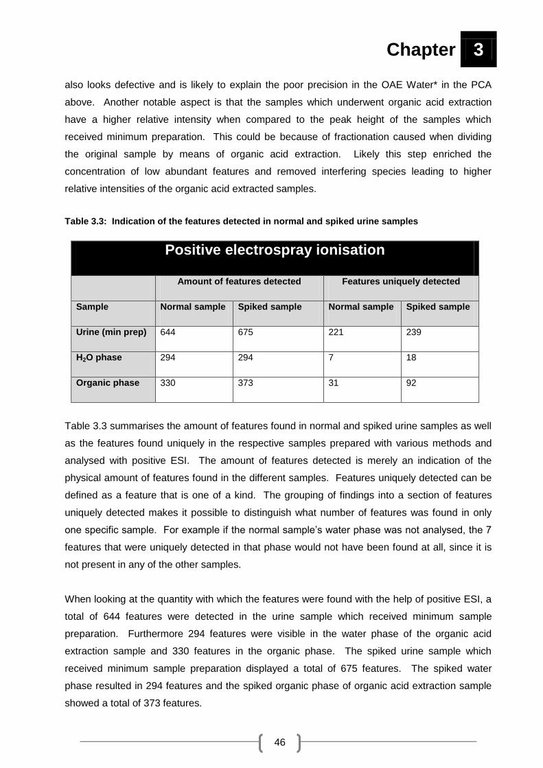
Chapter 3

46

also looks defective and is likely to explain the poor precision in the OAE Water* in the PCA

above. Another notable aspect is that the samples which underwent organic acid extraction

have a higher relative intensity when compared to the peak height of the samples which

received minimum preparation. This could be because of fractionation caused when dividing

the original sample by means of organic acid extraction. Likely this step enriched the

concentration of low abundant features and removed interfering species leading to higher

relative intensities of the organic acid extracted samples.

Table 3.3: Indication of the features detected in normal and spiked urine samples

Positive electrospray ionisation

Amount of features detected Features uniquely detected

Sample Normal sample Spiked sample Normal sample Spiked sample

Urine (min prep) 644 675 221 239

H2O phase 294 294 7 18

Organic phase 330 373 31 92

Table 3.3 summarises the amount of features found in normal and spiked urine samples as well

as the features found uniquely in the respective samples prepared with various methods and

analysed with positive ESI. The amount of features detected is merely an indication of the

physical amount of features found in the different samples. Features uniquely detected can be

defined as a feature that is one of a kind. The grouping of findings into a section of features

uniquely detected makes it possible to distinguish what number of features was found in only

one specific sample. For example if the normal sample’s water phase was not analysed, the 7

features that were uniquely detected in that phase would not have been found at all, since it is

not present in any of the other samples.

When looking at the quantity with which the features were found with the help of positive ESI, a

total of 644 features were detected in the urine sample which received minimum sample

preparation. Furthermore 294 features were visible in the water phase of the organic acid

extraction sample and 330 features in the organic phase. The spiked urine sample which

received minimum sample preparation displayed a total of 675 features. The spiked water

phase resulted in 294 features and the spiked organic phase of organic acid extraction sample

showed a total of 373 features.

Chapter 3

47

Evaluating the numbers given in Table 3.3 it is clear that samples that received minimum

sample preparation (labelled as urine) resulted in a larger amount of features. Since the urine

sample was fractioned into water- and organic phases using organic acid extraction, it is

expected that the sum of the features detected in the water and organic phase would be roughly

similar to that of the urine that received minimum sample preparation. Clearly this is not the

case and the exact reasons are unknown. One possibility may be that some features present in

both the water- and organic phase samples ended up being below the detection limit of the

instrument. This might also be the result of human error. Fractionation of urine samples with

the help of different methods increases the room for error which may result in the loss of some

features. On the other hand fractionation would reduce the amount of features that enter the

MS detector, ultimately reducing ion suppression.

When assessing the amount of features uniquely found in the normal and the spiked urine

samples a total of 221 features were only visible in the sample which received minimum sample

preparation. The word uniquely is used to emphasise that this features was only detected in

one of the sample extracts. Only 7 features were unique to the water phase of the organic acid

extraction sample and 31 features were only detected from the organic phase of the organic

acid extraction sample. Looking at the spiked urine sample analysed with positive ESI, 239

features were unique to the spiked urine sample which received minimum sample preparation.

A total of 18 features were uniquely found in the water phase of the spiked organic extraction

sample and 92 features were unique to the organic phase of the spiked organic extraction

sample.

Once again the samples which received minimum sample preparation provided a larger amount

of features for data analysis. A possible reason could be found in results obtained from

Newman et al., (2004) stating that the most accurate and precise method for analysis of organic

extracts proved to be a GC-MS. According to their findings the use of a LC-MS for organic acid

analysis leads to higher variability and the coefficient of variation were more than four times

higher. This confirms that an organic acid extracted sample preferably needs to be analysed

with a GC-MS (Newman et al., 2004).

Due to the ability of amino acids and organic acids which is commonly found in urine to carry a

negative charge, a decision was made to now analyse the same set of samples as used in the

cases of positive ESI with the help of negative ESI. Without changing anything except the

ionisation mode (and reference solution) the samples which received minimum sample

preparation and the samples that underwent organic acid analysis were analysed independently

in both ESI methods. The following PCA plots illustrate each sample set independently

Chapter 3

48

comparing the same sample analysed with different ESI methods. Positive ESI was used as

described in Sections 3.3 and 3.4. Negative ESI was used in the same manor (as positive ESI)

with the exception of the reference masses, which were 119.036320 (proton abstracted purine)

and 966.000725 (formate adduct of HP-921) m/z. This approach made it possible to verify if the

different sample preparation methods preferred one ionisation method more than the other.

Figure 3.9: Multivariate visualisation of spiked* and unspiked urine samples analysed with both

positive and negative ESI. From the left A illustrates the samples which received minimum sample

preparation, B represents the organic phase of samples which underwent organic acid extraction and C

symbolises the water phase of samples which underwent organic acid extraction

Figure 3.9.A summarises the findings observed when comparing urine samples (unspiked and

spiked) which received minimum preparation and were analysed with both positive and negative

ESI. On the left hand side of the figure the samples analysed with negative ESI is visible. The

solid dots represent the unspiked urine samples and the diamonds the spiked urine samples.

On the right hand side the samples analysed with positive ESI can be found. The squares

found on top represent the spiked urine samples and the circles on the bottom represent the

unspiked urine samples. In PC1 of this figure it’s visible that the samples analysed with

negative (left side) and positive (right side) ESI separated excellent. PC2 of this figure shows

that the spiked urine samples (top) and unspiked urine samples (bottom) also separates very

good. Thus separating urine samples analysed with positive and negative ESI as well as

separating spiked and unspiked urine samples is no problem when the sample received

minimum sample preparation.

In Figure 3.9.B the organic phase of urine samples which underwent organic acid extraction can

be seen when analysed with both positive and negative ESI methods. In the top left hand

corner the spiked urine samples analysed with negative ESI represented by diamonds can be

A B C

Chapter 3

49

seen. The solid dots spread across the left side represent the unspiked negatively analysed

urine samples. The squares in the top on the right hand side represent the spiked urine

samples analysed using positive ESI. Lastly the circles represent the positively analysed

unspiked urine samples. This Figure shows good repeatability and separation when looking at

the spiked urine samples (top corners). The unspiked urine samples are a good illustration of

poor repeatability and separation, since they are spread across the picture.

The water phase of the urine samples prepared using organic acid extraction and analysed with

positive and negative ESI are illustrated in Figure 3.9.C. The left hand side shows the samples

analysed with negative ESI. The solid dots represent the unspiked urine samples and the

diamonds represent the spiked urine samples. On the right hand side the samples analysed

using positive ESI can be seen. The circles to the top represent the unspiked urine samples

and the squares represent the spiked urine samples. One clear conclusion concerning this

figure is the fact that positive (right side) and negative (left side) ESI can clearly be separated

from one another. The separation of the spiked and unspiked urine samples within an

ionisation class is of poor quality.

Looking at all the figures it can be concluded that the urine samples which received the

minimum preparation provided better results and less variation regardless of the ionisation

method used. This indicates that organic acid extraction as a preparation method for urine

samples shouldn’t be used as a primary preparation method for untargeted LC-MS analysis.

Chapter 3

50

3.8 STANDARDISED LC-Q-TOF METHOD FOR POSITIVE ESI

After evaluation of a number of factors discussed in this chapter, the following standardised

method using positive ESI was used to investigate respiratory chain deficiencies in urine

samples utilising an untargeted LC-MS metabolomics approach (Figure 3.10).

Figure 3.10: Workflow followed for sample analysis using positive ESI. The following steps were

followed as the workflow for positive ESI: a first round of urine preparation; freezing; a drying step; a

second round of urine preparation; LC-Q-TOF analysis; data extraction steps, statistical manipulations

and ultimately result interpretation.

Received urine samples were stored at -80˚C before any analysis was conducted. By using the

creatinine values of each sample (which was predetermined by the Jaffe method) the amount of

urine needed to ensure a creatinine value of 0.25 μmol per sample was determined by means of

a creatinine calculator.

The first urine preparation step was done just after the urine underwent overnight thawing (at

4˚C). This step included the addition of an individually determined volume of urine along with

10 μl of internal standard (nor-leucine, 2-acetamidophenol and caffeine) and 20 μl of acetonitrile

Chapter 3

51

(ACN) in a micro tube. Once this was completed the samples were frozen at -80°C overnight.

The frozen sample mixture was dried by using a speed vac to compensate for varying sample

volumes.

Next the samples were prepared for LC-Q-TOF analysis by implementing a second step of urine

preparation. As soon as the dried urine samples received 100 µl of mobile phase (100 µl water)

a waiting period of 30 minutes was allowed to ensure that the dried sample would fully dissolve.

There after the samples were vortexed for 10 seconds to ensure complete re-suspension of the

dried urine sample. Next the samples were centrifuged in separate micro tubes at 25 055 X g

for 10 minutes at 4˚C before further analysis. After the mixtures were thoroughly mixed a

volume of 70 μl of the clear supernatant was transferred into LC vials fitted with pointed inserts.

The LC-Q-TOF method followed comprised of an LC connected to a Q-TOF (described in

Section 3.3) switched to positive ESI. A reverse phase C18 column was used, using water (1L)

and acetonitrile (1L) containing 0.1% formic acid as mobile phase modifier. A total run time of

50 minutes (42 minute gradient and 8 minute post run) per sample was used for

chromatographic separation. The chromatographic gradient started at 0% solvent B for 5

minutes, where after the gradient was increased to 35% solvent B over a period of 25 minutes.

Next the gradient was increased to 70% solvent B at time point 35 minutes and 100% solvent B

at 36 minutes. The gradient was kept at 100% solvent B for 3 minutes and then decreased to

0% over 3 minutes. Once the run was completed a post run of 8 minutes was allowed to ensure

equilibration of the column. A total of 61 samples along with quality control samples were

divided into two batches that were analysed with the LC-Q-TOF.

MFE and FbI were used to extract and manipulate the data, followed by binning and alignment

in MPP (Section 3.6). The HMDB was used to assign annotated names to features whenever

possible. Lastly the extracted data underwent a set of statistical manipulations using Microsoft

excel and Metabo-analyst. All in all this led to a series of results to be interpreted.

52

CHAPTER 4:

Untargeted negative ESI

LC-MS assay

Chapter 4

53

4.1 INTRODUCTION

Untargeted metabolomic strategies rely largely on the ability to detect thousands of metabolites

from a biological sample. Keeping in mind that the human metabolome consist of numerous

compound classes it is vital to use different techniques in an attempt to cover a vast majority of

metabolome. By diversifying the method at hand one can take advantage of more than one

retention process and ionisation technique, resulting in a larger group of detected metabolites

(Scalbert et al., 2009).

In this chapter different experimental strategies were followed when using negative electrospray

ionisation (ESI). The primary thing to do was to compare different sets of mobile phase

modifiers. The modifiers of choice included: 17 mM acetic acid; 5 mM acetic acid; 5 mM

ammonium acetate pH 4.5 and 5 mM ammonium acetate pH 7.0. The main purpose for altering

mobile phase modifiers was to find a modifier that wound fit negative ESI methods in the same

way formic acid fits positive ESI methods. Next a hydrophilic interaction chromatography

(HILIC) column was used for analysis in an attempt to retain polar molecules, because small

polar compounds such as amino acids and organic acids co-elute very early from a reverse

phase column (Chen et al., 2009). Furthermore negative ESI was found to be sufficient since

these compounds that are likely to be retained longer on a HILIC column, tend to carry a

negative charge.

4.2 REAGENTS AND BUFFERS

4.2.1 Q-TOF reagents

Spectrometry grade acetonitrile (Honeywell Burdic and Jackson, cat # BJ015CS) and water

(Honeywell Burdic and Jackson, cat # BJ365CS) were purchased from Anatech and used as

mobile phase solvents. Acetic acid (Sigma-Aldrich, cat # 49199) and ammonium acetate

(Sigma-Aldrich, cat # 17836) were used as mobile phase modifiers.

4.2.2 Standard preparation

A standard mixture consisting of adenosine (Sigma-Aldrich, cat # 58617), nor-leucine (Sigma-

Aldrich, cat # 74560) and uracil (Sigma-Aldrich, cat # 66228) with an end concentration of 1 000

Chapter 4

54

ppm was prepared to be used as a known mixture when optimising the preferred conditions for

a HILIC column.

4.2.3 Internal standard preparation

Thirty milligrams of 3-phenylbutyric acid (Sigma-Aldrich, cat # 78243) were weighed and

dissolved with MilliQ H2O in a falcon tube. Nor-leucine and 2-acetamidophenol were also used

as an internal standard when performing negative ESI and prepared according to the

procedures described in Section 3.2.4. A mixture of the three standards was prepared with an

end concentration of 1 000 ppm. This mixture was stored at 4ºC and used as internal standard

for all experiments conducted with negative ESI.

4.3 INSTRUMENTATION

4.3.1. LC-QQQ

A 1200 series LC system (Agilent Technologies, Santa Clara, CA, USA) coupled to an Agilent

6410 QQQ was used to optimise the HILIC chromatographic conditions. The following

components were included in the LC system: a Micro Vacuum Degasser (G1379B); Binary

pump SL (G1312B); Preparative Auto sampler HiP-ALS SL (G1367C); Thermostat ALS

(G1330B) and Thermostatted Column Compartment SL (G1316B). The auto sampler’s

temperature was set to 4°C to ensure that the samples were kept cool.

Multiple-reaction monitoring (MRM) on a QQQ was used to standardise the chromatographic

separation conditions due to the high level of sensitivity which is presented with this method

(more detail will follow in Section 4.7.2.2). MRMs were optimised for all compounds using

Agilent Technologies Optimizer software. The optimal MRM configuration settings are shown in

Table 4.1.

Chapter 4

55

Table 4.1: MRM conditions used to detect uracil, nor-leucine and adenosine

Compounds Precursor Ion

(m/z)

Fragmentor

voltage (V)

Product Ion

(m/z)

Collision

Energy (eV)

Uracil 113 80 70 15

Nor-leucine 132.1 77 86.2 8

Adenosine 268.1 94 136.1 16

The MS conditions included: Electrospray ionisation as ion source; a drying gas flow of 8 L/min;

nebuliser pressure of 30 psi and a drying gas temperature of 280°C. Agilent’s Mass Hunter

Acquisition software was used as an operating system.

4.3.2. LC-Q-TOF

At 1290 series LC system (Agilent Technologies, Santa Clara, CA, USA) coupled to a 6540 Q-

TOF mass analyser from Agilent was used for sample analysis as described in Chapter 3

(Section 3.3.1).

The duel ESI source was set for negative electrospray ionisation. The drying gas temperature

was set at 280°C, using a drying gas flow of 8 L/min and nebuliser pressure of 30 psi. The

acquisition rate was 1.5 spectra per sec and a stored mass range of 50 to 1 000 m/z. Both

centroid and profile data were stored. The instrument mode was set to extended dynamic

range (2 GHz). The Agilent Q-TOF reference solution containing purine (119.036320) and an

acetate adduct (980.016375) were constantly infused as accurate mass reference. When

starting a new set of analysis the instrument was calibrated with Agilent ESI-L low concentration

tuning mix (G1969-8500). Agilent’s Mass Hunter Acquisition software was used as operating

system during analysis (Lindeque et al., 2013).

The LC-Q-TOF was used in this part of the study, to experiment with different mobile phase

modifiers. A Q-TOF can be regarded as the perfect system to use when doing untargeted

studies because of its ability to detect hundreds to thousands of metabolites with great accuracy

(Scalbert et al., 2009).

Chapter 4

56

4.4 CHROMATOGRAPHIC SEPARATION

4.4.1 Reverse phase chromatography

Chromatography was performed with an Agilent ZORBAX SB-Aq reverse phase (Chemetrix,

830990-914) C18 column (3.5 μm, 2.1 X 150 mm). A total of four different sets of mobile

phases were evaluated for negative ionisation. The first mobile phase combination contained

17 mM acetic acid in 1L water (solvent A) and 17 mM acetic acid in 1L acetonitrile (solvent B).

The second mobile phase combination contained 5 mM acetic acid in 1L water (solvent A) and

5 mM acetic acid in 1L acetonitrile (solvent B). Thirdly a set of mobile phases containing 5 mM

ammonium acetate in 1L water (solvent A) with a pH of 4.5 and 5 mM ammonium acetate in 1L

acetonitrile (solvent B) with a pH of 4.5 was used. The fourth set of mobile phases had a pH of

7.0 and contained 5 mM ammonium acetate in 1L water (solvent A) and 5 mM ammonium

acetate in 1L acetonitrile (solvent B). The same chromatography conditions as described in

Section 3.4 were used in this case.

4.4.2 Hydrophilic interaction chromatography

An Agilent ZORBAX RRHD HILIC plus (Chemetrix, 959759-901) column (1.8 μm, 2.1 X 150

mm) fitted with a Phenomenex guard column (AFO-8497) was used. Solvent A of the mobile

phase consisted of 5 mM acetic acid in water and solvent B contained 5 mM acetic acid in

acetonitrile. After mobile phase preparation both solvents were degassed for 5 minutes in an

ultrasonic bath.

A chromatographic gradient with a run time of 25 minutes and a post run time of 10 minutes per

sample was used. The gradient began at 90% solvent B and maintained for 2.5 minutes, after

which the gradient was decreased to 50% solvent B at the 10 minute mark. Solvent B was kept

at 50% for 5 minutes where after the gradient was raised back to 90% solvent B at time 20

minutes. The gradient was kept at 90% solvent B for 5 minutes until the run was complete. A

column temperature of 35°C and a flow rate of 0.25 ml/min were used when performing the

analysis. A volume of 5 μl per sample was injected into the system during analysis.

Chapter 4

57

4.5 DATA EXTRACTION

LC–MS data were extracted and manipulated with the help of Agilent’s Mass Hunter Qualitative

software and Mass Profiler Professional software using MFE and FbI algorithms. Where

possible the HMDB was used to annotate compounds. Full detail of the process can be viewed

in Chapter 3 (Section 3.6).

4.6 TUNING AND CALIBRATION

Untargeted metabolomic experiments are largely based on accurate mass determination of

compounds. The precision and accuracy achieved with a Q-TOF depends on a variety of

technical parameters. Typically one would calibrate and tune the Q-TOF system with a mixture

of compounds with known masses to ensure the best possible results (Mihaleva et al., 2008).

As part of standard procedure the instrument was auto-tuned every six months or according to

maintenance protocols using Agilent technologies ESI-L low concentration tuning mix (G1969-

8500). Tuning is implemented to adjust the quadruple parameters to achieve maximum signal

intensity while maintaining acceptable resolution.

Calibration is the process where accurate masses based on known masses of standard

compounds are assigned to Q-TOF mass axis. Calibration was done before the analysis of a

batch of samples using the ESI-L low concentration tuning mix (G1969-8500). Calibration

results in a calibration curve showing the time-to-flight to mass fit of the polynomial correction,

across the full mass range. This calibration curve is guided by the 10 masses found in the

tuning mix (which differ from the reference solution). Once calibration is completed a ppm error

will appear. Ideally one would aim for a mass error of less than 1 ppm for all tune ions. If any

mass errors are greater than 3 ppm it is advised to repeat the calibration. All in all calibration

ensures mass accuracy of the instrument. It also makes it possible to perform mass axis

correction once the samples are analysed (AGILENT-TECHNOLOGIES, 2012).

Chapter 4

58

4.7 METHOD DEVELOPMENT

When using electrospray ionisation (ESI) as an ionisation method the ability to analyse both

high and low molecular weight compounds exists. Nearly all compounds that can form an ion in

solution can be analysed with ESI. Focusing on negative ESI the most common base peaks

are [M-H]-. Other fragments and adducts likely to form in negative ion mode include: [M+Cl]-;

[M-H-CO2]-; [M-H+HCOONa]-; [M-H-HCOOH]- etc. (Holčapek et al., 2010).

A combined display of the steps followed in negative ESI can be seen in Figure 4.1. Different

mobile phase modifiers and chromatography on a HILIC column were evaluated in an attempt

to find a suitable untargeted LC-MS assay using negative electrospray ionisation.

Figure 4.1: Summary of steps to follow for experimentation using negative ESI. The two steps

used included experimentation with different mobile phase modifiers and chromatography

experimentation on a HILIC column.

4.7.1 Different mobile phase modifiers

The use of 0.1% formic acid as mobile phase modifier has become common knowledge when

using positive electrospray ionisation. However when it comes to the selection of an additive in

negative ion mode, the choice tends to be more complicated. Since additives can improve

Chapter 4

59

ionisation efficiency for different metabolites in negative ESI the pursuit for the most suitable

modifier among acetic acid and ammonium acetate, which is generally used for negative ESI,

arose. As part of the experimentation process for this untargeted urine metabolomics study the

effect of separately adding 17 mM acetic acid, 5 mM acetic acid, 5 mM ammonium acetate with

a pH of 4.5 and 5 mM ammonium acetate with a pH of 7.0 to both the water and acetonitrile

mobile phase solvents, were investigated.

While researching the appropriate mobile phase modifiers used in negative ESI a few

possibilities surfaced pinpointing acetic acid, ammonium acetate and ammonium formate as the

most popular choices. The choice to keep the mobile phases enriched with acetic acid and

ammonium acetate at the same concentration (of 5 mM) was made to rule out the possibility

that differences in ionisation efficiency are related to the concentration of the modifier. By using

a high additive concentration it is likely to decrease ionic strength and increase the signal-to-

noise ratio in negative ion mode (Wu et al., 2004). Furthermore they reported that weaker acids

like acetic acid enhanced negative ESI responses in concentrations < 10 mM. Thus it can

assume that moderate concentrations of protons are essential to facilitate negative ESI. Yanes

et al., (2011) also advised against a high concentration of mobile phase modifier since

precipitation of the modifier occurs when the acetonitrile increased above 50%.

By keeping a constant pH in both mobile phases (H2O and ACN) a higher intensity could be

ensured from the buffer while using a lower salt concentration. Since it is reasonable to assume

that the addition of a base would facilitate the deprotonation of analytes in negative ion mode,

working at a lower pH would be beneficial for negative ESI analysis. Furthermore it was also

reported that a solution with a pH of 4 to 4.5 was optimal in negative ESI. It is recommended

that the difference between the pH of the LC solvent and the pKa of the analyte should be

above 2 units by which the analyte exists fully ionised or neutral (Zhang et al., 2012).


Two urine samples labelled as control A (creatinine concentration of 9.8 mmol/l) and control B

(creatinine concentration of 9.6 mmol/l) were collected and stored at -80˚C before being

analysed. After overnight thawing (at 4˚C) the samples where centrifuged at 25055 X g for 15

minutes at 4˚C in separate micro tubes. Next, five individual mixtures of control A and B were

prepared, resulting in an end volume of 100 μl and an IS sample concentration of 1 000 ppm.

Control A consisted of: 10 μl IS (described in Section 4.2.3), 25.5 μl urine and 64.5 μl of MilliQ

H2O. Control B contained: 10 μl IS (described in section 4.2.3), 26.05 μl urine and 63.95 μl of

Chapter 4

60

MilliQ H2O (to compensate for varying urine volumes a creatinine content of 0.25 µmole was

determined for all of the samples). Ten LC vials with tapered inserts containing the prepared

samples were analysed with the Q-TOF system using negative ESI according to the procedures

mentioned in Sections 4.3.2 and 4.4.1. This step of the experimentation was done using a

reverse phase column since it can be regarded as a successfully working model and to ensure

that only one variable at a time is changed. After sample analysis the data were extracted and

analysed according to the process described in Section 4.5. After data analysis was completed

statistical manipulations with the help of Microsoft Excel and Metabo-analyst were performed.


An educated decision regarding the most suitable mobile phase modifier for negative ESI could

not be made entirely on the visual results obtained in the form of chromatograms, thus Table

4.2 was compiled in an attempt to persuade the decision towards one additive.

Table 4.2: Data manipulations

Statistical evaluations Acetic acid

(17 mM)

Acetic acid

(5 mM)

Ammonium

acetate (pH 4.5)

Ammonium

acetate (pH 7.0)

All detected features 6946 1073 424 535

Features kept after zero filter 1437 566 307 261

Features kept after CV filter 1002 531 297 223

Features fully present in group A 772 515 220 216

Features fully present in group B 711 502 255 161

Minimum average CV value 24.90% 8.92% 9.91% 16.23%

Maximum average CV value 84.31% 39.30% 37.68% 38.78%

Dynamic range (min) 24121.5 172.2 12557.5 12557.5

Dynamic range (max) 35422678.2 33372594 5812256 7493116

Statistical significantly features 422 327 142 34

Table 4.2 is a summary of data processing and manipulations executed on the data supplied

after extraction of the samples analysed with a LC-Q-TOF. In an attempt to select an additive

best fit for negative ESI the following aspects were evaluated: coverage; accuracy; precision;

coefficient of variance; dynamic range and number of features that differed significantly between

the two groups. Factors like running time, amount of mobile phase used and price per sample

Chapter 4

61

which is usually of importance when making decisions like this resulted in the same answer for

all four options.

The amount of features found in the data matrix can be seen in the first row of Table 4.2. Here

it is shown that the most features were extracted from the sample analysed with 17 mM acetic

acid added to the mobile phase solvents. A total of 6 946 features were found when using 17

mM acetic acid, the least amount of features namely 424, were found when using 5 mM

ammonium acetate with a pH of 4.5.

Zero filtering (removal of uncommon variables) was implemented to remove features that

weren’t present in all groups (Lindeque et al., 2013). The features were filtered by removing

features that were not fully present in at least one group (of 5 replicates). The remaining

features were used for PCA compiling. The amount of features kept when using 17 mM acetic

acid as modifier ads up to 1 437. When using the 5 mM acetic acid modifier, 566 features were

kept while 307 and 261 features remained when ammonium acetate pH 4.5 and pH 7.0 were

used respectively.

The second filter applied to the data was a CV filter with a cut-off point of 50%. Features with a

CV value of less than 50% in any of the two groups were kept as that meant that compound

degradation was minimal and the instrument capable to analyse them precisely. Seeing that

the groups consist of 5 replicates, there should be as little variance between the replicates as

possible. After this step was implemented, 17 mM acetic acid still presented the most features

namely 1 002 and 5 mM ammonium acetate with a pH of 7.0 presented the least amount of

features namely 223. The features fully present in group A and B is a summary of the features

which were found in all of the five samples without any absences, thus can also be seen as an

indication of how repeatable a feature was found.

In order to determine the minimum (and maximum) average CV value, CV values of the two

experimental groups were calculated followed by a sorting step where the minimum (or

maximum) value between the two groups for each feature was determined. Once all of the

features minimum (or maximum) CV value was determined the average of the data was

calculated. The 5 mM acetic acid mobile phase modifier supplied the lowest CV value of 8.9%

among all the data sets. The mobile phase modifier consisting of 17 mM acetic acid supplied

the highest CV average of 84.3%.

The dynamic range rows (minimum and maximum) give an indication at what

concentration/abundance the features were found in the various mobile phases. This can be

Chapter 4

62

regarded as a display of how ionisation was influenced. The modifier consisting of 17 mM

acetic acid displayed the highest value. The mobile phase consisting of 5 mM acetic acid used

as modifier showed the lowest value among the datasets, stating that this modifier is able to

detect features at low concentrations.

In order for a feature to be selected for further analysis, the feature has to adhere to certain

parameters. Ultimately the parameters aim to keep features that are statistical significant.

Student’s t-test was used to determine if there is a statistical significant between the

experimental group’s means by determining a P-value. A P-value is considered as statistically

significant whenever the value is less than as 0.05. The effect size (ES) was also determined to

show whether the statistical difference was also practical. This is expressed as a d-value.

Usually log-transformed data with a d-value of 0.8 can be classified as practically significant

(Ellis and Steyn, 2003). In this case all the features with a t-test P-value < 0.05 and an effect

size d-value > 0.8 were used to select features for PCA compilation. The number of features

obtained with feature selection is also an important indicator of which modifier is more suited.

The reason for this is that with the test design (where two groups exist that both consist of 5

replicates each) the intragroup variance (between the replicates) should be lower than the

intergroup variance (variance between the two groups). Because of this, a univariate test like t-

test would find significant differences between the groups even if the means of the metabolites

do not differ much.

Chapter 4

63

Figure 4.2: PCA plots based on features found after basic data manipulations. The PCAs display

separation between two groups using different mobile phase modifiers. Figure A represents 17 mM

acetic acid, Figure B represents 5 mM acetic acid, Figure C represents 5 mM ammonium acetate with a

pH of 4.5 and Figure D represents 5 mM ammonium acetate with a pH of 7.0.

Figure 4.2 represents the principal component analysis done on the data analysed with the four

mobile phase modifiers of choice. In all of the cases two different groups were analysed,

namely group A (Δ red) and group B (+ green). In Figure 4.2.A samples analysed with a mobile

phase containing 17 mM acetic acid can be seen. Next in Figure 4.2.B the samples analysed

with an additive of 5 mM acetic acid are displayed in the PCA score plot. The samples

D C

B A

Chapter 4

64

analysed with the 5 mM ammonium acetate (pH 4.5) modifier are visible in Figure 4.2.C. Figure

4.2.D shows the PCA plot when using 5 mM ammonium acetate (pH 7.0) as modifier.

Evaluating the images the same trend seems to follow for the same mobile phase modifiers. In

both acetic acid cases (17 mM and 5 mM) group B clusters to the left side of the figure and

group A to the top side. In the PCA score plots representing ammonium acetate example one of

the groups in each figure clusters close together, while the opposite group appears to be

stretched out amongst the figure.

From the four scenarios the ammonium acetate (pH 7.0) can be classified as the worst modifier

to use in negative ESI, since no separation between the two experimental groups is visible. The

best clustering within a group can be seen when looking at ammonium acetate (pH 4.5). If the

one sample found in group A in this figure was aligned with the rest of the samples in its group,

almost identical distribution of the samples would be present, ultimately supporting good

repeatability of the samples. The acetic acid examples are likely to be ranked as the figures

with the best separation between the two groups, considering that their relationship between

intergroup and intragroup variation exceeds that of the ammonium acetate example.

The most prominent conclusion that can be drawn from by Table 4.2 is that 5 mM ammonium

acetate with a pH of 7.0 should not be used as mobile phase modifier when doing untargeted

analysis in negative ESI. It was reported that a pH of 7 should be used when doing negative

ionisation on a C18 column using 1 mM ammonium fluoride as modifier (Yanes et al., 2011). In

consideration of the next step of the experimentation process, a modifier that would be

compatible with a HILIC column needed to be selected. For a HILIC column to operate at its

best and to prolong the column lifetime is it recommended that the pH of the mobile phase

should range between 2 to 6. Thus 5 mM ammonium acetate (pH 7.0) was ruled out as

modifier for negative ESI. The mobile phases using 17 mM acetic acid were also ruled out as a

choice for a modifier due to its insufficient pH value of 6.6.

Now the choice regarding the best mobile phase modifier needed to be made between 5 mM

acetic acid and 5 mM ammonium acetate (pH 4.5). Looking back at Table 4.2 and narrowing

the focus to the 5 mM acetic acid and 5 mM ammonium acetate (pH 4.5) columns, the acetic

acid additive resulted in a more abundant data matrix exceeding the quantity of what was found

with 5 mM ammonium acetate. Looking at the quality of the supplied data it would seem that

the ammonium acetate additive is the better option. This can be derived from the amount of

features found in both cases and comparing this finding to the number of features used for the

first PCA. The amount of features found with acetic acid is about cut in half from 1 073 to 566.

Chapter 4

65

Ammonium acetate on the other hand loses just over a 100 features when reduced from 424 to

307. It can be speculated that ammonium acetate found features in al ten samples in a more

reproducible fashion.

The strengths of 5 mM acetic acid as mobile phase modifier included: 1) Acetic acid ensured a

large data matrix; 2) CV values indicated that the results are reproducible; 3) Good separation

between the experimental groups are visible in the PCA’s supplied; 4) Acetic acid (pH 3.62 in

water solvent and pH 4.1 in acetonitrile solvent) can function between the appropriate pH values

needed for a HILIC column; 5) Reasonable buffering capacity occurs resulting in good

chromatographic separation; 6) The additive is stable in different mobile phase solvents and

requires minimum preparation. Thus 5 mM acetic acid can be regarded as a sufficient mobile

phase modifier for negative ESI.

4.7.2 Hydrophilic interaction chromatography (HILIC)

Even though reverse phase chromatography is the most widely adopted retention mechanism

for the majority of separations it lacks the ability to effectively retain small polar analytes. As an

alternative, hydrophilic interaction chromatography is rapidly becoming the preferred technique

when analysing polar and/or basic solutes (Buszewski and Noga, 2012). Due to the limited

interaction mechanisms supplied by reverse phase chromatography it was decided to use a

complementary LC column (in this case a HILIC column) as part of the experimentation process

in an attempt to retain/separate polar compounds better and acquire better data for these small

polar compounds. This is especially important since RCDs normally result in an accumulation

of organic acids and related polar compounds.

Reverse phase columns make use of an apolar stationary phase and a polar mobile phase. In

this technique the most polar compounds will elute first and the most apolar compounds at the

end of the chromatographic run. Normal phase columns use a polar stationary phase and an

apolar mobile phase. The elution process will progress from the least to the most polar

compounds. HILIC columns can be seen as a combination of reverse phase and normal phase

columns. HILIC columns are distinguished by a polar stationary phase and an aqueous polar

organic solvent mobile phase. Elution of compounds will follow a similar pattern like in the case

of normal phase columns with exception of better solubility of hydrophilic compounds

(Dejaegher and Vander Heyden, 2010, Gama et al., 2012).

The functioning of a HILIC column is based on the mechanism that polar groups attach to the

stationary phase of the column and attract water molecules to form an aqueous layer over the

Chapter 4

66

surface of the stationary phase. A polar analyte which is present in the mobile phase will

undergo partitioning between the two liquid phases. Due to the fact that polar solutes have a

higher affinity for the aqueous layer, increased interaction of the solute with the aqueous layer

will take place, leading to increased retention. Hydrogen bonding participates in this process,

possibly as a driving force in the partitioning, while electrostatic interactions contribute to the

retention mechanism to a varying degree, depending on the nature of the stationary phase and

mobile phase (Buszewski and Noga, 2012, Gama et al., 2012).


Standard mixture analysis:

A 10 ppm mixture of three standard compounds (nor-leucine, uracil and adenosine) was

prepared by diluting the standard prepared in Section 4.2.2. These compounds have no or little

retention on a reverse phase column and were thus selected to standardise HILIC conditions.

These samples were analysed with an Agilent QQQ using positive ESI according to the details

mentioned in Sections 4.3.1 and 4.4.2. After MRMs were completed Mass Hunter Qual

software was used to examine the chromatographic results.

Urine analysis:

Two urine samples (A and B) were prepared by centrifuging 1 ml of the thawed urine sample at

25055 X g for 15 minutes at 4˚C in separate micro tubes. After this process five replicates of

sample A (10 μl IS, 25.5 μl urine and 64.5μl of MilliQ H2O) and sample B (10 μl IS, 26.05 μl

urine and 63.95 μl of MilliQ H2O) were prepared (to compensate for varying urine volumes a

creatinine content of 0.25 µmole was used in all of the samples). These samples were

transferred to LC vials with tapered inserts ready to be analysed with the LC-Q-TOF system in

negative ion mode using the conditions and specifications described in Sections 4.3.1 and

4.4.2. Once the samples were analysed the data were extracted following the process

described in Section 4.5. The process was ended with statistical manipulations in Metabo-

analyst.

Chapter 4

67


Since it is difficult to maintain control over the findings in a sample when using an untargeted

approach, this part of the standardisation process started with a targeted analysis. It was

necessary to monitor a few single compounds (instead of an untargeted assay) to get a method

in place for HILIC analysis (since prior experience with HILIC columns was limited). This

targeted analysis included MRMs of uracil, adenosine and nor-leucine. When doing MRM

analysis a high level of sensitivity can be achieved due to the fact that information regarding a

precursor ion, a product ion and retention time is available. This made it easier to vary

chromatographic conditions because of the ability to cross check findings with known

references.

The different experimental conditions that were evaluated included: 1) Percentage of H2O

(solvent A) at time 0 minutes of the chromatographic separation; 2) Flow rate; 3) Repeatability;

4) Column equilibration; 5) Seeing if the process could be repeated in an untargeted fashion on

a LC-Q-TOF.

Water can be regarded as very important when doing HILIC separations, but to what extent can

the chromatographic gradient be pushed before no retention of the compounds occurs?

Amongst different sources the percentage of water to be used as mobile phase can range from

5% to 40%. It is advised that a minimum of 2% should always be present to ensure the

formation of the aqueous layer which plays an important role in the HILIC separation process

(Gama et al., 2012). Six different combinations of starting points for mobile phase A and B were

assessed when analysing the three standards (described in Section 4.7.2.1) in six different

runs. In all of the cases the gradients lowest point was 60% H2O and 40% acetonitrile at the 10

minute mark, after which the gradient was increased back to the starting condition. The first

mixture started at 10% H2O and 90% acetonitrile; secondly 9% H2O and 91% acetonitrile was

tested; thirdly 8% H2O and 92% acetonitrile was used; fourthly the ratio changed to 7% H20 and

93% acetonitrile, fifthly 6% H2O and 94% acetonitrile was used and the last condition ended at

5% H2O and 95% acetonitrile. The result was simple and indicated that an increase in the

organic mobile phase extended the compounds retention time on the column. Thus a decrease

in the water mobile phase allowed better retention of the compounds. The following table

indicating the retention time at which the compounds were found, can elaborate on this

observation.

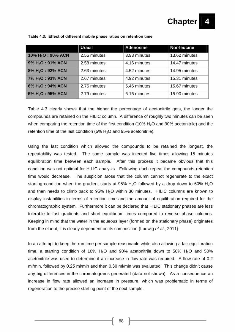
Chapter 4

68

Table 4.3: Effect of different mobile phase ratios on retention time

Uracil Adenosine Nor-leucine

10% H2O : 90% ACN 2.56 minutes 3.93 minutes 13.62 minutes






Table 4.3 clearly shows that the higher the percentage of acetonitrile gets, the longer the

compounds are retained on the HILIC column. A difference of roughly two minutes can be seen

when comparing the retention time of the first condition (10% H2O and 90% acetonitrile) and the

retention time of the last condition (5% H2O and 95% acetonitrile).

Using the last condition which allowed the compounds to be retained the longest, the

repeatability was tested. The same sample was injected five times allowing 15 minutes

equilibration time between each sample. After this process it became obvious that this

condition was not optimal for HILIC analysis. Following each repeat the compounds retention

time would decrease. The suspicion arose that the column cannot regenerate to the exact

starting condition when the gradient starts at 95% H2O followed by a drop down to 60% H2O

and then needs to climb back to 95% H2O within 30 minutes. HILIC columns are known to

display instabilities in terms of retention time and the amount of equilibration required for the

chromatographic system. Furthermore it can be declared that HILIC stationary phases are less

tolerable to fast gradients and short equilibrium times compared to reverse phase columns.

Keeping in mind that the water in the aqueous layer (formed on the stationary phase) originates

from the eluent, it is clearly dependent on its composition (Ludwig et al., 2011).

In an attempt to keep the run time per sample reasonable while also allowing a fair equilibration

time, a starting condition of 10% H2O and 90% acetonitrile down to 50% H2O and 50%

acetonitrile was used to determine if an increase in flow rate was required. A flow rate of 0.2

ml/min, followed by 0.25 ml/min and then 0.30 ml/min was evaluated. This change didn’t cause

any big differences in the chromatograms generated (data not shown). As a consequence an

increase in flow rate allowed an increase in pressure, which was problematic in terms of

regeneration to the precise starting point of the next sample.

Chapter 4

69

Going back to repeatability a gradient with a maximum of 90% acetonitrile and minimum of 50%

along with a flow rate of 0.25 ml/min and a total run time of 25 minutes per sample followed by a

10 minute equilibrium step after each sample, was used to verify if the HILIC method was

satisfactory. Four samples were injected after one another to evaluate if a shift in retention time

was present. Figure 4.3, 4.4 and 4.5 displays the result obtained from the first and then the last

sample injected.

Figure 4.3: Chromatographic illustration of uracil. Chromatograms illustrating uracil found with MRM

at the beginning and the end of a batch.

Chapter 4

70

Figure 4.4: Chromatographic illustration of adenosine. Chromatograms found when doing MRM of

adenosine in two different samples.

Figure 4.5: Chromatographic illustration of nor-leucine. Chromatograms of nor-leucine at two

different time intervals found using MRM.

Chapter 4

71

In Figure 4.3 the retention time (RT) of uracil is visible in two different samples (at the beginning

and the end of a run). In the first sample a RT of 1.988 minutes was reported followed by a RT

of 1.997 minutes in the last sample. Figure 4.4 displays the retention time of adenosine found

when doing MRMs. At the beginning a RT of 3.163 minutes was observed and in the end this

RT shifted to 3.154 minutes. Nor-leucine was found at a RT of 9.445 minutes in the first sample

and in the last sample the RT displayed a time of 9.430 minutes as seen in Figure 4.5.

This result indicates that a negligible small shift in retention time takes place throughout a batch

of samples. Considering this, it is possible to trust the HILIC method being used in this study.

Now that a repeatable and reliable HILIC method was developed the focus shifted from three

compounds to urine samples. Urine contains a lot of water soluble metabolites which contains

important characteristics and information for experiments (Chen et al., 2009). As urine is

predominantly aqueous, a significant proportion of the content is likely to be highly polar and

would typically be unretained on reverse phase columns and thus would not contribute to the

data obtained (Cubbon et al., 2007). As a result HILIC mechanisms would be a perfect

technique to use in combination with reverse phase mechanisms to analyse urine samples in an

untargeted manor.

Looking back at liquid chromatography methods used in previous studies at the North-West

University’s Metabonomics platform, the results indicated that reverse phase chromatography in

positive ion mode were satisfactory. These studies potentially missed out on the opportunity of

finding highly polar metabolites such as sugars, amino acids, nucleic acids and organic acids,

since they are not retained by conventional reverse phase LC columns. Furthermore it would

be possible for these compounds to be negatively charged, thus making them perfect targets for

negative ESI.

Saric et al., (2012) reported that chromatograms obtained with negative ESI were richer in

terms of polar compounds (organic acids, AMP, amino acids). They also found that half of the

identified compounds were not properly retained by a C18 column. Furthermore negative ESI

found more small polar metabolites than positive ESI. Nevertheless they confirmed that both

ionisation modes contributed to unique metabolites.

Remembering that polar compounds such as organic- and amino acids are likely to carry a

negative charge, along with the fact that polar compounds elute fast from a reverse phase

column it was deemed fit to do analysis on a HILIC column in negative ion mode. Ultimately it is

Chapter 4

72

suggested that the efficient retention and separation of highly polar compounds are of great

interest for studies about metabolism.

In order to confirm if the targeted HILIC conditions could be used when doing untargeted

analysis, the same chromatography conditions were applied to a LC-Q-TOF using negative ESI.

The following PCA score plot in Figure 4.6 was obtained after zero filtering and a CV filter was

applied to the data matrix extracted from the analysed samples which were prepared in Section

4.7.2.1.

Figure 4.6: PCA display of HILIC column analysis. This PCA was compiled out of data extracted from

urine analysed with a HILIC column.

In Figure 4.6 two different sample groups can be seen. In the top right hand corner sample A (Δ

red) is represented. To the bottom left hand corner of the Figure sample B (+ green) is

depicted. This PCA is an indication that the parameter of 90% to 50% acetonitrile and a flow

Chapter 4

73

rate of 0.25 ml/min along with a 35 minute run time per sample is sufficient enough to result in

separation among two experimental groups.

To verify if 90 minutes of equilibration time was satisfactory for the HILIC column to reform a

water layer around the stationary phase after a batch of samples were analysed, the following

experiment was conducted. Ten urine samples were injected followed by 90 minutes of

regeneration, followed by the injection of the same ten samples. The regeneration step

consisted of the following gradient: A starting point of 90% solvent B (acetonitrile), which after

30 minutes was dropped to 50% solvent B. The gradient was kept at 50% solvent B for 15 min,

followed by an increase in solvent B back to 90% at the 60 minute mark. Lastly this condition

was kept the same for 30 minutes to complete the conditioning step. The retention time of the

first set of samples overlapped with the retention times of the second set of samples. This

confirmed that equilibration is quicker when changing from a high percentage of aqueous

mobile phase, compared to a low percentage. Even though this can be seen as a time

consuming process, especially when doing routine analysis, it is crucial to allow re-equilibration

of the column after a few injected samples to ensure that a steady state is once more achieved.

Chapter 4

74

4.8 STANDARDISED LC-Q-TOF ASSAY FOR NEGATIVE ESI

Taking all the experimentation factors discussed in this chapter into consideration the following

standardised assay for negative ESI with the use of a HILIC column (displayed in Figure 4.7)

was used to analyse urine samples from patients with respiratory chain deficiencies and control

groups.

Figure 4.7: Sample workflow for negative ESI. The following workflow was followed when analysing

samples with negative ESI. The steps included: preparation of urine samples; freezing; drying; a second

preparation step; LC-Q-TOF analysis; data extraction and manipulations leading to results.

Urine samples were collected and stored at -80˚C before analysis. The creatinine values of the

samples were predetermined by the Jaffe method and was used to determine the volume of

urine needed to supply a value of 0.25 μmol creatinine per urine sample.

Once the samples completed overnight thawing (at 4˚C) an individually determined volume of

urine (0.25 μmol creatinine) along with 10 μl of internal standard (nor-leucine, 2-

acetamidophenol and 3-phenylbutyric acid) and 20 μl of acetonitrile were placed together in a

micro tube. After completing the first preparation step the samples were frozen at -80°C

Chapter 4

75

overnight. Next the samples were dried with the help of a speed vac resulting in a sample in a

solid phase in order to compensate for varying creatinine values.

The second step prepared the sample for LC-Q-TOF analysis. The dried urine samples

received 100 µl of mobile phase (and 50 µl acetonitrile and 50 µl water) followed by a waiting

time of 30 minutes to allow the dried sample to dissolve. The samples were vortexed for 10

seconds to ensure complete re-suspension of the previously dried urine. Next the samples

were centrifuged in separate micro tubes at 25055 X g for 10 minutes at 4˚C before further

analysis. After thorough mixing a volume of 70 μl of the clear supernatant was transferred into

LC vials fitted with pointed inserts.

The standardised method consisted of a LC coupled to a Q-TOF (described in Section 4.3.2)

using negative electrospray ionisation. A HILIC column using 5 mM acetic acid as modifier for

both solvent A (water) and solvent B (acetonitrile) was used. The chromatographic gradient

started at 90% solvent B and maintained for 2.5 minutes, after 2.5 minutes the gradient was

decreased to 50% solvent B over 10 minutes. This condition was kept the same for 5 minutes

and then returned to 90% solvent B at time 20 minutes. The gradient was kept at this condition

for 5 minutes, with a 10 minute post run to give a total runtime of 35 minutes. Furthermore an

injection volume of 5 μl per sample, a flow rate of 0.25 ml/min and a column temperature of

35°C was used throughout the analysis.

The 61 samples along with quality control samples representing the experimental group were

analysed in three batches. After every 10th sample a conditioning step (of 90 minutes) was

included to allow the column to regenerate. The conditions of the regeneration step remained

the same as the sample analysis step (described above) except for the gradient which started at

90% solvent B (acetonitrile) for 30 minutes after which the gradient was decreased to 50%

solvent B and kept there for 15 minutes. At the 60 minute mark the gradient was increased

back to 90% solvent B and kept there for 30 minutes. For the last step the conditions were kept

the same for 30 minutes to complete the conditioning step.

Data extraction and manipulation were done using both MFE and FbI algorithms followed by

alignment in MPP, allowing annotating of compounds with the help of HMDB where possible

(Section 3.6). After the completion of data extraction it was analysed using Microsoft excel and

Metabo-analyst, leading to interpretable results.

76

CHAPTER 5:

Metabolomics

investigation of respiratory

chain deficient patients

Chapter 5

77

5.1 INTRODUCTION

The diagnosis of respiratory chain deficiencies (RCDs) is challenging under the best of

circumstances. Enzyme analyses on muscle samples are used to confirm the presence of a

RCD. One of the major problems at hand, especially in South Africa, is the collection of a

muscle sample. Apart from the hospitalisation, anaesthetics and trauma connected with this

procedure, logistic problems of patients living in remote areas also tend to complicate the

process (Smuts et al., 2010). In South Africa the Mitochondrial Disease Criteria (MDC) score

(Wolf and Smeitink, 2002) is applied to guide in the process of selecting patients with potential

RCDs for a muscle biopsy. This strategy was followed to improve the yield of positive biopsy

results and therefore avoid that a patient might be biopsied too early in which case a false

positive result can be obtained. It is also important to find improved, more objective selection

criteria for the timing of a biopsy to avoid possible false positive results in patients with a

suspected RCD. A urinary biosignature serves as an attractive alternative to help develop a

method which may assist with the process of selecting patients to undergo a muscle biopsy.

The methodology of this study was to use an untargeted LC-MS approach to investigate

patients with RCDs alongside a clinically referred control (CRC) group. The CRC group are

those patients that were selected for biopsy based on their MDC score, but showed normal

respiratory chain enzymatic activity after testing. The use of urine samples from patients with

confirmed respiratory chain disorders presented the unique opportunity to investigate

abnormalities in the human metabolome, compared to controls. The methods selected to

investigate RCDs in urine samples were based on the findings obtained by the standardisation

processes discussed in Chapter 3 and Chapter 4. In this chapter all the matters concerning the

experimental groups are given, followed by the results acquired from the LC-Q-TOF analysis

with the appropriate discussions. Lastly a statistical designed model with the potential of being

used as a RCD diagnostic screening method is presented.

5.2 SAMPLE SELECTION

The results generated in metabolomics experiments largely depend on sample selection. Even

with the help of the best analytical technology or statistical methodology, poor sample selection

and sample handling errors cannot be corrected. Different sample types varying from serum,

plasma, whole blood, tissue, saliva, urine, cell pellets or cell media can be used for metabolomic

Chapter 5

78

studies. The sample of choice mainly depends on the aim of the study and the analytical

approaches to be used (Álvarez-Sánchez et al., 2010, Want et al., 2010).

Urine serves as the perfect sample to be used in metabolomic studies since it can be collected

on a regular basis, in large volumes, using non-invasive methods. As urine is a waste product

which does not adhere to homeostatic regulation, it can easy reflect metabolic deregulation and

provide insights into changes taking place as a consequence of disease processes and

possesses value as a diagnostic bio-fluid (Want et al., 2010, Bouatra et al., 2013). Thus urine

was selected as the preferred sample to use in this metabolomics study.

5.2.1 Ethical aspects

The Ethics committees of the University of Pretoria (No. 91/98 and amendments) and North-

West University (No. 02M02) granted ethical approval for the study. Informed consent was

obtained from the parents of the patients and controls for the use of urine and muscle samples

(where biopsies were taken) for research purposes. These samples were obtained from

patients referred to the Paediatric Neurology Unit at the Steve Biko Academic Hospital, Pretoria,

South Africa. The collected urine samples were stored at -80ºC prior to metabolomic analysis.

Enzyme analyses were performed on muscle biopsies (completed in a previous study) from the

Vastus lateralis muscle of all the patients who had a Mitochondrial Disease Criteria score ≥ 6 or

a clinical phenotype suggestive of one of the syndromic mitochondrial disorders to confirm the

presence or absence of a respiratory chain deficiency.

5.2.2 Experimental groups

Three different experimental groups formed part of this metabolomics investigation (Figure 5.1).

The first group consisted of patients with respiratory chain deficiencies which were confirmed on

enzyme level. The second group known as the clinical referred control group, consisted of

patients where a RCD was clinically suspected but had normal respiratory chain enzyme activity

in muscle. The third group included patients with various neuromuscular disorders (NMD)

including: dermatomyositis, Duchenne muscular dystrophy and spinal muscular atrophy. This

group was included to determine whether it was possible to distinguish RCD patients from

patients with other neuromuscular disorders.

Chapter 5

79

Figure 5.1: Experimental groups representing the samples used for LC-Q-TOF analysis. The

samples represented three experimental groups, consisting of patients with RCDs, CRC and patients with

NMD.

To ensure a reasonable experimental group for this metabolomics investigation a sum of 61

urine samples were included (Table 5.1). A total of 31 patients with RCDs (group 1) were

selected consisting of eleven African female patients, twelve African male patients, five

Caucasian female patients and three Caucasian male patients. The CRC group (group 2)

included 15 patients, comprised of six African females, two African males, two Caucasian

females, three Caucasian males and two males of a different ethnicity. The group of 15 patients

with NMD (group 3) included five African females, eight African males and two Caucasian

males.

Chapter 5

80

Table 5.1: Experimental group compilation

Experimental group African Caucasian Other

1 Female RCD patients 11 5 0

Male RCD patients 12 3 0

2 Female clinical referred controls 6 2 0

Male clinical referred controls 2 3 2

3 Female muscular dystrophy patients 5 0 0

Male muscular dystrophy patients 8 2 0

5.2.3 Selection criteria

The success rate of metabolomic investigations are largely dependent on how clear patient and

control groups can be distinguished from one another (Smuts et al., 2013). Clinical and

biochemical criteria were utilised in the patient and control selection processes.

Clinical criteria:

Patients suspected to have a mitochondrial disorder who qualified for a muscle biopsy after

thorough clinical evaluation was included in the study. The clinical evaluation comprised of a

detailed medical history, clinical examinations and baseline investigations including ammonia,

creatinekinase, pyruvate and lactate assessments. Patient specific investigations e.g. chest X-

ray (CXR), an electrocardiogram (ECG) and cardiac sonography were performed only if it was

clinical indicated. When hearing and visual impairments surfaced, brainstem auditory-evoked

responses (BAER) and visual evoked potentials (VEP) were requested. Nerve conduction

studies (NCS) and electromyogram (EMG) was requested if a neuropathy or myopathy was

expected. In cases of suspected central nervous system (CNS) involvement computed

tomography (CT) scan or magnetic resonance imaging (MRI) of the brain was performed.

Ultimately a Mitochondrial Disease Criteria score was calculated for all of the patients to guide if

a muscle biopsy should be taken to confirm a possible RCD (Smuts et al., 2010).

Biochemical criteria:

Mitochondrial respiratory chain enzymes (CI to IV; EC 1.6.5.3, EC 1.3.5.1, EC 1.10.2.2, EC

1.9.3.1, respectively), pyruvate dehydrogenase complex (PDHC, EC 1.2.4.1), and citrate

synthase (CS, EC 2.3.3.1) activities were measured in muscle (Smuts et al., 2010). RC enzyme

deficiency is defined as a combination of at least two values expressed against different

markers (excluding protein content) with at least one of them equal or lower than the 5th

percentile and the second at least equal or lower than the 10th percentile provided that the

Chapter 5

81

enzyme activity of the marker is normal. Any deficient marker (CII or CIV) should be excluded

for interpretation and if both CII and CIV are deficient, only CS is used for identification. A

diagnosis of a respiratory chain deficiency was made when the enzyme activity was lower than

reference values expressed against at least two of the three enzyme markers (CS, CII / CIV).

Patients with confirmed enzyme deficiencies according to the definition (as described above)

were included in group 1 and the patients with clinical features of a RCD but no confirmed

enzyme deficiencies were categorised as a clinically referred control (group 2).

5.3 METABOLOMICS SAMPLE PREPARATION AND ANALYSIS

The urine samples of interest were analysed according to the procedures discussed in Chapter

3 (Section 3.8) and Chapter 4 (Section 4.8).

Due to the large number of samples that needed to be analysed, the samples were divided into

different batches. The division of the experimental group into smaller batches can help to

prevent drift in chromatographic and mass spectrometric performance over time. Since

metabolomic experiments strive to keep experimental conditions as comparable as possible,

batches are created. Along with the batches QC samples are included to provide capabilities to

improve the quality of data if necessary. In order to prevent any bias regarding the order in

which the samples would be analysed and to reduce variance in the results, a Microsoft Excel

randomise equation was used to re-group all samples into the positions in which they would be

analysed. Randomisation assures even distribution of the different experimental groups

throughout the analytical procedure (Dunn et al., 2012).

The LC-Q-TOF analysis followed the following batch run order. The C18 column analysis was

conducted in positive ESI and the HILIC column analysis was done with the help of negative

ESI.

Chapter 5

82

Run order for C18 column analysis

BATCH 1:

Blank sample, QC1, QC2, QC3, S1-4, QC4, S5-8, QC5, QCQC1, S9-12, QC6, S13-16, QC7,

QCQC2, S17-20, QC8, S21-24, QC9, S25-30, QC10.

Fill up mobile phases, calibrate Q-TOF and clean source.

BATCH 2:

Blank sample, QC11, QC12, QC13, S31-35, QC14, S36-40, QC15, QCQC3, S41-44, QC16,

S45-49, QC17, QCQC4, S50-54, QC18, S55-58, QC19, S59-61, QC20

Run order for HILIC column analysis

BATCH 1:

Blank sample, QC1, QC2, QC3, S1-5, QCQC1, S6-10, QC4, conditioning step, QC5, S11-15,

QCQC2, S16-20, QC6, conditioning step.


BATCH 2:

Blank sample, QC7, QC8, QC9, S21-25, QCQC3, S26-30, QC10, conditioning step, QC11,

S31-35, QCQC4, S36-40, QC12, conditioning step.


BATCH 3:

Blank sample, QC13, QC14, QC15, S41-45, QCQC5, S46-50, QC16, conditioning step, QC17,

S51-55, QCQC6, S56-61, QC18, conditioning step.

At the beginning of each set of samples a blank sample was injected consisting of mobile phase

to ensure that the column was clean and to ensure equilibration of the analytical instrument.

Each batch contained about the same amount of samples (marked as S above) of the three

experimental groups. Thus each batch had a representative cross section of the total

experimental group to reduce any bias in the data analysis. Quality controls (QC) were included

to monitor any change throughout the analysis. In case of pertinent changes between or within

batches, these QC samples can then be used to correct such effects. QCQC samples were

also included to validate batch correction (if needed). At the end of every batch of the HILIC

work list a conditioning step was included to ensure proper equilibration of the column. After the

analysis of each batch the mobile phases were filled up, the Q-TOF was calibrated and the

source was cleaned to ensure the best possible results.

Chapter 5

83

5.4 QUALITY CONTROL

A quality control (QC) sample is usually included to evaluate and compare the quality of the

analysis. The monitoring of QC data may be helpful when evaluating the analytical

performance of both the analyst and the analytical platform (t’Kindt et al., 2009). Since

repeatable metabolic analyses require retention time, signal intensity and mass accuracy to be

stable throughout analyses, QC samples can be used to monitor these features of the analytical

system. Furthermore QC samples help to ensure conditioning of the analytical platform. Also, it

allows for filtering out metabolites that are not reliably measured due to instability of samples

formed over time (in the sample vial) or when the sample ends up near the detection limit of the

instrument (Dunn et al., 2011a).

In this study a QC sample was prepared by pooling small volumes of urine from all three

experimental groups and determining the creatinine value (5.687 mmol/L) of this ―new‖ urine

sample. Mimicking the procedure followed with the experimental groups, urine (43.96 µl),

internal standard (10 µl) and acetonitrile (20 µl) were placed together in a tube and dried with

the help of a speed vac to ensure evaporation of the solvents. This was followed by re-

suspension and centrifuging in the mobile phase and LC-Q-TOF analysis. The injection of three

QC samples at the beginning of each batch was done to ensure that the chromatographic

system has reached equilibrium and to eliminate small changes in retention times and signal

intensities.

5.5 DATA ANALYSIS

Metabolomic analysis of biological samples results in an enormous amount of data difficult to

process and analyse manually. Therefore, any meaningful interpretation of the data requires

the use of the appropriate statistical tools to manipulate the large raw data sets, to provide a

workable and understandable format (Issaq et al., 2009). The transformation of data to an

understandable format is a process consisting of multiple steps (shown in Figure 5.2). Once the

metabolomics data are converted into meaningful information, biological interpretation is

possible.

Chapter 5

84

Figure 5.2: Data mining process. To get to the point where the data is useful information, data mining

needs to be performed, this may include: data extraction; data pre-processing; data normalisation; data

pre-treatment and statistical analysis.

5.5.1 Raw data

Once MS analysis are completed the data obtained from the samples of interest are stored as a

series of chromatograms and mass spectra collected at a given time point or scan (this is

referred to as raw data). In order to gather information from this data, data extraction and data

mining is necessary (Dettmer et al., 2007).

5.5.2 Data extraction

Data extraction ensures that all the information regarding the compounds is exploited. In the

case of LC-MS data the information is likely to include molecular mass, retention time and

intensities. The ultimate goal is to extract the raw data files to a uniform data matrix, which can

be used in the processing steps to follow. Data extraction is commonly performed with the help

of software packages (Dettmer et al., 2007). The software packages used in this study

consisted of Agilent’s Mass Hunter Qual and Mass Profiler Professional software. A detailed

explanation of the extraction processes were discussed in Chapter 3 (Section 3.6).

Chapter 5

85

5.5.3 Data pre-processing and normalisation

Pre-processing can be described as all the editing of the data up to the point of starting

statistical analysis (Liland, 2011). It is necessary to perform pre-processing on LC-Q-TOF data

to firstly compress the data to an operational size and secondly to ensure relevant analytical

information for statistical analysis (Nielsen et al., 2010). It’s also essential to normalise MS data

to remove non-biological variation (Steinfath et al., 2008).

The cleaning and normalisation steps: re-alignment; zero filtering; missing value imputation

(MVI); mass spectrometry total useful signal (MSTUS) normalisation; coefficient of variation

(CV) filter; low variance feature filter and batch effect verification were included as part of the

data pre-processing procedure.

5.5.3.1 Re-alignment

More often than not large LC-Q-TOF data experiences mass (or retention) drift over the duration

of the analysis. Even though the extracted LC-Q-TOF data are expressed as an accurate mass

of up to four decimals, the same feature is likely to be detected with two different masses (a

change on the third/fourth decimal). For example a feature may be found at a 126.983 m/z in

nine of the ten samples of a group and in the next row the tenth sample would be found at a

value of 126.984 m/z. When the retention time of the two rows is identical this feature can be

regarded as one and not two. Thus manual re-alignment is necessary since the alignment

parameters of the used software aren’t always sufficient. A specific retention time and mass

drift tolerance was calculated and the complete data matrix re-aligned using an in-house Matlab

(Mathworks) script.

5.5.3.2 Zero Filtering

Filtering permits the creation of a more complete data set, ultimately leading to more meaningful

data at the end of statistical manipulations. Zero filtering was implemented to eliminate features

with extensive ―missing‖ values, like compounds linked to diet or medication, which was

observed in only one urine sample but not in the rest. If a feature was detected in all but one

sample in any experimental group, the feature remained in the data matrix for further analysis.

Those that did not meet this criterion were filtered out in order to remove variables that contain

no biological and/or statistical value to the scope of this experiment.

Chapter 5

86

5.5.3.3 Missing value imputation

Missing values are a popular finding in MS datasets. Missing values may originate from

technical and/or biological sources. In many cases certain compounds in a sample fall below

the instrument’s detection limit resulting in a missing value (or zero). Since normal biological

compounds are usually present in the sample but only at a very low concentration, the use of a

―zero‖ is in fact biologically incorrect and also problematic for many statistical tests. For this

reason it is custom to replace the missing values using different approaches. In this study, the

missing values were replaced with half the detection limit – 50% of the minimum value found in

the dataset (Xia et al., 2009, Hrydziuszko and Viant, 2012).

5.5.3.4 MSTUS normalisation

Normalisation reduces the influence of experimental factors and can be done by using

creatinine concentration, urine volume, osmolality, internal standards and components that are

common to all samples. The method of choice in this case was components that are common

to all samples, instead of the traditional use of an internal standard. This concept of MSTUS

(mass spectrometry total useful signal) identifies component signals in the raw data set and

summarises it to determine a total useful signal value for each sample. Each sample is then

normalised with its signal value by dividing each feature’s value by the signal value (Warrack et

al., 2009). Furthermore, this procedure also corrects for difference in urine concentration or

osmolality without using the creatinine concentration as creatinine values in an energy-related

diseases (like respiratory chain deficiencies) might incorporate more technical variance instead

of correcting it.

5.5.3.5 Coefficient of variation filter

To further reduce the variation of the LC-MS data, the data was filtered using a coefficient of

variation (CV) value (Doerfler et al., 2012). As mentioned, certain compounds are not reliably

measured as a result of degradation that takes place during analysis or because of the

formation of new compounds (such as oxidation products). No matter the reasons, these

features cannot be included in statistical analysis as it will give a false reflection of the actual

sample and will in fact also introduce unwanted variation into the data set leading to

complications in the follow-up procedures. Since the QC is the same sample analysed over

time, it gives a good indication which features must be removed from the dataset. The CV of all

the features in the QCs was determined and all features with a CV > 50% was removed.

Chapter 5

87

5.5.3.6 Low variance feature filter

While QC CV filtering removes features with too much technical variance, this filtering step

removes features that have basically no variance across the entire data set. This is a common

pre-statistical step for most metabolomics data as these variables do not carry any useful

information for group separation. In this study, effect size was used as an indication of the

practical variance of a feature (Ellis and Steyn, 2003). Effect size provides information about

the practical relevance of a statistically relevant result. For features to be included in the data

matrix, a specific feature (log-transformed) needed to have an effect size d-value of 0.3 or more.

5.5.3.7 Batch effect verification

Large-scale metabolomics studies aim to have consistent measurements with the minimum

amount of variance. This is not always possible to achieve due to the fact that a sample group

needs to be separated into smaller batches when doing the physical analysis. Inconsistencies

amongst batches may occur due to the following reasons: when laboratory conditions differ;

different reagent measurements; contaminant build-up on the LC-MS and intra-batch variability.

A batch effect can be described as the systematic non-biological differences between batches

of samples in experimental groups due to circumstances or factors that occur during sample

handling or the analytical process and must be corrected (Leek et al., 2010, Luo et al., 2010).

The datasets from the positive and negative ESI were visually evaluated for any within- or

between batch effects. No visible effect was seen and thus, no correction methods were

applied. Up to this point the data obtained by positive and negative ESI was handled as two

data sets. Each data matrix was cleaned, normalised and treated independently. Once all the

steps discussed above were completed the remaining features of the two datasets were

combined resulting in one data matrix. This ―new‖ data matrix was used in the pre-treatment

and statistical analysis process.

5.5.4 Data pre-treatment

The use of data pre-treatment methods make it possible to correct the issues that hinder

biological interpretation of metabolomics data, which in the end improves biological

interpretation. By using data pre-treatment methods the clean data are transformed to a

different scale so that the highly abundant compounds do not overwhelm the multivariate

statistical tests and the less abundant (yet important) compounds are also given enough weight.

Chapter 5

88

According to van den Berg and colleagues data pre-treatment methods are normally divided

into three classes namely centering, scaling and transformation (van den Berg et al., 2006).

The data pre-treatment method used on the combined data matrix was generalised logarithm

(glog) transformation. Glog transformation increases the intensity of the weaker signals relative

to the strong ones by calculating a transform parameter that minimises the technical variance of

the data (Parsons et al., 2007).

5.5.5 Statistical analysis: Feature selection and biomarker testing

Now that all the data cleaning, normalisation and pre-treatment steps have been completed, the

data is finally fit for statistical analysis. This step is needed to capture variation between the

data, which will hopefully present biologically meaningful variables. Statistical analyses were

performed in two phases. In the first phase various statistical tests were performed for feature

selection, which can be seen as the process of identifying only a handful of important features

that would allow for best discrimination between the RCD and clinical referred control groups.

In the second phase, the discrimination power of the selected biosignature was tested with

several statistical tests.

Figures 5.3 gives an indication of all the statistical tests performed in one or both of these

phases and consisted of univariate, bivariate and multivariate techniques. Univariate analysis

measures one variable at a time. This helps to examine each variable separately without

considering the effect of multiple comparisons (Saccenti et al., 2013). Bivariate methods

measures only two statistical variables at a time and can also be regarded as a multivariate step

(but was performed on its own to enhance its specificity). When two or more statistical variables

are measured simultaneously it is referred to as multivariate data analysis. Here the existence

of natural separation between the experimental groups are investigated, resulting in a list of

features/metabolites responsible for grouping (Liland, 2011). Metabo-Analyst and ROCCET

(www.roccet.ca) web servers as well as Mircosoft Excel were used for all statistical analyses.

Figure 5.3 displays the methods used in terms of their test classification and not the order in

which the tests were performed.

http://www.roccet.ca/

Chapter 5

89

Figure 5.3: List of statistical analyses performed. The following univariate, bivariate and multivariate

methods were used when conducting statistical analysis on the data matrix obtained by both ESI

methods.

5.5.5.1 Feature Selection

Feature selection with the help of different statistical methods is necessary to select a list of

features which provide the best classification performance on a predefined group of samples

(Christin et al., 2013). A vast amount of univariate and multivariate methods were used to

compile a list of features. A brief description of why both of these methods are required for

feature selection can be seen in Annexure A. Next the methods used as part of the feature

selection process will be given.

Student’s t-test:

All features that differed significantly between the RCD and CRC group with P < 0.05 were

considered important.

Statistical analysis

Univariate Multivariate

t-test

ES

Unsupervised Supervised

PCA PLS-DA

AU-ROC curve

Bivariate

AU-ROC curve

RF

SVM

Chapter 5

90

Effect size:

Effect size can be regarded as a standardised mean difference between two groups. The main

aim of this method is to measure the practical significance of a variable. If an important

difference regarding a specific variable between two groups appears the effect size of that

variable will be large. Ellis and Steyn described this effect size (d) comparison as such: 1) if d

= 0.2 it’s seen as a small effect, 2) if d = 0.5 it has a medium effect and 3) if d = 0.8 the size of

the effect can be seen as large (Ellis and Steyn, 2003). In this case the data with a d > 0.8 was

used since it can be considered as practically significant and it results in a difference with a

large effect.

Univariate area under the (AU) receiving operating characteristic (ROC) curve:

Receiving operating characteristic (ROC) curves can be described as a bi-dimensional graph,

which is often used to compare and evaluate classifier’s performance as a trade-off between

specificity and sensitivity. Specificity (true negative) is defined as the subjects (patients or

controls) that do not have a disease, where the test results are negative. Specificity is

determined by using this formula: True Negative / (True Negative + False Positive).

Sensitivity (true positive) can be described as the number of subjects that test positive for a

disease, thus the disease is present in this proportion of the subjects. Sensitivity is calculated

by the following formula: True Positive / (True Positive + False negative). When drawing a

ROC curve, specificity is plotted on the X–axis and the sensitivity is plotted on the Y–axis. The

area under the ROC curve (AUC) is a statistic summary used to estimate the diagnostic

potential of a classifier in a clinical application (Chen et al., 2013, Xia et al., 2013).

Bivariate AU-ROC curve:

In some instances univariate ROC analysis can be regarded as to optimistic since it does not

indicate the actual performance of a feature but rather it indicates the discriminating potential of

the feature (Chen et al., 2013). The discrimination power of two features combined was also

evaluated. ROCCET can test various binary combinations of the imported features and report

their AU-ROC values. All combinations that gave an AU-ROC > 0.7 was considered important.

Partial-least squares discriminant analysis (PLS-DA):

PLS-DA uses multiple linear regression techniques to maximise the covariance between a data

set (X) and the class membership (Y), instead of only focusing on the variation in X. When

using PLS-DA you sharpen the separation between groups by rotating PCs to maximise the

separation between the known classes and further illustrate the variables that carry class

Chapter 5

91

separating information (Xia et al., 2009, Liland, 2011, Sugimoto et al., 2012). PLS-DA was used

to determine variables important in projection (VIP). The most important variables found with

PLS-DA were ranked in order of importance to a specific metabolite in differentiation between

two assigned groups. Variables with a VIP value of > 1 were considered important. The VIP

score for the first component was only used as this component captured all the relevant

variance while the other components showed noise and other non-relevant variance in the data.

Random forest (RF):

Random forest is a learning algorithm which uses a collection of classification trees, each of

which is grown from a random selection of compounds from a bootstrap sample at each branch,

to create decision trees. In effect these decision trees are used to make predictions by

combining the predictions of the individual trees and using the majority vote of the selection.

Working through data with many variables, markers are then selected based on the

classification error. Furthermore the variable importance can also be estimated (Xia et al.,

2009, Liland, 2011). For this study, a combination of 10 features in each node was selected

and a 1 000 trees grown. The result obtained by RF is a list of variables ranked according to

their selection in the classification trees that gave good discrimination. However, since this is

merely a ranking and not values with common cut-off thresholds, the top 50 was considered

important.

Ranking:

All the important features identified with the above-mentioned tests were listed and the average

rank of each feature across all the tests determined. The top features that performed best

overall based on a ranking plot were then selected as the potential biosignature that can

discriminate between RCD patients and clinical referred controls. It should be mentioned that it

is often common practise to use Venn diagrams for final feature selection when multiple tests

are performed. However, since many of the selected tests complement each other instead of

correcting each other, the use of this average ranking method was preferred. For this reason, a

feature that might have a high P-value and does not differ significantly between the groups, but

performed well in the multivariate tests could be included in the signature, even though it was

eliminated by one of the methods used.

5.5.5.2 Data overview and biosignature testing

Research concerning biomarker discovery tends to assist in clinical diagnosis, thus it is

beneficial to obtain a discriminating feature set with a minimum number of features (Christin et

Chapter 5

92

al., 2013). In order to determine if the selected features had biosignature potential the following

tests were conducted:

Principal component analysis (PCA):

PCA is an unsupervised multivariate test which does not use any prior knowledge to guide

analysis (such as group labels etc.). Primarily PCA finds the directions of maximum variance in

a data set (X) while ignoring the class labels (Y). This method projects the original data on a

lower dimensional level, while capturing the maximum amount of information in the original

data. By finding linear transformations that explains the variance in the data, new features are

constituted with the use of PCAs (Christin et al., 2013, Saccenti et al., 2013). PCA therefore

gives an unbiased clear view of the natural separation (or lack thereof) between experimental

groups. PCA was performed on the entire data matrix before feature selection in order to get an

overview of the data. A scatter plot with a 90% confidence ellipse was created to show sample

grouping. PCA was also used as a performance test of the selected biosignature.

Multivariate ROC - support vector machine (SVM):

The performance of the selected biosignature was also evaluated with multivariate ROC curves

and associated prediction accuracy, cross-validation and permutation tests. The underlying

multivariate test selected in the multivariate ROC test was support vector machine. SVM is a

classification algorithm which aims to separate two groups in a given data set by constructing a

hyperplane. By using cross validation error rates the relative contribution in classification are

determined (Xia et al., 2009, Christin et al., 2013).

Monte-Carlo cross validation (MCCV) of the model was determined. Each MCCV uses two

thirds of the samples to evaluate discrimination power of the model (signature).

The multivariate ROC test could also be used as an exploratory tool. Instead of giving the

algorithm the signature manually, SVM is used to find the best combination of features that give

the best discrimination (and thus ROC curve). This exploratory test was only performed along

with PCA to get an overview of the complete data set (before feature selection).

Chapter 5

93

5.6 FEATURE IDENTIFICATION

An important part of an untargeted LC-MS investigation is the process of identifying the features

found to be of value. Due to the sheer number of features that were obtained by the untargeted

analysis, it was decided to identify only the features of the biosignature, as identifying features

are a labour-intensive and time consuming process. Also, the focus of this study was not to

infer biological meaning to all features that differed significantly between the groups. This step

has been labelled as a significant bottleneck in MS metabolomics studies a number of times.

Regardless of the setbacks a good set of information is supplied with MS data that can assist

with the identification of features. Firstly an accurate mass-to-charge ratio of the associated

features are presented, next fragmentation ions related to chemical structure can be found, the

experimental data can also be compared with databases containing physicochemical properties

or mass spectral libraries and mass spectrometry data (Dunn et al., 2013a).

The METLIN and the HMDB were used as databases to identify the features of the biosignature

using the accurate mass, isotope ratios and salt adduct patterns. Since the selected ionisation

conditions for untargeted analysis are not optimal for all analysed compounds, some

fragmentation could occur and therefore, the masses were also seen as possible fragments and

used in the fragment search options.

5.7 RESULTS AND DISCUSSIONS

The quality of the data was first evaluated before statistical analysis was performed. Batch

effects and time drifts were of the main concerns and were visually checked by using PCA and

scatter plots after data normalisation.

5.7.1 Positive electrospray ionisation data quality

The samples analysed with positive ESI was divided into two batches and QC samples were

included within these batches.

Chapter 5

94

Figure 5.4: PCA score plots of the positive ESI data indicating the sample batches. A display of

the samples analysed in two batches are offered in this figure. The + represents the QC samples

included within the two batches.

In order to evaluate the quality of the data obtained by positive ESI Figure 5.4 was generated.

The PCA plot in Figure 5.4 illustrates the two batches (batch 1 = pink and batch 2 = blue) along

with the QC samples (black +) injected amongst the samples. This figure clearly shows that

there is no batch effect present in the data since a complete overlap of the two batches can be

seen. Furthermore it can be seen that the QC samples tend to cluster together, which was

expected, since the samples have the same composition. In some cases a QC sample was

used to achieve equilibrium of both the column and analytical instrument, thus some of the QC

samples are likely to differ somewhat.

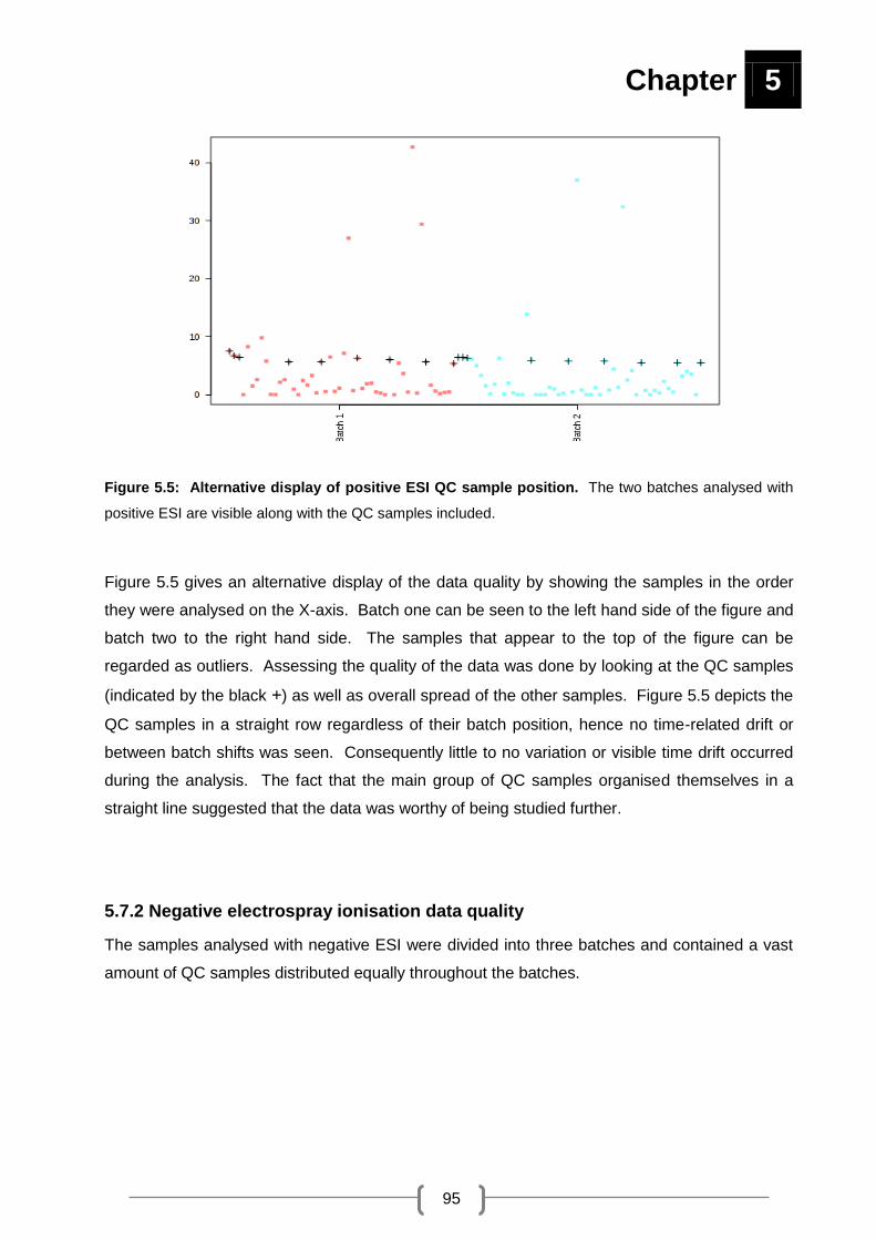
Chapter 5

95

Figure 5.5: Alternative display of positive ESI QC sample position. The two batches analysed with

positive ESI are visible along with the QC samples included.

Figure 5.5 gives an alternative display of the data quality by showing the samples in the order

they were analysed on the X-axis. Batch one can be seen to the left hand side of the figure and

batch two to the right hand side. The samples that appear to the top of the figure can be

regarded as outliers. Assessing the quality of the data was done by looking at the QC samples

(indicated by the black +) as well as overall spread of the other samples. Figure 5.5 depicts the

QC samples in a straight row regardless of their batch position, hence no time-related drift or

between batch shifts was seen. Consequently little to no variation or visible time drift occurred

during the analysis. The fact that the main group of QC samples organised themselves in a

straight line suggested that the data was worthy of being studied further.

5.7.2 Negative electrospray ionisation data quality

The samples analysed with negative ESI were divided into three batches and contained a vast

amount of QC samples distributed equally throughout the batches.

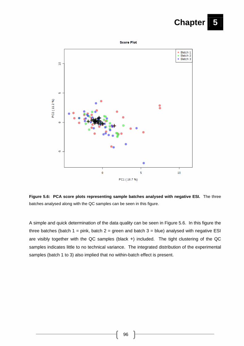
Chapter 5

96

Figure 5.6: PCA score plots representing sample batches analysed with negative ESI. The three

batches analysed along with the QC samples can be seen in this figure.

A simple and quick determination of the data quality can be seen in Figure 5.6. In this figure the

three batches (batch 1 = pink, batch 2 = green and batch 3 = blue) analysed with negative ESI

are visibly together with the QC samples (black +) included. The tight clustering of the QC

samples indicates little to no technical variance. The integrated distribution of the experimental

samples (batch 1 to 3) also implied that no within-batch effect is present.

Chapter 5

97

Figure 5.7: Negative ESI QC sample distribution. QC sample position within the three analysed

batches is displayed in this figure, showing the batch run order on the X-axis.

The three batches analysed with negative ESI are evident in Figure 5.7. From the left to the

right of this figure, batches one to three can be seen. The QC samples are displayed in a semi-

straight line indicating minimal change during analysis. The inclusion of QC samples at the

beginning of the batch allowed conditioning of the column and MS instruments between batches

to take place. This is evident by the few samples that don’t fall in a straight line. Lastly

technical reproducibility was verified, allowing the statistical analyses to proceed since no clear

batch effect was shown.

Since the quality of the data was sufficient for further analysis, no batch- or time-drift corrections

were made to the data. The QC samples were removed and the data from the positive- and

negative ionisation assays pooled to obtain a final data matrix before overview statistics of the

relevant experimental samples were performed. The following sections show the results after

the data of the RCD experimental group was compared to the data of the clinically referred

experimental group, as this was the main objective of this study.

Chapter 5

98

5.7.3 Overview of data before feature selection

The features that remained in the matrix after data cleaning were analysed to visualise any

natural patterns regarding the two relevant experimental groups. An overview of all the features

found in the data matrix before any feature selection step was included can be seen in Figure

5.8.

Figure 5.8: Overview PCA score plot before feature selection process. A combined display of the

RCD patient group and CRC group samples can be seen in the above PCA obtained by a 90%

confidence ellipse.

The smaller cluster of samples (found within the larger group) represents the CRC group (red).

The RCD group (green) is displayed by the samples that are spread out across the plot. It is

expected that the RCD patient group would not cluster together tightly due to the diversity found

RCD CRC

Chapter 5

99

between patients and because RCDs are a heterogeneous group of disorders. Even though

clear separation between the experimental groups isn’t prominent in this case, the tendency of

the groups to group separate is clearly defined. The inclusion of a few RCD samples in the

CRC cluster suggests that some of the RCD patients and CRC have a very similar metabolite

profile which could be expected since these controls were regarded as potential RCD patients

based on the screening tests in the first place.

From a clinical point of view, a ―rule-in‖ approach is preferred for the development of a

biosignature (Pewsner et al., 2004). This means that the developed signature must have a 0%

false negative rate but can have a certain percentage false positive rate. With this approach,

the clinical referred controls with a good probability of having a RCD would be referred for a

biopsy and enzyme confirmation even if it turns out that some do not have respiratory chain

problems in the end.

Another prerequisite of the biosignature is that it must be the smallest set of metabolites that

have the best discrimination power between the groups of interest. More often than not,

diagnosis of other inborn errors of metabolism is based on this principle where the clinician

monitors only a few metabolites mostly related to the defective pathway (Xia et al., 2013).

However, RCDs do not give any pertinent accumulating metabolites and influences the

metabolism in a more global manner as the mitochondrion can be considered as the hub of

metabolism. All the small changes collectively result into the separation of the experimental

groups (Figure 5.8). This hypothesis was also confirmed when supervised statistical methods

used more than a 100 metabolites in discrimination signatures or models (Figure 5.9).

The discrimination power of the evaluated signatures by the supervised multivariate statistical

test is shown in ROC curve format in Figure 5.9. The six graphs (AUC) displayed in Figure 5.9

each represent a sensitivity / specificity value to a particular decision threshold. Graphs

representing 100 (maximum), 50, 25, 15, 10 and 5 features are visible in Figure 5.9. The closer

the ROC curve moves to the upper left corner, the higher the overall accuracy of the test (and

the larger the AUC). Here the results indicate that the best signatures were those that

contained 100 features (variables). The fewer features the test used in the signature, the worse

the modelling became.

Chapter 5

100

Figure 5.9: Multivariate AUC before feature selection. The performance and confidence intervals of

different amount of features are shown in the AUC in this figure.

Figure 5.10: Average predictive accuracies during model cross validation with different number

of features. The predictive accuracy from 5 to 100 features can be viewed in this figure.

Chapter 5

101

This random sub-sampling cross validation displayed in Figure 5.10, tests the performance of

the model created with different number of features (Figure 5.9). Thus Figure 5.10

complements Figure 5.9. From Figure 5.9 it is evident that the more features the signature

contains, the better the model performs. It is clear in Figure 5.10 that the use of 5 features to

distinguish RCD patients and CRC from each other will have on average a 53.9% success rate.

The use of 10, 15, 25 and 50 features have a 59.5%, 61.4%, 64.5% and 72.8% success rate,

respectively. When using 100 features the best average predictive accuracy of 82.9% was

found, the red dot thus indicated the best classifier.

Considering the practical implication of measuring more than a 100 features to best discriminate

patients, a shortlist of about 2 to 10 features would be more practical for clinical testing (Xia et

al., 2013). In order to find the smallest biosignature that can discriminate between the groups in

the best way, feature selection was performed using several univariate and multivariate tests.

5.7.4 Univariate and multivariate feature selection

In Figure 5.11 and Figure 5.12 Venn diagrams were used to illustrate the relationship between

features found by using different statistical methods. The goal was not to use the Venn

diagrams to identify the common features found between the different tests, but merely to give

an illustration of the amount of features found with the various methods. In metabolomics

studies, the amount of features found in the centre of a Venn diagram is commonly considered

to be the most important features in the data. However since, the univariate and multivariate

tests are considered to be complementary to each other and not as tests that are ―correcting

each other‖, this method (of using only the amount of features found in the middle of a Venn

diagram) was not used for feature selection.

Chapter 5

102

Figure 5.11: Univariate and multivariate Venn diagrams of features with significance. Figure A

represents the features detected by using univariate methods. Figure B represents the features found

with the use of multivariate methods.

Figure 5.11.A summarises the features found by using univariate (t-test, effect size and area

under the ROC curve) methods. A total of 27 features were found with the use of a t-test, 1

feature was found when using effect size and 21 features were found with area under the ROC

curve analysis. This adds up to a total of 37 features that can be regarded as important with

univariate methods. In Figure 5.11.B all the features found with the multivariate methods

(random forest, PLS-DA and bivariate AU-ROC curve) are present. With the help of random

forest 50 features were identified, PLS-DA found 79 features and lastly 17 features were

detected by using the bivariate area under the ROC curve analysis. The multivariate methods

ensured a total of 110 features that can be considered as important.

A B

Chapter 5

103

Figure 5.12: Combined Venn diagram of features found. A summary of features found with univariate

and multivariate methods are displayed in this figure.

A combined display of the important features found with univariate and multivariate methods

can be seen in Figure 5.12. Both univariate and multivariate methods assisted in the feature

selection process. Combining the results obtained in Figure 5.11.A and Figure 5.11.B a total of

111 important features were found. This number of 111 features was used to further narrow the

number of features (this will be discussed later) to find a more practical and useful feature list.

A summary of the 111 features found is listed in Appendix A.

5.7.5 Final feature selection

One of the most crucial steps in a metabolomics study is the accurate selection of biomarker

candidates, since it determines the outcome of the current study as well as the course of

validation studies which may follow in the future (Christin et al., 2013). As mentioned, after

feature selection, 111 features were identified to be important and their average rank

determined. The features were sorted according to their average ranking and the graph below

(Figure 5.13) was constructed to identify the number of features that would be most sufficient to

use as a biosignature.

Chapter 5

104

Figure 5.13: Graph display of feature ranking. Using the average ranking of found features the top 12

features presented the best values.

As there is no measure to determine the number of features in the biosignature, the graph

above was used as a guideline. By plotting the feature against the average ranking position, it’s

prominent that the first 12 features (pin pointed by the red oval) on the graph ranked at the top

of the list. The list of 12 features found is listed in Table 5.2 (Section 5.7.6).

Chapter 5

105

5.7.6 Proposed biosignature

The top 12 features selected for the biosignature is listed in Table 5.2. The feature’s annotated name, mass, retention time, effect size d-value, t-

test P-value and PLS-DA VIP value and AUC are included in the table.

Table 5.2: Metabolite markers identified

Annotated name Mass RT Separation

method

Effect size

(d-value)

t-test

(P-value)

PLS-DA

(VIP)

AUC

1 AMP 347.0616 2.30 RP 0.7450 0.0081 2.0351 0.8782

2 C9H19NO 157.1464 30.3 RP 0.5857 0.0102 2.0162 0.8750

3 C23HNO8S4 546.856 12.7 RP 0.6145 0.0194 1.8464 0.8653

4 N-Acetyl asparagine 174.0641 8.7 HILIC 0.9597 0.0031 2.4327 0.9070

5 Unknown 1 1043.4677 11.97 RP 0.6062 0.0243 1.6806 0.8429

6 N-succinyl-L-L2.6 diaminopimelate 290.1126 26.9 RP 0.6152 0.0473 1.4432 0.7307

7 C16H26O4S 314.1547 24.9 RP 0.4790 0.1097 < 1 < 0.7

8 Unknown 2 136.1248 27.9 RP 0.7145 0.0034 2.2290 0.8814

9 C14H22O2 222.1615 24.7 RP 0.7012 0.0066 2.0527 0.8814

10 C14H24O2S 256.1491 27.67 RP 0.4921 0.0588 < 1 < 0.7

11 C20H29NO10 443.1786 21.7 RP 0.7352 0.0143 1.9285 0.8717

12 Oxoglutaric acid 146.0215 2.35 HILIC 0.7882 0.0213 1.7953 0.8589

Chapter 5

106

In the first column the annotated names of the found features are listed where applicable.

These names were assigned to features after a series of identification steps were completed

(Section 5.6). The next column represents the mono-isotopic mass of the selected features.

This mass was assigned to the specific feature during the LC-Q-TOF analysis process. In

column three the retention time at which the feature was found are shown. The fourth column

displays with what separation method the features were found, with RP representing a reverse

phase column in positive ion mode and HILIC a HILIC column using negative ion mode. Next

the d-value obtained after effect size analysis for each feature is shown, followed by t-test P-

value. VIP values obtained by the PLS-DA are displayed next. In the last column the AUC of

the selected features can be found.

Evaluating the annotated names given to the set of features, it was not possible to give a clear

identification to all of the features. As mentioned, the selected ionisation conditions for

untargeted analysis are not optimal for all analysed compounds leading to some fragmentation.

Hence, most of these unidentified features are believed to be fragments of compounds.

Additionally, it appears that most of these fragments might originate from di- and tri-peptides

which are to be expected in patients with muscle-linked phenotypes. Protein degradation is

normally increased in RCD patients, which can also make these good markers. However, it is

not within the scope of this study to interpret the origin or reason for the variance between the

experimental groups. In such a study, all compounds that differed significantly would be

included in pathway analysis for a better understanding of the biological responses.

Furthermore, in order to give a clear biological interpretation of this feature list, validation of the

compound identities are necessary. Possible validation steps will be discussed in Chapter 6.

Chapter 5

107

5.7.7 Evaluating the signature’s discrimination power

To verify if this proposed signature of 12 features can be used to distinguish respiratory chain

deficient patients and clinical referred controls from each other, PCA and multivariate ROC

curves were used.

Figure 5.14: PCA score plot of the proposed signature. Separation of RCD patients and CRC with

the use of the 12 selected features is displayed.

Figure 5.14 shows the PCA score plot of the respiratory chain deficient patients and clinical

referred controls when using only the 12 features found. The smaller circled group to the top of

the figure represents the CRC group (red). The larger circled group to the middle of the figure

represents the RCD patient group (green). With the use of a 90% confidence ellipse, four of the

CRC samples are included within the RCD patient group classification while nine were not. As

discussed previously, complete separation of the groups is not necessarily needed nor possible

RCD CRC

Chapter 5

108

seeing the close enzyme activity scores of CRC to actual positive RCD cases exist. This

implies that these four patients included in the CRC group will also be sent for muscle biopsies

which will be analysed with enzyme analysis to confirm their true diagnosis.

Figure 5.15: ROC curve for the proposed biosignature. By using this curve the proposed signature of

12 features are evaluated with regard to sensitivity and specificity.

The discrimination power of the biosignature is shown in Figure 5.15. The AUC of 0.991 with

95% confidence interval that range between 0.92 and 1 indicates that this signature is both very

specific and sensitive and can be regarded as excellent. It can also be noted that this proposed

signature has 98% sensitivity at 80% specificity, making this a statistically valid method for

biomarker performance. Hence, with the ―rule-in‖ clinical approach, this test will basically

include only 20% false positive cases for biopsy and enzymatic analysis with basically 100% of

the true positive cases (similar to what the PCA score plot indicated).

Chapter 5

109

Figure 5.16: Average predicted class probability of RCDs and clinical referred controls over 100

cross validations. The predicted class probabilities for each sample using the 12 features are shown.

The average predicted class probability (X-axis) of each sample (Y-axis) across 100 cross

validations can be seen in Figure 5.16. On the left side of this figure the CRC sample group ()

can be seen. To the right side the samples classified as RCDs () are visible. The cross

validation algorithm used a balanced sub-sampling approach with the classification boundary at

the centre (0.5). Ranging from 0 to 1 a probability score is calculated, where less than 0.5 will

belong to the CRC and more than 0.5 will belong to the RCD group. This result indicates that

the biosignature was able to classify the samples 100% accurately (on average) in the 100

cross validation sub-samples of the original data (also visualised in the confusion matrix below).

In order to further evaluate the performance of the proposed signature a two class-confusion

matrix (Table 5.3) was compiled. The contingency table (confusion matrix) is ultimately used to

summarise the predictive performance of the biosignature on the specific test data used.

CRC RCD

Chapter 5

110

Table 5.3: Two-class confusion matrix

PREDICTED

0 (CRC) 1 (RCD)

0 (CRC) 13 (TN) 0 (FN)

1 (RCD) 0 (FP) 24 (TP)

The number of instances for each of the four possible classification outcomes can be seen in

Table 5.3. These classifications are known as: true positive (TP) – where the number of

diseased patients is correctly detected as diseased; false positive (FP) – in this case the

number of healthy cases is incorrectly described as diseased; false negative (FN) – the

number of diseased patients is wrongly identified as healthy and lastly true negative (TN) –

here the amount of healthy cases is rightfully identified as healthy (Xia et al., 2013). Each

prediction of a confusion matrix represents one point on a ROC curve. The 13 clinical referred

control samples (represented by 0) were all classified as true negative cases, so these patients

were positively predicted. The 24 RCD patient samples (represented by 1) were found to be

true positive cases. To evaluate the accuracy of this confusion matrix the following calculation

can be performed: Accuracy = (TP + TN) / (TP + TN + FP + FN). By using the information

above the accuracy of this matrix is 100% (Fawcett, 2006). Consequently when evaluating the

performance of this biosignature on this specific data matrix the accuracy of correctly classified

patterns is 100% in the cross validation process.

Next, permutation testing was used to validate the proposed signature performance as another

form of cross-validation. This technique is based on the hypothesis that this proposed set of

biomarkers could have been found again if every patient or control sample had been randomly

assigned to a different group (Xia et al., 2013). To prove or disaprove this hypothesis, 1 000

models were permuted, by randomly assigning each sample to an experimental group and then

using the proposed signature for the classification of the dummy groups. As a result a

reference distribution (of the null hypothesis) is given to be compared to the correctly assigned

model, which leads to a P-value. With a P-value < 0.05 a randomly permuted outcome variable

has less than 5% chance to produce a model of similar performance to the correctly assigned

model (Xia et al., 2013). The outcome of the permutation test is given in Figure 5.17.

Chapter 5

111

Figure 5.17: Permutation test of the proposed biosignature. An AUC achieved by means of a

permutation test is seen here with a P < 0.01.

Figure 5.17 displays 1 000 permuted tests (represented by the dashed lines found above)

performed. The proposed signature resulted in a permutation test value of P < 0.01, thus by

using random guessing there is 1% chance to produce the same model indicating the specificity

of the biosignature. Lastly it can be verified that in the use of 1 000 permutation tests none of

the results performed better than the original design, thus a P-value of P < 0.01 was reported.

In all of the results obtained above SVM was used as the underlying multivariate algorithm. To

ensure that this test did not have any bias toward the specific data, PLS-DA was also tested in

the multivariate ROC modelling. The use of PLS-DA over SVM produced the exact same

results.

Chapter 5

112

5.8 IMPLEMENTING THE SIGNATURE ON A PRACTICAL EXAMPLE

An alternative experimental group included in this study was patients with neuromuscular

disorders. These disorders affects the peripheral nervous system potentially influencing

muscles, nerve-muscle junctions, peripheral nerves and motor-nerve cells in the spinal cord.

On a clincal level patients with a suspected RCD and patients suffering from other

neuromuscular disorders can be differentiated in many circumstances, but if a physician is

unable to distingish these patients the proposed signature may be helpful. In order to verify if

the signature of 12 features would be useful to differentiate a RCD patient from a patient with a

neuromuscular disorder, the proposed signature was implemented on a group of patients

including those with genetically confirmed Duchenes muscular dystrophy and spinal muscular

atrophy as well as patients with histologically confirmed dermatomyositis or polymiositis. The

results obtained by this alternative approach are shown in Figure 5.18 and 5.19 (obtained in the

same manor as the RCD vs CRC).

Figure 5.18: 3D PCA score plot of the three experimental groups analysed. The clinical referred

control group, the neuromuscular disorder group and the respiratory chain deficient patient group can be

seen on the PCs above.

CRC NMD RCD

Chapter 5

113

The three experimental groups analysed as part of this untargeted LC-MS investigation are

shown in the 3D PCA score plot displayed in Figure 5.18. The CRC group (red ), NMD group

(green ) and RCD group (blue ) are demonstrated in the figure above. By using the 12

features found with a variety of statistical methods it is possible to successfully separate RCDs

and the CRC in the figure found above, since the CRC group appears to the top of the figure

and the RCD group is displayed to the middle/bottom. This is an expected result since

biosignatures designed for a specific population are largely applicable to that target population.

By using a PCA it is not possible to separate RCD patients and patients with NMD (Figure

5.18). In the PCA shown in Figure 5.18 it is observed that the neuromuscular disorder samples

are spread out amongst the two remaining experimental groups. The samples represented by

the neuromuscular disorder patients do not cluster together, suggesting that a large amount of

variation is found within this group. This variation may be present due to the fact that the

neuromuscular disorder group contained patients with three different neuromsucular disorders

(dermatomyositis, Duchene muscular dystrophy and spinal muscular atrophy) or that they may

have secondary RCDs.

An alternative technique was also used to determine if the signature had the potential to identify

RCD patients from patients with neuromuscular disorders. Model discrimination was

determined by examining the AUC by using 95% confidence intervals (visible in Figure 5.19).

Chapter 5

114

Figure 5.19: AUC of patients with neuromuscular disorders. Patients with neuromuscular disorders

were distinguished from patients with RCDs on this basis of the proposed biosignature.

The AUC used in Figure 5.19 show the probability of the proposed 12 feature biosignature to be

used as a diagnostic model when discriminating between RCD patients and patients with NMD.

It is now known that the larger the AUC the better the overall performance of a test. Generally

as the AUC becomes smaller the performance of a specific test tends to decrease. The use of

the 12 selected features resulted in an AUC value of 0.782. This model can be regarded as a

fair signature to use to differentiate RCD cases from patients with neuromuscular disorders.

Certainly it is not expected that the biosignature designed to discriminate between RCD patients

and CRC result in an AUC of > 0.9 when used on neuromuscular disorder patients. This AUC

shows 90% sensitivity for distinguishing neuromuscular disorder cases from RCD patients when

40% specificity is achieved. By using this model, 60% false positives (patients that do not have

a RCD) will be included in the selection to receive a muscle biopsy and 90% of the cases will be

true positive (patients with a RCD).

Chapter 5

115

Ultimately the main idea of this diagnostic screening test is to increase (or decrease) the

suspicion of a RCD from the patients that present with associated symptoms, in order to make

management decisions regarding the affected patients and this can be achieved with the new

proposed biosignature.

116

CHAPTER 6:

Conclusion

Chapter 6

117

6.1 INTRODUCTION

Mitochondrial disorders like RCDs (which can be regarded as a sub-group of mitochondrial

disorders) can present at any age with single or combined symptoms in most organ systems.

As a result of the heterogeneity of RCDs, diagnosis of these disorders is complicated and

requires a multidisciplinary approach consisting of clinical, histochemical, biochemical and

molecular assessment. Currently enzyme analysis on a muscle sample is one of the best

methods for confirming a RCD. This highly invasive diagnostic procedure comes with a number

of limitations, which makes the search for a less invasive method a necessity. Taking into

consideration that urine samples provide minimal invasiveness as well as other practical

advantages (like ease of sample storage and transportation), the aim of this study was to use

an untargeted LC-MS metabolomics approach to investigate respiratory chain deficiencies in

children from South Africa. In order to achieve this aim the following objectives were

undertaken. Firstly: positive- and negative electrospray ionisation techniques using a

quadrupole time-of-flight mass spectrometer had to be standardised. Secondly: urine samples

of children suffering from respiratory chain deficiencies alongside urine from different control

groups had to be analysed. Thirdly: a list of features distinguishing RCD patients and clinical

referred controls from each other had to be compiled.

6.2 CONCLUSIONS

In conclusion a summary of the main findings of Chapters 3, 4 and 5 along with their connection

to the objectives achieved in this study will be provided together with future recommendations.

6.2.1 Standardisation procedures

Metabolomics research workflow generally involves a number of steps ranging from sample

extraction to biomarker discovery. In order to assure that the workflow can be followed

efficiently a number of different factors had to be investigated. The first objective of this study

was to standardise both positive- and negative electrospray ionisation techniques using a

quadrupole time-of-flight mass spectrometer. In order to achieve this objective, four goals

concerning the methods used had to be reached.

Chapter 6

118

Firstly, a decision regarding MFE or MFE in combination with FbI as a data extraction method

had to be made. With the help of a few experiments described in Chapter 3 it was decided that

MFE in combination with FbI was the best data extraction method to use. A study done by

Kitagawa et al., (2009) supports the findings of this study. They found that initial feature

extraction by means of the MFE algorithm needed to be accompanied by a re-extraction step

using a different targeted algorithm like FbI. This approach ultimately improved the mass

spectrometric feature extraction conducted on large data sets (Kitagawa et al., 2009).

Secondly, minimum sample preparation was compared with organic acid extraction

(fractionation) in order to find a suitable sample extraction method. Theodoridis et al., (2012)

stated that ideally minimal sample preparation should be used when doing LC-MS experiments

to ensure that the composition of the sample of interest is not altered in any way. When using

urine they deemed centrifugation and dilution as sufficient (Theodoridis et al., 2012). This

statement correlated with what was found in Chapter 3, showing that minimum sample

preparation outperformed fractionation as a sample extraction method.

Thirdly, an appropriate modifier for negative ESI had to be identified. The modifiers under

investigation in Chapter 4 included acetic acid (17 mM and 5 mM) and 5 mM ammonium

acetate (pH 4.5 and 7.0). Water and acetonitrile enriched with 5 mM acetic acid was selected

as LC-Q-TOF reagents when doing negative ESI. An optimal additive for metabolomics studies

in negative ion mode was reported by Zhang et al., (2012) as 1 mM acetic acid. Wu et al.,

(2004) noted that the weaker acids (like acetic acid) in concentrations from 10 µM to 10 mM

enhanced negative ESI responses (with 1 mM presenting maximum ESI responses).

Furthermore Yanes et al., (2011) experimented between 1 mM ammonium fluoride and 5 mM

ammonium acetate, selecting 1 mM ammonium fluoride as best modifier since it displayed the

highest sensitivity and due to the fact that 5 mM (or higher) introduced background into the

mass spectra. Due to conflicting findings in the literature and results obtained by this study, 5

mM acetic acid was shown to be the mobile phase modifier to use in this case.

Fourthly, the use of a HILIC column in negative ESI had to be evaluated. An experiment

conducted by Saric et al., (2012) showed that the use of both reverse phase- and HILIC

columns, were complementary in an attempt to gain maximum metabolite coverage. Cubbon et

al., (2007) suggested that HILIC columns should be used as a complementary separation

method to reverse phase columns, as polar compounds are commonly missed with only reverse

phase columns. Negative ionisation also added value to their findings and should thus also be

used to ensure the most comprehensive data. It is clear that the use of both a HILIC- and a

reverse phase column is highly recommended, since it would allow the retention and separation

Chapter 6

119

of as many features as possible. The use of a reverse phase- and a HILIC column was

successfully applied in Chapter 4 of this study. The use of both positive ESI and negative ESI

can also be regarded as a popular choice for metabolomics studies. The nature of some

analytes prefers positive ESI for ionisation, while other compounds ionise better by using

negative ESI (Theodoridis et al., 2012). Both positive and negative ESI were implemented in

this study. Keeping in mind that no single method can ensure complete metabolome coverage,

Saric et al., (2012) exhibited that by using a reverse phase- and a HILIC column in both

ionisation modes a large number of metabolites can be detected. The use of both columns in

both ESI modes did not form part of the experimentation process in this study and can be seen

as an area in need of improvement.

6.2.2 Experimental group selection and analysis

In Chapter 5 of this metabolomics study three experimental groups were selected (respiratory

chain deficient patient group, clinical referred control group and a neuromsucular disorder

group), but the main focus was on the RCD patient group and the CRC group. If healthy

controls (with no suspected RCD) were chosen in this study instead of CRC, a much higher

specificity could be expected from the test results. It is clear that controls selected for an

experiment should not have the target disease (RCD), but if all conditions that the test might

confuse with the disease are also excluded by the control group (like when using healthy

controls) the test will be too optimistic (Goroll and Mulley, 2009). Due to the fact that urine

samples of the patient and the clinical referred control group was selected from the target

population presenting with RCD symptoms, it is certain that no bias for a specific result was

obtained. It is possible to say that the correct patient and control groups for the aim of this

study were selected making the results obtained even more plausible. Furthermore this

selection made it possible to conduct the second objective (of this study) of analysing urine

samples of children with RCD and different control groups successfully.

Still focusing on the second objective, urine had to be analysed in an untargeted fashion with

the use of a LC-Q-TOF. Untargeted methods aim to find features of all detectable compounds

at the time of measurement making this approach appropriate for finding changes in the

metabolome (Schuhmacher et al., 2013). The use of time-of-flight analysers make it probable

to obtain high sensitivity spectra without trouble and along with the high mass accuracy

determining molecular formulas for molecules are possible (Pitt, 2009). Thus the use of a LC-

Q-TOF instrument can be regarded as the best analytical apparatus to use in an untargeted

metabolomics experiment.

Chapter 6

120

6.2.3 Feature selection

The third objective of this study was to compile a list of features that can distinguish RCD

patients for clinical referred controls. Without a good feature selection approach conducted by a

number of statistical methods, it would not have been possible to achieve this objective. The

methods used for feature selection (t-test, effect size, area under the ROC curve, random

forest, PLS-DA and bivariate AU-ROC curve) can be seen in Chapter 5. In a study conducted

by Christin et al., (2013), PLS-DA displayed good precision as a feature selection method but

was said to miss features that could be informative. This was prevented in the present study by

including univariate feature selection methods which made it possible to identify biomarker

candidates with high confidence. Furthermore Christin et al., (2013), reported that SVM

performed poorly when used to select relevant features. In light of their observation SVM was

not used as a feature selection method but rather as a method to test and display the found

features. Random forest received much praise as a suitable classification and biomarker

selection tool for metabolomics data analysis by Chen et al., (2013) and formed part of the

network of methods used in this study to select the best possible features. Considering that a

group of 12 features (Table 5.3) were found by combining multiple methods, it can be noted that

the feature selection process was sufficient.

6.2.4 Biomarker discovery

As part of the third objective a list of features had to be compiled, distinguishing RCD patients

and clinical referred controls from each other. This objective was successfully achieved in

Chapter 5, but identification of the 12 features (Section 5.7.5) found to be biomarkers was not

completed as it did not fall in the scope of this study. The question that needs to be asked at

this stage is whether it is really possible to detect 12 features when investigation RCDs?

Suomalainen (2011) stated that it would be improbable to find a single biomarker that could be

relevant to a highly diverse disease group like RCDs. The search for a group of biomarkers

(biosignature) can be seen as the way forward for biomarker discovery concerning RCDs.

When investigating inborn errors of metabolism it is very likely to find a single metabolite marker

because of the huge difference in the concentration of the specific biomarker found between

normal and diseased (Xia et al., 2013). A respiratory chain deficiency can to some extent be

classified as an inborn error of metabolism. In no way would one specific compound show a

concentration built-up in the case of RCDs, but electron (found in the ETC) built-up is likely to

be found. Two electron carriers (NADH and FADH2) are responsible for transporting electrons

Chapter 6

121

into the ETC. Thus when electrons start to build-up the concentration of these electron carriers

tend to increase. However this does not have one single implication, resulting in the increase of

a specific metabolite. Since NADH and FADH2 are involved in a variety of metabolic pathways,

they seem to cope with the electron built up, to some extent. It might be that smaller

concentration changes spread amongst a number of metabolic pathways are taking place,

making it impossible to develop a single biomarker test. Therefore it is more likely that a

combination of metabolites (instead of a single metabolite) can be used to distinguish RCDs

from controls.

The existence of a possible biosignature for RCDs can be confirmed by the putative

biosignature proposed by Smuts et al., (2013). In their study a semi-targeted metabolomics

approach was followed to investigate RCDs resulting in a biosignature of six amino acids, six

organic acids and creatine.

Seeing that the respiratory chain is found within a network of pathways and due to the fact that

a biosignature of 13 metabolites have previously been found, it would be possible to find 12

features associated with RCDs. The ―new‖ found biosignature of 12 features reported in this

study would surely have the potential to develop a cost-effective biomarker test, which would in

the long run be of value to the process of selecting suspected RCD patients that need to

undergo a muscle biopsy to confirm their diagnosis.

6.2.5 Biosignature evaluation

To determine if the proposed biosignature had diagnostic value the AUC was determined. An

AUC of 0.991 with 95% confidence interval was found when using the proposed biosignature to

distinguish between RCD patients and clinical referred controls. This model resulted in an

accuracy of 100% when considering the amount of true positives, false positives, true negatives

and false negatives found in the experimental group. Suomalainen et al., (2011) used ROC

curves to demonstrate the importance of FGF-21 as a potential biomarker for RCDs. The AUC

for FGF-21 was 0.95, stating that there is a 95% chance that FGF-21 serum concentrations will

correctly differentiate between patients with a muscle manifesting mitochondrial disease and

patients with non-mitochondrial disease. Furthermore AUC was used in this study to determine

if the proposed biosignature had the potential to distinguish between RCD patients and patients

with neuromuscular disorders. The AUC for NMD based on the 12 features found was 0.782,

making it 78% accurate to differentiate between the two involved groups. Considering the

aforementioned, ROC curve analysis can be regarded as the correct method to follow to obtain

Chapter 6

122

insights of how good the model will perform on a diagnostic level if it is implemented on the

patient group of interest.

6.2.6 Final conclusion

This study hence, shows that it is possible to use an untargeted LC-MS metabolomics approach

to investigate respiratory chain deficiencies in children from South Africa.

6.3 FUTURE RECOMMENDATIONS

In hindsight of this dissertation, the following recommendations in the interest of future studies

concerning this work investigated can be made.

When doing an untargeted metabolomics study the aim is to get maximum coverage of the

metabolome. A wider coverage can be obtained when one uses both ESI methods for reverse

phase and HILIC columns. Even though overlapping in the results are expected it is likely that

these four data matrices would complement each other and add value to the results.

In order to achieve the best possible results, the control and patient selection process can be

regarded as an area where improvement is possible. In an ideal world it would be the aim to

have control and experimental groups that are as homogenous as possible. This would enable

comparison with regard to age, ethnicity, diet, gender, lifestyle habits and other possibilities that

may influence the results. In most cases it is not possible to select a reasonable experimental

group and keep the group homogenous as well. Nevertheless the inclusion of controls that

mimic patients to the closest extent may show new insight regarding the metabolism of RCDs.

In this current study a list of 12 features were identified as important to distinguish patients and

controls from one another. These features were classified on the basis of their accurate

masses and/or retention times and/or annotated names. One problem that needs to be

addressed is identification of these features by using additional information for example

fragmentation spectra. This can be achieved with the use of an Ion Trap or Synapt of All ions

MS/MS instrument, which collects fragmentation data that can be used to determine the true

identification of a feature.

Chapter 6

123

Next validation would also be required to reach a functional model. Validation can be achieved

by a number of different approaches. Firstly a laboratory repeatability study can be performed.

Here the same samples, on the same instrument, by the same observer in the same laboratory

are used to measure the observed features. Secondly a laboratory replication study can be

performed. In this case independent samples are analysed on the same instrument by the

same observer. A third validation study is an inter-laboratory repeatability study. This study

uses the same samples (as in the original study), but a different instrument, in a different

laboratory by a different observer. The fourth level of validation would be an inter-laboratory

replication study. Now a new set of test subjects will be analysed in a different laboratory on a

different instrument by a different observer (Xia et al., 2013). Ultimately validation needs to

evaluate the markers found to be a biosignature.

The practical implementation of this biosignature also needs to be determined. One way of

using this biosignature to differentiate between two patients in a diagnostic situation, would be

with the use of a linear algebra equation (like logistic regression) were a numeric value would

indicate the state of the patient.

124

CHAPTER 7:

References

Chapter 7

125

ABDI, H. & WILLIAMS, L. J. 2010. Principal component analysis. Wiley Interdisciplinary Reviews: Computational Statistics, 2, 433-459.

AGILENT-TECHNOLOGIES. 2012. TOF and Q-TOF preparation - calibration and tuning [Online]. USA: Agilent technoliges Inc. G3335-90142. Available: http://www.chem.agilent.com/Library/usermanuals/Public/G3335-90142_TOF_Q-TOF_Concepts.pdf.

ÁLVAREZ-SÁNCHEZ, B., PRIEGO-CAPOTE, F. & LUQUE DE CASTRO, M. D. 2010. Metabolomics analysis I. Selection of biological samples and practical aspects preceding sample preparation. TrAC Trends in Analytical Chemistry, 29, 111-119.

BANDYOPADHYAY, S. & DUTTA, A. 2010. Mitochondrial Medicine. JAPI, 58, 237.

BOLISETTY, S. & JAIMES, E. A. 2013. Mitochondria and Reactive Oxygen Species: Physiology and Pathophysiology. International journal of molecular sciences, 14, 6306-6344.

BOUATRA, S., AZIAT, F., MANDAL, R., GUO, A. C., WILSON, M. R., KNOX, C., BJORNDAHL, T. C., KRISHNAMURTHY, R., SALEEM, F. & LIU, P. 2013. The Human Urine Metabolome. PloS one, 8, e73076.

BUSZEWSKI, B. & NOGA, S. 2012. Hydrophilic interaction liquid chromatography (HILIC)—a powerful separation technique. Analytical and bioanalytical chemistry, 402, 231-247.

CHEN, J., WANG, W., LV, S., YIN, P., ZHAO, X., LU, X., ZHANG, F. & XU, G. 2009. Metabonomics study of liver cancer based on ultra performance liquid chromatography coupled to mass spectrometry with HILIC and RPLC separations. Analytica Chimica Acta, 650, 3-9.

CHEN, T., CAO, Y., ZHANG, Y., LIU, J., BAO, Y., WANG, C., JIA, W. & ZHAO, A. 2013. Random Forest in Clinical Metabolomics for Phenotypic Discrimination and Biomarker Selection. Evidence-Based Complementary and Alternative Medicine, 2013.

CHINNERY, P. & SCHON, E. 2003. Mitochondria. Journal of Neurology, Neurosurgery & Psychiatry, 74, 1188-1199.

CHRISTIN, C., HOEFSLOOT, H. C., SMILDE, A. K., HOEKMAN, B., SUITS, F., BISCHOFF, R. & HORVATOVICH, P. 2013. A critical assessment of feature selection methods for biomarker discovery in clinical proteomics. Molecular & Cellular Proteomics, 12, 263-276.

CUBBON, S., BRADBURY, T., WILSON, J. & THOMAS-OATES, J. 2007. Hydrophilic interaction chromatography for mass spectrometric metabonomic studies of urine. Analytical chemistry, 79, 8911-8918.

DEJAEGHER, B. & VANDER HEYDEN, Y. 2010. HILIC methods in pharmaceutical analysis. Journal of separation science, 33, 698-715.

DETTMER, K., ARONOV, P. A. & HAMMOCK, B. D. 2007. Mass spectrometry-based metabolomics. Mass Spectrometry Reviews, 26, 51-78.

http://www.chem.agilent.com/Library/usermanuals/Public/G3335-90142_TOF_Q-TOF_Concepts.pdf

http://www.chem.agilent.com/Library/usermanuals/Public/G3335-90142_TOF_Q-TOF_Concepts.pdf

Chapter 7

126

DIAZ, F., KOTARSKY, H., FELLMAN, V. & MORAES, C. T. Mitochondrial disorders caused by mutations in respiratory chain assembly factors. Seminars in Fetal and Neonatal Medicine, 2011. Elsevier, 197-204.

DIMAURO, S. & SCHON, E. A. 2003. Mitochondrial Respiratory-Chain Diseases. New England Journal of Medicine, 348, 2656-2668.

DO YUP LEE, B. P. B. & NORTHEN, T. R. 2010. Mass spectrometry–based metabolomics, analysis of metabolite-protein interactions, and imaging. Biotechniques, 49, 557.

DOERFLER, H., LYON, D., NÄGELE, T., SUN, X., FRAGNER, L., HADACEK, F., EGELHOFER, V. & WECKWERTH, W. 2012. Granger causality in integrated GC–MS and LC–MS metabolomics data reveals the interface of primary and secondary metabolism. Metabolomics, 1-11.

DUNN, W., ERBAN, A., WEBER, R. M., CREEK, D., BROWN, M., BREITLING, R., HANKEMEIER, T., GOODACRE, R., NEUMANN, S., KOPKA, J. & VIANT, M. 2013a. Mass appeal: metabolite identification in mass spectrometry-focused untargeted metabolomics. Metabolomics, 9, 44-66.

DUNN, W. B., BAILEY, N. J. C. & JOHNSON, H. E. 2005. Measuring the metabolome: current analytical technologies. Analyst, 130, 606-625.

DUNN, W. B., BROADHURST, D., BEGLEY, P., ZELENA, E., FRANCIS-MCINTYRE, S., ANDERSON, N., BROWN, M., KNOWLES, J. D., HALSALL, A., HASELDEN, J. N., NICHOLLS, A. W., WILSON, I. D., KELL, D. B. & GOODACRE, R. 2011a. Procedures for large-scale metabolic profiling of serum and plasma using gas chromatography and liquid chromatography coupled to mass spectrometry. Nat. Protocols, 6, 1060-1083.

DUNN, W. B., BROADHURST, D. I., ATHERTON, H. J., GOODACRE, R. & GRIFFIN, J. L. 2011b. Systems level studies of mammalian metabolomes: the roles of mass spectrometry and nuclear magnetic resonance spectroscopy. Chemical Society Reviews, 40, 387-426.

DUNN, W. B., ERBAN, A., WEBER, R. J., CREEK, D. J., BROWN, M., BREITLING, R., HANKEMEIER, T., GOODACRE, R., NEUMANN, S. & KOPKA, J. 2013b. Mass appeal: metabolite identification in mass spectrometry-focused untargeted metabolomics. Metabolomics, 9, 44-66.

DUNN, W. B., WILSON, I. D., NICHOLLS, A. W. & BROADHURST, D. 2012. The importance of experimental design and QC samples in large-scale and MS-driven untargeted metabolomic studies of humans. Bioanalysis, 4, 2249-2264.

ELLIS, S. & STEYN, H. 2003. Practical significance (effect sizes) versus or in combination with statistical significance (p-values). Management dynamics, 12, 51-53.

FAWCETT, T. 2006. An introduction to ROC analysis. Pattern recognition letters, 27, 861-874.

FIEHN, O. 2002. Metabolomics–the link between genotypes and phenotypes. Plant molecular biology, 48, 155-171.

Chapter 7

127

FREY, T. G. & MANNELLA, C. A. 2000. The internal structure of mitochondria. Trends in Biochemical Sciences, 25, 319-324.

GAMA, M. R., DA COSTA SILVA, R. G., COLLINS, C. H. & BOTTOLI, C. B. 2012. Hydrophilic interaction chromatography. TrAC Trends in Analytical Chemistry, 37, 48-60.

GOROLL, A. H. & MULLEY, A. G. 2009. Selection and interpretation of diagnostic tests. Primary Care medicine - Office evaluation and management of the adult patient. 6 ed.: Lippincott Williams & Wilkins.

HAAS, R. H., PARIKH, S., FALK, M. J., SANETO, R. P., WOLF, N. I., DARIN, N. & COHEN, B. H. 2007. Mitochondrial disease: a practical approach for primary care physicians. Pediatrics, 120, 1326-1333.

HAAS, R. H., PARIKH, S., FALK, M. J., SANETO, R. P., WOLF, N. I., DARIN, N., WONG, L.-J., COHEN, B. H. & NAVIAUX, R. K. 2008. The in-depth evaluation of suspected mitochondrial disease. Molecular genetics and metabolism, 94, 16-37.

HARPER, P. S. 2004. Genetic counselling in mendelian disorders. Practical genetic counselling. Hodder Arnold London.

HOLČAPEK, M., JIRÁSKO, R. & LÍSA, M. 2010. Basic rules for the interpretation of atmospheric pressure ionization mass spectra of small molecules. Journal of Chromatography A, 1217, 3908-3921.

HRYDZIUSZKO, O. & VIANT, M. R. 2012. Missing values in mass spectrometry based metabolomics: an undervalued step in the data processing pipeline. Metabolomics, 8, 161-174.

ISSAQ, H. J., VAN, Q. N., WAYBRIGHT, T. J., MUSCHIK, G. M. & VEENSTRA, T. D. 2009. Analytical and statistical approaches to metabolomics research. Journal of Separation Science, 32, 2183-2199.

JANSSEN, A., SMEITINK, J. & VAN DEN HEUVEL, L. 2003. Some practical aspects of providing a diagnostic service for respiratory chain defects. Annals of clinical biochemistry, 40, 3-8.

KITAGAWA, N., M, S., SANA, F. T., DARLAND, D. P. E. & LI, X. 2009. Improving Untargeted Differential Analysis of Mass Spectrometric Data by Recursive Feature Extraction. Agilent Technologies, Inc., Santa Clara, CA, WPB 061.

KOENE, S. & SMEITINK, J. 2011. Metabolic manipulators: a well founded strategy to combat mitochondrial dysfunction. Journal of inherited metabolic disease, 34, 315-325.

KOENIG, M. K. 2008. Presentation and diagnosis of mitochondrial disorders in children. Pediatric neurology, 38, 305-313.

LEEK, J. T., SCHARPF, R. B., BRAVO, H. C., SIMCHA, D., LANGMEAD, B., JOHNSON, W. E., GEMAN, D., BAGGERLY, K. & IRIZARRY, R. A. 2010. Tackling the widespread and critical impact of batch effects in high-throughput data. Nature Reviews Genetics, 11, 733-739.

Chapter 7

128

LIEBER, D. S., CALVO, S. E., SHANAHAN, K., SLATE, N. G., LIU, S., HERSHMAN, S. G., GOLD, N. B., CHAPMAN, B. A., THORBURN, D. R. & BERRY, G. T. 2013. Targeted exome sequencing of suspected mitochondrial disorders. Neurology, 80, 1762-1770.

LILAND, K. H. 2011. Multivariate methods in metabolomics–from pre-processing to dimension reduction and statistical analysis. TrAC Trends in Analytical Chemistry, 30, 827-841.

LINDEQUE, J. Z., HIDALGO, J., LOUW, R. & VAN DER WESTHUIZEN, F. H. 2013. Systemic and organ specific metabolic variation in metallothionein knockout mice challenged with swimming exercise. Metabolomics, 1-15.

LUDWIG, R., EDGE, T. & PERIER, L. 2011. Investigation into the stability of HILIC based Cetirizine assay [Online]. Thermo Fisher Scientific. Available: http://apps.thermoscientific.com/media/SID/Europe%20Region/PDF/Cetirizine.pdf.

LUFT, R., IKKOS, D., PALMIERI, G., ERNSTER, L. & AFZELIUS, B. 1962. A case of severe hypermetabolism of nonthyroid origin with a defect in the maintenance of mitochondrial respiratory control: a correlated clinical, biochemical, and morphological study. Journal of clinical investigation, 41, 1776.

LUO, J., SCHUMACHER, M., SCHERER, A., SANOUDOU, D., MEGHERBI, D., DAVISON, T., SHI, T., TONG, W., SHI, L. & HONG, H. 2010. A comparison of batch effect removal methods for enhancement of prediction performance using MAQC-II microarray gene expression data. The pharmacogenomics journal, 10, 278-291.

MANNELLA, C. A., LEDERER, W. J. & JAFRI, M. S. 2013. The connection between inner membrane topology and mitochondrial function. Journal of Molecular and Cellular Cardiology, 62, 51-57.

MIHALEVA, V. V., VORST, O., MALIEPAARD, C., VERHOEVEN, H. A., DE VOS, R. C., HALL, R. D. & VAN HAM, R. C. 2008. Accurate mass error correction in liquid chromatography time-of-flight mass spectrometry based metabolomics. Metabolomics, 4, 171-182.

MUNNICH, A., RÖTIG, A., CORMIER-DAIRE, V. & RUSTIN, P. 2011. Clinical Presentation of Respiratory Chain Deficiency. The online metabolic and molecular base of inherited disease, 10.

NEUSTADT, J. & PIECZENIK, S. R. 2008. Medication-induced mitochondrial damage and disease. Molecular Nutrition & Food Research, 52, 780-788.

NEWMAN, M., GORDON, S. & M.S., R. 2004. Urinary Organic Acid Analysis: A Powerful Clinical Tool, Potentially Muddled by Poor Testing Methods. . US BioTek Laboratories, Inc. www.usbiotek.com.

NIELSEN, N. J., TOMASI, G., FRANDSEN, R. J., KRISTENSEN, M. B., NIELSEN, J., GIESE, H. & CHRISTENSEN, J. H. 2010. A pre-processing strategy for liquid chromatography time-of-flight mass spectrometry metabolic fingerprinting data. Metabolomics, 6, 341-352.

NUNNARI, J. & SUOMALAINEN, A. 2012. Mitochondria: In Sickness and in Health. Cell, 148, 1145-1159.

http://apps.thermoscientific.com/media/SID/Europe%20Region/PDF/Cetirizine.pdf

http://www.usbiotek.com/

Chapter 7

129

O’ROURKE, B., CORTASSA, S. & AON, M. A. 2005. Mitochondrial Ion Channels: Gatekeepers of Life and Death. Physiology, 20, 303-315.

PARSONS, H. M., LUDWIG, C., GÜNTHER, U. L. & VIANT, M. R. 2007. Improved classification accuracy in 1-and 2-dimensional NMR metabolomics data using the variance stabilising generalised logarithm transformation. BMC bioinformatics, 8, 234.

PATTI, G. J., YANES, O. & SIUZDAK, G. 2012. Innovation: metabolomics: the apogee of the omics trilogy. Nature Reviews Molecular Cell Biology, 13, 263-269.

PEWSNER, D., BATTAGLIA, M., MINDER, C., MARX, A., BUCHER, H. C. & EGGER, M. 2004. Ruling a diagnosis in or out with ―SpPIn‖ and ―SnNOut‖: a note of caution. BMJ, 329, 209-213.

PIECZENIK, S. R. & NEUSTADT, J. 2007. Mitochondrial dysfunction and molecular pathways of disease. Experimental and Molecular Pathology, 83, 84-92.

PITT, J. J. 2009. Principles and applications of liquid chromatography-mass spectrometry in clinical biochemistry. The Clinical Biochemist Reviews, 30, 19.

REINECKE, C. J., KOEKEMOER, G., VAN DER WESTHUIZEN, F. H., LOUW, R., LINDEQUE, J. Z., MIENIE, L. J. & SMUTS, I. 2012. Metabolomics of urinary organic acids in respiratory chain deficiencies in children. Metabolomics, 8, 264-283.

RODENBURG, R. T. 2011. Biochemical diagnosis of mitochondrial disorders. Journal of Inherited Metabolic Disease, 34, 283-292.

SACCENTI, E., HOEFSLOOT, H. C., SMILDE, A. K., WESTERHUIS, J. A. & HENDRIKS, M. M. 2013. Reflections on univariate and multivariate analysis of metabolomics data. Metabolomics, 1-14.

SAEED, S. & SINGER, M. 2013. Mitochondria — key roles in sepsis. Réanimation, 22, 352-358.

SANA, T. & FISCHER, S. 2007. Maximizing metabolite extraction for comprehensive metabolomics studies of erythrocytes. Agilent Technologies research applications, 5989.

SARIC, J., WANT, E. J., DUTHALER, U., LEWIS, M., KEISER, J., SHOCKCOR, J. P., ROSS, G. A., NICHOLSON, J. K., HOLMES, E. & TAVARES, M. F. 2012. Systematic Evaluation of Extraction Methods for Multiplatform-Based Metabotyping: Application to the Fasciola hepatica Metabolome. Analytical chemistry, 84, 6963-6972.

SCALBERT, A., BRENNAN, L., FIEHN, O., HANKEMEIER, T., KRISTAL, B. S., VAN OMMEN, B., PUJOS-GUILLOT, E., VERHEIJ, E., WISHART, D. & WOPEREIS, S. 2009. Mass-spectrometry-based metabolomics: limitations and recommendations for future progress with particular focus on nutrition research. Metabolomics, 5, 435-458.

SCHAEFER, A. M., TAYLOR, R. W., TURNBULL, D. M. & CHINNERY, P. F. 2004. The epidemiology of mitochondrial disorders—past, present and future. Biochimica et Biophysica Acta (BBA) - Bioenergetics, 1659, 115-120.

Chapter 7

130

SCHAPIRA, A. H. V. 2012. Mitochondrial diseases. The Lancet, 379, 1825-1834.

SCHUHMACHER, R., KRSKA, R., WECKWERTH, W. & GOODACRE, R. 2013. Metabolomics and metabolite profiling. Analytical and bioanalytical chemistry.

SHAH, S. 2012. The Power of Mass Profiler Professional (MPP): From Profiling Statistics to Biological Pathways and Beyond.. [Online]. Wakefield, MA: Agilent Technologies,. [Accessed 27 June 2013].

SMEITINK, J. A., ZEVIANI, M., TURNBULL, D. M. & JACOBS, H. T. 2006. Mitochondrial medicine: A metabolic perspective on the pathology of oxidative phosphorylation disorders. Cell Metabolism, 3, 9-13.

SMUTS, I., LOUW, R., DU TOIT, H., KLOPPER, B., MIENIE, L. J. & VAN DER WESTHUIZEN, F. H. 2010. An overview of a cohort of South African patients with mitochondrial disorders. Journal of Inherited Metabolic Disease, 1-10.

SMUTS, I. & VAN DER WESTHUIZEN, F. H. 2010. Mitochondrial disorders – diagnostic approaches and their application in the South African context. South African Paediatric Review, 7, 6-15.

SMUTS, I., VAN DER WESTHUIZEN, F. H., LOUW, R., MIENIE, L. J., ENGELKE, U. H., WEVERS, R. A., MASON, S., KOEKEMOER, G. & REINECKE, C. J. 2013. Disclosure of a putative biosignature for respiratory chain disorders through a metabolomics approach. Metabolomics, 9, 379-391.

SOLOMON, D. J. S. & FISCHER, S. M. 2010. Metabolomics at Agilent: Driving Value with Comprehensive Solutions. Metabolomics research applications, 1-13.

STEINFATH, M., GROTH, D., LISEC, J. & SELBIG, J. 2008. Metabolite profile analysis: from raw data to regression and classification. Physiologia Plantarum, 132, 150-161.

SUGIMOTO, M., KAWAKAMI, M., ROBERT, M., SOGA, T. & TOMITA, M. 2012. Bioinformatics tools for mass spectroscopy-based metabolomic data processing and analysis. Current Bioinformatics, 7, 96.

SUOMALAINEN, A. 2011a. Biomarkers for mitochondrial respiratory chain disorders. Journal of inherited metabolic disease, 34, 277-282.

SUOMALAINEN, A. 2011b. Therapy for mitochondrial disorders: Little proof, high research activity, some promise. Seminars in Fetal and Neonatal Medicine, 16, 236-240.

SUOMALAINEN, A., ELO, J. M., PIETILÄINEN, K. H., HAKONEN, A. H., SEVASTIANOVA, K., KORPELA, M., ISOHANNI, P., MARJAVAARA, S. K., TYNI, T., KIURU-ENARI, S., PIHKO, H., DARIN, N., ÕUNAP, K., KLUIJTMANS, L. A. J., PAETAU, A., BUZKOVA, J., BINDOFF, L. A., ANNUNEN-RASILA, J., UUSIMAA, J., RISSANEN, A., YKI-JÄRVINEN, H., HIRANO, M., TULINIUS, M., SMEITINK, J. & TYYNISMAA, H. 2011. FGF-21 as a biomarker for muscle-manifesting mitochondrial respiratory chain deficiencies: a diagnostic study. The Lancet Neurology, 10, 806-818.

Chapter 7

131

T’KINDT, R., MORREEL, K., DEFORCE, D., BOERJAN, W. & VAN BOCXLAER, J. 2009. Joint GC–MS and LC–MS platforms for comprehensive plant metabolomics: Repeatability and sample pre-treatment. Journal of Chromatography B, 877, 3572-3580.

TAYLOR, R. W., SCHAEFER, A. M., BARRON, M. J., MCFARLAND, R. & TURNBULL, D. M. 2004. The diagnosis of mitochondrial muscle disease. Neuromuscular Disorders, 14, 237-245.

THEODORIDIS, G., GIKA, H. G. & WILSON, I. D. 2011. Mass spectrometry-based holistic analytical approaches for metabolite profiling in systems biology studies. Mass Spectrometry Reviews, 30, 884-906.

THEODORIDIS, G. A., GIKA, H. G., WANT, E. J. & WILSON, I. D. 2012. Liquid chromatography–mass spectrometry based global metabolite profiling: A review. Analytica chimica acta, 711, 7-16.

VAN DEN BERG, R. A., HOEFSLOOT, H. C., WESTERHUIS, J. A., SMILDE, A. K. & VAN DER WERF, M. J. 2006. Centering, scaling, and transformations: improving the biological information content of metabolomics data. BMC genomics, 7, 142.

WAL, P., KUMAR, B., BHANDARI, A., RAI, A. & WAL, A. 2010. Bioanalytical method development-Determination of drugs in biological fluids. J. Pharm. Sci. Tech, 2, 333-347.

WALLACE, D. C. & FAN, W. 2010. Energetics, epigenetics, mitochondrial genetics. Mitochondrion, 10, 12-31.

WANT, E. J., MASSON, P., MICHOPOULOS, F., WILSON, I. D., THEODORIDIS, G., PLUMB, R. S., SHOCKCOR, J., LOFTUS, N., HOLMES, E. & NICHOLSON, J. K. 2013. Global metabolic profiling of animal and human tissues via UPLC-MS. Nat. Protocols, 8, 17-32.

WANT, E. J., WILSON, I. D., GIKA, H., THEODORIDIS, G., PLUMB, R. S., SHOCKCOR, J., HOLMES, E. & NICHOLSON, J. K. 2010. Global metabolic profiling procedures for urine using UPLC–MS. Nature protocols, 5, 1005-1018.

WARRACK, B. M., HNATYSHYN, S., OTT, K.-H., REILY, M. D., SANDERS, M., ZHANG, H. & DREXLER, D. M. 2009. Normalization strategies for metabonomic analysis of urine samples. Journal of Chromatography B, 877, 547-552.

WILSON, K. & WALKER, J. 2010. Chromatographic techniques. Principles and techniques of biochemistry and molecular biology. 7 ed.: Cambridge University Press.

WOLF, N. I. & SMEITINK, J. A. 2002. Mitochondrial disorders A proposal for consensus diagnostic criteria in infants and children. Neurology, 59, 1402-1405.

WU, Z., GAO, W., PHELPS, M. A., WU, D., MILLER, D. D. & DALTON, J. T. 2004. Favorable effects of weak acids on negative-ion electrospray ionization mass spectrometry. Analytical chemistry, 76, 839-847.

XIA, J., BROADHURST, D. I., WILSON, M. & WISHART, D. S. 2013. Translational biomarker discovery in clinical metabolomics: an introductory tutorial. Metabolomics, 1-20.

Chapter 7

132

XIA, J., PSYCHOGIOS, N., YOUNG, N. & WISHART, D. S. 2009. MetaboAnalyst: a web server for metabolomic data analysis and interpretation. Nucleic Acids Research, 37, W652-W660.

YANES, O., TAUTENHAHN, R., PATTI, G. J. & SIUZDAK, G. 2011. Expanding coverage of the metabolome for global metabolite profiling. Analytical chemistry, 83, 2152-2161.

YANG, Y., CRUICKSHANK, C., ARMSTRONG, M., MAHAFFEY, S., REISDORPH, R. & REISDORPH, N. 2013. New sample preparation approach for mass spectrometry-based profiling of plasma results in improved coverage of metabolome. Journal of Chromatography A, 1300, 217-226.

ZHANG, X., CLAUSEN, M. R., ZHAO, X., ZHENG, H. & BERTRAM, H. C. 2012. Enhancing the Power of Liquid Chromatography–Mass Spectrometry-Based Urine Metabolomics in Negative Ion Mode by Optimization of the Additive. Analytical Chemistry, 84, 7785-7792.

133

ANNEXURE A:

Importance of univariate

and multivariate statistics

Annexure A

134

IMPORTANCE OF METABOLITE COVARIANCE AND MULTIVARIATE

STATISTICS

Information supplying biological knowledge is routinely extracted from data analysed with both

univariate and multivariate methods. When studying a problem, information in the data may be

available on a single metabolite, but it may also be contained in multiple metabolite

abundances. In some cases important information only presents in the relations between

metabolites. Considering that one metabolite can influence the level of another metabolite

directly or indirectly, it would be wise to use both univariate and multivariate methods when

doing statistical analysis since it is most likely that they will provide complementary results

(Saccenti et al., 2013). An example of why both methods are necessary can be seen in Figure

A.1.

Figure A.1: Univariate vs. multivariate approaches. By using only multivariate (or univariate) tests

you tend to miss meaningful information.

Annexure A

135

When looking only at metabolite 1 (or 2) visible in Figure A.1 there is basically no statistical

significant difference between group A and group B. However, when using both metabolites

together (their covariance), it is then possible to distinguish between group A and B. In this

example, metabolite 2 increases in abundance as metabolite 1 does which is often the case in

real world examples where a metabolite and its conjugate both accumulate. If one was to only

use univariate tests to find biomarkers (without any knowledge of the grouping) this important

biomarker set would have been ignored. This is where the multivariate tests become important.

This makes it evident that both univariate and multivariate statistical methods are required to

exploit the full potential of the data.

136

APPENDIX A:

List of features

Appendix A

137

111 FEATURES FOUND TO BE IMPORTANT BY UNIVARIATE AND

MULTIVARIATE STATISTICAL METHODS

The following table contains the list of features found with univariate and multivariate methods

(Section 5.7.5). The features are illustrated with a mono-topic mass followed by @ which

shows at what retention time the feature was found. The features that displays a name was

found with negative ESI by using find by formula.

[email protected] [email protected] [email protected]


[email protected] Glutamine** [email protected]



N-Acetylasparagine [email protected] [email protected]


Oxoglutaric acid [email protected] [email protected]




Hydroxyethanesulfonate [email protected] [email protected]



Methylhistidine [email protected] [email protected]



[email protected] Diethanolamine [email protected]









Appendix A

138








[email protected] Diaminobutyric acid [email protected]


[email protected] [email protected]



Documents

An untargeted LC-MS investigation of South African