Journal of Biomedical Informatics

j ou rna l homepage : www.e lsev ie r . com/ loca te /y jb in

An unsupervised machine learning method for discovering patient clusters based on

genetic signatures

Christian Lopez a, Scott Tucker b, c, Tarik Salameh b, Conrad Tucker a, d, e, *

a Industrial and Manufacturing Engineering, The Pennsylvania State University, University Park, PA 16802, USA b Hershey College of Medicine, The Pennsylvania State University, Hershey, PA, 17033, USA c Engineering Science and Mechanics, The Pennsylvania State University, University Park, PA 16802, USA d Engineering Design Technology and Professional Programs, The Pennsylvania State University, University Park, PA 16802, USA e Computer Science and Engineering, The Pennsylvania State University, University Park, PA 16802, USA

ARTICLE INFO ABSTRACT

Article history:

Received

Received in revised form

Accepted

Available online

Introduction: Many chronic disorders have genomic etiology, disease progression, clinical

presentation, and response to treatment that vary on a patient-to-patient basis. Such variability

creates a need to identify characteristics within patient populations that have clinically relevant

predictive value in order to advance personalized medicine. Unsupervised machine learning

methods are suitable to address this type of problem, in which no a priori class label information

is available to guide this search. However, it is challenging for existing methods to identify

cluster memberships that are not just a result of natural sampling variation. Moreover, most of

the current methods require researchers to provide specific input parameters a priori.

Method: This work presents an unsupervised machine learning method to cluster patients based

on their genomic makeup without providing input parameters a priori. The method implements

internal validity metrics to algorithmically identify the number of clusters, as well as statistical

analyses to test for the significance of the results. Furthermore, the method takes advantage of

the high degree of linkage disequilibrium between single nucleotide polymorphisms. Finally, a

gene pathway analysis is performed to identify potential relationships between the clusters in the

context of known biological knowledge.

Datasets and Results: The method is tested with a cluster validation and a genomic dataset

previously used in the literature. Benchmark results indicate that the proposed method provides

the greatest performance out of the methods tested. Furthermore, the method is implemented on

a sample genome-wide study dataset of 191 multiple sclerosis patients. The results indicate that

the method was able to identify genetically distinct patient clusters without the need to select

parameters a priori. Additionally, variants identified as significantly different between clusters

are shown to be enriched for protein-protein interactions, especially in immune processes and

cell adhesion pathways, via Gene Ontology term analysis.

Conclusion: Once links are drawn between clusters and clinically relevant outcomes,

Immunochip data can be used to classify high-risk and newly diagnosed chronic disease patients

into known clusters for predictive value. Further investigation can extend beyond pathway

analysis to evaluate these clusters for clinical significance of genetically related characteristics

such as age of onset, disease course, heritability, and response to treatment.

© 2018 Elsevier Inc. All rights reserved.

Keywords:

Unsupervised machine learning

Clustering analysis

Genomic similarity

Multiple Sclerosis

* Corresponding author. 213 N Hammond Building, University Park, PA 16802, USA. E-mail address: ctucker4@psu.edu (C.S. Tucker).

1. Introduction

With advancements in genome-wide association study

(GWAS) techniques and the advent of low cost genotyping

arrays, researchers have developed a significant interest in

applying Machine Learning (ML) methods to mine knowledge

from patients’ genomic makeup [1,2]. This knowledge has

allowed researchers to improve gene annotation and discover

relationships between genes and certain biological phenomena

[3,4].

The fields of personalized and stratified medicine benefit

greatly from ML. For example, many cases in the field of

pharmacogenetics have identified genetic variants with clinically

actionable impacts on drug response and metabolism [5,6].

Moreover, many chronic disorders (e.g., asthma, diabetes,

Crohn’s disease) have genomic etiology, clinical presentation,

and response to treatment that vary on a patient-to-patient basis.

Such variability reveals a need to identify characteristics within

patient populations that have clinically relevant insights. For

example, Multiple Sclerosis (MS) is a chronic inflammatory

disorder in which progressive autoimmune demyelination and

neuron loss occur in the central nervous system. MS varies from

patient-to-patient in genomic etiology, disease progression,

clinical presentation, and response to treatment. Hence, MS

patients, like other chronic autoimmune patients, could benefit

from ML methods that advance personalized medicine.

Machine learning methods are commonly classified into

supervised and unsupervised methods. Supervised methods, such

as Support Vector Machines [7] and Random Forests [8,9], have

been extensively used in the field of bioinformatics. These

methods classify new objects to a determinate set of discrete

class labels while minimizing an empirical loss function (e.g.,

mean square error). However, supervised methods require the use

of a training set that contains a priori information of several

objects’ class labels. In contrast, unsupervised methods do not

require a training set that contains a priori information of

objects’ class labels as input. Unsupervised methods are able to

detect potentially interesting and new cluster structures in a

dataset. Moreover, they can be implemented when class label

data is unavailable. Hence, if the objective of a study is to

discover the class labels that best describe a set of data,

unsupervised machine learning should be implemented in place

of supervised methods [2]. However, it is challenging for existing

unsupervised ML methods to identify object memberships that

are due to the underlying cluster structures in the dataset, rather

than the results of natural sampling variation [10]. Moreover,

most current methods require researchers to provide certain input

parameters a priori (e.g., number of clusters in the dataset),

which can limit their applicability.

In light of the limitations of existing methods and the need to

advance personalized medicine, an unsupervised machine

learning method to cluster patients based on their genomic

similarity is presented. The method integrates statistical analysis

that accounts for family-wise-error rate, allowing the method to

identify clusters resulting from the underlying structure of the

data and not just due to random chance. Moreover, the method

takes advantage of the high degree of linkage disequilibrium

between Single Nucleotide Polymorphisms (SNP) by pruning

correlated nearby SNPs, which helps reduce redundant variants in

the dataset. Finally, a gene pathway analysis shows the potential

relationships between the clusters in the context of known

biological knowledge. The proposed method is capable of

clustering patients based on their genomic similarity without a

priori information. Moreover, it is capable of identifying the

significant variants (i.e., SNPs) between patient sub-groups

within a cohort with a common disorder. Successfully identifying

distinct genetic subtypes of patients within genomic datasets

demonstrates the potential of this method to advance

personalized medicine of complex diseases with heritable

components, especially autoimmune disorders which have many

shared susceptibility loci [11].

2. Literature review

In the last decade, the field of bioinformatics has seen a

significant number of publications implementing unsupervised

machine learning methods, such as clustering algorithms [12-14].

Clustering algorithms partition data objects (e.g., genes, patients)

into groups (i.e., clusters), with the objective of exploring the

underlying structure on a dataset [15]. In the medical field, these

algorithms have been implemented to identify sets of co-

expressed genes [16], compare patients’ prognostic performance

[17], cluster patients based on their medical records [18], and

identify subgroups of patients based on their symptoms and other

variables [19].

In previous work, genomic stratification of patients (i.e.,

stratified medicine) has been able to match specific therapy

recommendations to genetic subpopulations by predicting

therapeutic response [5,6]. However, most of these studies

implemented class label data (i.e., response to treatment) to

cluster patients. In clinical datasets, class label information is not

widely available for convenient patient clustering. Unsupervised

machine learning methods can be used in such cases to identify

clusters within the dataset. Further investigation of genetic

subgroups within a cohort of patients can offer a better clinical

prediction of age of onset, disease course, heritability, and

response to therapy, leading to improved outcomes [20].

2.1. Hierarchical clustering algorithms.

Agglomerative hierarchical clustering algorithms are one of

the most frequently used algorithms in the biomedical field

[21,22]. Researchers have found that hierarchical clustering

algorithms tend to perform better than other algorithms (e.g., k-

means, partitioning around Medoids, Markov clustering) when

tested on multiple biomedical datasets [23]. The objective of any

agglomerative hierarchical clustering algorithm is to cluster a set

of n objects (e.g., patients, genes) based on an n x n similarity

matrix. These clustering algorithms have grown in popularity due

to their capability to simultaneously discover several layers of

clustering structure, and visualize these layers via tree diagrams

(i.e., dendrogram) [10]. Even though these algorithms allow for

easy visualization, they still require preselecting a similarity

height cut-off value in order to identify the final number of

clusters. In other words, it still requires researchers to know a

priori the number of cluster in the dataset.

Agglomerative hierarchical clustering algorithms can be

implemented with different linkage methods. For example,

Ahmad et al. (2016) [17] implemented the Ward’s linkage

method to compare patients’ prognostics performance; while

Hamid et al. (2010) [19] implemented the Complete linkage

method to identify unknown sub-group of patients.

Unfortunately, depending on the underlying structure of the data,

different clustering results can be obtained by implementing

different linkage methods. Ultsch and Lötsch (2017) [24]

demonstrated that neither the Single nor Ward’s linkage methods

provided similar clustering results when tested with the

Fundamental Clustering Problem Suite (FCPS) datasets [25].

Their results reveal that these linkage methods were able to

correctly cluster all the objects in only a subset of the FCPS

datasets. Similarly, Clifford et al. (2011) [26] discovered that

while testing multiple simulated GWAS datasets, the linkage

methods of Median and Centroid were the only ones to

consistently be outperformed by the Single, Complete, Average,

Ward’s, and McQuitty methods. In light of these, Ultsch and

Lötsch (2017) [24] proposed the use of emergent self-organizing

map to visualize clustering of high-dimensional biomedical data

into two-dimensional space. Even though, their method allowed

for better visualization, it still required preselecting the number

of clusters as well as other parameters to perform correctly (e.g.,

toroid grid size) [24].

2.2. Parameter selection in clustering algorithms.

In order to avoid preselecting input parameters a priori (e.g.,

the number of clusters), researchers have implemented cluster

validation metrics. For example, Clifford et al. (2011) [26]

proposed a method that aimed to capture the clustering outcome

of multiple combinations of linkage method and similarity metric

based on the Silhouette index [27]. The Silhouette index was

used to rank the results of the clustering combinations, and select

the best cluster set (i.e., cluster set with largest average Silhouette

index). Similarly, Pagnuco et al. (2017) [16] presented a method

that implemented several linkage methods and implemented

modified versions of the Silhouette and Dunn indices [28] to

select the final clustering results. Both the Silhouette and Dunn

indices served as internal cluster validation metrics (i.e., no

external information needed) to guide the selection of the final

cluster set. However, the Silhouette index has been shown to

have a stronger correlation with external cluster validation

metrics, such as the Rand Index, than the Dun index [28,30].

The methods of Clifford et al. (2011) and Pagnuco et al.

(2017) did not require selecting the number of clusters a priori

due to the internal cluster validation metrics implemented. These

metrics allow for algorithmic selection of the number of clusters.

Nonetheless, the computational complexity of testing all potential

clusters increases linearly with the number of objects in the

dataset. Other studies have implemented model-based clustering

methods to overcome these limitations. For example, Sakellariou

et al. (2012) [29] implemented an Affinity Propagation [30]

algorithm to identify relevant genes in microarray datasets. Shen

et al. (2009) [31] implemented an Expectation-Maximization

algorithm [32] to cluster genes based on an integration of

multiple genomic profiling datasets. However, models based

methods make underlying assumptions that might not be

applicable in certain datasets [33].

Recently, Khakabimamaghani and Ester (2016) [34] presented

a Bayesian biclustering method to identify clusters of patients.

They benchmarked their method against the multiplicative Non-

negative Matrix Factorization (NMF) algorithm proposed by Lee

and Seung (2001) [35]. Their results revealed that their Bayesian

biclustering method was more effective in patient stratification

than the NMF. While this Bayesian biclustering method did not

require selecting the number of clusters a priori, it did require

selecting parameters for prior probability distributions. The

capability of biclustering algorithms to discover related gene sets

under different experimental conditions, have made them popular

within the bioinformatics community [36]. One of the first works

in this area was presented by Cheng and Church (2000) [37].

They proposed an iterative greedy search biclustering algorithm

to cluster gene expression data. Even though their method did not

require selecting the number of clusters a priori, it did require the

selection of hyperparameters (e.g., maximum acceptable error).

2.3. Statistical significance of clustering results.

Even though the methods of Clifford et al. (2011) and

Pagnuco et al. (2017) aimed to find the optimal clustering

outcome from multiple algorithms, which resembled the

consensus clustering approach (i.e., approach in which a solution

is identified by validating multiple outcomes) [38], their methods

did not account for possible clustering memberships arising due

to random variation. Whether identified clusters memberships are

due to underlying cluster structures in the data or are just a result

of the natural sampling variation, is a critical and challenging

question that needs to be addressed when clustering high-

dimensional data [10]. To address this question, Suzuki and

Shimodaira (2013) [39] presented the pvclust R package, which

calculates probability values for each cluster using nonparametric

bootstrap resampling techniques. Even though pvclust allows for

parallelized computing, it requires significant time (i.e., 480

mins) when implemented in genomic datasets. This is due to the

large number of resampling iterations (i.e., 10,000) required to

reduce the error rate [39]. In contrast, Ahmad et al. (2016) [17]

applied a non-parametric analysis of variance (ANOVA)

Kruskal-Wallis test to compare the clusters within a hierarchical

clustering method. Similarly, Bushel et al. (2002) [40]

implemented a single gene parametric ANOVA test to assess the

effects of genes on hierarchical clustering results. Recently,

Kimes et al. (2017) [10] proposed a method based on a Monte

Carlo approach to test the statistical significance of hierarchical

clustering results while controlling for family-wise-error rate.

However, family-wise-error rate can also be controlled while

applying repetitive statistical tests by implementing a Bonferroni

correction [41].

2.4. Integrating domain knowledge into clustering

algorithms

Other frequently used clustering algorithms in the

bioinformatics field are k-means and fuzzy c-means. However,

these algorithms require initial random assignments of the

clusters, which can produce inconsistent results [26]. Hence, they

might fail to converge to the same results, even after multiple

initiations using the same dataset [21]. In light of these

limitations, Tari et al. (2009) [21] proposed the “GO Fuzzy c-

means” clustering algorithm. Their method resembles the fuzzy

C-mean algorithms [42] and implements Gene Ontology

annotation [43] as biological domain knowledge to guide the

clustering procedure. Even though this method assigned genes to

multiple clusters, which could have improved the biological

relevance of the results, it was not capable of discriminating the

cluster memberships that were assigned due to random chance.

While the algorithm parameters selected in this study might have

been reasonable for the dataset analyzed, the authors highlighted

that future studies would need to experimentally determine these

parameters. Similarly, Khakabimamaghani and Ester (2016) [34]

integrated domain knowledge via the selection of parameters for

prior probability distributions. However, their results reveal that

the selection of these parameters had a direct impact on their

clustering results. When analyzing the effects of priors, the

authors indicate that “final selected priors favor better sample

clustering over better gene clustering” [34]. These findings

reveal that the parameters need to be carefully selected since they

can bias their method towards better sample clustering rather than

better gene clustering results.

Researchers can implicitly integrate domain knowledge to

their methods by judiciously selecting the input data of their

algorithms [2]. Genomic datasets may include relevant features

as well as correlated and non-informative features. The presence

of correlated and non-informative features might obscure relevant

patterns and prevent an algorithm from discovering the

underlying cluster structure of a dataset [19]. Genomic data is

generally high-dimensional because the number of features is

frequently greater than the number of samples. Additionally,

genetic variants are commonly correlated with other variants in

close proximity on DNA. Therefore, when clustering genomic

data, it is important to prune non-informative and correlated

features [2,9].

Highly correlated SNPs are said to be in Linkage

Disequilibrium (LD). This characteristic makes it challenging for

unsupervised ML algorithms to discover relevant cluster

structures in the dataset. GWA studies present significant

associations as tag SNPs, implying a true causal SNP can be

found within the LD block of a tagged location [11]. LD pruning

refers to removing highly correlated SNPs within LD blocks. For

example, Yazdani et al. (2016) [44] identified a subset of

informative SNPs based on a correlation coefficient. Similarly,

Goldstein et al. (2010) [9], implemented several correlation

coefficient cut-off values (e.g., 0.99, 0.9, 0.8, 0.5) to remove

SNPs with high LD. They achieved this by using the toolsets for

Whole-Genome Association and Population-Based Linkage

Analyses (PLINK) [45], resulting in a reduction of up to 76% of

the original dataset. This reduction decreased the computational

complexity of their method [9]. However, researchers have not

agreed yet on a standard correlation coefficient cut-off value that

can be applied to every genomic dataset to reduce complexity

without incurring in significant information loss.

Table 1. Summary of current methods

Papers LD

Pruning

Automatic selection

of k *

Statistical tests

performed No selection of

parameters required ǂ

[9,11,19, 21]

X

[40] X X [16,26,29,

31,34, 35,37]

X

[10, 17, 39, 46],

X

This work X X X X *k is the parameter defining the number of cluster in the dataset. ǂ No parameters or hyperparameters are required to be known or selected a priori by researchers (e.g., prior probability, toroid grid size).

Table 1 shows a summary of the current clustering methods in

the field of bioinformatics applied to genomics data. It can be

shown that multiple methods prune the SNPs of their datasets

based on the degree of LD between nearby SNPs. This is done in

order to guide their clustering search and remove potentially non-

informative features. However, the vast majority of existing

methods still require preselecting the number of clusters and

other parameters a priori (e.g., prior probability distributions,

toroid grid size). Moreover, the current methods do not

commonly implement statistical analysis to test for the

significance of their results, or to account for possible family-

wise-error rates.

In light of the aforementioned limitations, an unsupervised

machine learning method is presented in this work that seeks to

identify sub-groups within cohorts of patients afflicted with the

same disease. This is done by clustering patients based on their

genomic similarity without the need of a priori input parameters.

The method presented in this work takes advantage of LD

between SNPs by pruning correlated SNPs. In addition, it

automatically selects the number of clusters by implementing an

internal validation metric. The method ensembles the clustering

outcomes of multiple linkage methods via a majority vote

approach. Subsequently, it tests for statistical significance among

results while accounting for family-wise-error rate. Finally, a

gene pathway analysis is performed to support the potential

medical significance of the results.

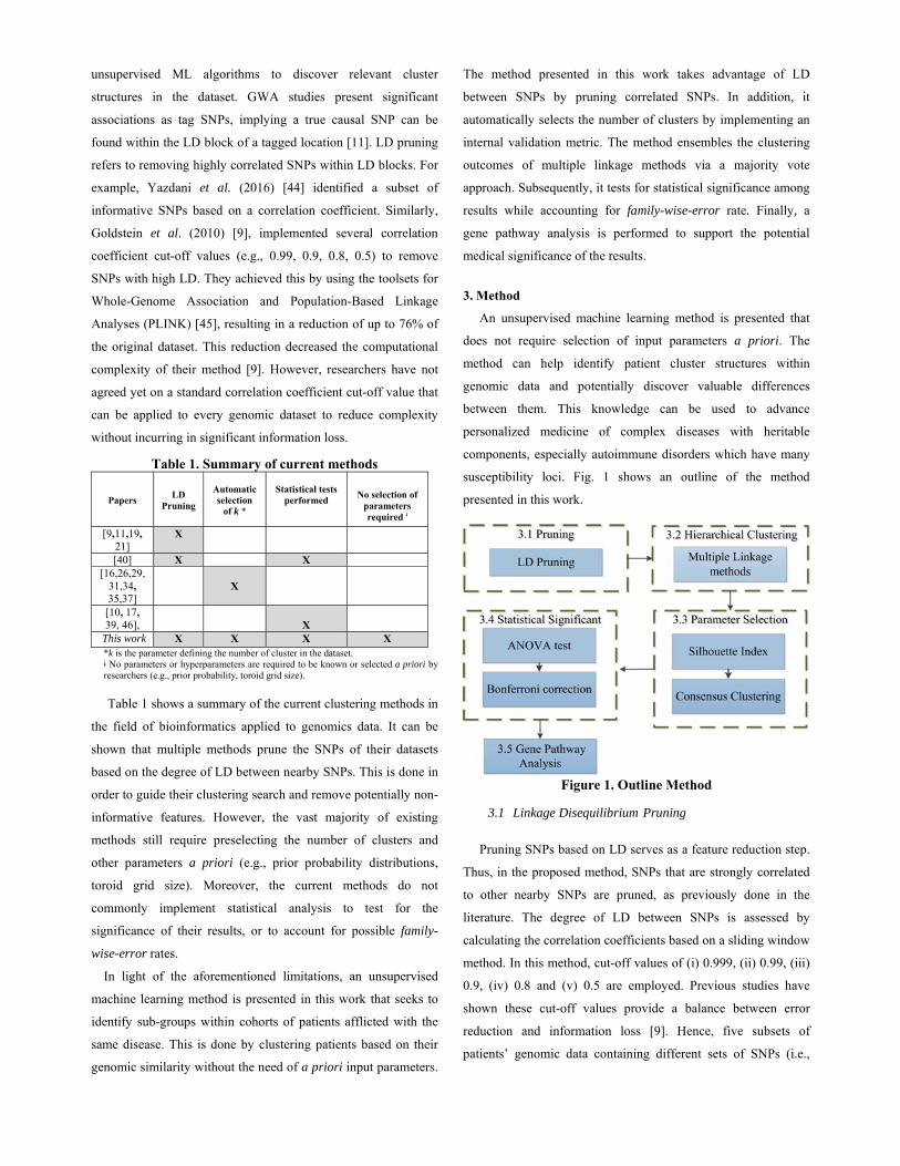
3. Method

An unsupervised machine learning method is presented that

does not require selection of input parameters a priori. The

method can help identify patient cluster structures within

genomic data and potentially discover valuable differences

between them. This knowledge can be used to advance

personalized medicine of complex diseases with heritable

components, especially autoimmune disorders which have many

susceptibility loci. Fig. 1 shows an outline of the method

presented in this work.

Figure 1. Outline Method

3.1 Linkage Disequilibrium Pruning

Pruning SNPs based on LD serves as a feature reduction step.

Thus, in the proposed method, SNPs that are strongly correlated

to other nearby SNPs are pruned, as previously done in the

literature. The degree of LD between SNPs is assessed by

calculating the correlation coefficients based on a sliding window

method. In this method, cut-off values of (i) 0.999, (ii) 0.99, (iii)

0.9, (iv) 0.8 and (v) 0.5 are employed. Previous studies have

shown these cut-off values provide a balance between error

reduction and information loss [9]. Hence, five subsets of

patients’ genomic data containing different sets of SNPs (i.e.,

features) are generated. The subsets generated serve as input for

the hierarchical clustering step.

3.2 Hierarchical Clustering

The objective of the unsupervised machine learning method

presented in this work is to cluster patients based on their

genomic similarity. Patients’ genomic similarity can be evaluated

using a wide range of distance metrics [26]. The selection of the

appropriate distance metric is driven by the type of data under

analysis (e.g., ratio, interval, ordinal, nominal or binary scale).

For example, the Euclidian distance is appropriated for ratio or

interval scale data, while the Manhattan distance for ordinal scale

data [47]. Subsequently, the method presented in this work employs an

agglomerative hierarchical clustering algorithm. Hierarchical

clustering algorithms are frequently used with only one linkage

method, which can limit their ability to identify underlying

cluster structures in certain datasets [24]. Hence, in this work,

multiple linkage methods are implemented. The linkage methods

used in this work have been shown to consistently outperform

other methods when tested with simulated GWAS datasets [26].

The cluster results obtained by implementing different linkage

methods are ensemble in the subsequent steps. This ensemble

takes advantage of the performance of multiple linkage methods.

Moreover, it helps identify the underlying structure of the data,

since the ensemble approach will favor cluster structures

identified by the majority (i.e., via a majority vote approach) of

the linkage methods. Specifically, the authors propose to

implement:

(i) Single Linkage (or Minimum Linkage).

(ii) Complete Linkage (or Maximum Linkage).

(iii) Average Linkage (or Unweighted Pair Group Method

with Arithmetic Mean, UPGMA).

(iv) Ward’s Linkage.

(v) McQuitty Linkage (or Weighted Pair Group Method

with Arithmetic Mean, WPGMA).

3.3 Parameter Selection

Once the agglomerative hierarchical algorithm is implemented,

the Silhouette index is employed as an internal validity metric.

This index has been used in previous studies to rank the results of

multiple clustering algorithms outcomes and guide the selection

of final clusters [16],[26]. Nonetheless, in this method, the index

is used to select the number of clusters for all combinations of

LD pruning data subsets (see section 3.1) and linkage methods

(see section 3.2). The number of clusters that provides the largest

average Silhouette index value in each of the combinations is

selected.

The computational complexity of testing all possible numbers

of clusters increases linearly as the number of objects in a dataset

increases. This can be a challenge in datasets that contain a large

number of objects, even with parallelized computing. In this

work, an optimization approach is presented to identify the

number of clusters that maximizes the average Silhouette index.

The mathematical formulation of this optimization problem is as

follows:

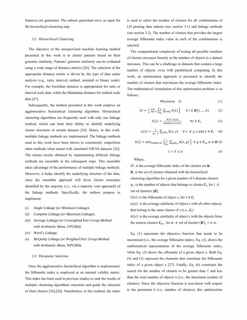
𝑀𝑎𝑥𝑖𝑚𝑖𝑧𝑒 𝑆𝐼 (1)

𝑆𝐼 ∑ ∑ 𝑆 𝑥∈𝑪 ∀ 𝑖 ∈ 𝑲 1, … , 𝑘 (2)

𝑆 𝑥 ,

∀𝑥 ∈ 𝑪 (3)

𝑎 𝑥 ∑ 𝑑 𝑥, 𝑦∈𝑪 ∀ 𝑥 𝑦, 𝑥 and 𝑦 ∈ 𝑪 (4)

𝑏 𝑖 𝑚𝑖𝑛 ∈𝑲, ∑ 𝑑 𝑥, 𝑔∈𝑪 ∀ 𝑔 ∈ 𝑪 , 𝑤 ∈ 𝑲 (5)

1 𝑘 𝑛 (6)

Where,

𝑆𝐼: is the average Silhouette index of the clusters set K

K: is the set of clusters obtained with the hierarchical

clustering algorithm for a given number of k disjoint clusters

𝜂 : is the number of objects that belongs to cluster 𝐂 , for 𝑖 ∈

𝑠et of clusters 𝑲

𝑆 𝑥 : is the Silhouette of object x, for x ∈ 𝐂

𝑎 𝑥 : is the average similarity of object x with all other objects

that belong to the same cluster of x (i.e., 𝐂 )

𝑏 𝑥 : is the average similarity of object x with the objects from

the nearest clusters 𝐂 , for 𝑤 ∈ 𝑠et of cluster 𝑲 , 𝑖 𝑤.

Eq. (1) represents the objective function that needs to be

maximized (i.e., the average Silhouette index). Eq. (2), shows the

mathematical representation of the average Silhouette index,

while Eq. (3) shows the silhouette of a given object x. Both Eq.

(4) and (5) represent the elements that constitute the Silhouette

index of a given object x [27]. Finally, Eq. (6) constrains the

search for the number of clusters to be greater than 1 and less

than the total number of objects n (i.e., the maximum number of

clusters). Since the objective function is non-linear with respect

to the parameter k (i.e., number of clusters), this optimization

problem needs to be solved with a non-linear optimization

algorithm. In the literature, there are several algorithms suitable

to solve this type of optimization problem [48]. Nonetheless, the

method is not constrained to any specific optimization algorithm.

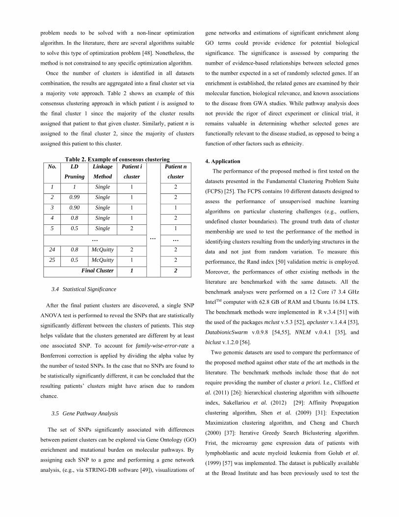
Once the number of clusters is identified in all datasets

combination, the results are aggregated into a final cluster set via

a majority vote approach. Table 2 shows an example of this

consensus clustering approach in which patient i is assigned to

the final cluster 1 since the majority of the cluster results

assigned that patient to that given cluster. Similarly, patient n is

assigned to the final cluster 2, since the majority of clusters

assigned this patient to this cluster.

Table 2. Example of consensus clustering No. LD

Pruning

Linkage

Method

Patient i

cluster

…

Patient n

cluster

1 1 Single 1 2

2 0.99 Single 1 2

3 0.90 Single 1 1

4 0.8 Single 1 2

5 0.5 Single 2 1

… …

24 0.8 McQuitty 2 2

25 0.5 McQuitty 1 2

Final Cluster 1 2

3.4 Statistical Significance

After the final patient clusters are discovered, a single SNP

ANOVA test is performed to reveal the SNPs that are statistically

significantly different between the clusters of patients. This step

helps validate that the clusters generated are different by at least

one associated SNP. To account for family-wise-error-rate a

Bonferroni correction is applied by dividing the alpha value by

the number of tested SNPs. In the case that no SNPs are found to

be statistically significantly different, it can be concluded that the

resulting patients’ clusters might have arisen due to random

chance.

3.5 Gene Pathway Analysis

The set of SNPs significantly associated with differences

between patient clusters can be explored via Gene Ontology (GO)

enrichment and mutational burden on molecular pathways. By

assigning each SNP to a gene and performing a gene network

analysis, (e.g., via STRING-DB software [49]), visualizations of

gene networks and estimations of significant enrichment along

GO terms could provide evidence for potential biological

significance. The significance is assessed by comparing the

number of evidence-based relationships between selected genes

to the number expected in a set of randomly selected genes. If an

enrichment is established, the related genes are examined by their

molecular function, biological relevance, and known associations

to the disease from GWA studies. While pathway analysis does

not provide the rigor of direct experiment or clinical trial, it

remains valuable in determining whether selected genes are

functionally relevant to the disease studied, as opposed to being a

function of other factors such as ethnicity.

4. Application

The performance of the proposed method is first tested on the

datasets presented in the Fundamental Clustering Problem Suite

(FCPS) [25]. The FCPS contains 10 different datasets designed to

assess the performance of unsupervised machine learning

algorithms on particular clustering challenges (e.g., outliers,

undefined cluster boundaries). The ground truth data of cluster

membership are used to test the performance of the method in

identifying clusters resulting from the underlying structures in the

data and not just from random variation. To measure this

performance, the Rand index [50] validation metric is employed.

Moreover, the performances of other existing methods in the

literature are benchmarked with the same datasets. All the

benchmark analyses were performed on a 12 Core i7 3.4 GHz

IntelTM computer with 62.8 GB of RAM and Ubuntu 16.04 LTS.

The benchmark methods were implemented in R v.3.4 [51] with

the used of the packages mclust v.5.3 [52], apcluster v.1.4.4 [53],

DatabionicSwarm v.0.9.8 [54,55], NNLM v.0.4.1 [35], and

biclust v.1.2.0 [56].

Two genomic datasets are used to compare the performance of

the proposed method against other state of the art methods in the

literature. The benchmark methods include those that do not

require providing the number of cluster a priori. I.e., Clifford et

al. (2011) [26]: hierarchical clustering algorithm with silhouette

index, Sakellariou et al. (2012) [29]: Affinity Propagation

clustering algorithm, Shen et al. (2009) [31]: Expectation

Maximization clustering algorithm, and Cheng and Church

(2000) [37]: Iterative Greedy Search Biclustering algorithm.

Frist, the microarray gene expression data of patients with

lymphoblastic and acute myeloid leukemia from Golub et al.

(1999) [57] was implemented. The dataset is publically available

at the Broad Institute and has been previously used to test the

performance of clustering algorithms [23,58]. The dataset is

composed of microarray gene expression data of 999 genes for

27 patients with acute lymphoblastic leukemia and 11 patients

with acute myeloid leukemia.

Lastly, a dataset of patients diagnosed with Multiple Sclerosis

(MS) is employed. DNA samples from 191 MS patients

consented via the Pennsylvania State University PRIDE protocol

at Hershey Medical Center were subjected to the Immunochip

assay (Illumina). Allelic variations were measured at previously

described susceptibility loci for multiple immune-mediated

disorders [59,60]. The Y chromosome data were filtered out of

the dataset to simplify comparisons in a predominantly female

cohort. Mitochondrial markers were discarded for analysis as

well. Genotype calling was done with Illumina GenomeStudio

v.2011.1 (www.illumina.com), and genotype markers were

excluded if their GenTrain score was less than 0.8, or if their call

rate across the cohort was less than 0.99. Finally, the MS dataset

was filtered such that only variants within coding regions (i.e.,

exons), were considered. Therefore, the MS dataset was

composed of 191 patients and 25,482 SNPs.

With the MS dataset, a 10-fold cross-validation analysis was

performed with the objective to test the performance of the

proposed and the benchmark methods, as well as to provide

evidence regarding their propensity of overfitting genomic

datasets. In this cross-validation approach, the MS dataset was

randomly partitioned into 10 subsets. Subsequently, the methods

were used to cluster the patients within these subsets. The

clustering results obtained from the 10 subsets were compared to

those from the complete dataset. The agreement between the

clusters generated with the complete MS dataset and the 10-fold

subsets is assessed with the Rand index metric. A match between

the clustering results (e.g., average Rand index of 1) will indicate

that the method was not overfitting the MS dataset, thus,

providing arguments of its generalizability. Moreover, it will

support that the method was identifying clusters due to

underlying structures in the data and not just due to random

variations. Finally, the groups of SNPs identified by the proposed

method to achieve statistical significance between clusters

generated were examined via gene pathway analysis.

4.1 Linkage Disequilibrium Pruning

For the MS dataset, the pruning of SNPs with a high LD was

done based on the correlation-coefficient cut-off values found in

the literature, as proposed in section 3.1. LD pruning was

performed using the widely used genotype analysis toolset for

Whole-Genome Association and Population-Based Linkage

Analyses (i.e., PLINK) [45]. This pruning resulted in a reduction

of the original dataset as presented in Table 3. These percentages

of SNPs removed are consistent with the results found in

previous studies.

Table 3. LD Pruning summary R2 cut-

off value Number of

SNPs retained Percentage of SNPs removed

0.50 5,460 78.57%

0.80 6,849 73.12%

0.90 7,421 70.88%

0.99 8,666 65.99%

0.999 8,691 65.89%

4.2 Hierarchical Clustering

The FCPS and Golub et al. (1999) [57] datasets contain

features that are in ratio scale. Hence, to measure the similarity

between the objects in the datasets, the Euclidian distance is

implemented. Genotype data can be ordinal or additive scale,

depending on whether heterozygous SNPs are treated as a label

or as a half-dosage. While additive models are more often used

for GWA studies, in this work, ordinal scale was used to

demonstrate flexibility in the described clustering method. Hence,

the genomic similarity of MS patients based on different subsets

of pruned data is evaluated using the Manhattan distance metric.

The similarity calculations and the agglomerative hierarchical

algorithm with multiple linkage methods were performed in R

v.3.4 [51].

4.3 Parameter Selection

The selection of the number of clusters k that maximized the

average Silhouette index was performed with a generalized

simulation annealing algorithm. This algorithm was selected due

to its underlying theory and proven performance in problems

with non-linear objective functions [61,62]. The algorithm was

implemented via the R package GenSA v.1.1.6 [63].

Nonetheless, other non-linear optimization algorithms or greedy

heuristics can also be implemented. Once the number of clusters

in every combination of LD pruned data and linkage method are

selected, the clustering results are ensemble via a majority vote

approach (see section 3.3).

4.4. Statistical Significance

After the final clusters have been selected based on the

average Silhouette metric and consensus clustering approach the

statistical significance of the results is evaluated. Clusters’

median values for each of the p features in the MS dataset are

evaluated via a single SNP non-parametric ANOVA Kruskal-

Wallis test [46]. To account for family-wise-error rate, a

Bonferroni correction is applied to the significance alpha level of

0.05 (i.e., Bonferroni correction= 0.05/p, for p= 25,482).

4.5. Gene Pathway Analysis

Gene variants that show statistical significance are further

analyzed via a gene pathway analysis to explore their potential

medical significance. Pathway analysis starts with generating a

list of genes determined from the set of SNPs with strong

evidence of significance between patient clusters. Inputting the

gene set via the STRING-DB software algorithms [49] allows for

convenient calculation of pathway enrichment hypothesis tests

and visualization of the gene network. STRING-DB determines

gene relationships by aggregating several databases into an

evidence score. Experimental evidence comes from the BIND

[64], GRID [65], HPRD [66], IntAct [67], MINT [68], and PID

[69] databases. In addition, STRING-DB pulls from the curated

databases KEGG [70], Gene Ontology [43], BioCarta [71], and

Reactome [72]. Interaction frequency is tested for enrichment

compared to expectation from a random sampling of genes, with

p-values and false discovery rates reported for enrichment in

specific cellular processes, defined by Gene Ontology references.

After statistical testing is done, the gene network is used as a

threshold for high confidence interaction and a k-means

clustering algorithm is performed for visualization purposes (see

Fig. 6).

5. Results

5.1. FCPS Benchmark results

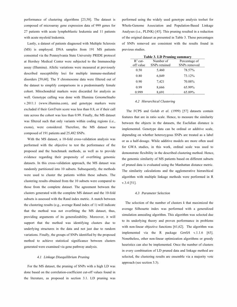
The majority of existing methods in the literature require the

selection of parameters a priori (e.g., number of clusters, see

Table 1). Hence, to benchmark with multiple methods, the

number of clusters provided by the FCPS was used as input when

testing these methods. Figure 2 shows the average Rand index

obtained in the FCPS datasets by the method proposed in this

work (i.e., Proposed) and the methods benchmarked. This plot

shows that on average the proposed method outperformed other

methods, with an average Rand index of 0.852. The performance

is statistically significantly greater than the results of the methods

proposed by Cheng and Church (2000), Sakellariou et al. (2012),

Lee and Seung (2001), Ultsch and Lötsch (2017), and Clifford et

al. (2011). Even though these results indicate that, on average,

the proposed method achieved the largest Rand index, there is

not enough evidence to conclude that it was statically

significantly greater than the Rand index achieved by the

methods of Shen et al. (2009), Hamid et al. (2010), or Ahmad et

al. (2016), at an alpha level of 0.05. This can be attributed to the

relatively small group of validation datasets provided in the

FCPS (i.e., 10 datasets).

Note: p-value: <0.001***, <0.01**, <0.05*

Figure 2. Average Rand index for FCPS datasets

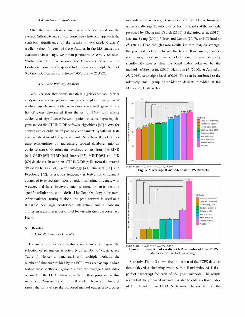
Note: p-value: <0.001***, <0.01**, <0.05*

Figure 3. Proportion of results with Rand index of 1 for FCPS datasets (i.e., perfect clustering)

Similarly, Figure 3 shows the proportion of the FCPS datasets

that achieved a clustering result with a Rand index of 1 (i.e.,

perfect clustering) for each of the given methods. The results

reveal that the proposed method was able to obtain a Rand index

of 1 in 6 out of the 10 FCPS datasets. The results from the

Wilcoxon tests indicate that these results are statistically

significantly greater than the results of the methods proposed by

Ultsch and Lötsch (2017), Cheng and Church (2000), Lee and

Seung (2001), and Sakellariou et al. (2012). Even though the

results indicate the proposed method correctly clusters the largest

percentages of datasets (i.e., 6/10), there is not enough evidence

to conclude that this proportion is statically significantly greater

than the ones from the other methods benchmarked, at an alpha

level of 0.05. Nevertheless, these results provide evidence that

the method presented in this work is able to identify true clusters

in a wider range of datasets with different underlying structures.

5.2. Genomic dataset Benchmark results

Figure 4 presents the Rand index obtained on the Golub et al.

(1999) dataset [57] by the method proposed in this work and the

benchmark methods that do not require providing the number of

clusters a priori. Fig. 4 indicates that the proposed method

performed better than the methods presented by Clifford et al.

(2011), Cheng and Church (2000), and Sakellariou et al. (2012).

Figure 4. Rand index for Leukemia dataset

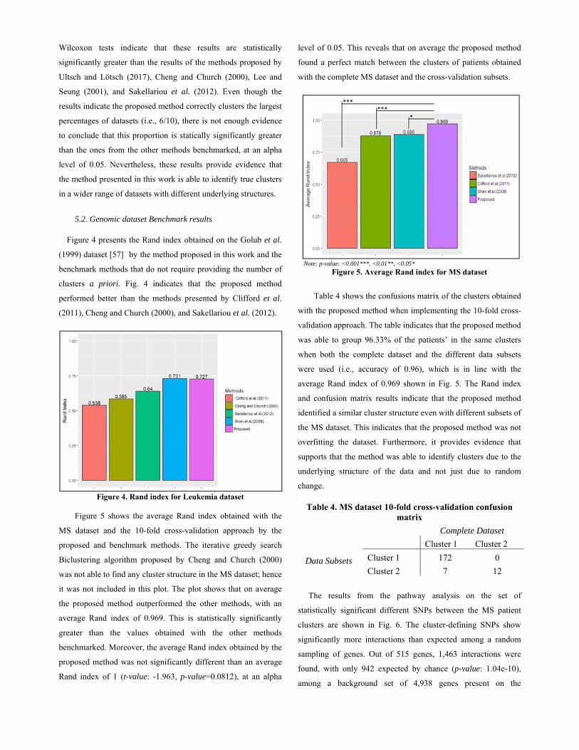
Figure 5 shows the average Rand index obtained with the

MS dataset and the 10-fold cross-validation approach by the

proposed and benchmark methods. The iterative greedy search

Biclustering algorithm proposed by Cheng and Church (2000)

was not able to find any cluster structure in the MS dataset; hence

it was not included in this plot. The plot shows that on average

the proposed method outperformed the other methods, with an

average Rand index of 0.969. This is statistically significantly

greater than the values obtained with the other methods

benchmarked. Moreover, the average Rand index obtained by the

proposed method was not significantly different than an average

Rand index of 1 (t-value: -1.963, p-value=0.0812), at an alpha

level of 0.05. This reveals that on average the proposed method

found a perfect match between the clusters of patients obtained

with the complete MS dataset and the cross-validation subsets.

\Note: p-value: <0.001***, <0.01**, <0.05* Figure 5. Average Rand index for MS dataset

Table 4 shows the confusions matrix of the clusters obtained

with the proposed method when implementing the 10-fold cross-

validation approach. The table indicates that the proposed method

was able to group 96.33% of the patients’ in the same clusters

when both the complete dataset and the different data subsets

were used (i.e., accuracy of 0.96), which is in line with the

average Rand index of 0.969 shown in Fig. 5. The Rand index

and confusion matrix results indicate that the proposed method

identified a similar cluster structure even with different subsets of

the MS dataset. This indicates that the proposed method was not

overfitting the dataset. Furthermore, it provides evidence that

supports that the method was able to identify clusters due to the

underlying structure of the data and not just due to random

change.

Table 4. MS dataset 10-fold cross-validation confusion matrix

Complete Dataset

Cluster 1 Cluster 2

Data Subsets

Cluster 1 172 0

Cluster 2 7 12

The results from the pathway analysis on the set of

statistically significant different SNPs between the MS patient

clusters are shown in Fig. 6. The cluster-defining SNPs show

significantly more interactions than expected among a random

sampling of genes. Out of 515 genes, 1,463 interactions were

found, with only 942 expected by chance (p-value: 1.04e-10),

among a background set of 4,938 genes present on the

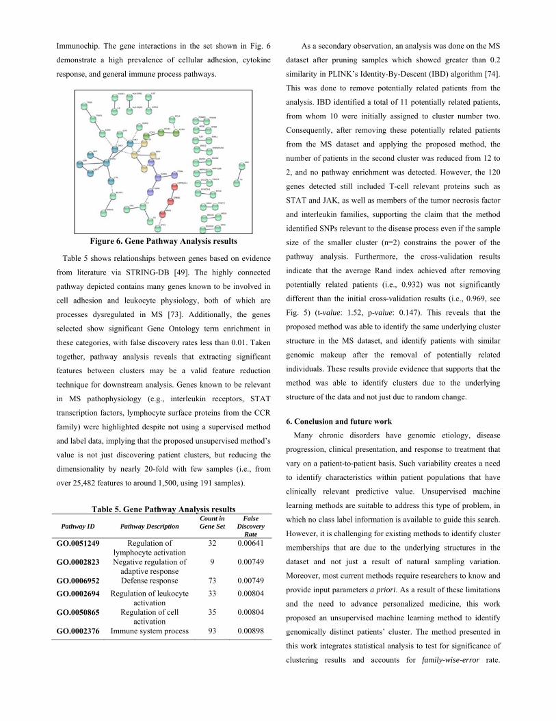
Immunochip. The gene interactions in the set shown in Fig. 6

demonstrate a high prevalence of cellular adhesion, cytokine

response, and general immune process pathways.

Figure 6. Gene Pathway Analysis results Table 5 shows relationships between genes based on evidence

from literature via STRING-DB [49]. The highly connected

pathway depicted contains many genes known to be involved in

cell adhesion and leukocyte physiology, both of which are

processes dysregulated in MS [73]. Additionally, the genes

selected show significant Gene Ontology term enrichment in

these categories, with false discovery rates less than 0.01. Taken

together, pathway analysis reveals that extracting significant

features between clusters may be a valid feature reduction

technique for downstream analysis. Genes known to be relevant

in MS pathophysiology (e.g., interleukin receptors, STAT

transcription factors, lymphocyte surface proteins from the CCR

family) were highlighted despite not using a supervised method

and label data, implying that the proposed unsupervised method’s

value is not just discovering patient clusters, but reducing the

dimensionality by nearly 20-fold with few samples (i.e., from

over 25,482 features to around 1,500, using 191 samples).

Table 5. Gene Pathway Analysis results

Pathway ID

Pathway Description

Count in Gene Set

False Discovery

Rate

GO.0051249 Regulation of lymphocyte activation

32 0.00641

GO.0002823 Negative regulation of adaptive response

9 0.00749

GO.0006952 Defense response 73 0.00749

GO.0002694 Regulation of leukocyte activation

33 0.00804

GO.0050865 Regulation of cell activation

35 0.00804

GO.0002376 Immune system process 93 0.00898

As a secondary observation, an analysis was done on the MS

dataset after pruning samples which showed greater than 0.2

similarity in PLINK’s Identity-By-Descent (IBD) algorithm [74].

This was done to remove potentially related patients from the

analysis. IBD identified a total of 11 potentially related patients,

from whom 10 were initially assigned to cluster number two.

Consequently, after removing these potentially related patients

from the MS dataset and applying the proposed method, the

number of patients in the second cluster was reduced from 12 to

2, and no pathway enrichment was detected. However, the 120

genes detected still included T-cell relevant proteins such as

STAT and JAK, as well as members of the tumor necrosis factor

and interleukin families, supporting the claim that the method

identified SNPs relevant to the disease process even if the sample

size of the smaller cluster (n=2) constrains the power of the

pathway analysis. Furthermore, the cross-validation results

indicate that the average Rand index achieved after removing

potentially related patients (i.e., 0.932) was not significantly

different than the initial cross-validation results (i.e., 0.969, see

Fig. 5) (t-value: 1.52, p-value: 0.147). This reveals that the

proposed method was able to identify the same underlying cluster

structure in the MS dataset, and identify patients with similar

genomic makeup after the removal of potentially related

individuals. These results provide evidence that supports that the

method was able to identify clusters due to the underlying

structure of the data and not just due to random change.

6. Conclusion and future work

Many chronic disorders have genomic etiology, disease

progression, clinical presentation, and response to treatment that

vary on a patient-to-patient basis. Such variability creates a need

to identify characteristics within patient populations that have

clinically relevant predictive value. Unsupervised machine

learning methods are suitable to address this type of problem, in

which no class label information is available to guide this search.

However, it is challenging for existing methods to identify cluster

memberships that are due to the underlying structures in the

dataset and not just a result of natural sampling variation.

Moreover, most current methods require researchers to know and

provide input parameters a priori. As a result of these limitations

and the need to advance personalized medicine, this work

proposed an unsupervised machine learning method to identify

genomically distinct patients’ cluster. The method presented in

this work integrates statistical analysis to test for significance of

clustering results and accounts for family-wise-error rate.

Moreover, the method is capable of automatically identifying the

number of clusters by implementing an internal validity metric.

Similarly, the method takes advantage of the degree of linkage

disequilibrium between SNPs by pruning correlated nearby SNPs,

as well as implementing a post-clustering gene pathways analysis.

The method is tested with clustering validation datasets

previously used in the literature. The benchmark results reveal

that proposed method provides, on average, the greatest

performance (i.e., average Rand index 0.852). Moreover, results

indicate that it was able to obtain cluster results with a Rand

index of 1 (i.e., perfect clustering) in 6 out of the 10 Fundamental

Clustering Problem Suite datasets. Similarly, the method is

applied to a dataset of 38 patients with leukemia, and

subsequently to a dataset of 191 Multiple Sclerosis (MS) patients.

The results indicate that the method is able to identify genetically

distinct patient clusters without the need to select the number of

clusters or any input parameter a priori. Moreover, the cross-

validation results indicate that the method presented in this work

outperformed the other methods found in the literature when it

comes to data overfitting, since the average Rand index obtained

was significantly greater than the benchmarked methods and not

significantly different than 1. This performance was maintained

even after the removal of potentially related patients from the

dataset. This indicates that the method was identifying clusters

due to the underlying structure of the data and avoided overfitting

the dataset. The identification of distinct genetic subtypes of

patients demonstrates the potential applicability of this process to

advance personalized medicine of complex diseases with

heritable components, especially autoimmune disorders.

When applied to genomic data, the method also shows value

as a feature reduction strategy. Out of over 25,482 exonic SNPs

and 191 patient samples, the clustering of patients yielded a set of

SNPs which significantly vary between clusters. These variants

represent 515 genes, several of which are known to be involved

in MS (CD69, CCRX5, IL-13, STAT3) and cell adhesion

(ICAM1, LAMB4). The fact that many highlighted genes are

components of the immune system is not surprising due to the

nature of the Immunochip assay, but the enrichment of

leukocyte-specific genes is evidence that the method can result in

functionally relevant feature sets, even without class labels.

Notably, 57 genes representing over 10% of the network are

involved in cytokine receptor processes. This is greater than

expected from random chance, as cytokine receptors constitute a

small percentage of all Immunochip genes. The evidence

presented in this work alone is insufficient to define genetic

subtypes of MS, but the specific SNP set reaching significance

may be a valuable resource in experimental studies examining

immune cell dynamics and genetics. For example, the hypothesis

that these clusters represent different subtypes of MS, can be

tested by evaluating clinical criteria such as image results and

disease progression, as well as quantitative cytokine profiling and

gene expression studies for each cluster, compared against

random groupings of patients.

This work demonstrates an iterative unsupervised machine

learning method which identifies significant patient clusters

within a genomic dataset. Future research should explore the

medical significance of the findings shown in this work.

Similarly, the method from this work should be implemented in

studies collecting SNP array and gene expression microarray data

from additional disease cohorts to explore its potential benefits.

Further investigation can extend beyond pathway analysis to

evaluate these clusters for clinical significance of genetically

related characteristics such as age of onset, disease course,

heritability, and response to treatment. Once links are drawn

between clusters and clinically relevant outcomes, the

Immunochip can be used to classify high-risk and newly

diagnosed chronic disease patients into clusters with predictive

value.

Acknowledgments

The authors acknowledge the NSF I/UCRC Center for

Healthcare Organization Transformation (CHOT), NSF I/UCRC

grant #1624727, and the Institute for Personalized Medicine at

the Pennsylvania State University. Additionally, the authors

would like to acknowledge Dr. James R. Broach from the

Institute for Personalized Medicine at the Pennsylvania State

University, for his valuable contributions. Any opinions,

findings, or conclusions found in this paper are those of the

authors and do not necessarily reflect the views of the sponsors.

References

[1] M.K.K. Leung, A. Delong, B. Alipanahi, B.J. Frey, Machine Learning in Genomic Medicine: A Review of Computational Problems and Data Sets, Proceedings of the IEEE. 104 (2016) 176–197. doi:10.1109/JPROC.2015.2494198.

[2] M.W. Libbrecht, W.S. Noble, Machine learning in genetics and genomics, Nature Reviews. Genetics. 16 (2015) 321–332. doi:10.1038/nrg3920.Machine.

[3] R. Upstill-Goddard, D. Eccles, J. Fliege, A. Collins, Machine learning approaches for the discovery of gene-gene interactions in disease data, Briefings in

Bioinformatics. 14 (2013) 251–260. doi:10.1093/bib/bbs024.

[4] K.Y. Yip, C. Cheng, M. Gerstein, Machine learning and genome annotation: a match meant to be?, Genome Biology. 14 (2013) 205. doi:10.1186/gb-2013-14-5-205.

[5] C.J. Ross, F. Towfic, J. Shankar, D. Laifenfeld, M. Thoma, M. Davis, B. Weiner, R. Kusko, B. Zeskind, V. Knappertz, I. Grossman, M.R. Hayden, A pharmacogenetic signature of high response to Copaxone in late-phase clinical-trial cohorts of multiple sclerosis, Genome Medicine. 9 (2017). doi:10.1186/s13073-017-0436-y.

[6] O. Kulakova, E. Tsareva, D. Lvovs, A. Favorov, A. Boyko, O. Favorova, Comparative pharmacogenetics of multiple sclerosis: INF-B versus glatiramer acetate, Pharmacogenomics. 15 (2014) 679–85.

[7] W. Xu, L. Zhang, Y. Lu, SD-MSAEs: Promoter recognition in human genome based on deep feature extraction, Journal of Biomedical Informatics. 61 (2016) 55–62. doi:10.1016/j.jbi.2016.03.018.

[8] Y. Zhao, B.C. Healy, D. Rotstein, C.R.G. Guttmann, R. Bakshi, H.L. Weiner, C.E. Brodley, T. Chitnis, Exploration of machine learning techniques in predicting multiple sclerosis disease course., PloS One. 12 (2017) e0174866. doi:10.1371/journal.pone.0174866.

[9] B.A. Goldstein, A.E. Hubbard, A. Cutler, L.F. Barcellos, An application of Random Forests to a genome-wide association dataset: Methodological considerations & new findings, BMC Genetics. 11 (2010) 49. doi:10.1186/1471-2156-11-49.

[10] P.K. Kimes, Y. Liu, D. Neil Hayes, J.S. Marron, Statistical significance for hierarchical clustering, Biometrics. (2017). doi:10.1111/biom.12647.

[11] K.K.-H. Farh, A. Marson, J. Zhu, M. Kleinewietfeld, W.J. Housley, S. Beik, N. Shoresh, H. Whitton, R.J.H. Ryan, A.A. Shishkin, M. Hatan, M.J. Carrasco-Alfonso, D. Mayer, C.J. Luckey, N.A. Patsopoulos, P.L. De Jager, V.K. Kuchroo, C.B. Epstein, M.J. Daly, D.A. Hafler, B.E. Bernstein, Genetic and epigenetic fine mapping of causal autoimmune disease variants, Nature. 518 (2015) 337–343. doi:10.1038/nature13835.

[12] S. Lim, C.S. Tucker, S. Kumara, An unsupervised machine learning model for discovering latent infectious diseases using social media data, J Biomed Informat. 66 (2017) 82–94.

[13] R. Xu, D.C. Wunsch, Clustering algorithms in biomedical research: A review, IEEE Reviews in Biomedical Engineering. 3 (2010) 120–154. doi:10.1109/RBME.2010.2083647.

[14] A. Prelić, S. Bleuler, P. Zimmermann, A. Wille, P. Bühlmann, W. Gruissem, E. Zitzler, A systematic comparison and evaluation of biclustering methods for gene expression data, Bioinformatics. 9 (2006) 1122–1129.

[15] A.K. Jain, M.N. Murty, P.J. Flynn, Data clustering: a review, ACM Computing Surveys. 31 (1999) 264–323. doi:10.1145/331499.331504.

[16] I.A. Pagnuco, Juan I. Pastorea;, G. Abras;, M. Brun;, V.L. Ballarin;, Analysis of genetic association using hierarchical clustering and cluster validation indices, Genomics. (2017) 4–11. doi:10.1016/j.pscychresns.2008.11.004.

[17] T. Ahmad, N. Desai, F. Wilson, P. Schulte, A. Dunning, D. Jacoby, L. Allen, M. Fiuzat, J. Rogers, G.M. Felker, Clinical implications of cluster analysis-based classification of acute decompensated heart failure and

correlation with bedside hemodynamic profiles, PloS One. 11 (2016) e0145881.

[18] K. Mei, J. Peng, L. Gao, N.N. Zheng, J. Fan, Hierarchical Classification of Large-Scale Patient Records for Automatic Treatment Stratification, IEEE Journal of Biomedical and Health Informatics. 19 (2015) 1234–1245. doi:10.1109/JBHI.2015.2414876.

[19] J.S. Hamid, C. Meaney, N.S. Crowcroft, J. Granerod, J. Beyene, Cluster analysis for identifying sub-groups and selecting potential discriminatory variables in human encephalitis., BMC Infectious Diseases. 10 (2010) 364. doi:10.1186/1471-2334-10-364.

[20] W. Redekop, D. Mladsi, The faces of personalized medicine: a framework for understanding its meaning and scope, Value in Health. 6 (2013) S4–S9.

[21] L. Tari, C. Baral, S. Kim, Fuzzy c-means clustering with prior biological knowledge, Journal of Biomedical Informatics. 42 (2009) 74–81. doi:10.1016/j.jbi.2008.05.009.

[22] R. Bellazzi, B. Zupan, Towards knowledge-based gene expression data mining, Journal of Biomedical Informatics. 40 (2007) 787–802. doi:10.1016/j.jbi.2007.06.005.

[23] C. Wiwie, J. Baumbach, R. Röttger, Comparing the performance of biomedical clustering methods, Nature Methods. 12 (2015) 1033–1038. doi:10.1038/nmeth.3583.

[24] A. Ultsch, J. Lötsch, Machine-learned cluster identification in high-dimensional data, Journal of Biomedical Informatics. 66 (2017) 95–104. doi:10.1016/j.jbi.2016.12.011.

[25] A. Ultsch, Clustering with SOM: U*C., in: In Proceedings of the 5th Workshop on Self-Organizing Maps, Paris, 2005: pp. 75–82.

[26] H. Clifford, F. Wessely, S. Pendurthi, R.D. Emes, Comparison of clustering methods for investigation of genome-wide methylation array data, Frontiers in Genetics. 2 (2011) 1–11. doi:10.3389/fgene.2011.00088.

[27] P.J. Rousseeuw, Silhouettes: A graphical aid to the interpretation and validation of cluster analysis, Journal of Computational and Applied Mathematics. 20 (1987) 53–65. doi:10.1016/0377-0427(87)90125-7.

[28] J.C. Bezdek, N.R. Pal, Some new indexes of cluster validity, IEEE Transactions on Systems, Man, and Cybernetics, Part B: Cybernetics. 28 (1998) 301–315. doi:10.1109/3477.678624.

[29] A. Sakellariou, D. Sanoudou, G. Spyrou, Combining multiple hypothesis testing and affinity propagation clustering leads to accurate, robust and sample size independent classification on gene expression data, BMC Bioinformatics. 13 (2012) 270.

[30] B.J. Frey, D. Dueck, Clustering by passing messages between data points, Science. 315 (2007) 972–976.

[31] R. Shen, A.B. Olshen, M. Ladanvi, Integrative clustering of multiple genomic data types using a joint latent variable model with application to breast and lung cancer subtype analysis, Bioinformatics. 25 (2009) 2906–2912.

[32] A.P. Dempster, N.M. Laird, D.B. Rubin, Maximum likelihood from incomplete data via the EM algorithm, J Royal Stat Soc Series B. (1977) 1–38.

[33] C. Fraley, A.E. Raftery, How many clusters? Which clustering method? Answers via model-based cluster analysis., The Comp Journal. 41 (1998) 578–588.

[34] S. Khakabimamaghani, M. Ester, Bayesian biclustering for patient stratification, Biocomputing 2016: Proceedings of the Pacific Symposium. (2016) 345–356.

[35] D. Lee, H. Seung, Algorithms for non-negative matrix factorization, Advances in Neural Information Processing Systems. (2001) 556–562.

[36] B. Pontes, R. Giráldez, J. Aguilar-Ruiz, Biclustering on expression data: A review, Journal of Biomedical Informatics. 57 (2015) 163–180.

[37] Y. Cheng, G. Church, Biclustering of expression data, Proceedings of the 8th International Conference on Intelligent Systems for Molecular Biology, La Jolla, CA. (2000) 93–103.

[38] N. Nguyen, R. Caruana, Consensus clusterings, in: Proceedings - IEEE International Conference on Data Mining, ICDM, 2007: pp. 607–612. doi:10.1109/ICDM.2007.73.

[39] R. Suzuki, H. Shimodaira, pvclust : An R package for hierarchical clustering with p-values, Bioinformatics. 22 (2013) 1–7.

[40] P.R. Bushel, H.K. Hamadeh, L. Bennett, J. Green, A. Ableson, S. Misener, C.A. Afshari, R.S. Paules, Computational selection of distinct class- and subclass-specific gene expression signatures, Journal of Biomedical Informatics. 35 (2002) 160–170. doi:10.1016/S1532-0464(02)00525-7.

[41] R.J. Cabin, R.J. Mitchell, To Bonferroni or not to Bonferroni: when and how are the questions, Bulletin of the Ecological Society of America. 81 (2000) 246–248. doi:10.2307/20168454.

[42] J.C. Bezdek, R. Ehrlich, FCM: The fuzzy c-means clustering algorithm, Comp and Geosci. 10 (1984) 191–203.

[43] M. Ashburner, C.A. Ball, J.A. Blake, D. Botstein, H. Butler, J.M. Cherry, A.P. Davis, K. Dolinski, S.S. Dwight, J.T. Eppig, M.A. Harris, D.P. Hill, L. Issel-Tarver, A. Kasarskis, S. Lewis, J.C. Matese, J.E. Richardson, M. Ringwald, G.M. Rubin, G. Sherlock, Gene Ontology: tool for the unification of biology, Nature Genetics. 25 (2000) 25–29. doi:10.1038/75556.

[44] A. Yazdani, A. Yazdani, A. Samiei, E. Boerwinkle, Generating a robust statistical causal structure over 13 cardiovascular disease risk factors using genomics data, Journal of Biomedical Informatics. 60 (2016) 114–119. doi:10.1016/j.jbi.2016.01.012.

[45] S. Purcell, B. Neale, K. Todd-Brown, L. Thomas, M.A.R. Ferreira, D. Bender, J. Maller, P. Sklar, P.I.W. de Bakker, M.J. Daly, P.C. Sham, PLINK: A Tool Set for Whole-Genome Association and Population-Based Linkage Analyses, The American Journal of Human Genetics. 81 (2007) 559–575. doi:10.1086/519795.

[46] G.P. Rédei, Kruskal-Wallis test, Encyclopedia of Genetics, Genomics, Proteomics, and Informatics. (2008) 1067–1068.

[47] B.S. Everitt, S. Landau, M. Leese, D. Stahl, Measurement of Proximity, Cluster Analysis. (2011) 43–69. doi:10.1002/9780470977811.ch3.

[48] M.S. Bazaraa, H.D. Sherali, C.M. Shetty, Nonlinear programming: theory and algorithms, John Wiley & Sons, Chicago, 2013.

[49] Szklarczyk et al, STRING v10: protein-protein interaction networks, integrated over the tree of life, Nucleic Acids Research. D1 (2015) 447–452.

[50] W.M. Rand, Objective criteria for the evaluation of clustering methods, J Amer Stat Assoc. 66 (1971) 846–50.

[51] R. R Development Core Team, R: A Language and Environment for Statistical Computing, 1 (2011).

[52] C. Fraley, A.E. Raftery, T.B. Murphy, L. Scrucca, mclust Version 4 for R: Normal Mixture Modeling for Model-

Based Clustering, Classification, and Density Estimation, Technical Report No. 597, Dept of Statistics, University of Washington. (2012).

[53] U. Bodenhofer, A. Kothmeier, S. Hochreiter, APCluster: an R package for affinity propagation clustering, Bioinformatics. 27 (2011) 2463–4.

[54] M.C. Thrun, F. Lerch, J. Lotsch, A. Ultsch, Visualization and 3D printing of multivariate data of biomarkers, in: Proceedings of International Conference in Central Europe on Computer Graphics, Visualization, and Computer Vision, Plzen, 2016.

[55] M.C. Thrun, Projection based clustering through self-organization and swarm intelligence: combining cluster analysis with the visualization of high-dimensional data., Springer Fachmedien, Wiesbaden, Germany, 2018.

[56] S. Kaiser, R. Santamaria, T. Khamiakova, M. Sill, R. Theron, L. Quintales, F. Leisch, E. DeTroyer, biclust: BiCluster Algorithms, R Package Version 1. no. 1 (2015).

[57] T. Golub, D. Slonim, P. Tamayo, C. Huard, M. Gaasenbeek, J. Mesirov, H. Coller, M. Loh, J. Downing, M. Caliguiri, C. Bloomfield, E. Lander, Molecular classification of cancer: class discovery and class prediction by gene expression monitoring, Science. 5439 (1999) 531–7.

[58] S. Monti, P. Tamayo, J. Mesirov, T. Golub, Consensus clustering: a resampling-based method for class discovery and visualization of gene expression microarray data, Machine Learning. 52 (2003) 91–118.

[59] A. Cortes, M.A. Brown, Promise and pitfalls of the Immunochip, Arthritis Research & Therapy. 13 (2011) 101.

[60] D. Welter, J. MacArthur, J. Morales, T. Burdett, P. Hall, H. Junkins, A. Klemm, P. Flicek, T. Manolio, L. Hindorff, H. Parkinson, The NHGRI GWAS Catalog, a curated resource of SNP-trait associations, Nucleic Acids Research. 42 (2014) D1001–D1006. doi:10.1093/nar/gkt1229.

[61] S. Kirkpatrick, C.D. Gelatt, M.P. Vecchi, Optimization by simulated annealing, Science. 220 (1983) 671–80.

[62] C.E. López, D. Nembhard, Cooperative workforce planning heuristic with worker learning and forgetting and demand constraints, in: IIE Annual Conference Proceedings, 2017: pp. 380–85.

[63] Y. Xiang, S. Gubian, B. Suomela, J. Hoeng, Generalized simulated annealing for global optimization: the GenSA Package, R J. 5 (2013) 13–28.

[64] G.D. Bader, D. Betel, C.W.V. Hogue, BIND: the Biomolecular Interaction Network Database, Nucleic Acids Research. 31 (2003) 248–50.

[65] A. Chatr-Aryamontri, R. Oughtred, L. Boucher, J. Rust, C. Chang, N.K. Kolas, L. O’Donnell, S. Oster, C. Theesfeld, A. Sellam, C. Stark, B.J. Breitkreutz, K. Dolinski, M. Tyers, The BioGRID interaction database: 2017 update, Nucleic Acids Research. (2016).

[66] T.S.K. Prasad et al, Human Protein Reference Database - 2009 Update, Nucleic Acids Research. (2009) D767-72.

[67] H. Hermjakob, L. Montecchi-Palazzi, C. Lewington et al, IntAct: an open source molecular interaction database, Nucleic Acids Research. (2004) D452-5.

[68] L. Licata, L. Briganti, D. Peluso, L. Perfetto, M. Iannuccelli, E. Galeota, F. Sacco, A. Palma, A.P. Nardozza, E. Santonico, L. Castagnoli, G. Cesareni, MINT, the molecular interaction database: 2012 update, Nucleic Acids Research. (2012).

[69] C.F. Schaefer, K. Anthony, S. Krupa et al, PID: the Pathway Interaction Database, Nucleic Acids Research. (2009) D674-9.

[70] Kanehisa, M. Furumichi, M. Tanabe, Y. Sato, K. Morishima, KEGG: new perspectives on genomes, pathways, diseases, and drugs, Nucleic Acids Research. (2017) D353-61.

[71] D. Nishimura, Biotech software and internet report, BioCarta, BIotech Software & Internet Report: The Computer Software Journal for Scient 2(3). (2004). https://doi.org/10.1089/152791601750294344.

[72] Fabregat et al, The reactome pathway knowledgebase, Nucleic Acids Research. D1 (2015) 481–487.

[73] C. Larochelle, J. Alvarez, W. Just, How do immune cells overcome the blood-brain barrier in multiple sclerosis?, FEBS Letters. (2012).

[74] N. Isobe, et. al., An Immunochip study of multiple sclerosis risk in African Americans, Brain. 138 (2015) 1518–30.