Embed Size (px)
Citation preview
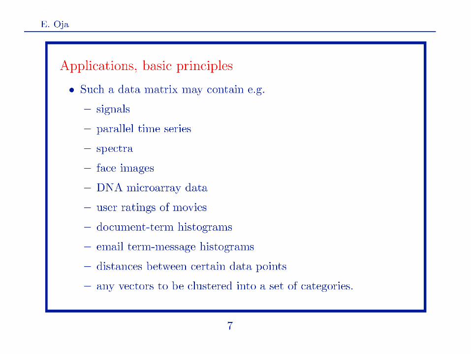
Unsupervised Machine Learning for Matrix
Decomposition
Erkki Oja
Department of Computer Science
Aalto University, Finland
Machine Learning Coffee Seminar, Monday Jan. 9, HIIT
Matrix Decomposition
• Assume three matrices A, B, and C
• Consider equation
A = BC
• If any two matrices are known, the third one
can be solved
• Very dull. So what?
• But let us consider the case when only one (say, A) is known.
• Then A BC is called a matrix decomposition for A
• This is not unique but becomes very useful when suitable constraints are posed.
• Some very promising machine learning techniques are based on this.
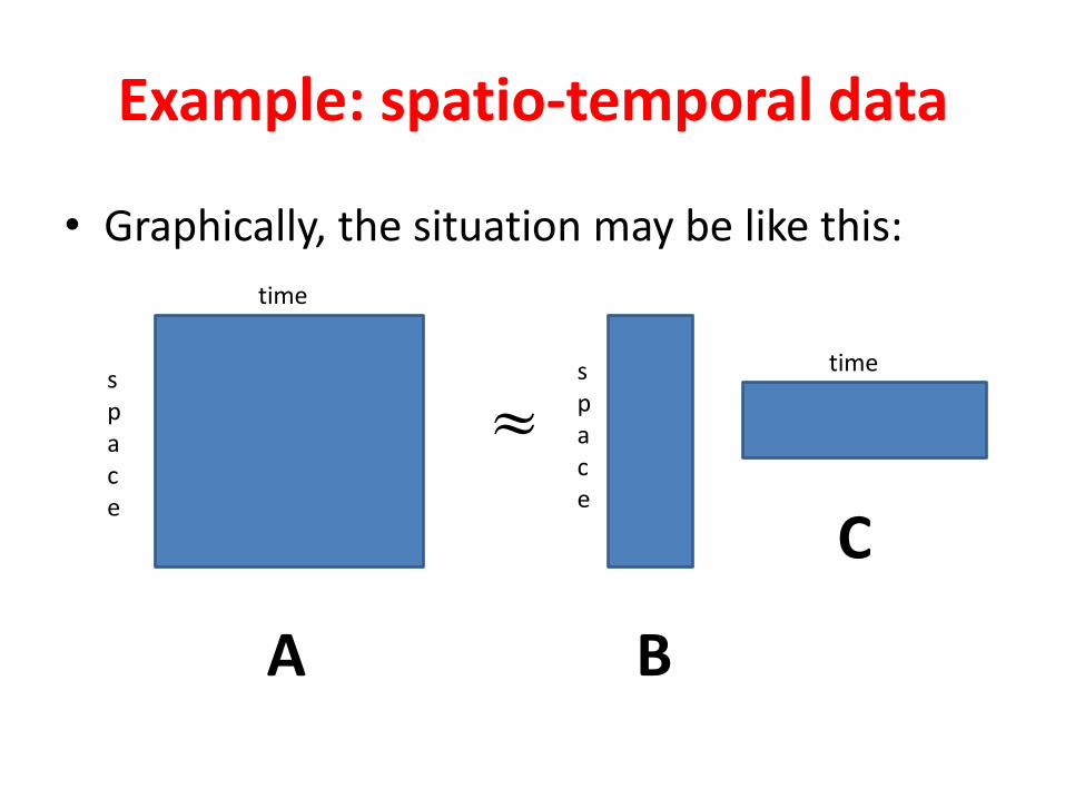
Example: spatio-temporal data
• Graphically, the situation may be like this:
space
space
time
time
A B
C
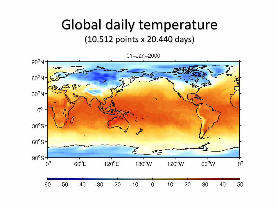
Global daily temperature (10.512 points x 20.440 days)

E.g. global warming component
One row of matrix C
Corresponding column of matrix B
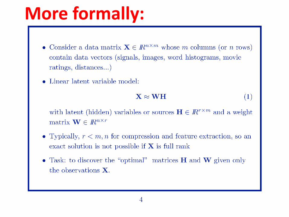
More formally:
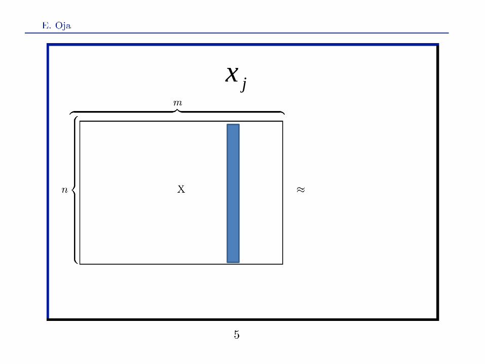
jx

ij
i
ihw
W

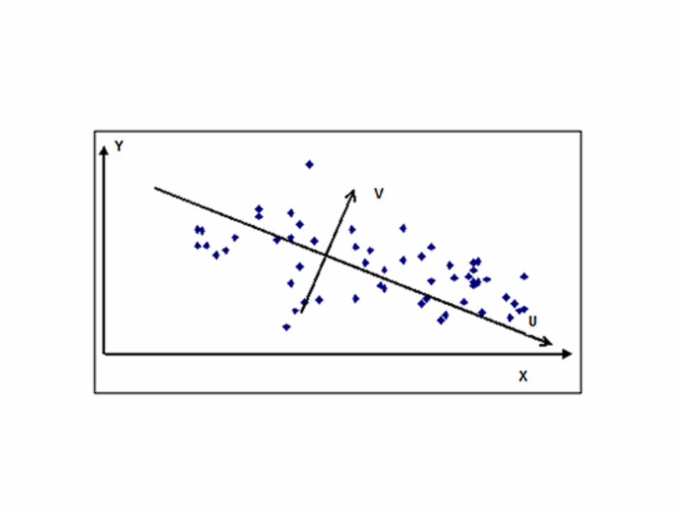
Principal Component Analysis (PCA)
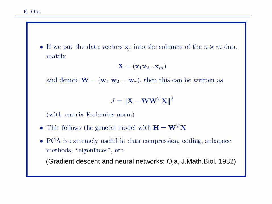
(Gradient descent and neural networks: Oja, J.Math.Biol. 1982)
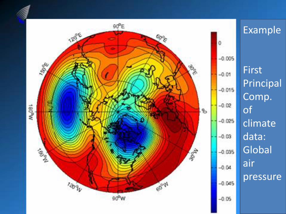
Example First Principal Comp. of climate data: Global air pressure
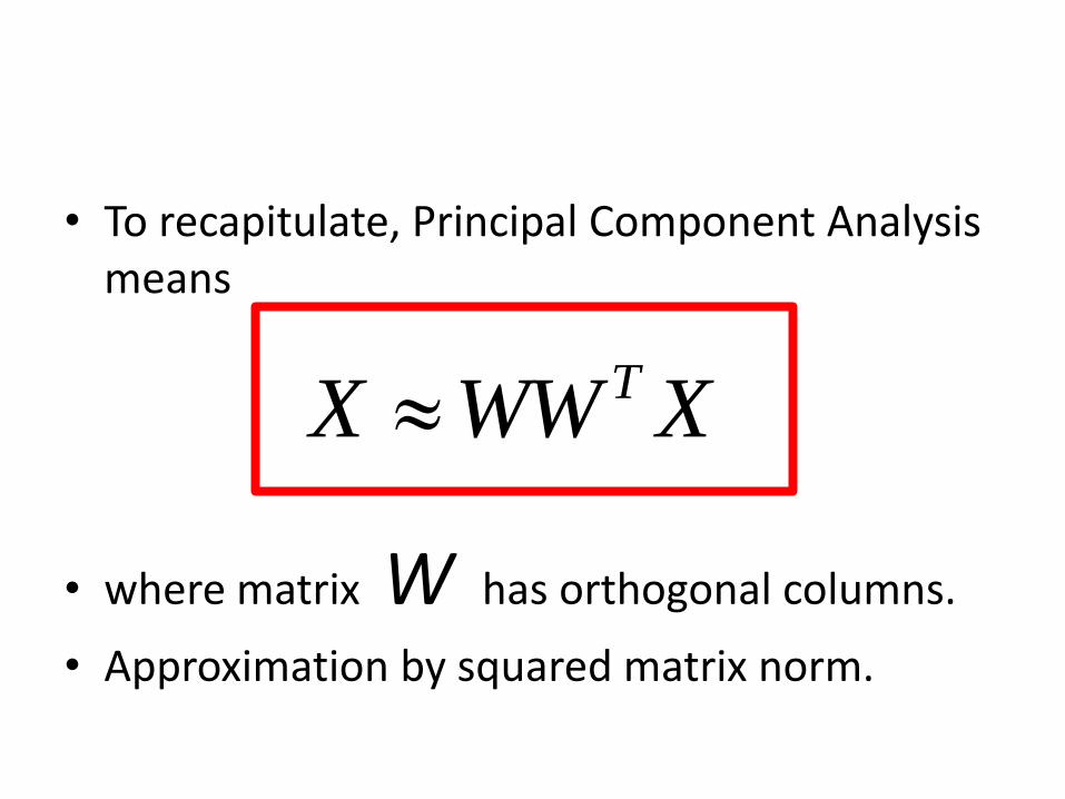
• To recapitulate, Principal Component Analysis means
• where matrix W has orthogonal columns.
• Approximation by squared matrix norm.
XWWX T
• PCA and related classical models, like factor analysis, were more or less the state-of-the-art of unsupervised machine learning for linear latent variable models 25 years ago, during the first ICANN conference.
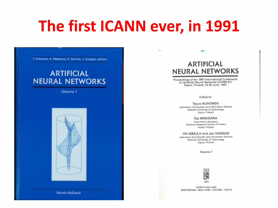
The first ICANN ever, in 1991
• My problem at that time: what is nonlinear PCA ?
• My solution: a novel neural network, deep auto-encoder
• E. Oja: Data compression, feature extraction, and auto-association in feedforward neural networks. Proc. ICANN 1991, pp. 737-745.
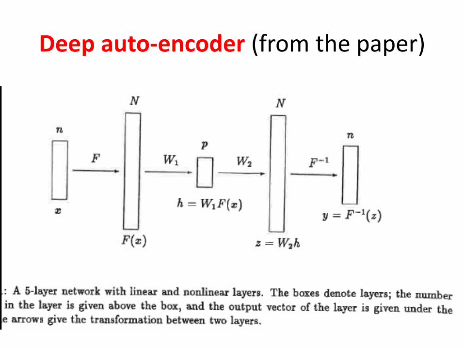
Deep auto-encoder (from the paper)
• The trick is that a data vector x is both the input and the desired output.
• This was one of the first papers on multilayer (deep) auto-encoders, which today are quite popular.
• In those days, this was quite difficult to train.
• Newer results: Hinton and Zemel (1994), Bengio (2009), and many others.

Independent Component Analysis (ICA)
• A signal processing / data-analysis technique first developed by Jutten et al (1985), Comon (1989, 1994), Cardoso (1989,1998), Amari et al (1996), Cichocki (1994), Bell and Sejnowski (1995) and many others
• Let’s just look at an example using images.
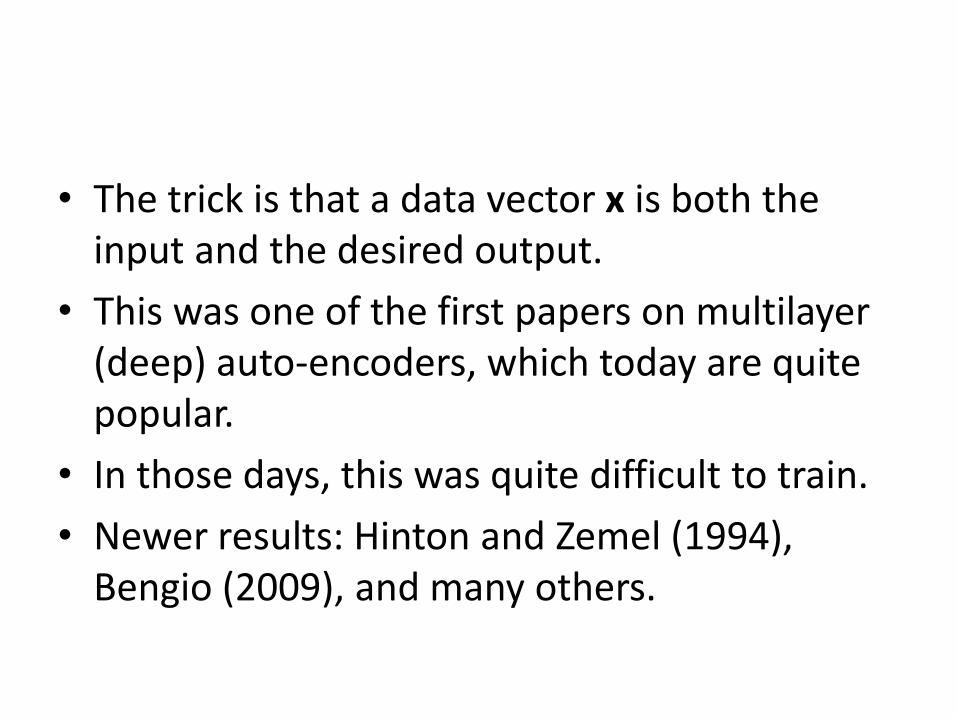
Original 9 “independent” images (rows of matrix H)
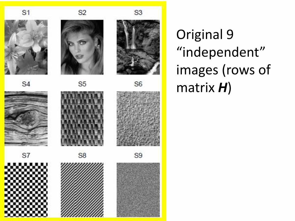
9 mixtures with random mixing matrix W; these images are the rows of matrix X, and this is the only available data we have
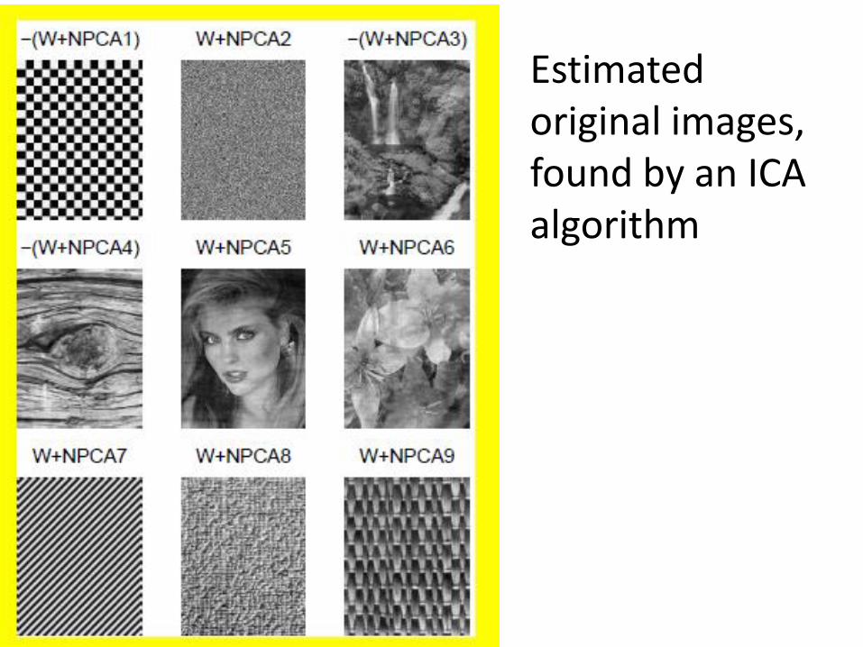
Estimated original images, found by an ICA algorithm
• Pictures are from the book “Independent Component Analysis” by Hyvärinen, Karhunen, and Oja (Wiley, 2001)
• ICA is still an active research topic: see the Int. Workshops on ICA and blind source separation / Latent variable analysis and signal separation (12 workshops, 1999 – 2015)
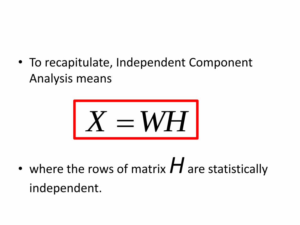
• To recapitulate, Independent Component Analysis means
• where the rows of matrix H are statistically
independent.
WHX
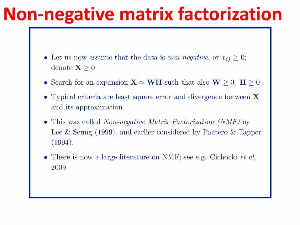
Non-negative matrix factorization
• NMF and its extensions is today quite an active research topic
– Tensor factorizations (Cichocki et al, 2009)
– Low-rank approximation (LRA) (Markovsky, 2012)
– Missing data (Koren et al, 2009)
– Robust and sparse PCA (Candés et al, 2011)
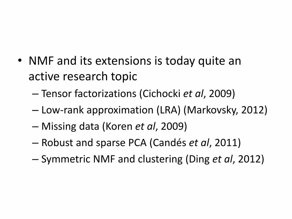
– Symmetric NMF and clustering (Ding et al, 2012)

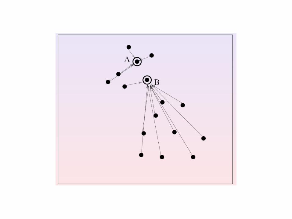
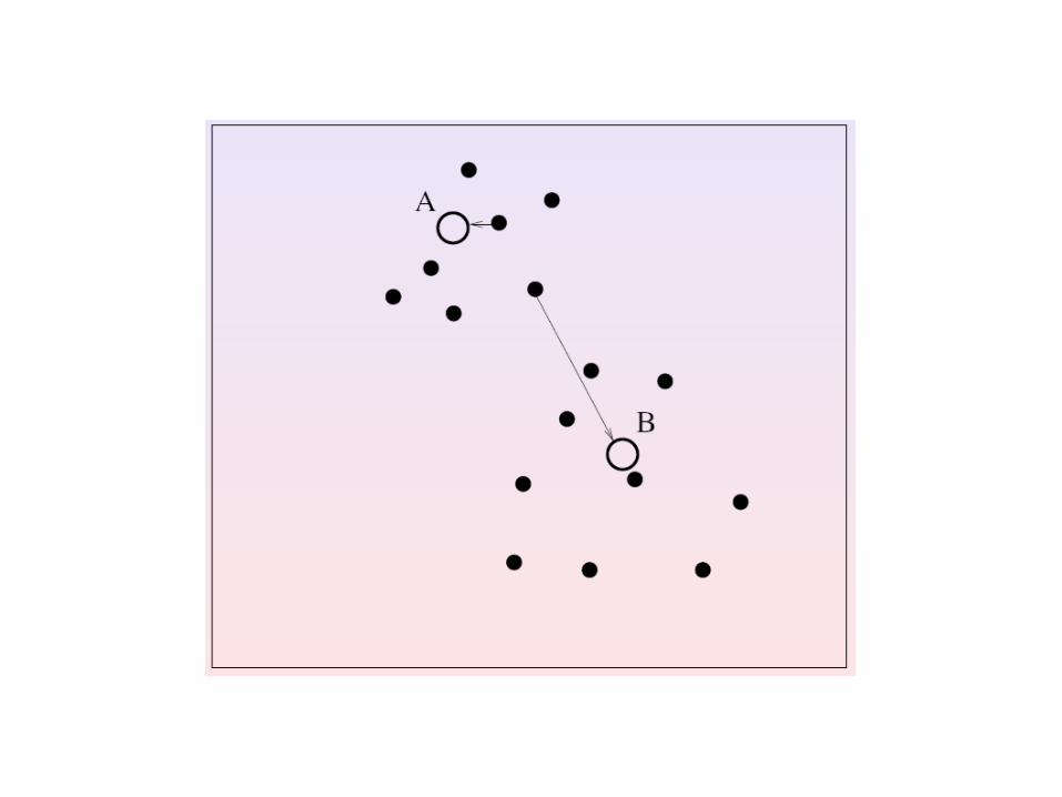
NMF and clustering
• Clustering is a very classical problem, in which n vectors (data items) must be partitioned into r clusters.
• The clustering result can be shown by the nxr cluster indicator matrix H
• It is a binary matrix whose element if and only if the i-th data vector belongs to the j-th cluster
1ijh
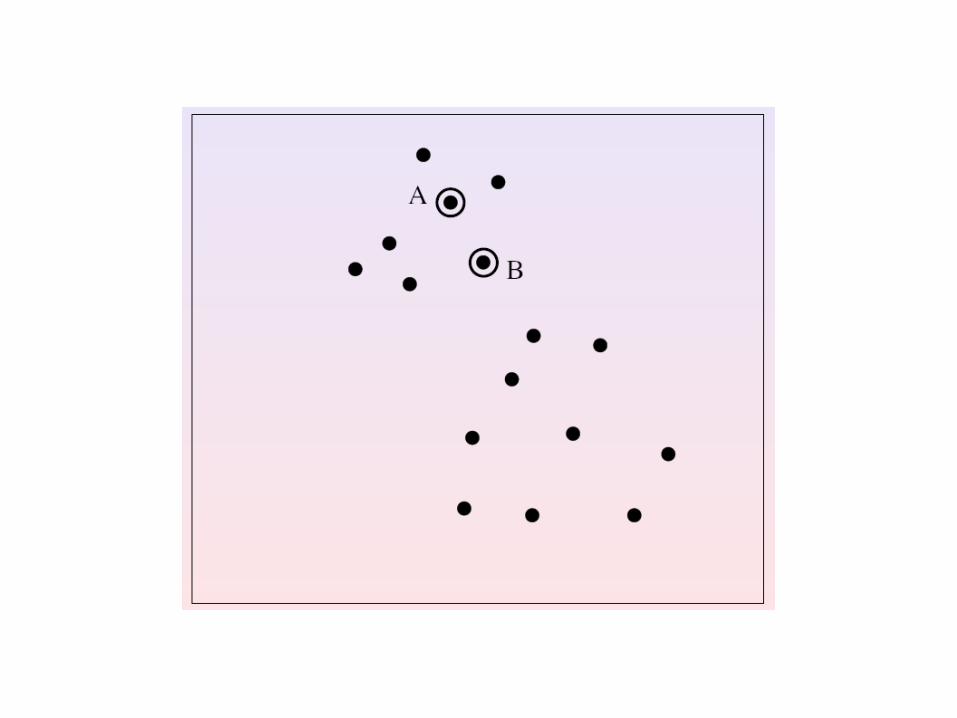
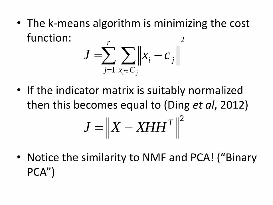
• The k-means algorithm is minimizing the cost function:
• If the indicator matrix is suitably normalized then this becomes equal to (Ding et al, 2012)
• Notice the similarity to NMF and PCA! (“Binary PCA”)
2
1
r
j Cx
ji
ji
cxJ
2TXHHXJ
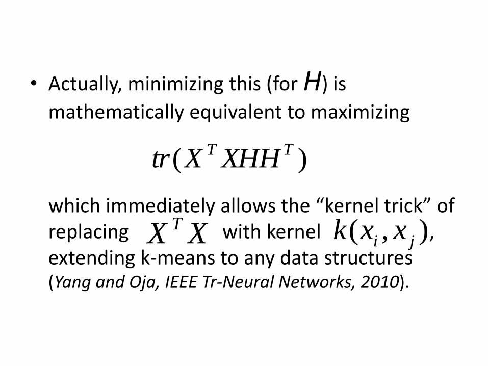
• Actually, minimizing this (for H) is
mathematically equivalent to maximizing
which immediately allows the “kernel trick” of replacing with kernel , extending k-means to any data structures (Yang and Oja, IEEE Tr-Neural Networks, 2010).
)( TT XHHXtr
XX T ),( ji xxk
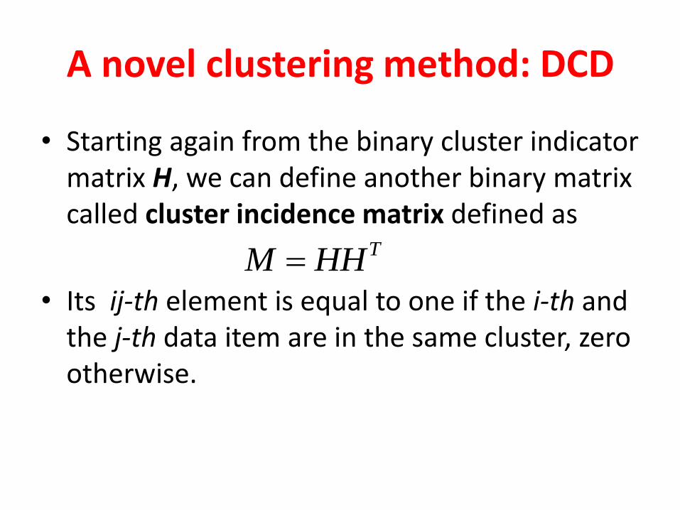
A novel clustering method: DCD
• Starting again from the binary cluster indicator matrix H, we can define another binary matrix called cluster incidence matrix defined as
• Its ij-th element is equal to one if the i-th and the j-th data item are in the same cluster, zero otherwise.
THHM
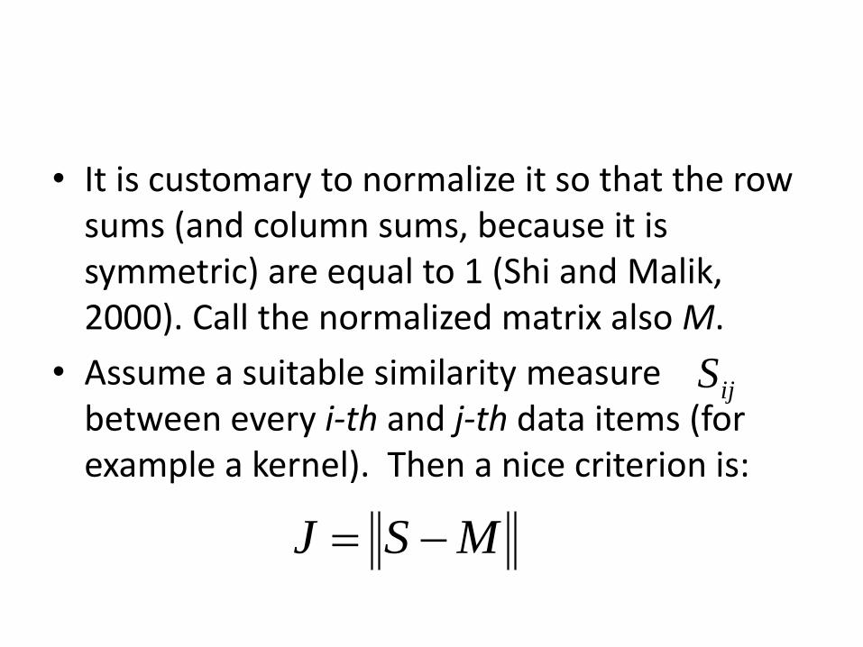
• It is customary to normalize it so that the row sums (and column sums, because it is symmetric) are equal to 1 (Shi and Malik, 2000). Call the normalized matrix also M.
• Assume a suitable similarity measure between every i-th and j-th data items (for example a kernel). Then a nice criterion is:
ijS
MSJ
• This is an example of symmetrical NMF because both the similarity matrix and the incidence matrix are symmetrical, and both are naturally nonnegative.
• S is full rank, but the rank of M is r.
• Contrary to the usual NMF, there are two extra constraints: the row sums of M are equal to 1, and M is a (scaled) binary matrix.
• The solution: probabilistic relaxation to smooth the constraints (Yang, Corander and Oja,
JMLR, 2016)
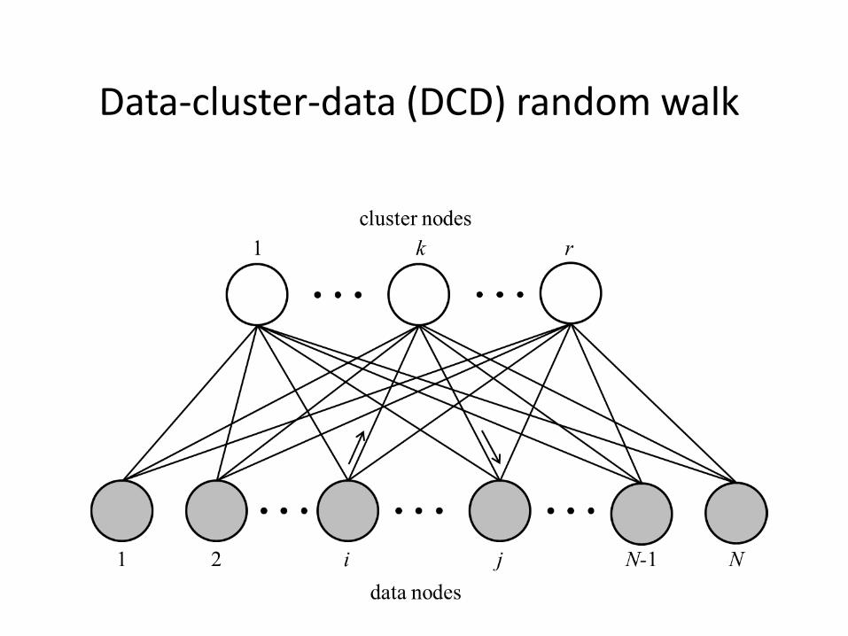
Data-cluster-data (DCD) random walk
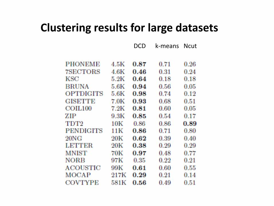
Clustering results for large datasets
DCD k-means Ncut
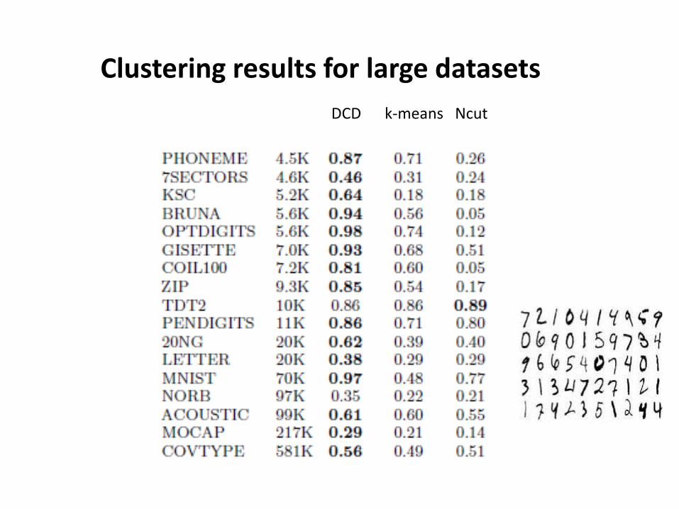
Clustering results for large datasets
DCD k-means Ncut

• To recapitulate, CDC clustering means
• Where S is the similarity matrix and
is a weighted binary matrix with both the row and column sums equal to one.
• Approximation by suitable divergence measure like Kullback-Leibler.
THHS
THH
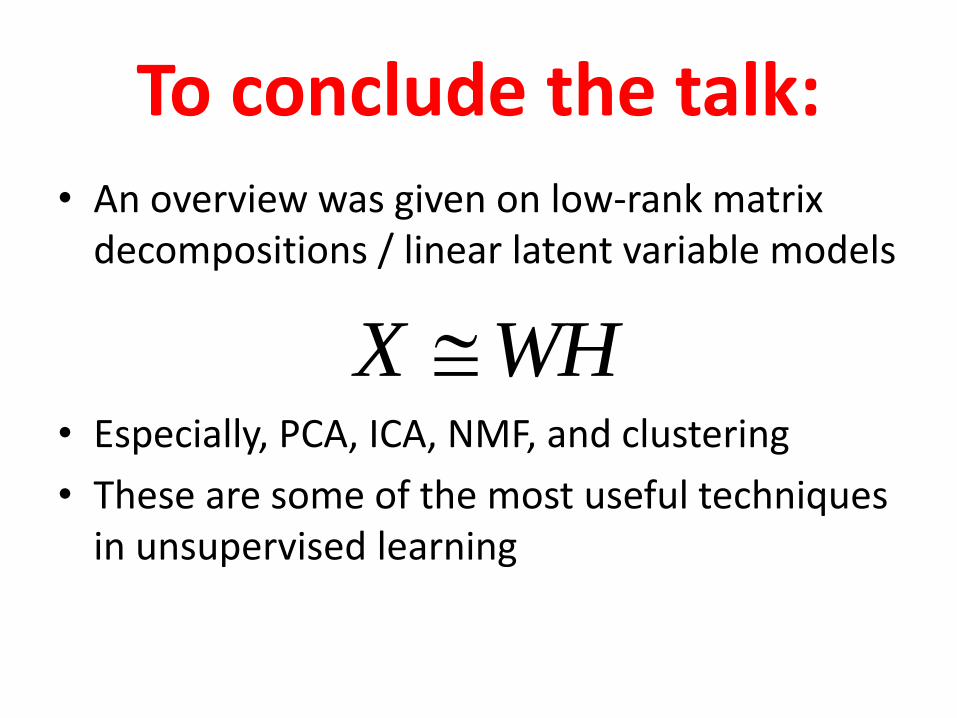
To conclude the talk: • An overview was given on low-rank matrix
decompositions / linear latent variable models
• Especially, PCA, ICA, NMF, and clustering
• These are some of the most useful techniques in unsupervised learning
WHX

• While such linear models seem deceivingly simple, they have some advantages:
– They are computationally simple
– Because of linearity, the results can be understood: the factors can be explained contrary to “black-box” nonlinear models such as neural networks
– With nonlinear cost functions and constraints, powerful criteria can be used.

THANK YOU FOR YOUR ATTENTION!

Additional material
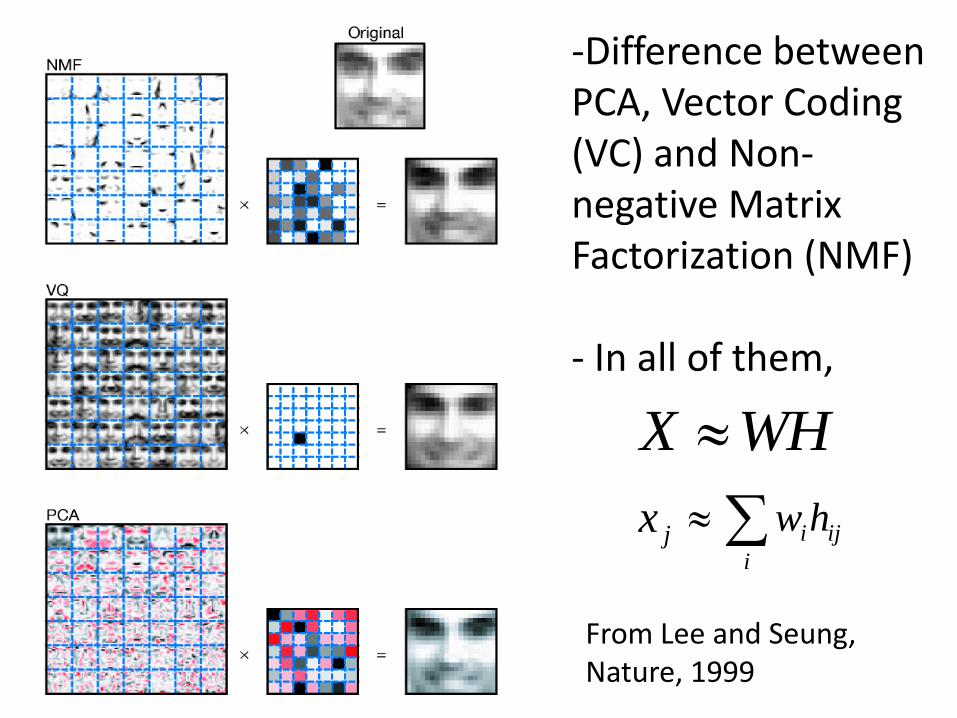
From Lee and Seung, Nature, 1999
-Difference between PCA, Vector Coding (VC) and Non-negative Matrix Factorization (NMF) - In all of them, WHX
jx ij
i
ihw


![Feature Learning with Matrix Factorization Applied to Acoustic … · 2016. 12. 4. · Victor Bisot, Romain Serizel, ... [21] by comparing popular unsupervised matrix factorization](https://img.pdfslide.us/doc/110x75/60d66ffc3229cb41555a25a3/feature-learning-with-matrix-factorization-applied-to-acoustic-2016-12-4-victor.jpg)