Embed Size (px)
Citation preview
An optimization model for buyer-supplierco-ordination under limited warehousespace and incremental price discount
Sahabuddin Sarwardi(†)∗
(†) Department of Mathematics, Aliah University, IIA/27, New TownKolkata - 700 156, West Bengal, India
email: [email protected]
Abstract
This paper considers incremental price discount, limited warehouse space and pay-ments delay. It is often seen that when a retailer purchases products for whichsupplier offers incremental price discounts. In Goyel [1] investigated the inventoryreplenishment problem under condition of payments delay, where he assumed that:(i) The unit selling price and unit purchasing price are equal (ii) The retailer startspaying higher interest charges on the items in stocks and returns money of theremaining balance immediately when the items are sold (iii) Retailer warehousespace is unlimited. Here we consider that unit purchasing price are not constantbut buyer has taken advantage of offering incremental price discount given by sup-plier. It is assumed that the buyer will borrow total purchasing cost from the bankto pay off the account, buyer must pay the amount of purchasing cost to the sup-plier at the end of trade credit period. This also assumed that the buyer’s storagespace is limited. Numerical examples are given to illustrate results obtained in ofthe present study.
Keywords: Inventory, Production, Optimization, Price setting, Quantity discount, Lim-ited Warehouse space, Payments delay.
1 Introduction
Offering quantity discounts is a common industrial practice. Some of the reasons so faroffering quantity discounts are as follows:
∗Author to whom all correspondence should be addressed
(1) to stimulate the demand for the product;
(2) to reduce per-unit set-up cost for the supplier;
(3) to meet competition.
Although all unit discount schedule are more common, many suppliers offer incrementaldiscounts. In an incremental discount schedule, lower unit-price is applicable only to theincremental quantity.
In the classical incremental discount economic order quantity model, demand for theproduct is considered to be constant (cf. Hadley and Whitin [2], Max and Candea [3],Tersine and Toelle [4], Jackson and Munson [5], Tamjidzad and MirMuhammai [6]). Arelated paper considers all-unit type quantity discounts schedule (cf. Abad [7]-[8]). InKunreuther and Richard [9], the pricing and lot-sizing problem for the linear demandand no quantity discounts is considered. Tajbakhsh [10] also considered an inventorymodel with random discount. Down the years, a number of reseachers have appearedin the literature that treat inventory problem with varying conditions under paymentsdelay indeed to link financing marketing as well as operations concerned. Some of theprominent papers are discussed here. Goyel [1] established a single item inventory modelunder trade credit. Chen and Chuang [11] investigated light buyer’s inventory policyunder trade credit by the concept of discounted cash flow. Sarkar et al. [12] investigatedthis topic with inflation. Jamal et al. [13] addressed the optimal payment time underpermissible delay in payments and deterioration. Chung and Huang [14] developed anefficient procedure to determine the retailer’s optimal ordering policy. Supplier usesfavorable trade credit policy to encourage retailer to order large quantities because adelay in payments indirectly reduces inventory cost (cf. Ting [15]). Hence, the retailermay purchase more goods than that can be stored in his/her own warehouse. Theseexcess quantities are stored in a rented warehouse. This proposed model is applicablefor the business of small and medium sized firm since their storage capacity are smalland limited. In general, the inventory holding charges in rented warehouse is greaterthan that for own warehouse. When the demand occurs, it first is replenished from therented warehouse. This is done to reduce inventory holding costs. It is assumed thatthe transportation costs between warehouses are negligible. This viewpoint can be foundin Sarma [16], Pakkala and Achary[17], Goswami and Chaudhuri [18], Benkherouf [19],Bhunia and Maiti [20], and Onal [21].
2 Model formulation
The integrated production inventory model proposed in this paper is based on the fol-lowing notations and assumptions:
(1) n raw materials are required to manufacture a single final product.
2
(2) The production rate of the final item is P (constant).
(3) The demand rate of the final item is price sensitive and is given by
D(p) = Kp−e, e > 1, K > 0,
where p is the selling price of unit final item together with P > D(p).
(4) The raw materials are received from out-supplier at an infinite rate of replenishment.
(5) The supplier of raw materials offers an incremental price discount to the manufacturer.Manufacturer’s purchase per unit item is of the following pattern (cf. Abad [8], Naddor[22]):
v(q) =
v1, for q0 ≤ q < q1,v2, for q1 ≤ q < q2,v3, for q2 ≤ q < q3,. . . . . . . . . . . . . . . . . . . . . . . .. . . . . . . . . . . . . . . . . . . . . . . .vn−1, for qn−2 ≤ q < qn−1,vn, for q ≥ qn,
where q is the quantity of raw materials to be purchased and vn is a strictly monotonicdecreasing sequence.
(6) Supplier of raw materials also offers a trade off credit period M . If the credit periodis shorter than the cycle length, the manufacturer sale them and accumulate sales revenueand earned interest throughout the cycle.
(7) Shortages of raw materials and final product are not allowed.
(8) T is the inventory cycle time and T1 is the production run of the final product.
(9) Let I(t) is the inventory level of the final product and Ir(t) is the inventory level ofthe raw materials at time t.
(10) Let Qr is the amount of raw materials to be purchased by the manufacturer and itscorresponding cost is V (Qr)
(11) Manufacturer must pay the amount of the purchasing raw materials to the supplierat time M .
(12) Manufacturer has finite storage capacity W . If the ordered quantity is larger thanthe manufacturer’s storage space then he will rent a warehouse to store the exceedingitems. It is to be noted that, when manufacturing starts it start production by using rawmaterials from the rented warehouse.
3
2.1 Some notations:
Am = cost of placing an order.
Dr = demand of raw materials, Dr = nP.
p = unit selling price of the final item.
Cm = production cost of unit final item excluding the raw material cost.
hr = unit raw material holding cost of own warehouse per year.
kr = unit raw material holding cost of rented warehouse per year.
h = unit finished good holding cost.
Ch = total finished good holding cost.
Ie = annual interest earned rate.
Ip(> Ie) = annual interest charged rate.
M = trade credit period (constant).
T1 = supplying duration of raw materials.
Qr = lot size of raw materials.
Q = lot size of final items.
T = the cycle length.
W = manufacturer’s own storage capacity.
tW = the rented house time given by the following equations:
tW =
{DrT1−W
Dr, if T1 >
WDr
0, if T1 ≤ WDr
.
B = capital amount invested by the manufacturer.
2.2 The model and optimality condition
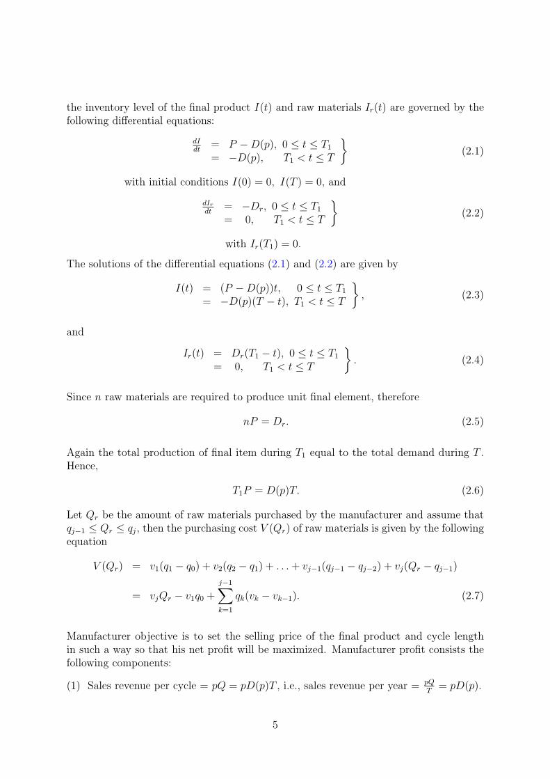
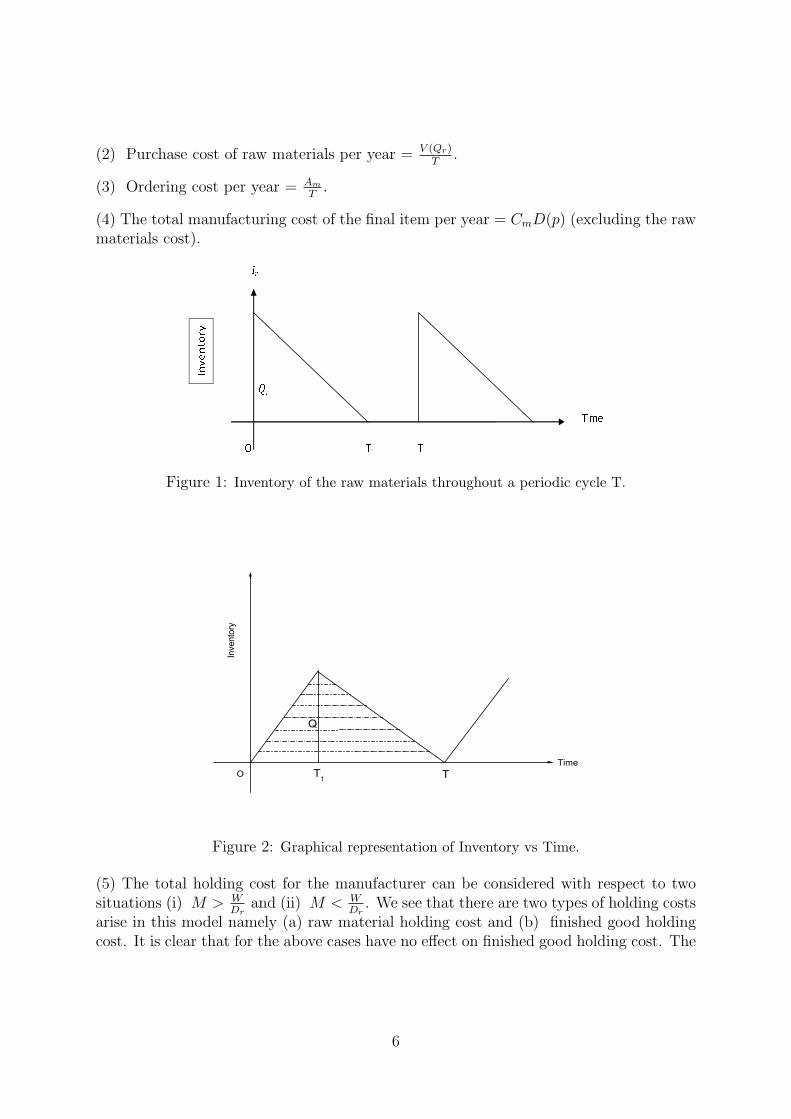
Insert Figures 1 and 2 here
Let us consider that the consumption rate of raw materials is Dr and the consumptioncontinue up to T1(< T ). At the beginning of each cycle, the required raw material arereceived and the production stage of the final item starts. In this stage the variation of
4
the inventory level of the final product I(t) and raw materials Ir(t) are governed by thefollowing differential equations:
dIdt
= P −D(p), 0 ≤ t ≤ T1
= −D(p), T1 < t ≤ T
}(2.1)
with initial conditions I(0) = 0, I(T ) = 0, and
dIrdt
= −Dr, 0 ≤ t ≤ T1
= 0, T1 < t ≤ T
}(2.2)
with Ir(T1) = 0.
The solutions of the differential equations (2.1) and (2.2) are given by
I(t) = (P −D(p))t, 0 ≤ t ≤ T1
= −D(p)(T − t), T1 < t ≤ T
}, (2.3)
and
Ir(t) = Dr(T1 − t), 0 ≤ t ≤ T1
= 0, T1 < t ≤ T
}. (2.4)
Since n raw materials are required to produce unit final element, therefore
nP = Dr. (2.5)
Again the total production of final item during T1 equal to the total demand during T .Hence,
T1P = D(p)T. (2.6)
Let Qr be the amount of raw materials purchased by the manufacturer and assume thatqj−1 ≤ Qr ≤ qj, then the purchasing cost V (Qr) of raw materials is given by the followingequation
V (Qr) = v1(q1 − q0) + v2(q2 − q1) + . . .+ vj−1(qj−1 − qj−2) + vj(Qr − qj−1)
= vjQr − v1q0 +
j−1∑k=1
qk(vk − vk−1). (2.7)
Manufacturer objective is to set the selling price of the final product and cycle lengthin such a way so that his net profit will be maximized. Manufacturer profit consists thefollowing components:
(1) Sales revenue per cycle = pQ = pD(p)T , i.e., sales revenue per year = pQT
= pD(p).
5
(2) Purchase cost of raw materials per year = V (Qr)T
.
(3) Ordering cost per year = Am
T.
(4) The total manufacturing cost of the final item per year = CmD(p) (excluding the rawmaterials cost).
Figure 1: Inventory of the raw materials throughout a periodic cycle T.
Q
TT1
Time
Inve
ntory
O
Figure 2: Graphical representation of Inventory vs Time.
(5) The total holding cost for the manufacturer can be considered with respect to twosituations (i) M > W
Drand (ii) M < W
Dr. We see that there are two types of holding costs
arise in this model namely (a) raw material holding cost and (b) finished good holdingcost. It is clear that for the above cases have no effect on finished good holding cost. The
6
I
Q
Time
O T� T M
Inv
en
tory
P > D(p)
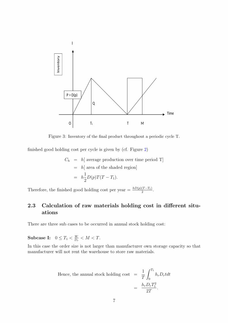
Figure 3: Inventory of the final product throughout a periodic cycle T.
finished good holding cost per cycle is given by (cf. Figure 2)
Ch = h[ average production over time period T]
= h[ area of the shaded region]
= h1
2D(p)T (T − T1).
Therefore, the finished good holding cost per year = hD(p)(T−T1)2
.
2.3 Calculation of raw materials holding cost in different situ-ations
There are three sub cases to be occurred in annual stock holding cost:
Subcase I: 0 ≤ T1 <WDr
< M < T .
In this case the order size is not larger than manufacturer own storage capacity so thatmanufacturer will not rent the warehouse to store raw materials.
Hence, the annual stock holding cost =1
T
∫ T1
0
hrDrtdt
=hrDrT
21
2T.
7
MTM
Q
T1
Time
Inventory
O
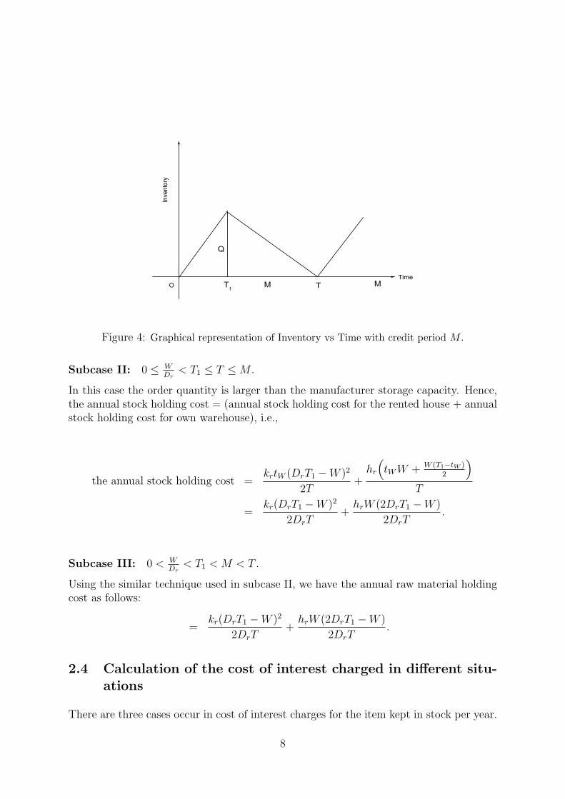
Figure 4: Graphical representation of Inventory vs Time with credit period M .
Subcase II: 0 ≤ WDr
< T1 ≤ T ≤ M .
In this case the order quantity is larger than the manufacturer storage capacity. Hence,the annual stock holding cost = (annual stock holding cost for the rented house + annualstock holding cost for own warehouse), i.e.,
the annual stock holding cost =krtW (DrT1 −W )2
2T+
hr
(tWW + W (T1−tW )
2
)T
=kr(DrT1 −W )2
2DrT+
hrW (2DrT1 −W )
2DrT.
Subcase III: 0 < WDr
< T1 < M < T .
Using the similar technique used in subcase II, we have the annual raw material holdingcost as follows:
=kr(DrT1 −W )2
2DrT+
hrW (2DrT1 −W )
2DrT.
2.4 Calculation of the cost of interest charged in different situ-ations
There are three cases occur in cost of interest charges for the item kept in stock per year.
8
Case I: 0 ≤ T1 < M < T .
In this case the credit period is larger than the cycle length. Hence no interest is chargedfor the item kept in the stock.
Case II: T1 < T < M .
Similar as in case I, no interest is charged for the item kept in the stock.
Case III: T > M .
In this case cost of interest charged for the items kept in the stock per year is
=IpV (Qr)(T −M)
T.
2.5 Calculation of the cost of interest earned per year in differ-ent situations
There are three cases occur in interest earned per year.
Case I: 0 ≤ T1 ≤ WDr
< M < T .
In this case the manufacturer sell the items and earned interest until the end of the creditperiod. Hence in this case the total interest earned per year is
= pIe
[12D(p)T 2 +D(p)T (M − T )
]T
= D(p)Iep
(M − T
2
).
Case II: 0 < WDr
< T1 < T < M .
Similar as in case I, total interest earned per year is
= D(p)Iep
(M − T
2
).
Case III: T > M .
In this case the manufacturer can sell the items and earned interest throughout the
9
inventory cycle. Hence the total interest earned per year is
= pIe1
T
∫ T
0
D(p)tdt
=IepD(p)T
2.
From the above argument the total annual profit for the manufacturer can expressed as
maxΠ(p, T, T1) = sales revenue - manufacturing cost - ordering cost - inventory
holding cost - interest charged cost + interest earned cost.
Thus, the total annual profit Π(p, T, T1) takes the following form:
Π(p, T, T1) =
Π1(p, T, T1), if 0 ≤ T1 < T ≤ W
Dr< M,
Π2(p, T, T1), if 0 < WDr
< T1 ≤ T ≤ M,
Π3(p, T, T1), if T > M,
(2.1)
where
Π1(p, T, T1) = (p− Cm)D(p)− V (Qr)
T− Am
T− hD(p)(T − T1)
2− hrDrT
21
2T
+IeD(p)
(M − T
2
), (2.2)
Π2(p, T, T1) = (p− Cm)D(p)− Am
T− hD(p)(T − T1)
2+ IeD(p)
(M − T
2
)−V (Qr)
T−(kr(DrT1 −W )2
2DrT+
hrW (2DrT1 −W )
2DrT
), (2.3)
and
Π3(p, T, T1) = (p− Cm)D(p)− V (Qr)
T− Am
T− IpV (Qr)(T −M)
T+
pIeD(p)T
2
− hD(p)(T − T1)
2−
(kr(DrT1 −W )2
2DrT+
hrW (2DrT1 −W )
2DrT
). (2.4)
If n raw materials are required to produce the final item. Therefore, Qr = nQ = nD(p)T ,
10
also we have
V (Qr)
T=
vjQr − V0
T, where V0 = v1q0 −
∑j−1k=1 qk(vk − vk−1)
= nvjD(p)− V0
T. (2.5)
Substituting the value of T1 from (2.6) and using the equation (2.5), manufacturer’sannual profit function defined in (2.1) is reduced to the following one:
Π(p, T ) =
Π1(p, T ), if 0 ≤ T1 < T ≤ W
Dr< M,
Π2(p, T ), if 0 < WDr
< T1 ≤ T ≤ M,
Π3(p, T ), if T > M,
(2.6)
where
Π1(p, T ) = (p− Cm − nvj)D(p)− Am − V0
T− hD(p)T
2
(1− D(p)
P
)− hrDrD
2(p)T
2P 2
+IeD(p)
(M − T
2
), (2.7)
Π2(p, T ) = (p− Cm − nvj)D(p)− Am − V0
T− hD(p)T
2
(1− D(p)
P
)+ IeD(p)
(M − T
2
)
−
[kr(nD(p)T −W
)2
2DrT+
hrW
(2nD(p)T −W
)2DrT
], (2.8)
and
Π3(p, T ) = (p− Cm − nvj)D(p)− Am − V0
T− hD(p)T
2
(1− D(p)
P
)
−
[kr(nD(p)T −W
)2
2DrT+
hrW
(2nD(p)T −W
)2DrT
]
+IepD(p)T
2− Ip
(nvjD(p)− V0
T
)(T −M). (2.9)
11
Thus, our problem is to maximize the objective function
Π(p, T ) =
Π1(p, T ), if 0 ≤ T1 < T ≤ W
Dr< M,
Π2(p, T ), if 0 < WDr
< T1 ≤ T ≤ M,
Π3(p, T ), if T > M,
(2.10)
subject to the following conditions:
(i) P > D(p),
(ii) B ≥ V (Qr) + CmQ,
(iii) p >nV (Qr)
Qr
+ Cm.
As it is tough to undertake the above constrained maximization problem analytically, wemust directed to solve this problem numerically.
3 Numerical simulation
In this section we consider two types of demand rates of final item Case (i): constantprice elasticity demand function: D(p) = Kp−e , where K(> 0) is the scaling factor ande is (constant) price elasticity. This demand function is applicable for those commoditieswhose price elasticity e > 1. Case (ii): the linear demand function: D(p) = a − bp,where a, b are positive constants and p < a
b. For the first case, if we choose the following
hypothetical values of the parameters P = 5000; Cm = 1; n = 5; h = 1; hr = 0.25;kr = 0.5; K = 2; e = 1.5; M = 0.2; Dr = 35000; Ie = 0.05; Ip = 0.09; W = 2000;Am = 500; j = 4; T = 0.6; q0 = 0; q1 = 100; q2 = 500; q3 = 1000; q4 = 1500; v1 = 10;v2 = 9.5; v3 = 9.0; v4 = 8.5; v5 = 7.0 then we have the optimal value of selling pricep → 122.145 and corresponding maximum profit is found from max(Π1(p, T )) → 2166.66.It is to be noted that these optimal decision values also satisfy all the constraints for thisobjective function.
If we consider the linear trend demand function D(p) = a − bp, for the following set ofvalues of the parameters: P = 5000; Cm = 0.2; n = 5; h = 0.5; hr = 0.8; kr = 0.5;M = 0.5; Dr = 25000; Ie = 0.05; Ip = 0.08; W = 8000; Am = 500; j = 4; q0 = 0;q1 = 130; q2 = 500; q3 = 1000; q4 = 1500; v1 = 10; v2 = 9.5; v3 = 9.0; v4 = 8.5; v5 = 7.0;T = 0.4 < M = 0.5; a = 4000; b = 15, then we have the optimal value of selling pricep → 155.1 and corresponding maximum profit is obtained by max(Π2(p, T )) → 184604.
These parameter values satisfy the restrictions given in Case (ii). To find the numericalsolution I have taken the help of the built-in function ‘FindMaximum’ in Mathematicasoftware [23].
12
4 Concluding remarks
We have considered in this paper the joint price and cycle length determination problemfaced by retailer when he purchase products for which the supplier offers incrementalquantity discounts. Incremental discounts are offered in practice in many realistic situ-ation. It is reported that the Figures: 1–4 are given for different inventory levels withrespect to time. Our observations have shown that linear trend demand is more profitablethan that of constant price elasticity demand.
Acknowledgement: The author Dr. S. Sarwardi is thankful to the Department ofMathematics, Aliah University for providing opportunities to perform research work. Heis also thankful to Dr. B. C. Giri, Department of Mathematics, Jadavpur University,Kolkata for providing his generous help, suggestions and interpretations of results ob-tained.
References
[1] Goyel, S.K. 1985. Economic order quantity under conditions of permissible delay in pay-ments. Journal of Operational Research Society.36, 335-338.
[2] Hadley, G. & Whitin, T.M. 1964. Analysis of Inventory System. Prentice Hall. EnglewoodCliffs, New Jersey.
[3] Max, A.C. & Candea, D. 1984. Production and Inventory Management. Prentice Hall.Englewood Cliffs, New Jersey.
[4] Tersine, R.J. & Toelle, R.A. 1985. Lot-size determination with quantity discounts. Prod.Invent. Mgmt. 26, 1-23.
[5] Jackson, J.E. Munson, C.L. 2016. Shared resource capacity expansion decisions for multi-ple products with quantity discounts. European Journal of Operational Research. 253,602-613.
[6] Tamjidzad, S. & Mirmohammadi, S. 2017. Optimal (r, Q) policy in a stochastic inven-tory system with limited resource under incremental quantity discount. Computers &Industrial Engineering. 103, 59-69.
[7] Abad, P.L. 1986. Determining optimal price and lot-size when supplier offers all-unitquantity discounts. Technical Paper, Faculty of Business. McMaster University. Hamil-ton. Canada.
[8] Abad, P.L. 1986. Joint price and lot-size determination when supplier offers incremen-tal quantity discounts. Technical Paper, Faculty of Business. McMaster University.Hamilton. Canada.
[9] Kunreuther, H. & Richard, J.F. 1971. Optimal pricing and inventory decisions for non-seasonal items. Econometrica. 39, 173-175.
13
[10] Tajbakhsh, M.M., Lee, C.G. & Zolfaghari, S. 2011. An inventory model with randomdiscount offerings. Omega 39, 710-718.
[11] Chen, M.S. & Chuang, C.C. 1999. An analysis of light buyer’s economic order modelunder trade credit. Asia-Pacific Journal of Operational Research. 16, 23-34.
[12] Sarkar, B.R., Jamal, A.M.M. & Wang, S. 2000. Supply chain model of perishable prod-ucts under inflation and permissible delay in payment. Computers and OperationsResearch Society. 27, 59-75.
[13] Jamal, A.M.M., Sarkar, B.R. & Wang, S. 2000. Optimal payment time for a retailer un-der permitted delay of payment by the wholesaler. International Journal of ProductionEconomics. 66, 157-167.
[14] Chung, K.J. & Huang, Y.F. 2003. The optimal cycle time for EPQ inventory modelunder permissible delay in payments. International Journal of Production Economics.84, 307-318.
[15] Ting, P.S. 2015. Comments on the EOQ model for deteriorating items with conditionaltrade credit linked to order quantity in the supply chain management. European Journalof Operational Research. 00, 1-11.
[16] Sarma, K.V.S. 1980. A deterministic order level inventory model for deteriorating itemswith two storage facilities. European Journal of Operational Research. 29, 70-73.
[17] Pakkala, T.P.M. & Achary, K.K. 1992. A deterministic inventory model for deterio-rating items with two warehouses and finite replenishment rate. European Journal ofOperational Research. 57, 71-76.
[18] Goswami, A. & Chaudhuri, K.S. 1992. An economic order quantity model for items withtwo levels of storage for a linear trend in demand. Journal of the Operational ResearchSociety. 43, 157-167.
[19] Benkherouf, L. 1997. A deterministic order level inventory model for deteriorating itemswith two storage facilities. International Journal of Production Economics. 48, 167-175.
[20] Bhunia, A. K. & Maiti, M. 1998. A two-warehouse inventory model for deterioratingitems with a linear trend in demand and shortages. Journal of the Operational ResearchSociety.49, 287-292.
[21] Onal, M. 2016. The Two-Level Economic Lot Sizing Problem with Perishable Items.Operations Research Letters. 44, 403-408.
[22] Naddor, E. 1966. Inventory systems. John Willey & Sons, Inc. New York.
[23] Wolfram, S. 2003. The Mathematica Book. Fifth Edition. Wolfram Media. CambridgeUniversity Press.
14