GEOPHYSICS, VOL. 60, NO.1 (JANUARY-FEBRUARY 1995); P. 296-301, 4 FIGS.

Short Note

An optimal absorbing boundary condition forelastic wave modeling

Chengbin Peng* and M. Nafi Toksozt

INTRODUCTION

+ alOvn(k, j, 0) + al1vn(k, j, 1)

+ a12vn(k, j, 2) + a20Vn-1(k, j, 0)

+ a21Vn- 1(k,j, 1) +a22Vn-1(k,j, 2),

(4)

(2)

(3)

(5)

2~" 0 0 + 0IZa + 02Z;

Rps

= - ~ + " 0 0 + 01Zb1 + 02Zb2'

2 0 0 + 0IZb + 02Z~R sp = -/:-- -1 -2 '

.. + " 0 0 + 0IZa + 02Za

~ -" 0 0 + 0IZb + 02Z~R ss = -- -1 -2 '

~ + " 0 0 + 01Zb + 02Zb

(1)

where the coefficients {aij}(aOO == 0) are chosen such thatreflection from the artificial boundary x = 0 is as small aspossible. In an acoustic case, equation (1) is applied directlyto a pressure field on the artificial boundary. When elasticenergy is to be absorbed, equation (1) is applied to eachcomponent of the elastic wave. In this scheme, only gridsperpendicular to the boundary are used in the extrapolationprocess. Attention is also restricted to the case where theextrapolation operator is two steps in both time and space;i.e., a (2, 2) scheme, where the first and second numbersrefer to the steps in time and space, respectively.

The reflection coefficients from the boundary x = 0 are(Peng and Toksoz, 1994):

~ -" 0 0 + 0IZa + 02Z;

Rpp = Z--+ rl rl -1 rl -2'.. "uo + ulZa + U2Za

STRUCTURES OF REFLECTION COEFFICIENTS

Absorbing boundary conditions are widely used in numer­ical modeling of wave propagation in unbounded media toreduce reflections from artificial boundaries (Lindman, 1975;Clayton and Engquist, 1977; Reynolds, 1978; Liao et aI.,1984; Cerjan et aI., 1985; Randall, 1988; Higdon, 1991). Weare interested in a particular absorbing boundary conditionthat has maximum absorbing ability with a minimum amountof computation and storage. This is practical for 3-D simu­lation of elastic wave propagation by a finite-differencemethod. Peng and Toksoz (1994) developed a method todesign a class of optimal absorbing boundary conditions fora given operator length. In this short note, we give a briefintroduction to this technique, and we compare the optimalabsorbing boundary conditions against those by Reynolds(1978) and Higdon (1991) using examples of 3-D elasticfinite-difference modeling on an nCUBE-2 parallel com­puter. In the Appendix, we also give explicit formulas forcomputing coefficients of the optimal absorbing boundaryconditions.

Let vn(k,j, i) denote a wavefield at (z = ktJ.z,y = jt:.y,x = it:.x) and at time t = n St . In the interior of afinite-difference grid, v is updated according to the differenceapproximations of wave equations. On the artificial bound­aries, extrapolation based on values at previous time stepsand interior grids is needed to minimize unwanted reflec­tions.

We can write v n +1(k , j , 0) on the artificial boundary, e.g.,x = 0, as a linear combination of fields at previous time stepsand atx ~ 0 as:

Manuscript received by the Editor February 22, 1993; revised manuscript received June 29, 1994.·Form~rly Earth Resources Laborato~, Department of Earth, Atmospheric, and Planetary Sciences, Massachusetts Institute of Technology,Cambndge, MA 02139; presently Bellaire Research Center, Shell Development Company, P.O. Box 481, Houston, TX 77001-0481.:j:Earth Resources Laboratory, Department of Earth, Atmospheric, and Planetary Sciences, Massachusetts Institute of TechnologyCambridge, MA 02139. '© 1995 Society of Exploration Geophysicists. All rights reserved.

296

Dow

nloa

ded

05/1

2/13

to 1

29.1

00.2

49.5

0. R

edis

trib

utio

n su

bjec

t to

SEG

lice

nse

or c

opyr

ight

; see

Ter

ms

of U

se a

t http

://lib

rary

.seg

.org

/

Optimal Absorbing Boundary Condition 297

where R pp and R ps are the P-wave to P-wave and P -wave toS-wave reflection coefficients, and R sp and R ss are theS-wave to P-wave and S-wave to S-wave reflection coeffi­cients, respectively, and where and

L (aiO - ai2) = 1,i=O

(13)

0 0 = aOOz + alO + a20z-1 -z,

0 1 = aOlz + all + a21z-l,

02 = a02z + a12 + a22z- 1,

(6)

(7)

(8)

where z = e i!Si,

and

" 2 .,£J a ij = rmmmum,i=O,j=O

(14)

-fr:!: = &X cos a:!:. (15)A fast algorithm given in the Appendix can be used todetermine the coefficient {aij}.

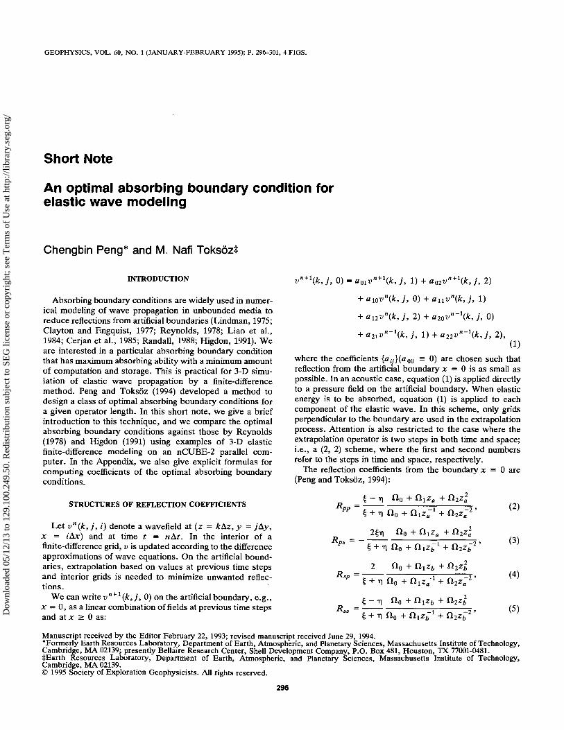
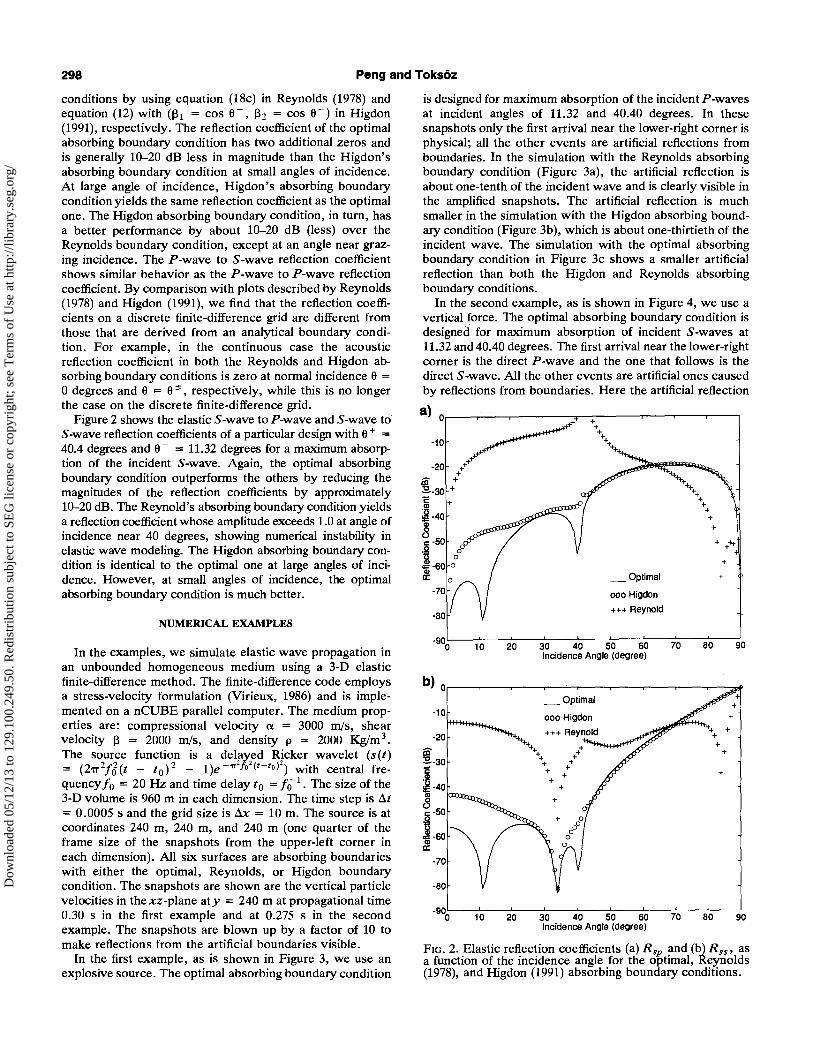
For a practical problem with a = 3000 mis, 13 = 2000 mis,At = 0.0005 s, /ix = 10 m, eo = 2'1T X 20 Hz, Figure 1 showsthe elastic P-wave to P-wave and P-wave to S-wave reflec­tion coefficients of a particular design with a + = 40.4degrees and a- = 11.32 degrees for a maximum absorptionof the incident P-wave. For comparison, we show also thereflection coefficients of the Reynolds and Higdon absorbing

a) O'.-----r---.-----,---...--r---,-----,----,--~

are the z-transforrns along columns of the coefficient matrix{aij}. In the above equations, z = eiwt:.t is a one-step shift intime, Za = elkacos 6.ix is a one-step shift in space with anapparent compressional velocity, Zb = eik~cos cj>.ix is aone-step shift in space with an apparent shear velocity, ~ =

f3/a cos a/sin <\>, and 1] = 13/a sin a/cos <\>, where a and 13 arethe compressional and shear velocities, respectively, eo is thefrequency, and k a = wla and kr. = w/f3 are the compres­sional and shear wavenumbers. a and <\> are the incidenceangles of the P-wave and S-wave waves, respectively, andare related by Snell's law: sin ala = sin <\>/13.

The reflection coefficients on a finite-difference grid havethe following structures; (1) the numerator is a space z-trans­form associated with the incident wave; (2) the denominatoris another space z-transform associated with the reflectedwave; (3) the coefficients 00' 01> and 02 are z-transformswith respect to time; (4) the numerator represents a wavepropagating toward the artificial boundary and is a polyno­mial of the positive power of z; and (5) the denominatorrepresents a wave reflected backward into the finite-differ­ence domain and is a polynomial of the negative power of z .It is interesting to point out that the reflection coefficients in(2)-(5), e.g., R pp , can be regarded as the combined transferfunctions of two cascaded subsystems: the first is the inverseof a causal feed-backward system with delay, and the secondis an anticausal feed-forward system with advance.

-10

-70

-80

_Optimal

000 Higdon

+++ Reynold

++

+

90

90

++

80

80

70

70

30 40 50 60Incidence Angle (degree)

20

20

_Optimal

000 Higdon

+++ Reynold

10

10

-20

-10

30 40 50 60Incidence Angle (degree)

FIG. 1. Elastic reflection coefficients, (a) R pp ~nd (b) RpS' asa function of the incidence angle for the optimal, Reynolds(1978), and Higdon (1991) absorbing boundary conditions.The vertical axis is the magnitude in dB of the reflectioncoefficients.

(12)

(10)

(11)" a··=1£J IJ 'i=O,j=O

L (aOj - a2j) = 1,j=O

OPTIMAL ABSORBING BOUNDARY CONDITIONS

a01z+all +a21z-1

-----------:-1 = -(cos -fr + + cos -fr _ )a02z + a12 + a22z

The inputs to our algorithm are two physical incidenceangles a + and a - at which either R pp or R ss is zero. Inaddition, the following quantities are needed: dimensionlesstime step At = wAt and grid size &X: = wla/ix for amaximum P-wave absorption or Ax = w/f3/ix for a maxi­mum S-wave absorption. The coefficients in equation (1) aredetermined by the following set of equations (Peng andToksoz, 1994):

a OoZ + a 10 + a 20z -1 - Z---------':"""1- = cos (-fr + + -fr -)

a 02z + a 12 + a 22z

Dow

nloa

ded

05/1

2/13

to 1

29.1

00.2

49.5

0. R

edis

trib

utio

n su

bjec

t to

SEG

lice

nse

or c

opyr

ight

; see

Ter

ms

of U

se a

t http

://lib

rary

.seg

.org

/

298 Peng and Toksoz

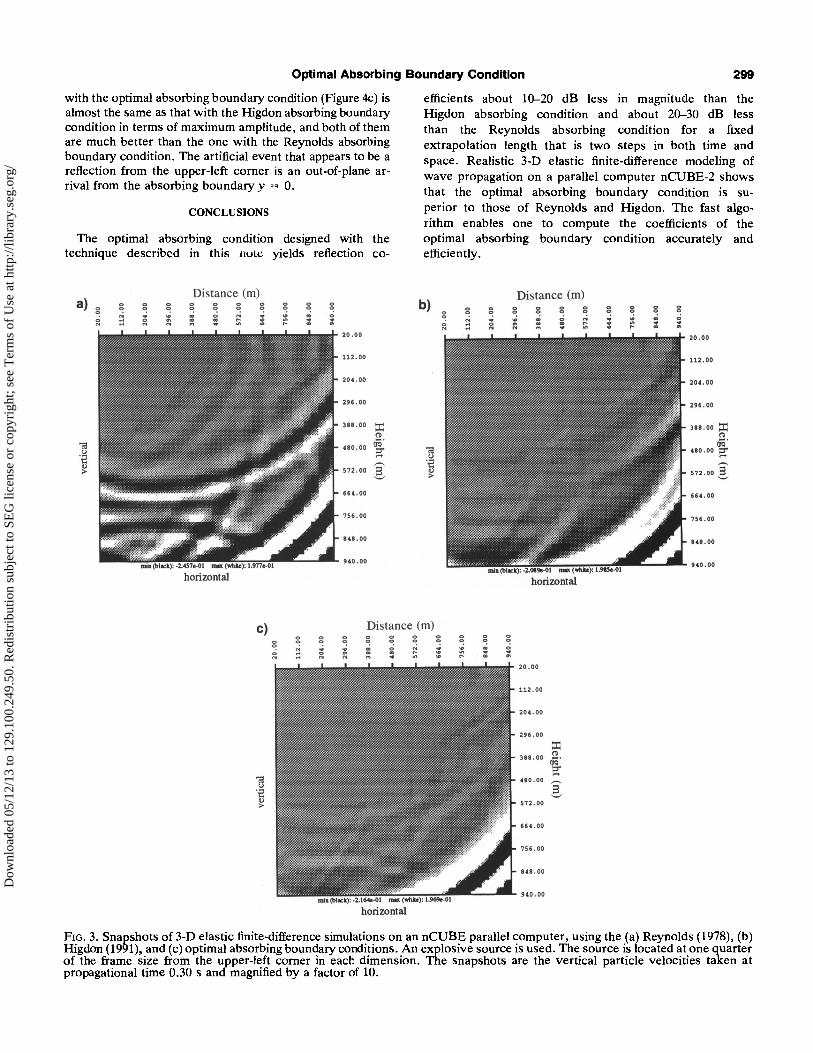
is designed for maximum absorption of the incident P-wavesat incident angles of 11.32 and 40.40 degrees. In thesesnapshots only the first arrival near the lower-right corner isphysical; all the other events are artificial reflections fromboundaries. In the simulation with the Reynolds absorbingboundary condition (Figure 3a), the artificial reflection isabout one-tenth of the incident wave and is clearly visible inthe amplified snapshots. The artificial reflection is muchsmaller in the simulation with the Higdon absorbing bound­ary condition (Figure 3b), which is about one-thirtieth of theincident wave. The simulation with the optimal absorbingboundary condition in Figure 3c shows a smaller artificialreflection than both the Higdon and Reynolds absorbingboundary conditions.

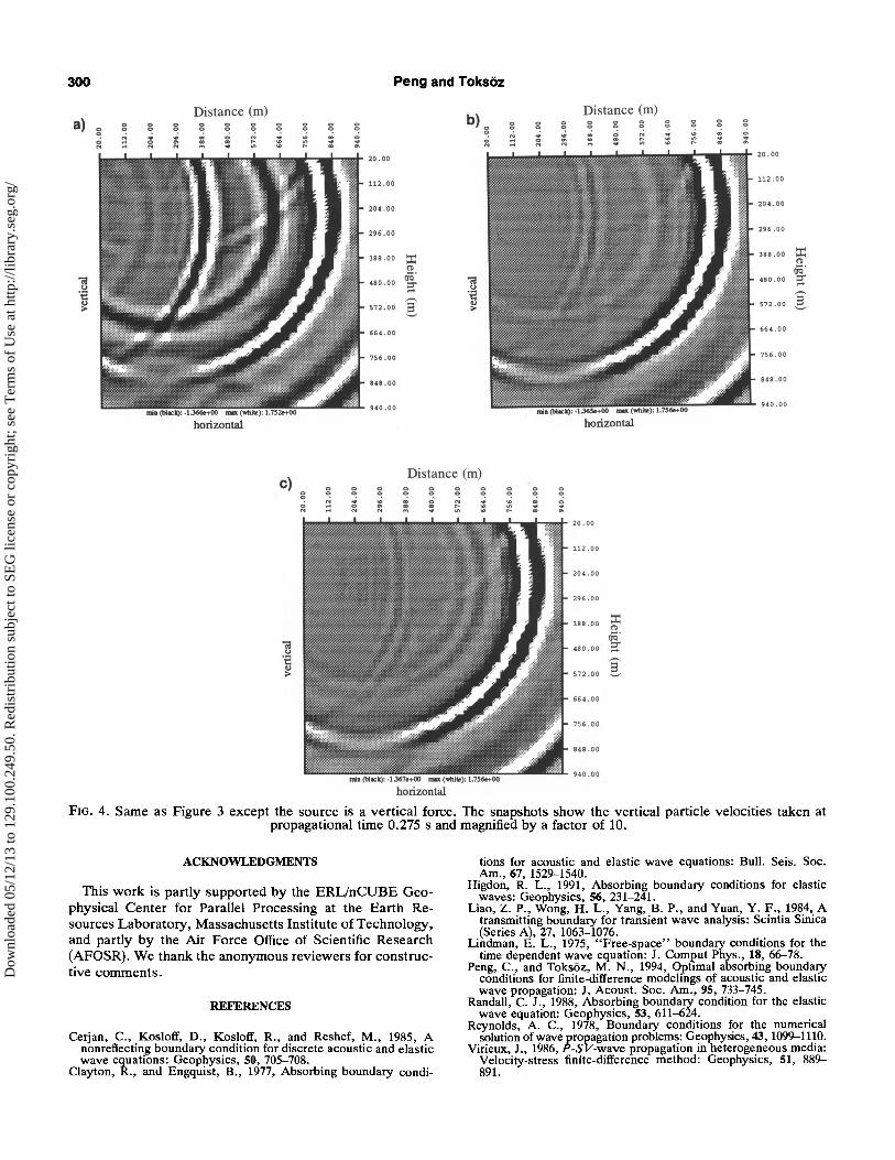
In the second example, as is shown in Figure 4, we use avertical force. The optimal absorbing boundary condition isdesigned for maximum absorption of incident S-waves at11.32 and 40.40 degrees. The first arrival near the lower-rightcorner is the direct P-wave and the one that follows is thedirect S -wave, All the other events are artificial ones causedby reflections from boundaries. Here the artificial reflection

FIG. 2. Elastic reflection coefficients (a) R sp and (b) R ss , asa function of the incidence angle for the optimal, Reynolds(1978), and Higdon (1991) absorbing boundary conditions.

conditions by using equation (18c) in Reynolds (1978) andequation (12) with (131 = cos 6+, 132 = cos 6-) in Higdon(1991), respectively. The reflection coefficient of the optimalabsorbing boundary condition has two additional zeros andis generally 10--20 dB less in magnitude than the Higdon'sabsorbing boundary condition at small angles of incidence.At large angle of incidence, Higdon's absorbing boundarycondition yields the same reflection coefficient as the optimalone. The Higdon absorbing boundary condition, in turn, hasa better performance by about 10-20 dB (less) over theReynolds boundary condition, except at an angle near graz­ing incidence. The P-wave to S-wave reflection coefficientshows similar behavior as the P-wave to P-wave reflectioncoefficient. By comparison with plots described by Reynolds(1978) and Higdon (1991), we find that the reflection coeffi­cients on a discrete finite-difference grid are different fromthose that are derived from an analytical boundary condi­tion. For example, in the continuous case the acousticreflection coefficient in both the Reynolds and Higdon ab­sorbing boundary conditions is zero at normal incidence 6 =odegrees and 6 = 6:!:, respectively, while this is no longerthe case on the discrete finite-difference grid.

Figure 2 shows the elastic S-wave to P-wave and S-wave toS-wave reflection coefficients of a particular design with 6 + =40.4 degrees and 6- = 11.32 degrees for a maximum absorp­tion of the incident S-wave. Again, the optimal absorbingboundary condition outperforms the others by reducing themagnitudes of the reflection coefficients by approximately10--20 dB. The Reynold's absorbing boundary condition yieldsa reflection coefficient whose amplitude exceeds 1.0 at angle ofincidence near 40 degrees, showing numerical instability inelastic wave modeling. The Higdon absorbing boundary con­dition is identical to the optimal one at large angles of inci­dence. However, at small angles of incidence, the optimalabsorbing boundary condition is much better.

NUMERICAL EXAMPLES

In the examples, we simulate elastic wave propagation inan unbounded homogeneous medium using a 3-D elasticfinite-difference method. The finite-difference code employsa stress-velocity formulation (Virieux, 1986) and is imple­mented on a nCUBE parallel computer. The medium prop­erties are: compressional velocity 0: = 3000 m/s, shearvelocity 13 = 2000 m/s, and density p = 2000 Kglm 3

•

The source function is a delayed Ricker wavelet (s(t)= (2Tr 2f J (t - to)2 - l)e-1I"

2N (t - to)2) with central fre­

quency fo = 20 Hz and time delay to = fo- 1• The size of the

3-D volume is 960 m in each dimension. The time step is I1t= 0.0005 s and the grid size is I1x = 10 m. The source is atcoordinates 240 m, 240 m, and 240 m (one quarter of theframe size of the snapshots from the upper-left corner ineach dimension). All six surfaces are absorbing boundarieswith either the optimal, Reynolds, or Higdon boundarycondition. The snapshots are shown are the vertical particlevelocities in thexz-plane aty = 240 m at propagational time0.30 s in the first example and at 0.275 s in the secondexample. The snapshots are blown up by a factor of 10 tomake reflections from the artificial boundaries visible.

In the first example, as is shown in Figure 3, we use anexplosive source. The optimal absorbing boundary condition

-10

-70

·80

enE·301:.9l~-40

8:5-50

~"" -60£

·70

-80

10

10

20

20

_Optimal

000 Higdon

H+ Reynold

30 40 50 60Incidence Angle (degree)

_Optimal

000 Higdon

+++ Reynold ,.-1'+~+++i=

+++

++

+

30 40 50 60Incidence Angle (degree)

70

70

80

80

+

+

+

90

90

Dow

nloa

ded

05/1

2/13

to 1

29.1

00.2

49.5

0. R

edis

trib

utio

n su

bjec

t to

SEG

lice

nse

or c

opyr

ight

; see

Ter

ms

of U

se a

t http

://lib

rary

.seg

.org

/

Optimal Absorbing Boundary Condition 299

with the optimal absorbing boundary condition (Figure 4c) isalmost the same as that with the Higdon absorbing boundarycondition in terms of maximum amplitude, and both of themare much better than the one with the Reynolds absorbingboundary condition. The artificial event that appears to be areflection from the upper-left corner is an out-of-plane ar­rival from the absorbing boundary y = o.

CONCLUSIONS

The optimal absorbing condition designed with thetechnique described in this note yields reflection co-

efficients about 10-20 dB less in magnitude than theHigdon absorbing condition and about 20-30 dB lessthan the Reynolds absorbing condition for a fixedextrapolation length that is two steps in both time andspace. Realistic 3-D elastic finite-difference modeling ofwave propagation on a parallel computer nCUBE-2 showsthat the optimal absorbing boundary condition is su­perior to those of Reynolds and Higdon. The fast algo­rithm enables one to compute the coefficients of theoptimal absorbing boundary condition accurately andefficiently.

Distance (m)

;;....--- H O. OO

156 .00

660&.00

296 .00

388 .00 ::t(1l

ciQ '4' 0 . 00 go

572 .00 ~

848 .00

204. 00

20 .00

112.00

ooo::

oo.......

o

~e-

oo.......

so.....

oo....~

~....'"

oo...o

'"

oo

'":::o

'"

b) g

Distance (m)0 0 0 0 0 0 0 00 ~ 0 0 0 ~

0 0.. .. 0 '" ... .. .. 0.. .. .. e-- .. ~ ... ::'" ~ ... ~ .. .. ..20 .00

112 .00

204 . 00

296 . 00

388 .00 ::t(1l

.e0 .00ciQ ';:r

572 .00 ~664 .00

7 56 .0 0

84'.00

940 .00

oo...o'"

oo

'":::a) g

o'"

c)

"§'ilo>

ooo

'"

o 0o 0

E ~

Distance (m)0 0 0 0 0 0 0 00 0 0 0 0 0 0 0

~.. :: '" ... .. .. 0.. e- .. ~ ... ...~ ... ~ .. e- .. ..

20 . 00

112 . 00

20 4 . 00

296 .00

::t388 .00

(1l

06 '::r....

4.10 .00 ,-...

2-572 .00

66" .00

756 .00

8U .00

HO .OO

FIG. 3. Snapshots of 3-D elastic finite-difference simulations on an nCUBE parallel computer, using the (a) Reynolds (1978), (b)Higdon (1991), and (c) optimal absorbing boundary conditions. An explosive source is used. The source is located at one quarterof the frame size from the upper-left corner in each dimension. The snapshots are the vertical particle velocities taken atpropagational time 0.30 s and magnified by a factor of 10.

Dow

nloa

ded

05/1

2/13

to 1

29.1

00.2

49.5

0. R

edis

trib

utio

n su

bjec

t to

SEG

lice

nse

or c

opyr

ight

; see

Ter

ms

of U

se a

t http

://lib

rary

.seg

.org

/

300

Distance (m)a) 0 0 0 0 0 0 0 0 0

~0 0 0 ~ 0 0 0 0 ~N . . 0 N . ·~ ;1 ~ :i: . .

~ ~ "' ·~ . r- ·

Peng and Toksoz

b) ~Distance (m)

~ ~0 s ~

0 0 0 00 0 0 0 0

N . . . 0 N · . .0 ~ 0 ~ . . e- · r-- .N ~ N N ~ . "' ·

00

0

~

20 .00

112 .00

20 4.00

296 .0 0

388 .00 ::r::C1>dQ'

uo.oo go,.-.,

572 .00 3'-'

664 . 00

1506. 00

848 .0 0

940 . 00

c)Distance (m)

0 ~0

~0 0 0 0 0 0

0 0 0 0 0 0 00

N . . . 0 N · . ·0 ~ 0 ~ . . ... · "' ·N ~ N N ~ . "' · ... ·00

:20 .00

112 .0 0

204 .00

296 .00

388 .0 0 ::r::C1>dQ'

480 .00 go,.-.,

572.00 2-664 . 0 0

756 . 00

848 . 00

940 . 00

FIG. 4. Same as Figure 3 except the source is a vertical force. The snapshots show the vertical particle velocities taken atpropagational time 0.275 s and magnified by a factor of 10.

ACKNOWLEDGMENTS

This work is partly supported by the ERL/nCUBE Geo­physical Center for Parallel Processing at the Earth Re­sources Laboratory, Massachusetts Institute of Technology,and partly by the Air Force Office of Scientific Research(AFOSR). We thank the anonymous reviewers for construc­tive comments.

REFERENCES

Cerjan, c., Kosloff, D., Kosloff, R., and Reshef, M., 1985, Anonreflecting boundary condition for discrete acoustic and elasticwave equations: Geophysics, 50, 705-708.

Clayton, R., and Engquist, B., 1977, Absorbing boundary condi-

tions for acoustic and elastic wave equations: Bull. Seis. Soc.Am., 67, 1529-1540.

Higdon, R. L., 1991, Absorbing boundary conditions for elasticwaves: Geophysics, 56, 231-241.

Liao, Z. P., Wong, H. L., Yang, B. P., and Yuan, Y. F., 1984, Atransmitting boundary for transient wave analysis: Scintia Sinica(Series A), 27, 1063-1076. .

Lindman, E. L., 1975, "Free-space" boundary conditions for thetime dependent wave equation: J. Comput Phys., 18, 66-78.

Peng, C., and Toksoz, M. N., 1994, Optimal absorbing boundaryconditions for finite-difference modelings of acoustic and elasticwave propagation: J. Acoust. Soc. Am., 95, 733-745.

Randall, C. J., 1988, Absorbing boundary condition for the elasticwave equation: Geophysics, 53, 611-624.

Reynolds, A. C., 1978, Boundary conditions for the numericalsolution of wave propagation problems: Geophysics, 43,1099--1110.

Virieux, J., 1986, PoSY-wave propagation in heterogeneous media:Velocity-stress finite-difference method: Geophysics, 51, 889­891.

Dow

nloa

ded

05/1

2/13

to 1

29.1

00.2

49.5

0. R

edis

trib

utio

n su

bjec

t to

SEG

lice

nse

or c

opyr

ight

; see

Ter

ms

of U

se a

t http

://lib

rary

.seg

.org

/

Optimal Absorbing Boundary Condition

APPENDIX

A FAST ALGORITHM

301

Let R z = cos Ai, I z = sin &, R; = cos ({t+ + {t_),

Ix = sin ({t+ + {t_), R y = -(cos {t+ + cos {t_), andI y = - (sin {t + + sin {t _ ). The coefficients {aij} in equation(1) are given by

alO =a12 ='Yi~)+'YH6) IJ.,

aOI = a21 = 'Y6~) + 'YW IJ.,

a02 = a20 = 'Y6rr + 'Y6~) IJ.,

_ (0) (1)all - 'Yll + 'Yll IJ.,

and

a22 = -1.

In the above equations,

'Yit)(1 - Rz)[(RxRz - IxIz) + (RxIz + RzIx) - (R z - I z)]

~

(1) __ 1 (1)'YOI - 2-'Y1O,

and

'Y(O) _ 'IJ'10 - ~ ,

<I>'Y

(O) - ­02 - ~'

where

~ = [Ry + Iy + 2Rz][(RxRz - IxIz)

+ (RxIz + RzIx) - (R z - I z))

+ [1 - R x - Ix][2 + (RyRz - IyIz)

+ (RyIz + RzIy »),

'IJ' = [1 + R z + (RyRz + IyIz) - (RyIz - RzIy)]

x [RxRz - IxIz) + (RxIz + RzIx) - R z + I z)

+ [Rz + I z - (RxRz + IxIz) - (RzIx - RxIz)]

x [2 + (RyRz - IyIz) + (RyIz + RzIy)],

<I> = [1 - R x - Ix][l + R; + (RyRz + IyIz)

- (RyIz - RzIy»)

- [Rz + I z - (RxRz + IxIz) - (RzIx - RxIz)],

and

2('Y (O)'Y (1) + 'Y(O)'Y (1) + 'Y(O)'Y (1» + 'Y(O)'Y (1)10 10 01 01 02 02 11 11

IJ. = - 2('Y(1)'Y(1) + 'Y(I)'Y(I) + 'Y(l)'Y(I» + 'Y(I)'Y(I)·10 10 01 01 02 02 11 11

Dow

nloa

ded

05/1

2/13

to 1

29.1

00.2

49.5

0. R

edis

trib

utio

n su

bjec

t to

SEG

lice

nse

or c

opyr

ight

; see

Ter

ms

of U

se a

t http

://lib

rary

.seg

.org

/