An Open-Source Microscopic Traffic Simulator

© LUSHPIX & COMSTOCK

IEEE INTELLIGENT TRANSPORTATION SYSTEMS MAGAZINE • 6 • FALL 2010 1939-1390/10/$26.00©2010IEEE1939-1390/10/$26.00©2010IEEE

Abstract–We present the interactive Java-based open-source traffic simulator available at www.traffic-simulation.de. In contrast to most closed-source commercial simulators, the focus is on investigating fundamental issues of traffic dynamics rather than simulating specific road networks. This includes testing theories for the spatiotemporal evolution of traffic jams, comparing and testing different microscopic traffic models, modeling the effects of driving styles and traffic rules on the efficiency and stability of traffic flow, and investi-gating novel ITS technologies such as adaptive cruise control, inter-vehicle and vehicle-infrastructure communication.

Digital Object Identifier 10.1109/MITS.2010.939208

Martin Treiber and Arne Kesting

Department of Transport and Traffic Sciences, Technische Universität Dresden,

Würzburger Str. 35, 01062 Dresden, Germany

E-mail: [email protected]

IEEE INTELLIGENT TRANSPORTATION SYSTEMS MAGAZINE • 7 • FALL 2010

1 Since further perturbations are inherently provoked by lane changes,

traffic can also break down without external action.2 The default parameter settings correspond to extremely unstable traffic.

For more realistic values, it would take even longer [4].

I. Introduction

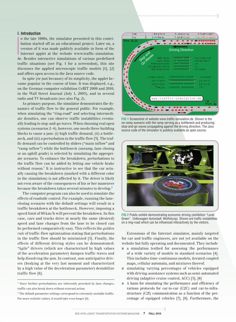
In the late 1990s, the simulator presented in this contri-bution started off as an educational project. Later on, a version of it was made publicly available in form of the Internet applet at the website www.traffic-simulation.

de. Besides interactive simulations of various predefined traffic situations (see Fig. 1 for a screenshot), this site discusses the applied microscopic traffic models [1], [2] and offers open access to the Java source code.

In spite (or just because) of its simplicity, the applet be-came popular in the course of time. It was displayed, e.g., on the German computer exhibition CeBIT 2009 and 2010, in the Wall Street Journal (July 1, 2005), and in several radio and TV broadcasts (see also Fig. 2).

As primary purpose, the simulator demonstrates the dy-namics of traffic flow to the general public. For example, when simulating the “ring-road” and selecting intermedi-ate densities, one can observe traffic instabilities eventu-ally leading to stop-and-go waves. When choosing real open systems (scenarios 2–4), however, one needs three building blocks to cause a jam: (i) high traffic demand, (ii) a bottle-neck, and (iii) a perturbation in the traffic flow [3]. The traf-fic demand can be controlled by sliders (“main inflow” and “ramp inflow”) while the bottleneck (onramp, lane closing or an uphill grade) is selected by simulating the appropri-ate scenario. To enhance the breakdown, perturbations to the traffic flow can be added by letting one vehicle brake without reason.1 It is instructive to see that the car actu-ally causing the breakdown (marked with a different color in the simulation) is not affected by it. The driver is likely not even aware of the consequences of his or her maneuver because the breakdown takes several minutes to develop.2

The computer program can also be used to simulate the effects of roadside control. For example, running the lane-closing scenario with the default settings will result in a traffic breakdown at the bottleneck. However, imposing a speed limit of 80 km/h will prevent the breakdown. In this case, cars and trucks drive at nearly the same (desired) speed and lane changes from the lane to be closed can be performed comparatively easy. This reflects the golden rule of traffic-flow optimization stating that perturbations in the traffic flow should be minimized [5]. Finally, the effects of different driving styles can be demonstrated: “Agile” drivers (which are characterized by high values of the acceleration parameter) dampen traffic waves and help dissolving the jam. In contrast, non-anticipative driv-ers (braking at the very last moment and characterized by a high value of the deceleration parameter) destabilize traffic flow [6].

Extensions of the Internet simulator, mainly targeted for car and traffic engineers, are not yet available on the website but fully operating and documented. They include

■ a simulation testbed for assessing the performance of a wide variety of models in standard scenarios [4]. This includes time-continuous models, iterated coupled maps, cellular automata, and mixtures thereof.

■ simulating varying percentages of vehicles equipped with driving-assistance systems such as semi-automated driving (adaptive cruise control, ACC) [5], [6]

■ A basis for simulating the performance and efficiency of various protocols for car-to-car (C2C) and car-to-infra-structure (C2I) communication as a function of the per-centage of equipped vehicles [7], [8]. Furthermore, the

Driving Direction

Stop

and

Go

Wav

es

www.traffic−simulation.de

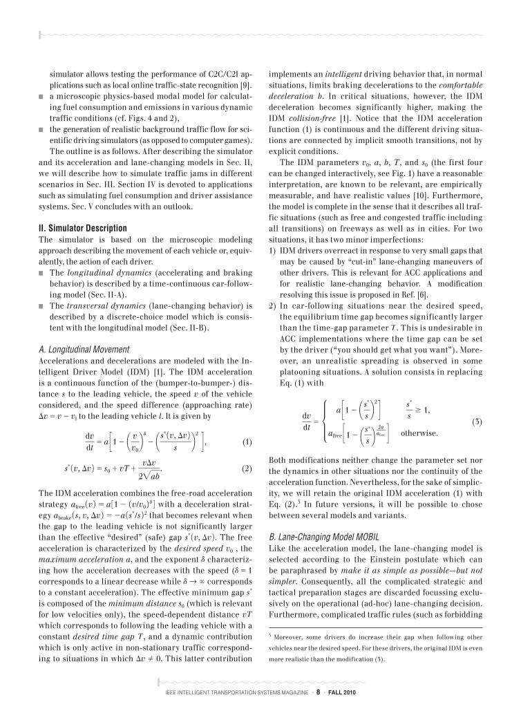
FIG 1 Screenshot of website www.traffic-simulation.de. Shown is the on-ramp scenario with the ramp serving as a bottleneck and producing stop-and-go waves propagating against the driving direction. The Java source code of the simulator is publicly available as open source.

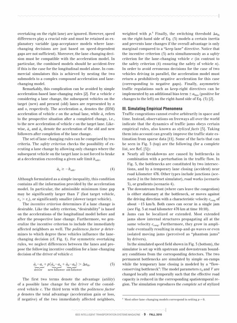
FIG 2 Public exhibit demonstrating economic driving (exhibition “Level Green”, Volkswagen Autostadt, Wolfsburg). Shown are traffic instabilities on a ring-road which can be influenced interactively by the visitors.


simulator allows testing the performance of C2C/C2I ap-plications such as local online traffic-state recognition [9].

■ a microscopic physics-based modal model for calculat-ing fuel consumption and emissions in various dynamic traffic conditions (cf. Figs. 4 and 2),

■ the generation of realistic background traffic flow for sci-entific driving simulators (as opposed to computer games).The outline is as follows. After describing the simulator

and its acceleration and lane-changing models in Sec. II, we will describe how to simulate traffic jams in different scenarios in Sec. III. Section IV is devoted to applications such as simulating fuel consumption and driver assistance systems. Sec. V concludes with an outlook.

II. Simulator DescriptionThe simulator is based on the microscopic modeling approach describing the movement of each vehicle or, equiv-alently, the action of each driver.

■ The longitudinal dynamics (accelerating and braking behavior) is described by a time-continuous car-follow-ing model (Sec. II-A).

■ The transversal dynamics (lane-changing behavior) is described by a discrete-choice model which is consis-tent with the longitudinal model (Sec. II-B).

A. Longitudinal MovementAccelerations and decelerations are modeled with the In-telligent Driver Model (IDM) [1]. The IDM acceleration is a continuous function of the (bumper-to-bumper-) dis-tance s to the leading vehicle, the speed v of the vehicle considered, and the speed difference (approaching rate) Dv 5 v 2 vl to the leading vehicle l. It is given by

dvdt

5 a c1 2 a vv0bd

2 as* 1v, Dv 2s

b2

d , (1)

s* 1v, Dv 2 5 s0 1 vT 1vDv

2"ab. (2)

The IDM acceleration combines the free-road acceleration strategy afree 1v 2 5 a 31 2 1v/v0 2 d 4 with a deceleration strat-egy abrake 1s, v, Dv 2 5 2a 1s*/s 2 2 that becomes relevant when the gap to the leading vehicle is not significantly larger than the effective “desired” (safe) gap s* 1v, Dv 2 . The free acceleration is characterized by the desired speed v0 , the maximum acceleration a, and the exponent d characteriz-ing how the acceleration decreases with the speed (d 5 1 corresponds to a linear decrease while d S ` corresponds to a constant acceleration). The effective minimum gap s* is composed of the minimum distance s0 (which is relevant for low velocities only), the speed-dependent distance vT which corresponds to following the leading vehicle with a constant desired time gap T , and a dynamic contribution which is only active in non-stationary traffic correspond-ing to situations in which Dv 2 0. This latter contribution

implements an intelligent driving behavior that, in normal situations, limits braking decelerations to the comfortable deceleration b. In critical situations, however, the IDM deceleration becomes significantly higher, making the IDM collision-free [1]. Notice that the IDM acceleration function (1) is continuous and the different driving situa-tions are connected by implicit smooth transitions, not by explicit conditions.

The IDM parameters v0, a, b, T , and s0 (the first four can be changed interactively, see Fig. 1) have a reasonable interpretation, are known to be relevant, are empirically measurable, and have realistic values [10]. Furthermore, the model is complete in the sense that it describes all traf-fic situations (such as free and congested traffic including all transitions) on freeways as well as in cities. For two situations, it has two minor imperfections: 1) IDM drivers overreact in response to very small gaps that

may be caused by “cut-in” lane-changing maneuvers of other drivers. This is relevant for ACC applications and for realistic lane-changing behavior. A modification resolving this issue is proposed in Ref. [6].

2) In car-following situations near the desired speed, the equilibrium time gap becomes significantly larger than the time-gap parameter T . This is undesirable in ACC implementations where the time gap can be set by the driver (“you should get what you want”). More-over, an unrealistic spreading is observed in some platooning situations. A solution consists in replacing Eq. (1) with

dvdt

5 µ a c1 2 as*

sb2 d

s*

s$ 1,

afree c1 2 as*

s b 2aafree d otherwise.

(3)

Both modifications neither change the parameter set nor the dynamics in other situations nor the continuity of the acceleration function. Nevertheless, for the sake of simplic-ity, we will retain the original IDM acceleration (1) with Eq. (2).3 In future versions, it will be possible to chose between several models and variants.

B. Lane-Changing Model MOBILLike the acceleration model, the lane-changing model is selected according to the Einstein postulate which can be paraphrased by make it as simple as possible—but not simpler. Consequently, all the complicated strategic and tactical preparation stages are discarded focussing exclu-sively on the operational (ad-hoc) lane-changing decision. Furthermore, complicated traffic rules (such as forbidding

3 Moreover, some drivers do increase their gap when following other

vehicles near the desired speed. For these drivers, the original IDM is even

more realistic than the modification (3).


overtaking on the right lane) are ignored. However, speed differences play a crucial role and must be retained as ex-planatory variable (gap-acceptance models where lane-changing decisions are just based on speed- dependent gaps are not sufficient). Moreover, the lane-changing deci-sion must be compatible with the acceleration model. In particular, the combined models should be accident-free if this is the case for the longitudinal model alone. In com-mercial simulators this is achieved by nesting the two submodels to a complex compound acceleration and lane-changing model.

Remarkably, this complication can be avoided by simple acceleration-based lane-changing rules [2]. For a vehicle c considering a lane change, the subsequent vehicles on the target (new) and present (old) lanes are represented by n and o, respectively. The acceleration ac denotes the (IDM) acceleration of vehicle c on the actual lane, while a| c refers to the prospective situation after a completed change, i.e., to the new acceleration of vehicle c on the target lane. Like-wise, a|o and a|n denote the acceleration of the old and new followers after completion of the lane change.

The set of lane-changing rules can be comprised by two criteria. The safety criterion checks the possibility of ex-ecuting a lane change by allowing only changes where the subsequent vehicle on the target lane is not forced to brake at a deceleration exceeding a given safe limit bsafe,

a|n $ 2bsafe. (4)

Although formulated as a simple inequality, this condition contains all the information provided by the acceleration model. In particular, the admissible minimum time gap may be significantly larger than T (fast target vehicle, vn . vc), or significantly smaller (slower target vehicle).

The incentive criterion determines if a lane change is desirable. Like the safety criterion, “desirability” is based on the accelerations of the longitudinal model before and after the prospective lane change. Furthermore, we gen-eralize the incentive criterion to include the immediately affected neighbors as well. The politeness factor p deter-mines to which degree these vehicles influence the lane-changing decision (cf. Fig. 1). For symmetric overtaking rules, we neglect differences between the lanes and pro-pose the following incentive condition for a lane-changing decision of the driver of vehicle c:

a|c2ac 1 p 1a|n2an 1 a|02a0 2 . Dath. (5)

The first two terms denote the advantage (utility) of a possible lane change for the driver of the consid-ered vehicle c. The third term with the politeness factor p denotes the total advantage (acceleration gain or loss, if negative) of the two immediately affected neighbors,

weighted with p.4 Finally, the switching threshold Dath on the right-hand side of Eq. (5) models a certain inertia and prevents lane changes if the overall advantage is only marginal compared to a “keep lane” directive. Notice that the incentive criterion (5) acts simultaneously as a safety criterion for the lane-changing vehicle c (in contrast to the safety criterion (4) ensuring the safety of vehicle n). In order to avoid erroneous decisions for the case of two vehicles driving in parallel, the acceleration model must return a prohibitively negative acceleration for this case (corresponding to negative gaps). Finally, asymmetric traffic regulations such as keep-right directives can be implemented by an additional bias term 6 abias (positive for changes to the left) on the right-hand side of Eq. (5) [2].

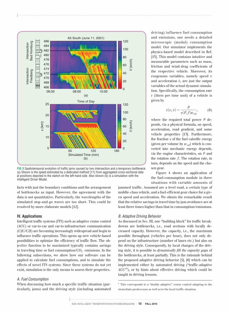
III. Simulating Empirical PhenomenaTraffic congestions cannot evolve arbitrarily in space and time. Instead, observations on freeways all over the world indicate that the dynamics of traffic jams obeys certain empirical rules, also known as stylized facts [3]. Taking them into account can greatly improve the traffic state es-timation from sparse data [11]. Some of the facts that can be seen in Fig. 3 (top) are the following (for a complete list, see Ref. [3]):

■ Nearly all breakdowns are caused by bottlenecks in combination with a perturbation in the traffic flow. In Fig. 3, the bottlenecks are constituted by two intersec-tions, and by a temporary lane closing (accident) near road kilometer 476. Other types include junctions (sce-nario 2 in the Internet simulator), road works (scenario 3), or gradients (scenario 4).

■ The downstream front (where cars leave the congestion) is either stationary at the bottleneck, or moves against the driving direction with a characteristic velocity ccong of about 215 km/h. Both cases can occur in a single jam (see Fig. 3 at road kilometer 476 km at time 10:10).

■ Jams can be localized or extended. Most extended jams show internal structures propagating all at the same velocity ccong. Furthermore, they grow in ampli-tude eventually resulting in stop-and-go waves or even isolated moving jams (perceived as “phantom jams” by drivers).In the simulated speed field shown in Fig. 3 (bottom), the

simulator is set up with upstream and downstream bound-ary conditions from the corresponding detectors. The two permanent bottlenecks are simulated by simple on-ramps while the temporary lane closing is modeled by a “flow-conserving bottleneck”: The model parameters v0 and T are changed locally and temporally such that the effective road capacity is reduced in the corresponding spatiotemporal re-gion. The simulation reproduces the complete set of stylized

b b b driver new follower old follower

4 Most other lane-changing models correspond to setting p 5 0.


facts with just the boundary conditions and the arrangement of bottlenecks as input. However, the agreement with the data is not quantitative. Particularly, the wavelengths of the simulated stop-and-go waves are too short. This could be resolved by more elaborate models [12].

IV. ApplicationsIntelligent traffic systems (ITS) such as adaptive cruise control (ACC) or car-to-car and car-to-infrastructure communication (C2C/C2I) are becoming increasingly widespread and begin to influence traffic operations. This opens up new vehicle-based possibilities to optimize the efficiency of traffic flow. The ob-jective function to be maximized typically contains savings in traveling time or fuel consumption/CO2 emissions. In the following subsections, we show how our software can be applied to calculate fuel consumptions, and to simulate the effects of novel ITS systems. Since these systems do not yet exist, simulation is the only means to assess their properties.

A. Fuel ConsumptionWhen discussing how much a specific traffic situation (par-ticularly, jams) and the driving style (including automated

driving) influence fuel consumption and emissions, one needs a detailed microscopic (modal) consumption model. Our simulator implements the physics-based model described in Ref. [13]. This model contains intuitive and measurable parameters such as mass, friction and wind-drag coefficients of the respective vehicle. Moreover, its exogenous variables, namely speed v and acceleration v

#, are just the output

variables of the actual dynamic simula-tion. Specifically, the consumption rate c# (liters per time unit) of a vehicle is given by

c# 1v, v

# 2 5P

g 1P, f 2wcal, (6)

where the required total power P de-pends, via a physical formula, on speed, acceleration, road gradient, and some vehicle properties [13]. Furthermore, the fraction g of the fuel calorific energy (given per volume by wcal) which is con-verted into mechanic energy depends, via the engine characteristics, on P and the rotation rate f . The rotation rate, in turn, depends on the speed and the cho-sen gear.

Figure 4 shows an application of the fuel-consumption module in three situations with variable amounts of

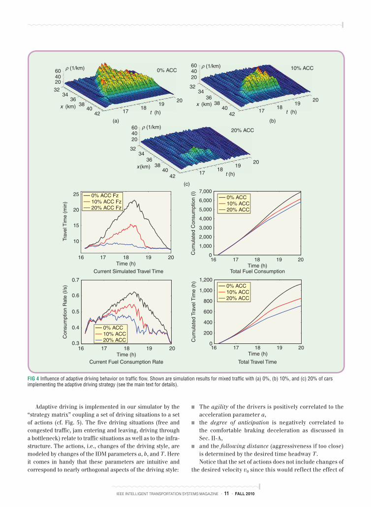
jammed traffic. Assumed are a level road, a certain type of middle-class vehicle, and a fuel-efficient gear choice for a giv-en speed and acceleration. We obtain the remarkable result that the relative savings in travel time by jam avoidance are at least three times higher than that in consumption/emissions.

B. Adaptive Driving BehaviorAs discussed in Sec. III, one “building block” for traffic break-downs are bottlenecks, i.e., road sections with locally de-creased capacity. However, the capacity, i.e., the maximum possible throughput (vehicles per hour), does not only de-pend on the infrastructure (number of lanes etc.) but also on the driving style. Consequently, by local changes of the driv-ing style, it is possible to dynamically fill the capacity gaps of the bottlenecks, at least partially. This is the rationale behind the proposed adaptive driving behavior [5], [6] which can be implemented either by automated driving (“traffic-adaptive ACC”5), or by hints about effective driving which could be taught in driving lessons.

A5 South (June 11, 2001)

06:00 08:00 10:00

Time of Day

466

468

470

472

474

476

478

480

482

484

486

0

20

40

60

80

100

120

V (

km

/h)

V (

km

/h)

0

20

40

60

80

100

120

Inte

rsection

Fri

edberg

Inte

rsection

Bad H

om

burg

60 120 180

Simulated Time (min)

10

5

15

20

25

x (k

m)

(a)

(b)

FIG 3 Spatiotemporal evolution of traffic jams caused by two intersection and a temporary bottleneck. (a) Shown is the speed estimated by a dedicated method [11] from aggregated cross-sectional data at positions depicted in the sketch on the left-hand side. Also shown (b) is a simulation with the Intelligent Driver Model.

5 This corresponds to a “doubly adaptive” cruise control adapting to the

immediate predecessor as well as to the local traffic situation.


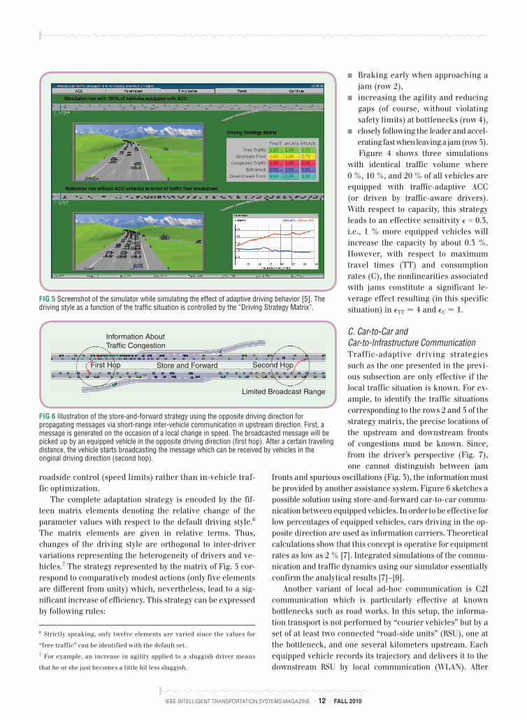
Adaptive driving is implemented in our simulator by the “strategy matrix” coupling a set of driving situations to a set of actions (cf. Fig. 5). The five driving situations (free and congested traffic, jam entering and leaving, driving through a bottleneck) relate to traffic situations as well as to the infra-structure. The actions, i.e., changes of the driving style, are modeled by changes of the IDM parameters a, b, and T . Here it comes in handy that these parameters are intuitive and correspond to nearly orthogonal aspects of the driving style:

■ The agility of the drivers is positively correlated to the acceleration parameter a,

■ the degree of anticipation is negatively correlated to the comfortable braking deceleration as discussed in Sec. II-A,

■ and the following distance (aggressiveness if too close) is determined by the desired time headway T .Notice that the set of actions does not include changes of

the desired velocity v0 since this would reflect the effect of

0

200

400

600

800

1,000

1,200

16 17 18 19 20

Cum

ula

ted T

rave

l Tim

e (

h)

Time (h)

16 17 18 19 20

Time (h)

10

15

20

25

16 17 18 19 20

Tra

vel T

ime (

min

)

Time (h)

16 17 18 19 20Time (h)

0% ACC10% ACC20% ACC


0% ACC Fz10% ACC Fz20% ACC Fz


0.7

0.6

0.5

0.4

0.3

Consum

ption R

ate

(l/s)

0

1,000

2,000

3,000

4,000

5,000

6,000

7,000C

um

ula

ted C

onsum

ption (

l)

ρ (1/km)

ρ (1/km)

ρ (1/km)0% ACC 10% ACC

20% ACC

Current Simulated Travel Time

Current Fuel Consumption Rate

Total Fuel Consumption

Total Travel Time

x (km)

x (km)

x (km)

t (h)

604020

3234

3638

4042 17

1819

20

t (h)

604020

3234

3638

4042

1718

1920

t (h)

604020

3234

3638

4042

1718

1920

(a) (b)

(c)

FIG 4 Influence of adaptive driving behavior on traffic flow. Shown are simulation results for mixed traffic with (a) 0%, (b) 10%, and (c) 20% of cars implementing the adaptive driving strategy (see the main text for details).


roadside control (speed limits) rather than in-vehicle traf-fic optimization.

The complete adaptation strategy is encoded by the fif-teen matrix elements denoting the relative change of the parameter values with respect to the default driving style.6 The matrix elements are given in relative terms. Thus, changes of the driving style are orthogonal to inter-driver variations representing the heterogeneity of drivers and ve-hicles.7 The strategy represented by the matrix of Fig. 5 cor-respond to comparatively modest actions (only five elements are different from unity) which, nevertheless, lead to a sig-nificant increase of efficiency. This strategy can be expressed by following rules:

■ Braking early when approaching a jam (row 2),

■ increasing the agility and reducing gaps (of course, without violating safety limits) at bottlenecks (row 4),

■ closely following the leader and accel-erating fast when leaving a jam (row 5).Figure 4 shows three simulations

with identical traffic volume where 0 %, 10 %, and 20 % of all vehicles are equipped with traffic-adaptive ACC (or driven by traffic-aware drivers). With respect to capacity, this strategy leads to an effective sensitivity P 5 0.3,i.e., 1 % more equipped vehicles will increase the capacity by about 0.3 %. However, with respect to maximum travel times (TT) and consumption rates (C), the nonlinearities associated with jams constitute a significant le-verage effect resulting (in this specific situation) in PTT < 4 and PC < 1.

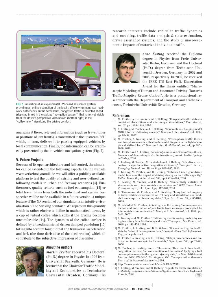
C. Car-to-Car and Car-to-Infrastructure CommunicationTraffic-adaptive driving strategies such as the one presented in the previ-ous subsection are only effective if the local traffic situation is known. For ex-ample, to identify the traffic situations corresponding to the rows 2 and 5 of the strategy matrix, the precise locations of the upstream and downstream fronts of congestions must be known. Since, from the driver’s perspective (Fig. 7), one cannot distinguish between jam

fronts and spurious oscillations (Fig. 3), the information must be provided by another assistance system. Figure 6 sketches a possible solution using store-and-forward car-to-car commu-nication between equipped vehicles. In order to be effective for low percentages of equipped vehicles, cars driving in the op-posite direction are used as information carriers. Theoretical calculations show that this concept is operative for equipment rates as low as 2 % [7]. Integrated simulations of the commu-nication and traffic dynamics using our simulator essentially confirm the analytical results [7]–[9].

Another variant of local ad-hoc communication is C2I communication which is particularly effective at known bottlenecks such as road works. In this setup, the informa-tion transpor t is not performed by “courier vehicles” but by a set of at least two connected “road-side units” (RSU), one at the bottleneck, and one several kilometers upstream. Eac h equipped vehicle records its trajectory and delivers it to the downstream RSU by local communication (WLAN). After

FIG 5 Screenshot of the simulator while simulating the effect of adaptive driving behavior [5]. The driving style as a function of the traffic situation is controlled by the “Driving Strategy Matrix”.

Information About

Traffic Congestion

Store and Forward

Limited Broadcast Range

Traffic Congestion

Store and Forward

Limited Broadcast Range

Second HopFirst Hop

FIG 6 Illustration of the store-and-forward strategy using the opposite driving direction for propagating messages via short-range inter-vehicle communication in upstream direction. First, a message is generated on the occasion of a local change in speed. The broadcasted message will be picked up by an equipped vehicle in the opposite driving direction (first hop). After a certain traveling distance, the vehicle starts broadcasting the message which can be received by vehicles in the original driving direction (second hop).

6 Strictly speaking, only twelve elements are varied since the values for

“free traffic” can be identified with the default set.7 For example, an increase in agility applied to a sluggish driver means

that he or she just becomes a little bit less sluggish.


analyzing it there, relevant information (such as travel times or positions of jam fronts) is transmitted to the upstream RSU which, in turn, delivers it to passing equipped vehicles by local communication. Finally, the information can be graphi-cally presented by the in-vehicle navigation system (Fig. 7).

V. Future ProjectsBecause of its open architecture and full control, the simula-tor can be extended in the following aspects. On the website www.verkehrsdynamik.de we will offer a publicly available platform to test the quality of existing and user-defined car-following models in urban and freeway scenarios [4]. Fur-thermore, quality criteria such as fuel consumption [13] or total travel times from bot h the individual and system per-spective will be made available in a future version. A unique feature of the 3D version of our simulator is an intuitive visu-alization of the “driving comfo rt”. We represent this quantity which is rather elusive to define in mathematical terms, by a cup of virtual coffee which spills if the driving becomes uncomfortable [14]. The dynamics of the coffee su rface is defined by a twodimensional driven damped pendulum [15] taking into account longitudinal and transversal acceleration and jerk (the time derivative of the acceleration) which all contribut e to the subjective impression of discomfort.

About the AuthorsMartin Treiber received his Doctoral (Ph.D.) degree in Physics in 1996 from Universität Bayreuth, Germany. He is lecturer at the Chair for Traffic Model-ing and Econometrics at Technische Universität Dresden, Germany. His

research interests include vehicular traffic dynamics and modeling, traffic data analysis & state estimation, driver assistance systems, and the study of macroeco-nomic impacts of motorized individual traffic.

Arne Kesting received the Diploma degree in Physics from Freie Univer-sität Berlin, Germany, and the Doctoral (Ph.D.) degree from Technische Uni-versität Dresden, Germany, in 2002 and 2008, respectively. In 2009, he received the IEEE ITS Best Ph.D. Dissertation Award for the thesis entitled “Micro-

scopic Modeling of Human and Automated Driving: Towards Traffic-Adaptive Cruise Control”. He is a postdoctoral re-searcher with the Departement of Transport and Traffic Sci-ences, Technische Universität Dresden, Germany.

References[1] M. Treiber, A. Hennecke, and D. Helbing, “Congested traffic states in

empirical observations and microscopic simulations,” Phys. Rev. E, vol. 62, pp. 1805–1824, 2000.

[2] A. Kesting, M. Treiber, and D. Helbing, “General lane-changing model MOBIL for car-following models,” Transport. Res. Record, vol. 1999, pp. 86–94, 2007.

[3] M. Treiber, A. Kesting, and D. Helbing, “Three-phase traffic theory and two-phase models with a fundamental diagram in the light of em-pirical stylized facts,” Transport. Res. B, Methodol., vol. 44, pp. 983–1000, 2010.

[4] M. Treiber and A. Kesting, Verkehrsdynamik und-Simulation—Daten, Modelle und Anwendungen der Verkehrsflussdynamik. Berlin: Spring-er-Verlag, 2010.

[5] A. Kesting, M. Treiber, M. Schönhof, and D. Helbing, “Adaptive cruise control design for active congestion avoidance,” Transport. Res. C, Emerging Technol., vol. 16, no. 6, pp. 668–683, 2008.

[6] A . Kesting, M. Treiber, and D. Helbing, “Enhanced intelligent driver model to access the impact of driving strategies on traffic capacity,” Philos. Trans. Royal Soc. A, vol. 368, pp. 4585–4605, 2010.

[7] A . Kesting, M. Treiber, and D. Helbing, “Connectivity statistics of store-and-forward inter-vehicle communication,” IEEE Trans. Intell. Transport. Syst., vol. 11, no. 1, pp. 172–181, 2010.

[8] C . Thiemann, M. Treiber, and A. Kesting, “Longitudinal hopping in inter-vehicle communication: Theory and simulations on mod-eled and empirical trajectory data,” Phys. Rev. E, vol. 78, p. 036102, 2008.

[9] M . Schönhof, M. Treiber, A. Kesting, and D. Helbing, “Autonomous de-tection and anticipation of jam fronts from messages propagated by intervehicle communication,” Transport. Res. Record, vol. 1999, pp. 3–12, 2007.

[10] A. Kesting and M. Treiber, “Calibrating car-following models by us-ing trajectory data: Methodological study,” Transport. Res. Record, vol. 2088, pp. 148–156, 2008.

[11] M. Treiber, A. Kesting, and R. E. Wilson, “Reconstructing the traffic state by fusion of heterogenous data,” Comput. Aided Civil Infrastruct. Eng., to be published.

[12] M. Treiber, A. Kesting, and D. Helbing, “Delays, inaccuracies and an-ticipation in microscopic traffic models,” Phys. A, vol. 360, pp. 71–88, 2006.

[13] M. Treiber, A. Kesting, and C. Thiemann, “How much does traffic congestion increase fuel consumption and emissions? Applying a fuel consumption model to the ngsim trajectory data,” in Proc. TRB Annual Meeting 2008 CD-ROM. Washington, DC: Transportation Research Board of the National Academies, 2008.

[14] http://www.youtube.com/watch?v=m9eELZCW4Ys [15] A. Kesting, M. Treiber, and D. Helbing, “Agents for traffic simulation,”

in Multi-Agent Systems: Simulation and Applications. New York: Taylor and Francis, 2008.

FIG 7 Simulation of an experimental C2I-based assistance system providing an online estimation of the local traffic environment near road-work bottlenecks. In the screenshot, congested traffic is detected ahead (depicted in red in the stylized “navigation system”) that is not yet visible from the driver’s perspective. Also shown (bottom right) is the “coffeemeter” visualizing the driving comfort.

Documents

An Open-Source Microscopic Traffic Simulator