This article was downloaded by: [The UC Irvine Libraries]On: 21 January 2015, At: 12:42Publisher: Taylor & FrancisInforma Ltd Registered in England and Wales Registered Number: 1072954 Registeredoffice: Mortimer House, 37-41 Mortimer Street, London W1T 3JH, UK

Click for updates

International Journal of RemoteSensingPublication details, including instructions for authors andsubscription information:http://www.tandfonline.com/loi/tres20

An object-based approach forverification of precipitation estimationJ. Lia, K. Hsub, A. AghaKouchakb & S. Sorooshianb

a Department of Geosciences and Environment, California StateUniversity Los Angeles, Los Angeles, CA, USAb Center for Hydrometeorology and Remote Sensing, Departmentof Civil & Environmental Engineering, University of CaliforniaIrvine, Irvine, CA, USAPublished online: 19 Jan 2015.

To cite this article: J. Li, K. Hsu, A. AghaKouchak & S. Sorooshian (2015) An object-based approachfor verification of precipitation estimation, International Journal of Remote Sensing, 36:2, 513-529,DOI: 10.1080/01431161.2014.999170

To link to this article: http://dx.doi.org/10.1080/01431161.2014.999170

PLEASE SCROLL DOWN FOR ARTICLE

Taylor & Francis makes every effort to ensure the accuracy of all the information (the“Content”) contained in the publications on our platform. However, Taylor & Francis,our agents, and our licensors make no representations or warranties whatsoever as tothe accuracy, completeness, or suitability for any purpose of the Content. Any opinionsand views expressed in this publication are the opinions and views of the authors,and are not the views of or endorsed by Taylor & Francis. The accuracy of the Contentshould not be relied upon and should be independently verified with primary sourcesof information. Taylor and Francis shall not be liable for any losses, actions, claims,proceedings, demands, costs, expenses, damages, and other liabilities whatsoever orhowsoever caused arising directly or indirectly in connection with, in relation to or arisingout of the use of the Content.

This article may be used for research, teaching, and private study purposes. Anysubstantial or systematic reproduction, redistribution, reselling, loan, sub-licensing,systematic supply, or distribution in any form to anyone is expressly forbidden. Terms &

Conditions of access and use can be found at http://www.tandfonline.com/page/terms-and-conditions

Dow

nloa

ded

by [

The

UC

Irv

ine

Lib

rari

es]

at 1

2:42

21

Janu

ary

2015

An object-based approach for verification of precipitation estimation

J. Lia*, K. Hsub, A. AghaKouchakb, and S. Sorooshianb

aDepartment of Geosciences and Environment, California State University Los Angeles,Los Angeles, CA, USA; bCenter for Hydrometeorology and Remote Sensing, Department of Civil

& Environmental Engineering, University of California Irvine, Irvine, CA, USA

(Received 4 July 2014; accepted 27 October 2014)

Verification has become an integral component in the development of precipitationalgorithms used in satellite-based precipitation products and evaluation of numericalweather prediction models. A number of object-based verification methods have beendeveloped to quantify the errors related to spatial patterns and placement of precipita-tion. In this study, an image processing technique known as watershed transformation,capable of detecting closely spaced, but separable precipitation areas, is adopted in theobject-based approach. Several key attributes of the segmented precipitation objectsare selected and interest values of those attributes are estimated based on the distancemeasurement of the estimated and reference images. An overall interest score isestimated from all the selected attributes and their interest values. The proposedobject-based approach is implemented to validate satellite-based precipitation estima-tion against ground radar observations. The results indicate that the watershed seg-mentation technique is capable of separating the closely spaced local-scaleprecipitation areas. In addition, three verification metrics, including the object-basedfalse alarm ratio, object-based missing ratio, and overall interest score, reveal the skillof precipitation estimates in depicting the spatial and geometric characteristics of theprecipitation structure against observations.

1. Introduction

Accurate representation of observed precipitation spatial patterns and structures is essen-tial for hydrologic applications. It has been noted that the spatial variability of precipita-tion has a major impact on the accuracy of modelled runoff volumes (Faurès et al. 1995;Goodrich et al. 1995). Especially in distributed hydrological modelling, the spatialpatterns and locations of precipitation events are important to describe the spatial hetero-geneity of precipitation (Foufoula-Georgiou and Vuruputur 2001).

In the last decade, satellite-based precipitation products and numerical weather prediction(NWP) models have provided precipitation estimates and forecasts, respectively, with highspatial and temporal resolution suitable for hydrologicmodelling and watershedmanagement.However, the quality of the simulated precipitation datasets is a vital factor in the decision touse these estimates for practical applications. Therefore, it is imperative that verification be anintegral component of precipitation algorithms and dataset development.

Several coordinated verification activities have been established to evaluate the accu-racy of precipitation estimation against ground observations, such as ground radar and raingauge data (Adler et al. 2001; AghaKouchak et al. 2012; AghaKouchak, Behrangi, et al.2011; Arkin and Turk 2006; Arkin and Xie 1994; Colle, Olson, and Tongue 2003; Ebert,

*Corresponding author. Email: Jingjing.Li@calstatela.edu

International Journal of Remote Sensing, 2015Vol. 36, No. 2, 513–529, http://dx.doi.org/10.1080/01431161.2014.999170

© 2015 Taylor & Francis

Dow

nloa

ded

by [

The

UC

Irv

ine

Lib

rari

es]

at 1

2:42

21

Janu

ary

2015

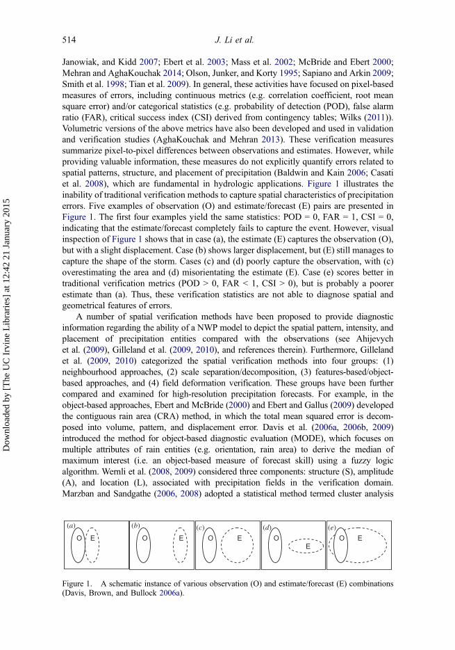
Janowiak, and Kidd 2007; Ebert et al. 2003; Mass et al. 2002; McBride and Ebert 2000;Mehran and AghaKouchak 2014; Olson, Junker, and Korty 1995; Sapiano and Arkin 2009;Smith et al. 1998; Tian et al. 2009). In general, these activities have focused on pixel-basedmeasures of errors, including continuous metrics (e.g. correlation coefficient, root meansquare error) and/or categorical statistics (e.g. probability of detection (POD), false alarmratio (FAR), critical success index (CSI) derived from contingency tables; Wilks (2011)).Volumetric versions of the above metrics have also been developed and used in validationand verification studies (AghaKouchak and Mehran 2013). These verification measuressummarize pixel-to-pixel differences between observations and estimates. However, whileproviding valuable information, these measures do not explicitly quantify errors related tospatial patterns, structure, and placement of precipitation (Baldwin and Kain 2006; Casatiet al. 2008), which are fundamental in hydrologic applications. Figure 1 illustrates theinability of traditional verification methods to capture spatial characteristics of precipitationerrors. Five examples of observation (O) and estimate/forecast (E) pairs are presented inFigure 1. The first four examples yield the same statistics: POD = 0, FAR = 1, CSI = 0,indicating that the estimate/forecast completely fails to capture the event. However, visualinspection of Figure 1 shows that in case (a), the estimate (E) captures the observation (O),but with a slight displacement. Case (b) shows larger displacement, but (E) still manages tocapture the shape of the storm. Cases (c) and (d) poorly capture the observation, with (c)overestimating the area and (d) misorientating the estimate (E). Case (e) scores better intraditional verification metrics (POD > 0, FAR < 1, CSI > 0), but is probably a poorerestimate than (a). Thus, these verification statistics are not able to diagnose spatial andgeometrical features of errors.

A number of spatial verification methods have been proposed to provide diagnosticinformation regarding the ability of a NWP model to depict the spatial pattern, intensity, andplacement of precipitation entities compared with the observations (see Ahijevychet al. (2009), Gilleland et al. (2009, 2010), and references therein). Furthermore, Gillelandet al. (2009, 2010) categorized the spatial verification methods into four groups: (1)neighbourhood approaches, (2) scale separation/decomposition, (3) features-based/object-based approaches, and (4) field deformation verification. These groups have been furthercompared and examined for high-resolution precipitation forecasts. For example, in theobject-based approaches, Ebert and McBride (2000) and Ebert and Gallus (2009) developedthe contiguous rain area (CRA) method, in which the total mean squared error is decom-posed into volume, pattern, and displacement error. Davis et al. (2006a, 2006b, 2009)introduced the method for object-based diagnostic evaluation (MODE), which focuses onmultiple attributes of rain entities (e.g. orientation, rain area) to derive the median ofmaximum interest (i.e. an object-based measure of forecast skill) using a fuzzy logicalgorithm. Wernli et al. (2008, 2009) considered three components: structure (S), amplitude(A), and location (L), associated with precipitation fields in the verification domain.Marzban and Sandgathe (2006, 2008) adopted a statistical method termed cluster analysis

O E

(a)

OE

(d)

O E

(b)

O E

(c)

E O

(e)

Figure 1. A schematic instance of various observation (O) and estimate/forecast (E) combinations(Davis, Brown, and Bullock 2006a).

514 J. Li et al.

Dow

nloa

ded

by [

The

UC

Irv

ine

Lib

rari

es]

at 1

2:42

21

Janu

ary

2015

to identify objects and assessed the forecast performance on different scales. Micheaset al. (2007) proposed Procrustes shape analysis to evaluate the forecast skill. Lack,Limpert, and Fox (2010) advanced Micheas et al. (2007)’s method by using a discreteFourier transform to allow object identification on multiple scales.

In the advanced concept workshop on remote sensing of precipitation on multiplescales (Sorooshian et al. 2011), further study of diagnostic techniques such as object-based verification approaches was identified as one of the research priorities in the remotesensing of precipitation. A number of object-based verification and pattern analysisapproaches have been implemented in satellite precipitation estimates (e.g.AghaKouchak, Nasrollahi, et al. 2011; Demaria et al. 2011). For instance, Skoket al. (2009) adopted MODE to compare the spatial distribution and movement ofprecipitation systems derived from tropical rainfall measuring mission (TRMM) 3B42and precipitation estimation from remotely sensed information using artificial neuralnetworks (PERSIANN) over the intertropical convergence zone. In addition, Demariaet al. (2011) examined the systematic errors related to volume, pattern, and displacementusing the CRA method for three satellite precipitation products: TRMM, PERSIANN, andthe climate prediction centre morphing technique (CMORPH), against rain gauge obser-vations in the La Plata river basin.

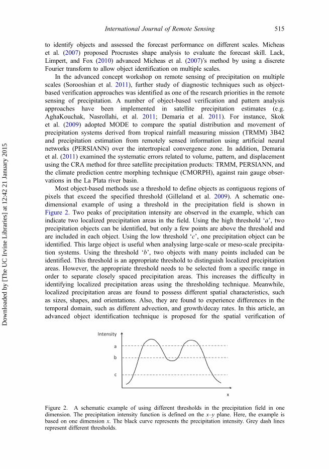
Most object-based methods use a threshold to define objects as contiguous regions ofpixels that exceed the specified threshold (Gilleland et al. 2009). A schematic one-dimensional example of using a threshold in the precipitation field is shown inFigure 2. Two peaks of precipitation intensity are observed in the example, which canindicate two localized precipitation areas in the field. Using the high threshold ‘a’, twoprecipitation objects can be identified, but only a few points are above the threshold andare included in each object. Using the low threshold ‘c’, one precipitation object can beidentified. This large object is useful when analysing large-scale or meso-scale precipita-tion systems. Using the threshold ‘b’, two objects with many points included can beidentified. This threshold is an appropriate threshold to distinguish localized precipitationareas. However, the appropriate threshold needs to be selected from a specific range inorder to separate closely spaced precipitation areas. This increases the difficulty inidentifying localized precipitation areas using the thresholding technique. Meanwhile,localized precipitation areas are found to possess different spatial characteristics, suchas sizes, shapes, and orientations. Also, they are found to experience differences in thetemporal domain, such as different advection, and growth/decay rates. In this article, anadvanced object identification technique is proposed for the spatial verification of

Intensity

a

b

c

x

Figure 2. A schematic example of using different thresholds in the precipitation field in onedimension. The precipitation intensity function is defined on the x–y plane. Here, the example isbased on one dimension x. The black curve represents the precipitation intensity. Grey dash linesrepresent different thresholds.

International Journal of Remote Sensing 515

Dow

nloa

ded

by [

The

UC

Irv

ine

Lib

rari

es]

at 1

2:42

21

Janu

ary

2015

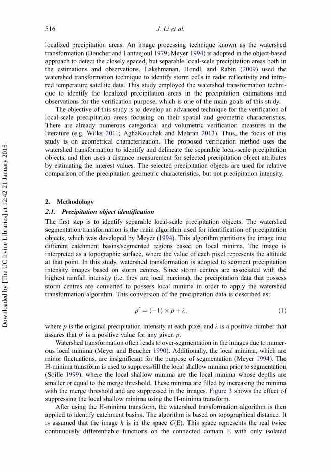
localized precipitation areas. An image processing technique known as the watershedtransformation (Beucher and Lantuejoul 1979; Meyer 1994) is adopted in the object-basedapproach to detect the closely spaced, but separable local-scale precipitation areas both inthe estimations and observations. Lakshmanan, Hondl, and Rabin (2009) used thewatershed transformation technique to identify storm cells in radar reflectivity and infra-red temperature satellite data. This study employed the watershed transformation techni-que to identify the localized precipitation areas in the precipitation estimations andobservations for the verification purpose, which is one of the main goals of this study.

The objective of this study is to develop an advanced technique for the verification oflocal-scale precipitation areas focusing on their spatial and geometric characteristics.There are already numerous categorical and volumetric verification measures in theliterature (e.g. Wilks 2011; AghaKouchak and Mehran 2013). Thus, the focus of thisstudy is on geometrical characterization. The proposed verification method uses thewatershed transformation to identify and delineate the separable local-scale precipitationobjects, and then uses a distance measurement for selected precipitation object attributesby estimating the interest values. The selected precipitation objects are used for relativecomparison of the precipitation geometric characteristics, but not precipitation intensity.

2. Methodology

2.1. Precipitation object identification

The first step is to identify separable local-scale precipitation objects. The watershedsegmentation/transformation is the main algorithm used for identification of precipitationobjects, which was developed by Meyer (1994). This algorithm partitions the image intodifferent catchment basins/segmented regions based on local minima. The image isinterpreted as a topographic surface, where the value of each pixel represents the altitudeat that point. In this study, watershed transformation is adopted to segment precipitationintensity images based on storm centres. Since storm centres are associated with thehighest rainfall intensity (i.e. they are local maxima), the precipitation data that possessstorm centres are converted to possess local minima in order to apply the watershedtransformation algorithm. This conversion of the precipitation data is described as:

p0 ¼ �1ð Þ � pþ λ; (1)

where p is the original precipitation intensity at each pixel and λ is a positive number thatassures that p′ is a positive value for any given p.

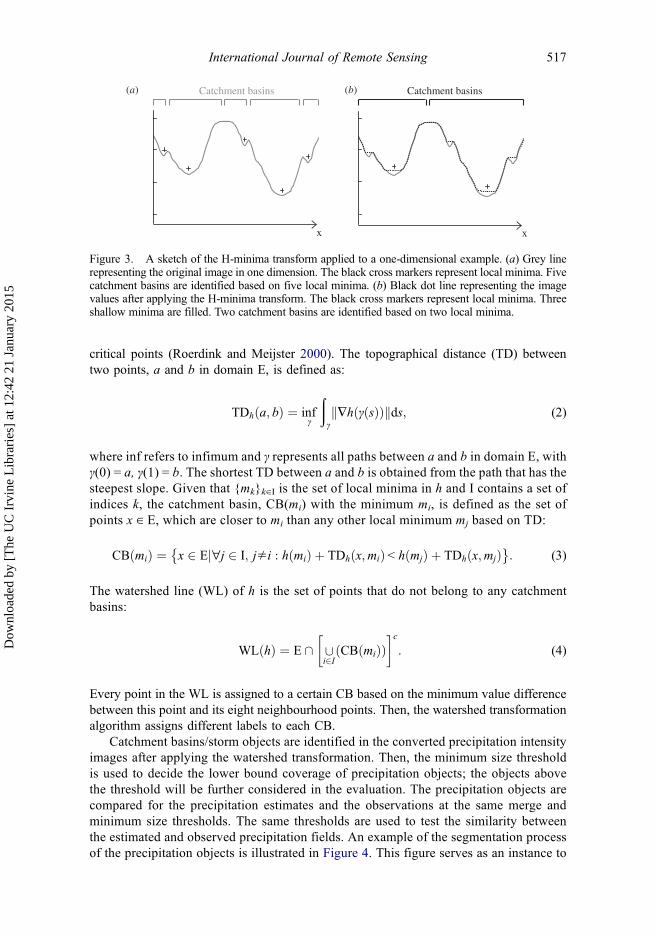
Watershed transformation often leads to over-segmentation in the images due to numer-ous local minima (Meyer and Beucher 1990). Additionally, the local minima, which areminor fluctuations, are insignificant for the purpose of segmentation (Meyer 1994). TheH-minima transform is used to suppress/fill the local shallow minima prior to segmentation(Soille 1999), where the local shallow minima are the local minima whose depths aresmaller or equal to the merge threshold. These minima are filled by increasing the minimawith the merge threshold and are suppressed in the images. Figure 3 shows the effect ofsuppressing the local shallow minima using the H-minima transform.

After using the H-minima transform, the watershed transformation algorithm is thenapplied to identify catchment basins. The algorithm is based on topographical distance. Itis assumed that the image h is in the space C(E). This space represents the real twicecontinuously differentiable functions on the connected domain E with only isolated

516 J. Li et al.

Dow

nloa

ded

by [

The

UC

Irv

ine

Lib

rari

es]

at 1

2:42

21

Janu

ary

2015

critical points (Roerdink and Meijster 2000). The topographical distance (TD) betweentwo points, a and b in domain E, is defined as:

TDhða; bÞ ¼ infγ

ðγ�hðγðsÞÞk kds; (2)

where inf refers to infimum and γ represents all paths between a and b in domain E, withγ(0) = a, γ(1) = b. The shortest TD between a and b is obtained from the path that has thesteepest slope. Given that {mk}k∈I is the set of local minima in h and I contains a set ofindices k, the catchment basin, CB(mi) with the minimum mi, is defined as the set ofpoints x ∈ E, which are closer to mi than any other local minimum mj based on TD:

CBðmiÞ ¼ x 2 Ej"j 2 I; j�i : hðmiÞ þ TDhðx;miÞ<hðmjÞ þ TDhðx;mjÞ� �

: (3)

The watershed line (WL) of h is the set of points that do not belong to any catchmentbasins:

WLðhÞ ¼ E \ [i2I

CBðmiÞð Þ� �c

: (4)

Every point in the WL is assigned to a certain CB based on the minimum value differencebetween this point and its eight neighbourhood points. Then, the watershed transformationalgorithm assigns different labels to each CB.

Catchment basins/storm objects are identified in the converted precipitation intensityimages after applying the watershed transformation. Then, the minimum size thresholdis used to decide the lower bound coverage of precipitation objects; the objects abovethe threshold will be further considered in the evaluation. The precipitation objects arecompared for the precipitation estimates and the observations at the same merge andminimum size thresholds. The same thresholds are used to test the similarity betweenthe estimated and observed precipitation fields. An example of the segmentation processof the precipitation objects is illustrated in Figure 4. This figure serves as an instance to

(a) Catchment basins Catchment basins (b)

x x

Figure 3. A sketch of the H-minima transform applied to a one-dimensional example. (a) Grey linerepresenting the original image in one dimension. The black cross markers represent local minima. Fivecatchment basins are identified based on five local minima. (b) Black dot line representing the imagevalues after applying the H-minima transform. The black cross markers represent local minima. Threeshallow minima are filled. Two catchment basins are identified based on two local minima.

International Journal of Remote Sensing 517

Dow

nloa

ded

by [

The

UC

Irv

ine

Lib

rari

es]

at 1

2:42

21

Janu

ary

2015

(a) (b)

(c) (d)

(e) (f)

(g) (h)

40N

60

50

40

30

20

10

135N

40N

35N

40N

35N

40N

35N

40N

35N

40N

35N

40N

35N

40N

35N

95W 90W 85W

Longitude

Latit

ude

Latit

ude

Latit

ude

Latit

ude

Latit

ude

Latit

ude

Latit

ude

Latit

ude

95W 90W 85W

Longitude

95W 90W 85W

Longitude

95W 90W 85W

Longitude

95W 90W 85W

Longitude

95W 90W 85W

Longitude

95W 90W 85W

Longitude

95W 90W 85W

Longitude

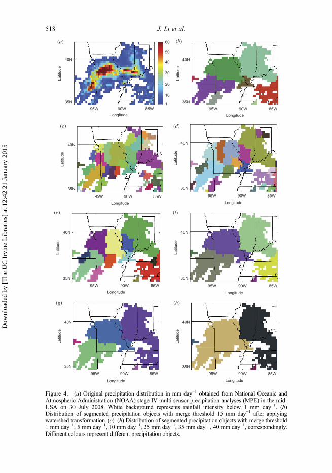
Figure 4. (a) Original precipitation distribution in mm day−1 obtained from National Oceanic andAtmospheric Administration (NOAA) stage IV multi-sensor precipitation analyses (MPE) in the mid-USA on 30 July 2008. White background represents rainfall intensity below 1 mm day−1. (b)Distribution of segmented precipitation objects with merge threshold 15 mm day−1 after applyingwatershed transformation. (c)–(h) Distribution of segmented precipitation objects with merge threshold1 mm day−1, 5 mm day−1, 10 mm day−1, 25 mm day−1, 35 mm day−1, 40 mm day−1, correspondingly.Different colours represent different precipitation objects.

518 J. Li et al.

Dow

nloa

ded

by [

The

UC

Irv

ine

Lib

rari

es]

at 1

2:42

21

Janu

ary

2015

demonstrate how the merge threshold affects the resulting precipitation objects in thereference data (i.e. observations). Here, different merge thresholds were used to showthe separation of precipitation areas. When the merge threshold is small (1 to 10 mmday−1 in this case), segmented precipitation objects tend to delineate small-scale pre-cipitation objects. On the other hand, when the merge threshold is large (greater than25 mm day−1 in this case), segmented precipitation objects tend to combine the closelyspaced precipitation areas. Therefore, the appropriate merge threshold should beselected based on the scale at which validation information is required. Note that themerge threshold can be determined based on the user’s particular application. If a user isinterested in a more detailed structure/pattern of the precipitation field, a relatively lowermerge threshold can be considered. If a user is interested in the large-scale structure/pattern of the precipitation field, a relatively higher merge threshold can be implemen-ted. In this study, a 15 mm day−1 threshold is used for a local-scale evaluation ofsatellite precipitation information.

2.2. Precipitation object evaluation

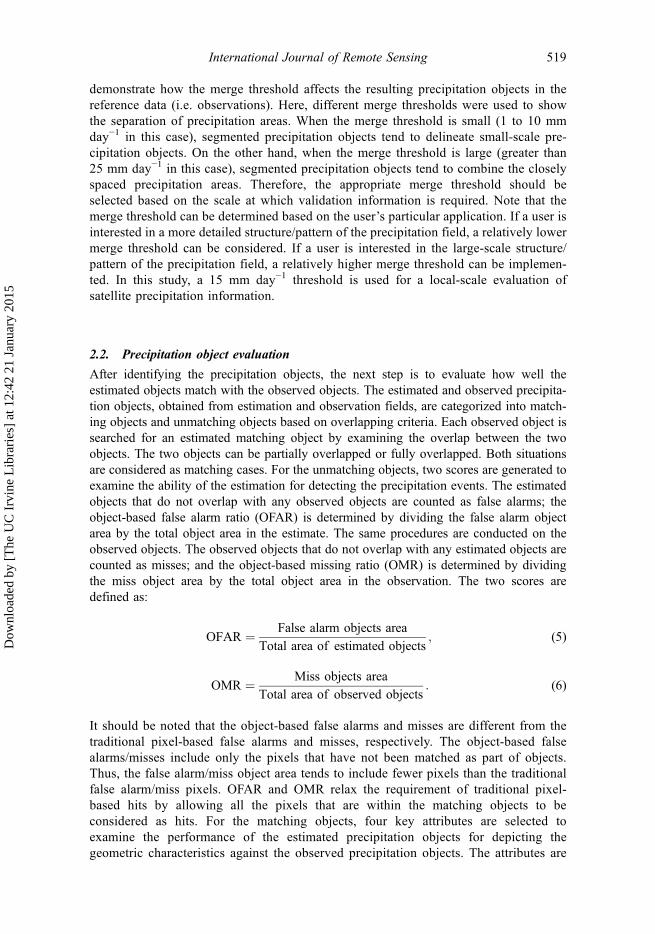
After identifying the precipitation objects, the next step is to evaluate how well theestimated objects match with the observed objects. The estimated and observed precipita-tion objects, obtained from estimation and observation fields, are categorized into match-ing objects and unmatching objects based on overlapping criteria. Each observed object issearched for an estimated matching object by examining the overlap between the twoobjects. The two objects can be partially overlapped or fully overlapped. Both situationsare considered as matching cases. For the unmatching objects, two scores are generated toexamine the ability of the estimation for detecting the precipitation events. The estimatedobjects that do not overlap with any observed objects are counted as false alarms; theobject-based false alarm ratio (OFAR) is determined by dividing the false alarm objectarea by the total object area in the estimate. The same procedures are conducted on theobserved objects. The observed objects that do not overlap with any estimated objects arecounted as misses; and the object-based missing ratio (OMR) is determined by dividingthe miss object area by the total object area in the observation. The two scores aredefined as:

OFAR ¼ False alarm objects area

Total area of estimated objects; (5)

OMR ¼ Miss objects area

Total area of observed objects: (6)

It should be noted that the object-based false alarms and misses are different from thetraditional pixel-based false alarms and misses, respectively. The object-based falsealarms/misses include only the pixels that have not been matched as part of objects.Thus, the false alarm/miss object area tends to include fewer pixels than the traditionalfalse alarm/miss pixels. OFAR and OMR relax the requirement of traditional pixel-based hits by allowing all the pixels that are within the matching objects to beconsidered as hits. For the matching objects, four key attributes are selected toexamine the performance of the estimated precipitation objects for depicting thegeometric characteristics against the observed precipitation objects. The attributes are

International Journal of Remote Sensing 519

Dow

nloa

ded

by [

The

UC

Irv

ine

Lib

rari

es]

at 1

2:42

21

Janu

ary

2015

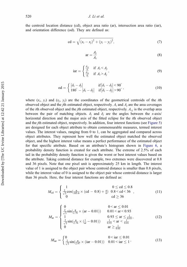
the centroid location distance (cd), object area ratio (ar), intersection area ratio (iar),and orientation difference (od). They are defined as:

cd ¼ffiffiffiffiffiffiffiffiffiffiffiffiffiffiffiffiffiffiffiffiffiffiffiffiffiffiffiffiffiffiffiffiffiffiffiffiffiffiffiffiffiffiðxi � xjÞ2 þ ðyi � yjÞ2

q; (7)

ar ¼ Aj

Ai(8)

iar ¼Ai;j

Aiif Ai <Aj

Ai;j

Ajif Ai >Aj

(; (9)

od ¼ δi � δj�� �� if δi � δj

�� ��< 90�

180� � δi � δj

�� �� if δi � δj�� ��> 90�

�; (10)

where (xi, yi) and (xj, yj) are the coordinates of the geometrical centroids of the ithobserved object and the jth estimated object, respectively. Ai and Aj are the area coveragesof the ith observed object and the jth estimated object, respectively. Ai;j is the overlap areabetween the pair of matching objects. δi and δj are the angles between the x-axis/horizontal direction and the major axis of the fitted eclipse for the ith observed objectand the jth estimated object, respectively. In addition, four interest functions (see Figure 5)are designed for each object attribute to obtain commensurable measures, termed interestvalues. The interest values, ranging from 0 to 1, can be aggregated and compared acrossobject attributes. They represent how well the estimated object matched the observedobject, and the highest interest value means a perfect performance of the estimated objectfor that specific attribute. Based on an attribute’s histogram shown in Figure 6, aprobability density function is created for each attribute. The extreme of 2.5% of eachtail in the probability density function is given the worst or best interest values based onthe attribute. Taking centroid distance for example, two extremes were discovered at 0.8and 36 pixels. Note that one pixel unit is approximately 25 km in length. The interestvalue of 1 is assigned to the object pair whose centroid distance is smaller than 0.8 pixels,while the interest value of 0 is assigned to the object pair whose centroid distance is largerthan 36 pixels. Here, the four interest functions are defined as:

Mcd ¼1 0 � cd � 0:8

2ffiffi3

p cosð π105:6 � ðcd � 0:8Þþ π

6Þ 0:8< cd< 360 cd � 36

8<: ; (11)

Mar ¼

0 0< ar � 0:012ffiffi3

p sinð π2:76 � ðar � 0:01ÞÞ 0:01< ar< 0:93

1 0:93 � ar � 10:93

2ffiffi3

p sinð π2:76 � ð1ar � 0:01ÞÞ 1

0:93 < ar < 10:01

0 ar � 10:01

8>>>>><>>>>>:

; (12)

Miar ¼0 0< iar � 0:012ffiffi3

p sinð π2:97 � ðiar � 0:01ÞÞ 0:01< iar � 1

�; (13)

520 J. Li et al.

Dow

nloa

ded

by [

The

UC

Irv

ine

Lib

rari

es]

at 1

2:42

21

Janu

ary

2015

Mod ¼1 0 � od � 1:12ffiffi3

p cosð π252:9 � ðod� 1:1Þ þ π

6Þ 1:1< od< 85:40 85:4 � od � 90

8<: : (14)

An overall interest score is generated for matching estimated/observed objects:

oi;j ¼ Mi;j;cd � wcd þMi;j;ar � war þMi;j;iar � wiar þMi;j;od � wod; (15)

oi ¼Xj2Si

ðai;j � oi;jÞ; ai;j ¼ oi;jPp2Si

oi;p; Si 2 for all jðAi;j�ϕÞ; (16)

o ¼ medianðoiÞ; (17)

where Mi,j,cd, Mi,j,ar, Mi,j,iar, and Mi,j,od are the interest values of attributes cd, ar, iar, and odbetween the ith observed and the jth estimated object pair. The terms wcd, war, wiar, andwod are the weights of each attribute, where the same weight of 25% is assigned in thisstudy. oi;j is the overall interest value of the object pair. For each observed object, aweighted interest value, oi, is obtained based on the set of matching estimated objects (Si).If the observed object matches with one estimated object, Si contains one matchingestimated object and consequently oi is equal to oi;j. If the observed object matches

1

0.8

0.6

0.4

0.2

00.8

10 20 30

36

40

Inte

rest

Val

ue

Centroid Distance/pixels

(a)

1

0.8

0.6

0.4

0.2

0

0.93 1/0.93

Inte

rest

Val

ue

0.01 1 1/0.01

Area Ratio

(b)

1

0.8

0.6

0.4

0.2

00.01

Inte

rest

Val

ue

0.2 0.4 0.6 0.8 1.0Intersection Area Ratio

(c)

1.1 85.4

30 60 90Orientation Difference/degrees

Inte

rest

Val

ue

(d)1

0.8

0.6

0.4

0.2

0

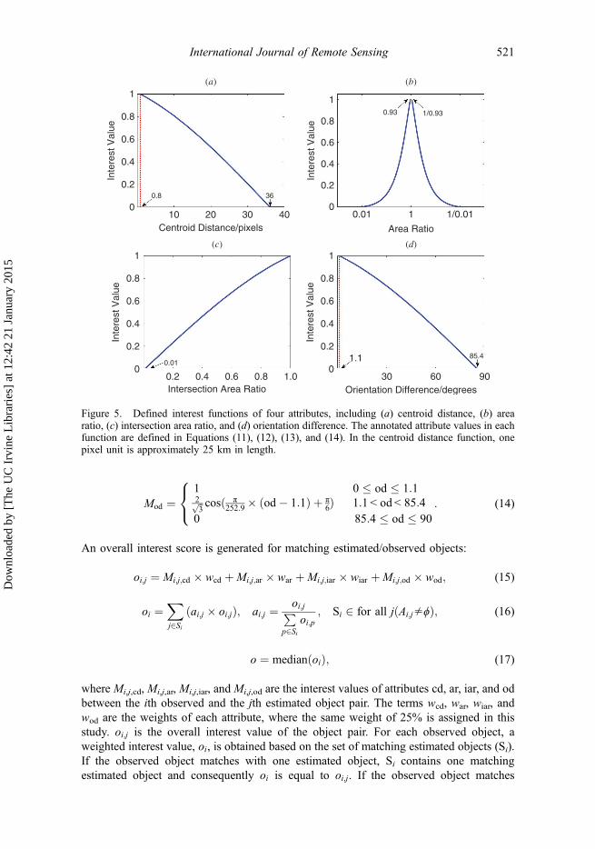
Figure 5. Defined interest functions of four attributes, including (a) centroid distance, (b) arearatio, (c) intersection area ratio, and (d) orientation difference. The annotated attribute values in eachfunction are defined in Equations (11), (12), (13), and (14). In the centroid distance function, onepixel unit is approximately 25 km in length.

International Journal of Remote Sensing 521

Dow

nloa

ded

by [

The

UC

Irv

ine

Lib

rari

es]

at 1

2:42

21

Janu

ary

2015

with multiple estimated objects, Si contains multiple matching estimated objects. oi is thencalculated using the weights ai;j, with better matches getting a higher weight. The overallinterest score, o, is the median of the weighted interest values oi from all of the matchingobserved objects. For a domain, the overall interest score, o, provides the information onthe quality of the estimated data in an aggregated sense. In general, with a small centroiddistance, a large intersection area ratio, a small object size difference, and a smallorientation difference for the matching objects, the overall interest score would be high.On the other hand, with a large centroid distance, a small intersection area ratio, a largeobject size difference, and a large orientation difference, the overall interest score wouldbe low.

3. Case study

In this section, the object-based approach described above is applied for validation of asatellite-based precipitation product against ground radar observations. It should be notedthat the case study serves as an application of the framework to examine its feasibility.

3.1. Data

The satellite-based precipitation product used in this study is PERSIANN (Hsuet al. 1997; Sorooshian et al. 2000). It is a global precipitation estimation system using

(b)1000

800

600

400

200

0403020

Area Ratio101

(d)350

250

150

50

015 30 45 60 75 90

Orientation Difference/degrees

(c)1000

0.2 0.4 0.6 0.8 1Intersection Area Ratio

800

600

400

200

0

(a)400

10 20 30 40 50Centroid Distance/pixels

300

200

100

0

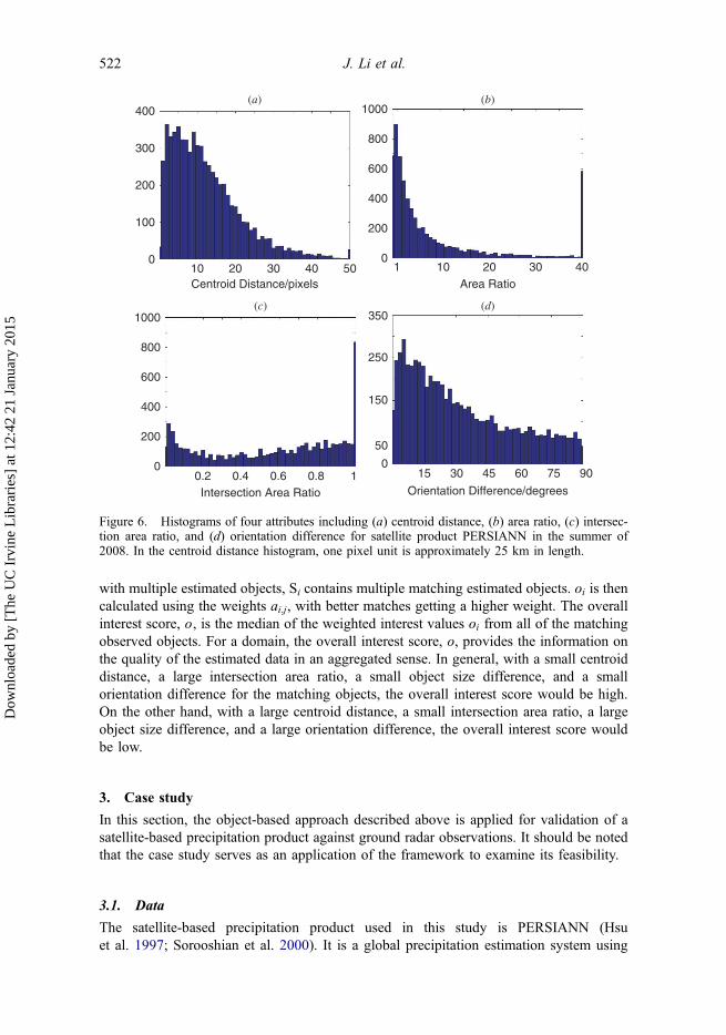
Figure 6. Histograms of four attributes including (a) centroid distance, (b) area ratio, (c) intersec-tion area ratio, and (d) orientation difference for satellite product PERSIANN in the summer of2008. In the centroid distance histogram, one pixel unit is approximately 25 km in length.

522 J. Li et al.

Dow

nloa

ded

by [

The

UC

Irv

ine

Lib

rari

es]

at 1

2:42

21

Janu

ary

2015

an artificial neural network approach. It estimates the rainfall rate at each 0.25° × 0.25°pixel based on geostationary long-wave infrared imagery and is corrected by passivemicrowave information. NOAA stage IV MPE (Lin and Mitchell 2005) is used as theground-observation reference. The stage IV data combines the precipitation measurementsfrom radar and rain gauge at a 4 km spatial resolution. Here, the stage IV data areprocessed to derive the same spatial resolution as for the PERSIANN data. Four-kilometregrid stage IV data contained in a 0.25° × 0.25° pixel are averaged to obtain the stage IVdata at a 0.25° spatial resolution. The case study is conducted at 0.25° × 0.25° on a dailyscale in the summer of 2008 over the contiguous United States (CONUS). Here, dailyprecipitation estimates are selected for evaluation, because a large number of climate andhydrologic applications require daily precipitation estimates as their inputs. In addition,the reference data obtained from ground radar and rain gauges provide good quality at the24-hour time scale. Therefore, the evaluation of precipitation estimates at the daily scale isperformed in order to provide useful information about the skill of precipitation estimatesfor the hydrology community.

3.2. Precipitation object identification

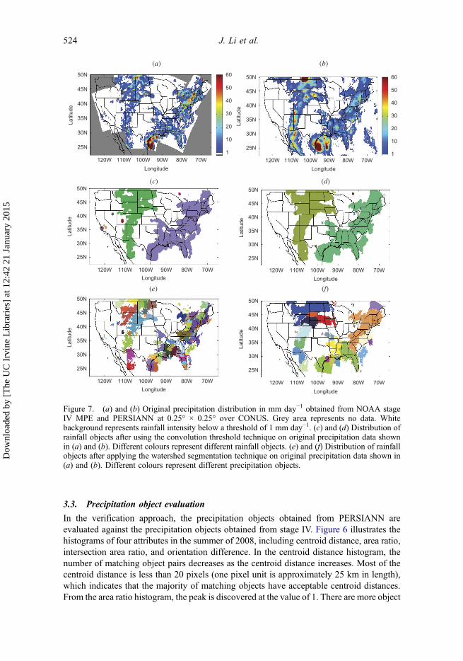
Figure 7(a) and (b) demonstrates the precipitation distribution obtained from stage IV andPERSIANN at a daily accumulation of rainfall intensity on 23 July 2008, over CONUS.Coherent areas of rainfall generated by convective storms are depicted in both figures. Ingeneral, the precipitation areas of stage IV present different spatial characteristics andstructures in the local scale compared to that of PERSIANN. Figure 7(c) and (d) showsthe precipitation objects identified using the convolution threshold technique (Daviset al. 2009). The convolution threshold technique uses the process of convolution and athreshold to identify objects in the precipitation estimation and observation. The processof convolution replaces the centred pixel value with the average over the window coveredarea. After convolution, the contiguous regions of pixels that exceed the threshold aredefined as the precipitation objects. As seen in Figure 7(c) and (d), two dominant largerainfall objects over the middle and eastern USA are observed for stage IV andPERSIANN by using this thresholding approach. These rainfall objects represent synopticscale precipitation areas and depict the precipitation structures in the synoptic scale.Figure 7(e) and (f) indicates how rainfall objects are shaped and distributed by implement-ing the watershed transformation on stage IV and PERSIANN with a merge threshold of15 mm day−1. Here, the segmented rainfall objects well represent the closely spaced, butseparable local-scale 24-hour accumulated precipitation areas for stage IV andPERSIANN. The resulting rainfall objects are the separable local-scale precipitationareas that a human expert would likely see from the precipitation fields. This demonstratesthe capability of the watershed transformation for separating the closely spaced meso-scale precipitation areas. The different precipitation objects delineate different precipita-tion areas generated from convective storms, and the precipitation object distributiondepicts the accumulated precipitation structure in the local scale. In addition,PERSIANN precipitation objects are larger in size compared to stage IV precipitationobjects. This is because PERSIANN tends to estimate larger precipitating areas as shownin Figure 7(b) compared to stage IV precipitating areas in Figure 7(a). PERSIANN usesthe cloud-top brightness temperature to estimate the precipitation that results in producinga larger coverage for precipitation systems. This implies that the watershed transformationis able to preserve the original features of the precipitation in the segmented precipitationobjects, which allows a diagnostic evaluation at the local scale.

International Journal of Remote Sensing 523

Dow

nloa

ded

by [

The

UC

Irv

ine

Lib

rari

es]

at 1

2:42

21

Janu

ary

2015

3.3. Precipitation object evaluation

In the verification approach, the precipitation objects obtained from PERSIANN areevaluated against the precipitation objects obtained from stage IV. Figure 6 illustrates thehistograms of four attributes in the summer of 2008, including centroid distance, area ratio,intersection area ratio, and orientation difference. In the centroid distance histogram, thenumber of matching object pairs decreases as the centroid distance increases. Most of thecentroid distance is less than 20 pixels (one pixel unit is approximately 25 km in length),which indicates that the majority of matching objects have acceptable centroid distances.From the area ratio histogram, the peak is discovered at the value of 1. There are more object

(a)

50N 60

50

40

30

20

10

1

45N

40N

35N

30N

25N

120W 110W 100W 90W 80W 70W

Longitude

Latit

ude

(b)

60

50

40

30

20

10

1120W 110W 100W 90W 80W 70W

Longitude

50N

45N

40N

35N

30N

25N

Latit

ude

(d)

120W 110W 100W 90W 80W 70W

Longitude

50N

45N

40N

35N

30N

25N

Latit

ude

(c)

120W 110W 100W 90W 80W 70W

Longitude

50N

45N

40N

35N

30N

25N

Latit

ude

(e)

120W 110W 100W 90W 80W 70W

Longitude

50N

45N

40N

35N

30N

25N

Latit

ude

(f)

120W 110W 100W 90W 80W 70W

Longitude

50N

45N

40N

35N

30N

25N

Latit

ude

Figure 7. (a) and (b) Original precipitation distribution in mm day−1 obtained from NOAA stageIV MPE and PERSIANN at 0.25° × 0.25° over CONUS. Grey area represents no data. Whitebackground represents rainfall intensity below a threshold of 1 mm day−1. (c) and (d) Distribution ofrainfall objects after using the convolution threshold technique on original precipitation data shownin (a) and (b). Different colours represent different rainfall objects. (e) and (f) Distribution of rainfallobjects after applying the watershed segmentation technique on original precipitation data shown in(a) and (b). Different colours represent different precipitation objects.

524 J. Li et al.

Dow

nloa

ded

by [

The

UC

Irv

ine

Lib

rari

es]

at 1

2:42

21

Janu

ary

2015

pairs with area ratios (greater than 1) than the others. This shows that PERSIANN tends togenerate larger size rain objects than stage IV. In the intersection area ratio histogram, thematching objects spread almost evenly between the lower bound and the higher bound. Apeak is noted at the value of 1, representing perfect overlapping. Finally, from the orienta-tion difference histogram, it is observed that the number of object pairs decreases as theorientation difference increases. Fifty-five per cent of the orientation difference is less than30°, which indicates that PERSIANN performs well with regard to the orientation angle.

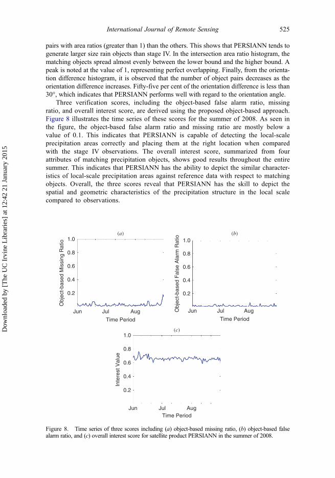
Three verification scores, including the object-based false alarm ratio, missingratio, and overall interest score, are derived using the proposed object-based approach.Figure 8 illustrates the time series of these scores for the summer of 2008. As seen inthe figure, the object-based false alarm ratio and missing ratio are mostly below avalue of 0.1. This indicates that PERSIANN is capable of detecting the local-scaleprecipitation areas correctly and placing them at the right location when comparedwith the stage IV observations. The overall interest score, summarized from fourattributes of matching precipitation objects, shows good results throughout the entiresummer. This indicates that PERSIANN has the ability to depict the similar character-istics of local-scale precipitation areas against reference data with respect to matchingobjects. Overall, the three scores reveal that PERSIANN has the skill to depict thespatial and geometric characteristics of the precipitation structure in the local scalecompared to observations.

(a)1.0

0.8

0.6

0.4

0.2

Jun Jul Aug

Time Period

Obj

ect-

base

d M

issi

ng R

atio

(b)1.0

0.8

0.6

0.4

0.2

Obj

ect-

base

d F

alse

Ala

rm R

atio

Jun Jul Aug

Time Period

(c)1.0

0.8

0.6

0.4

0.2

Inte

rest

Val

ue

Jun Jul AugTime Period

Figure 8. Time series of three scores including (a) object-based missing ratio, (b) object-based falsealarm ratio, and (c) overall interest score for satellite product PERSIANN in the summer of 2008.

International Journal of Remote Sensing 525

Dow

nloa

ded

by [

The

UC

Irv

ine

Lib

rari

es]

at 1

2:42

21

Janu

ary

2015

4. Summary and conclusions

An object-based approach is presented in this article to evaluate simulated precipitation byfocusing on separable local-scale precipitation areas. The application of the approach isdemonstrated in the validation of the satellite precipitation product PERSIANN against thestage IV rain analysis on a daily scale for the summer of 2008. The watershed transformation isadopted in the approach in order to identify the closely spaced, but separable local-scaleprecipitation areas. The application of watershed transformation allows the separation of closelyspaced precipitation areas and identification of local-scale precipitation objects in the mean-time. This assures that the precipitation object characteristics, acquired from separable local-scale precipitation areas, are diagnostic and valuable for future evaluation. In addition, the threemetrics, including the object-based false alarm ratio, missing ratio, and overall interest score, areexamined to be informative and meaningful. These three scores are capable of demonstratingwhether the simulated precipitation correctly detects the rainfall and how well the simulatedprecipitation can depict the spatial and geometric features of the precipitation structure. Hence,this object-based approach provides new insights into the object-based evaluation of precipita-tion estimation by characterizing the local-scale precipitation characteristics.

The proposed object-based approach is suggested for further implementation on othersatellite-based precipitation products. The performance for depicting the spatial and geometriccharacteristics of the precipitation structure at the local-scale can be examined for differentproducts on a daily scale. These evaluation activities using the object-based approach can beincluded in the satellite precipitation intercomparison project for a comprehensive under-standing of different satellite-based precipitation products. Another promising application ofthe approach is the assessment of NWP models. More insights can be learned from theevaluation of NWP models by focusing on the local-scale precipitation structure.

AcknowledgementsThe authors would like to acknowledge the MODE developers (Davis et al. 2009) for inspiring theresearch direction. The authors would also like to thank Yudong Tian, Christa Peters-Lidard, andPhil Arkin for their helpful suggestions. Furthermore, the authors would like to thank DanBraithwaite for his assistance with the data preparation and the reviewers for their valuablecomments and suggestions that led to the improvement of this work.

Disclosure statementNo potential conflict of interest was reported by the authors.

FundingSupport for this study was provided by the NASA NESSF fellowship [NNX10AO61H], NASAPrecipitation Measurement Mission [grant number NNX10AK07G] and US Army Research Office[grant number W911NF-11-1-0422].

ReferencesAdler, R. F., C. Kidd, G. Petty, M. Morissey, and H. M. Goodman. 2001. “Intercomparison of

Global Precipitation Products: The Third Precipitation Intercomparison Project (PIP-3).”Bulletin of the American Meteorological Society 82: 1377–1396. doi:10.1175/1520-0477(2001)082<1377:IOGPPT>2.3.CO;2.

526 J. Li et al.

Dow

nloa

ded

by [

The

UC

Irv

ine

Lib

rari

es]

at 1

2:42

21

Janu

ary

2015

AghaKouchak, A., A. Behrangi, S. Sorooshian, K. Hsu, and E. Amitai. 2011. “Evaluation ofSatellite-Retrieved Extreme Precipitation Rates across the Central United States.” Journal ofGeophysical Research 116. doi:10.1029/2010JD014741.

AghaKouchak, A., and A. Mehran. 2013. “Extended Contingency Table: Performance Metrics forSatellite Observations and Climate Model Simulations.” Water Resources Research 49: 7144–7149. doi:10.1002/wrcr.20498.

AghaKouchak, A., A. Mehran, H. Norouzi, and A. Behrangi. 2012. “Systematic and Random ErrorComponents in Satellite Precipitation Data Sets.” Geophysical Research Letters 39.doi:10.1029/2012GL051592.

AghaKouchak, A., N. Nasrollahi, J. Li, B. Imam, and S. Sorooshian. 2011. “GeometricalCharacterization of Precipitation Patterns.” Journal of Hydrometeorology 12: 274–285.doi:10.1175/2010JHM1298.1.

Ahijevych, D., E. Gilleland, B. Brown, and E. Ebert. 2009. “Application of Spatial VerificationMethods to Idealized and NWP Gridded Precipitation Forecasts.” Weather and Forecasting 24:1485–1497. doi:10.1175/2009WAF2222298.1.

Arkin, P., and J. Turk. 2006. “Program to Evaluate High Resolution Precipitation Products(PEHRPP): A Contribution to GPM Planning.” In 6th GPM International PlanningWorkshop. Annapolis, MD: NASA. Preprints.

Arkin, P. A., and P. P. Xie. 1994. “The Global Precipitation Climatology Project: First AlgorithmIntercomparison Project.” Bulletin of the American Meteorological Society 75: 401–419.doi:10.1175/1520-0477(1994)075<0401:TGPCPF>2.0.CO;2.

Baldwin, M. E., and J. S. Kain. 2006. “Sensitivity of Several Performance Measures toDisplacement Error, Bias, and Event Frequency.” Weather and Forecasting 21: 636–648.doi:10.1175/WAF933.1.

Beucher, S., and C. Lantuejoul. 1979. “Use of Watersheds in Contour Detection.” Proceedings ofInternational Workshop on Image Processing, Real-Time Edge and Motion Detection/Estimation, Rennes, September 17–21.

Casati, B., L. J. Wilson, D. B. Stephenson, P. Nurmi, A. Ghelli, M. Pocernich, U. Damrath, E. E.Ebert, B. G. Brown, and S. Mason. 2008. “Forecast Verification: Current Status and FutureDirections.” Meteorological Applications 15: 3–18. doi:10.1002/met.52.

Colle, B. A., J. B. Olson, and J. S. Tongue. 2003. “Multiseason Verification of the MM5. Part II:Evaluation of High-Resolution Precipitation Forecasts over the Northeastern United States.”Weather and Forecasting 18: 458–480. doi:10.1175/1520-0434(2003)18<458:MVOTMP>2.0.CO;2.

Davis, C. A., B. Brown, and R. Bullock. 2006a. “Object-Based Verification of PrecipitationForecasts. Part I: Methodology and Application to Mesoscale Rain Areas.” Monthly WeatherReview 134: 1772–1784. doi:10.1175/MWR3145.1.

Davis, C. A., B. Brown, and R. Bullock. 2006b. “Object-Based Verification of PrecipitationForecasts. Part II: Application to Convective Rain Systems.” Monthly Weather Review 134:1785–1795. doi:10.1175/MWR3146.1.

Davis, C. A., B. G. Brown, R. Bullock, and J. Halley-Gotway. 2009. “The Method for Object-BasedDiagnostic Evaluation (MODE) Applied to Numerical Forecasts from the 2005 NSSL/SPCSpring Program.” Weather and Forecasting 24: 1252–1267. doi:10.1175/2009WAF2222241.1.

Demaria, E. M. C., D. A. Rodriguez, E. E. Ebert, P. Salio, F. Su, and J. B. Valdes 2011. “Evaluationof Mesoscale Convective Systems in South America Using Multiple Satellite Products and anObject-Based Approach.” Journal of Geophysical Research 116. doi:10.1029/2010JD015157.

Ebert, E. E., U. Damrath, W. Wergen, and M. E. Baldwin. 2003. “The WGNE assessment of Short-term Quantitative Precipitation Forecasts.” Bulletin of the American Meteorological Society 84:481–492. doi:10.1175/BAMS-84-4-481.

Ebert, E. E., and W. A. Gallus. 2009. “Toward Better Understanding of the Contiguous Rain Area(CRA) Method for Spatial Forecast Verification.” Weather and Forecasting 24: 1401–1415.doi:10.1175/2009WAF2222252.1.

Ebert, E. E., J. E. Janowiak, and C. Kidd. 2007. “Comparison of Near-Realtime PrecipitationEstimates from Satellite Observations and Numerical Models.” Bulletin of the AmericanMeteorological Society 88: 47–64. doi:10.1175/BAMS-88-1-47.

Ebert, E. E., and J. L. McBride. 2000. “Verification of Precipitation in Weather Systems:Determination of Systematic Errors.” Journal of Hydrology 239: 179–202. doi:10.1016/S0022-1694(00)00343-7.

International Journal of Remote Sensing 527

Dow

nloa

ded

by [

The

UC

Irv

ine

Lib

rari

es]

at 1

2:42

21

Janu

ary

2015

Faurès, J.-M., D. C. Goodrich, D. A. Woolhiser, and S. Sorooshian. 1995. “Impact of Small-ScaleSpatial Rainfall Variability on Runoff Modeling.” Journal of Hydrology 173: 309–326.doi:10.1016/0022-1694(95)02704-S.

Foufoula-Georgiou, E., and V. Vuruputur. 2001. “Patterns and Organization in Precipitation.” InSpatial Patterns in Catchment Hydrology: Observations and Modeling, edited by R. Graysonand G. Blöschl, 82–104. Cambridge: Cambridge University Press.

Gilleland, E., D. Ahijevych, B. G. Brown, B. Casati, and E. E. Ebert. 2009. “Intercomparison ofSpatial Forecast Verification Methods.” Weather and Forecasting 24: 1416–1430. doi:10.1175/2009WAF2222269.1.

Gilleland, E., D. Ahijevych, B. G. Brown, and E. E. Ebert. 2010. “Verifying Forecasts Spatially.”Bulletin of the American Meteorological Society 91: 1365–1373. doi:10.1175/2010BAMS2819.1.

Goodrich, D., J. Faures, D. Woolhiser, L. Lane, and S. Sorooshian. 1995. “Measurement andAnalysis of Small-Scale Convective Storm Rainfall Variability.” Journal of Hydrology 173:283–308. doi:10.1016/0022-1694(95)02703-R.

Hsu, K., X. Gao, S. Sorooshian, and H. V. Gupta. 1997. “Precipitation Estimation from RemotelySensed Information Using Artificial Neural Networks.” Journal of Applied Meteorology 36:1176–1190. doi:10.1175/1520-0450(1997)036<1176:PEFRSI>2.0.CO;2.

Lack, S., G. L. Limpert, and N. I. Fox. 2010. “An Object-Oriented Multiscale Verification Scheme.”Weather and Forecasting 25: 79–92. doi:10.1175/2009WAF2222245.1.

Lakshmanan, V., K. Hondl, and R. Rabin. 2009. “An Efficient, General-Purpose Technique forIdentifying Storm Cells in Geospatial Images.” Journal of Atmospheric and OceanicTechnology 26: 523–537. doi:10.1175/2008JTECHA1153.1.

Lin, Y., and K. E. Mitchell. 2005. “The NCEP Stage II/IV Hourly Precipitation Analyses:Development and Applications.” In 19th Conference on Hydrology. San Diego, CA:American Meteor Society 1.2. Preprints.

Marzban, C., and S. Sandgathe. 2006. “Cluster Analysis for Verification of Precipitation Fields.”Weather and Forecasting 21: 824–838. doi:10.1175/WAF948.1.

Marzban, C., and S. Sandgathe. 2008. “Cluster Analysis for Object-Oriented Verification of Fields:A Variation.” Monthly Weather Review 136: 1013–1025. doi:10.1175/2007MWR1994.1.

Mass, C. F., D. Ovens, K. Westrick, and B. A. Colle. 2002. “Does Increasing Horizontal ResolutionProduce More Skillful Forecasts?” Bulletin of the American Meteorological Society 83:407–430. doi:10.1175/1520-0477(2002)083<0407:DIHRPM>2.3.CO;2.

McBride, J. L., and E. E. Ebert. 2000. “Verification of Quantitative Precipitation Forecasts fromOperational Numerical Weather Prediction Models over Australia.” Weather and Forecasting15: 103–121. doi:10.1175/1520-0434(2000)015<0103:VOQPFF>2.0.CO;2.

Mehran, A., and A. AghaKouchak. 2014. “Capabilities of Satellite Precipitation datasets to EstimateHeavy Precipitation Rates at Different Temporal Accumulations.” Hydrological Processes 28:2262–2270. doi:10.1002/hyp.9779.

Meyer, F. 1994. “Topographic Distance and Watershed Lines.” Signal Processing 38: 113–125.doi:10.1016/0165-1684(94)90060-4.

Meyer, F., and S. Beucher. 1990. “Morphological Segmentation.” Journal of Visual Communicationand Image representation 1: 21–46. doi:10.1016/1047-3203(90)90014-M.

Micheas, A. C., N. I. Fox, S. A. Lack, and C. K. Wikle. 2007. “Cell Identification and Verificationof QPF Ensembles Using Shape Analysis Techniques.” Journal of Hydrology 343: 105–116.doi:10.1016/j.jhydrol.2007.05.036.

Olson, D. A., N. W. Junker, and B. Korty. 1995. “Evaluation of 33 Years of QuantitativePrecipitation Forecasting at the NMC.” Weather and Forecasting 10: 498–511. doi:10.1175/1520-0434(1995)010<0498:EOYOQP>2.0.CO;2.

Roerdink, J. B. T. M., and A. Meijster. 2000. “The Watershed Transform: Definitions, Algorithmsand Parallelization Strategies.” Fundamenta Informaticae 41: 187–228.

Sapiano, M. R. P., and P. A. Arkin. 2009. “An Intercomparison and Validation of High-ResolutionSatellite Precipitation Estimates with 3-Hourly Gauge Data.” Journal of Hydrometeorology 10:149–166. doi:10.1175/2008JHM1052.1.

Skok, G., J. Tribbia, J. Rakovec, and B. Brown. 2009. “Object-Based Analysis of Satellite-DerivedPrecipitation Systems over the Low- and Midlatitude Pacific Ocean.” Monthly Weather Review137: 3196–3218. doi:10.1175/2009MWR2900.1.

528 J. Li et al.

Dow

nloa

ded

by [

The

UC

Irv

ine

Lib

rari

es]

at 1

2:42

21

Janu

ary

2015

Smith, E. A., J. E. Lamm, R. Adler, J. Alishouse, K. Aonashi, E. Barrett, P. Bauer, W. Berg, A.Chang, R. Ferraro, J. Ferriday, S. Goodman, N. Grody, C. Kidd, K. Kniveton, C. Kummerow,G. Liu, F. Marzano, A. Mugnai, W. Olsen, G. Petty, A. Shibata, R. Spencer, F. Wentz, T.Wilheit, and E. Zipser. 1998. “Results of WetNet PIP-2 Project.” Journal of the AtmosphericSciences 55: 1483–1536. doi:10.1175/1520-0469(1998)055<1483:ROWPP>2.0.CO;2.

Soille, P. 1999. Morphological Image Analysis: Principles and Applications, 170–171. New York:Springer-Verlag.

Sorooshian, S., A. AghaKouchak, P. Arkin, J. Eylander, E. Foufoula-Georgiou, R. Harmon,J. Hendrickx, B. Imam, R. Kuligowski, B. Skahill, and G. Skofronick-Jackson. 2011.“Advanced Concepts on Remote Sensing of Precipitation at Multiple Scales.” Bulletin of theAmerican Meteorological Society 92: 1353–1357. doi:10.1175/2011BAMS3158.1.

Sorooshian, S., K.-L. Hsu, X. Gao, H. V. Gupta, B. Imam, and D. Braithwaite. 2000. “Evaluation ofPERSIANN System Satellite-Based Estimates of Tropical Rainfall.” Bulletin of the AmericanMeteorological Society 81: 2035–2046. doi:10.1175/1520-0477(2000)081<2035:EOPSSE>2.3.CO;2.

Tian, Y., C. D. Peters-Lidard, J. B. Eylander, R. J. Joyce, G. J. Huffman, R. F. Adler, K. Hsu, F. J.Turk, M. Garcia, and J. Zeng 2009. “Component Analysis of Errors in Satellite-BasedPrecipitation Estimates.” Journal of Geophysical Research 114. doi:10.1029/2009JD011949.

Wernli, H., C. Hofmann, and M. Zimmer. 2009. “Spatial Forecast Verification MethodsIntercomparison Project: Application of the SAL Technique.” Weather and Forecasting 24:1472–1484. doi:10.1175/2009WAF2222271.1.

Wernli, H., M. Paulat, M. Hagen, and C. Frei. 2008. “SAL—A Novel Quality Measure for theVerification of Quantitative Precipitation Forecasts.” Monthly Weather Review 136: 4470–4487.doi:10.1175/2008MWR2415.1.

Wilks, D. S. 2011. Statistical Methods in the Atmospheric Sciences. Amsterdam: Academic.

International Journal of Remote Sensing 529

Dow

nloa

ded

by [

The

UC

Irv

ine

Lib

rari

es]

at 1

2:42

21

Janu

ary

2015