it I \ if

LIBRARIES

V *&nft^S^Off®*

Digitized by the Internet Archive

in 2011 with funding from

Boston Library Consortium Member Libraries

http://www.archive.org/details/mcmcapproachtoclOOcher

0/HB31.M415

Massachusetts Institute of Technology

Department of Economics

Working Paper Series

AN MCMC APPROACH TO CLASSICAL ESTIMATION

Victor Chernozhukov

Han Hong

Working Paper 03-21

December 2002

Room E52-251

50 Memorial Drive

Cambridge, MA 02142

This paper can be downloaded without charge from the

Social Science Research Network Paper Collection at

http://ssrn.com/abstract=42037

1

MASSACHUSETTS INSTITUTEOF TECHNOLOGY

SEP 1 9 2003

LIBRARIES

An MCMC Approach to Classical Estimation

Victor Chernozhukova, Han Hong6

° Department of Economics, Massachusetts Institute of Technology, Cambridge, MA 02142, USAb Department of Economics, Princeton University, Princeton, NJ 08544, USA

First Version: October 2000 This Version: December 2002 1

Project Funded by the National Science Foundation.

Abstract

This paper studies computationally and theoretically attractive estimators referred here as to the Laplace

type estimators (LTE). The LTE include means and quantiles of Quasi-posterior distributions defined as

transformations of general (non-likelihood-based) statistical criterion functions, such as those in GMM,nonlinear IV, empirical likelihood, and minimum distance methods. The approach generates an alternative

to classical extremum estimation and also falls outside the parametric Bayesian approach. For example,

it offers a new attractive estimation method for such important semi-parametric problems as censored and

instrumental quantile regression, nonlinear IV, GMM, and value-at-risk models. The LTE's are computed

using Markov Chain Monte Carlo methods, which help circumvent the computational curse of dimensionality.

A large sample theory is obtained and illustrated for regular cases.

JEL Classification: C10, Cll, C13, C15

Keywords: Laplace, Bayes, Markov Chain Monte Carlo, GMM, instrumental regression, censored

quantile regression, instrumental quantile regression, empirical likelihood, value-at-risk

1 Introduction

A variety of important econometric problems pose not only a theoretical but a serious computational

challenge, cf. Andrews (1997). A small (and by no means exhaustive) set of such examples include (1)

Powell's censored median regression for linear and nonlinear problems, (2) nonlinear rV estimation,

e.g in the Berry et al. (1995) model, (3) the instrumental quantile regression, (4) the continuous-

updating GMM estimator of Hansen et al. (1996), and related empirical likelihood problems. These

problems represent a formidable practical challenge as the extremum estimators are known to be

difficult to compute due to highly nonconvex criterion functions with many local optima (but well

pronounced global optimum). Despite extensive efforts, see notably Andrews (1997), the problem

of extremum computation remains a formidable impediment in these applications.

'A shorter version of this paper is forthcoming in Journal of Econometrics 115 (August 2003), p. 293-346

This paper develops a class of estimators, which we call the Laplace type estimators (LTE) or

Quasi-Bayesian estimators (QBE),2 which are defined similarly to Bayesian estimators but use gen-

eral statistical criterion functions in place of the parametric likelihood function. This formulation

circumvents the curse of dimensionality inherent in the computation of the classical extremum esti-

mators by instead focusing on LTE which are functions of integral transformations of the criterion

functions and can be computed using Markov Chain Monte Carlo methods (MCMC), a class of simu-

lation techniques from Bayesian statistics. This formulation will be shown to yield both computable

and theoretically attractive new estimators to such important problems as (l)-(4) listed above. Al-

though the aforementioned applications are mostly microeconometric, the obtained results extend

to many other models, including GMM and quasi-likelihoods in the nonlinear dynamic framework

of Gallant and White (1988).

The class of LTE's or QBE's aim to explore the use of the Laplace approximation (developed by

Laplace to study large sample approximations of Bayesian estimators and for use in other non-

statistical problems) outside of the canonical Bayesian framework - that is, outside of parametric

likelihood settings when the likelihood function is not known. Instead, the approach relies upon

other statistical criterion functions of interest in place of the likelihood, transforms them into proper

distributions - Quasi-posteriors - over a parameter of interest, and defines various moments and

quantiles of that distribution as the point estimates and confidence intervals, respectively. It is

important to emphasize that the underlying criterion functions are mainly motivated by the analogy

principle in place of the likelihood principle, are not the likelihoods (densities) of the data, and are

most often semi-parametric. 3

The resulting estimators and inference procedures possess a number of good theoretical and com-

putational properties and yield new, alternative approaches for the important problems mentioned

earlier. The estimates are as efficient as the extremum estimates; and, in many cases, the inference

procedures based on the quantiles of the Quasi-posterior distribution or other posterior quantities

yield asymptotically valid confidence intervals, which also perform notably well in finite samples.

For example, in the quantile regression setting, those intervals provide valid large sample and excel-

lent small sample inference without requiring nonparametric estimation of the conditional density

function (needed in the standard approach). The obtained results are general and useful - they cover

the examples listed above under general, non-likelihood based conditions that allow discontinuous,

non-smooth semi-parametric criterion functions, and data generating processes that range from iid

settings to the nonlinear dynamic framework of Gallant and White (1988). The results thus extend

the theoretical work on large sample theory of Bayesian procedures in econometrics and statistics,

e.g. Bickel and Yahav (1969), Ibragimov and Has'minskii (1981), Andrews (1994b), Kim (1998).

The LTE's are computed using MCMC, which simulates a series of parameter draws such that

2A preferred terminology is taken here to be the 'Laplace Type Estimators', since the term 'Quasi-Bayesian

Estimators' is already used to name Bayesian procedures that use either 'vague' or 'data-dependent' prior or multiple

priors, cf. Berger (2002).3 In this paper, the term 'semi-parametric' refers to the cases where the parameters of interest are finite-dimensional

but there are nonparametric nuisance parameters such as unspecified distributions.

the marginal distribution of the series is (approximately) the Quasi-posterior distribution of the

parameters. The estimator is therefore a function of this series, and may be given explicitly as the

mean or a quantile of the series, or implicitly as the minimizer of a smooth globally convex function.

As stated above, the LTE approach is motivated by the estimation and inference efficiency as well as

computational attractiveness. Indeed, the LTE approach is as efficient as the extremum approach,

but generally may not suffer from the computational curse of dimensionality (through the use of

MCMC). The reason is that the computation of LTE's is itself statistically motivated. LTE's are

typically means or quantiles of a quasi-posterior distribution, hence can be estimated (computed)

at the parametric rate l/\/B, where B is the number of draws from that distribution (functional

evaluations). In contrast, the mode (extremum estimator) is estimated (computed) by the MCMCand similar grid-based algorithms at the nonparametric rate (l/B) d+?p

, where d is the parameter

dimension and p is the smoothness order of the objective function.

Another useful feature of LT estimation is that, by using information about the overall shape of the

objective function, point estimates and confidence intervals may be calculated simultaneously. It

also allows incorporation of prior information, and allows for a simple imposition of constraints in

the estimation procedure.

The remainder of the paper proceeds as follows. Section 2 formally defines and further motivates the

Laplace type estimators with several examples, reviews the literature, and explains other connections.

The motivating examples, which are all semi-parametric and involve no parametric likelihoods, will

justify the pursuit of a more general theory than is currently available. Section 3 develops the large

sample theory, and Sections 3 and 4 further explore it within the context of the econometric examples

mentioned earlier. Section 4 briefly reviews important computational aspects and illustrates the use

of the estimator through simulation examples. Section 5 contains a brief empirical example, and

Section 6 concludes.

Notation. Standard notation is used throughout. Given probability measure P, —

>

p denotes

the convergence in (outer) probability with respect to the outer probability P*; —>£ denotes the

convergence in distribution under P*, etc. See e.g. van der Vaart and Wellner (1996) for definitions.

\x\ denotes the Euclidean norm y/x'x; B$(x) denotes the ball of radius <5 centered at x. A notation

table is given in the appendix.

2 Laplacian or Quasi-Bayesian Estimation: Definition and Motivation

2.1 Motivation

Extremum estimators are usually motivated by the analogy principle and defined as maximizers

of random average-like criterion functions Ln ((?), where n denotes the sample size. n_1 Ln (6) are

typically viewed as transformations of sample averages that converge to criterion functions M (9) that

are maximized uniquely at some 9q. Extremum estimators are usually consistent and asymptotically

normal, cf. Amemiya (1985), Gallant and White (1988), Newey and McFadden (1994), Potscher

and Prucha (1997). However, in many important cases, actually computing the extremum estimates

remains a large problem, as discussed by Andrews (1997).

Example 1: Censored and Nonlinear Quantile Regression. A prominent model in economet-

rics is the censored median regression model of Powell (1984). Powell's censored quantile regression

estimator is defined to maximize the following nonlinear objective function

n

Ln W = - X) w« ' PriXi - q{Xi,e)), q{Xi,9) = max (0,g(Xu 9)),

where pT (u) = (r — l(u < 0)) u is the check function of Koenker and Bassett (1978), w, is a weight,

and Y{ is either positive or zero. Its conditional quantile q(Xi,9) is specified as max(0,g(Xi,8)). The

censored quantile regression model was first formulated by Powell (1984) as a way to provide valid

inference in Tobin-Amemiya models without distributional assumptions and with heteroscedasticity

of unknown form. The extremum estimator based on the Powell's criterion function, while theoret-

ically elegant, has a well-known computational difficulty. The objective function is similar to that

plotted in Figure 1 - it is nonsmooth and highly nonconvex, with numerous local optima, posing a

formidable obstacle to the practical use of this extremum estimator; see Buchinsky and Hahn (1998),

Buchinsky (1991), Fitzenberger (1997), and Khan and Powell (2001) for related discussions. In this

paper, we shall explore the use of LT estimators based on Powell's criterion function and show that

this alternative is attractive both theoretically and computationally.

Example 2: Nonlinear IV and GMM. Amemiya (1977), Hansen (1982), Hansen et al. (1996)

introduced nonlinear IV and GMM estimators that maximize

where m; (9) is a moment function defined such that the economic parameter of interest solves

Em,i{9 ) = 0.

The weighting matrix may be given by Wn {9) — [jj Y^?-i m « (#) m « W J+ °p0) or other sensible

choices. Note that the term "op (l)" in Ln implicitly incorporates generalized empirical likelihood

estimators, which will be discussed in section 4. Up to the first order, objective functions of empirical

likelihood estimators for 9 (with the Lagrange multiplier concentrated out) locally coincide with L„.

Applications of these estimators are numerous and important (e.g. Berry et al. (1995), Hansen et al.

(1996), Imbens (1997)), but while global maxima are typically well-defined, it is also typical to see

many local optima in applications. This leads to serious difficulties with applying the extremum

approach in applications where the parameter dimension is high. As in the previous example, LTE's

provide a computable and theoretically attractive alternative to extremum estimators. Furthermore,

Quasi-posterior quantiles provide a valid and effective way to construct confidence intervals and

explore the shape of the objective function.

Example 3: Instrumental and Robust Quantile Regression. Instrumental quantile regression

may be defined by maximizing a standard nonlinear IV or GMM objective function4

where

mi ((?) = (r - l(Yi < q(Dh Xi,9)) Zu

Yi is the dependent variable, Dt- is a vector of possibly endogeneous variables, Xi is a vector of

regressors, Z\ is a vector of instruments, and Wn (9) is a positive definite weighting matrix, e.g.

W„{9) lYimi (9)mi (9)' +op (l) or Wn (tf) = _i__ -j^^Z't

Tt i I J. T ) /6i=l J v ' L i=l

or other sensible versions. Motivations for estimating equations of this sort arise from traditional

separable simultaneous equations, cf. Amemiya (1985), and also more general nonseparable simul-

taneous equation models and heterogeneous treatment effect models.5

Clearly, a variety of Huber (1973) type robust estimators can be defined in this way. For example,

suppose in the absence of endogeneity

q{X,9) = X'l3(T),

then Z = f(X) can be constructed to preclude the influence of outliers in X on the inference. For

example, choosing Z\j = \{X{j < Xj), j — 1, ..., dim(X), where Xj denotes the median of {X{j, i < n}

produces an approach that is similar in spirit to the maximal regression depth estimator of Rousseeuw

and Hubert (1999), whose computational difficulty is well known, as discussed in van Aelst et al.

(2002). The resulting objective function in (/3) is highly robust to both outliers in Xij and Y,. In

fact, it appears that the breakdown properties of this objective function are similar to those of the

objective function of Rousseeuw and Hubert (1999).

Despite a clear appeal, the computational problem is daunting. The function Ln is highly non-

convex, almost everywhere flat, and has numerous discontinuities and local optima.6 (Note that the

global optimum is well pronounced.) Figure 1 illustrates the situation. Again, in this case the LTEapproach will yield a computable and theoretically attractive alternative to the extremum-based

estimation and inference.7 Furthermore, we will show that the Quasi-posterior confidence intervals

provide a valid and effective way to construct confidence intervals for parameters and their smooth

4 Early variants based on the Wald instruments go back to Mood (1950) and Hogg (1975), cf. Koenker (1998).5 See Chernozhukov and Hansen (2001) for the development of this direction.6Macurdy and Timmins (2001) propose to smooth out the edges using kernels, however this does not eliminate

non-convexities and local optima; see also Abadie (1995).TAnother computationally attractive approach, based on an extension of Koenker and Bassett (1978) quantile

regression estimator to instrumental problems like these, is given in Chernozhukov and Hansen(2001).

functions without non-parametric estimation of the conditional density function evaluated at quan-

tiles (needed in standard approach).

The LTE's studied in this paper can be easily computed through Markov Chain Monte Carlo and

other posterior simulation methods. To describe these estimators, note that although the objective

function Ln (9) is generally not a log-likelihood function, the transformation

e >Wtt(0)

is a proper distribution density over the parameter of interest, called here the Quasi-posterior. Here

k (9) is a weight or prior probability density that is strictly positive and continuous over ©, for

example, it can be constant over the parameter space. Note that p„ is generally not a true posterior

in the Bayesian sense, since it may not involve the conditional data density or likelihood, and is thus

generally created through non-Bayesian statistical learning.

The Quasi-posterior mean is then defined as

e = JeePn{e)de = f&

e(^ZlU * ™

where is the parameter space. Other quantities such as medians and quantiles will also be

considered. A formal definition of LTE's is given in Definition 1.

In order to compute these estimators, using Markov Chain Monte Carlo methods, we can draw a

Markov chain (see Figure 1),

S={9^,9^,.. .,0<D>),

whose marginal density is approximately given by p„(9), the Quasi-posterior distribution. Then the

estimate 9, e.g. the Quasi-posterior mean, is computed as

1B

B2=1

Analogously, for a given continuously differentiable function g : -¥ M, the 90%-confidence intervals

are constructed simply by taking the .05-th and .95-th quantiles of the sequence

9(S) = (g(e^),...,g(9W)),

see Figure 1. Under the information equality restrictions discussed later, such confidence regions are

asymptotically valid. Under other conditions, it is possible to use other Quasi-posterior quantities

such as the variance-covariance matrix of the series S to define asymptotically valid confidence

regions, see Section 3. It shall be emphasized repeatedly that the validity of this approach does not

depend on the likelihood formulation.

2.2 Formal Definitions

Let pn (u) be a penalty or loss function associated with making an incorrect decision. Examples of

pn (u) include

i. p„ (u) = iT/nu]2

, the squared loss function,

ii. pn (u) = y/n^2j=1 \iij\, the absolute deviation loss function,

iii. p„ (u) = y/n^j_1(tj — 1 (uj < 0)) Uj, for Tj € (0, 1) for each j, the check loss function of

Koenker and Bassett (1978).

The parameter is assumed to belong to the subset of Euclidean space. Using the Quasi-posterior

pn density in (2.1), define the Quasi-posterior risk function as:

On (0 = /e pAO - C) Pn ffl* = fe*V- (j^Zl^de )»• (2 -3)

Definition 1 The class of LTE minimize the function Qn {0 ?n (%-3) for various choices of pn :

e = arginf [Qn (C)]. (2.4)

The estimator 9 is a decision rule that is least unfavorable given the statistical (non-likelihood)

information provided by the probability measure pn , using the loss function pn - In particular, the

loss function pn may asymmetrically penalize deviations from the truth, and 7r may give differential

weights to different values of 9. The solutions to the problem (2.4) for loss functions i-iii include

the Quasi-posterior means, medians, and marginal Tj-th. quantiles, respectively. 8

2.3 Related Literature

Our analysis will rely heavily on the previous work on Bayesian estimators in the likelihood setting.

The initial large sample work on Bayesian estimators was done by Laplace (see Stigler (1975) for a

detailed review). Further early work of Bernstein (1917) and von Mises (1931) has been considerably

extended in both econometric and statistical research, cf. Ibragimov and Has'minskii (1981), Bickel

and Yahav (1969), Andrews (1994b), Phillips and Ploberger (1996), and Kim (1998), among others.

In general, Bayesian asymptotics require very delicate control of the tail of the posterior distribution

and were developed in useful generality much later than the asymptotics of extremum estimators.

The treatments of Bickel and Yahav (1969) and Ibragimov and Has'minskii (1981) are most useful

for the present setting, but are inevitably tied down to the likelihood setting. For example, the

8This formulation implies that conditional on the data, the decision 8 satisfies Savage's axioms of choice under

uncertainty with subjective probabilities given by p„ (these include the usual asymmetry and negative transitivity of

strict preference relationship, independence, and some other standard axioms).

latter treatment relies heavily on Hellinger bounds that are firmly rooted in the objective function

being a likelihood of iid data. However, the general flavor of the approach is suited for the present

purposes. The treatment of Bickel and Yahav (1969) can be easily extended to smooth, possibly

incorrect iid likelihoods,9 but does not apply to censored median regression or any of the GMM type

settings. Andrews (1994b) and Phillips and Ploberger (1996) study the large sample approximation

of posteriors- and posterior odds ratio tests in relation to the classical Wald tests in the context

of smooth, correctly specified likelihoods. Kim (1998) derives the limit behavior of posteriors in

likelihood models over shrinking neighborhood systems. Kim's approach and related approaches

have been important in describing the essence of posterior behavior, but the limit behavior of point

estimates like ours does not follow from it.10

Formally and substantively, none of the above treatments apply to our motivating examples and the

estimators given in Definition 1. These examples do not involve likelihoods, deal mostly with GMMtype objective functions, and often involve discontinuous and non-smooth criterion functions to which

the above mentioned results do not apply. In order to develop the theory of LTE's for such examples,

we extend the previous arguments. The results obtained here enable the use of Bayesian tools outside

of the Bayesian framework - covering models with non-likelihood-based criterion functions, such as

examples listed earlier and other semi-parametric objective functions that may, for example, depend

on preliminary estimates of infinite-dimensional nuisance parameters. Moreover, our results apply to

general forms of data generating processes - from the cross-sectional framework of Amemiya (1985)

to the nonlinear dynamic framework of Gallant and White (1988) and Potscher and Prucha (1997).

Our motivating problems are all semi-parametric, and there are several pure Bayesian approaches

to such problems, see notably Doksum and Lo (1990), Diaconis and Freedman (1986), Hahn (1997),

Chamberlain and Imbens (1997), Kottas and Gelfand (2001). Semi-parametric models have some

parametric and nonparametric components, e.g. the unspecified nonparametric distribution of data

in Examples 1-3. The mentioned papers proceed with the pure Bayesian approach to such problems,

which involves Bayesian learning about these two components via a two-step process. In the first step,

Bayesian non-parametric learning with Dirichlet priors is used to form beliefs about the joint non-

parametric density of data, and then draws of the non-parametric density ("Bayesian bootstrap") are

made repeatedly to compute the extremum parameter of interest. This approach is purely Bayesian,

as it fully conforms to the Bayes learning model. It is clear that this approach is generally quite

different from LTE's or QBE's studied in this paper, and in applications, it still requires numerous

re-computations of the extremum estimates in order to construct the posterior distribution over the

parameter of interest. In sharp contrast, the LT estimation takes a "shortcut" by essentially using

the common criterion functions as posteriors, and thus entirely avoids both the estimation of the

nonparametric distribution of the data and the repeated computation of extremum estimates.

9See Bunke and Milhaud (1998) for an extension to the more than three times differentiable smooth misspecified

iid likelihood case. The conditions do not apply to GMM or even Example 1.

I0 E.g. to describe the behavior of posterior median one needs to know f* pn {6)d9 which requires the study of

Ln (&) beyond the compact \.f\/n neighborhoods of &o- Similarly, the posterior mean is J^°00 9pn (8)dd, which also

requires the study of the complete Ln (6).

Finally note that the LTE approach has a limited-information or semi-parametric nature in the

sense that we do not know or are not willing to specify the complete data density. The limited-

information principle is powerfully elaborated in the recent work of Zellner (1998), who starts with

a set of moment conditions, calculates the maximum entropy densities consistent with the moment

equations, and uses those as formal (misspecified) likelihoods. While in the present framework,

calculation of the maximum entropy densities is not needed, the large sample theory obtained here

does cover Zellner's (1998) estimators as one fundamental case. Related work by Kim (2002) derives

a limited information likelihood interpretation for certain smooth GMM settings. 11 In addition,

the LTE's based on the empirical likelihood are introduced in Section 4 and motivated there as

respecting the limited information principle.

3 Large Sample Properties

This section shows that under general regularity conditions the Quasi-posterior distribution con-

centrates at the speed T./\/n around the true parameter 9 as measured by the "total variation of

moments" norm (and total variation norm as a special case), that the LT estimators are consistent

and asymptotically normal, and that Quasi-posterior quantiles and other relevant quantities provide

asymptotically valid confidence intervals.

3.1 Assumptions

We begin by stating the main assumptions. In addition, it is assumed without further notice that

the criterion functions Ln {8) and other primitive objects have the standard measurability properties.

For example, given the underlying probability space (ft, T,P), for any w € ft, Ln (9) is a measurable

function of 9, and for any 9 € 0, Ln (9) is a random variable, that is a measurable function of w.

ASSUMPTION 1 (Parameter) The true parameter 9 belongs to the interior of a compact con-

vex subset of Euclidean space Rd.

ASSUMPTION 2 (Penalty Function) The loss function pn : Rd -> M+ satisfies:

i. p„(u) — p(y/nu), where p(u) > and p(u) — iff u — 0,

ii. p is convex and p(h) < 1 4- \h\p for some p > 1,

Hi. <p(£) = JRi p(u — f)e-u' a"du is minimized uniquely at some £* € Kd

for any finite a > 0,

iv. the weighting function n : —> R+ is a continuous, uniformly positive density function.

"Kim (2002) also provided some useful asymptotic results for exp(L n (0)) using the shrinking neighborhood ap-

proach. However, Kim's (2002) approach does not cover the estimators and procedures considered here, see previous

footnote.

ASSUMPTION 3 (Identifiability) For any <5 > 0, there exists e > 0, such that

D, j sup -(Ln (0)-Ln (6o))<-e\

[\e-9 \>6n\ 1J

ASSUMPTION 4 (Expansion) For 9 in an open neighborhood of 0o>

i. Ln (9) - Ln (ft,) = (9 - e )' A„ (6> ) - \{9 - 0o)' [nJn (0O )] (9 - 9 ) + Rn (9),

ii. n-^(9 )An (9 ) /y/E -m tf(0,I),

Hi. Jn (9o) — 0(1) and fln (9o) = 0(1) are uniformly in n positive-definite constant matrices,

iv. for each e > there is a sufficiently small 5 > and large M > such that

(a) limsupP*! sup Jg" <g ' > el < e,

f&; limsupP*] sup |-RnW| >e > = 0.

3.2 Discussion of Assumptions

In the following we discuss the stated assumptions under which Theorem 1-4 stated below will be

true. We argue that these assumptions are simple but encompass a wide variety of econometric

models - from cross-sectional models to nonlinear dynamic models. This means that Theorems 1-4

are of wide interest and applicability.

In general, Assumptions 1-4 are related to but different from those in Bickel and Yahav (1969) and

Ibragimov and Has'minskii (1981). The most substantial differences appear in Assumption 4, and are

due to the general non-likelihood setting. Also in Assumption 4 we introduce Huber type conditions

to handle the tail behavior of discontinuous and non-smooth criterion functions. In general, the

early approaches are inevitably tied to the iid likelihood formulation, which is not suited for the

present purposes.

The compactness Assumption 1 is conventional. It is shown in the proof of Theorem 1 that it is not

difficult to drop compactness. For example, in the case of Quasi-posterior quantiles in Theorem 3,

it is only required that 7r is a proper density; in the case of Quasi-posterior variances in Theorem 4,

it is only required that Je \9\2n(9)d9 < oo; and for the general loss functions considered in Theorem

2 it is required that Je \0\pir(0)d9 < oo. Of course, compactness guarantees all of the above given

Assumption 2. Also, that the parameter is on the interior of the parameter space rules out some

non-regular cases; see for example Andrews (1999).

Assumption 2 imposes convexity on the penalty function. We do not consider non-convex penalty

functions for pragmatic reasons. One of the main motivations of this paper is the generic com-

putability of the estimates, given that they solve well-defined convex optimization problems. The

10

domination condition, p(h) < 1 + \h\p for some 1 < p < oo, is conventional and is satisfied in all

examples of p we gave.

The assumption that (p(£) = / p(u — £)e~*''"'du oc Ep(Af(0, o_1

) — £) attains a unique minimum at

some finite f* for any positive definite o is required, and it clearly holds for all of examples of p we

mentioned. In fact, when p is symmetric, £* = by Anderson (1955)'s lemma.

Assumption 3 is implied by the usual uniform convergence and unique identification conditions as

in Amemiya (1985). The proof of Lemma 1 can be found in Amemiya (1985) and White (1994).

LEMMA 1 Given Assumption 1, Assumption 3 holds if there is a function Mn {9) that

i. is nonstochastic, continuous on Q, for any S > 0, limsupn (supi 9_ 9i

><sMn (9) — Mn (6 )) < 0,

it. Ln (8) jn — Mn (6) converges to zero in (outer) probability uniformly over Q.

Assumption 4 is satisfied under the conditions of Lemma 2, which are known to be mild in nonlinear

models. Assumption 4.ii requires asymptotic normality to hold, and is generally a weak assumption

for cross-sectional and many time-series applications. Assumption 4.iii rules out the cases of mixed

asymptotic normality for some non-stationary time series models (which can be incorporated at a

notational cost with different scaling rates).

Assumption 4.iv easily holds when there is enough smoothness.

LEMMA 2 Given Assumptions 1 and 3, Assumption 4 holds with

A n (0o ) = V 9L„(0o ) and Jn (8 ) = -V99>Mn (9 ) = 0(1), if

i. for some 6 > 0, Ln (9) and Mn (6) are twice continuously differentiable in 6 when \6 — 6q\ < 6,

ii. there is fln {9 ) such that n- 1/2{9 )VeLn {8 )/s/h~ -^ A/"(0,7), J„(0O ) = 0(1) and Qn (9 )

=

0(1) are uniformly positive definite, and

Hi. for some 6 > and each e >

limsupP*] sup \Vee'Ln {9)/n-Vee'Mn (9)\>e'{ sup \Vge>Ln (9)/n-Vee'Mn (e)\>e\=0.[\e-9 \<6

J

Lemma 2 is immediate, hence its proof is omitted. Both Lemmas 1 and 2 are simple but useful

conditions that can be easily verified using standard uniform laws of large numbers and central limit

theorems. In particular, they have been proven to hold for criterion functions corresponding to

1. Most smooth cross-sectional models described in Amemiya (1985);

11

2. The smooth nonlinear stationary and dynamic GMM and Quasi-likelihood models of Hansen

(1982), Gallant and White (1988) and Potscher and Prucha (1997), covering Gordin(mixingale

type) conditions and near-epoch dependent processes such as ARMA, GARCH, ARCH, and

other models alike;

3. General empirical likelihood models for smooth moment equation models studied by Imbens

(1997), Kitamuraand Stutzer (1997), Newey and Smith (2001), Owen (1989,1990,1991, 2001),

Qin and Lawless (1994), and the recent extensions to the conditional moment equations.

Hence the main results of this paper, Theorems 1-4, apply to these fundamental econometric and

statistical models. Moreover, Assumption 4 does not require differentiability of the criterion function

and thus holds even more generally. Assumption 4.iv is a Huber-like stochastic equicontinuity

condition, which requires that the remainder term of the expansion can be controlled in a particular

way over a neighborhood of 6q. In addition to Lemma 2, many sufficient conditions for Assumption

4 are given in empirical process literature, e.g. Amemiya (1985), Andrews (1994a), Newey (1991),

Pakes and Pollard (1989), and van der Vaart and Wellner (1996). Section 4 verifies Assumption 4

for the leading models with nonsmooth criterion functions, including the examples discussed in the

previous section.

3.3 Convergence in the Total Variation of Moments Norm

Under Assumptions 1-4, we show that the Quasi-posterior density concentrates around #o at the

speed 1/y/n as measured by the total variation of moments norm, and then use this preliminary

result to prove all other main results.

Define the local parameter h as a normalized deviation from 9q and centered at the normalized

random "score function"

:

h = y/n~ (9 - 0„) - Jn (Bo)'1 A„ (9 ) lyfc.

Define by the Jacobi rule the localized Quasi-posterior density for h as

p'n (h) = -)=pn (hl^fc + 9 + Jn (Oo)-

1 An (0O ) /»)

Define the total variation of moments norm for a real-valued measurable function / on S as

\\f\\TVMM =J

(l+\h\a)\f(h)\dh.

THEOREM 1 ( Convergence in Total Variation of Moments Norm) Under Assumptions

1 - 4, for any < a < 00,

\\PnW ~ Plo(h)\\TVMM = f (1 + \h\a

)\P*

n (h)- P

*

x (h)\dh^p 0,

12

where Hn = {y/n{9 - 9 )- Jn (0O )

-1 An (0O ) /y/K : 9 e 0} and

Theorem 1 shows that pn (9) is concentrated at a l/y/n neighborhood of 9 as measured by the total

variation of moments norm. For large n, pn (9) is approximately a random normal density with the

random mean parameter 9q + Jn (0o)_

A„ (9a) /n, and constant variance parameter Jn (^o)_1

/n -

Theorem 1 applies to general statistical criterion functions Ln (9), hence it covers the parametric

likelihood setting as a fundamental case, in particular implying the Bernstein-Von Mises theorems,

which state the convergence of the likelihood posterior to the limit random density in the total

variation norm. Note also that the total variation norm results from setting a — in the total

variation of moments norm. The use of the latter is needed to deduce the convergence of LTE's such

as the posterior means or variances in Theorems 2-4.

3.4 Limit Results for Point Estimates and Confidence Intervals

As a consequence of Theorem 1, Theorem 2 establishes y/n- consistency and asymptotic normality

of LTE's. When the loss function p (•) is symmetric, LTE's are asymptotically equivalent to the

extremum estimators.

Recall that the extremum estimator y/n(9ex — 9q), where 9ex = argsup9ee Ln (9), is first order-

equivalent to

Un =^Jn (9 )- 1An (9 ).

y/n

Given that the p* approaches p*^, it may be expected that the LTE y/n{9 - 9q) is asymptotically

equivalent to

Zn - arg inf I / p(z- u)p1 (it - Un ) du \ .

z£® dI JR* J

To see a relationship between Zn and Un , define

6„ c« > - ars inL i / p(z - u)p~ (") du\ >

which exists by Assumption 2.12

If p is symmetric, i.e. p(h) — p(—h), then by Anderson's lemma

6„(»o> = °- Hence

Zn — £j„(s )"*" ^">

and we are prepared to state the result.

12 For example, in the scalar parameter case, if p(h) = (a — l(h < 0))/i, the constant £j(s ) = qa Jn{9o)'' 2

, where

qa is the Q-quantile of Af{0, 1).

13

THEOREM 2 (LTE in Large Samples) Under Assumptions 1-4,

y/ii0 - 0b) = 6.(.o) + Vn + Op (l), n;^ 2(0o)J„(eo)f/n->i JV(0 ,/).

Hence

// ioss function pn is symmetric, i.e. pn (h) = pn (—h) for all h, £j„(» )= for each n.

In order for the Quasi-posterior distribution to provide valid large sample confidence intervals, the

density ofWn = J\f (0, Jn{9a)^Un {9o)Jn{9o)~^) should coincide with that ofp^ (h). This requires

I hh'pl(h)dh = Jn (9 )- 1 ~ Var(W„) ee Jn(0 )-*n„{9o)Jn(9o)-\

or equivalently

^rt(^o) ~ Jn(8o),

which is a generalized information equality. The information equality is known to hold for

regular, correctly specified likelihoods. It is also known to hold for appropriately constructed criterion

functions of generalized method of moments, minimum distance estimators, generalized empirical

likelihood estimators, and properly weighted extremum estimators; see Section 4.

Consider construction of the confidence intervals for the quantity g{9 ), and suppose g is continuously

differentiable. Define

Fg,n(x)= / pn {9)d9, and c9 ,„(a) — inf{i : Fti„{x) > a}.Jeee:g(9)<x

Then a LT confidence interval is given by [cgt

„(a/2),cgjn (l — a/2)] . As previously mentioned, these

confidence intervals can be constructed by using the a/2 and 1 — a/2 quantiles of the MCMCsequence

(g(9^),...,g(9^))

and thus are quite simple in practice. In order for the intervals to be valid in large samples, one needs

to ensure the generalized information equality, which can be done easily through the use of optimal

weighting in GMM and minimum-distance criterion functions or the use of generalized empirical

likelihood functions; see Section 4.

Consider now the usual asymptotic intervals based on the A- method and any estimator with the

property

y/n~{9-0) = J„(B )- 1 ^„(9)/y/K+op (l).

Such intervals are usually given by

where qa is the a-quantile of the standard normal distribution. The following theorem establishes

the large sample correspondence of the Quasi-posterior confidence intervals to the above intervals.

14

THEOREM 3 (Large Sample Inference I) Suppose Assumptions 1-4 hold. In addition sup-

pose that the generalized information equality holds:

lim Jn {9 )Qn {9 )- 1 =1.n—nx>

Then for any a €E (0, 1)

cg ,n (a) - g{9) - qa

y/^^''-w-2inm = 0p(*\

,

and

lim P*{c9,„(a/2) < g(9 ) < c9,„(l - a/2)) = 1 -a.7i—yoo I J

One practical limitation of this result arises in the case of regression criterion functions (M-estimators),

where achieving the information equality may require nonparametric estimation of appropriate

weights, e.g. as in censored quantile regression discussed in Section 4. This may entirely be avoided

by using a different method for construction of confidence intervals. Instead of the Quasi-posterior

quantiles, we can use the Quasi-posterior variance as an estimate of the inverse of the population

Hessian matrix J~ 1

(9o), and combine it with any available estimate of Qn {9o) (which typically is

easier to obtain) in order to obtain the A-method style intervals. The usefulness of this methods is

particularly evident in the censored quantile regression, where direct estimation of Jn (9o) requires

use of nonparametric methods.

THEOREM 4 (Large Sample Inference II) Suppose Assumptions 1-4 hold. Define for =

fe 9pn (e)de,

J-\9 ) = f n(9- 9)(9 - 9)'pn (9)d6,Je

and

c9in (a)= g{9) + qa

\/v^(^ , ^( flo)-'^(«oV-(°°)-'^^W)

where nn ((9 )n- 1(6> )^p /. Then JTl {9 )Jn (9 )- 1^p I, and

lim Wc9 ,n (a/2) < g(9 ) < c9 ,n (l - a/2)) = 1 - a.

In practice Jn (#o)-1

is computed by multiplying by n the variance-covariance matrix of the MCMCsequence S= (9^,9^,...,

9

<-B1).

4 Applications to Selected Problems

This section further elaborates the approach through several examples. Assumptions 1-4 cover a wide

variety of smooth econometric models (by virtue of Lemma 1 and Lemma 2). Thus, what follows

next is mainly motivated by models with non-smooth moment equations, such as those occurring

in Examples 1-3. Verification of the key Assumption 4 is not immediate in these examples, and

Propositions 1-3 and the forthcoming examples show how to do this in a class of models that are of

prime interest to us.

15

4.1 Generalized Method of Moments and Nonlinear Instrumental Variables

Going back to Example 2, recall that a typical model that underlies the applications of GMM is a

set of population moment equations:

Emi(6)=Q if and only if 9 = 9 . (4.1)

Method of moment estimators involve maximizing an objective function of the form

Ln (9) = -n(gn (9))'Wn (9)(gn (9))/2, (4.2)

9n(0) = -Vm,(ff), (4.3)n *—

'

Wn (0) = W{9) + op (1) uniformly in e 0, (4.4)

W (9) > and continuous uniformly in 9 (E 0, (4.5)

W(9 ) = flim Varh/^flo)]!-1

• (4.6)

The choice (4.6) of the weighting matrix implies the generalized information equality under standard

regularity conditions.

Generally, by a Central Limit Theorem \/™<?n(#o)->d f̂ '{0,W'~ 1

(9o)), so that the objective function

can be interpreted as the approximate log-likelihood for the sample moments of the data gn {ff)- Thus

we can think of GMM as an approach that specifies an approximate likelihood for selected moments

of the data without specifying the likelihood of the entire data. 13

We may impose Assumptions 1-4 directly on the GMM objective function. However, to highlight

the plausibility and elaborate on some examples that satisfy Assumption 4 consider the following

proposition.

Proposition 1 (Method-of-Moments and Nonlinear IV) Suppose that Assumptions 1-2 hold,

and that for all 9 in 0, m,-(0) is stationary and ergodic, and

i. conditions (4-l)-(4-5) hold,

ii. J{9) = G{9)'W{9)G(9) > and is continuous, G{9) = V gEmi{9) is continuous,

Hi. An (9 )/^= -Vn~gn(e yW(9 )G(9 )^d A'(O,n(0o )), Q(9 ) =G(9 )'W(9 )G(9Q ),

iv. for any e > 0, there is 6 > such that

limsuppJ sup^^W-^))-(^W-^(y))l >e l <e . (4.7,

r^co \\e-B'\<s l + y/ri\9-e'\J

Then Assumption 4 holds. In addition the information equality holds by construction. Therefore the

conclusions of Theorems 1-4 hold with An (# ), ftn (9o) = fi (#o) and Jn {9 )= J (9q) defined above,

where the condition (4- 6) is only needed for the conclusions of Theorem 3 to hold.

13This does not help much in terms of providing formal asymptotic results for the GMM model.

16

Therefore, for symmetric loss functions pni the LTE is asymptotically equivalent to the GMMextremum estimator. Furthermore, the generalized information equality holds by construction, hence

Quasi-posterior quantiles provide a computationally attractive method of "inverting" the objective

function for the confidence intervals.

For twice continuously differentiable smooth moment conditions, the smoothness conditions on

V$Ln (9) and Vee'Ln {9) stated in Lemma 2 trivially imply condition iv in Proposition 1. More

generally, Andrews (1994a), Pakes and Pollard (1989) and van der Vaart and Wellner (1996) provide

many methods to verify that condition in a wide variety of method-of-moments models.

Example 3 Continued. Instrumental median regression falls outside of both the classical Bayesian

approach and the classical smooth nonlinear IV approach of Amemiya (1977). Yet the conditions of

Proposition 1 are satisfied under mild conditions:

i. (Yi,Di,Xi 7 Zi) is an iid data sequence, E[m.i(9o)Zi] = 0, and 9q is identifiable,

ii. {m,i(9) = (r - 1(Y; < q{Di,Xi,9))) Zu 9 € 0} is a Donsker class,14 Esupg |m;(0)|

2 < oo,

iii. G{9) = VeErmie) = -EfYlDiX ,z {q{D,X,9))ZVeq{D,X,9)' is continuous,

iv. J{9) = G{9)'W(9)G{9) > and is continuous in an open ball at 9 .

\tmn .

In this case the weighting matrix can be taken as

Wn (9) = —?—r(l-r)

so that the information equality holds. Indeed, in this case

n(0o ) = G(9 )'W(9 )G(9 ) = J(9 ),

where

W(9 ) = plim Wn (9 ) = [Var m^n)]-1

, Var mi {9 ) = r(l - T)EZiZ[.

When the model q is linear and the dimension of D is small, there are computable and practical

estimators in the literature. 15 In more general models, the extremum estimates are quite difficult to

compute, and the inference faces the well-known difficulty of estimating sparsity parameters.

On the other hand, the Quasi-posterior median and quantiles are easy to compute and provide

asymptotically valid confidence intervals. Note that the inference does not require the estimation of

14This is a very weak restriction on the function class, and is known to hold for all practically relevant functional

forms, see van der Vaart (1999).I5These include e.g. the "inverse" quantile regression approach in Chernozhukov and Hansen (2001), which is an

extension of Koenker and Bassett (1978)'s quantile regression to endogenous settings.

17

the density function. The simulation example given in Section 5 strongly supports this alternative

approach.

Another important example which poses computational challenge is the estimation problem of Berry

et al. (1995). This example is similar in nature to the instrumental quantile regression, and the

application of the LT methods may be fruitful there.

4.2 Generalized Empirical Likelihood

A class of objective functions that are first-order equivalent to optimally weighted GMM (after

recentering) can be formulated using the generalized empirical likelihood framework.

A class of generalized empirical likelihood functions(GEL) are studied in Imbens et al. (1998), Kita-

mura and Stutzer (1997), and Newey and Smith (2001). For a set of moment equations Em^do) =that satisfy the conditions of section 4.1, define

n

Ln (0, 7 ) = J2 (a (m, (0)'7) - a (0))

.

(4.8)

Then set

where 7(0) solves

and p = dim(mj).

£„(*) = £„ (0,7W), (4-9)

7(0)=arg inf^.LB(0,7), (4.10)

The scalar function s(-) is a strictly convex, finite, and three times differentiable function on an open

interval of R containing 0, denoted V, and is equal to +00 outside such an interval, s () is normalized

so that both Vs (0) = 1 and V2s (0) = 1. The choices of the function s(w) = — ln(l — v), exp(u), and

(1 +v) 2/2 lead to the well-known empirical likelihood, exponential tilting, and continuous-updating

GMM criterion functions.

Simple and practical sufficient conditions for Lemma 2 are given in Qin and Lawless (1994), Imbens

et al. (1998), Kitamura (1997), Kitamura and Stutzer (1997), including stationary weakly dependent

data, Newey and Smith (2001), and Christoffersen et al. (1999). Thus, the application of LTE's to

these problems is immediate.

To illustrate a further use of LTE's we state a set of simple conditions geared towards non-smooth

microeconometric applications such as the instrumental quantile regression problem. These regu-

larity conditions imply the first order equivalence of the GEL and GMM objective functions. The

Donskerness condition below is a weak assumption that is known to hold for all reasonable linear

and nonlinear functional forms encountered in practice, as discussed in van der Vaart (1999).

Proposition 2 (Empirical likelihood Problems) Suppose that Assumptions 1- 2 hold, and that

the following conditions are satisfied: for some S > and all €

18

i. condition (4-1) holds and that m{(9) is iid,

ii. dP[mi{9) < x]/d6 is continuous in 9 uniformly in x : \x\ < K, for K in iii.

Hi. supi e_g i <s |m,-(0)| < K a.s., for some constant K

iv. {m{(9),9 € 0} is Donsker class, where

Vn~9n(0o) = 4= f>i W^^(0/W), V (9 ) = E{mi{0o)mi{0o y} > 0,

then Assumptions 3 and 4 hold, and thus the conclusions of Theorems 1-4 are true with

A„ (ftO/Vn = yft9n(0 )V.(J&o)-*G(9 )->d JV(O,n(0o )),

n($ )=G(9 yV(9 )- i G(9 ),

J(9 ) = G(9 )'V(9 r 1G(9o), G(0 ) = VeEmi {9 ).

The information equality holds in this case.

Another (equivalent) way to proceed is through the dual formulation. Consider the following criterion

function

n n n

Ln (9) = sup Y^ft(7rj) subject to Y^m;((?)7Tj = 0, y^7r; = 1, (4.11)jri,...,ir„e[0,l] i=1 i=1 i=1

where h is the Cressie-Reid divergence criterion, cf. Newey and Smith (2001)

1 (l?^1 - 1

h(*)7(7 + 1)

The function Ln (9) in (4.11) is the generalized empirical likelihood function for 9 with the con-

centrated out probabilities. In fact, (4.11) corresponds to (4.9) by the argument given in Qin and

Lawless (1994) p.303-304, so that Proposition 2 covers (4.11) as a special case up to renormalization.

Empirical probabilities 7?;(0)'s are obtained in (4.11) using the extremum method. The case 7= —

1

yields the empirical likelihood case, where 7fi(9)'s are obtained through the maximum likelihood

method. Taking 7 = yields the exponential tilting case, where 7r,(#)'s are obtained through

minimization of the Kullback-Leibler distance from the empirical distribution. Taking 7 = 1 yields

the continuous-updating case, where 7?j(#)'s are obtained through the minimization of the Euclidean

distance from the empirical distribution. Each approach generates the implied probabilities T?i{9)

given 9. Qin and Lawless (1994) and Newey and Smith (2001) provide the formulas:

n

S?iW = Vs(7(ff),m i(0))/X> S (7Wm I-(0)).

19

The Quasi-posterior for 9 and 7r,(0) can be used for predictive inference. Suppose m,i(0) = m(Xi,9)

for some random vector Xj. Then the Quasi-posterior predictive probability is given by

P{Xi eA} = JY^miiXi € A]pn {9)dB = Jhn (9)pn [0)dB,

=hn (9)

which can be computed by averaging over the MCMC sequence evaluated at hn ,(hn (9^), ..., hn(9^))

It follows similarly to the proof of Theorem 1 in Qin and Lawless (1994) that y/n(P{Xi e A} —

P{Xi € A})->d JV(0,n„) , where n„ = P{X{ 6 A}(1 - P{X{ € A}) - Emi(9o)'l{Xi € A} UEmi(9 )l{Xi eA},U = V(9o)~

1 {I ~ G(^)J{0o)- 1 G(9o)V(9o)-1}.

4.3 M-estimation

M-estimators, which include many linear and nonlinear regressions as special cases, typically maxi-

mize objective functions of the form

n

Ln {9) =Yjm i {e).

i=l

rtii (9) need not be the log likelihood function of observation i, and may depend on preliminary

non-parametric estimation. Assumptions 1-3 usually are satisfied by uniform laws of large numbers

and by unique identification of the parameter; see for example Amemiya (1985) and Newey and

McFadden (1994). The next proposition gives a simple set of sufficient conditions for Assumption 4.

Proposition 3 (M-problems) Suppose Assumptions 1-3 hold for the criterion function specified

above with the following additional conditions: Uniformly in 9 in an open neighborhood of 9q, rrii{9)

is stationary and ergodic, and for fnn (9) = Yl7=i "i,-(0)/n,

i. there exists m,(9o) such that Erhi(9o) — for each i and, for some 5 > 0,

m.i{9) - mi{9 ) - m;(0o )'(0 - 9 )> is a, : \9 — 0q\ < 6> is a Donsker class,

\9-9\

E[mn {9) - mn (9 )- mn (0o)'(O - 9 )]

2 = o{\9 - O |

2),

n

ii. J(9) — — Vee'E[m,i{9)] is continuous and nonsingular in a ball at 9q.

Then Assumption 4 holds. Therefore, the conclusions of Theorems 1, 2, and 4 hold. If in addition

J{9o) = fi(# ), then the conclusions of Theorem 3 also hold.

20

The above conditions apply to many well known examples such as LAD, see for example van der Vaart

and Wellner (1996). Therefore, for many nonlinear regressions, Quasi-posterior means, modes, and

medians are asymptotically equivalent, and Quasi-posterior quantiles provide asymptotically valid

confidence statements if the generalized information equality holds. When the information equality

fails to hold, the method of Theorem 4 provides valid confidence intervals.

Example 1 Continued. Under the conditions given in Powell (1984) or Newey and Powell (1990)

for the censored quantile regression, the assumptions of Proposition 3 are satisfied. Furthermore, it

is not difficult to show that when the weights ui* are nonparametrically estimated, the conditions of

Newey and Powell (1990) imply Assumption 4. Under iid sampling, the use of efficient weighting

"> = RT^r) *' <412

)

where /, = fYi \Xi(qi), Qi — q{Xi;6a), validates the generalized information equality, and the Quasi-

posterior quantiles form asymptotically valid confidence intervals. Indeed, since

J(*°> =T{\- T )

E^VqiV^ fOT Vqi = 9?(Xi ' 9o)/d6 > (4J3

)

and

with

we have

1 1n

-=An (0o ) =TV»r (T- \{Yi < qi))Vqi -„ jV(0, n(0o )), (4.14)*Jn •Jn -f—

'v v t=i

n{9o) = 7o^)^V9iV^' (415)

n(flo) = A0 ). (4.16)

For this class of problems, the Quasi-posterior means and medians are asymptotically equivalent

to the extremum estimators. The Quasi-posterior quantiles provide asymptotically valid confidence

intervals when the efficient weights are used. However, estimation of efficient weights requires prelim-

inary estimation of parameter 9 . When other weights are used, the method of Theorem 4 provides

valid confidence intervals.

5 Computation and Simulation Examples

In this section we briefly discuss the MCMC method and present simulation examples.

5.1 Markov Chain Monte Carlo

The Quasi-posterior density is proportional to

Pn {e)<xeL^ 6\{e).

21

In most cases we can easily compute eL"^Tr{9). However, computation of the point estimates and

confidence intervals typically requires evaluation of integrals like

Je g(9)e^eM0)M

Je eL~Wir(9)d0{

'

for various functions g. For problems for which no analytic solution exists for (5.1), especially in

high dimensions, MCMC methods provide powerful tools for evaluating integrals like the one above.

See for example Chib (2001), Geweke and Keane (2001), and Robert and Casella (1999) for excellent

treatments.

MCMC is a collection of methods that produce an ergodic Markov chain with the stationary distri-

bution pn . Given a starting value 0(°' , a chain (#(') , 1 < t < B) is generated using a transition kernel

with stationary distribution pn , which ensures the convergence of the marginal distribution of 9^top,,. For sufficiently large B, the MCMC methods produce a dependent sample (9^

a\9^1\...,9^)

whose empirical distribution approaches pn . The ergodicity and construction of the chains usually

imply that as B -> oo,

1B

r

o£s(0(°Hi> / 9W)Pn(8)d9.

We stress that this technique does not rely on the likelihood principle and can be fruitfully used for

computation of LTE's. (Appendix B provides the formal details.)

One of the most important MCMC methods is the Metropolis-Hastings algorithm.

Metropolis-Hastings (MH) algorithm with Quasi-Posteriors. Given the Quasi-posterior

density pn {9) oc eLn<

-6\{9), known up to a constant, and a prespecified conditional density q{9'\9),

generate (9^°\ ..., 9(B) ) in the following way,

1. Choose a starting value 9^.

2. Generate £ from g(0w) |?)-

3. Update 6^'+1 > from 9^ for j = 1, 2, ..., using

£ with probability p(#(i) ,07+1) _ 10W> with probability l-p{9^,0 '

where

Note that the most important quantity in the algorithm is the probability p(x, y) of the move from

an "old" point x to the "new" point y, which depends on how much of an improvement in e Ln ^n{y)

a possible "new" value of y yields relative to eLn ^Tx{x) at the "old" value x. Thus, the generated

22

chain of draws spends a relatively high proportion of time in the higher density regions and a lower

proportion in the lower density regions. Because such proportions of times are balanced in the right

way, the generated sequence of parameter draws has the requisite marginal distribution, which we

then use for computation of means, medians, and quantiles. (How closely the sequence travels near

the mode is not relevant.)

Another important choice is the transition kernel q, also called the instrumental density. It turns

out that a wide variety of kernels yield Markov chains that converge to the distribution of interest.

One canonical implementation of the MH algorithm is to take

Q{x\y) =f{\x-y\),

where / is a density symmetric around 0, such as the Gaussian or the Cauchy density. This implies

that the chain (9^) is a random walk. This is the implementation we used in this paper. Chib

(2001), Geweke and Keane (2001) and Robert and Casella (1999) can be consulted for important

details concerning the implementation and convergence monitoring of the algorithm.

It is now worth repeating that the main motivation behind the LTE approach is based on its

efficiency properties (stated in sections 3 and 4) as well as computational attractiveness. Indeed,

the LTE approach is as efficient as the extremum approach, but may avoid the computational curse

of dimensionality through the use of MCMC. LTE's are typically means or quantiles of a Quasi-

posterior distribution, hence can be computed (estimated) at the parametric rate 1/y/B, 16 where Bis the number of MCMC draws (functional evaluations). Indeed, under canonical implementations,

the MCMC chains are geometrically mixing, so the rates of convergence are the same as under

independent sampling. In contrast, the extremum estimator (mode) is computed (estimated) by

the MCMC and similar grid-based algorithms at the nonparametric rate (l/B) d+?p, where d is the

parameter dimension and p is the smoothness order of the objective function.

We used an optimistic tone regarding the performance of MCMC. Indeed, in the problems we study,

the objective functions have numerous local optima, but all exhibit a well pronounced global opti-

mum. These problems are important, and therefore the good performance ofMCMC and the derived

estimators are encouraging. However, various pathological cases can be constructed, see Robert and

Casella (1999). Functions may have multiple separated global modes (or approximate modes), in

which case MCMC may require extended time for convergence. Another potential problem is that

the initial draw 9^°' may be very far in the tails of the posterior pn (#). In this case, MCMC may

also take extended time to converge to the stationary distribution. In the problems we looked at,

this may be avoided by choosing a starting value based on economic considerations or other simple

considerations. For example, in the censored median regression example, we may use the starting

values based on an initial Tobit regression. In the instrumental median regression, we may use the

two stage least squares estimates as the starting values.

16Note that the rates are used for the informal motivation. We fix d in the discussion, but the rate may typically

increase linearly or polynomially in d if d is allowed to grow.

23

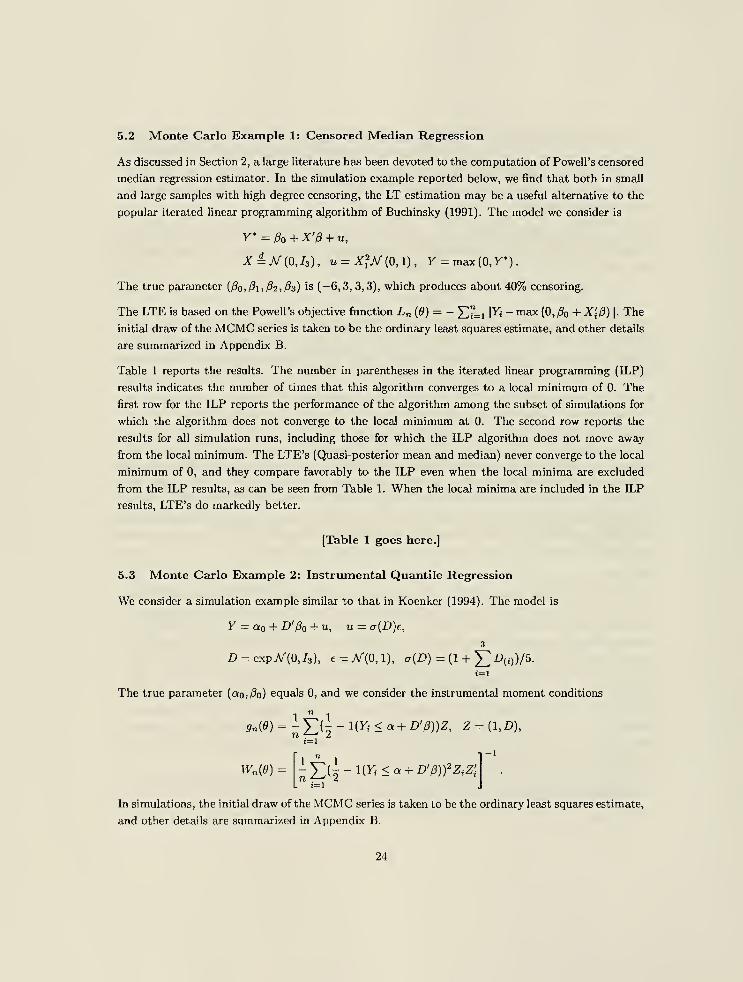
5.2 Monte Carlo Example 1: Censored Median Regression

As discussed in Section 2, a large literature has been devoted to the computation of Powell's censored

median regression estimator. In the simulation example reported below, we find that both in small

and large samples with high degree censoring, the LT estimation may be a useful alternative to the

popular iterated linear programming algorithm of Buchinsky (1991). The model we consider is

Y* = 0o + X'B + u,

X=A/"(0,J3 ), w = X!2A^(0,l), y = max(0,Y*).

The true parameter (80,81,32,63) is (—6,3,3,3), which produces about 40% censoring.

The LTE is based on the Powell's objective function Ln (6») = - £"=1 \Yf - max (0, O + X\8) |. The

initial draw of the MCMC series is taken to be the ordinary least squares estimate, and other details

are summarized in Appendix B.

Table 1 reports the results. The number in parentheses in the iterated linear programming (ULP)

results indicates the number of times that this algorithm converges to a local minimum of 0. The

first row for the ILP reports the performance of the algorithm among the subset of simulations for

which the algorithm does not converge to the local minimum at 0. The second row reports the

results for all simulation runs, including those for which the ILP algorithm does not move away

from the local minimum. The LTE's (Quasi-posterior mean and median) never converge to the local

minimum of 0, and they compare favorably to the ILP even when the local minima are excluded

from the ILP results, as can be seen from Table 1. When the local minima are included in the ILP

results, LTE's do markedly better.

[Table 1 goes here.]

5.3 Monte Carlo Example 2: Instrumental Quantile Regression

We consider a simulation example similar to that in Koenker (1994). The model is

Y = a + D'Bo + u, u = a(D)e,

3

D = exptf(0,I3 ), e = AA(0,l), a(D) = (1 + £l>(o)/5.

The true parameter (ao,0o) equals 0, and we consider the instrumental moment conditions

l-i r 1

-E(2 _1(Yi - a+i?'

/?))2^''•

. t=i

In simulations, the initial draw of the MCMC series is taken to be the ordinary least squares estimate,

and other details are summarized in Appendix B.

24

Wn {0)

While instrumented median regression is designed specifically for endogenous or nonlinear models, we

use a classical exogenous example in order to provide a contrast with a clear undisputed benchmark

- the standard linear quantile regression. The benchmark provides a reliable and high-quality

estimation method for the exogenous model. In this regard, the performance of the LT estimation

and inference, reported in Table 2 and Table 3, is encouraging.

Table 2 summarizes the performance of LTE's and the standard quantile regression estimator. Table

3 compares the performance of the LT confidence intervals to the standard inference method for

quantile regression implemented in S-plus 4.0. The reported results are averaged across the slope

parameters. The root mean square errors of the LTE's are no larger than those of quantile regression.

Other criteria demonstrate similar performance of two methods, as predicted by the asymptotic

theory. The coverage of Quasi-posterior quantile confidence intervals is also close to the nominal

level of 90% in both small and large samples. It is also noteworthy that the intervals do not require

nonparametric density estimation, as the standard method requires.

[Tables 2 and 3 go here.]

6 An Illustrative Empirical Application

The following illustrates the use of LT estimation in practice. We consider the problem of forecasting

the conditional quantiles or value-at-risk (VaR) of the Occidental Petroleum (NYSE:OXY) security

returns. The problem of forecasting quantiles of return distributions is not only important for

economic analysis, but is fundamental to the real-life activities of financial firms. We offer an

econometric analysis of a dynamic conditional quantile forecasting model, and show that the LTEapproach provides a simple and effective method of estimating such models (despite the difficulties

inherent in the estimation).

The dataset consists of 2527 daily observations (September, 1986 - November, 1998) on

Yt , the one-day returns of the Occidental Petroleum (NYSE:OXY) security,

Xt , a vector of returns and prices of other securities that affect the distribution of Yt : a

constant, lagged one-day return of Dow Jones Industrials (DJI), the lagged return on the spot

price of oil (NCL, front-month contract on crude oil on NYMEX), and the lagged return Y(_i.

The choice of variables follows a general principle in which the relevant conditioning information

for estimating value-at-risk of a stock return, Xt , may contain such variables as a market index of

corresponding capitalization and type (for instance, the S&P500 returns for a large-cap value stock),

the industry index, a price of a commodity or some other traded risk that the firm is exposed to,

and lagged values of its stock price.

25

Two functional forms of predictive r-th quantile regressions were estimated:

Linear Model : Qn+1 (r|It , 9{tJ) = X't9(t),

Dynamic Model: (?yt+1 (r|/€ ,»(r),e(r)) = X't9{r) + q(t) QYt [r\It-i,9{r),Q{r)),

where QYt+1 {T\h , 9(t)) denotes the r-th conditional quantile of Yt+i conditional on the information

It available at time t. In other words, Qyt+l (r|J(,0(r)) is the value-at-risk at the probability level

t. The idea behind the dynamic models is to better incorporate the entire past information and

better predict risk clustering, as introduced by Engle and Manganelli (2001). The nonlinear dynamic

models described by Engle and Manganelli (2001) are appealing, but appear to be difficult to estimate

using conventional extremum methods, see Engle and Manganelli (2001) for discussion. An extended

empirical analysis of the linear model is given in Chernozhukov and Umantsev (2001).

The LT estimation and inference strategy is based on the Koenker and Bassett (1978) criterion

function,

n

Ln (9,e) = -Y,MT)PT(Yt-Q Yt (T\it-u e, e)), (e.i)

t=s

where pT (u) — (t — l(u < 0))m. This criterion function is similar to that described in Example 1,

with the exception that there is no censoring. The starting value s = 100 initializes the recursive

specification so that the imputed initial conditions (taken to be the marginal quantiles) have a

numerically negligible effect.

In the first step, we constructed the LT estimates using the flat weights

wt (r) = 1/t(1 — t) for each t — s,...,T.

The results of the first step are not presented here, but they are very similar to those reported

below. Because the weights are not optimal, the information equality does not hold, hence Quasi-

posterior quantiles are not valid for confidence intervals. However, the confidence intervals suggested

in Theorem 4 lead to asymptotically valid inference. Under the assumption of correct dynamic

specification, stationary sampling, and the conditions specified in Proposition 3, the LTE's are

consistent and asymptotically normal

(?(r)i(r)')^^(0,J(9o)- 1

"(«o)J(Co)-i

) , (6.2)

where for V<?t (r) = dQYl {r\It-i,Q{r),9{r))ld{Q,9')' and qt (r) = Qn (r\It-i,e(r),9(T)),

J(9 ) = EfYtlIt_Mt(T))Vqt (T)Wqt (r)',

and for ^M = -^= ^L, fr~ Iff < *(t))] V ft (r),

fl(0o) = l™ ^—£An (0o)A n (0o )' - r(l - rJEVftWVftW'.T->co J — S

If the model is not correctly specified, then, for example, the Newey and West (1987) estimator

provides a consistent and robust procedure for estimation of the limit variance Q{9 ).

26

The estimation of the matrix J(#o)-1 can be done through the use of nonparametric methods as in

Powell (1984). Alternatively, as suggested in Theorem 4, we can use the variance-covariance matrix

of the MCMC sequence of parameter draws multiplied by n = (T — s) as a consistent estimate of

J(6a)~x

. Plugging the estimates into the variance expression (6.2), we obtain the standard errors

and confidence intervals that are qualitatively similar to those reported in Figures 4-7.

In order to illustrate the use of Quasi-posterior quantiles (Theorem 3) and improve estimation

efficiency, we also carried out the second step estimation using the Koenker-Bassett criterion function

(6.1) with the weights

ffi(, h 1__

[QYt(T + h/2\it- 1 ,e{T),e{T))-QYt

{T-h/2\it.u e(T),9{T))]' t(i-t)'

where h oc Cn~ x lz and C > is chosen using the rule given in Koenker (1994). Under the assumption

of correct dynamic specification, these weights imply the generalized information equality, which

validates Quasi-posterior quantiles for inference purposes, as in (4.12)-(4.16). The following analysis

is based on the second step estimates. The .05-th, .5-th, and .95-th Quasi-posterior quantiles are

computed for each coefficient 0j{t) (j = 1, ...,4) and £>(t), and then used to form the point estimates

and the 90%-confidence intervals, which are reported Figures 4-7 for r = .2, .4, ..., .8.

Figures 2 and 3 present the estimated surfaces of the conditional VaR functions of the dynamic model

and linear models, respectively, plotted in the time-probability level coordinates, (i,p), (p — t is the

quantile index.) We report VaR for many values of r. The conventional VaR reporting typically

involves the probability levels at a given r. Clearly, the whole VaR surface formed by varying r

represents a more complete depiction of conditional risk.

The dynamics depicted in Figures 2 and 3 unambiguously indicate certain dates on which market

risk tends to be much higher than its usual level. The difference between the linear and the recursive

model is also striking. The risk surface generated by the recursive model is much smoother and is

much more persistent. Furthermore, this difference is statistically significant, as Figure 7 shows.

Focusing on the recursive model, let us examine the economic and statistical interpretation of the

slope coefficients ^(0> ^3(')> #4(')> ?(')> plotted in Figures 4-7.

The coefficient on the lagged oil price return, #2(-)> is insignificantly positive in the left and right

tails of the conditional return distribution. It is insignificantly negative in the middle part. The

coefficient on the lagged DJI return, 03(-), in contrast, is significantly positive for all values of r. Wealso notice a sharp increase in the middle range. Thus, in addition to the strong positive relation

between the individual stock return and the market return (DJI) (dictated by the fact that #2(-) >

on (0.2,0.8)) there is also additional sensitivity of the median of the security return to the market

movements.

The coefficient on the own lagged return, 6><i(-), on the other hand, is significantly negative, except

for values of t close to 0. This may be interpreted as a reversion effect in the central part of the

distribution. However, the lagged return does not appear to significantly shift the quantile function

in the tails. Thus, the lagged return is more important for the determination of intermediate risks.

27

Most importantly, the dynamic coefficient g () on the lagged VaR is significantly negative in the low

quantiles and in the high quantiles, but is insignificant in the middle range. The significance of q(-)

is a strong evidence in favor of the recursive specification. The magnitude and sign of g(-) indicates

both the reversion and significant risk clustering effects in the tails of the distribution (see Figure

7). As expected, there is zero effect over the middle range, which is consistent with the random walk

properties of the stock price. Thus, the dynamic effect of lagged VaR is much more important for

the tails of the quantile function, that is for risk management purposes.

7 Conclusion

In this paper, we study the Laplace-type Estimators or Quasi-Bayesian Estimators that we define

using common statistical, non-likelihood based criterion functions. Under mild regularity conditions

these estimators are v^-consistent and asymptotically normal, and Quasi-posterior quantiles provide

asymptotically valid confidence intervals. A simulation study and an empirical example illustrate

the properties of the proposed estimation and inference methods. These results show that in many

important cases the Quasi-Bayesian estimators provide useful alternatives to the usual extremum

estimators. In ongoing work, we are extending the results to models in which v^-convergence rate

and asymptotic normality do not hold, including the maximum score problem.

Acknowledgments: We thank the editor for the invitation of this paper to Journal of Econometrics

and an anonymous referee for prompt and highest quality feedback. We thank Xiahong Chen, Shawn

Cole, Gary Chamberlain, Ivan Fernandez, Ronald Gallant, Jinyong Hahn, Bruce Hansen, Chris

Hansen, Jerry Hausman, James Heckman, Bo Honore, Guido Imbens, Roger Koenker, Shakeeb Khan,

Sergei Morozov, Whitney Newey, Ziad Nejmeldeen, Stavros Panaceas, Chris Sims, George Tauchen,

and seminar participants at Brown University, Duke-UNC Triangle Seminar, MIT, MIT-Harvard,

University of Chicago, Princeton University, University of Wisconsin at Madison, University of

Michigan, Michigan State University, Texas-AM University, the Winter meeting of the Econometric

Society, the 2002 European Econometric Society Meeting in Venice for insightful comments. Wegratefully acknowledge the financial support provided by the U.S. National Science Foundation

grants SES-0214047 and SES-0079495.

A Appendix of Proofs

A.l Proof of Theorem 1

It suffices to show

\h\°\p'n (h)-pUh)\dh-> p (A.l)/,.

for all a > 0. Our arguments follow those in Bickel and Yahav (1969) and Ibragimov and Has'minskii

(1981), as presented by Lehraann and Casella (1998). As indicated in the text, the main difference are in

part 2, and are due to (i) the non-likelihood setting, (ii) the use of Huber-like conditions in Assumption 4

to handle discontinuous criterion functions, (iii) allowing more general loss functions, which are needed for

construction of confidence intervals.

28

Throughout this proof the range of integration for ft is implicitly understood to be Hn . For clarity of the

argument, we limit exposition only to the case where J„(9) and Q„(9) do not depend on n. The more general

case follows similarly.

Part 1. Define

then

ft = v^(0 - Tn ) , T„ = O + -J {Bo)-' A„ (0O ) , Un = -^J(9 )-' A„(0O ),n ^/n

p„ (ft) =—=p„ (fc/v^ + 5o + Un/Vn)

where

and

/»„ w (^ + T") exP(L" (^ + T")) dh

*(jz + Tn)exp(u>(h))

^7r(^ + T„)exp(w(ft))"

a,'

w (ft) = L„ (V„ + 4= )- L (0o) - ^-A„ (0O )' ^ (flo)"' A„ (0O )

,

Cn = [ ix (-y= + Tn \ exp (w(ft)) dft.

Part 2 shows that for each o > 0,

A,„= /"|ft|

aexp(w(ft))7rfrn + jLj-expf-|ft'J(0o)ft)7r(0o )

Given (A.4), taking a = we have

C„->„ f e-^'-,(9o "l

7r(0o)dft = 7r(0o)(27r) = |detJ(0o)r1/2

dft -^0.

hence

Next note

left

C„ =Op (l).

side of (A. 1) ee / |ftHpn (ft) -p^(ft)|dft = >1„ C„-\

i-here

4„ = /" |ft|° ewW Tr(Tn + -j=} - {2-K)-

dl7\<\etJ (0O )|

,/2 exp f-h' J (9 )h\ C„ dh.

Using (A. 5), to show (A.l) it suffices to show that A n -?-y 0. But

A„ < A\„ + A 2„

(A.2)

(A.3)

(A.4)

(A.5)

29

where

A2n = J\h\

a C„(2Ky d/2\detJ(0o)\

l/2 exp(-^h'J(6o)h\ -is (0o)exp (~h'J(e )h\

Then by (A.4)

dh.

0,

and

A2„ = C„(27r)-d/2

|det J(0O) |

1/2 - tt(0o)

0.

f \h\"ex.p(-^h'j(9o)h\dh

Part 2. It remains only to show (A.4). Given Assumption 4 and definitions in (A. 2) and (A. 3), write

- ^An (0O)' J (flo)-1 An (fl ) + Rn (-^= + T„)

= -\tiJ{e )h + Rn (^= + T„Y

Split the integral A\„ in (A.4) over three separate areas:

• Area (i) : \h\ < M,

• Area (ii) : M < \h\ < 8y/n,

• Area (Hi) : \h\ > 8y/n.

Each of these areas is implicitly understood to intersect with the range of integration for h, which is H„.

Area (i): We will show that for each < M < oo and each e >

liminf P.l f \h\c exp(w(h))n(Tn + —=j

-exp(-^tij{0o)h\ir(eo ) dh < e | > 1 - .

(A.6)

This is proved by showing that

exp(to (ft))* \T„ + -M -exp (~h'J(9o)h\ tt(5)

Using the definition of uj(h), (A. 7) follows from:

sup|

\h\<M(A.7)

(a) sup\h\<M

n(^=+Tn ) -7z(S ) -Ao, (6) sup \R^(-^=+Tn)\v« / \h\<M\ VV" /o,

where (a) follows from the continuity of ir(-) and because by Assumption 4.ii-4.iii:

1

y/ZJ(flo)" ' A„ (fl ) = Op (1) (A.8)

30

Given (A.8), (b) follows from Assumption 4.iv, since

hsup\h\<M

Tn H

—

= — 9o = Op{l/Vn).

Area (ii): We show that for each e > there exist large M and small 5 > such that

Iiminf P. < /" [Jm< \k\<5s/^

exp (w (h)) k (**)- exp (- ]rtiJ{8 ) h\ -k (8 ) \dh< e 1

(A.9)

> 1 -€.

Since the integral of the second term is finite and can be made arbitrarily small by setting M large, it suffices

to show that for each e > there exist large M and small 5 > such that

Iiminf P.l I[Jm< \h\<SJK

W exp(w(h))n (t„ + -=) hdh < e > > 1 - e

In order to do so, it suffices to show that for sufficiently large M as n —> oo

exp (w (k)) 7r (T„ + -^= j< C exp (-jh'J (8 ) h\ , for all M < \h\ < 5y/n.

By assumption 7r (•) < K, so we can drop it from consideration.

By definition of ui(h)

exp (w (h)) < exp[- -ti J (8 ) h + Rn (* + £)

Since \T„ — 8\= op (l), for any 5 > wp —> 1

< 25, for all \h\ < 5y/n.

Thus, by Assumption 4.iv(a) there exists some small 5 and large M such that

T„ H

—

-= — Bo

Iiminf P.', < sup\ M<\h\<&

< ^mineig (J (8 )) \ > 1 - e.

lsV*\h+^J(8o)- 'A„(9 )|2 " 4

Since ^\J (Bo)'1 A„ (8 )

|

2 = Op (1), for some C >

lim inf P. i exp(u>(h)) < Cexp (-jft'j(A)fcH

> liminfpJe"'" < Cexp (-hi J(8 )h+ -mineig (J (Bo)) \h\

0}> 1-e.

(A. 12) implies (A. 11), which in turn implies (A.9).

(A.10)

(A.H)

(A.12)

31

Area (iii): We will show that for each e > and each 8 >

limlinfP.i f |h|a|exp(u;(/i))irfrn + 4=

>

)

- exp (~tiJ(e )h\ n{9 ) \dh < e I

The integral of the second term clearly goes to as n —> oo. Therefore we only need to show

f \h\ae"wn (T„ + JL) dh-+ p 0.

J|/.|>iiv^ V v n /

Recalling the definition of h, the term is bounded by

vr +i[J\e

(A.13)

> 1-e.

Tn -9 ,r ((9) .-x,>jLn (9) - Ln (9 )

- ^ A„ (So)' J (do)-1 An (0O )

J

d6.

-T„|>J

Since T„ — 9o -^4 0, wp -> 1 this is bounded by

X„ C • %/Ha+1

/ (1+ \9\

a) -k (6) exp (L„ (6) - i„ (0O)) e»,

•/|9-»ol>«/2

where

isT„ = exp f-^A„ (%)' J^o)"1 A„ (9 )j

= Op (l).

By Assumption 3 there exists e > such that

liminfpj sup eL"m - L" l,a) < e"e

} = 1

Thus, wp —> 1 the entire term is bounded by

#„ • C ^/n,+1

• e~n'

f \9\a

ir (9) d0 = op (l). (A.14)

Here observe that compactness is only used to insure that

[ \6\a Tx{9)d9<oo. (A.15)

Hence by replacing compactness with the condition (A.15), the conclusion (A.14) is not affected for the given

a.

The entire proof is now completed by combining (A. 6), (A. 9), and (A.13).

A.2 Proof of Theorem 2

For clarity of the argument, we limit exposition only to the case where J„ (9) and fi„ (9) do not depend on

n. The more general case follows similarly.

Recall that

h = y/n{9-6 )-J (So)"1 An (g ) /y/n.

32

£ = arg infI6» d

I jRd'

Define Un = J(do)l

&n{8o)Iy/n. Consider the objective function

Qn (z) = J p(z-h- U„)p*n (h)dh,

which is minimized at ^/n(8 — 80) Also define

Q<x>(z) = / p{z - h - U„)p*x {h)dh.Jr*

which is minimized at a random vector denoted Zn . Define

lj^p(z-h) PUh)dh\.

Note that solution is unique and finite by Assumption 2 parts (ii) and (iii) on the loss function p. When pis symmetric, f = by Anderson's lemma.

Therefore, Z„ — arg infzift d Qae(z) equals

Zn = £ + !/„ =Op (l).

Next, we have for any fixed z

Qn(z) - Q ao{z)^v

since by Assumption 2.H p(h) < 1 + \h\p and by \a + b\

p < 2p~ l

\a\p + 2p

- 1

|6|p for p > 1:

\Qn(z)-Q ao (z)\< f (X + \z-h-U„\n\Pn{h)-pUh)\dh

+ [ (l + \z-h-Un n<plo(h))dh

< f {l+2p- i

\h\p +2p- l \z-U„\p

)\p'n {h)-p'ao {h)\dhJh„

+ f (l + 2p- ,

\h\p + 2p

- 1\z-U„\ p)(p-ao (h))dh

< [ (l+2p-'\h\ p +Op (l))(p'n (h)-pUh))dh

+ f (l + 2»-'\h\ p + Op(l))(pUh))dh = op (l),

where op(l)-conclusion is by Theorem 1 and exponentially small tails of the normal density (Lebesgue

measure of H„ converges to zero).

Now note that Qn {z) and Qaa(z) are convex and finite, and Z„ = arginfzgR i Qac(z) = Op (l). By the

convexity lemma of Pollard (1991), pointwise convergence entails the uniform convergence over compact sets

K:

sup <2„(z) - Qoc(z) ->„ 0.

Since Zn = Op (l), uniform convergence and convexity arguments like those in Jureckova (1977) imply that

yjn(8 — 80) — Z„-> p 0, as shown below.

Proof of Zn — yfn(8 — 80) = op (l). The proof follows by extending slightly the convexity argument of

Jureckova (1977) and Pollard (1991) to the present context. Consider a ball Bs(Z„) with radius 5 > 0,

33

centered at Zn , and let z = Zn + dv, where visa unit direction vector such that \v\ = 1 and d> 8. Because

Z„ = Op (l), for any 8 > and e > 0, there exists K > such that

liminf P.iE„ = {BS (Z„) S BK (0)}\ > 1 - e.

By convexity, for any z = Zn + dv constructed so, it follows that

^(Q-OO - Qn{Zn )) > Qn (z') - Q„(Z„), (A.16)

where z* is a point of boundary of Bs{Zn ) on the line connecting z and Z„. By the uniform convergence of

Q„(z) to Qoc(z) over any compact set ZJk-(O), whenever En occurs:

^(Qn(z) - Q„(Z„)) > Q„(z*) - Qn (Zn )

> Qoo(z*) - Qoc(^n) + Op (l) > V„ + Op (l),

where V„ > is a uniformly in n positive variable, because Zn is the unique optimizer of Q<x>- That is, there

exists an 77 > such that lim inf„ P(Vn > jj) > 1 — e. Hence we have with probability at least as big as

1 — 3e for large n:

2(Qn(z)-Qn (Zn))>71 .

Thus, yfn{9 — 9o) eventually belongs to a complement of Bs(Zn ) with probability at most 3e. Since we can

set e as small as we like by picking (a) sufficiently large K, and (b) sufficiently large n, and (c) sufficiently

small T) > 0, it follows that

iimsupP*{|z„ -V^{e-e )\ ><s} = 0.

Since this is true for any 8 > 0, it follows that

Z„ - Vn(9 - 9 ) = op (l). M

A.3 Proof of Theorem 3

For clarity of the argument, we limit exposition only to the case where J„(8) and iin {9) do not depend on

n. The more general case follows similarly. We defined

f„. b (z) = / Pn {e)d0.Jee&-.9 (,e)<x

Evaluate it at x = <?(#o) + sj^fn and change the variable of integration

H9As) = Fg ,„(9(So) + s/V^) = fp'n (h)dh.

Define also

Sg ,n (s) =

//.<ER'<: 9 (0o+'i/v/n+ k%./v/5r)<s(9o)+s/%Af

8g ,n (s) = / p'ooWdh

JheR d:g(e +h/ w^+Un /^r)<g(8 )+3/^;

Hg ,oo(s) = / plcitydh.J/.6R J:Vor9nVf/i/VS"+U„/v^r)<s/v^

and

Hg^is) =//.eR J :V9(9 )'('i/v^'+t''n/v^)<»/yS

34

By definition of total variation of moments norm and Theorem 1

sup \Hg>„(s) - H3 ,„(s)|-»-p 0,a

where the sup is taken over the support of Hg<n (s).

By the uniform continuity of the integral of the normal density with respect to the boundary of integration

sup|i?s,„(s) --ff9,oo(s)|->p 0,

which implies

SUp |ifg,„(s)- -ff3,oo(s)|->p 0.

3

where the sup is taken over the support of H3i„(s).

The convergence of distribution function implies the convergence of quantiles at continuity points of distri-

bution functions, see e.g. Billingsley (1994), so

i?-i (a) - ff-^ (<*)-„ 0.

Next observe

ff9 ,oo(s) = P{^g(Bo)'N'(Un , J-'iBo)) < s\un },

H~Ua) = Vg(9 )'Un + qa ^Vgg(Bo)'J-, (BoWeg(0o),

where qa is the a-quantile of jV(0, 1).

Recalling that we denned c3 ,n(aO = F~l(a), by quantile equivariance with respect to the monotone trans-

formations

tf-i(a ) = yS(cs,„(a)-ff(0o))

so that

\/n(cg ,„(a) - g(6 )) = Vg{6Q)'Un + g V^»9W^W»sW + <'p(l)-

The rest of the result follows by the A-method.

A.4 Proof of Theorem 4

In view of Assumption 4, it suffices to show that

Jn\6 )- J„

_,(e )->p 0, (A. 17)

and then conclude by the A-method.

Recall that

h = VS(0 - B )- Jn (So)

-1 A„ (Bo) A/S,

u„

and the localized Quasi-posterior density for h is

p*n (h) = —p„ (h/y/n + 0o + U„/y/n) .

yTl

35

Note also

J"1

(Bo) = J n{9- 9)(9 - 0)'pn (9)d9

= J (h-V^(9-6o) + Un )-(h-VE(e-8 )+Un yp:t(h)dh,

and

J~l

{9o)= J htiplcitydh.

We have, denoting h = (hu ..., dd ) and f„ = (f„i , ..., f„d ) where f„ = y/n{9 - 9 ) - U„ , for all i, j < d

(a) fHn hihj (p'n (h) -ploihijdh = op (l) by Theorem 1,

(b) fHC hihj [plo(h)jdh = op (l) by definition of pjo and Jn {9o) being uniformly nonsingular,

(c) fHn \fn\

2(p'n (h) -pUh))dh = op (l) by Theorem 2,

=<.„(!)

(d) /H \Tn\

2(ploihndh = op (l) by Theorem 2, definition of p^,, and Jn (9o) being nonsingular,

(e) JHri hj fni (p'„(h) - plcihijdh = op (l) by Theorems 1 and 2,

=°„(i)

(f) /H fcj T„i (p£oC0 )dh = op (l) by Theorems 1 and 2, definition of p'^, and J„(5o) being uniformly

nonsingular, from which the required conclusion follows.

A.5 Proof of Proposition 1

Assumption 3 is directly implied by (4.1)-(4.4) and the uniform continuity of Errii (8), as shown in Lemma1. It remains only to verify Assumption 4.

Define the identity

L„(8) - Ln (9 ) = - ngn (9 )'W{9 )G{8 ) {9 - 9 )

A„(fl )<

1(A.18)

--(9-9o )'nG{9oyw(9o)G(0o)(9-9o) + Rn (9).

Jtfo)

Next, given the definition of A n (9o) and J(9o), conditions i, ii, iii of Assumption 4. are immediate from

conditions i-iii of Proposition 1. Condition iv is verified as follows. Condition iv of Assumption 4 can be

succinctly stated as:

ii ID (Q\ I~)

for each e > there exists a 8 > such that lim supP* < sup ——7-:— 1 ,„ > e > < 6.

36

This stochastic equicontinuity condition is equivalent to the following stochastic equicontinuity condition,

see e.g. Andrews (1994a):

id fa\ I

forany<5n ->0 sup 'v n = o„(l). (A.19)

|»—

e

l<<5„l + n|ff — flop

This is weaker than condition (v) of Theorem 7.1 in Newey and McFadden (1994), which requires

sup"T^ifl fl i, „i/)—FT? = °pW > (A. 20)

Rn(9) Rn{6) \VE\9-e \+n\d-9 \'

l + n|0-0o|

2 Vn\6 - 0o | + n\9 - O|

2L l + n|0-0o

|

2

where the term in brackets is bounded by

v^ie - g|

"*"

l + rc|0-0o|

2 -

Hence the arguments of the proof, except for several important differences, follow those of Theorem 7.2 in

Newey and McFadden (1994).

At first note that condition iv of Proposition 1 is implied by the condition (where we let g(9) = Egn (0)):

sup e (0) = ov(-L)

, where e (0) = 3" ^ ~ 9"f*

o) =f<*>

for any ft. -> 0. (A.21)»6Bjn (eo) Vv™/ 1 + Vn|0-0O

|

v ;

From (A. 18)

fl* (0) = i?m(0) + «2n (0) + Rsn(6),

where

Rln (0) =n (gn (0O )' W„ (0)G (0O ) (0 - 0o) + \ (0 - 0o)' G (0O )' W(9)G (0O) (0 - 0o)

- 5* («)' W»(%« (0) + \g„ (Bo)' W„(%„ (00)) ,

iZ2„ (0) ="Qs» (0o)' (W„(0o) - iy„(0)) 9„ (0o)) ,

R3n (9) =n(gn (flo)' (W(6 ) - W„(fl))) G (0O ) (0 - 0o)

+ \(9- 0o)' G (0O )' (W(9 )- W(9)) G (0O ) (0 - 0o))

.

Verification of (A.19) for the terms R2„{9) and Rin immediately follows from y/ng„(6 ) = Op (l) and the

uniform consistency ofWn (9) in as assumed in condition i of Proposition 1 and from the continuity of W(9)

in by condition i of Proposition 1, so that W„(0) - W(9) = op (l) uniformly in and W(9) - W(9 ) = o(l)

as |0 - O |

-> 0.

It remains to check condition (A.19) for the term Ri„(0). Note that

<?„ (0) = (1 + y/H\9 - 0o|) 6 (0) +g(9) + gn (0O ) .

37

Substitute this into Ri„ (9) and decompose

- -Rm (6) = I (1 + Vn|« - 6o\)2e (0)' W„(0)e (0) +gn (9 )' W„(9)(g (9) - G (9 )) (9 - 9

)

+ (1 + V^|fl - flo|) e (0)' W„(<%- (fl ) + (1 + V^\9 - 9 \) e (9)' Wn (9)g (9)

+ \g («)' (Wn (9) - W(9)) g (9) + \g (9)' W(9)g (9) -\{9 - 9 )' G (9 )' W(9)G (0O ) (9 - 9 )

.

Using the inequalities, for x > 0:

(1 + y/nxf < 2y/iii

< 11 + Vni

< 2n (1 + y/ng)

<^y/n

(A.22)1 + ra2

' ' 1 + nx 2 ~ ' 1 + nx2 —1 +m2 —

x'

each of these terms can be dealt with separately, by applying the conditions i- iii and (A.21):

(a) sup .,W|

7fl

(0)i i2 < SUP ne(9)'Wn (9)e(9)=op (l),

(6) sup '

v '' = sup - v * ' W„ (9)v^3n (00) = op (1)

,

9es 5„(eo) :

+

"l0_£/°l 9eB 5„(e ) 1 + n|0 - »or

<c) SUPi u"

1

?/^ 12 ^ SUP 2n| e (0)'W.(«)ff»(*o)| = Op(l).

(d) sup - "'? W ' < sup 2^ eWW-Wi/^- = °p(1),

(e) supi + 1?/" P * sup &(«)-^)l = MD,

»6B 5„(»o)1 +n

\

(> -Vo\' 9€B S„(8 ) I

8 -9°\

,« "Mfl)| ^ O (|e-9o|2

|^(g)l)

C6Bj„(»o) l + nlC-Por e6B ire (e )\o-0or

where (a) follows from (A.22), (A.21), and condition i, which states that Wn {9) = W{9) + op (l) and

VK(0) > is finite uniformly in 9; in (b) the first equality follows by Taylor expansion g(9) = G (9o) {9 — 9o) +o{\9 — 9o\) and the second conclusion follows from (A.22) and condition iii; (c) follows from (A.22), (A.21),

condition i and iii; (d) follows by (A.22) and then replacing, by condition ii, g{9) with G (9o) {9 — 9o) 4-

o(\9 — 6o\), followed by applying (A.21) and condition i; (e) follows from replacing by condition ii g(9)

with G (9o) (9 — 9o) + o (\9 — 9o\), followed by applying condition i; and (f) follows from replacing g (9) with

G(9o) (9 — 9o) + o(\9 — So I),followed by applying condition i.

Verification of (A. 20) for the term R\ n {9) now follows by putting these terms together.

A.6 Proof of Proposition 2

Verification of Assumption 3 is standard given the stated conditions and is subsumed as a step in the

consistency proofs of extremum estimators based on GEL in Kitamura and Stutzer (1997) for cases when s

is finite and Kitamura (1997) for cases when s takes on infinite values. We shall not repeat it here. Next,

38

we will verify Assumption 4. Define

7(0)=arg mfL„(0, 7).

It will suffice to show that uniformly in 9„ 6 Bgn (9o) for any <Jn —> 0, we have the GMM set-up:

Ln (9„)=Ln (9„,T{9n ))

1 / 1 " V ,/i" "\ (A.23)

where

V(0o) = Erm {9 ) rm (9 )'

.

The Assumptions 4.i-iii follow immediately from the conditions of Proposition 2, and Assumption 4.iv is

verified exactly as in the proof of Proposition 1, given the reduction to the GMM case. Indeed, defining

gn (9) = ^5D"_, mi(9), the Donsker property assumed in condition iv implies that for any e > 0, there is

S > such that

limsupPV sup -/R\gn (9) - gn {9 ) - (Egn (9) - Eg„(9 ))\ > e\ < e,

n-too (eeB s (e ) )

which implies

,- „. J V^\9n{9) - g„(9o) - (Egn (9) - Eg„(9 ))\ \limsupP < sup -— —-— _ — > e f < ei

n-»oo [esfljfSo) 1 +

v

n l" — "o|J

which is condition iv in Proposition 1. The rest of the arguments follow that in the proof of Proposition 1.

It only remains to show the requisite expansion (A.23). We first show that

W.H 0.

For that purpose we use the convexity lemma, which was obtained by C. Geyer, and can be found in Knight

(1999).

Convexity Lemma. Suppose Qn is a sequence of lower-semi-continuous convex R-valued random functions,

defined on Rd, and let 2? be a countable dense subset of $&

d. If Qn weakly converges to Qoo in R marginally (in

finite-dimensional sense) on V where Qoo is lower-semi-continuous convex and finite on an open non-empty

set a.s., then

arginf Qn (z)-+d arginf Qoo(z),

dprovided the latter is uniquely defined a.s. in R

Next, we show that 7(6n )-*p 0. Define F = {7 : £s[m,(0o)'7] < 00} and Fc = {7 : Es{mi{9o)'l] = 00}.

By convexity and lower-semicontinuity of s, F is convex, open, and its boundary is nowhere dense in Rp.

Thus for 7 e F, Es[mi(9)''y] < 00 for all 9 € Bs(9o) and some 5 > 0, which follows by continuity of

9 >-> Es[mi(9)'y] over Bs{9o) implied by the condition ii and iii.

Thus, for a given 7 6 F and any 9n —

>

p 9a

1 "-Y"s[mi(B„)'y]-> p Es[Tni(9o)'i] < 00.77 ' »

39

This follows from the uniform law of large numbers implied by

1. {s[mi(9)'f],8 6 Bs{9o)}, where S is sufficiently small, being a Donsker class wp -+ 1, and

2. Em.i{8) = J x dP\rn,i{9) < x] being continuously differentiable in 9 by condition ii and iii.

The above function set is Donsker by

(a) m,(0)'7 £ M for some compact M and a given 7 E F, by condition iii,

(b) {mi(6),6 £ Bs(0o)} being Donsker class by condition iv,

(c) s being a uniform Lipschitz function over V Pi M 17, by assumption on s,

(d) mi(S)'7 e V for all 9 £ B}(9o), some S > 0, and a given 7 e F, by construction of F,

(e) Theorem 2.10.6 in van der Vaart and Wellner (1996) that says a uniform Lipschitz transform of a

Donsker class is Donsker class itself.

Now take 7 in Fc\ dF, where dF denotes the boundary of F. Then wp —> 1

1 ™— 7^ s[mi(9nYj] = 00—

>

p Es[mi(9oY"i] = 00.n ^—

'

Now take all the rational numbers 7 e Rp\ dF as the set T> appearing in the statement of the Convexity

Lemma and conclude that

7(0")-»p = arg inf7Fs[7n,(9o)'7].

Given this result, we can expand the first order condition for 7(0„) in order to obtain the expression for its

form. Note first

= J^ Vs (7 (9n)' mi (0„ )) m, (<?„)

'':'(A-24)

where

V» = -V V 2s (7 (9n )' m, (9n )) rrn (9n ) mi (0„)'

,

T7. *—

»

for some 7(9n ) between and f{9„), which is different from row to row of the matrix Vn .

Then

V„-+ p V(6>o) = Fm, (9 ) m, (9 )'

.

This follows from the uniform law of large numbers implied by

1. {V2s(-y'mi(9*))mi(9)mi(9)' ,(0*,-y,9) 6 £,5,(00) x Bj2 (0) x B53 (9 )}, where 8

}> are sufficiently

small, being a Donsker class wp —> 1,

2. Emi(9)mi(9)' = J xx'dP[mi(9) < x] being continuous function in 9 by condition i,

17Recall that V is defined as the open convex set on which s is finite.

40

3. EV 2s(~f'mi (9"))mi (9) nu (9)' = £V2

s(0)77ii (9) tth (9)' + o(l) uniformly in (9, 9') e Bg(9 ) x B5 (9 ) for

sufficiently small 5 > 0, for any 7 —> 0, by assumptions on s and condition iii.

The claim 1 is verified by applying exactly the same logic as in the previously stated steps (a)-(e). For the

sake of brevity, this will not be repeated.

Therefore, wp — 1

-y(9n ) = -(Vn )- ,

^J2m i (9n ) = -(V(9 )- 1 +op(l))^J2mi (9n ). (A.25)

1=1 t=i

Consider the second order expansion,

i»(9«,7(«»))=Vwr(«»)' 4=y><(0-)+5V^(0»)'V»V«7(*»), (A.26)v" ,=1

l

where1 «^

V„ = - Y, V2s (7 (9r,)' m, (9n )) rm (9„) m,- (0n )'

,

for some 7 (9„) between and 7 (9n ), which is different from row to row of the matrix Vn . By a preceding

argument,

V„->P V(9 ).

Inserting (A.25) and V„ = V(9o) +op (l) into (A.26), we obtain the required expansion (A. 23).

A.7 Proof of Proposition 3

Assumption 3 is assumed. We need to verify Assumption 4.

Define the identity

Ln (9) - L„(9 ) = J2 mi(9o)'(9 - 9 )

1 (A.27)+ -(9 - 9 )'nyee,Em t (9 ) (9 - 9 )

-./(So)

+ Rn(9).

Assumption 4.i-iii then follows immediately from conditions i and ii. Assumption 4.iv is verified as follows.

The remainder term R„ (9) is given the following decomposition:

n

Rn (9) = J2 [m,{9) - m,(0o ) - Emi{9) + Emi(9 ) - m,(9 )'(9 - O)}

+ n{Em,{9) - Em t (9 )) + i(0 - 9 )'nJ(9 ){9 - 9Q )

.

k2„(S)

41

It suffices to verify Assumption 4.iv separately for Ri„(9) and R2„(9). Since

R2n(9) = -\n{6 - 6o)' \J(9") - J(9 )] (9 - 9 ),

for some 9" on the line connecting 9 and 9o, verification of Assumption 4 for R2n(9) follows immediately

from continuity of J(9) in 9 over a ball at 9o-

To show Assumption 4.iv-(b) for R\n {9), we note that for any given M >

limsupP*< sup |.Ri„(0)|>el" \\e-e \<M/jz J

<limsuPp| supl

9 -^! 1^'"^, 1 >el (A.28)" \\e-e \<M/^i \o — Oo\

J

<limsupW sup — LJiLkZJ >e}=0,

where the last conclusion follows from two observations.

First, note that

i{9) - mi (g )- (Erm{9) - Ermifio)) - mi{9 )'{9 - 9 )

"

z»w=^l

9-9 \-7nhyis Donkser by assumption, that is it converges in l°°(Bs(8o)) to a tight Gaussian process Z.

The process has uniformly continuous paths with respect to the semimetric p given by

p2{9u 92 ) = E{Z{9,) - Z{92)f

,

so that p{9,9) —> if 9 -* 9o- Thus almost all sample paths of Z are continuous at So-

Second, since by assumption

E[mn (9) - mn {9 ) -m^{8 )'(6 - 8 )]

2 = o{\9 - 9\

2),

we have for any 9n —> So

therefore

|-Ri„ (9n ) |

yfr\6n - So|

oJ^-9^|e„-e p

'

Z(flo) = o.

Therefore for any ff—> p So, we have by the extended continuous mapping theorem

Z„(6')-t d Z{9 ) = 0, that is Z„(9')-*p 0. (A. 29)

This shows (A.28).

To prove Assumption 4.iv-(a) for Rj„(9), we need to show that for some 5 > and constant M

limsupP-( sup'f

'" (

!11 > 4 < € (A.30)

42

Using that M/^/n < \9 — 9o\, bound the left-hand-side by

limsupP < supi-\a a i

' l~\a a~\ > €I

\RlnW\

M/^<\e-e \<5 i/n\8 - &o\ y/n\9 - 9\

< limsup P*'-'"

" '•"

(A.31)

,, fsu

[gin (9)| J_ > 1

\M/v^<|9P-9ol<*V'"|0- fl°l

MJ

< limsup P* J sup |Z„(0)| . J- > E L

n [m/vTT<|9-9oI<'5 ™I

where for any given e > in order to make the last inequality true, we can make either S sufficiently small

by the property (A. 29) of Z„ or make M sufficiently large by the property Z„ — Op . (1).

B Appendix on Computation

B.l A computational lemma

In this section we record some formal results on MCMC computation of the quasi-posterior quantities.

LEMMA 3 Suppose the chain (0 ',] < B) is produced by the Metropolis Hastings(MH) algorithm with q

such that q{8\9') > for each (6,9'). Suppose also that P{p(9u) ,£) = 1} > for all j > t . Then

1. pn () is the stationary density of the chain,

2. the chain is ergodic with the limit marginal distribution given by pn ()-"

B

where the supremum is taken over the Borel sets,

3. For any p„- integrable function g:

B

lim sup |p(0(B)

6 A\0o )- f pn {9)do\ = 0,

l-K» A \ JA I

JD^K f g(9)Pn (9)d9.

Proof. The result is immediate from Theorem 6.2.5 in Robert and Casella (1999).

An immediate consequence of this lemma is the following result.

LEMMA 4 Suppose Assumptions 1 and 2 hold. Suppose the chain {9 ,j < B) satisfies the conditions of

Lemma 3, then for any convex and p„-integrable loss function p„ (•)

arg infsee

provided that 9 is uniquely defined.

-,B 1 r r

nVp,^01 -0) ->p = arg inf / pn (0 - 8)pn (9)d9

43

Proof. By Lemma 3 we have the pointwise convergence of the objective function: for any 9

B

Bi

Br

^5>n(0 (i) -0)->„ / Pn(9-0)Pn(S)d9,

which implies the result by the Convexity Lemma, since 9 >-¥ J Pn(9 — 9)p„(9)d9 is convex by convexity of

B.2 Quasi-Bayes Estimation and Simulated Annealing

The relation between drawing from the shape of a likelihood surface and optimizing to find the mode of the

likelihood function is well known. It is well established that, e.g. Robert and Casella (1999),

[a 9eXL"mn(0)d9

xlim

f >l m LM = argmaxXn (9) (B.l)

Essentially, as A —> oo, the sequence of probability measures

eXL » (e

\(9)

J9 e* L-mn(9)d9

converges to the generalized Dirac probability measure concentrated at argmax L„ (9).see

(B.2)

The difficulty of nonlinear optimization has been an important issue in econometrics (Berndt et al. (1974),

Sims (1999)). The simulated annealing algorithm (see e.g. Press et al. (1992), Goffe et al. (1994)) is usually

considered a generic optimization method. It is an implementation of the simulation based optimization (B.l)

with a uniform prior ir (9) = c on the parameter space ©. At each temperature level 1/A, the simulated

annealing routine uses a large number of Metropolis-Hastings steps to draw from the quasi distribution

(B.2). The temperature parameter is then decreased slowly while the Metropolis steps are repeated, until

convergence criteria for the optimum are achieved.

Interestingly, the simulated annealing algorithm has been widely used in optimization of non-likelihood-based

semiparametric objective functions. In principle, if the temperature parameter is decreased at an arbitrarily

slow rate (that depends on the criterion function), simulated annealing can find the global optimum of

non-smooth objective functions that may have many local extrema. Controlling the temperature reduction

parameter is a very delicate matter and is certainly crucial to the performance of the algorithm with highly

nonsmooth objective functions. On the other hand, as Theorems 1 and 2 apply equally to (B.2), the

results of this paper show that we may fix the temperature parameter 1/A at a positive constant and then

compute the quasi-posterior medians or means for (B.2) using Metropolis steps. These estimates can be

used in place of the exact maximum. They are consistent and asymptotically normal, and possess the same

limiting distribution as the exact maximum. The interpretation of the simulated annealing algorithm as an

implementation of (B.2) also suggests that for some problems with special structures, other MCMC methods,

such as the Gibbs sampler, may be used to replace the Metropolis-Hasting step in the simulated annealing

algorithm.

B.3 Details of Computation in Monte-Carlo Examples

The parameter space is taken to be © = [9o ± 10]. The transition kernel is a Normal density, and flat

prior is truncated to 0. Each parameter is updated via a Gibbs-Metropolis procedure, which modifies

44

slightly the basic Metropolis-Hastings algorithm: for k = \,...,d, a draw of fit from the univariate normal

density q(\t,k — 9% \,<t>) is made, then the candidate value f consisting of ft and 8_ k replaces 0^') wjth

probability p(6^\^) specified in the text. Variance parameter<f>

is adjusted every 100 draws (in the second

simulation example and empirical example) or 200 draws (in the first simulation example) so that the

rejection probability is roughly 50%.

The first N x d draws (the burn-in stage) are discarded, and the remaining N x d draws are used in

computation of estimates and intervals. The starting value is the OLS estimate in all examples. We use

N = 5, 000 in the second simulation example and empirical example and N = 10, 000 in the second simulation

example. To give an idea of computational expense, computing one set of estimates takes 20-40 seconds

depending on the example. All of the codes that we used to produce figures, simulation, and empirical

results are available from the authors.

Notation and Terms

—

>

p convergence in (outer) probability P*—>d convergence in distribution under P*

wp —> 1 with inner probability P. converging to one

~ asymptotic equivalence denoted A ~ B means lim AB~ l = /

-Bj(x) ball centered at x of radius 8 >/ identity matrix

A > A is positive definite when A is matrix

A/"(0, a) normal random vector with mean and variance matrix a

J- Donsker class here this means that empirical process / >-* -4= 2™_i(/(Wi) — &f(Wi)) is

asymptotically Gaussian in ^°°(Jr), see van der Vaart (1999)

(°°{J-) metric space of bounded over T functions, see van der Vaart (1999)

mineig(A) minimum eigenvalue of matrix A

References

Abadie, A., 1995. Changes in Spanish labor income structure during the 1980s: a quantile regression approach, CEMFIWorking Paper.

Amemiya, T., 1977. The maximum likelihood and the nonlinear three-stage least squares estimator in the general

nonlinear simultaneous equation model. Econometrica 45 (4), 955-968.

Amemiya, T., 1985. Advanced Econometrics. Harvard University Press.

Anderson, T. W., 1955. The integral of a symmetric unimodal function over a symmetric convex set and some

probability inequalities. Proc. Amer. Math. Soc. 6, 170-176.

Andrews, D. W. K., 1994a. Empirical process methods in econometrics. In: Engle, R., McFadden, D. (Eds.), Handbookof Econometrics, Vol. 4. North Holland, pp. 2248-2292.

Andrews, D. W. K., 1994b. The large sample correspondence between classical hypothesis tests and Bayesian posterior

odds tests. Econometrica 62 (5), 1207-1232.

Andrews, D. W. K., 1997. A stopping rule for the computation of generalized method of moments estimators. Econo-

metrica 65 (4), 913-931.

45

Andrews, D. W. K., 1999. Estimation when a parameter is on a boundary. Econometrica 66, 1341-83.

Berger, J. O., 2002. Bayesian analysis: a look at today and thoughts of tomorrow. In: Statistics in the 21st Century.

Chapman and Hall, New York, pp. 275-290.

Berndt, E., Hall, B., Hall, R., Hausman, J., 1974. Estimation and inference in nonlinear structural models. Annals of

Economic and Social Measurement 3 (4), 653-665.

Bernstein, S., 1917. Theory of Probability. (Russian) Fourth Edition (1946) Gostekhizdat, Moscow-Leningrad.

Berry, S., Levinsohn, J., Pakes, A., July 1995. Automobile prices in market equilibrium. Econometrica 63, 841-890.

Bickel, P. J., Yahav, J. A., 1969. Some contributions to the asymptotic theory of Bayes solutions. Z. Wahrsch. Verw.

Geb 11, 257-276.

Billingsley, P., 1994. Probability and Measure, 3rd Ed. John Wiley and Sons.

Buchinsky, M., 1991. Theory of and practice of quantile regression, Ph.D. dissertation, Department of Economics

Harvard University.

Buchinsky, M., Hahn, J., 1998. An alternative estimator for the censored regression model. Econometrica 66, 653-671.

Bunke, O., Milhaud, X., 1998. Asymptotic behavior of Bayes estimates under possibly incorrect models. The Annals

of Statistics 26 (2), 617-644.

Chamberlain, G., Imbens, G., 1997. Nonparametric appliations of Bayesian inference, NBER Working Paper.

Chernozhukov, V., Hansen, C, 2001. An IV model of quantile treatment effects, MIT Department of Economics

Working Paper.

Chernozhukov, V., Umantsev, L., 2001. Conditional value-at-risk: Aspects of modeling and estimation. Empirical

Economics 26, 271-92.

Chib, S., 2001. Markov chain monte carlo methods: Computation and inference. In: J.J.Heckman, Learner, E. (Eds.),

Handbook of Econometrics, Vol 5, Chapter 5. North Holland, pp. 3564-3634.

Christoffersen, P., Hahn, J., Inoue, A., 1999. Testing, comparing and combining value at risk measures, working Paper,

Wharton School University of Pennsylvania.

Diaconis, P., Freedman, D., 1986. On the consistency of Bayes estimates. Annals of Statistics 14, 1-26.

Doksum, K. A., Lo, A. Y., 1990. Consistent and robust Bayes procedures for location based on partial information.

Ann. Statist. 18 (1), 443-453.

Engle, R., Manganelli, S., 2001. Caviar: Conditional value at risk by regression quantiles, Working Paper, Department

of Economics UC San Diego.

Fitzenberger, B., 1997. A guide to censored quantile regressions. In: Robust inference, Handbook of Statistics. Vol. 14.

North-Holland, Amsterdam, pp. 405^437.

Gallant, A. R., White, H., 1988. A Unified Theory of Estimation and Inference for Nonlinear Dynamic Models. Oxford:

Bail Blackwell.

Geweke, J., Keane, M., 2001. Computationally intensive methods for integration in econometrics. In: J.J.Heckman,

Learner, E. (Eds.), Handbook of Econometrics, Vol 5, Chapter 5. North Holland, pp. 3465-3564.

Goffe, W. L., Ferrier, G. D., Rogers, J., 1994. Global optimization of statistical functions with simulated annealing.

Journal of Econometrics 60, 65-99.

46

Hahn, J., 1997. Bayesian bootstrap of the quantile regression estimator: a large sample study. Intemat. Econom. Rev.

38 (4), 795-808.

Hansen, L., Heaton, J., Yaron, A., 1996. Finite-sample properties of some alternative GMM estimators. Journal of

Business and Economic Statistics 14, 262-280.

Hansen, L. P., 1982. Large sample properties of generalized method of moments estimators. Econometrica 50 (4),

1029-1054.

Hogg, R. V., 1975. Estimates of percentile regression lines using salary data. Journal of American Statistical Associ-

ation 70, 56-59.

Huber, P. J., 1973. Robust regression: Asymptotics, conjectures, and monte carlo. Annals of Statistics 1, 799-821.

Ibragimov, I., Has'minskii, R., 1981. Statistical Estimation: Asymptotic Theory. Springer Verlag.

Imbens, G., 1997. One-step estimators for over-identified generalized method of moments models. Rev. Econom. Stud.

64 (3), 359-383.

Imbens, G., Spady, R., Johnson, P., 1998. Information theoretic approaches to inference in moment condition models.

Econometrica 66, 333-357.

Jureckova, J., 1977. Asymptotic relations of M-estimators and R-estimators in linear regression models. Annals of

Statistics 5, 464-472.

Khan, S., Powell, J. L., 2001. Two step estimation of semiparametric censored regression models. Journal of Econo-

metrics 103, 73-110.

Kim, J.-Y., 1998. Large sample properties of posterior densities, Bayesian information criterion and the likelihood

principle in nonstationary time series models. Econometrica 66 (2), 359-380.

Kim, J.-Y., 2002. Limited information likelihood and Bayesian analysis. Journal of Econometrics , 175-193.

Kitamura, Y., 1997. Empirical likelihood methods with weakly dependent processes. Ann. Statist. 25 (5), 2084-2102.

Kitamura, Y., Stutzer, M., 1997. An information-theoretic alternative to generalized method of moments estimation.

Econometrica 65, 861-874.

Knight, K., 1999. Epi-convergence and stochastic equisemicontinuity, Working Paper, Department of Statistics Uni-

versity of Toronto.

Koenker, R., 1994. Confidence intevals for quantile regression. In: Proceedings of the 5th Prague Symposium on

Asymptotic Statistics. Heidelberg: Physica-Verlag, pp. 10-20.

Koenker, R., 1998. Treating the treated, varieties of causal analysis, Lecture Note, Depratment of Economics University

of Illinois.

Koenker, R., Bassett, G. S., 1978. Regression quantiles. Econometrica 46, 33-50.

Kottas, A., Gelfand, A., 2001. Bayesian semiparametric median regression modeling. Journal of the American Statis-

tical Association 96, 1458-1468.

Lehman n, E., Casella, G., 1998. Theory of Point Estimation. Springer.

Macurdy, T., Timmins, C-, 2001. Bounding the influence of attrition on the intertemporal wage variation in the NLSY,

Working Paper, Department of Economics Yale University.

47

Mood, A. M., 1950. Introduction to the Theory of Statistics. McGraw-Hill Book Company, Inc.

Newey, W. K., 1991. Uniform convergence in probability and stochastic equicontinuity. Econometrica 59 (4), 1161-

1167.

Newey, W. K., McFadden, D., 1994. Large sample estimation and hypothesis testing. In: Engle, R., McFadden, D.

(Eds.), Handbook of Econometrics, Vol. 4. North Holland, pp. 2113-2241.

Newey, W. K., Powell, J. L., 1990. Efficient estimation of linear and type I censored regression models under conditional

quantile restrictions. Econometric Theory 6, 295-317.

Newey, W. K., Smith, R., 2001. Higher order properties of GMM and generalized empirical likeliood estimators,

Working Paper, Department of Economics MIT.

Newey, W. K., West, K. D., 1987. A simple, positive semidefinite, heteroskedasticity and autocorrelation consistent

covariance matrix. Econometrica 55 (3), 703-708.

Owen, A., 1989. Empirical likelihood ratio confidence regions. In: Proceedings of the 47th Session of the International

Statistical Institute, Book 3 (Paris, 1989). Vol. 53. pp. 373-393.

Owen, A., 1990. Empirical likelihood ratio confidence regions. Ann. Statist. 18 (1), 90-120.

Owen, A., 1991. Empirical likelihood for linear models. Ann. Statist. 19 (4), 1725-1747.

Owen, A., 2001. Empirical Likelihood. Chapman and Hall/CRC.

Pakes, A., Pollard, D., 1989. Simulation and the asymptotics of optimization estimators. Econometrica 57 (5), 1027-

1057.

Phillips, P. C. B., Ploberger, W., 1996. An asymptotic theory of Bayesian inference for time series. Econometrica

64 (2), 381-412.

Pollard, D., 1991. Asymptotics for least absolute deviation regression estimator. Econometric Theory 7, 186-199.

Potscher, B. M., Prucha, I. R., 1997. Dynamic Nonlinear Econometric Models. Springer-Verlag, Berlin.

Powell, J. L., 1984. Least absolute deviations estimation for the censored regression model. Journal of Econometrics

, 303-325.

Press, W., Teukolsky, S. A., Vettering, W., Flannery, B., 1992. Numerical Recipes in C, The Art of Scientific Com-

puting. Cambridge.

Qin, J., Lawless, J., 1994. Empirical likelihood and general estimating equations. Annals of Statistics 22, 300-325.

Robert, C. P., Casella, G, 1999. Monte Carlo Statistical Methods. Springer.

Rousseeuw, P. J., Hubert, M., 1999. Regression depth. J. Amer. Statist. Assoc. 94 (446), 388-433.

Sims, C, 1999. Adaptive Metropolis-Hastings, or monte carlo kernel estimation, Working Paper, Department of

Economics Princeton University.

Stigler, S. M., 1975. Studies in the history of probability and statistics. XXXIV. Napoleonic statistics: the work of

Laplace. Biometrika 62 (2), 503-517.

van Aelst, S., Rousseeuw, P. J., Hubert, M., Struyf, A., 2002. The deepest regression method. J. Multivariate Anal.

81 (1), 138-166.

van der Vaart, A., 1999. Asymptotic Statistics. Cambridge University Press.

48

van der Vaart, A. W., Wellner, J. A., 1996. Weak Convergence and Empirical Processes. Springer-Verlag, New York.

von Mises, R., 1931. Wahrscheinlichkeitsrechnung. Berlin: Springer.

White, H., 1994. Estimation, Inference and Specification Analysis. Vol. 22 of Econometric Society Monographs.

Cambridge University Press, Cambridge.

Zellner, A., 1998. Past and recent results on maximal data information priors. J. Statist. Res. 32 (1), 1-22.

49

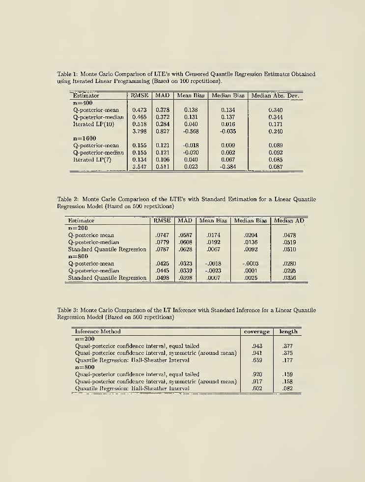
Table 1: Monte Carlo Comparison of LTE's with Censored Quantile Regression Estimates Obtained

using Iterated Linear Programming (Based on 100 repetitions).

Estimator RMSE MAD Mean Bias Median Bias Median Abs. Dev.

n=400Q-posterior-mean 0.473 0.378 0.138 0.134 0.340

Q-posterior-median 0.465 0.372 0.131 0.137 0.344

Iterated LP(10) 0.518 0.284 0.040 0.016 0.171

3.798 0.827 -0.568 -0.035 0.240

n=1600Q-posterior-mean 0.155 0.121 -0.018 0.009 0.089

Q-posterior-median 0.155 0.121 -0.020 0.002 0.092

Iterated LP(7) 0.134 0.106 0.040 0.067 0.085

3.547 0.511 0.023 -0.384 0.087

Table 2: Monte Carlo Comparison of the LTE's with Standard Estimation for a Linear Quantile

Regression Model (Based on 500 repetitions)

Estimator RMSE MAD Mean Bias Median Bias Median ADn=200Q-posterior-mean .0747 .0587 .0174 .0204 .0478

Q-posterior-median .0779 .0608 .0192 .0136 .0519

Standard Quantile Regression .0787 .0628 .0067 .0092 .0510

n=800Q-posterior-mean .0425 .0323 -.0018 -.0003 .0280

Q-posterior-median .0445 .0339 -.0023 .0001 .0295

Standard Quantile Regression .0498 .0398 .0007 .0025 j .0356

Table 3: Monte Carlo Comparison of the LT Inference with Standard Inference for a Linear Quantile

Regression Model (Based on 500 repetitions)

Inference Method coverage length

n=200Quasi-posterior confidence interval, equal tailed .943 .377

Quasi-posterior confidence interval, symmetric (around mean) .941 .375

Quantile Regression: Hall-Sheather Interval .659 .177

n=800Quasi-posterior confidence interval, equal tailed .920 .159

Quasi-posterior confidence interval, symmetric (around mean) .917 .158

Quantile Regression: Hall-Sheather Interval .602 .082

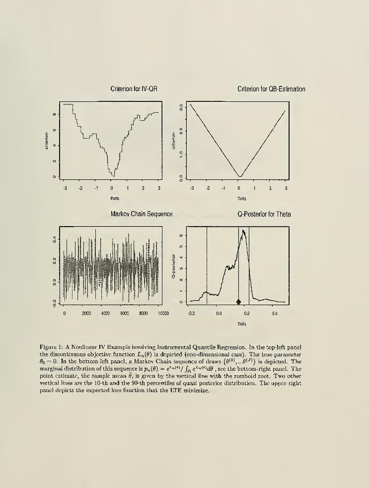
Criterion for IV-QR Criterion for QB-Estimation

Markov Chain Sequence Q-Posterior for Theta

2000 4000 6000 10000 -0.2 0.0 0.2

thela

0.4

Figure 1: A Nonlinear IV Example involving Instrumental Quantile Regression. In the top-left panel

the discontinuous objective function Ln {9) is depicted (one-dimensional case). The true parameter

#o = 0. In the bottom-left panel, a Markov Chain sequence of draws (9^\ ...9<-J^) is depicted. The

marginal distribution of this sequence is pn (9) = e Ln(8) / fQ e L "wd& , seethe bottom-right panel. Thepoint estimate, the sample mean 9, is given by the vertical line with the romboid root. Two other

vertical lines are the 10-th and the 90-th percentiles of quasi-posterior distribution. The upper-right

panel depicts the expected loss function that the LTE minimize.

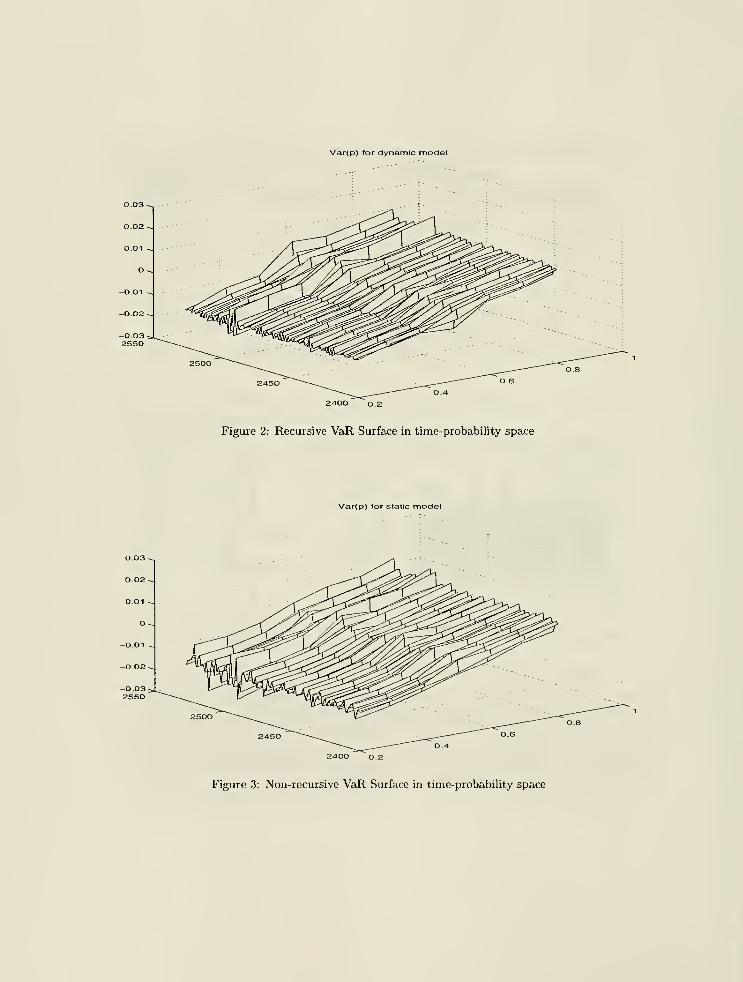
Var(p) for dynamic model

2400 o.2

Figure 2: Recursive VaR Surface in time-probability space

Var(p) for static model

2400 o.2

Figure 3: Non-recursive VaR Surface in time-probability space

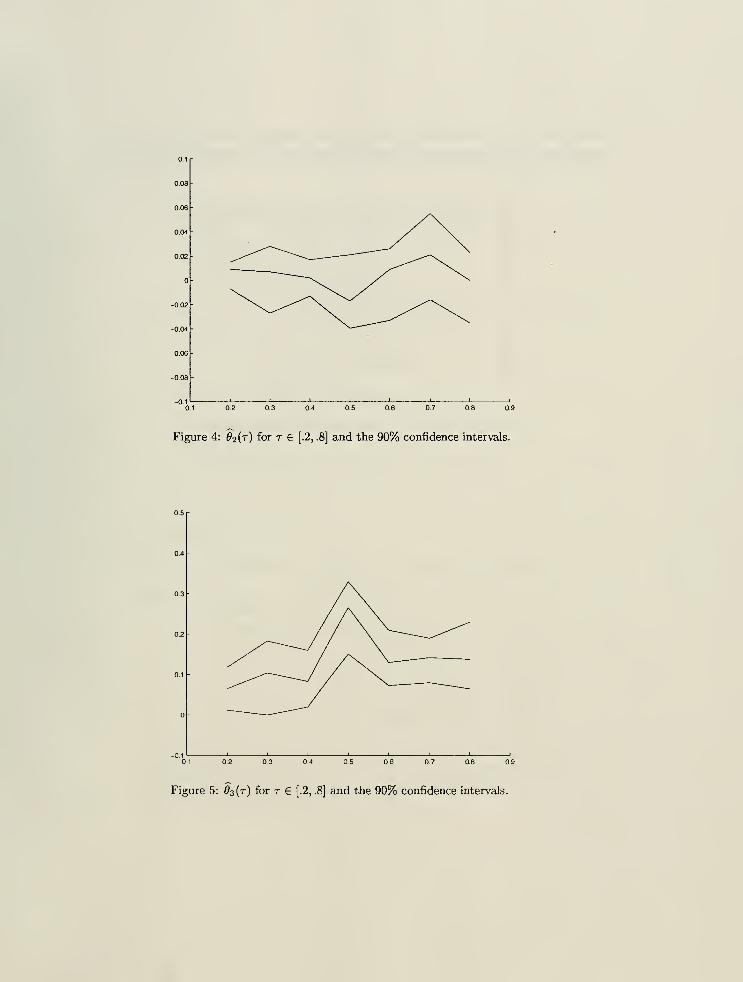
0.2 0.3 0.4 0.5 0.7 0.8

Figure 4: #2(1") for r € [.2, .8] and the 90% confidence intervals.

Figure 5: 0s{t) for t € [.2, .8] and the 90% confidence intervals.

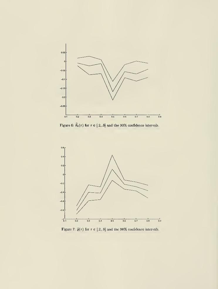
0.1 0.2 0.3 0.4 0.5 0.6 07 0.8 0.9

Figure 6: 9* (t) for r 6 [.2, .8] and the 90% confidence intervals.

0.1 0.2 0.3 04 05 0.6 07 0.8

Figure 7: g(r) for r 6 [-2, .8] and the 90% confidence intervals.

Throughout this proof the range of integration for h is implicitly understood to be Hn . For clarity of the

argument, we limit exposition only to the case where J„(9) and tt„(9) do not depend on n. The more general

case follows similarly.

Part 1. Define

then

h = y/H(9-Tn ), Tn =eo +-J(0o)-' A„(9 ), U„ = -^=J(9 )-' A„(0O ),n y'n

p"n (h) =-y=pn (h/Vn + 9 + U„lVn)

where

and

7r (^ +T") exp(^(7% +T"))

/«„ * (ts + T") exp(L- {7s + T")) dh

7r (^r +T") exp(w(ft))

~fH„*(^+Tn)exp(u(h))dh

7r (v^+T") exp(u'W)

u> (h) = Ln (rn + -j=\ - L (9 ) - i-A„ (9o)' J {9 )-' A„ (9 )

,

C„ = f 7v f-j= + T„) exp (u(h)) dh.

Part 2 shows that for each a > 0,

Am=[ \h\a ey.p(w{h))n(Tn +~\-eKP (-^h'j(9 )h\n(9o

Given (A .4), taking a = we have

C„-> p /" e-i h'

Jieo)hTr(9 )dh = iT(eo)(,2iT)i\<ietJ(9 )\-

i/2,

dh^+0.

hence

Next note

where

C„ = Op (l).

left side of (A. 1) = f \h\a\p'n (h) -p'00 (h)\dh = An C~'

,

„ = /"|fc|

Qeu,('°7r(V,! + -^=) -(27r)-

d/2|detJ(5o)r /2 exP r-^'J(eo)^ C„ dh.

Using (A. 5), to show (A.l) it suffices to show that An —> 0. But

An < A tjl + A2n

(A.2)

(A.3)

(A.4)

(A.5)

29

where

A2n = f \h\a Cn {2-K)-

d,2\AetJ(fio)\

U2 &^{-\h'J{9o)h\ -7r(0o)exp (-\h'J(9 )h\

Then by (A.4)

dh.

and

C„(27r)-d/2

|detJ(e )|1/2

-7r(6lo)| f \h\a exp f-lh'J(9 ) h\ dh

Part 2. It remains only to show (A.4). Given Assumption 4 and definitions in (A. 2) and (A. 3), write

- ^-An (fi)' J (9 )-' A„ (fl ) + i?n f-^: + T„)

= -\tiJ{6o)h + IU f-j= + T„y

Split the integral A\ n in (A.4) over three separate areas:

rea (i) : \h\ <M,

rea (ii) M <\h\< Sy/n,

rea (iii) \h\ > Sy/n.

Each of these areas is implicitly understood to intersect with the range of integration for h, which is H„.

Area (i): We will show that for each < M < oo and each e >

liminfP,•{/[ J\h\<t

\h\< exp(w(h))7z(rn + -^=\

- exp (- hi J (fl ) h\ -k (do) \dh < e \

(A.6)

> 1-e.

This is proved by showing that

exp(w(h))n (t„ + -j=\ - exp (-lh'J(6 )h\ 7r(0o )

Using the definition of ui (h), (A. 7) follows from:

sup \h\°

\h\<M(A.7)

(a) sup|M<M "ts

+T")

7T (0O ) 0, (6) sup\h\<M "•(^ +T") o,

where (a) follows from the continuity of 7r() and because by Assumption 4ii-4.iii:

1

JnJ(8 )-'An (9 )=Op (l). (A.8)

30

Given (A.8), (b) follows from Assumption 4.iv, since

hsup\h\<M

Tn +\pn

Op{\/y/n).

Area (ii): We show that for each e > there exist large M and small 5 > such that

\unmfl\{ I \h\a

|exp (w(h)} it (t„ +

-J=j4/ '-

J_JM<\h\<6Sn

-exp(-*-tiJ{e )h\n{9 ) dh < e \ > 1 -

(A.9)

Since the integral of the second term is finite and can be made arbitrarily small by setting M large, it suffices

to show that for each e > there exist large M and small i5 > such that

liminf P,\ [ \h\" exp(w(h))w [Tn + -^= ) dh < e In [JM<\h\<6^ \ V"/ J

In order to do so, it suffices to show that for sufficiently large M as n —> oo

> 1-e.

By assumption 7r(-) < K, so we can drop it from consideration.

By definition of w{h)

exp (w (h)) < exp[— -h'J (6o) h + Rn ('-*)

Since \T„ — do\ = op (l), for any S > wp —> 1

T„ H r= — 8o•Jn

< 25, for all \h\ < 8^/n.

Thus, by Assumption 4.iv(a) there exists some small <5 and large M such that

liminfPA sup\Rn (Tn + -$=)\ j

< imineig(J(e )) J.>l-e.<|hl<*Vn \h + ^J(6 )- 1 A„ (So)

|

2 ~ 49o))|

Since £|J (e )~ l An (fl ) [

2 = Op (1), for some C >

liminfP.^ exp(u>(/i)) < Cexp(-ift'J(fl )ft

°|e'" c 't) <CexpC-l>liminfpje"' ( 't) < Cexp -±/i'J (9 ) h + ^mineig(J (0O )) |ft|:

> 1-e.

(A. 12) implies (A. 11), which in turn implies (A.9).

(A. 10)

exp(io(ft))7r (T„ + -^=J< Cexp (-ife',7(6>o) ft) , for all M < \h\ < 6y/n. (A.ll)

(A.12)

31

(A.13)

> 1-e.

Area (iii): We will show that for each e > and each S > 0,

liminfPA f \h\a

exp(tu (h)) -k (T„ + -^-)

-expf--/»'j(0o )/i) tt(0o) d/i<el

The integral of the second term clearly goes to as n — oo. Therefore we only need to show

f |fc|ae"

(fc)7r (t„ + -^=) dh^ p 0.

Recalling the definition of h, the term is bounded by

^/nx+i

f T„-e 7r(fl)exp[£n (fl)-i„(9o)-^-A„(9o)'J(flo)-, A„(e

) )d9.J\e-Tn \>s \

2n/

Since T„ — 9o — 0, wp -> 1 this is bounded by

tf„ • C •^+1/ (1 + |0|

Q) 7T (0) exp (L„ (0) - L„ (0O)) <#,

/|9-9 l>S/2

where

tf„ = exp f-ii. (0o )' J (ft,)

-1 An (0O)J

= Op (l).

By Assumption 3 there exists e > such that

liminf P.[ sup e*-m-L.lto) < e

-«l = 1n-+°°

(_|9-9ol>*/2 J

Thus, wp —> 1 the entire term is bounded by

K„C- v^"1" 1

e- "'

/ |(9|°tt (0) d0 = op (l). (A.14)

Here observe that compactness is only used to insure that

/ |0|

Q7r(0)d0<oo. (A. 15)

J&

Hence by replacing compactness with the condition (A. 15), the conclusion (A.14) is not affected for the given

a.

The entire proof is now completed by combining (A.6), (A.9), and (A.13).

A.2 Proof of Theorem 2

For clarity of the argument, we limit exposition only to the case where Jn (0) and ii„(9) do not depend on

n. The more general case follows similarly.

Recall that

h = VM0 - Oo) -J(9o)~l A„ {Oo) iVn.

32

Define Un = J(9o) 'An (0o)/\/n. Consider the objective function

Qn(z)= f p(,z-h-U„)p'„(h)dh,

which is minimized at y/n{9 — do). Also define

Q=»(z) = / p(z-h-U„)pUh)dh.J**

which is minimized at a random vector denoted Zn . Define

l \hi£ = arginf < I p(z - h) p"^{h) dh \

.

z£* d{ Jit*

J

Note that solution is unique and finite by Assumption 2 parts (ii) and (iii) on the loss function p. When p

is symmetric, $ = by Anderson's lemma.

Therefore, Zn — arginfz6RdQoo(z) equals

Z„=Z + Un =Op (l)-

Next, we have for any fixed z

Qn(z) - Qoo(zHp

since by Assumption 2.ii p(h) < 1 + \h\p and by \a + b\" < 2p~ l

\a\p + 2

p_1|b|" for p > 1:

|Q„(Z)-Qco(z)|< / {l + \z-h-Un n\pl(h)-pZo{h)\dh

+ / (l + \z-h-Un\

p)(pUh))dh

< f (l+2p- 1

\h\" + 2"- 1 \z-Un \")\p'n {h)-p'00 (h)\dh

+ [ {l + 2"- ,

\h\p + 2'" , \z-Un

\

p ){p'0O (h))dh

< / (l + 2p- 1

\h\p +Op(V)(p'n(h)- PUh))dh

+ f {l + 2»- 1

\h\p + Op(l))(pUh))dh = op (l) >

where op (l)-conclusion is by Theorem 1 and exponentially small tails of the normal density (Lebesgue

measure of H^ converges to zero)

.

Now note that Qn {z) and Qoo(z) are convex and finite, and Zn = arginf26Rti(5oo(z) = Op {\). By the

convexity lemma of Pollard (1991), pointwise convergence entails the uniform convergence over compact sets

K:

sup \Q„(z) - Qoo(z) ->> 0.

Since Z„ = Op (l), uniform convergence and convexity arguments like those in Jureckova (1977) imply that

\/n{9 — 6o) — Zn -t p 0, as shown below.

Proof of Zn — \/n{Q — 6q) = op {\). The proof follows by extending slightly the convexity argument of

Jureckova (1977) and Pollard (1991) to the present context. Consider a ball Bi(Zn ) with radius 8 > 0,

33

centered at Zn , and let z = Zn + dv, where v is a unit direction vector such that \v\ = 1 and d > S. Because

Zn = Op (l), for any 6 > and e > 0, there exists K > such that

HminfP,{En = {Bs (Zn ) 6 BK {0)}} > 1 - e.

By convexity, for any z = Zn + dv constructed so, it follows that

J(Q«(*)-Q«(Z«)) > Qn(z')-Qn (Zn ),

(A.16)

where z* is a point of boundary of Bg(Z„) on the line connecting z and Z„. By the uniform convergence of

Qn(z) to Qoo(z) over any compact set Bk(0), whenever E„ occurs:

^(<9n(z) - 0„(Z»)) > Q„(**) - Q»(Z„)

> Qoo(z*) - Qoa(Z„) +Op(l) > V„ + Op(l),

where V„ > is a uniformly in n positive variable, because Z„ is the unique optimizer of Qoo- That is, there

exists an 7j > such that lim inf„ P(Vn > rj) > 1 — e. Hence we have with probability at least as big as

1 — 3e for large n:

2(Qn(z)-Q„(zn))> v.

Thus, y/n(8 — 0q) eventually belongs to a complement of Bg(Z„) with probability at most 3e. Since we can

set e as small as we like by picking (a) sufficiently large K, and (b) sufficiently large n, and (c) sufficiently

small r\ > 0, it follows that

limsupP'{|Z„ -x/ra(0-0o )| > s] = 0.

Since this is true for any 8 > 0, it follows that

Z„ -Vn(e-6 ) = op (l). U

A.3 Proof of Theorem 3

For clarity of the argument, we limit exposition only to the case where J„(9) and f2n (0) do not depend on

n. The more general case follows similarly. We defined

*i,»(aO = f pn (6)d6.eee:g(e)<

Evaluate it at x = g(0o) + s/yjn and change the variable of integration

Hg ,n(s) = Fg ,n (g(9o) + s/y/n) = f p"„(h)dh.

Hs ,n(s) = / P'x (h)dhJ/i6R J

: 9 (9 +fc/ vAf+t/„/VH')<9(9o)+s/v/:S

H9 ,oo(s) = I plcitydh.

34

By definition of total variation of moments norm and Theorem 1

sup \Hg>n (s) - Hg ,n (s)\-yp 0,

where the sup is taken over the support of Hgi„(s).

By the uniform continuity of the integral of the normal density with respect to the boundary of integration

sup|-ffs ,„(s) - Hgtao (s)\->p 0,

which implies

SUp \Hg,n (s) - Hg i00 (s)\-*p 0.

3

where the sup is taken over the support of Hg<n (s).

The convergence of distribution function implies the convergence of quantiles at continuity points of distri-

bution functions, see e.g. Billingsley (1994), so

H-Ua) - H~Ua)^P 0.

Next observe

ffs,»(s) = p{Vg(0o)'tf(Un , J-,

(0o)) < s\un ],

H'Ua) = Vg{8 )'Un + qa ^V<,g{e )'J-i(6 )Veg(e ),

where qa is the a-quantile of A/"(0, 1).

Recalling that we defined cg ,„(a) = F~l(a), by quantile equivariance with respect to the monotone trans-

formations

Hg ,i(a) = Vn (cj,„(a) - g(8 ))

so that

%Mc9,n(a) -ff(0o)) = Vg{eo)'Un +qa ^s9{Soyj- 1 (e )Veg(.e ) + op (l).

The rest of the result follows by the A-method.

A.4 Proof of Theorem 4

In view of Assumption 4, it suffices to show that

J;'W-^'(«oK0, (A.17)

and then conclude by the A-method.

Recall that

h = V^(o - e )- j„ (flo)

-1a„ (0O ) M^,

' - '

and the localized Quasi-posterior density for h is

p*„ (h) = —=pn (h/y/n + 9o + Un/y/n) .

y/Tl

35

Note also

J-\e )= f n{8 - ff){6 - 9)'pn (9)d9

= f (ft - JH{9- 9 ) + U„) (h - yft{8-8o) + Un )'p'„(h)dh,

and

J-1

{9 )= f htiplcWdh.

We have, denoting h = (hu ...,dd ) and fn = (T„i, ...,Tnd ) where f„ = V"(0 - 0o) - t/„, for all i,j <d

(a) /Hn fchj (p'n (h) - pUh))dh = op (l) by Theorem 1,

(b) JHC hihj lp^(h))dh = op (l) by definition of p*x and J„(6o) being uniformly nonsingular,

W /*„ l^"|2

(p"n(h)-pUhj)dh = op {l) by Theorem 2,

(d) /H |Tn|2

(ptcC1))^ = °p(1) by Theorem 2, definition of p'^, and J„(0o) being nonsingular,

{e) fH^hj fni (p*„(h) -p*00 (h))dh = ov (1) by Theorems 1 and 2,

=<v(i>

(f) JH hj T„i (p^oW)*"1 = °p(l) by Theorems 1 and 2, definition of p^,, and J„(#o) being uniformly

=Op(l)

nonsingular, from which the required conclusion follows.

A.5 Proof of Proposition 1

Assumption 3 is directly implied by (4.1)-(4.4) and the uniform continuity of Ew.i (ff), as shown in Lemma

1. It remains only to verify Assumption 4.

Define the identity

L„(9) - L„(9 ) = - ngn (9o)'W(6 )G(9 )(6 - )

A„(» )'

(A.18)

-H<,e-0Q)'nG(0o)'W{9o)G{0o){8-0o ) + Rn(9).Z ^

^*

Next, given the definition of A„(#o) and J{9o), conditions i, ii, iii of Assumption 4. are immediate from

conditions i-iii of Proposition 1. Condition iv is verified as follows. Condition iv of Assumption 4 can be

succinctly stated as:

./ \R„ (9)|

1

\ |9-"

o|<*l + n|0-0o| 2

J

for each e > there exists a 5 > such that lim sup P* < sup r-—-—tj > e > < e

36

This stochastic equicontinuity condition is equivalent to the following stochastic equicontinuity condition,

see e.g. Andrews (1994a):

forany5„->0 sup _£=ML_ = 0p (l). (A.19)W-9o\<t~ l+n\(f—(fo\

This is weaker than condition (v) of Theorem 7.1 in Newey and McFadden (1994), which requires

SUP -f=Ta a i . m H~ll = »W > (A - 20)

Rn (0) Rn (6) ^/ii\9 - 6p\ + n\B - 6p

l+n|0-0o|

2

21

l + n|0-0o| 2 ^/E\9 - 9\+ n\9 - 9o\

2

where the term in brackets is bounded by

y/E\9-9\

^ l + n\9-9\

2 ~ '

Hence the arguments of the proof, except for several important differences, follow those of Theorem 7.2 in

Newey and McFadden (1994).

At first note that condition iv of Proposition 1 is implied by the condition (where we let g (9) = Eg„ (9)):

sup e (9) = op f-L)

, where e (0) = g"<2f

3"^

o) ~f

(<?)for any ft. -* 0. (A.21)

esBj„(e ) Vv"/ l + -/n|0-0o|

From (A.18)

Rn {9) = Rln(9) + R2n(6) + R3n(9),

where

Rln (9) =n(gn (0O )'Wn {9)G (9 ) (9 -9 ) + \(9- 9 )' G (9 )' W{B)G{9 ) (9 - 9 )

- \9n (9)' Wn (9)gn (9) + \gn (0O)' Wn (9)gn (0O))

,

R2„ (9) =n(^gn (9o)' (Wn (9 ) - Wn (0)) gn (0O)Y

R3n (9) =n (gn (fio)' (W(9 )- Wn (9))) G (0o) (9 - 0o)

+ \(9- Bo)' G (fl )' (W{9 ) - W{9)) G (9 ) (9 - O))

Verification of (A. 19) for the terms R2n {9) and R3n immediately follows from ,/ngn (9o) = Op (l) and the

uniform consistency ofWn (9) in 9 as assumed in condition i of Proposition 1 and from the continuity ofW (9)

in 9 by condition i of Proposition 1, so that Wn (9) - W{9) = op (l) uniformly in 9 and W{9) - W(9 ) = o(l)

as \9 - O |

-> 0.

It remains to check condition (A. 19) for the term Ri n (0). Note that

gn (0) = (1 + v/S|0 - 0o|) e (0) + g (0) + gn (0O ) .

37

Substitute this into R\ n (9) and decompose

- -flm («) = I (1 + v^|0 - 0o|)2e (0)' W„(9) e (0) + S„ (to)' Wn(0)(9 (<?) - G (9 )) (9 - 9

)n 2__ ' , » v '

+ (i + V^\e - e\) « (0)' w„(%» (fl ) + (i + V£|0 - to|) <= (e)' vk„(% (e)

> „ ' >,

'

+ \g (<?)' (w.W - w(*)) 9 (0) + ^<? (0)' w(9)9 (e) -l-{e-e )'G (e y w(B)G (e

) (e - o ).

xw

/ X w*

r5 (9) r6 (9)

Using the inequalities, for x > 0:

(1 + ^/m:)2

< 2yfnx < J

1 + y/nx< g

n (1 + Vnx) < 2Vn (A. 22)

1 + Til2_

' 1 + ra! _' 1 + rtx2 ~ ' 1 + nx2 ~~ x

'

each of these terms can be dealt with separately, by applying the conditions i- iii and (A.21):

<a > supi j?

1

?//^ 12 ^ SUP «eWW.(ff)e(tf)=«y(l)>

m «|r2 (fl)|

o(VH|0-0o|)' ,m ,- -„ . m(6)

SUPt ,

i fl a i2= SUP ,1 o—JiT^"Wv"»» (to) = oP (1)

,

ees^ («o) * + n\

e ~ e°\ 96B,„ (» ) 1 + n|0 - O|

2

M supi a"

1

?/^ i2 ^ sup 2«l«(0)'w«(0)0»(to)l = °i.(i),

(<*) sup! ."LV/^ |2

< ^p 2^ e(0)'Wn (0)-9-^-So|

= 0,(1),

±i (g) I < supIffWI

2

w sup , , :.v 1,2 < -p iSViw-(«)-^(»)i = ^(i).

m n|rg(g)j o(|6>-go|2lV^(g)|) ...

(/) SUPi + '

ifl a 12 ^ SUP| fl fl |2

= °p t1) •

where (a) follows from (A.22), (A.21), and condition i, which states that Wn {9) = W{9) + op (l) and

W{9) > is finite uniformly in 9; in (b) the first equality follows by Taylor expansion g(9) — G (9o) (9 — So) +o{\9 — 9o\) and the second conclusion follows from (A.22) and condition iii; (c) follows from (A.22), (A.21),

condition i and iii; (d) follows by (A.22) and then replacing, by condition ii, g{9) with G (9o) (9 — 9o) +o{\9 — 9q\), followed by applying (A.21) and condition i; (e) follows from replacing by condition ii g(9)

with G (9o) {9 — 9a) +o(\9 — 9o\), followed by applying condition i; and (f) follows from replacing g (9) with

G (9o) (9 - 9o) + o (\9 — 9o\), followed by applying condition i.

Verification of (A. 20) for the term R]„{0) now follows by putting these terms together.

A.6 Proof of Proposition 2

Verification of Assumption 3 is standard given the stated conditions and is subsumed as a step in the

consistency proofs of extremum estimators based on GEL in Kitamura and Stutzer (1997) for cases when s

is finite and Kitamura (1997) for cases when s takes on infinite values. We shall not repeat it here. Next,

38

we will verify Assumption 4. Define

7(0)=arg inf Ln (9,y).

It will suffice to show that uniformly in 9n 6 Bs„(9o) for any <5„ —> 0, we have the GMM set-up:

! » \ (A.23)

-K^!> (0*)) (V^oJ + oj.a))-1 f-^f^nn^Jj,

where

V(9 ) = Errn {6 ) rm (0O)' -

The Assumptions 4.i-iii follow immediately from the conditions of Proposition 2, and Assumption 4.iv is

verified exactly as in the proof of Proposition 1, given the reduction to the GMM case. Indeed, defining

g„(9) = i127=1 mi(Q)i tne Donsker property assumed in condition iv implies that for any e > 0, there is

5 > such that

HmsupPV sup Vn\gn(8) - gn {8o) - (Egn (9) - Egn (6 ))\ > e\ < e,

which implies

limsupP'I sup^\9^)-9n{9o)-(Egn(9)-E9n (9o))\ > 1 <£

n-njo [ffgBstSo) 1 + y/n\9 — 9o\ I

which is condition iv in Proposition 1. The rest of the arguments follow that in the proof of Proposition 1.

It only remains to show the requisite expansion (A.23). We first show that

W»)-*j. o.

For that purpose we use the convexity lemma, which was obtained by C. Geyer, and can be found in Knight

(1999).

Convexity Lemma. Suppose Qn is a sequence of lower-semi-continuous convex R-valued random functions,

defined onRd , and let V be a countable dense subset ofR1*. If Q„ weakly converges to Q^, in R marginally (in

finite-dimensional sense) on V where Qoo is lower-semi-continuous convex and finite on an open non-empty

set a.s., then

arginf Q„{z)-y d arginf Qoo(z),zeR d z£R d

provided the latter is uniquely defined a.s. in3d

Next, we show that 7(0„)->p 0. Define F = {7 : Es{mi{9 )'j\ < 00} and Fc = {7 : Es[mi(9oY"f] = 00}.

By convexity and lower-semicontinuity of s, F is convex, open, and its boundary is nowhere dense in Rp.

Thus for 7 e F, Es[mi(8)'^] < 00 for all 9 e Bg(9o) and some 6 > 0, which follows by continuity of

9 i-+ Es[mi(9)'^/] over B{(9o) implied by the condition ii and iii.

Thus, for a given 7 e F and any 9n —> p 9a

-^s[tti,(6>„)'7Hp Es[mi(9o)'H < 00.

39

This follows from the uniform law of large numbers implied by

1. {s[mi(8)'f],9 6 B&(9o)}, where S is sufficiently small, being a Donsker class wp — 1, and

2. Erriiifi) — J x dP[mi(8) < x] being continuously differentiable in 9 by condition ii and iii.

The above function set is Donsker by

(a) mi(6)'-y € M for some compact M and a given 7 e F, by condition iii,

(b) {jrii(8),9 e Bg(8o)} being Donsker class by condition iv,

(c) s being a uniform Lipschitz function over V D M 1T, by assumption on s,

(d) mi(<?)'7 e V for all 6 € Bs(9o), some 5 > 0, and a given 7 £ F, by construction of F,

(e) Theorem 2.10.6 in van der Vaart and Wellner (1996) that says a uniform Lipschitz transform of a

Donsker class is Donsker class itself.

Now take 7 in Fc\ dF, where dF denotes the boundary of F. Then wp —> 1

1 ^—>J s[mi(6„)'-y] = oo-fp Es[m.i{8o)'"i] = 00.

Now take all the rational numbers 7 6 Rp\ dF as the set T> appearing in the statement of the Convexity

Lemma and conclude that

7(0nH P = arg inf7£s[mi(0o)'7].

Given this result, we can expand the first order condition for 7(#„) in order to obtain the expression for its

form. Note first

n

= Yl Vs (7(0*)' mi (0«)) ™i (9")

•':'(A.24)

t=i

where1 "

V„ = -^V 2s(7(fl„)'m,(e„))mi (9„)Tn i (9T,)',

i = l

for some ~t{8n) between and 7 (9n ), which is different from row to row of the matrix V„.

Then

K.->p V{0o) = Errn (9 ) rm (9 )'

This follows from the uniform law of large numbers implied by

1. {V 2s(-y'mi(9'))mi(9)mi(8)' ,(9',-y,9) e Bs^(9 ) x Bj2 (0) x Bs3 (9 )}, where Sj > are sufficiently

small, being a Donsker class wp — 1,

2. Emi(9)mi{9)' = J xx'dP[m.i(8) < x] being continuous function in 9 by condition i,

17Recall that V is defined as the open convex set on which s is finite.

40

3. EV 2s{~f'mi (0*))m,- (£>) rm (9)' = EV2

s{0)rrii [9) m; (0)' + o(l) uniformly in (9, 9") 6 Bj(5 ) x B*(0O ) for

i

sufficiently smaJl S > 0, for ajiy 7 — 0, by assumptions on s and condition iii.

The claim 1 is verified by applying exactly the same logic as in the previously stated steps (a)-(e). For the

sake of brevity, this will not be repeated.

Therefore, wp — 1

7(fl») = -(Vrn)

-1 -y)mI-(flB ) = -(V(tfor1 +Op(l))-X)mi (flB ). (A.25)

ft . n .

t=i t=i

Consider the second order expansion,

1 " 1

M0„,7(0„))=-v/S7(0n)'-7=y>< (0n)+ rV^7(0„)'V„v^7(0«)> (A.26)

where

for some 7 (#„) between and 7 (#n ), which is different from row to row of the matrix V„. By a preceding

argument,

V;-> P V(9 ).

Inserting (A.25) and V„ = V(9o) + op (l) into (A.26), we obtain the required expansion (A.23).

A.7 Proof of Proposition 3

Assumption 3 is assumed. We need to verify Assumption 4.

Define the identity

Ln (9) - Ln (9 ) = £m,-(0o)'(0 - 9 )

A»(»o)'

+ \<fi- 9o)'nVee.Emi(eo)(9-9 )

(A.27)

-JWo)

+ Rn{9).

Assumption 4.i-iii then follows immediately from conditions i and ii. Assumption 4.iv is verified as follows.

The remainder term Rn (9) is given the following decomposition:

R„ (9) = ]T {mi(9) - m,(0o ) - £m,(0) + Emi{9 ) - m,{9 )'{9 - 9 )j

+ n (Em,(9) - £m,(0o )) + \{9 - 9 )'nJ{9 ){9 - 9 )

.

41

It suffices to verify Assumption 4.iv separately for Ri„(9) and R2n{9). Since

R*n(0) = -|n(0 - Bo)' \J{9') - J(9 )] (9 - 9 ),

for some 9' on the line connecting 9 and 9o, verification of Assumption 4 for R2n (9) follows immediately

from continuity of J(9) in over a ball at 9o-

To show Assumption 4.iv-(b) for Ri„(9), we note that for any given M >

limsupP'i sup l-Ri* (0) |> e I

B |_|9-8 |<M/ V/S' J

<limsuP pl sup ifl-flol1^'"^, 1 >e\ (A.28)

n ^|9-e |<M/VH' |f - »0|J

<HmsuPp( sup ^JgLLMl >e}=0

,

where the last conclusion follows from two observations.

First, note that

7 lf>\ = Rl» W - J_V (mW ~ m'(g°) ~ (

EmiW ~ ErmW) ~ rni{9 )'{9 - fl) \nW ~ y/E\e-0O

\ V^fcfV |*-flo| /

is Donkser by assumption, that is it converges in t°°(Bg(9o)) to a tight Gaussian process Z.

The process has uniformly continuous paths with respect to the semimetric p given by

p2(9 1 ,92 ) = E(Z(9 1 )-Z(92 ))

2,

so that p(9,9) —> if 9 — 9o- Thus almost all sample paths of Z are continuous at So-

Second, since by assumption

E[mn (9) - m„(9 ) -l*Z{9o)'{9 - 9 )f = o{\9 - <?|

2

),

we have for any 9n — 9o

E*

therefore

i/<Y,aU! f_°(|0n-0|2

) _Qj

,V^|Cn -Sol. |»n - 0O|2

z(e ) = o.

Therefore for any 6'—

¥

v 9o, we have by the extended continuous mapping theorem

ZniP')-*d Z(9 ) = 0, that is Zn (9')-* p 0. (A. 29)

This shows (A.28).

To prove Assumption 4iv-(a) for R\ n (9), we need to show that for some 5 > and constant M

i"'— !>/'[

sup 'f.'"^! >e\<e. (A.30)

42

Using that M/y/n < \9 — 9o\, bound the left-hand-side by

,. p . f |-Rln(0)| 1 \Iim sup P < sup ' ,, —7=7- — > e >

\M/.fR<\e-e \<5 Vn\9-9 \y/n\9-8

\ J

< hm sup P < sup -ipr-—-i-• 77 > e >

<limsupP*{ sup |Zn (0)|.J_> e L

" ^M/ v'S'<|e-«ol<* !

(A.31)

where for any given e > in order to make the last inequality true, we can make either S sufficiently small

by the property (A. 29) of Zn or make M sufficiently large by the property Zn = Op- (1).

B Appendix on Computation

B.l A computational lemma

In this section we record some formal results on MCMC computation of the quasi-posterior quantities.

LEMMA 3 Suppose the chain (9 ,j < B) is produced by the Metropolis Hastings(MH) algorithm with q

such that q{8\8') > for each (9,9'). Suppose also that P{p(9U) ,£) = 1} > for all j > i - Then

1. Pn(-) is the stationary density 0} the chain,

2. the chain is ergodic with the limit marginal distribution given by pn ():

B

where the supremum is taken over the Borel sets,

3. For any pn - integrable function g:

D

lim sup \p(9iB) e A\9 )

- f Pn<fi)do\ = 0,»->oo A I Ja

1

Br

Y^g(9b))^P / g(9)pn (9)d9.

Proof. The result is immediate from Theorem 6.2.5 in Robert and Casella (1999).

An immediate consequence of this lemma is the following result.

LEMMA 4 Suppose Assumptions 1 and 2 hold. Suppose the chain {9(-'\j < B) satisfies the conditions of

Lemma 3, then for any convex and pn -integrable loss function p„ (•)

are infS£0

provided that 9 is uniquely defined.

1

B1 r

/•

i^p„(e (j'-0) ->„0 = argmf / p„(8 - 9)pn {9)d9

43

Proof. By Lemma 3 we have the pointwise convergence of the objective function: for any 9

B

>0)dO,

which implies the result by the Convexity Lemma, since 6 i-> J pn {9 — 9)pn (9)d9 is convex by convexity of

pn -

B.2 Quasi-Bayes Estimation and Simulated Annealing

The relation between drawing from the shape of a likelihood surface and optimizing to find the mode of the

likelihood function is well known. It is well established that, e.g. Robert and Casella (1999),

Km f u „, ,„/,„ = argmaxXn (0) (B.l)A-xx. /e exz-(9)7r(5)d9 »e9

Essentially, as A — oo, the sequence of probability measures

eXL^eK(9)

converges to the generalized Dirac probability measure concentrated at argmax L„ (9).

(B.2)

The difficulty of nonlinear optimization has been an important issue in econometrics (Berndt et al. (1974),

Sims (1999)). The simulated annealing algorithm (see e.g. Press et al. (1992), Goffe et al. (1994)) is usually

considered a generic optimization method. It is an implementation of the simulation based optimization (B.l)

with a uniform prior n (9) = c on the parameter space 0. At each temperature level 1/A, the simulated

annealing routine uses a large number of Metropolis-Hastings steps to draw from the quasi distribution

(B.2). The temperature parameter is then decreased slowly while the Metropolis steps are repeated, until

convergence criteria for the optimum are achieved.

Interestingly, the simulated annealing algorithm has been widely used in optimization of non-likelihood-based

semiparametric objective functions. In principle, if the temperature parameter is decreased at an arbitrarily

slow rate (that depends on the criterion function), simulated annealing can find the global optimum of

non-smooth objective functions that may have many local extrema. Controlling the temperature reduction

parameter is a very delicate matter and is certainly crucial to the performance of the algorithm with highly

nonsmooth objective functions. On the other hand, as Theorems 1 and 2 apply equally to (B.2), the

results of this paper show that we may fix the temperature parameter 1/A at a positive constant and then

compute the quasi-posterior medians or means for (B.2) using Metropolis steps. These estimates can be

used in place of the exact maximum. They are consistent and asymptotically normal, and possess the same

limiting distribution as the exact maximum. The interpretation of the simulated annealing algorithm as an

implementation of (B.2) also suggests that for some problems with special structures, other MCMC methods,

such as the Gibbs sampler, may be used to replace the Metropolis-Hasting step in the simulated annealing

algorithm.

B.3 Details of Computation in Monte-Carlo Examples

The parameter space is taken to be Q = [8o ± 10]. The transition kernel is a Normal density, and flat

prior is truncated to 0. Each parameter is updated via a Gibbs-Metropolis procedure, which modifies

44

slightly the basic Metropolis-Hastings algorithm: for k = 1, -~,d, a draw of fit from the univariate normal

density q{\(,k — 0Jt \,<t>) is made, then the candidate value £ consisting of £k and 9_^ replaces 0"' with

probability p(6^,£) specified in the text. Variance parameter (/> is adjusted every 100 draws (in the second

simulation example and empirical example) or 200 draws (in the first simulation example) so that the

rejection probability is roughly 50%.

The first N x d draws (the burn-in stage) are discarded, and the remaining N x d draws are used in

computation of estimates and intervals. The starting value is the OLS estimate in all examples. We use

TV = 5, 000 in the second simulation example and empirical example and N = 10, 000 in the second simulation

example. To give an idea of computational expense, computing one set of estimates takes 20-40 seconds

depending on the example. All of the codes that we used to produce figures, simulation, and empirical

results are available from the authors.

Notation and Terms

-tp convergence in (outer) probability P"

—>d convergence in distribution under P'

wp —> 1 with inner probability P» converging to one

~ asymptotic equivalence denoted A ~ B means lim AB~' = I

Bs(x) ball centered at x of radius S >J identity matrix

A > A is positive definite when A is matrix

AT(0, a) normal random vector with mean and variance matrix a

T Donsker class here this means that empirical process / i-> -t= X)™=1 (/(W,-) — Ef(Wi)) is

asymptotically Gaussian in £°°(^r), see van der Vaart (1999)

t°°(J-) metric space of bounded over T functions, see van der Vaart (1999)

mineig(A) minimum eigenvalue of matrix A

References

Abadie, A., 1995. Changes in Spanish labor income structure during the 1980s: a quantile regression approach, CEMFIWorking Paper.

Amemiya, T., 1977. The maximum likelihood and the nonlinear three-stage least squares estimator in the general

nonlinear simultaneous equation model. Econometrica 45 (4), 955-968.

Amemiya, T., 1985. Advanced Econometrics. Harvard University Press.

Anderson, T. W., 1955. The integral of a symmetric unimodal function over a symmetric convex set and some

probability inequalities. Proc. Amer. Math. Soc. 6, 170-176.

Andrews, D. W. K., 1994a. Empirical process methods in econometrics. In: Engle, R., McFadden, D. (Eds.), Handbook

of Econometrics, Vol. 4. North Holland, pp. 2248-2292.

Andrews, D. W. K., 1994b. The large sample correspondence between classical hypothesis tests and Bayesian posterior

odds tests. Econometrica 62 (5), 1207-1232.

Andrews, D. W. K., 1997. A stopping rule for the computation of generalized method of moments estimators. Econo-

metrica 65 (4), 913-931.

45

Andrews, D. W. K., 1999. Estimation when a parameter is on a boundary. Econometrica 66, 1341-83.

Berger, J. O., 2002. Bayesian analysis: a look at today and thoughts of tomorrow. In: Statistics in the 21st Century.

Chapman and Hall, New York, pp. 275-290.

Bemdt, E., Hall, B., Hall, R., Hausman, J., 1974. Estimation and inference in nonlinear structural models. Annals of

Economic and Social Measurement 3 (4), 653-665.

Bernstein, S., 1917. Theory of Probability. (Russian) Fourth Edition (1946) Gostekhizdat, Moscow-Leningrad.

Berry, S., Levinsohn, J., Pakes, A., July 1995. Automobile prices in market equilibrium. Econometrica 63, 841-890.

Bickel, P. J., Yahav, J. A., 1969. Some contributions to the asymptotic theory of Bayes solutions. Z. Wahrsch. Verw.

Geb 11, 257-276.

Billingsley, P., 1994. Probability and Measure, 3rd Ed. John Wiley and Sons.

Buchinsky, M., 1991. Theory of and practice of quantile regression, Ph.D. dissertation, Department of Economics

Harvard University.

Buchinsky, M., Hahn, J., 1998. An alternative estimator for the censored regression model. Econometrica 66, 653-671.

Bunke, O., Milhaud, X., 1998. Asymptotic behavior of Bayes estimates under possibly incorrect models. The Annals

of Statistics 26 (2), 617-644.

Chamberlain, G., Imbens, G., 1997. Nonparametric appliations of Bayesian inference, NBER Working Paper.

Chernozhukov, V., Hansen, C, 2001. An IV model of quantile treatment effects, MIT Department of Economics

Working Paper.

Chernozhukov, V., Umantsev, L., 2001. Conditional value-at-risk: Aspects of modeling and estimation. Empirical

Economics 26, 271-92.

Chib, S., 2001. Markov chain monte carlo methods: Computation and inference. In: J.J.Heckman, Learner, E. (Eds.),

Handbook of Econometrics, Vol 5, Chapter 5. North Holland, pp. 3564-3634.

Christoffersen , P., Hahn, J., Inoue, A., 1999. Testing, comparing and combining value at risk measures, working Paper,

Wharton School University of Pennsylvania.

Diaconis, P., Freedman, D., 1986. On the consistency of Bayes estimates. Annals of Statistics 14, 1-26.

Doksum, K. A., Lo, A. Y., 1990. Consistent and robust Bayes procedures for location based on partial information.

Ann. Statist. 18 (1), 443-453.

Engle, R., Manganelli, S., 2001. Caviar: Conditional value at risk by regression quantiles, Working Paper, Department

of Economics UC San Diego.

Fitzenberger, B., 1997. A guide to censored quantile regressions. In: Robust inference, Handbook of Statistics. Vol. 14.

North-Holland, Amsterdam, pp. 405-437.

Gallant, A. R., White, H., 1988. A Unified Theory of Estimation and Inference for Nonlinear Dynamic Models. Oxford:

Bail Blackwell.

Geweke, J., Keane, M., 2001. Computationally intensive methods for integration in econometrics. In: J.J.Heckman,

Learner, E. (Eds.), Handbook of Econometrics, Vol 5, Chapter 5. North Holland, pp. 3465-3564.

Goffe, W. L., Ferrier, G. D., Rogers, J., 1994. Global optimization of statistical functions with simulated annealing.

Journal of Econometrics 60, 65-99.

46

Hahn, J., 1997. Bayesian bootstrap of the quantile regression estimator: a large sample study. Internat. Econom. Rev.

38 (4), 795-808.

Hansen, L., Heaton, J., Yaron, A., 1996. Finite-sample properties of some alternative GMM estimators. Journal of

Business and Economic Statistics 14, 262-280.

Hansen, L. P., 1982. Large sample properties of generalized method of moments estimators. Econometrica 50 (4),

1029-1054.

Hogg, R. V., 1975. Estimates of percentile regression lines using salary data. Journal of American Statistical Associ-

ation 70, 56-59.

Huber, P. J., 1973. Robust regression: Asymptotics, conjectures, and monte carlo. Annals of Statistics 1, 799-821.

Ibragimov, I., Has'minskii, R., 1981. Statistical Estimation: Asymptotic Theory. Springer Verlag.

Imbens, G-, 1997. One-step estimators for over-identified generalized method of moments models. Rev. Econom. Stud.

64 (3), 359-383.

Imbens, G., Spady, R., Johnson, P., 1998. Information theoretic approaches to inference in moment condition models.

Econometrica 66, 333-357.

Jureckova, J., 1977. Asymptotic relations of M-estimators and R-estimators in linear regression models. Annals of

Statistics 5, 464-472.

Khan, S., Powell, J. L., 2001. Two step estimation of semiparametric censored regression models. Journal of Econo-

metrics 103, 73-110.

Kim, J.-Y., 1998. Large sample properties of posterior densities, Bayesian information criterion and the likelihood

principle in nonstationary time series models. Econometrica 66 (2), 359-380.

Kim, J.-Y., 2002. Limited information likelihood and Bayesian analysis. Journal of Econometrics , 175-193.

Kitamura, Y., 1997. Empirical likelihood methods with weakly dependent processes. Ann. Statist. 25 (5), 2084-2102.

Kitamura, Y., Stutzer, M., 1997. An information-theoretic alternative to generalized method of moments estimation.

Econometrica 65, 861-874.

Knight, K., 1999. Epi-convergence and stochastic equisemicontinuity, Working Paper, Department of Statistics Uni-

versity of Toronto.

Koenker, R., 1994. Confidence intevals for quantile regression. In: Proceedings of the 5th Prague Symposium on

Asymptotic Statistics. Heidelberg: Physica-Verlag, pp. 10-20.

Koenker, R., 1998. Treating the treated, varieties of causal analysis, Lecture Note, Depratment ofEconomics University

of Illinois.

Koenker, R., Bassett, G. S., 1978. Regression quantiles. Econometrica 46, 33-50.

Kottas, A., Gelfand, A., 2001. Bayesian semiparametric median regression modeling. Journal of the American Statis-

tical Association 96, 1458-1468.

Lehmann, E., Casella, G., 1998. Theory of Point Estimation. Springer.

Macurdy, T., Timmins, C., 2001. Bounding the influence of attrition on the intertemporal wage variation in the NLSY,

Working Paper, Department of Economics Yale University.

47

Mood, A. M., 1950. Introduction to the Theory of Statistics. McGraw-Hill Book Company, Inc.

Newey, W. K., 1991. Uniform convergence in probability and stochastic equicontinuity. Econometrica 59 (4), 1161-

1167.

Newey, W. K., McFadden, D., 1994. Large sample estimation and hypothesis testing. In: Engle, R., McFadden, D.

(Eds.), Handbook of Econometrics, Vol. 4. North Holland, pp. 2113-2241.

Newey, W. K., Powell, J. L., 1990. Efficient estimation of linear and type I censored regression models under conditional

quantile restrictions. Econometric Theory 6, 295-317.

Newey, W. K., Smith, R., 2001. Higher order properties of GMM and generalized empirical likeliood estimators,

Working Paper, Department of Economics MIT.

Newey, W. K., West, K. D., 1987. A simple, positive semidefinite, heteroskedasticity and autocorrelation consistent

covariance matrix. Econometrica 55 (3), 703-708.

Owen, A., 1989. Empirical likelihood ratio confidence regions. In: Proceedings of the 47th Session of the International

Statistical Institute, Book 3 (Paris, 1989). Vol. 53. pp. 373-393.

Owen, A., 1990. Empirical likelihood ratio confidence regions. Ann. Statist. 18 (1), 90-120.

Owen, A., 1991. Empirical likelihood for linear models. Ann. Statist. 19 (4), 1725-1747.

Owen, A., 2001. Empirical Likelihood. Chapman and Hall/CRC.

Pakes, A., Pollard, D., 1989. Simulation and the asymptotics of optimization estimators. Econometrica 57 (5), 1027-

1057.

Phillips, P. C. B., Ploberger, W., 1996. An asymptotic theory of Bayesian inference for time series. Econometrica

64 (2), 381-412.

Pollard, D., 1991. Asymptotics for least absolute deviation regression estimator. Econometric Theory 7, 186-199.

Potscher, B. M., Prucha, I. R., 1997. Dynamic Nonlinear Econometric Models. Springer-Verlag, Berlin.

Powell, J. L., 1984. Least absolute deviations estimation for the censored regression model. Journal of Econometrics

, 303-325.

Press, W., Teukolsky, S. A., Vettering, W., Flannery, B., 1992. Numerical Recipes in C, The Art of Scientific Com-

puting. Cambridge.

Qin, J., Lawless, J., 1994. Empirical likelihood and general estimating equations. Annals of Statistics 22, 300-325.

Robert, C. P., Casella, G., 1999. Monte Carlo Statistical Methods. Springer.

Rousseeuw, P. J., Hubert, M., 1999. Regression depth. J. Amer. Statist. Assoc. 94 (446), 388-433.

Sims, C, 1999. Adaptive Metropolis-Hastings, or monte carlo kernel estimation, Working Paper, Department of

Economics Princeton University.

Stigler, S. M., 1975. Studies in the history of probability and statistics. XXXIV. Napoleonic statistics: the work of

Laplace. Biometrika 62 (2), 503-517.

van Aelst, S., Rousseeuw, P. J., Hubert, M., Struyf, A., 2002. The deepest regression method. J. Multivariate Anal.

81 (1), 138-166.

van der Vaart, A., 1999. Asymptotic Statistics. Cambridge University Press.

48

van der Vaart, A. W., Wellner, J. A., 1996. Weak Convergence and Empirical Processes. Springer-Verlag, New York.

von Mises, R., 1931. Wahrscheinlichkeitsrechnung. Berlin: Springer.

White, H., 1994. Estimation, Inference and Specification Analysis. Vol. 22 of Econometric Society Monographs.

Cambridge University Press, Cambridge.

Zellner, A., 1998. Past and recent results on maximal data information priors. J. Statist. Res. 32 (1), 1-22.

49

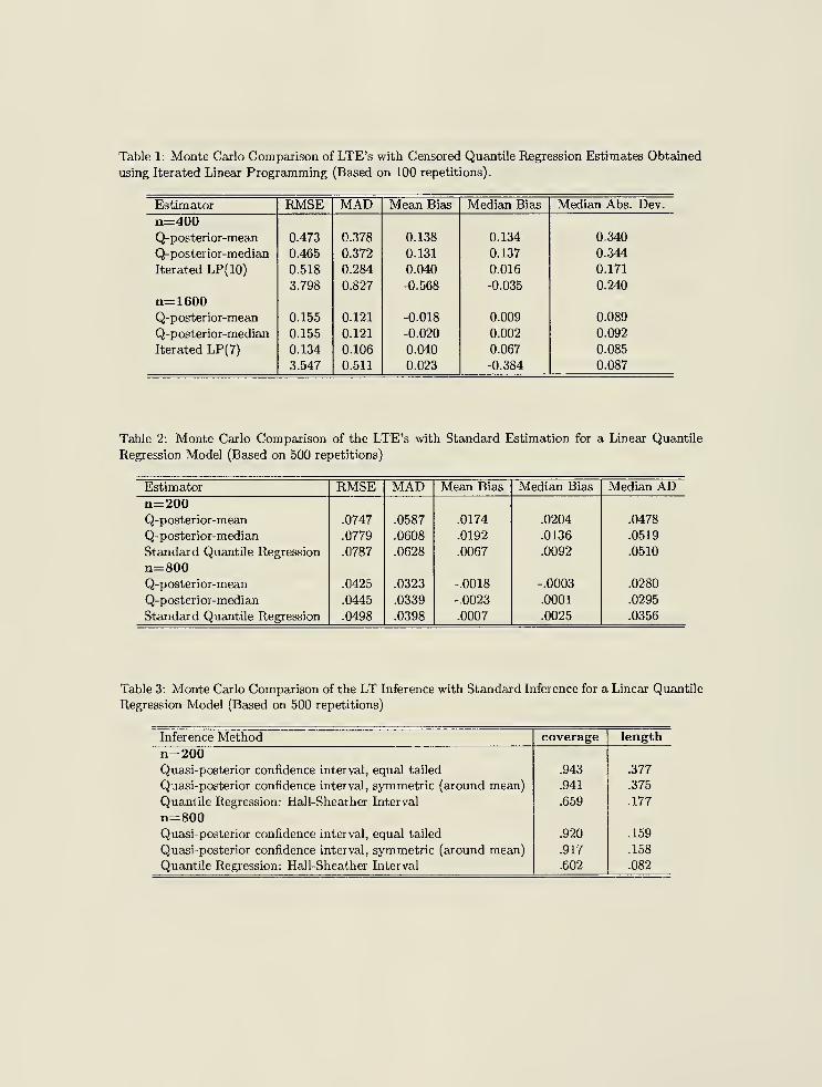
Table 1: Monte Carlo Comparison of LTE's with Censored Quantile Regression Estimates Obtained

using Iterated Linear Programming (Based on 100 repetitions).

Estimator RMSE MAD Mean Bias Median Bias Median Abs. Dev.

n=400Q-posterior-mean 0.473 0.378 0.138 0.134 0.340

Q-posterior-median 0.465 0.372 0.131 0.137 0.344

Iterated LP(10) 0.518 0.284 0.040 0.016 0.171

3.798 0.827 -0.568 -0.035 0.240

n=1600Q-posterior-mean 0.155 0.121 -0.018 0.009 0.089

Q-posterior-median 0.155 0.121 -0.020 0.002 0.092

Iterated LP(7) 0.134 0.106 0.040 0.067 0.085

3.547 0.511 0.023 -0.384 0.087

Table 2: Monte Carlo Comparison of the LTE's with Standard Estimation for a Linear Quantile

Regression Model (Based on 500 repetitions)

Estimator RMSE MAD Mean Bias Median Bias Median ADn=200Q-posterior-mean .0747 .0587 .0174 .0204 .0478

Q-posterior-median .0779 .0608 .0192 .0136 .0519

Standard Quantile Regression .0787 .0628 .0067 .0092 .0510

n=800Q-posterior-mean .0425 .0323 -.0018 -.0003 .0280

Q-posterior-median .0445 .0339 -.0023 .0001 .0295

Standard Quantile Regression .0498 .0398 .0007 .0025 .0356

Table 3: Monte Carlo Comparison of the LT Inference with Standard Inference for a Linear Quantile

Regression Model (Based on 500 repetitions)

Inference Method coverage length

n=200Quasi-posterior confidence interval, equal tailed .943 .377

Quasi-posterior confidence interval, symmetric (around mean) .941 .375

Quantile Regression: Hall-Sheather Interval .659 .177

n=800Quasi-posterior confidence interval, equal tailed .920 .159

Quasi-posterior confidence interval, symmetric (around mean) .917 .158

Quantile Regression: Hall-Sheather Interval .602 .082

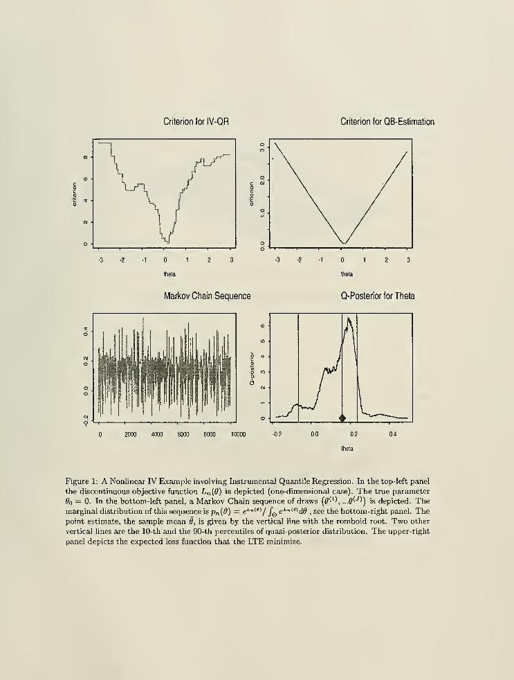
Criterion for IV-QR Criterion for QB-Estimation

CO •

\ psto

<*

CM

O

"\J

i4

thela

Markov Chain Sequence

12 3

theta

Q-Posterior for Theta

2000 4000 6000 8000 10000 -0.2 0.0 0.2

thela

0.4

Figure 1: A Nonlinear IV Example involving Instrumental Quantile Regression. In the top-left panel

the discontinuous objective function Ln {0) is depicted (one-dimensional case). The true parameter

#o = 0. In the bottom-left panel, a Markov Chain sequence of draws (0'1', ...0^) is depicted. The

marginal distribution of this sequence is pn {9) = eL " (8)

/ /e eLnWd0 , see the bottom-right panel. Thepoint estimate, the sample mean 9, is given by the vertical line with the romboid root. Two other

vertical lines are the 10-th and the 90-th percentiles of quasi-posterior distribution. The upper-right

panel depicts the expected loss function that the LTE minimize.

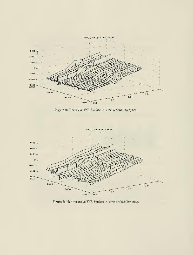
Var(p) for dynamic model

24-00 o.2

Figure 2: Recursive VaR Surface in time-probability space

Var(p) for static model

2400 0.2

Figure 3: Non-recursive VaR Surface in time-probability space

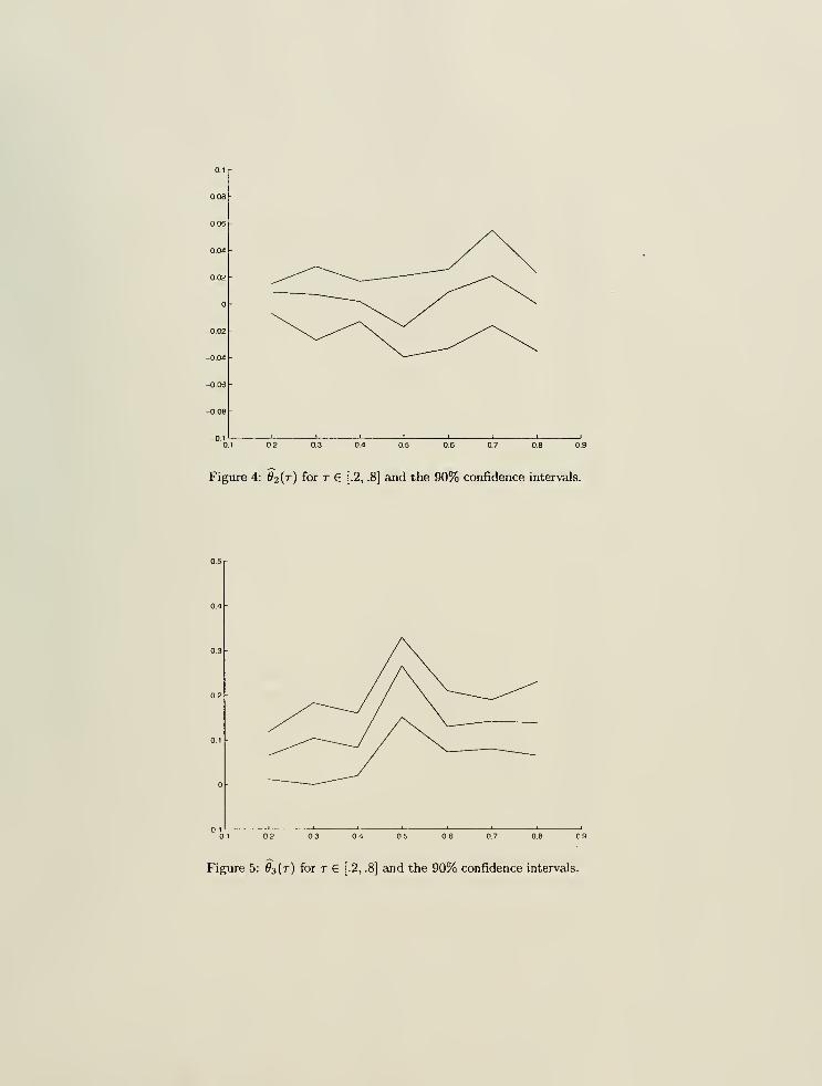
Figure 4: 9?(t) for r € [.2, .8] and the 90% confidence intervals.

Figure 5: #3(7") for r G [.2, .8] and the 90% confidence intervals.

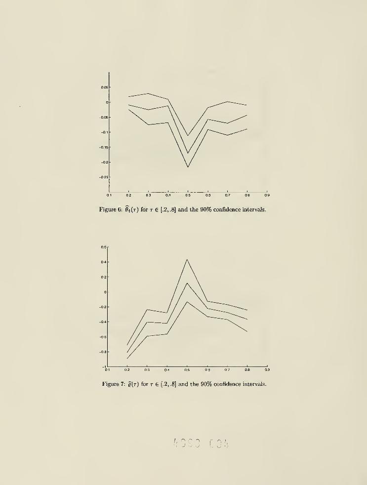
0.1 0.2 0.3 0.4 0.6 0.7

Figure 6: d\ (r) for r 6 [.2, .8] and the 90% confidence intervals.

0.1 0.2 0.3 0.4 0:5 0.6 0.8 0.9

Figure 7: q(t) for t e [.2, .8] and the 90% confidence intervals.

^8 38 G[

'

I 1 2003

Date Due

Lib-26-67

MIT LIBRARIES

3 9080 02613 1380