A MCMC APPROACH TO CLASSICAL ESTIMATION

VICTOR CHERNOZHUKOV∗ AND HAN HONG∗∗

Abstract. This paper studies the class of practical estimators that we refer to as the

Generalized Laplacian or Quasi-Bayesian estimators (hereafter GLE). The GLE’s include

means, medians, and quantiles of quasi-posterior distributions derived from econometric

criterion functions, such as those in GMM, median regression, nonlinear instrumental

variables, generalized empirical likelihood, minimum distance, and other problems. When

the underlying objective function is a log likelihood function of the data, the estimator is

equivalent to the canonical Bayesian approach. More generally, objective functions, such as

those of GMM and other semi-parametric estimators, can be used to form quasi-posterior

distributions about parameters.

The GLE’s are computationally attractive, and this alone represents a major practi-

cal motivation. They solve well-defined convex optimization problems even in nonlinear

models and are generically computable. The computation can be carried out by draw-

ing a sample from an appropriately transformed criterion function and simply taking the

means and medians, and possibly other moments of the resulting sample as point esti-

mates. Markov Chain Monte Carlo methods are easily adapted to these problems and

do not require any underlying likelihood formulation. Thus, GLE’s apply to a large class

of non-Bayesian problems, especially such important semi-parametric problems as cen-

sored median regression, instrumental median regression, the nonlinear IV estimation as

in models of Berry, Levinsohn, and Pakes (1995).

The GLE’s are shown to be√

n-consistent and asymptotically normal under weak condi-

tions, which allows discontinuous and non-differentiable criterion functions. Furthermore,

in a wide class of problems, the quasi-posterior quantiles are shown to provide asymptoti-

cally valid confidence intervals.

JEL Classifications: C10, C11, C13, C15

Key Words: GMM, extremum estimators, analogy principle, Bayes, Markov Chain Monte

Carlo, Censored LAD, Instrumental Median Regression

Date: November 1, 2002. We thank Jason Abrevaya, Gary Chamberlain, Jinyong Hahn, Chris Hansen,

Jerry Hausman, James Heckman, Shakeeb Kahn, Whitney Newey, Chris Sims, Ruey Tsay and seminar

participants in MIT-Harvard, University of Chicago, Princeton University, Wisconsin-Madison, University

of Michigan, Michigan State University, Texas-A&M, Brown University, the 2002 Atlanta winter meeting

of the Econometric Society, the 2002 European Econometric Society Meeting in Venice for insightful

comments.

1. Introduction

A variety of econometric problems pose not only a theoretical but, often importantly, apractical computational challenge. Some examples include Powell (1984)’s censored medianregression for linear and nonlinear problems, nonlinear GMM for the Berry, Levinsohn, andPakes (1995) model, the instrumental median regression, the continuous-updated GMM es-timator of Hansen, Heaton, and Yaron (1996), and related empirical likelihood estimators.These problems represent a formidable practical challenge as the extremum estimators areknown to be difficult to compute due to highly non-convex criterion functions with manylocal optima (but well pronounced global optimum). Despite extensive work to find resolu-tions to this problem, see for example Andrews (1997), the computational problem remainsdaunting in many applications.

This paper studies the statistical properties a class of estimators referred to as the Gen-eralized Laplacian estimators (GLE) or Quasi-Bayesian estimators (QBE). The GLE can beeasily computed using Markov Chain Monte Carlo (MCMC), a class of posterior simulationtechniques from bayesian statistics. This approach will be shown to yield both computableand theoretically attractive new estimators to such problems as (1) Powell’s censored me-dian regression, (2) instrumental median regression, (3) nonlinear IV in Berry, Levinsohn,and Pakes (1995), and others.

Our present motivation is rooted in the early work of Laplace (1774), who regarded atransformation of a least square criterion function as a statistical belief or distribution overa parameter of interest, and obtained point estimates as the means and medians of thatdistribution. He outlined the asymptotic normality and the large sample equivalence tothe extremum estimator of these alternative quantities. As noted by Stigler (1983), theargument did not rely on gaussianity of errors, and thus was not formally Bayesian. Whenthe likelihood is correct, the Laplacian approach is equivalent to the Bayesian approach.Laplace’s work became a basis for the so-called Laplace approximation, which explores inte-gral approximations for solving various extremum problems, or, vice versa, approximatingintegrals by certain extremum problems.1

The GLE are derived similarly and explore the same principle without relying on thelikelihood formulation. Given any statistical criterion function, we may transform it intoa proper distribution (quasi-posterior) over a parameter of interest and define various mo-ments of that distribution as the point estimates. In many cases, the quantiles of thisdistribution will be shown to yield asymptotically valid confidence intervals. For example,in the (instrumental) quantile regression setting, those intervals provide valid large sampleand good small sample inference without the estimation of the conditional density function.

1See Kusuoka and Liang (2000), Bolthausen (1986), citemcclure, Kolassa (1994) for example.

1

Note that the criterion function may be motivated by the analog principle, does not haveto be a likelihood (density) of the data, and most often is semi-parametric. The result-ing estimators possess a number of good theoretical properties and yield new, alternativeapproaches for the important problems mentioned earlier.

The computation of the estimator can be carried out by MCMC which simulates a seriesof parameter draws so that the marginal distribution of the series is approximately thequasi-posterior distribution of the parameters. Given this series, the estimator is given,depending on the choice of loss functions, either in the explicit form as the mean or thequantile of the series, or in the implicit form as minimizer of a smooth convex optimizationproblem.

An important property of the computation and estimation based on the MCMC meansand medians is that both the statistical and probabilistic structure of the problem is takeninto account, which helps to circumvent the computational curse of dimensionality. On theone hand, statistical considerations allow us to focus on computing means and quantiles inplace of modes (extremum estimates). On the other hand, probabilistic considerations inthe computation suggest that the mean or quantile of a nonparametric distribution can beestimated with the parametric rate 1/

√B, where B is the number of draws from a distri-

bution (functional evaluations). In sharp contrast, the mode (extremum) is estimated bythe MCMC and similar grid-based algorithms at the nonparametric rate B

− p2(d+p) , with d

denoting the parameter dimension and p the smoothness order. This rate worsens sharply(exponentially) in the dimension d of the optimization problem and as the underlying ob-jective function becomes less smooth, when p < 1, as in censored median regression orinstrumental median regression examples.

Another useful feature of Quasi-Bayesian estimation is that it provides a simple way totake into account the overall shape of the objective function and to construct confidenceregions simultaneously with the point estimates. It also allows incorporation of some priorinformation and imposition of constraints in the estimation procedure.

Given the attractive practical properties, an important question to investigate is theformal statistical properties of the estimators. This paper establishes

√n normality and

consistency of Laplace-type estimators, as well as the properties of the derived inferenceprocedures, under general conditions, extending the theoretical work on Bayesian estimatorsby Ibragimov and Has’minskii (1981). The obtained results are weak enough to cover theexamples listed above under general conditions that allow discontinuous, non-smooth semi-parametric criterion functions and general data generating processes.

The remainder of the paper proceeds as follows. Section 2 formally defines and furthermotivates the Laplace type estimators with several examples, reviews the literature, andexplains historical connections. The motivating examples, which are all semi-parametricand involve no parametric likelihoods, will justify the pursuit of a more general theory than

2

is currently available. Section 3 develops the large sample theory, and explores it within thecontext of the econometric examples mentioned earlier. Section 4 briefly reviews importantcomputational aspects and illustrates the use of the estimator through simulation examples.Section 5 contains a brief empirical example, and section 6 concludes.

2. Laplace or Quasi-Bayes Estimation: Definition and Motivation

2.1. Motivation. Extremum estimators are usually motivated by the analogy principleand are defined as maximizers over parameter space Θ of a random finite-sample criterionfunction Ln (θ), where n denotes the sample size. n−1Ln (θ) is viewed as a sample averagethat converges to a criterion function M (θ) that is maximized uniquely at some θ0 ∈ Θ.Extremum estimators are usually consistent and asymptotically normal, cf. Gallant andWhite (1988), Amemiya (1985) and Newey and McFadden (1994a). However, in manyimportant cases, actually implementing the extremum estimates remains a large problem.

Example 1 (Censored Quantile Regression). A prominent model in econometrics isthe censored median regression model of Powell (1984). As a special case of nonlinearquantile regression, the censored median regression estimator is defined to maximize Powell’scriterion function

Ln (β) = −n∑

i=1

ωi · ρτ (Yi −max (0, g(Xi;β)) ,

where ρτ (u) = (τ − 1(u < 0))u is the check function of Koenker and Bassett (1978), ωi

is a weight, and Yi is either positive or zero, so its conditional quantile is specified asmax(0, g(Xi, β)). The censored quantile regression model was first formulated by Powell(1984) as a way to provide valid inference in the Tobin-Amemiya models without distri-butional assumptions under heteroscedasticity of unknown form. The extremum estimatorbased on Powell’s criterion function, while theoretically elegant, has a well known compu-tational difficulty. The objective function is nonsmooth, highly nonconvex, with numerouslocal optima, posing a formidable obstacle to the practical use of the extremum estimator,see Buchinsky and Hahn (1998), Buchinsky (1991), Fitzenberger (1997), Khan and Pow-ell (2001) for related discussions. In this paper, we shall explore the use of alternative -quasi-bayesian - estimators based on the Powell objective function, and will show that thisalternative is attractive both theoretically and computationally.

Example 2 (Instrumental and Robust Median Regression). Early variant of instru-mental median regression can be found in Mood (1950). A modern version of this is definedby maximizing

Ln(θ) = −12

(1√n

n∑

i=1

mi(θ)

)′W (θ)

(1√n

n∑

i=1

mi(θ)

),

3

where

mi (θ) = (τ − 1(Yi ≤ q(Di, Xi, θ))Zi,

where Y is the dependent variable, D is a vector of possibly endogeneous variables, Zi isa vector of instruments, and W (θ) is a positive definite weighting matrix, e.g.

W (θ) =

[1n

n∑

i=1

mi (θ)mi (θ)′]−1

+ op (1) .

Motivations for estimating equations of this sort arise from the treatment effect modelsand simultaneous equation models, cf. Chernozhukov and Hansen (2001), as well as fromrobustness concerns.2 Clearly, a variety of Huber (1973)’s robust estimators can be definedsimilarly. For example, in the absence of endogeneity,

q(X, τ) = X ′β (τ) ,

Z = f(X) can be constructed to preclude the influence of outliers in X on the inference.

For example, choosing Zij = 1 (Xij < xj) , j = 1, . . . ,dim (X), where xj denotes themedian of Xij produces an approach that is similar in spirit to the maximal regressiondepth estimator of Rousseeuw and Wets (1999), whose computational difficulty is wellknown, as discussed in Van Aelst, Rousseeuw, Huber, and Struyf (2002). The resultingestimating objective function Ln (β) is highly robust to both outliers in Xij and Yi. In fact,it appears that breakdown properties of this objective function are very similar to those ofthe objective function of Rousseeuw and Wets (1999).

Despite a clear appeal, the daunting problem is computational. The function Ln is almosteverywhere flat and has numerous discontinuities and local optima. Figure 1 illustrates thesituation. (Note that the global optimum is well pronounced.) Figure 1 illustrates thesituation. Again, in this case the GLE approach will yield a computable and theoreticallyattractive alternative to extremum estimation. Furthermore, we will show that the quasi-posterior confidence intervals provide a valid and effective way to construct confidenceintervals for parameters and their smooth functions without estimating the conditionaldensity function evaluated at quantiles.

2Note that the classical Koenker-Bassett’s quantile regression does not apply in the endogenous case or

in cases when X has a Cauchy distribution (without truncation). See Chernozhukov and Hansen (2001)

for an extension of Koenker and Bassett’s approach to instrumental problems like these. Note that this

extension however exploits the fact that the dimension of the parameter in front of endogenous variables is

low, which is the case in many applications, but is not the case in problems like HS(2002) where dimension

of endogenous variable is high.

4

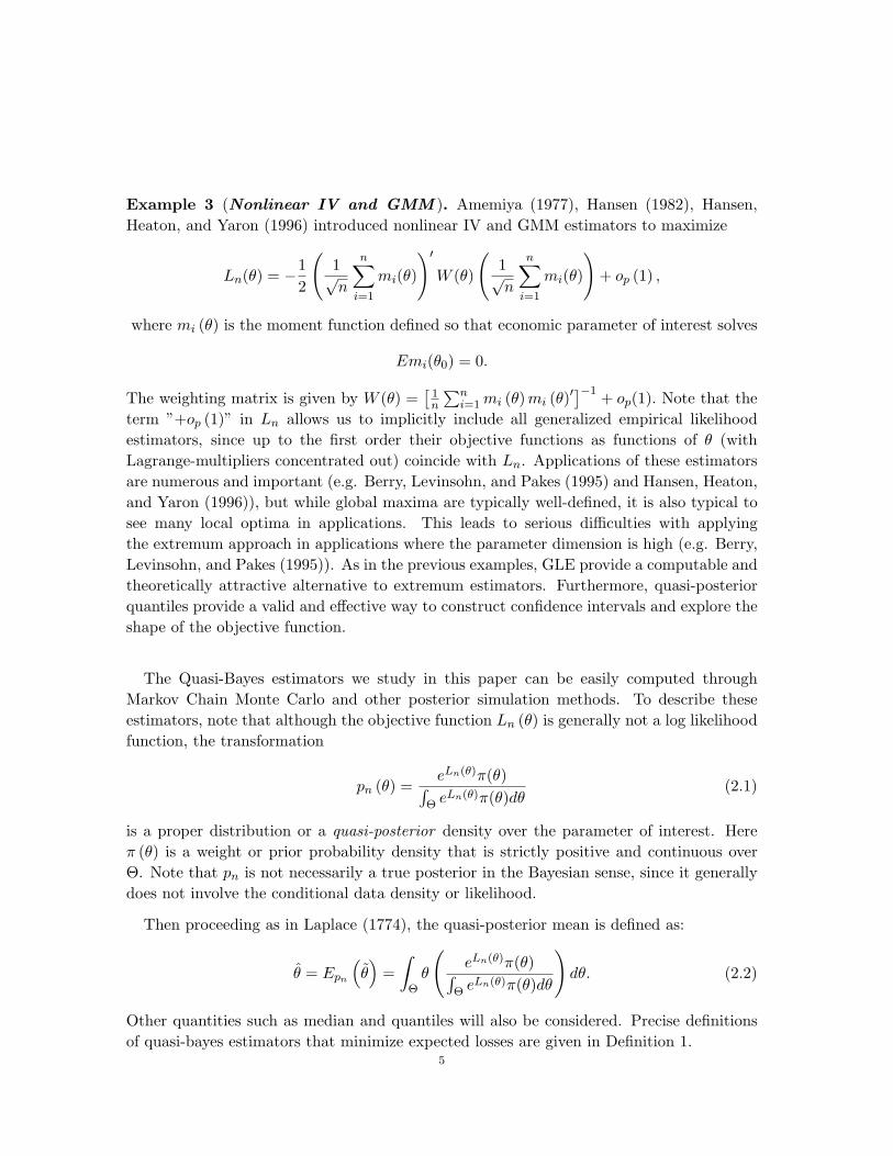
Example 3 (Nonlinear IV and GMM ). Amemiya (1977), Hansen (1982), Hansen,Heaton, and Yaron (1996) introduced nonlinear IV and GMM estimators to maximize

Ln(θ) = −12

(1√n

n∑

i=1

mi(θ)

)′W (θ)

(1√n

n∑

i=1

mi(θ)

)+ op (1) ,

where mi (θ) is the moment function defined so that economic parameter of interest solves

Emi(θ0) = 0.

The weighting matrix is given by W (θ) =[

1n

∑ni=1 mi (θ)mi (θ)

′]−1 + op(1). Note that theterm ”+op (1)” in Ln allows us to implicitly include all generalized empirical likelihoodestimators, since up to the first order their objective functions as functions of θ (withLagrange-multipliers concentrated out) coincide with Ln. Applications of these estimatorsare numerous and important (e.g. Berry, Levinsohn, and Pakes (1995) and Hansen, Heaton,and Yaron (1996)), but while global maxima are typically well-defined, it is also typical tosee many local optima in applications. This leads to serious difficulties with applyingthe extremum approach in applications where the parameter dimension is high (e.g. Berry,Levinsohn, and Pakes (1995)). As in the previous examples, GLE provide a computable andtheoretically attractive alternative to extremum estimators. Furthermore, quasi-posteriorquantiles provide a valid and effective way to construct confidence intervals and explore theshape of the objective function.

The Quasi-Bayes estimators we study in this paper can be easily computed throughMarkov Chain Monte Carlo and other posterior simulation methods. To describe theseestimators, note that although the objective function Ln (θ) is generally not a log likelihoodfunction, the transformation

pn (θ) =eLn(θ)π(θ)∫

Θ eLn(θ)π(θ)dθ(2.1)

is a proper distribution or a quasi-posterior density over the parameter of interest. Hereπ (θ) is a weight or prior probability density that is strictly positive and continuous overΘ. Note that pn is not necessarily a true posterior in the Bayesian sense, since it generallydoes not involve the conditional data density or likelihood.

Then proceeding as in Laplace (1774), the quasi-posterior mean is defined as:

θ = Epn

(θ)

=∫

Θθ

(eLn(θ)π(θ)∫

Θ eLn(θ)π(θ)dθ

)dθ. (2.2)

Other quantities such as median and quantiles will also be considered. Precise definitionsof quasi-bayes estimators that minimize expected losses are given in Definition 1.

5

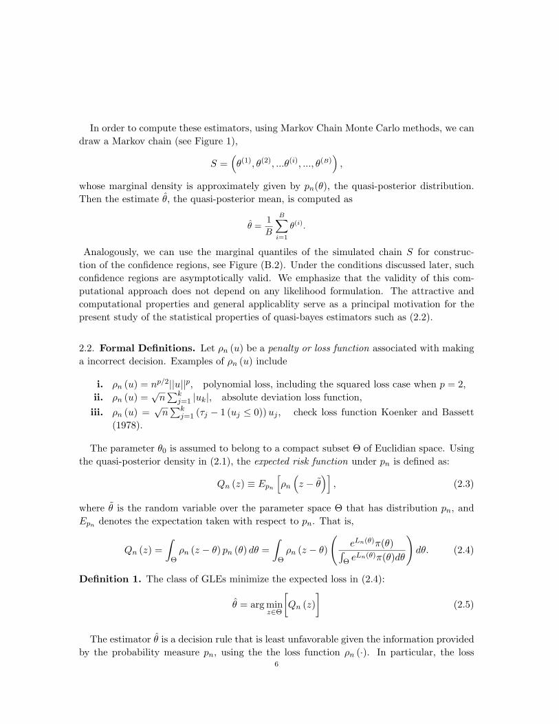
In order to compute these estimators, using Markov Chain Monte Carlo methods, we candraw a Markov chain (see Figure 1),

S =(θ(1), θ(2), ...θ(i), ..., θ(B)

),

whose marginal density is approximately given by pn(θ), the quasi-posterior distribution.Then the estimate θ, the quasi-posterior mean, is computed as

θ =1B

B∑

i=1

θ(i).

Analogously, we can use the marginal quantiles of the simulated chain S for construc-tion of the confidence regions, see Figure (B.2). Under the conditions discussed later, suchconfidence regions are asymptotically valid. We emphasize that the validity of this com-putational approach does not depend on any likelihood formulation. The attractive andcomputational properties and general applicablity serve as a principal motivation for thepresent study of the statistical properties of quasi-bayes estimators such as (2.2).

2.2. Formal Definitions. Let ρn (u) be a penalty or loss function associated with makinga incorrect decision. Examples of ρn (u) include

i. ρn (u) = np/2||u||p, polynomial loss, including the squared loss case when p = 2,ii. ρn (u) =

√n

∑kj=1 |uk|, absolute deviation loss function,

iii. ρn (u) =√

n∑k

j=1 (τj − 1 (uj ≤ 0)) uj , check loss function Koenker and Bassett(1978).

The parameter θ0 is assumed to belong to a compact subset Θ of Euclidian space. Usingthe quasi-posterior density in (2.1), the expected risk function under pn is defined as:

Qn (z) ≡ Epn

[ρn

(z − θ

)], (2.3)

where θ is the random variable over the parameter space Θ that has distribution pn, andEpn denotes the expectation taken with respect to pn. That is,

Qn (z) =∫

Θρn (z − θ) pn (θ) dθ =

∫

Θρn (z − θ)

(eLn(θ)π(θ)∫

Θ eLn(θ)π(θ)dθ

)dθ. (2.4)

Definition 1. The class of GLEs minimize the expected loss in (2.4):

θ = arg minz∈Θ

[Qn (z)

](2.5)

The estimator θ is a decision rule that is least unfavorable given the information providedby the probability measure pn, using the the loss function ρn (·). In particular, the loss

6

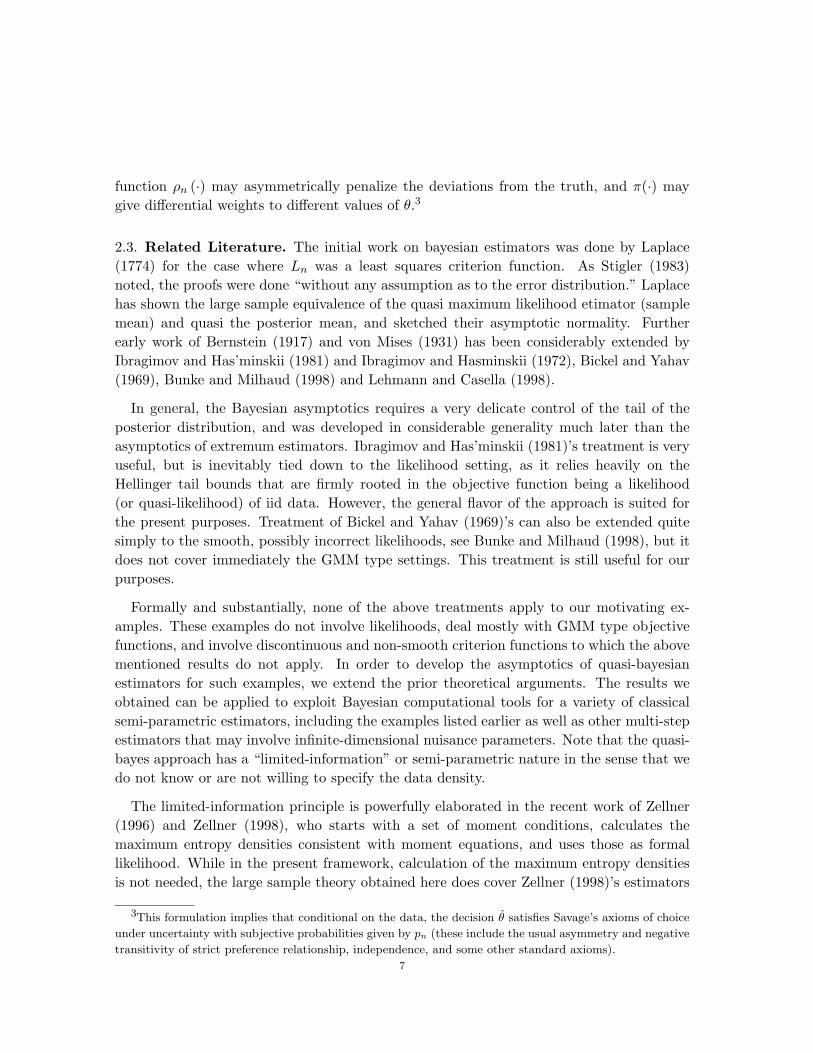
function ρn (·) may asymmetrically penalize the deviations from the truth, and π(·) maygive differential weights to different values of θ.3

2.3. Related Literature. The initial work on bayesian estimators was done by Laplace(1774) for the case where Ln was a least squares criterion function. As Stigler (1983)noted, the proofs were done “without any assumption as to the error distribution.” Laplacehas shown the large sample equivalence of the quasi maximum likelihood etimator (samplemean) and quasi the posterior mean, and sketched their asymptotic normality. Furtherearly work of Bernstein (1917) and von Mises (1931) has been considerably extended byIbragimov and Has’minskii (1981) and Ibragimov and Hasminskii (1972), Bickel and Yahav(1969), Bunke and Milhaud (1998) and Lehmann and Casella (1998).

In general, the Bayesian asymptotics requires a very delicate control of the tail of theposterior distribution, and was developed in considerable generality much later than theasymptotics of extremum estimators. Ibragimov and Has’minskii (1981)’s treatment is veryuseful, but is inevitably tied down to the likelihood setting, as it relies heavily on theHellinger tail bounds that are firmly rooted in the objective function being a likelihood(or quasi-likelihood) of iid data. However, the general flavor of the approach is suited forthe present purposes. Treatment of Bickel and Yahav (1969)’s can also be extended quitesimply to the smooth, possibly incorrect likelihoods, see Bunke and Milhaud (1998), but itdoes not cover immediately the GMM type settings. This treatment is still useful for ourpurposes.

Formally and substantially, none of the above treatments apply to our motivating ex-amples. These examples do not involve likelihoods, deal mostly with GMM type objectivefunctions, and involve discontinuous and non-smooth criterion functions to which the abovementioned results do not apply. In order to develop the asymptotics of quasi-bayesianestimators for such examples, we extend the prior theoretical arguments. The results weobtained can be applied to exploit Bayesian computational tools for a variety of classicalsemi-parametric estimators, including the examples listed earlier as well as other multi-stepestimators that may involve infinite-dimensional nuisance parameters. Note that the quasi-bayes approach has a “limited-information” or semi-parametric nature in the sense that wedo not know or are not willing to specify the data density.

The limited-information principle is powerfully elaborated in the recent work of Zellner(1996) and Zellner (1998), who starts with a set of moment conditions, calculates themaximum entropy densities consistent with moment equations, and uses those as formallikelihood. While in the present framework, calculation of the maximum entropy densitiesis not needed, the large sample theory obtained here does cover Zellner (1998)’s estimators

3This formulation implies that conditional on the data, the decision θ satisfies Savage’s axioms of choice

under uncertainty with subjective probabilities given by pn (these include the usual asymmetry and negative

transitivity of strict preference relationship, independence, and some other standard axioms).

7

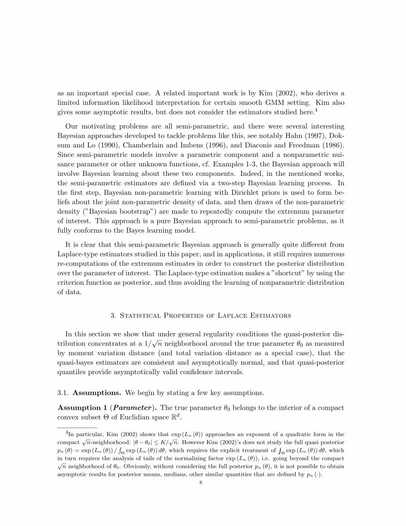
as an important special case. A related important work is by Kim (2002), who derives alimited information likelihood interpretation for certain smooth GMM setting. Kim alsogives some asymptotic results, but does not consider the estimators studied here.4

Our motivating problems are all semi-parametric, and there were several interestingBayesian approaches developed to tackle problems like this, see notably Hahn (1997), Dok-sum and Lo (1990), Chamberlain and Imbens (1996), and Diaconis and Freedman (1986).Since semi-parametric models involve a parametric component and a nonparametric nui-sance parameter or other unknown functions, cf. Examples 1-3, the Bayesian approach willinvolve Bayesian learning about these two components. Indeed, in the mentioned works,the semi-parametric estimators are defined via a two-step Bayesian learning process. Inthe first step, Bayesian non-parametric learning with Dirichlet priors is used to form be-liefs about the joint non-parametric density of data, and then draws of the non-parametricdensity (”Bayesian bootstrap”) are made to repeatedly compute the extremum parameterof interest. This approach is a pure Bayesian approach to semi-parametric problems, as itfully conforms to the Bayes learning model.

It is clear that this semi-parametric Bayesian approach is generally quite different fromLaplace-type estimators studied in this paper, and in applications, it still requires numerousre-computations of the extremum estimates in order to construct the posterior distributionover the parameter of interest. The Laplace-type estimation makes a ”shortcut” by using thecriterion function as posterior, and thus avoiding the learning of nonparametric distributionof data.

3. Statistical Properties of Laplace Estimators

In this section we show that under general regularity conditions the quasi-posterior dis-tribution concentrates at a 1/

√n neighborhood around the true parameter θ0 as measured

by moment variation distance (and total variation distance as a special case), that thequasi-bayes estimators are consistent and asymptotically normal, and that quasi-posteriorquantiles provide asymptotically valid confidence intervals.

3.1. Assumptions. We begin by stating a few key assumptions.

Assumption 1 (Parameter). The true parameter θ0 belongs to the interior of a compactconvex subset Θ of Euclidian space Rd.

4In particular, Kim (2002) shows that exp (Ln (θ)) approaches an exponent of a quadratic form in the

compact√

n-neighborhood: |θ− θ0| ≤ K/√

n. However Kim (2002)’s does not study the full quasi posterior

pn (θ) = exp (Ln (θ)) /RΘ

exp (Ln (θ)) dθ, which requires the explicit treatment ofRΘ

exp (Ln (θ)) dθ, which

in turn requires the analysis of tails of the normalizing factor exp (Ln (θ)), i.e. going beyond the compact√n neighborhood of θ0. Obviously, without considering the full posterior pn (θ), it is not possible to obtain

asymptotic results for posterior means, medians, other similar quantities that are defined by pn (·).8

Assumption 2 (Penalty Function). The penalty function ρn satisfies the following con-ditions:

i. ρn(u) is of the form ρ(anu), where ρ(u) ≥ 0 and = 0 iff u = 0, and an =√

n

ii. ρ is convex and ρ(h) ≤ 1 + ‖h‖p for some p > 0.

iii. ϕ (ξ) =∫Rd ρ(u− ξ)e−u′audu is minimized uniquely at some ξ∗ ∈ Rd for any a > 0.

Assumption 3 (Identification). For any δ > 0, there exists ε > 0, such that

limn→∞P

sup

|θ−θ0|≥δ

1n

(Ln (θ)− Ln (θ0)

)≤ −ε

= 1.

Assumption 4 (Local Asymptotic Normality). For θ in an open neighborhood of θ0,

i. Ln (θ)− Ln (θ0) = (θ − θ0)′∆n (θ0)− 1

2 (θ − θ0)′ [nJ (θ0)] (θ − θ0) + Rn (θ),

ii. ∆n (θ0) /√

nd−→ N (0, Ω),

iii. Ω and J (θ0) are positive definite constant matrices,

iv. for each ε > 0 there is sufficiently small δ > 0 and large M > 0 such that

(a) lim supn

P

sup

M/√

n≤|θ−θ0|≤δ

|Rn (θ) |n|θ − θ0|2 > ε

< ε,

(b) lim supn

P

sup

|θ−θ0|≤M/√

n

|Rn (θ) | > ε

= 0.

In general, our assumptions are related but are different from those in Bickel and Yahav(1969) and Ibragimov and Has’minskii (1981). The most substantial differences appear inassumption 4, where we introduce Huber-like control conditions to handle the tail behaviorof discontinuous and non-smooth criterion functions. In general, the early approaches, suchas that of Ibragimov and Has’minskii (1981), are inevitably tied down to the likelihoodformulation as they rely upon various inequalities put forward onto the Hellinger-distancebetween the true density and the density at alternative parameter values, which is notentirely suited for the present purposes.

The compactness assumption 1 is conventional. That the parameter is on the interior ofthe parameter space helps to rule out non-regular cases, see for example Andrews (1999).

Assumption 2 impose convexity on the loss function. We do not consider the non-convexloss functions due to pragmatic reasons. One of the main motivation of this paper is the

9

generic computability of the estimates, given that they solve well-defined convex optimiza-tion problems. The domination condition, ρ (h) ≤ 1 + |h|p for some p > 0, is conventionaland is satisfied in all examples of ρ we gave. Note that this condition implicitly assumesthat the penalty function has been scaled by some constant so that this inequality holds.

The assumption that ϕ (ξ) =∫

ρ (u− ξ) e−u′audu = Eρ (N (0, a)− ξ) attains a uniqueminimum at some finite ξ∗ for any positive definite a, is the generalized Anderson condition,and it certainly holds for all examples of ρ we have. In fact, when ρ (·) is symmetric, ξ∗ = 0by Anderson’s lemma.

Assumption 3 is implied by usual uniform convergence and unique identification condi-tions as in Amemiya (1985). The proof of lemma 1 is can be found in Amemiya (1985).

Lemma 1. Assumption 3 holds when

i. M(θ) is continuous on Θ and has unique maximum at θ0

ii. Ln (θ) /n converges uniformly in Θ to M (θ).

Assumption 4 does not require differentiablity of the criterion function and holds underfairly general conditions. Assumption 4.ii requires asymptotic normality to hold, and is gen-erally a weak assumption for cross-sectional and many time-series applications. Assumption4.iii rules out the cases of the mixed asymptotic normality for some non-stationary timeseries models. It can potentially be extended to allow for nonlinear dynamic models asthose in Gallant and White (1988).

Assumption 4.iv is a Huber-like stochastic equicontinuity condition, which requires thatthe remainder term of the expansion can be made small in a particular way over a neigh-borhood of θ0. There are many simple-to-verify sufficient conditions given in empiricalprocess literature, e.g. Van der Vaart and Wellner (1996) and Amemiya (1985), Andrews(1994), Newey (1991), and Pakes and Pollard (1989). In the subsequent sections we verifythis condition for all the examples discussed in the previous section. Clearly, Assumption4 holds under the usual differentiability condition as in Amemiya (1985), as illustrated inthe following lemma. The proof is lemma 2 is standard and hence omitted.

Lemma 2. Assumption (4) holds with

∆n(θ0) = ∇θLn(θ0) and J(θ0) = ∇θθ′M (θ0) , if

i. for some δ > 0, Ln (θ) and M (θ) are twice differentiable in θ when |θ − θ0| < δ,

ii. ∇θLn(θ0)/√

nd−→ N(0, Ω),

iii. for each ε > 0, there is δ > 0 such that

limn→∞

P

(sup

|θ−θ0|<δ

∣∣∣∣∇θθ′Ln (θ) /n−∇θθ′M (θ)∣∣∣∣ > ε

)= 0.

10

3.2. Convergence in the Total Variation of Moments Norm. Under the assumptions1-4, we show that the quasi-posterior density concentrates at a 1/

√n neighborhood of θ0

in a ”total variation of moments” norm, and then use this result to obtain asymptoticnormality of the quasi-Bayes estimate.

To describe this result we introduce some notations. Define the local parameter h as anormalized deviation from θ0 and centered at the normalized random “score function”:

h =√

n (θ − θ0)− J (θ0)−1 ∆n (θ0) /

√n.

Define by the Jacobi rule localized quasi-posterior density for h as

p∗n (h) =1√n

pn

(h/√

n + θ0 + J (θ0)−1 ∆n (θ0) /n

)

Define the total variation of moments norm or a measurable function f : S → R withsupport S ∈ Rd as

||f ||TMV (α) =∫

S(1 + |h|α) |f (h) |dh.

Theorem 1. (Convergence of Moments) Under assumptions 1 - 4, for any 0 ≤ α < ∞,

||p∗n (h)− p∗∞ (h) ||TMV (α) =∫

Hn

(1 + |h|α

)∣∣∣p∗n(h)− p∗∞(h)∣∣∣dh →p 0,

where Hn = √n(θ − θ0 − J (θ0)−1 ∆n (θ0) /n) : θ ∈ Θ and

p∗∞(h) =√|J(θ0)|√(2π)d

· exp(−1

2h′J(θ0)h

).

Theorem 1 shows that pn (θ) is concentrated at a 1/√

n neighborhood of θ0 as measured bythe total variation of moments norm. For large n, pn (θ) is approximately a random normaldensity with the random mean parameter θ0 + J (θ0)

−1 ∆n (θ0) /n, and constant varianceparameter J(θ0)−1/n. Theorem 1 includes the classical likelihood settings as an importantcase, in particular implying the Berstein-Von Mises Theorems for the posterior likelihood,which state the convergence of the posterior to the limit random density in the total variationnorm:

||p∗n (h)− p∗∞ (h) ||TMV (0) =‖p∗n − p∗∞‖TV

=∫

Hn

∣∣∣p∗n(h)− p∗∞(h)∣∣∣dh →p 0.

Convergence in the total variation norm is not sufficient for convergence of quasi-bayes esti-mators such as the posterior means. The stronger result in Theorem 1 allows for convergenceof any α-th posterior moment.

11

3.3. Limit Theory for Point Estimates and Confidence Intervals. As a direct conse-quence of Theorem 1, the next theorem establishes

√n- consistency and asymptotic normal-

ity of the qausi-bayes estimator. When the loss function ρ (·) is symmetric, the quasi-Bayesestimator is asymptotically equivalent to the extremum estimator and is asymptoticallynormal with mean zero. Recall that asymmetric penalty functions are interesting for thepurposes of describing the behavior of posterior quantiles.

In order to describe the result, let us define some important notations. Recall that theextremum estimator

√n

(θex − θ0

)is first order-equivalent to:

Wn ≡ 1√n

J (θ0)−1 ∆n (θ0) .

given that the p∗n approaches p∗∞, it may be expected that the quasi-Bayes estimator√n

(θ − θ0

)is asymptotically equivalent to

Zn = arg minz

[∫

Rd

ρ (z − u) p∗∞(u−Wn) du

].

Define the constant ξJ(θ0) ∈ Rd as

ξJ(θ0) = arg minz∈Rd

[∫

Rd

ρ (z − u) p∗∞ (u) du

],

which exists by Assumption 2. For example, in the univariate case, if ρ (h) = (α− 1 (h < 0))h,the constant ξJ(θ0) = qαJ (θ0)

−1/2, where qα is the α-quantile of N (0, 1). If ρ is symmetric,i.e. ρ (h) = ρ (−h), then by Anderson’s lemma

ξJ(θ0) = 0.

It follows that

Zn = ξJ(θ0) + Wn,

and we are prepared to state the result.

Theorem 2. (GLE in Large Sample) Under assumptions 1-4,√

n(θ − θ0

)= ξJ(θ0) + Wn + op (1) ,

and

Wn →d W = N(0, J (θ0)

−1 Ω(θ0) J (θ0)−1

).

Furthermore, if ρ is symmetric, i.e. ρ (h) = ρ(−h) for all h, ξJ(θ0) = 0.

In order for the quasi-posterior distribution to provide valid large sample confidenceinterval from the classical point of view, the density of W should coincide with that of

12

p∗∞ (h). This requires∫

Rd

hh′p∗∞(h)dh ≡ J(θ0)−1 = Var(W ) ≡ J(θ0)−1Ω(θ0)J(θ0)−1,

or equivalently

Ω(θ0) = J(θ0),

which is a generalized information matrix equality. It is known to hold for regular, cor-rectly specified likelihoods. It is also known to hold for appropriately constructed criterionfunctions of generalized method of moments, minimum distance estimators, generalizedempirical likelihood estimators, and properly weighted extremum estimators.

Consider construction of the confidence intervals for the quantity g(θ0), and g is contin-uously differentiable at θ0. Define

Fg,n(x) =∫

θ∈Θ:g(θ)≤xpn(θ)dθ. and Qg,n(α) = infx : Fg,n(x) ≥ α.

Then a quasi-bayesian confidence interval is given by

[Qg,n(α/2), Qg,n(1− α/2)] .

Consider now the usual asymptotic intervals based on the Delta-method and any estimatorwith the property

√n(θ − θ) = J(θ0)−1∆n(θ)/

√n + op(1).

Such intervals are usually given by[g(θ) + qα/2

√∇θg(θ)T J(θ)−1∇θg(θ)√

n, g(θ) + q1−α/2

√∇θg(θ))T J(θ)−1∇θg(θ)√

n

],

where qα is the α-quantile of the standard normal distribution . The following Theoremestablishes the large sample validity of quasi-posterior confidence intervals.

Theorem 3. (Confidence Intervals) Suppose Assumptions 1-4 hold. In addition supposethat the generalized information matrix equality holds:

J(θ0) = Ω(θ0).

The quasi-posterior confidence intervals are first-order equivalent to the asymptotic inter-vals: for any α and J(θ) →p J(θ0)

Qg,n(α)− g(θ)− qα

√∇θg(θ)T J(θ)∇θg(θ)√

n= op(

1√n

),

so that

limn→∞P

Qg,n (α/2) ≤ g (θ0) ≤ Qg,n (1− α/2)

= 1− α.

13

As discussed in the next section, this confidence interval can be constructed using thequantiles of sequence of MCMC draws. Note that the generalized information matrix equal-ity is relatively easy to achieve within the method-of-moments, minimum-distance, andgeneralized empirical likelihood frameworks. The next section reviews the applications.

3.4. Generalized Method of Moments and Nonlinear Instrumental Variables.Going back to Example 3, recall that a typical economic model that underlies the applica-tions of GMM is a set population moment equations:

Emi(θ) = 0. if and only if θ = θ0 (3.1)

Method of moment estimators involve maximizing an objective function of the form

Ln (θ) = −12n (gn (θ))′Wn(θ) (gn (θ)) + op (1) , gn (θ) =

1n

n∑

i=1

mi (θ) , (3.2)

Wn(θ) = W (θ) + op(1), uniformly in θ ∈ Θ, (3.3)

W (θ) =[limn

Var[√

ngn(θ)]]−1

> 0 and continuous uniformly in θ ∈ Θ. (3.4)

Note that this choice of the weight matrix guarantees the generalized information matrixequality under standard regularity conditions.

Generally, by a Central Limit Theorem√

ngn(θ0) →d N(0,W−1(θ0)), (3.5)

so that the objective function transformed into a posterior pn(θ) = eLn(θ)∫Θ eLn(θ)dθ,

which can be interpreted as the approximate likelihood for the sample moments of the datagn(θ). Thus we can think of GMM as an approach that specifies the approximate likelihoodfor selected moments of the data without specifying the likelihood of the entire data.

We may impose Assumption 1-4 directly on the GMM objective function. However, tohighlight the plausibility and elaborate on the examples that satisfy Assumption 4 considerthe following set of simple conditions. The following proposition verifies the assumptions ofTheorems 1 - 3.

Proposition 1. (Method-of-Moments and Nonlinear IV) Suppose that Assumptions1-2 hold, and that in an open neighborhood of θ0, mi (θ) is stationary and ergodic, and

i. conditions (3.1)-(3.4) holds,

ii. J(θ) = G(θ)′W (θ)G(θ) > 0 and continuous, G(θ) = ∇θEmi(θ) is continuous,

iii. ∆n(θ0) = −√ngn(θ0)W (θ0)G(θ0) →d N(0, Ω(θ0)), and Ω(θ0) = G(θ0)′W (θ0)G(θ0),

14

iv. For any ε > 0, there is δ > 0, such that

lim supn→∞

P

sup

|θ−θ0|≤δ

√n| (gn(θ)− gn(θ0))− (Egn(θ)−Egn(θ0)) |

1 +√

n|θ − θ0| > ε

< ε (3.6)

Then Assumptions 3 and 4 hold. In addition the information matrix equality holds, sinceby construction of Wn,

J (θ0) = Ω (θ0) .

Therefore all of the conclusions of Theorems 1-3 hold, with ∆n, Ω(θ0) and J(θ0) definedabove.

For twice continuously differentiable smooth moment conditions, the smoothness condi-tions on ∇θLn(θ) and ∇θθ′Ln(θ) stated in lemma 2 guarantees condition (iv) in proposition1. More generally, Andrews (1994), Pakes and Pollard (1989) and Van der Vaart and Well-ner (1996) provided us with many methods to verify condition (iv) in a widest variety ofmethod-of-moments models.

Therefore, for symmetric loss functions, the quasi-Bayesian estimator is asymptoticallyequivalent to the GMM estimator. Furthermore, by construction generalized informationequality holds, and quasi-posterior quantiles provide a computationally attractive methodof “inverting” the objective function for the asymptotic confidence intervals.

Example 2 Continued Instrumental median regression falls outside either classicalBayesian approach and the classical approach of Amemiya. Yet the conditions of proposition1 are satisfied under mild conditions:

i. (Yi, Di, Xi, Zi) is iid data sequence, E[mi(θ0)Zi] = 0, and θ0 is identifiable,

ii. mi(θ) = (τ − 1(Y ≤ q(D, X, θ)))Z, θ ∈ Θ is Donsker, E supθ |mi(θ)|2 < ∞,

iii. G(θ) = ∇θEmi(θ) = EfY |D,X,Z(q(D,X, θ))Z∇θq(D, X, θ)′ is continuous,

iv. J(θ) = G(θ)′[Var mi(θ)]−1 G(θ) is continuous and p.d. in an open ball at θ0.

In this case we note that the weighting matrix can be taken to be

Wn =1

τ (1− τ)

[1n

n∑

i=1

ZiZ′i

]−1

,

in which case the information matrix equality will hold. Indeed, in this cas

Ω (θ0) = G (θ0)′W (θ0) G (θ0) = J (θ0) ,

where

W (θ0) = plimWn (θ0) = [Varmi (θ0)]−1 , Varmi (θ0) = τ (1− τ) EZiZ

′i.

15

When the model q is linear and the dimension of D is small, there is a variety of computableand practical estimators in the literature.5 In more general models, the arg-max estimatesare quite difficult to compute, and the inference faces a well-known difficulty of estimatingsparsity parameters, see Abadie (1995) for an in-depth discussion.

On the other hand, the quasi-posterior median and quantiles are easy to compute andprovide asymptotically valid confidence intervals. Note that the inference does not requirethe estimation of the density function. The simulation example given in section 4 stronglysupports the efficacy of the alternative approach.

A very important example with computational challenge is Berry, Levinsohn, and Pakes(1995). This example is very similar in nature to the instrumental quantile regression, andthe application of quasi-Bayesian methods may be fruitful there.

Example 3 Continued. From GMM to Generalized Empirical Likelihood. Aclass of objective functions that are first-order equivalent to those of GMM (after recenter-ing) can be formulated using the empirical likelihood framework.

A class of generalized empirical likelihood functions(GEL) are studied in Imbens, Spady,and Johnson (1998), Kitamura and Stutzer (1997), and Newey and Smith (2000). For a setof moment equations Emi(θ0) = 0 that satisfy the conditions of section 3.4, define

Ln(θ, γ) ≡n∑

i=1

(s(mi(θ)′γ

)− s (0)). (3.7)

Then set

Ln (θ) = Ln (θ, γ (θ)) ,

where γ(θ) solves

γ(θ) ≡ arg infγ∈Rp

Ln(θ, γ), (3.8)

where p = dim (mi).

The scalar function s(·) is strictly convex, finite, and three times differentiable functionon an open interval of R containing 0, denoted V, and is equal to +∞ outside such aninterval. s (·) is normalized so that both s′ (0) = 1 and s′′ (0) = 1. The choices of thefunction s(v) = − ln(1− v), exp(v), (1 + v)2/2 lead to the well-known empirical likelihood,exponential tilting, and continuously-updated GMM estimator.

Simple and practical sufficient conditions for the Amemiya type smoothness conditionstated in lemma 2 are given in Imbens, Spady, and Johnson (1998), Kitamura and Stutzer

5These include the “inverse” quantile regression approach in Chernozhukov and Hansen (2001), which is

an extension of Koenker and Bassett (1978)’s quantile regression to endogenuous settings.

16

(1997), including stationary weakly dependent data, Newey and Smith (2000) and Christof-fersen, Hahn, and Inoue (1999). Thus the applications of quasi-Bayesian estimators to theseproblems is immediate.

To illustrate the use of the Laplacian approach we state a set of simple conditions gearedtowards the non-smooth micro-econometric applications such as the instrumental medianregression problem. These regularity conditions imply the first order equivalence of theGEL and GMM objective functions.

Proposition 2. Suppose that Assumptions 1 and 2 hold, and that the following conditionsare satisfied: for some δ > 0 and all θ ∈ Θ

i. condition (3.1) holds and that mi (θ) is iid,

ii. P [mi (θ) < x] is continuously differentiable in θ for all |x| < K,

iii. sup|θ−θ0|<δ |mi (θ) | < K a.s.

iv. mi (θ) , θ ∈ Θ is a Donsker class, so that gn (θ0) = 1√n

∑ni=1 mi (θ0) →d N (0, V (θ0)),

then assumption 4 holds, and thus the conclusions of Theorems 1-3 are true with

∆n (θ0) /√

n = gn (θ0) V (θ0)−1G(θ0) →d N(0, Ω(θ0)),

Ω(θ0) = G(θ0)′V (θ0)−1G(θ0),

J(θ0) = G(θ0)′V (θ0)−1G(θ0), G(θ0) = E∇θmi(θ0).

Note that the information matrix equality holds in this case.

3.5. M-estimators. M-estimators, which include many linear and nonlinear regressions asspecial cases, typically maximize objective functions of the form

Ln (θ) =n∑

i=1

mi (θ) .

mi (θ) need not be the log likelihood function of observation i, and may depend on prelim-inary non-parametric estimation. Assumptions 1–3 usually are satisfied by uniform lawsof large numbers and by unique identification of the parameter, see for example Amemiya(1985) and Newey and McFadden (1994a). The next proposition gives a simple set ofsufficient conditions for assumption 4.

Proposition 3. Let mi (θ) be Suppose Assumptions 1-3 hold for the criterion functionspecified above with the following additional conditions: for θ in an open neighborhood ofθ0, mi (θ) is stationary and ergodic, and

17

i. there exists vector mi(θ0) such that Emi(θ0) = 0 and, for some δ > 0,

mi(θ)−mi(θ0)− mi(θ0)′(θ − θ0)|θ − θ0| : |θ − θ0| < δ

is Donsker,

E[mi(θ)−mi(θ0)− mi(θ0)′(θ − θ0)]2 = o(|θ − θ0|2),

ii. J(θ) = ∇θθ′E[mi(θ)] is continuous and nonsingular around θ0,

iii. ∆n (θ0) /√

n =∑n

i=1 mi(θ0)/√

n →d N(0,Ω(θ0)).

Then Assumption 4 holds. Therefore, conclusions of Theorems 1 and 2 hold. If in additionJ(θ0)−1 = Ω(θ0), then the conclusions of Theorem 3 also hold.

The above Donsker condition and quadratic mean differentiability condition apply tomany well known examples, see for example Van der Vaart and Wellner (1996). Therefore,for many nonlinear regressions quasi-posterior means, modes, and medians are asymptot-ically equivalent and quasi-posterior quantiles provide the asymptotically valid confidencestatements if the generalized information matrix equality, J(θ0)−1 = Ω(θ0), holds.

Example 1 Continued. Under the conditions given in Powell (1984) or Newey and Powell(1990), the conditions of Proposition 3 are satisfied. Furthermore, its is not difficult to showthat when the weights ω∗i are nonparametrically estimated, the conditions of Newey andPowell (1990) imply Assumption 4. Furthermore, under iid sampling, the use of efficientweighting

ω∗i =1

τ(1− τ)EfYi|Xi

(g(Xi; β0) ∨ 0) ,

validates the generalized information matrix equality, and the quasi-posterior quantiles areasymptotically valid confidence intervals. Indeed, in this case

Ω (θ0) = J (θ0)−1 W (θ0) J (θ0)

−1 = J (θ0) ,

since

J (θ0) = W (θ0) = E (ω∗i )2∇gi∇g′i, ∇gi = ∂g (Xi;β0) /∂β.

For this class of problems, the quasi-posterior means and medians are asymptotically equiva-lent to the extremum estimators. The quasi-posterior quantiles provide asymptotically validconfidence intervals under generalized information equality.

4. Computation and Simulation Examples

In this section we briefly discuss the Monte Carlo Markov Chain Method and presentsimulation examples.

18

4.1. Markov Chain Monte Carlo (MCMC). Up to an integration constant, the quasi-posterior density is proportional to

pn (θ) ∝ eLn(θ)π(θ).

In most cases we can compute this expression for each θ. However, the computation of thepoint estimates and confidence intervals typically requires an evaluation of the integrals

∫Θ g(θ)eLn(θ)π(θ)dθ∫

Θ eLn(θ)π(θ)dθ(4.1)

for various functions g (·). For problem in which no analytic solution exists for (4.1),especially in high dimensions, MCMC methods provide powerful tools for evaluation ofthis integral. See for example Geweke (2001) and Robert and Casella (1999) for excellenttreatments.

MCMC is a collection of methods that produce an ergodic Markov chain with the station-ary distribution pn. Given a starting value θ(0), a chain (θ(t)) is generated using a transitionkernel with stationary distribution pn, which ensures the convergence of the marginal dis-tribution of θ(T ) to pn. For sufficiently large T ,the MCMC methods produce a dependentsample θ(0), θ(1), ..., which has an empirical distribution approaching pn. The ergodicity andconstruction of the chains usually imply that as T →∞,

1T

T∑

t=1

g(θ(t)) →p

∫

Θg(θ)pn(θ)dθ.

This technique does not rely on the likelihood principle and can be fruitfully used forcomputation of the quasi-Bayesian estimators. Appendix B supports this claim with formalstatements.

One of the most important MCMC methods is the Metropolis-Hastings algorithm.

Metropolis-Hastings algorithm with Quasi-Posteriors. Given the quasi-posteriordensity pn(θ), known up to a constant, and a prespecified conditional density q(θ′|θ), gen-erate

(θ(0), ..., θ(T )

)in the following way,

1. Choose a starting value θ(0).2. Generate ξ from q(ξ|θ(j))3. Update θ(j+1) from θ(j) for j = 1, 2, ..., using

θ(j+1) =

ξ with probability ρ(θ(j), ξ)θ(j) with probability 1− ρ(θ(j), ξ)

,

where

ρ(x, y) = min(

pn(y)q(x|y)pn(x)q(y|x)

, 1)

.

19

A wide variety of transition kernels q, called the instrumental densities, yield Markovchains that converge to the distribution of interest. One canonical implementation of theMH algorithm is to take q (x, y) = f (||x− y||) , where f is a density symmetric around0, such as the Normal or the Cauchy density, over the parameter space Θ. This impliesthat the chain

(θ(j)

)is a random walk. This is the implementation that we used in this

paper. Geweke (2001) and Robert and Casella (1999) may be consulted for importantdetails concerning the implementation and convergence monitoring of the algorithm.

An important property of the computation and estimation based on the MCMC meansand medians is that both the statistical and probabilistic structure of the estimation problemis taken into account, which helps to circumvent the computational curse of dimensional-ity. On the one hand, statistical considerations allow us to focus on computing meansand quantiles in place of modes (extremum estimates). On the other hand, probabilisticconsiderations in the computation suggest that the mean or quantiles of a nonparamet-ric distribution can be estimated with the parametric rate 1/

√B, where B is the number

of draws from a distribution (functional evaluations).6 In sharp contrast, the mode (ex-tremum) is estimated by the MCMC and other grid-based algorithms at the nonparametricrate B

− p2(d+p) , with d denoting the parameter dimension and p the smoothness order.7 This

rate worsens sharply (exponentially) in the dimension d of the optimization problem and asthe underlying objective function becomes less smooth, when p ≤ 1, as in censored medianregression or instrumental median regression examples.

Note that while we used an optimistic tone regarding the performance of MCMC, itshould be noted that MCMC should not be taken as a panacea in all problems. Indeed,in the problems we study the objective functions have numerous local optima but a wellpronounced global optimum. These problems are important, and therefore the good per-formance of MCMC and the derived estimators is encouraging, as can be seen in the nextsections. However, in practice, various pathological cases may potentially be encountered,as discussed in Robert and Casella (1999). Functions may have multiple separated globalmodes (or approximate modes), in which case MCMC may not perform in accordance withthe theory, taking extended time for convergence. Again, it should be pointed out that thisis not the case in the concrete problems and examples we study in this paper.

Another problem that may happen is that the initial draw θ0 may be very far in thetails of the posterior pn (θ). In this case, MCMC may take a long time to converge to thestationary distribution. In the problems we looked at this problem can be circumventedby choosing the starting value based on economic considerations or simple ”rule of thumb”considerations. For example, in the censored median regression example, we may use the

6For canonical implementations of MCMC, the chain is geometrically mixing, cf. Robert and Casella

(1999), so the rates of convergence are the same as under independent sampling.7The rate may be improved slightly if the simulated annealing is used, as discussed in Appendix B.2.

20

starting value based on an initial Tobit regression. In the instrumental median regression,we use the two stage least square estimates as the initial ”draw”.

4.2. Example 1: Censored Quantile Regression. A large literature has been devotedto the computational issues of Powell’s censored quantile regression model, which ofteninvolves a nonconvex objective function. In the simulation example we report below, wefind that in a small sample with high censoring, the quasi-Bayes estimator might be a usefulalternative to the popular iterated linear programming algorithm of Buchinsky (1991). Themodel we consider is

Y ∗ = β0 + X ′β + u

X ∼ N (0, I3) , u = X22N (0, 1) , Y = max (0, Y ∗)

We apply the quasi-Bayesian estimator to the CLAD objective function Ln (β) = −∑ni=1 |Yi−

max (0, X ′iβ) |. The true parameter is (−6, 3, 3, 3), which produces about 40% censoring.

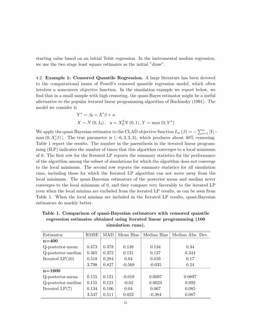
Table 1 report the results. The number in the parenthesis in the iterated linear program-ming (ILP) indicates the number of times that this algorithm converges to a local minimumof 0. The first row for the Iterated LP reports the summary statistics for the performanceof the algorithm among the subset of simulations for which the algorithm does not convergeto the local minimum. The second row reports the summary statistics for all simulationruns, including those for which the Iterated LP algorithm can not move away from thelocal minimum. The quasi-Bayesian estimators of the posterior mean and median neverconverges to the local minimum of 0, and they compare very favorably to the iterated LPeven when the local minima are excluded from the iterated LP results, as can be seen fromTable 1. When the local minima are included in the Iterated LP results, quasi-Bayesianestimators do markly better.

Table 1. Comparison of quasi-Bayesian estimators with censored quantileregression estimates obtained using iterated linear programming (100

simulation runs).

Estimator RMSE MAD Mean Bias Median Bias Median Abs. Dev.n=400Q-posterior-mean 0.473 0.378 0.138 0.134 0.34Q-posterior-median 0.465 0.372 0.131 0.137 0.344Iterated LP(10) 0.518 0.284 0.04 0.016 0.17

3.798 0.827 -0.568 -0.035 0.24n=1600Q-posterior-mean 0.155 0.121 -0.018 0.0097 0.0897Q-posterior-median 0.155 0.121 -0.02 0.0023 0.092Iterated LP(7) 0.134 0.106 0.04 0.067 0.085

3.547 0.511 0.023 -0.384 0.087

21

4.3. Example 2: Instrumental Median Regression. We consider a simulation examplesimilar to that in Koenker (1994). The model is

Y = D′β0 + u, u = σ(D)ε,

D = expN(0, I3), ε = N(0, 1), σ(D) = (1 + P3i=1D(i))/5.

The true parameter β0 equals 0, and we consider the instrumental moment conditions

gn(θ) =1n

n∑

i=1

(12− 1(Yi ≤ α + D′β))Z, where Z = (1, D).

The weight matrix is given by W =[

14n

∑ni=1 ZiZ

′i

]−1. While instrumental median regres-

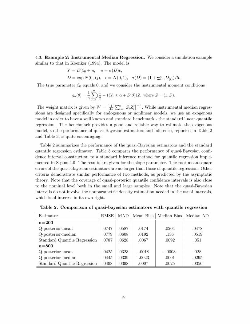
sions are designed specifically for endogenous or nonlinear models, we use an exogenousmodel in order to have a well known and standard benchmark - the standard linear quantileregression. The benchmark provides a good and reliable way to estimate the exogenousmodel, so the performance of quasi-Bayesian estimators and inference, reported in Table 2and Table 3, is quite encouraging.

Table 2 summarizes the performance of the quasi-Bayesian estimators and the standardquantile regression estimator. Table 3 compares the performance of quasi-Bayesian confi-dence interval construction to a standard inference method for quantile regression imple-mented in S-plus 4.0. The results are given for the slope parameter. The root mean squareerrors of the quasi-Bayesian estimators are no larger than those of quantile regression. Othercriteria demonstrate similar performance of two methods, as predicted by the asymptotictheory. Note that the coverage of quasi-posterior quantile confidence intervals is also closeto the nominal level both in the small and large samples. Note that the quasi-Bayesianintervals do not involve the nonparametric density estimation needed in the usual intervals,which is of interest in its own right.

Table 2. Comparison of quasi-bayesian estimators with quantile regression

Estimator RMSE MAD Mean Bias Median Bias Median AD

n=200Q-posterior-mean .0747 .0587 .0174 .0204 .0478Q-posterior-median .0779 .0608 .0192 .136 .0519Standard Quantile Regression .0787 .0628 .0067 .0092 .051n=800Q-posterior-mean .0425 .0323 -.0018 -.0003 .028Q-posterior-median .0445 .0339 -.0023 .0001 .0295Standard Quantile Regression .0498 .0398 .0007 .0025 .0356

22

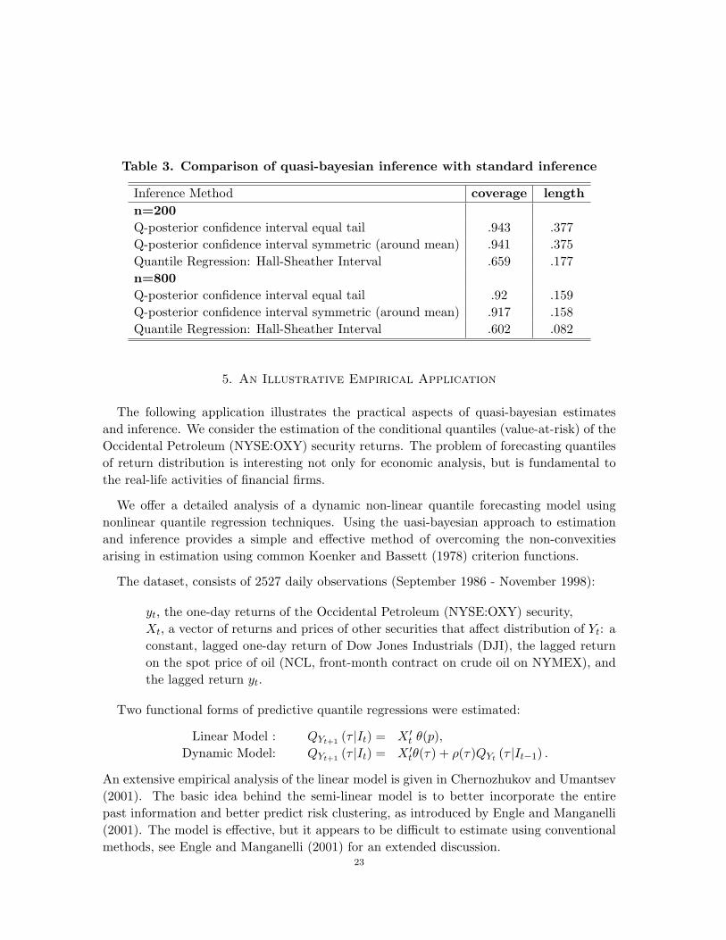
Table 3. Comparison of quasi-bayesian inference with standard inference

Inference Method coverage lengthn=200Q-posterior confidence interval equal tail .943 .377Q-posterior confidence interval symmetric (around mean) .941 .375Quantile Regression: Hall-Sheather Interval .659 .177n=800Q-posterior confidence interval equal tail .92 .159Q-posterior confidence interval symmetric (around mean) .917 .158Quantile Regression: Hall-Sheather Interval .602 .082

5. An Illustrative Empirical Application

The following application illustrates the practical aspects of quasi-bayesian estimatesand inference. We consider the estimation of the conditional quantiles (value-at-risk) of theOccidental Petroleum (NYSE:OXY) security returns. The problem of forecasting quantilesof return distribution is interesting not only for economic analysis, but is fundamental tothe real-life activities of financial firms.

We offer a detailed analysis of a dynamic non-linear quantile forecasting model usingnonlinear quantile regression techniques. Using the uasi-bayesian approach to estimationand inference provides a simple and effective method of overcoming the non-convexitiesarising in estimation using common Koenker and Bassett (1978) criterion functions.

The dataset, consists of 2527 daily observations (September 1986 - November 1998):

yt, the one-day returns of the Occidental Petroleum (NYSE:OXY) security,Xt, a vector of returns and prices of other securities that affect distribution of Yt: aconstant, lagged one-day return of Dow Jones Industrials (DJI), the lagged returnon the spot price of oil (NCL, front-month contract on crude oil on NYMEX), andthe lagged return yt.

Two functional forms of predictive quantile regressions were estimated:

Linear Model : QYt+1 (τ |It) = X ′t θ(p),

Dynamic Model: QYt+1 (τ |It) = X ′tθ(τ) + ρ(τ)QYt (τ |It−1) .

An extensive empirical analysis of the linear model is given in Chernozhukov and Umantsev(2001). The basic idea behind the semi-linear model is to better incorporate the entirepast information and better predict risk clustering, as introduced by Engle and Manganelli(2001). The model is effective, but it appears to be difficult to estimate using conventionalmethods, see Engle and Manganelli (2001) for an extended discussion.

23

The quasi-bayesian estimation and inference strategy is based on the Koenker and Bassett(1978) criterion function: (qt(τ ; θ, ρ) = QYt+1 (τ |It))

Qn(θ, ρ) =n∑

t=s

wt(τ)ρτ (Yt − qt(τ ; θ, ρ)),

where in the first step the estimates are constructed using wt(τ) = 1/τ(1−τ), and then theinitial estimates are used to construct the weights wt(τ) = (h/(qt(τ + h)− qt(h)) /τ(1− τ)where h ∝ Cn−1/3 and C > 0 is chosen using Hall-Sheather rule, see Koenker (1994).Using such weights we achieve the generalized information matrix equality needed to usethe quasi-posterior quantiles for inference purposes.

Figure 2 presents surfaces of the regression VaR functions of the dynamic semi-linearmode plotted in the time-probability level coordinates, (t, τ). Recall that τ is the quantileindex. We report V aR for values of τ ∈ [.2, .8]. The conventional V aR reporting typicallyinvolves the probability levels at a given τ . Clearly, the whole VaR surface formed byvarying τ represents a more complete depiction of conditional risk. We also present theVaR surface for the static linear model in figure 3.

The dynamics depicted in Figures 2 and 3 unambiguously indicates certain dates on whichmarket risk tends to be much higher than its usual level. This by itself underscores theimportance of conditional modeling. The driving force behind the dynamics is the behaviorof Xt. The static model indicates somewhat lower VaR at the lower quantile range.

Finally, we focus on the dynamic semi-linear model and provide the economic interpre-tation of the slope coefficient functions θ2(·), θ3(·), θ4(·), θ5 (·), corresponding to the laggedreturns on oil spot price, X2, the equity index, X3, the price of the security in question,X4, and the lagged VaR, X5.

θ2(·) is insignificantly positive in the left and right quantiles of the distribution of yt

conditional on Xt. It is insignificantly negative in the middle part. θ3(·), in contrast, issignificantly positive for all values of τ . with the possible exception of the far right tailof yt conditional on Xt. We also notice a sharp increase in the middle range. Thus, inaddition to the strong positive relation between the stock return on the individual stockand the market return (DJI) (dictated by the fact that θ2(·) > 0 on (0.2, 0.8)) there is alsoadditional sensitivity of the median of the security return to the market movements. Forlow positive returns, in contrast, the market return has a much weaker effect (low valueson (0.2)).

θ4(·), in contrast, is significantly negative, except for values of p close to 0. This maybe clearly interpreted as a mean reversion effect in the central part of the distribution.However, X3, the lagged return, does not appear to significantly shift the quantile functionin the tails. Thus, X3 is more important for the determination of intermediate risks.

24

Interestingly, ρ (·), the dynamic coefficient on the lagged VaR is significantly negative inthe low quantiles and in the high quantiles, but is insignificant in the middle range. Thesignificance of ρ (·) provides strong evidence against the non-recursive linear specification.This indicates both a ”mean reversion” and significant risk clustering effect in the tails ofthe distribution(see Figure 7). As expected, there does not appear to be much of an effectover the median range, which is consistent with random walk properties of the stock price.Thus the dynamic effect of lagged VaR is much more important for the tails of the quantilefunction, which is important for risk managements.

6. Conclusion

In this paper, we study the properties of a class of quasi-Bayesian estimators that aredefined using common econometric, non-likelihood based functions. We showed that un-der regularity conditions these estimators are

√n consistent and asymptotically normal,

and quasi-posterior quantiles provide asymptotically valid confidence intervals. A simula-tion study illustrates the finite sample properties of the proposed estimation and inferencemethods. We apply them to an empirical example of nonlinear value at risk modelling. Itemerges from these results that in many important cases the quasi-Bayesian estimators canprovide useful alternatives to the usual optimization estimators. In ongoing work, we areextending the results to models in which

√n convergence rate and asymptotic normality do

not hold, including nonregular likelihood functions in Donald and Paarsch (1993), includingthe maximum score estimator of Manski (1975), and models in which the true parameter ison the boundary of the parameter space, e.g. Andrews (1999).

25

Appendix A

A.1. Proof of theorem 1. We need to show∫

Hn

|h|α∣∣∣p∗n(h)− p∗∞(h)

∣∣∣dhp−→ 0 (A.1)

for all α ≥ 0. Our arguments follow those in Bickel and Yahav (1969), as presented in Lehmannand Casella (1998). As indicated in the text, the main difference appears in part 2, and are due tothe non-likelihood setting and the use of Huber-like conditions 4.iv to handle discontinuous criterionfunctions. We also handle non-symmetric loss functions. The results obtained in part 1 are similarto the result on p.489-490 in Lehmann and Casella (1998), except that we are showing a strongerresult needed to go beyond posterior means. Throughout this proof the range of integration for h isgiven by Hn.

Part 1. We defined h =√

n (θ − θ0)−J (θ0)−1 ∆n (θ0) /

√n, and Tn = θ0 + 1

nJ (θ0)−1 ∆n (θ0), then

p∗n (h) =π

(h√n

+ Tn

)exp

(Ln

(h√n

+ Tn

))

∫Hn

π(

h√n

+ Tn

)exp

(Ln

(h√n

+ Tn

))dh

=π

(h√n

+ Tn

)exp (ω(h))

∫Hn

π(

h√n

+ Tn

)exp (ω(h)) dh

≡π

(h√n

+ Tn

)exp (ω(h))

Cn

where

ω (h) = Ln

(Tn +

h√n

)− L (θ0)− 1

2n∆n (θ0)

′J (θ0)

−1 ∆n (θ0)

and

Cn ≡∫

Hn

π

(h√n

+ Tn

)exp (ω (h)) dh.

In part 2 we will show that for each α ≥ 0,

J1 ≡∫

Hn

|h|α∣∣∣∣ exp (w (h))π

(Tn +

h√n

)− exp

(−1

2h′J (θ0) h

)π (θ0)

∣∣∣∣dhp−→ 0. (A.2)

Given (A.2), then taking the case α = 0 we have

Cnp−→

∫

Rd

e−12 h′J(θ0)hπ (θ0) dh = π (θ0) (2π)

d2|J (θ0) |1/2. (A.3)

Next note that∫

Hn

|h|α∣∣∣∣p∗n (h)− p∗∞ (h)

∣∣∣∣dh = J · C−1n ,

26

where

J ≡∫

Hn

|h|α∣∣∣∣ew(h)π

(Tn +

h√n

)− (2π)−d/2|J (θ0) |1/2 exp

(−1

2h′J (θ0) h

)· Cn

∣∣∣∣dh

Using (A.3), it suffices to show that Jp−→ 0, but

J ≤ J1 + J2,

where

J1p−→ 0,

by (A.2) and

J2 =∫

Hn

|h|α∣∣∣∣Cn(2π)−d/2|J (θ0) |1/2 exp

(−1

2h′J (θ0)h

)− π (θ0) exp

(−1

2h′J (θ0)h

) ∣∣∣∣dh

=∣∣∣∣Cn(2π)−d/2|J (θ0) |1/2 − π (θ0)

∣∣∣∣∫

Hn

|h|α exp(−1

2h′J (θ0)h

)dh

p−→ 0.

Part 2. It remains only to show (A.2). Given assumption 4 we can write

ω (h) = −12h′J (θ0)h−Rn(

h√n

+ Tn)

We consider the integral J1 in (A.2) in three seperate areas:

• Area (i) : |h| ≤ M ,• Area (ii) : M ≤ |h| ≤ δ

√n,

• Area (iii) : |h| ≥ δ√

n.

Each of these areas is implicitly understood to intersect with the range of integration for h, whichis Hn.

Area (i): We will show that for each 0 < M < ∞, and each ε > 0,

lim infn

P

∫

|h|≤M

|h|α∣∣∣∣ exp (w (h))π

(Tn +

h√n

)

− exp(−1

2h′J (θ0)h

)π (θ0)

∣∣∣∣dh < ε

≥ 1− ε.

(A.4)

This is proved by showing that

sup|h|≤M

|h|α∣∣∣∣ exp (w (h))π

(Tn +

h√n

)− exp

(−1

2h′J (θ0) h

)π (θ0)

∣∣∣∣p−→ 0 (A.5)

Using the expression for ω (h), (A.5) follows from:

(a) sup|h|≤M

∣∣∣∣π(

h√n

+ Tn

)− π (θ0)

∣∣∣∣p−→ 0,

(b) sup|h|≤M

∣∣∣∣Rn

(h√n

+ Tn

) ∣∣∣∣p−→ 0,

27

where (a) follows obviously from the continuity of π (·) and because by assumption 4.ii-4.iii:

1√n

J (θ0)−1 ∆n (θ0) = Op (1) (A.6)

Given (A.6), (b) follows from assumption 4.(iv), since (A.6) implies that

sup|h|≤M

∣∣∣∣Tn +h√n− θ0

∣∣∣∣ = Op(1/√

n).

Area (ii): We show that that for each ε > 0 there exist large M and small δ > 0 such that

lim infn

P

∫

M<|h|<δ√

n

|h|α∣∣∣∣ exp (w (h))π

(Tn +

h√n

)

− exp(−1

2h′J (θ0)h

)π (θ0)

∣∣∣∣dh < ε

≥ 1− ε

(A.7)

Since the second term of the integrand is integrable, it suffices to show this for the first term of theintegrand. In order to show this it will suffice to show that for sufficiently large M as n → ∞, thefirst term is integrable with probability greater than 1− ε,

exp (w (h)) π

(Tn +

h√n

)≤ C exp

(−1

4h′J (θ0)h

), for all M < |h| < δ

√n. (A.8)

By assumption π (·) < K, so we can drop it from consideration.

By definition of ω(h)

exp (w (h)) ≤ exp

(− 1

2h′J (θ0)h +

∣∣∣∣Rn

(Tn +

h√n

) ∣∣∣∣)

Since |Tn − θ0| = op(1), we have wp → 1, for any δ > 0,∣∣∣∣Tn +

h√n− θ0

∣∣∣∣ < 2δ, for all |t| ≤ δ√

n.

Thus, by assumption 4.iv(a) there exists some small δ and large M

P

sup

M≤|h|≤δ√

n

|Rn

(Tn + h√

n

)|

|h + 1√nJ (θ0)

−1 ∆n (θ0) |2≤ 1

4mineig (J (θ0))

≥ 1− ε.

Since 1n

∣∣J (θ0)−1 ∆n (θ0)

∣∣2 = Op (1) we obtain for some C > 0,

P

exp (w (h)) ≤ C exp

(−1

4h′J (θ0) h

)

≥ P

ew(h) ≤ C exp

(−1

2h′J (θ0)h +

14mineig (J (θ0)) |h|2

) ≥ 1− ε.

(A.9)

(A.9) implies (A.8), which in turn implies (A.7).28

Area (iii): We show that for each ε > 0 and each δ > 0,

lim infn

P

∫

h≥δ√

n

|h|α∣∣∣∣ exp (w (h))π

(Tn +

h√n

)

− exp(−1

2h′J (θ0)h

)π (θ0)

∣∣∣∣dh < ε

≥ 1− ε.

(A.10)

The second integrand obviously goes to 0 as n → ∞, due to integrability. Therefore we only needto show ∫

|h|≥δ√

n

|h|αeω(h)π

(Tn +

h√n

)dh →p 0.

Recalling the definition of h, the term is bounded by

√n

α+1∫

|θ−Tn|≥δ

∣∣∣∣Tn − θ

∣∣∣∣α

π (θ) exp(

Ln (θ)− Ln (θ0)− 12n

∆n (θ0)′J (θ0)

−1 ∆n (θ0))

dθ.

Since Tn − θ0p−→ 0, wp → 1 this is bounded by

Kn · C · √nα+1

∫

|θ−θ0|≥δ/2

(1 +

∣∣θ∣∣α)

π (θ) exp (Ln (θ)− Ln (θ0)) dθ.

where

Kn = exp(− 1

2n∆n (θ0)

′J (θ0)

−1 ∆ (θ0))

= Op (1) .

By Assumption 3 there exists ε > 0 such that

lim infn→∞

P

sup

|θ−θ0|≥δ/2

eLn(θ)−Ln(θ0) ≤ e−nε

= 1

Thus wp → 1 the entire term is bounded by:

Kn · C · √nα+1 · e−nε

∫

Θ

|θ|απ (θ) dθ = op(1).

The proof is completed by combining statements in equations (A.4), (A.7), and (A.10). ¥

A.2. Proof of theorem 2. Recall that

h =√

n (θ − θ0)− J (θ0)−1 ∆n (θ0) /

√n.

Define Wn = J(θ0)−1∆n(θ0)/√

n. Consider the objective function

Qn(z) =∫

Hn

ρ(z − h−Wn)p∗n(h)dh,

which is minimized by z =√

n(θ − θ0). Also define

Q∞(z) =∫

Rd

ρ(z − h−Wn)p∗∞(h)dh.

29

which is minimized at Zn. Define

ξ = arg minz∈Rd

[∫

Rd

ρ(z − h)p∗∞(h)dh.

]

Note that solution is unique and finite by assumption 2 parts (ii) and (iii) on the loss function ρ.When ρ is symmetric the solution ξ = 0 by Anderson’s lemma(see van der Vaart (1999)).

Therefore, Zn = arg minz∈Rd Q∞(z) equals

Zn = ξ + Wn = Op(1).

Next, we have for any finite k,

(Qn(zj), j ≤ k)− (Q∞(zj), j ≤ k) →p 0

since by assumption 2.(ii) ρ(h) ≤ 1 + |h|p, and because |a + b|p ≤ 2p−1|a|p + 2p−1|b|p for p ≥ 1,

|Qn(z)−Q∞(z)| ≤∫

Hn

(1 + |z − h−Wn|p) |p∗n(h)− p∗∞(h)|dh

+∫

Hcn

(1 + |z − h−Wn|p) (p∗∞(h)) dh

≤∫

Hn

(1 + 2p−1|h|p + 2p−1|z −Wn|p

) |p∗n(h)− p∗∞(h)|dh

+∫

Hcn

(1 + 2p−1|h|p + 2p−1|z −Wn|p

)(p∗∞(h)) dh

≤∫

Hn

(1 + 2p−1|h|p + Op(1)

)(p∗n(h)− p∗∞(h)) dh

+∫

Hcn

(1 + 2p−1|h|p + Op(1)

)(p∗∞(h)) dh = op(1),

where op(1)-conclusion is by Theorem 1 and exponentially small tails of the normal density (Lebesguemeasure of Hc

n converges to zero).

Now note that Qn(z), Q∞(z), are convex and finite, and Zn = arg minz∈Rd Q∞(z) = Op(1). Bythe convexity lemmas of Rockafellar and Wets (1998), Knight (1999) and Pollard (1991), pointwiseconvergence entails the uniform convergence over compact sets K:

supz∈K

∣∣∣Qn(z)−Q∞(z)∣∣∣ →p 0.

Since Zn = Op(1), uniform convergence and convexity arguments imply that√

n(θ− θ0)−Zn →p 0,as shown below. ¥

Proof of Zn−√

n(θ−θ0) = op(1). The proof follows by extending slightly the convexity argumentof Jureckova (1977) to the present context. Consider a ball Bδ (Zn) with radius δ > 0, centeredat Zn, and let z = Zn + δv, where v is a unit direction vector s.t. |v| = 1 and |d| > δ. BecauseZn = Op(1), for any δ > 0 and ε > 0, there is large enough K > 0 such that Bδ (Zn) is contained insome ball BK(0) in the sense that

lim infn→∞

P En = Bδ (Zn) ∈ BK (0) ≥ 1− ε.

30

By convexity in z

δ

d

(Qn(z)−Qn(Zn)

) ≥ Qn(z∗)−Qn(Zn), (A.11)

where z∗ is a point of boundary of Bδ(0) on the line connecting z and Zn. By the inform convergenceof Qn (z) to Q∞ (z) over any compact set BK (0), whenever En occurs:

δ

d

(Qn(z)−Qn(Zn)

) ≥ Qn(z∗)−Qn(Zn)

≥ Q∞(z∗)−Q∞(Zn) + op(1) ≥ V + op(1),

where V > 0 is a positive random variable. Since V > 0 there is η > 0 such that P (V > η) ≥ 1− ε,we have with probability at least as big as 1− 3ε for large n:

δ

d

(Qn(z)−Qn(Zn)

)> η.

Thus√

n(θ − θ0) eventually belongs to a complement of Bδ (Zn) only with probability at most 3ε.We can set ε as small as we like by picking

(a) sufficiently large K,(b) sufficient large n,(c) sufficiently small η > 0,

it follows that

lim supn→∞

P|Zn −

√n

(θ − θ0

)|δ

= 0.

Since this is true for any δ > 0, it follows that

Zn −√

n(θ − θ0) = op(1). ¥

A.3. Proof of theorem 3. We defined

Fg,n(x) =∫

θ∈Θ:g(θ)≤x

pn(θ)dθ.

Evaluate it at x = g(θ0) + s/√

n and change the variable of integration

Hg,n(s) = Fg,n(g(θ0) + s/√

n) =∫

h:g(θ0+h/√

n+Wn/√

n)≤g(θ0)+s/√

n

p∗n(h)dh.

Define alsoHg,n(s) =

∫

h:g(θ0+h/√

n+Wn/√

n)≤g(θ0)+s/√

n

p∗∞(h)dh

andHg,∞(s) =

∫

h:∇g(θ0)′(h/√

n+Wn/√

n)≤s/√

n

p∗∞(h)dh.

By definition of total variation norm and Theorem 1

sups|Hg,n(s)− Hg,n(s)| ≤

∥∥∥p∗n − p∗∞∥∥∥

T V

→p 0.

By the uniform continuity of integral of the normal density with respect to the boundary of integra-tion

sups|Hg,n(s)−Hg,∞(s)| →p 0 implies sup

s|Hg,n(s)−Hg,∞(s)| →p 0.

31

Convergence of distribution function implies convergence of quantiles, see e.g. Billingsley (1994):

H−1g,n(α)−H−1

g,∞(α) →p 0.

Next observeHg,∞(s) = Pr(∇g(θ0)T N(Wn, J−1(θ0)) < s|Wn),

so thatH−1

g,∞(α) = ∇g(θ0)T Wn + qα

√∇θg(θ0)T J−1(θ0)∇θg(θ0),

where qα is the α-quantile of N(0, 1).

Recalling that we defined Qg,n(α) = F−1g,n(α), observe that by quantile equivariance with respect to

the monotone transformations H−1g,n(α) =

√n (Qg,n(α)− g(θ0)) , so that

√n (Qg,n(α)− g(θ0)) = ∇g(θ0)T Wn + qα

√∇θg(θ0)T J−1(θ0)∇θg(θ0) + op(1).

The proof is completed by the “delta-method” theorem. ¥

A.4. Proof of Proposition 1. Assumption 3 is directly implied by (3.1)-(3.3) and the uniformcontinuity of Emi (θ), as shown in Lemma 1. It remains only to verify Assumption 4.

Now define the identify

Ln (θ)− Ln (θ0) ≡−ngn (θ0)W (θ0) G (θ0)︸ ︷︷ ︸∆n(θ0)

′

(θ − θ0)

−12

(θ − θ0)′nG (θ0) W (θ0) G (θ0)

′︸ ︷︷ ︸

J(θ0)

(θ − θ0)

+Rn (θ) .

(A.12)

Next, given the definition of terms ∆n (θ0) and J (θ0), conditions i, ii, iii of Assumption 4 areimmediate from the conditions i-iii of Proposition 1. Condition iv. is verified as follows. Conditioniv. of Assumption 4 can be succinctly stated as:

∀ε > 0, ∀η > 0, ∃δ > 0, s.t. lim supn→∞

P

(sup

|θ−θ0|≤δ

|Rn (θ) |1 + n|θ − θ0|2 > ε

)< η.

This stochastic equi-continuity condition is equivalent to the following stochastic equi-continuitycondition, see e.g. Andrews (1994): for any δn −→ 0

sup|θ−θ0|≤δn

Rn (θ)1 + n|θ − θ0|2 = op (1) . (A.13)

This is weaker than condition (v) of Theorem 7.1 in Newey and McFadden (1994b), which requires

sup|θ−θ0|≤δn

Rn (θ)√n|θ − θ0|+ n|θ − θ0|2 = op (1) . (A.14)

To see this note that

Rn (θ)1 + n|θ − θ0|2 =

Rn (θ)√n|θ − θ0|+ n|θ − θ0|2

√n|θ − θ0|+ n|θ − θ0|2

1 + n|θ − θ0|2 ,

32

with the second term bounded by

1 +√

n|θ − θ0|1 + n|θ − θ0|2 ≤ 1 +

1√n|θ − θ0|+ 1√

n|θ−θ0|≤ 2.

Therefore, to show the requisite condition, we will verify either the condition (A.13) or (A.14).The arguments of the proof, apart from several important differences, follow those of theorem 7.2in Newey and McFadden (1994b).

At first note that condition iv. of Proposition 1 is implied by the condition (where we letg (θ) ≡ Egn (θ)):

supθ∈Bδn (θ0)

ε (θ) = op

(1√n

), where ε (θ) =

gn (θ)− gn (θ0)− g (θ)1 +

√n|θ − θ0| and δn → 0. (A.15)

From (A.12), the reminder term Rn (θ) = R1n (θ) + R2n (θ) + R3n (θ), where is

R1n (θ) ≡− n

(−gn (θ0)

′W (θ)G (θ0) (θ − θ0)− 1

2(θ − θ0)

′G (θ0)

′W (θ) G (θ0) (θ − θ0)

− 12gn (θ)′Wn (θ) gn (θ) +

12gn (θ0)

′Wn (θ) g (θ0)

),

R2n (θ) ≡− n

(12gn (θ0)

′ (Wn (θ0)−Wn (θ)) gn (θ0))

,

R3n (θ) ≡− n

(gn (θ0)

′ (W (θ)−W (θ0))G (θ0) (θ − θ0)

+12

(θ − θ0)′G (θ0)

′ (W (θ)−W (θ0))G (θ0) (θ − θ0))

Verification of (A.14) for the term R3n (θ) is immediate and follows from the continuity of W (θ)in θ by condition i. of Proposition 1, so that W (θ) −W (θ0) = o (1) as |θ − θ0| → 0. Verificationof (A.14) for the term R2n (θ) is immediate and follows from the uniform consistency of Wn (θ) in θ

as assumed in condition i. of Proposition 1 and from the continuity of W (θ) in θ by condition i. ofProposition 1, so that Wn (θ)−W (θ) = op (1) uniformly in θ and from W (θ)−W (θ0) = op (1) as|θ − θ0| → 0.

It remains to check the condition (A.14) for the term R1n (θ). Note that

gn (θ) =(1 +

√n|θ − θ0|

)ε (θ) + g (θ) + gn (θ0) .

33

substitute this into R1n (θ) and decompose

− 1n

R1n (θ) =12

(1 +

√n|θ − θ0|

)2ε (θ)′Wn (θ) ε (θ)

︸ ︷︷ ︸r1(θ)

+ gn (θ0)′Wn (θ) (g (θ)−G (θ0) (θ − θ0))︸ ︷︷ ︸

r2(θ)

+(1 +

√n|θ − θ0|

)ε (θ)′Wn (θ) gn (θ0)︸ ︷︷ ︸

r3(θ)

+(1 +

√n|θ − θ0|

)ε (θ)′Wn (θ) g (θ)︸ ︷︷ ︸

r4(θ)

+12g (θ)′ (Wn (θ)−W (θ)) g (θ)

︸ ︷︷ ︸r5(θ)

+12g (θ)′W (θ) g (θ)− 1

2(θ − θ0)

′G (θ0)

′W (θ)G (θ0) (θ − θ0)

︸ ︷︷ ︸r6(θ)

.

Using the algebraic relations, for x ≥ 0:

(1 +√

nx)2

1 + nx2≤ 2,

√nx

1 + nx2≤ 1,

1 +√

nx

1 + nx2≤ 2,

n (1 +√

nx)1 + nx2

≤ 2√

n

x, (A.16)

each of these terms can be dealt with separately, by applying the conditions i.-iii. and (A.15):

(a) supθ∈Bδn (θ0)

nr1 (θ)1 + n|θ − θ0|2 ≤ sup

θ∈Bδn (θ0)

nε (θ)′Wn (θ) ε (θ) = op (1) ,

(b) supθ∈Bδn (θ0)

nr2 (θ)1 + n|θ − θ0|2 = sup

θ∈Bδn (θ0)

o (n|θ − θ0|)′Wn (θ) gn (θ0)1 + n|θ − θ0|2 = op (1) ,

(c) supθ∈Bδn (θ0)

nr3 (θ)1 + n|θ − θ0|2 ≤ sup

θ∈Bδn (θ0)

2nε (θ)′Wn (θ) gn (θ0) = op (1)

(d) supθ∈Bδn (θ0)

nr4 (θ)1 + n|θ − θ0|2 ≤ sup

θ∈Bδn (θ0)

2√

n

∣∣∣∣ε (θ)′Wn (θ)|g (θ) ||θ − θ0|

∣∣∣∣ = op (1) ,

(e) supθ∈Bδn (θ0)

nr5 (θ)1 + n|θ − θ0|2 ≤ sup

θ∈Bδn (θ0)

|g (θ) |2|θ − θ0|2 |Wn (θ)−W (θ) | = op (1) ,

(f) supθ∈Bδn (θ0)

nr6 (θ)1 + n|θ − θ0|2 ≤ sup

θ∈Bδn (θ0)

o(|θ − θ0|2|W (θ) |)

|θ − θ0|2 = o (1) ,

where (a) follows from (A.16), (A.15), and condition i. that states that Wn (θ) = W (θ) + op (1)and W (θ) > 0 both uniformly in θ; (b) follows from (A.16) and condition iii.; (c) follows from(A.16), (A.15), condition i. and iii.; (d) follows by (A.16) and then replacing by condition ii.g (θ) with G (θ0) (θ − θ0) + o (|θ − θ0|), followed by applying (A.15) and condition i.; (e) followsfrom (A.16) and then replacing by condition ii. g (θ) with G (θ0) (θ − θ0) + o (|θ − θ0|), followed byapplying condition i.; and (f) follows from replacing g (θ) with G (θ0) (θ − θ0)+ o (|θ − θ0|), followedby applying condition i.

Verification of (A.14) for the term R1n (θ) now follows by putting these terms together. ¥

A.5. Proof of Proposition 2. Verification of Assumption 3 is standard given the stated conditionsand is subsumed as a step in the consistency proofs of extremum estimators based on GEL inKitamura and Stutzer (1997) or cases when s is finite and Kitamura (1997) for cases when s takeson infinite values. Therefore, it shall not be repeated here. Next, we will verify Assumption 4.

34

Define

γ (θ) = arg minγ∈Rp

Ln (θ, γ) .

It will suffice to show that uniformly in θ ∈ Bδn(θ0) for any δn → 0, we have the GMM set-up:

Ln (θn) =Ln (θn, γ (θn))

=− 12

(1√n

n∑

i=1

mi (θn)

)′

(V (θ0) + op (1))−1

(1√n

n∑

i=1

mi (θn)

),

(A.17)

where

V (θ0) = Emi (θ0)mi (θ0)′

The Assumption 4.i-iii is immediate from the conditions of Proposition 2, and the Assumption 4.ivis verified exactly as in the proof of Proposition 1 given the reduction to the GMM case. Indeed,defining gn (θ) = 1

n

∑ni=1 mi (θ), the Donsker property assumed in condition iv. implies that for any

ε > 0, there is δ > 0 such that

lim supn→∞

P

sup

θ∈Bδn(θ0)

√n|gn (θ)−Gn (θ0)− (Egn (θ)− Egn (θ0)) | > ε

< ε,

which implies

lim supn→∞

P

sup

θ∈Bδn(θ0)

√n|gn (θ)−Gn (θ0)− (Egn (θ)− Egn (θ0)) |

1 +√

n|θ − θ0| > ε

< ε,

which is the condition iv. in Proposition 1. The rest of the arguments follow that in the proof ofProposition 1.

It only remains to show the requisite expansion (A.17). At first, we show that

γ (θn) →p 0.

For that purpose we use the convexity lemma, which was obtained by C. Geyer, and can be foundin Knight (1999).

Convexity Lemma. Suppose Qn is a sequence of lower-semi-continuous convex R-valued randomfunctions, defined on Rd, and let D be a countable dense subset of Rd. If Qn converges to Q∞ in Rmarginally (in finite-dimensional sense) on D where Q∞ is lower-semi-continuous convex and finiteon an open non-empty set a.s., then

arg minz∈Rd

Qn (z) →d arg minz∈Rd

Q∞ (z) ,

provided that the latter is uniquely defined a.s. in Rd.

To show γ (θn) →p 0, note that γ ∈ F = γ : Es[mi (θ0)

′γ]

< ∞ or γ ∈ F c = γ :Es

[mi (θ0)

′γ]

= ∞. By convexity and lower-semi-continuity of s, F is convex, open, and itsboundary is nowhere dense in Rp. Thus for γ ∈ F , Es

[mi (θ)′ γ

]< ∞, wp → 1, once θ ∈ Bδ (θ0)

for sufficiently small δ > 0, by continuity of θ → Es[mi (θ)′ γ

]over Bδ (θ0) implied by conditions

ii. and iii.35

Thus, for an given γ ∈ F

1n

n∑

i=1

s[mi (θn)′ γ

] →p Es[mi (θ0)

′γ]

< ∞.

This follows from the uniform law of large numbers implied by

1. s[mi (θ)′ γ], θ ∈ Bδ (θ0), where δ > 0 is sufficiently small, being a Donsker class wp → 1,

2. Emi (θ) =∫

xdP [mi (θ) ≤ x] being continuously differentiable in θ by condition ii. and iii.

The above set is Donsker by

(a) s being uniform Lipshitz function over V ∩M where M is compact, by assumption on s,(b) for δ > 0 small, mi (θ)′ γ ∈ V for all θ ∈ Bδ (θ0) for a given γ ∈ F by construction of F ,(c) mi (θ)′ γ ∈ M for some compact M , for a given γ ∈ F , by condition iii.(d) mi (θ) , θ ∈ Bδ (θ0) being Donsker by condition iv.,(e) Theorem 2.10.6 in Van der Vaart and Wellner (1996) that says a uniform Lipschitz trans-

formation of a Donsker class is Donsker class itself.

Now take γ ∈ F c \ ∂F , where ∂F denotes the boundary of F . Then wp → 1

1n

n∑

i=1

s[mi (θn)′ γ

]= ∞→p Es

[mi (θ0)

′γ]

= ∞.

Now take all the rational numbers γ ∈ Rp \ ∂F as the set D appearing in the statement of theConvexity lemma and conclude that

γ (θn) →p 0 = arg infγ

Es[mi (θ0)

′γ].

Given this result, we can expand the first order condition for γ (θn) in order to obtain the expres-sion for its form. Note first

0 =n∑

i=1

∇s(γ (θn)′mi (θn)

)mi (θn)

=n∑

i=1

mi (θn) + γ (θn)nVn,

where

Vn =1n

n∑

i=1

∇2s(γ (θn)′mi (θn)

)mi (θn) mi (θn)′ ,

for some γ (θn) between 0 and γ (θn), which is different from row to row of the matrix Jn.

ThenVn →p V (θ0) = Emi (θ0)mi (θ0)

′.

This follows from the uniform law of large numbers implied by

1. ∇2s (γ′mi (θ∗)) mi (θ) mi (θ)′ , (θ∗, γ, θ) ∈ Bδ1 (θ0) × Bδ2 (0) × Bδ3 (θ0), where δj > 0 aresufficiently small, being a Donsker class wp → 1,

36

2. Emi (θ)mi (θ)′ =∫

xx′dP [mi (θ) ≤ x] being continuous function in θ by condition i.,

3. E∇2s (γ′mi (θ∗)) mi (θ) mi (θ)′ = E∇2s (0)︸ ︷︷ ︸1

mi (θ)mi (θ)′+o (1) uniformly in (θ, θ∗) ∈ Bδ (θ0)×

Bδ (θ0) for sufficiently small δ > 0, for any γ → 0, by assumptions on s and condition iii.

Then claim 1 is verified by applying exactly the same logic as in the previously stated steps (a)-(e).For brevity, this will not be repeated.

Therefore, wp → 1

γ (θn) = − (Vn)−1 1n

n∑

i=1

mi (θn) ≡ −(V (θ0)

−1 + op (1)) 1

n

n∑

i=1

mi (θn) . (A.18)

Consider the second order expansion

Ln (θn, γ (θn)) =√

nγ (θn)′1√n

n∑

i=1

mi (θ0) +12√

nγ (θn)′ Vnγ (θn) , (A.19)

where

Vn =1n

n∑

i=1

∇2s(γ (θn)′mi (θn)

)mi (θn) mi (θn)′ ,

for some γ (θn) between 0 and γ (θn), which is different from row to row of the matrix Vn. By apreceding argument,

Vn →p V (θ0) .

Inserting (A.18) and Vn = V (θ0)+op (1), into the expansion (A.19), we obtain the required expansion(A.17). ¥

A.6. Proof of Proposition 3. Assumption 3 is assumed. We need to verify Assumption 4.

Define the identity

Ln (θ)− Ln (θ0) ≡n∑

i=1

m (θ0)′

︸ ︷︷ ︸∆n(θ0)

′

(θ − θ0)

−12

(θ − θ0)′n∇θθ′Emi (θ0)︸ ︷︷ ︸

J(θ0)

(θ − θ0)

+Rn (θ) .

(A.20)

Assumption 4.i-iii then follows immediately from conditions ii. and iii.. Assumption 4.iv is verifiedas follows.

37

The remainder term Rn (θ) is given by the following decomposition:

Rn (θ) =n∑

i=1

mi(θ)−mi(θ0)− Emi(θ) + Emi(θ0)− mi(θ0)′(θ − θ0)

︸ ︷︷ ︸R1n(θ)

+ n (Emi(θ)− Emi(θ0))− (θ − θ0)′nJ(θ0)(θ − θ0)︸ ︷︷ ︸R2n(θ)

It suffices to verify assumption 4.iv separately for R1n(θ) and R2n(θ). Since

R2n(θ) = n(θ − θ0)′ [J(θ∗)− J(θ0)] (θ − θ0),

for some θ∗ on the line connecting θ and θ0, verification of Assumption 4 for R2n (θ) follows imme-diately from continuity of J (θ) in θ over a ball at θ0.

To show assumption 4.iv-(b) for R1n(θ), we note that for any given M > 0

lim supn

P ∗

sup|θ−θ0|≤M/

√n

|R1n (θ) | > ε

≤ lim supn

P

sup

|θ−θ0|≤M/√

n

|θ − θ0| |R1n (θ) ||θ − θ0| > ε

≤ lim supn

P

sup

|θ−θ0|≤M/√

n

M√n

|R1n (θ) ||θ − θ0| > ε

= 0,

(A.21)

where the last conclusion follows from two observations.

First, note that

Zn(θ) ≡ R1n (θ)√n|θ − θ0| = Gn

(mi(θ)−mi(θ0)− mi(θ0)′(θ − θ0)

|θ − θ0|)

is Donkser by assumption, that is it converges in `∞(Bδ(θ0)) to a tight Gaussian process Z. Theprocess has a uniformly continuous paths with respect to the semimetric ρ given by

ρ2(θ1, θ2) = E(Z(θ1)− Z(θ2))2,

such that ρ(θ, θ) → 0 if θ → θ0. Thus almost all sample paths of Z are continuous at θ0.

Second, by assumption since

E[mi(θ)−mi(θ0)− mi(θ0)′(θ − θ0)]2 = o(|θ − θ0|2),we have for any constant θn → θ0

E

[ |R1n (θn) |√n|θn − θ0|

]2

=o(|θn − θ|2)

|θn − θ0|2 → 0,

thereforeZ(θ0) = 0.

Therefore for any θ′ →p θ0, we have by extended continuous mapping theorem

Zn(θ′) →d Z(θ0) = 0, that is Zn(θ′) →p 0. (A.22)

This shows (A.21).38

To show assumption 4.iv-(a) for R1n(θ), we need to show that for some δ > 0 and constant M

lim supn

P ∗

supM/

√n≤|θ−θ0|≤δ

|R1n (θ) |n|θ − θ0|2 > ε

< ε, (A.23)

Bound the left hand side by, using that M/√

n ≤ |θ − θ0|

lim supn

P ∗

supM/

√n≤|θ−θ0|≤δ

|R1n (θ) |√n|θ − θ0| ·

1√n|θ − θ0| > ε

≤ lim supn

P ∗

supM/

√n≤|θ−θ0|≤δ

|R1n (θ) |√n|θ − θ0| ·

1M

> ε

≤ lim supn

P ∗

supM/

√n≤|θ−θ0|≤δ

|Zn(θ)| · 1M

> ε

< ε,

(A.24)

where for any given ε > 0 in order to make the last inequality true, we can make either δ sufficientlysmall by the property (A.22) of Zn or make M sufficiently large by the property Zn = Op∗(1). ¥.

Appendix B. Computation

B.1. A computational lemma. In this section we record some formal results on MCMC compu-tation of the quasi-posterior quantities.

Lemma 3. Suppose the chain (θ(j), j ≤ T ) is produced by the Metropolis Hastings(MH) algorithmwith q such that q(θ|θ′) > 0 for each (θ, θ′). Suppose also that Pρ(θ(j), ξ) = 1 > 0 for all j > t0.Then

(i) pn(·) is the stationary density of the chain,(ii) the chain is ergodic with the limit marginal distribution given by pn(·):

limT→∞

supA

∣∣∣P (θ(T ) ∈ A|θ0)−∫

A

pn(θ)dθ∣∣∣ = 0,

where the supremum is taken over the Borel sets,(iii) For any pn- integrable function g (·):

1T

T∑

j=1

g(θ(j)) →p

∫

Θ

g(θ)pn(θ)dθ.

Proof. See Robert and Casella (1999).

An immediate consequence of this lemma is the following result.

Lemma 4. Suppose Assumptions 1 and 2 hold. Suppose the chain (θ(j), j ≤ T ) satisfies the condi-tions of lemma 3, then for any convex and pn-integrable loss function ρn (·)

arg minθ∈Θ

1

T

T∑

j=1

ρn(θ(j) − θ)

p−→ θ = arg min

θ∈Θ

[∫

Θ

ρn(θ − θ)pn(θ)dθ,

]

39

provided that θ is uniquely defined.

Proof. To show lemma 4, note that the pointwise convergence of the objective function by Lemma3 suffices by the Convexity Lemma in view of convexity of objective functions which holds byAssumption 2. ¥

B.2. Quasi-Bayes Estimation and Simulated Annealing. The relation between drawing fromthe shape of a likelihood surface and optimizing for the mode of the likelihood function is well known.It is a well established result that, e.g. Robert and Casella (1999),

limλ→∞

∫Θ

θeλLn(θ)π (θ) dθ∫Θ

eλLn(θ)π (θ) dθ= argmax

θ∈ΘLn (θ) (B.1)

Essentially, as λ →∞, the sequence of quasi probability measures

eλLn(θ)π (θ)∫eλLn(θ)π (θ) dθ

(B.2)

converges to the generalized Dirac probability measure concentrated at argmaxθ∈Θ

Ln (θ).

The difficulty of nonlinear optimization has been an important issue in econometrics(Berndt,Hall, Hall, and Hausman (1974), Sims (1986)). The simulated annealing algorithm (see e.g. Press,Teukolsky, Vettering, and Flannery (1992) ,Goffe, Ferrier, and Rogers (1994)), usually considereda generic optimization method, is an implementation of the simulation based optimization (B.1)with a uniform prior π (θ) ≡ c on the parameter space Θ. At each temperature level 1/λ, thesimulated annealing routine uses a large number of Metropolis-Hastings steps to draw from thequasi distribution (B.2). The temperature parameter is then decreased slowly while the Metropolissteps are repeated, until convergence criteria for the optimum are achieved.

Interestingly, the simulated annealing algorithm has been widely used in optimization of the non-likelihood-based semiparametric objective functions. In principle, if the temperature parameter isdecreased at an arbitrary slow rate (that depends on the criterion function), simulated annealingcan find the global optimum of non-smooth objective functions that may involve large number oflocal extremum. Controlling the temperature reduction parameter is a very delicate matter and iscertainly crucial to the performance of the algorithm with highly nonsmooth objective functions.On the other hand, as Theorems 1 and 2 apply equally to (B.2), the results of this paper showsthat we may fix the temperature parameter 1/λ at a positive constant and then compute the quasi-posterior medians or means for (B.2) using Metropolis steps. These estimates can be used in placeof the examt maximum. They are consistent and asymptotically normal, and possess the same limitdistribution as the exact maximum. The interpretation of the simulated annealing algorithm as animplementation of (B.2) also suggests that for some problems with special structures, other MCMCmethods, such as the Gibbs sampler, may be used to replace the Metropolis step in the simulatedannealing algorithm.

References

Abadie, A. (1995): “Changes in Spanish Labor Income Structure During the 1980s: A Quantile Regression

Approach,” CEMPFI Working Paper.

40

Amemiya, T. (1977): “The maximum likelihood and the nonlinear three-stage least squares estimator in

the general nonlinear simultaneous equation model,” Econometrica, 45(4), 955–968.

(1985): Advanced Econometrics. Harvard University Press.

Andrews, D. (1994): “Empirical Process Methods in Econometrics,” in Handbook of Econometrics, Vol. 4,

ed. by R. Engle, and D. McFadden. North Holland.

(1999): “Estimation when a Parameter is on a Boundary,” Econometrica, 66, 1341–83.

Andrews, D. W. (1997): “A stopping rule for the computation of generalized method of moments estima-

tors,” Econometrica, 65(4), 913–931.

Berndt, E., B. Hall, R. Hall, and J. Hausman (1974): “Estimation and Inference in Nonlinear Struc-

tural Models,” Annals of Economic and Social Measurement, 3(4), 653–665.

Bernstein, S. (1917): Theory of Probability. in Russian.

Berry, S., J. Levinsohn, and A. Pakes (1995): “Automobile Prices in Market Equilibrium,” Economet-

rica, 63, 841–890.

Bickel, P. J., and J. A. Yahav (1969): “Some Contributions to the Asymptotic Theory of Bayes Solu-

tions,” Z. Wahrsch. Verw. Geb, 11, 257–276.

Billingsley, P. (1994): Probability and Measure, 3rd Ed. John Wiley and Sons.

Bolthausen, E. (1986): “Laplace approximations for sums of independent random vectors,” Probab. Theory

Relat. Fields, 72(2), 305–318.

Buchinsky, M. (1991): “Methodological Issues in Quantile Regression,” Chapter 1 of the ”Theory of and

Practice of Quantile Regression”, Ph.D. dissertation, Harvard University.

Buchinsky, M., and J. Hahn (1998): “An Alternative Estimator for the Censored Regression Model,”

Econometrica, 66, 653–671.

Bunke, O., and X. Milhaud (1998): “Asymptotic Behavior of Bayes Estimates under Possibly Incorrect

Models,” The Annals of Statistics, 26(2), 617–644.

Chamberlain, G., and G. Imbens (1996): “Nonparametric Appliations of Bayesian Inference,” NBER

Working Paper.

Chernozhukov, V., and C. Hansen (2001): “An IV Model of Quantile Treatment Effects,” MIT Depart-

ment of Economics Working Paper.

Chernozhukov, V., and L. Umantsev (2001): “Conditional Value-at-Risk: Aspects of Modeling and

Estimation,” Empirical Economics, 26, 271–92.

Christoffersen, P., J. Hahn, and A. Inoue (1999): “Testing, Comparing and Combining Value at Risk

Measures,” The Wharton School, University of Pennsylvania.

Diaconis, P., and D. Freedman (1986): “On the consistency of Bayes estimates,” Annals of Statistics,

14, 1–26.

Doksum, K. A., and A. Y. Lo (1990): “Consistent and robust Bayes procedures for location based on

partial information,” Ann. Statist., 18(1), 443–453.

Donald, S. G., and H. J. Paarsch (1993): “Maximum Likelihood Estimation when the Support of

the Distribution depends upon Some or All of the Unknown Parameters,” Typescript. London, Canada:

Department of Economics, University of Western Ontario.

Engle, R., and S. Manganelli (2001): “CAViaR: Conditional Value At Risk By Regression Quantiles,”

Working Paper, UC San Diego.

Fitzenberger, B. (1997): “A guide to censored quantile regressions,” in Robust inference, Handbook of

Statistics, vol. 14, pp. 405–437. North-Holland, Amsterdam.

41

Gallant, A., and H. White (1988): A Unified Theory of Estimation and Inference for Nonlinear Dynamic

Models. Oxford: Bail Blackwell.

Geweke, J. (2001): “Computationally Intensive Methods for Integration in Econometrics,” in Handbook of

Econometrics, Vol 5, chapter 5, ed. by J.J.Heckman, and E. Leamer. Elsevier Science.

Goffe, W. L., G. D. Ferrier, and J. Rogers (1994): “Global optimization of statistical functions with

simulated annealing,” Journal of Econometrics, 60, 65–99.

Hahn, J. (1997): “Bayesian bootstrap of the quantile regression estimator: a large sample study,” Interna-

tional Economic Review, 38(4), 795–808.

Hansen, L., J. Heaton, and A. Yaron (1996): “Finite-Sample Properties of Some Alternative GMM

Estimators,” Journal of Business and Economic Statistics, 14, 262–280.

Hansen, L. P. (1982): “Large Sample Properties of Generalized Method of Moments Estimators,” Econo-

metrica, 50(4), 1029–1054.

Huber, P. J. (1973): “Robust Regression: Asymptotics, Conjectures, and Monte Carlo,” Annals of Statis-

tics, 1, 799–821.

Ibragimov, I., and R. Has’minskii (1981): Statistical Estimation: Asymptotic Theory. Springer Verlag.

Ibragimov, I. A., and R. Z. Hasminskii (1972): “Asymptotic behavior of statistical estimators. II Limit

theorems for the a posteriori density and Bayes’ estimators,” Theory of Probability and Applications, 18,

76–91.

Imbens, G., R. Spady, and P. Johnson (1998): “Information Theoretic Approaches to Inference in

Moment Condition Models,” Econometrica, 66, 333–357.

Jureckova, J. (1977): “Asymptotic Relations of M-Estimators and R-Estimators in Linear Regression

Models,” Annals of Statistics, 5, 464–472.

Khan, S., and J. L. Powell (2001): “Two Step Estimation of Semiparametric Censored Regression

Models,” Journal of Econometrics, 103, 73–110.

Kim, J.-Y. (2002): “Limited Information Likelihood and Bayesian Analysis,” Journal of Econometrics, pp.

175–193.

Kitamura, Y. (1997): “Empirical likelihood methods with weakly dependent processes,” Ann. Statist.,

25(5), 2084–2102.

Kitamura, Y., and M. Stutzer (1997): “An Information-Theoretic Alternative to Generalized Method

of Moments Estimation,” Econometrica, 65, 861–874.

Knight, K. (1999): “Epi-convergence and Stochastic Equisemicontinuity,” Preprint.

Koenker, R. (1994): “Confidence Intevals for Quantile Regression,” in Proceedings of the 5th Prague

Symposium on Asymptotic Statistics. Heidelberg: Physica-Verlag.

Koenker, R., and G. S. Bassett (1978): “Regression Quantiles,” Econometrica, 46, 33–50.

Kolassa, J. E. (1994): Series approximation methods in statistics. Springer-Verlag, New York.

Kusuoka, S., and S. Liang (2000): “Laplace approximations for sums of independent random vectors,”

Probab. Theory Related Fields, 116(2), 221–238.

Laplace, P. (1774): “Miemoire sur la Probabilite de Causes par les Evenements,” Mem. Acad. R. Sci.

Presentes par Divers Savanas, 6, 621–656, Translated in Statistical Science, 1, 359–378.

Lehmann, E., and G. Casella (1998): Theory of Point Estimation. Springer.

Manski, C. F. (1975): “Maximum Score Estimation of the Stochastic Utility Model of Choice,” Journal of

Econometrics, 3, 205–228.

Mood, A. M. (1950): Introduction to the Theory of Statistics. McGraw-Hill Book Company, Inc.

42

Newey, W., and D. McFadden (1994a): “Large Sample Estimation and Hypothesis Testing,” in Engle,

R.F. and D. McFadden (eds), Handbook of Econometrics, Vol. IV.

Newey, W., and D. McFadden (1994b): “Large Sample Estimation and Hypothesis Testing,” in Handbook

of Econometrics, Vol. 4, ed. by R. Engle, and D. McFadden. North Holland.

Newey, W., and J. Powell (1990): “Efficient Estimation of Linear and Type I Censored Regression

Models under Conditional Quantile Restrictions,” Econometric Theory, 6, 295–317.

Newey, W., and R. Smith (2000): “Asymptotic Bias and Equivalence of GMM and GEL Estimators,”

Working paper No 01/517, University of Bristol.

Newey, W. K. (1991): “Uniform convergence in probability and stochastic equicontinuity,” Econometrica,

59(4), 1161–1167.

Pakes, A., and D. Pollard (1989): “Simulation and the Asymptotics of Optimization Estimators,”

Econometrica, 57(5), 1027–1057.

Pollard, D. (1991): “Asymptotics for Least Absolute Deviation Regression Estimator,” Econometric The-

ory, 7, 186–199.

Powell, J. (1984): “Least Absolute Deviations Estimation for the Censored Regression Model,” Journal

of Econometrics, pp. 303–325.

Press, W., S. A. Teukolsky, W. Vettering, and B. Flannery (1992): Numerical Recipes in C, The

Art of Scientific Computing. Cambridge.

Robert, C. P., and G. Casella (1999): Monte Carlo Statistical Methods. Springer.

Rockafellar, R. T., and R. B. Wets (1998): Variational Analysis. Springer-Verlag, Berlin.

Rousseeuw, P. J., and R. B. Wets (1999): “Regression Depth,” Journal of American Statistical Asso-

ciation, 94(446), 388–433, with discussion and a reply of the authors and Stefan Van Aelst.

Sims, C. (1986): “Bayesmth: A Program for Multivariate Bayesian Interpolation,” Discussion Paper No

234, September, 1986.

Stigler, S. M. (1983): “Who discovered Bayes’s Theorem,” American Statistician, 37, 290–296.

Van Aelst, S., P. J. Rousseeuw, M. Huber, and A. Struyf (2002): “The deepest regression method,”

J. Multivariate Anal., 81(1), 138–166.

van der Vaart, A. (1999): Asymptotic Statistics. Cambridge University Press.

Van der Vaart, A. W., and J. A. Wellner (1996): Weak convergence and empirical processes. Springer-

Verlag, New York.

von Mises, R. (1931): Wahrscheinlichkeitsrechnung. Berlin: Springer.

Zellner, A. (1996): “Bayesian method of moments (BMOM) analysis of mean and regression models,” in

Modelling and prediction (Hsinchu, 1994), pp. 61–74. Springer, New York.

(1998): “Past and recent results on maximal data information priors,” J. Statist. Res., 32(1), 1–22.

43

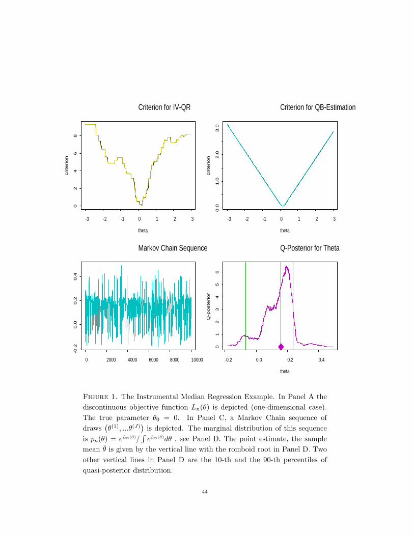
Criterion for IV-QR

theta

crite

rio

n

-3 -2 -1 0 1 2 3

02

46

8

Criterion for QB-Estimation

theta

crite

rio

n

-3 -2 -1 0 1 2 30

.01

.02

.03

.0

Markov Chain Sequence

0 2000 4000 6000 8000 10000

-0.2

0.0

0.2

0.4

Q-Posterior for Theta

theta

Q-p

oste

rio

r

-0.2 0.0 0.2 0.4

01

23

45

6

Figure 1. The Instrumental Median Regression Example. In Panel A thediscontinuous objective function Ln(θ) is depicted (one-dimensional case).The true parameter θ0 = 0. In Panel C, a Markov Chain sequence ofdraws

(θ(1), ...θ(J)

)is depicted. The marginal distribution of this sequence

is pn(θ) = eLn(θ)/∫

eLn(θ)dθ , see Panel D. The point estimate, the samplemean θ is given by the vertical line with the romboid root in Panel D. Twoother vertical lines in Panel D are the 10-th and the 90-th percentiles ofquasi-posterior distribution.

44

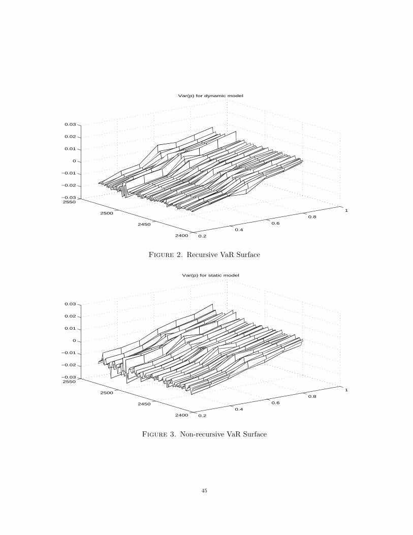
0.2

0.4

0.6

0.8

1

2400

2450

2500

2550−0.03

−0.02

−0.01

0

0.01

0.02

0.03

Var(p) for dynamic model

Figure 2. Recursive VaR Surface

0.2

0.4

0.6

0.8

1

2400

2450

2500

2550−0.03

−0.02

−0.01

0

0.01

0.02

0.03

Var(p) for static model

Figure 3. Non-recursive VaR Surface

45

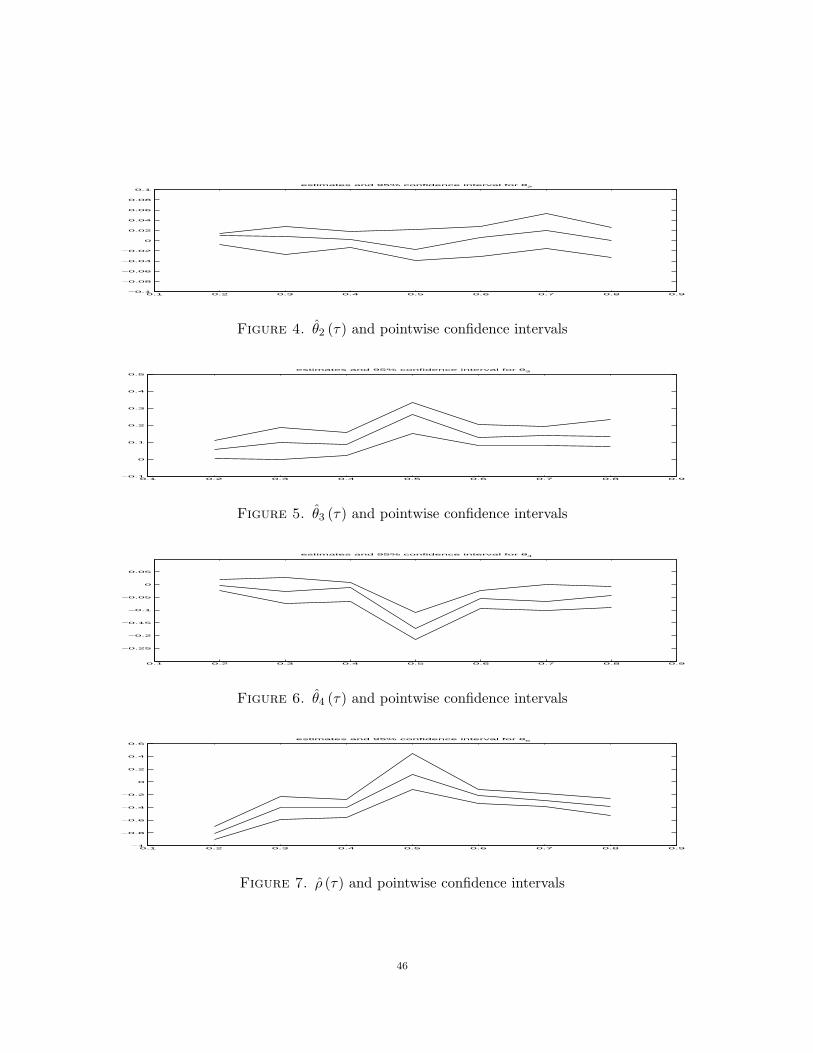
0.1 0.2 0.3 0.4 0.5 0.6 0.7 0.8 0.9−0.1

−0.08

−0.06

−0.04

−0.02

0

0.02

0.04

0.06

0.08

0.1

estimates and 95% confidence interval for θ2

Figure 4. θ2 (τ) and pointwise confidence intervals

0.1 0.2 0.3 0.4 0.5 0.6 0.7 0.8 0.9−0.1

0

0.1

0.2

0.3

0.4

0.5

estimates and 95% confidence interval for θ3

Figure 5. θ3 (τ) and pointwise confidence intervals

0.1 0.2 0.3 0.4 0.5 0.6 0.7 0.8 0.9

−0.25

−0.2

−0.15

−0.1

−0.05

0

0.05

estimates and 95% confidence interval for θ4

Figure 6. θ4 (τ) and pointwise confidence intervals

0.1 0.2 0.3 0.4 0.5 0.6 0.7 0.8 0.9−1

−0.8

−0.6

−0.4

−0.2

0

0.2

0.4

0.6

estimates and 95% confidence interval for θ5

Figure 7. ρ (τ) and pointwise confidence intervals

46