An Investigation of the Technical and Allocative Efficiency

of Broadacre Farmersa

Ben Hendersonb & Ross Kingwell

c

Contributed Paper to the 46th Annual Conference of the Australian Agricultural and Resource

Economics Society, 13-15 February, 2002, Rydges Lakeside Hotel, Canberra.

a This research has been supported by the Grains Research and Development Corporation,

the University of Western Australia and the Department of Agriculture. b MSc student, University of Western Australia

c Visiting senior lecturer, University of Western Australia and

Senior adviser, Western Australian Department of Agriculture

Abstract

The technical and allocative efficiency of broadacre farmers in a southern region of Western

Australia is investigated over a three-year period. Applying data envelopment analysis (DEA)

and stochastic frontier analysis (SFA) reveals there is some inefficiency in each year, which

decreases over time. The distributions of technical efficiency in each year are positively

skewed toward higher efficiency levels, indicating a majority of farms produce close to their

maximum technical efficiency. DEA and SFA produce similar efficiency rankings of farms

yet DEA rankings are more stable.

The relationships between farm-specific variables and the DEA and SFA efficiency scores are

investigated. There is evidence that farmers benefit from using at least a small amount of

tillage, rather than using ‘no-till’ practices. Education levels and farmer age are found to

positively influence technical efficiency.

Using a DEA profit efficiency model, the duality between the directional distance function

and the profit function allows the decomposition of economic efficiency into its technical and

allocative components. Greater gains in profitability are possible by improving allocative

rather than technical efficiency. Technically efficient farms are not necessarily allocatively

efficient. Also, Tobit regression results indicate that the variables associated with variation in

technical efficiency are different to those explaining the variation in allocative efficiency.

Key words: farm efficiency, data envelopment analysis, stochastic frontier analysis

1

Introduction

Farmers in Western Australia (WA) produce around a third of the Australian grain crop. They

have a relatively small domestic market, and therefore rely heavily on export markets

(ABARE/GRDC, 1999). Consequently, the economic sustainability of the WA broadacre

industry is highly dependent on maintaining and improving its international competitiveness

and profitability. These are contingent upon the prices paid for factors of production, prices

received for commodities produced and the productivity of farming operations.

The prices farmers receive for their commodities and pay for inputs are subject to variation,

mostly beyond the control of farm managers. As price-takers the most that individual farm

managers can do to increase their competitiveness, with regard to these prices, is to select the

most profitable combinations of inputs and outputs available to them. Farmers can also

improve their competitiveness in the long-term by increasing their level of productivity.

Improvements in productivity may arise through technological advances, improvements in

production efficiency and through exploiting scale economies. Technological improvements

such as the development of new herbicides, new crop varieties and advances in tractor and

machinery design, can improve the productivity of farms that adopt these new technologies.

On the other hand, improvements in production efficiency arise through better use of existing

technologies. Improving efficiency may be a more effective short-term solution to raising

productivity.

Broadacre farmers in Western Australia are known to have experienced higher levels of

productivity1 growth compared with producers from many other regions in the country, with

average per farm productivity growth of 3.5 per cent per annum over 21 years up until 1998-

1999 (Ha and Chapman, 2000). However, there are currently no studies that investigate

efficiency in WA broadacre agriculture.

To redress this neglect, this paper investigates the efficiency of a sample of WA broadacre

farms. This paper comprises 3 sections. The first section outlines some key concepts and

describes two methods of efficiency measurement. The second section presents an analysis of

farm-level efficiency of broadacre farms in a southern agricultural region of Western

Australia. A final section offers a set of conclusions and caveats on findings.

Section 1: Efficiency Concepts and Efficiency Measurement

In the literature on efficiency and performance measurement (e.g. Coelli et al 1998) two

related efficiency concepts are often discussed. The first is technical efficiency. In a farm-

setting this is the ability to produce maximal output from a given set of inputs, or where

output levels are fixed (e.g. by contract), to produce the output from a minimal set of inputs.

The second concept is known as price efficiency (Farrell 1957) or allocative efficiency (Färe

et al 1985). In a farm-setting this refers to the optimal selection of inputs, given their prices.

In other words, a combination of inputs is chosen to produce a set quantity of output at

minimum cost. However, allocative efficiency can also refer to the optimal combination of

outputs. This is particularly important in broadacre farming that is characterised by multiple

inputs (e.g. labour, machinery, fertilisers, fuel) and multiple outputs (e.g. wool, grain, sheep).

1 Productivity here refers to total factor productivity (TFP), which is inclusive of all inputs and outputs and is

constructed using a Tornqvist Index for aggregation.

2

There are two commonly used methods of measuring technical and allocative efficiency. The

following sub-sections describe briefly each method.

Data Envelopment Analysis

The origins of data envelopment analysis (DEA) lie with Farell (1957), yet it was Charnes et

al (1978) who first coined the term 'data envelopment analysis'. They suggested solving a set

of linear programs to identify the efficient production frontier and thereby estimate Farrell’s

radial measures of efficiency. Their approach overcame many of the computational

difficulties outlined by Farrell (1957), especially for cases involving multiple inputs and

outputs.

With DEA technical efficiency could be measured using either output-oriented or input-

oriented production function specifications. If constant returns to scale were assumed then

the output or input orientations would generate equivalent measures of technical efficiency.

DEA models could be modified to account for increasing or decreasing returns to scale

(Banker et al 1984). Also, when price and quantity data were available then DEA could also

measure allocative efficiency.

Färe et al. (1999) developed a set of linear programs to estimate a production function and

used directional distance functions (DDF) to estimate measures of technical inefficiency.

They also solved a second set of linear programs to estimate a profit function and its

corresponding measures of profit inefficiency. Measures of allocative efficiency could then be

obtained residually. They showed that the traditional input and output oriented DEA models

were special cases of the directional distance function (DDF). The DDF provided a tighter

'fit' around the data and thus identified lower levels of inefficiency than the traditional DEA

models.

Stochastic Frontier Analysis Not only did Farrell (1957) suggest using non-parametric approaches to efficiency

measurement but he also suggested using a parametric function, such as the Cobb-Douglas

function, to represent the efficient frontier. While a number of authors chose to estimate

production frontiers and Farrell measures of technical and allocative efficiency using non-

parametric approaches, another group employed parametric techniques. Aigner and Chu

(1968) used a Cobb-Douglas production function to estimate technical efficiency. Later, to

cope with statistical noise influencing frontier estimates Aigner et al (1977) and Meeusen and

van den Broeck (1977) independently proposed the now popular stochastic frontier analysis

(SFA) technique. They added a symmetric error term to their frontier models.

Following Afriat (1972) the parameters of their models were estimated using maximum

likelihood (ML) methods. Aigner et al (1977) assumed that the symmetrical error term, vi,

had a normal distribution and the one-sided error term, ui, had either a half normal or

exponential distribution2.

Stochastic frontier production functions can also be estimated using a method known as

corrected ordinary least squares, but as Coelli (1995) points out, the ML estimator is

asymptotically more efficient and should, therefore, be used in preference to the corrected

ordinary least squares estimator.

2 A more detailed outline of the stochastic frontier and its measure of efficiency can be found in chapter 4 of

Henderson (2002).

3

The Cobb-Douglas has been the most popular functional form in SFA applications, largely

because it is simple to apply3. However, its simplicity comes at the cost of some very

restrictive assumptions, including the assumption that all firms operate at the same scale and

that the marginal rate of input substitution (i.e. elasticities of substitution) is unity (Coelli

1995). Alternative forms such as the translog production function (Greene 1980) and the

Zellner-Revankar generalised production function (Kumbhakar et al 1991) have also been

suggested and applied. The first of these has a more flexible functional form than the Cobb-

Douglas, imposing no restrictions on returns to scale and input substitution, but it has the

unfortunate property of being susceptible to multicollinearity. Also, because many more

parameters are required than in an equivalent Cobb-Douglas model, larger data sets are

required to avoid problems associated with degrees of freedom.

Other developments include generalisations about the distributional assumptions of the one-

sided error term (ui). Stevenson (1980) proposed a truncated-normal distribution for ui,

assumed to be normally distributed with a non-zero (constant) mean truncated at zero from

above. This more general distribution accounted for situations in which the majority of firms

were not in the neighbourhood of full technical efficiency. Another generalisation follows the

approach outlined by Reifshneider and Stevenson (1991) and Kumbhakar et al (1991), in

which ui is estimated as an explicit function of firm-specific factors. Previously, firm specific

factors were regressed in a second stage on technical efficiency scores estimated by the

stochastic frontier in the first stage. The problem with this approach is that the uis are assumed

to be independently and identically distributed in the first stage, but they are assumed to be a

function of a number of firm-specific variables, rather than being independently and

identically distributed in the second stage (Coelli, 1995).

Besides measures of technical efficiency, measures of cost efficiency can also be obtained

using SFA if a cost function is derived. Drawing on the duality between the cost function and

the production function, cost inefficiency estimates can be decomposed into their technical

and allocative components. For more on this see Coelli et al (1998).

Strengths and Weaknesses of DEA and SFA

The arguments for and against the application of either approach revolve around their

respective strengths and weaknesses. SFA, as a parametric approach, requires the

specification of a functional form for the production frontier, which implies that the actual

shape of the frontier is known. Also, parametric measures of efficiency make assumptions

about the distribution of efficiency. This is the main shortcoming of the SFA method to

estimate efficiency. However, these assumptions permit statistical hypothesis testing of the

most likely shape of the frontier and of the distribution of inefficiency. Hypothesis tests for

the significance of inefficiency in the model are also possible.

The DEA approach, on the other hand, is non-parametric and employs linear programming

techniques to construct a frontier. The DEA frontier is made up of actual observations and

because it does not rely on the specification of a functional form for the frontier, it is free

from assumptions about its shape. DEA also makes no assumptions about the distribution of

efficiency. In instances where multiple outputs need to be specified, DEA would be the

preferred method, because it can accommodate them more easily. Despite these advantages of

the DEA approach, its deterministic nature raises questions about its usefulness in situations

where statistical noise is likely to affect results.

3 A logarithmic transformation produces a model that is linear in the logarithms of the inputs (Coelli 1995)

4

The stochastic frontier approach, as its name suggests, can cope with statistical noise, which

may be present in the data as a result of measurement errors, missing variables, and variation

in weather conditions. DEA on the other hand is deterministic, attributing all variation from

the frontier to inefficiency, which is a questionable assumption if there is significant statistical

noise in the data (Coelli 1995)4. Coelli et al (1998) argue that in agricultural industries with

controlled production environments (e.g. intensive industries such as piggeries) and where the

quality of inputs and outputs does not vary from firm to firm, DEA may be the preferred

method. While record-keeping might be accurate, and while many outputs and factors of

production are often homogenous in broadacre agriculture, the uncontrollable impact of

weather and resource quality on production is likely to contribute to the statistical noise in the

data. However, where weather effects and their impact on production can be measured, their

impact on shaping the frontier and efficiency scores may be accounted for.

Another criticism often levelled at the DEA approach is that, unlike SFA, there is a lack of

formal tests available to assess the validity of the functional form created by optimisation of

the DEA problem. However, a number of such formal tests for non-parametric techniques

such as DEA have and are still being developed. Some of these tests are outlined in Banker

(1989) and Banker (1996).

The DEA approach is superior to SFA with regard to the amount of useful information it

provides. For example, the DEA approach identifies, for every inefficient firm, technically

efficient firms which have a similar production mix (i.e. their efficient peers) which could be

useful for farm management because it provides a practical example for inefficient farms of

how much more productive they might be.

Finally, a problem with all approaches to measuring frontier efficiency, noted by

Farrell (1957), is that the technical efficiency of a firm must always, to some extent, reflect

the quality of its inputs. Many practitioners make attempts to homogenise input and output

qualities with varying approaches and success. In the dairy literature milk is often expressed

in fat and protein equivalents in an attempt to homogenise output. Coelli et al (1998) list a

number of weaknesses that apply to both DEA and SFA, including the fact that these

techniques cannot easily account for risk in decision-making. Further, they comment that it is

not possible to compare mean efficiency scores from a study that draws on one sample with a

study that uses another sample, although comparing the spread or distribution of efficiency

between samples is both useful and permissible.

DEA and SFA Studies of Broadacre Agriculture in Australia

Henderson (2002) presents a detailed review of DEA and SFA studies of various agricultural

industries. He identifies a small set of studies dealing with broadacre agriculture in Australia.

Chapman et al (1999) examine wool producers and use expenditure data rather than

quantities, and consequently refer to their results as productivity indexes rather than technical

efficiency scores5. They use spatial information to make comparisons of the productivity

measures with a map of seasonal rainfall. They found that areas with lower productivity

scores tended to have poorer seasonal conditions. To gauge the impact of resource quality on

4 Some work has been done by (Banker 1989) in developing a stochastic DEA frontier.

5 Thomas and Tauer (1994) demonstrate graphically, mathematically and empirically that linear aggregation by

value downwardly biases technical efficiency scores, because the technical efficiency measure post-aggregation

is a compound of technical and allocative efficiencies.

5

productivity, the correlation between land values and productivity was examined and the two

were found to be positively correlated.

Fraser and Hone (2001) like Chapman et al (1999) focused on wool production. The authors

solved two different DEA models using a panel of Victorian wool producers from 1990-91 to

1997-98. The first model was an output-orientated DEA model used to calculate measures of

technical efficiency in each year. The second involved using DEA to calculate Malmquist

estimates of total factor productivity. In the first part of the analysis the stability of technical

efficiency measures was investigated by observing the movement of efficient farms from one

season to the next. The results indicated that there was little stability, as only one farm was

found to be fully efficient over the entire study period. Spearman coefficients of rank

correlation were the measures of the stability of efficiency ranks between seasons. Significant

correlation between ranks was generally found. Despite this the authors still argued that

variation in technical efficiency scores was high enough to suggest that farm-specific factors

other than managerial ability may have been captured and consequently, that the measures

should be treated with caution. The relationship between farms’ enterprise mixtures and

technical efficiency was also investigated; farms with a mixture of enterprises were found to

be slightly more efficient than those that focused primarily on wool production.

The Malmquist total factor productivity measures revealed that the productivity of Victorian

wool producers declined by an average of 2.5 per cent over the study period, and that this was

caused by contraction of the production frontier rather than a decline in the technical

efficiency of producers. Finally, the authors warned that single period estimates of technical

efficiency should be viewed cautiously, because management decisions may be consistent

with accounting for production risks, such as disease out-breaks, but may result in lower

short-run levels of technical efficiency.

Fraser and Cordina (1999) used cross sectional data on Victorian dairy farms over two

consecutive lactation seasons to calculate both variable returns to scale and constant returns to

scale frontiers. The motivation for their paper was to assess whether gains in efficiency could

be made to offset future water supply restrictions. The correlation between farm size and

technical efficiency was examined too, and was found to be insignificant. Fraser and Cordina

(1999) were also interested in the temporal stability of the frontier, suggesting that significant

instability would cast doubt on the reliability of the DEA applications to agriculture. Three

different hypothesis tests were used to compare the technical efficiency scores from both

seasons. These tests were, the Wilcoxon signed-rank test for matched pairs (non-parametric),

and two parametric t-tests, one assuming unequal variance and one assuming equal variance.

The authors found that the technical efficiency scores between the seasons were not

significantly different. An interesting ‘rule of thumb’ they suggested was that there should

always at least three times as many data observations as variables. They considered that, if the

ratio of variables to observations is greater than 1:3, then the problem of self-referencing

would upwardly bias technical efficiency scores and reduce the discriminating power of the

analysis. This is in contrast to Fernandez-Cornejo (1994), who insisted that the ratio of

variables to observations be no higher than 1:5.

Battese and Corra (1977) was one of the first applications of SFA to farm-level data. Iit was

also the first study of its kind to be applied to Australian farm-level data. The data came from

a sample of sheep producers in the pastoral zone of eastern Australia. The maximum

likelihood values of the variable coefficients were presented and the significance of both the

one-sided and symmetric error terms were found to be significant, i.e. both the technical

6

inefficiency effects and the stochastic effects were significant. The only other SFA application

to Australian farm-level data is by Battese and Coelli (1988) who used a three-year panel of

dairy farms spanning production regions in Victoria and New South Wales. In this study a

generalisation of the technique suggested by Jondrow et al. (1982) for determining firm-level

technical efficiency was proposed, which permitted estimation using panel data and assumed

a more general distribution for the one-sided error term suggested by Stevenson (1980).

Technical efficiency was found to be significant and significantly different between each

State.

Section 2: An analysis of broadacre farm efficiency in a region of

Western Australia

The technical and allocative efficiency of a sample of farms drawn from the southeast and

south coast agricultural regions of Western Australia (see figure 1) was measured using DEA

and SFA. The nature of the DEA and SFA models is described in the following sub-sections.

The sample comprised 93 farms with detailed price and quantity data for each year 1997 to

1999. The data were supplied by farm management consultants operating in the region.

DEA Model

The DEA model is based on the simultaneous expansion of outputs and contraction of inputs

and is used to derive a measure of technical inefficiency for each farm in the sample.

Mathematically, the model is described by equation (1).

max )g,gy;(x,DTIE yxT

(1)

subject to:

'in'inin

N

1n

n yyy

i = 1,…, I

'kn'knkn

N

1n

n xxx

k = 1,…, K

1N

1n

n

λn ≥ 0, n = 1,…, N .

For farm n', the K inputs and I outputs are represented by the vectors xkn' for k =1,…, K inputs

and yin' for the outputs i = 1,…, I, respectively. The frontier envelops the data points such that

all observed points lie below or to the right of the frontier.

The λs are weights used to construct the efficient frontier. They also determine the point on

the frontier where inefficient farms would be producing if they were efficient. Thus, the

hypothetical point of maximum efficiency for an inefficient farm is determined by the

weighted average of the bundle of inputs and outputs for efficient farms on the frontier.

Looking at the constraints in equation (1):

The first one states that farm n’s i-th output will be scaled up by β to an output level no

greater than that created by the weighted linear combination of farm n’s efficient peers. The

7

8

second constraint states that farm n’s k-th input is also scaled down y β (note the negative

sign on 'knx ) to an input level no smaller than that created by the weighted linear

combination of farm n’s efficient peers. Maximising β subject to both of these constraints

brings farm n to a hypothetical point on the surface of the production frontier. The Σ = 1

constraint relaxes the assumption that all farms are producing at an optimal scale, i.e. constant

returns to scale (CRS) is not imposed. The λn ≥ 0 constraint is a non-negativity constraint,

and ensures that none of the hypothetical points making up the frontier are in negative

quadrants, i.e. both the farm's inputs and outputs need to be positive.

β will satisfy 0 ≤ β < ∞ as a measure of technical inefficiency, with zero representing a fully

efficient farm. To obtain a β value for each farm, equation 1, a linear programming problem,

must be solved N times for each sample farm.

SFA Model The SFA model is represented mathematically as equation (2).

ln(yi) = f (xi; β) + vi – ui, i = 1,2, … , N (2)

where:

ln(yi) is the log of the observed level of production of the i-th firm;

xi is a (1 x k) vector of functions of input quantities used by the i-th firm;

β is a (k x 1) vector of unknown parameters to be estimated;

vis are random variables accounting for measurement error and other random factors such as

the effects of weather on the value of yi, as well as the combined effects of unspecified input

variables in the production function. They are assumed to be independent and identically

distributed normal random variables having zero mean and constant variance N (0, σV2) and

are independent of,

uis which are non-negative random variables that account for the technical inefficiency in

production, and are often assumed to be independent and identically distributed with

truncations at zero of the N(μ, σu2) distribution.

The computer program, Frontier Version 4.1c6, generates the ML estimates for the model

parameters. The conditional expectation of ui, given the value of vi – ui, is used to predict the

farm level technical efficiency scores. For more detail see Coelli et al (1998).

Data

Data from over 100 farmers for up to 5 consecutive years initially were gathered. Farms in

this region are mixed, with most farm income coming from cropping enterprises. The data

were detailed records of physical and financial items. Using ancillary data, indexing

techniques and after clarifying data for some individual farms, each farm's data in each year

were re-expressed as a series of input and output indexes. Missing data precluded the use of

all of the observations in each year, leaving a reduced yet complete sample of 93 farms over 3

consecutive years.

6 Developed by Tim Coelli, Centre for Efficiency and Productivity Analysis, UNE.

9

The DEA model comprised the following variables:

Outputs Inputs

Crops (O1) Capital (I1)

Livestock (O2) Labour (I2)

Materials (I3)

Services (I4)

Summary statistics for these variables are listed in table 1. Over the period the average value

of cropping enterprises rose, while the average value of livestock enterprises declined. The

reduction in the value of the livestock enterprises was due mainly to a switch of land

resources into more cropping and a reduction in the size of the sheep flock. ABARE (1999)

reported these same enterprise trends for the central and southern broadacre farming regions

of Western Australia. There was a large variation in the size of farms in the sample, leading

to relatively large coefficients of variation in most input and output categories.

The SFA frontier was specified using the same variables, except that due to the frontier-fitting

software (FRONTIER 4.1 (Coelli 1996)) not being able to cope with multiple outputs, crops

and livestock items were aggregated to create a single output category.

Table 1: Summary statistics for the value of inputs and outputs in each year.

Year/

Variable

Mean Min Value Max Value Coefficient of

variation (%)7

1997

Crop ($) 301,858 9,463 963,654 67.2

Livestock ($) 125,437 22,274 527,659 57.1

Capital ($) 207,775 61,904 600,837 47.9

Labour ($) 56,332 20,012 137,014 43.8

Materials ($) 156,191 14,843 989,840 80.5

Services ($) 105,339 28,606 309,809 55.5

1998

Crop ($) 308,850 1,667 882,447 63.7

Livestock ($) 109,733 22,490 468,659 58.1

Capital ($) 217,903 65,012 673,565 43.8

Labour ($) 57,988 22,008 168,715 44.7

Materials ($) 145,701 21,852 380,756 56.3

Services ($) 99,375 26,579 262,695 45.5

1999

Crop ($) 347,368 4,026 992,234 64.2

Livestock ($) 104,090 19,287 329,826 56.8

Capital ($) 184,943 61,139 515,885 47.6

Labour ($) 59,454 20,942 141,623 41.6

Materials ($) 152,909 25,584 451,239 63.7

Services ($) 107,077 35,897 285,308 46.6

To derive the input and output categories required aggregation. For example, crop output was

based on the aggregation of data involving several crop types including wheat, barley, oats,

7 Coefficient of variation = (standard deviation / mean) * 100

10

lupins, canola and pulses. Aggregation involved the Fisher Index, adjusted by the EKS

method (Elteto and Koves 1964, Szulc 1964), to derive multilateral transitive Fisher indices.

See appendix one and Henderson (2002) for more detail on the aggregation process and data

sources.

Besides the production and price data, information was also collected on farm-specific

variables that might assist in explaining the variations in farm-level efficiency. These

explanatory variables were:

Age (Z1)

Age2 (Z2)

Rainfall (Z3)

Minimum Tillage (Z4)

Direct Drilling (Z5)

Education (Z6) and

Land (Z7)

Their sample characteristics are given in table 2.

Table 2: Summary of farm-specific characteristics.

Farm-specific characteristic Unit 1997 1998 1999

Average age Years - - 48

Average annual rainfall mm 436 488 440

Average crop yield kg/ha 1890 1900 2207

No. using minimum tillage no. 58 58 58

No. using direct drilling no. 26 26 26

No. using multiple tillage no. 9 9 9

No. with year 10 education no. 52 52 52

No. with > year 10 education no 41 41 41

Average farm size ha 2175 2133 2174

Age (Z1) is measured as the age of the farm operator in years and can also be viewed as a

proxy for farming experience. The relationship of this variable to efficiency, for reasons given

in chapter 3, could be negative or positive.

Age2 (Z2) is simply the square of Z1. The inclusion of this variable allows the simple testing

of the ‘life-cycle’ hypothesis. According to this hypothesis, the efficiency of the farmer

increases at first with age and then decreases once the farmer is beyond middle age. If Z2 is

found to be significant then the relationship between farmer age and efficiency can be

considered quadratic, increasing at first with age and then decreasing with age. The quadratic

relationship specified by this variable makes a few restrictive assumptions including that the

rate of increase and decrease of efficiency with farmer age is symmetrical. However, this

assumption may not be unrealistic as Tauer (1984) and Tauer (1995) report such symmetry in

their findings.

Rainfall (Z3) represents the rainfall in millimetres in the calendar year, and is expected to have

a positive effect on technical efficiency. This is because rainfall is directly and positively

related to yield; in fact it is the largest natural driver of yields in broadacre dryland farming

Western Australia (DAWA 1991, AWA 2000). Rainfall throughout the WA wheatbelt is a

11

highly variable and scarce resource, so it is often the main factor influencing farm

performance. Despite rainfall being a very important input in rainfed production processes, it

does not typically enter the production function because it is a factor not under the control of

the farm manager.

Given that rainfall is inextricably linked to yield, it is important to not only measure the

impact of this variable on efficiency, but also to account for its impact on efficiency. Coelli et

al (1998) suggest some approaches for accounting for environmental variables such as

rainfall.

The methods of crop establishment used by farm operators are grouped into three broad

categories; minimum tillage, direct drilling, and multiple tillage techniques. Two binary

dummy variables account for the effect that each of these techniques has on efficiency. The

first of these, minimum tillage (Z4), assigns a value of 1 to farms whose crops are established

with minimum tillage and a value of zero for all others. The second of the crop establishment

dummy variables, direct drilling (Z5), assigns a value of 1 to farms applying direct drilling to

establish crops and a value of zero for all others.

Conventional or multiple tillage involves ploughing8 or turning over the soil several times,

and is the traditional method of seedbed preparation for WA broadacre farmers. Some of the

benefits of this practice include killing weeds, aerating and loosening the soil to aid root

growth, mineralizing soil nitrogen and other nutrients to increase their availability to newly

established crops, and for controlling root diseases. Rhizoctonia, a root pathogen that is a

particular problem on the Esperance sandplain, is one of many diseases reduced by

cultivation.

Until the 1970s conventional cultivation was seen as essential for successful cropping.

Despite its benefits, evidence emerged suggesting that these cultivation practices had some

undesirable side effects, which could, in the long-term, reduce soil productivity and therefore

technical efficiency. These include an increased risk of wind erosion, loss of organic matter,

delayed time of seeding, increased weed germination and poorer pasture re-establishment

after crop production. Acknowledgement of these negative attributes and the development of

better and more affordable herbicides from the 1970s onwards led to the development of

alternative crop establishment practices reliant on reduced tillage. Many different crop

establishment techniques now come under the umbrella of reduced or minimum tillage. In this

study minimum tillage refers to tillage of the entire topsoil using only one or two cultivations

prior to sowing, while direct drilling typically involves sowing in a single pass in previously

uncultivated soil (ABARE 2000). This technique can improve soil properties and preserve its

long-term productivity, by retaining soil organic matter and reducing soil erosion. This can

help to increase microbiological activity in the soil and increase fertility through the

modification of the soils' physical, chemical and biological components. Bligh and Findlater

(1996) outline other benefits associated with no-till farming.

While all of the soils in the study region can support no-till operations, sandy soils are the

most typical in the WA wheatbelt and yet these soils are the least responsive to the benefits of

no-till practices. This is largely due to the fact that these soils have little structure and often

8 Disc ploughs, tined scarifiers and chisel ploughs are the primary cultivation equipment.

12

form surface 'hard pans', after rainfall and farm traffic, that restrict the early development of

crop roots and hence crop yields9. Tillage removes these surface 'hard pans'.

The choice of ‘no-till’ versus ’min-till’ involves considering a range trade-offs. Farms on the

south coast of WA, which make up a significant proportion of sample farms (see figure 1),

typically have fine sands that are particularly susceptible to erosion and don’t form surface

crusts. In these instances, 'no-till' methods of crop establishment may improve the productive

capacity of the soil and subsequently, the productive performance of the farm.

Education (Z6) of the farm operator is measured by a simple binary dummy variable; farmers

educated at the level of year 12 and above are assigned a value of one and farmers educated

below this level are assigned a value of 0. This variable captures the main source of variation

in education between farmers. Education is expected to be positively related to efficiency,

because it should increase farmers' capacity to process the information necessary to apply

‘best practices’.

Land (Z8) represents the number of hectares operated on the farm. Farm size is expected to be

positively related to efficiency.

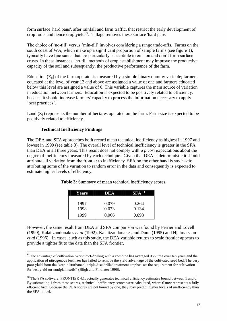
Technical Inefficiency Findings

The DEA and SFA approaches both record mean technical inefficiency as highest in 1997 and

lowest in 1999 (see table 3). The overall level of technical inefficiency is greater in the SFA

than DEA in all three years. This result does not comply with a priori expectations about the

degree of inefficiency measured by each technique. Given that DEA is deterministic it should

attribute all variation from the frontier to inefficiency. SFA on the other hand is stochastic

attributing some of the variation to random error in the data and consequently is expected to

estimate higher levels of efficiency.

Table 3: Summary of mean technical inefficiency scores.

Years DEA SFA 10

1997 0.079 0.264

1998 0.073 0.134

1999 0.066 0.093

However, the same result from DEA and SFA comparison was found by Ferrier and Lovell

(1990), Kalaitzandonakes et al (1992), Kalaitzandonakes and Dunn (1995) and Hjalmarsson

et al (1996). In cases, such as this study, the DEA variable returns to scale frontier appears to

provide a tighter fit to the data than the SFA frontier.

9 “the advantage of cultivation over direct-drilling with a combine has averaged 0.27 t/ha over ten years and the

application of nitrogenous fertilizer has failed to remove the yield advantage of the cultivated seed bed. The very

poor yield from the ‘zero-disturbance’, triple disc drilled treatment emphasises the requirement for cultivation

for best yield on sandplain soils” (Bligh and Findlater 1996). 10

The SFA software, FRONTIER 4.1, actually generates technical efficiency estimates bound between 1 and 0.

By subtracting 1 from these scores, technical inefficiency scores were calculated, where 0 now represents a fully

efficient firm. Because the DEA scores are not bound by one, they may predict higher levels of inefficiency than

the SFA model.

13

Table 4 outlines the distributions of the various technical inefficiency series. The SFA

technical efficiency distributions, like the DEA technical inefficiency distributions, are highly

skewed with a greater proportion of farms in the samples being close to the frontier. An

obvious difference is that, according to the SFA approach, none of the sample farms were

fully efficient, whereas 33 per cent were fully efficient when DEA was used. This is solely

due to the differences in the way the respective frontiers are constructed. In DEA actual

observations are used to construct the frontier, therefore a number of farms will inevitably be

estimated as being fully efficient. Temporally, the distributions follow a similar pattern; both

DEA and SFA distributions become more skewed as efficiency increases across time. This

decline in technical inefficiency implies that farms are moving closer to the frontier over time.

One implication is that over the sample period farms are gradually adopting more productive

techniques and improving their technical management of enterprises.

Table 4: Technical inefficiency distributionsa.

Inefficiency

Range

1997

1998 1999 1997

1998 1999

SFA DEA

0.0 0 0 0 33 37 36

0.0 – 0.1 23 48 73 23 26 34

0.1 – 0.2 12 26 11 29 21 14

0.2 – 0.3 16 13 4 6 8 6

0.3 – 0.4 18 4 2 2 1 3

0.4 – 0.5 17 2 3

0.5 – 0.6 6

0.6 – 0.7 a Figures in each cell refer to the number of farms recording a technical inefficiency in that range.

Sources of Technical Inefficiency

Using DEA it is possible to examine possible sources of technical inefficiency; that is, which

inputs are being overused and what outputs under-produced. Table 5 demonstrates where

gains in efficiency could have been made for the average farm in 1997, 1998 and 1999,

according to the DEA analysis.

On average farmers are inefficient in the use of all inputs and outputs in all years. In 1997

output levels could be increased by an average of 6.4 per cent and input levels could be

reduced by an average of 16.4 per cent through gains in technical efficiency. In 1998 similar

increases in output levels are suggested as achievable, while the level of input contraction is

slightly less at 15.1 per cent. In 1999 the gains and reductions in outputs and inputs are

slightly more modest at 6.0 per cent and 10.7 per cent respectively. The input used most

inefficiently in each year is capital, while the gains in efficiency that can be made by

expanding outputs are split evenly between the crop and livestock enterprises.

14

Table 5: Identifying potential gains in efficiency.

Crop Livestock Capital Labour Materials Services

1997

Original levels 2.250 0.799 0.961 0.773 1.035 1.425

Optimal levels 2.400 0.857 0.760 0.660 0.939 1.148

Potential gains (%) 6.2 6.7 -20.8 -14.6 -9.2 -19.4

1998

Original levels 1.890 0.563 0.875 0.643 1.097 1.415

Optimal levels 2.023 0.602 0.658 0.570 0.957 1.237

Potential gains (%) 6.5 6.4 24.8 -11.2 -12.7 -12.6

1999

Original levels 2.547 0.438 0.700 0.720 1.267 0.862

Optimal levels 2.697 0.478 0.628 0.656 1.141 0.741

Potential gains (%) 6.5 6.4 -16.6 -10.9 -12.8 -12.5

Summary: Total gains

in outputs

Total reductions

in inputs

1997 6.4% 16.4%

1998 6.5% 15.1%

1999 6.0% 10.7%

Possible sources of technical inefficiency can also be examined using SFA and its findings are

that output could have been expanded by 26.4, 13.4 and 9.3 per cent in 1997, 1998 and 1999

respectively. Because SFA produces output-oriented measures of efficiency, these potential

gains in output are calculated while holding input levels fixed. Therefore, it is not surprising

that SFA produces more generous estimates of potential output than the directional distance

function DEA model. SFA also produces more optimistic estimates of potential gains in

output because it identified higher mean levels of inefficiency (Table 3).

Comparing DEA and SFA Technical Efficiency Rankings

Are DEA and SFA technical efficiency rankings consistent?

Spearman coefficients of rank correlation were calculated to test whether or not the two

approaches produced similar efficiency rankings in each year. The magnitude of efficiency

identified by each approach is not as important as their relative efficiency rankings because

the magnitude of inefficiency identified is fairly arbitrary, depending largely on the direction

used and assumptions about the shape and nature of the frontier (Chambers 2000). If rankings

are similar, then the identification of top and bottom performers is thus not sensitive to the

choice of methodology.

The following hypothesis is tested:

H0: rs = 0, i.e. there is no significant correlation between DEA and SFA efficiency rankings.

H1: rs ≠ 0, i.e. there is significant positive correlation between DEA and SFA efficiency

rankings.

Results in table 6 show significant and positive rank agreement between the technical

efficiency series generated by the two methods in all three years. This suggests that farm

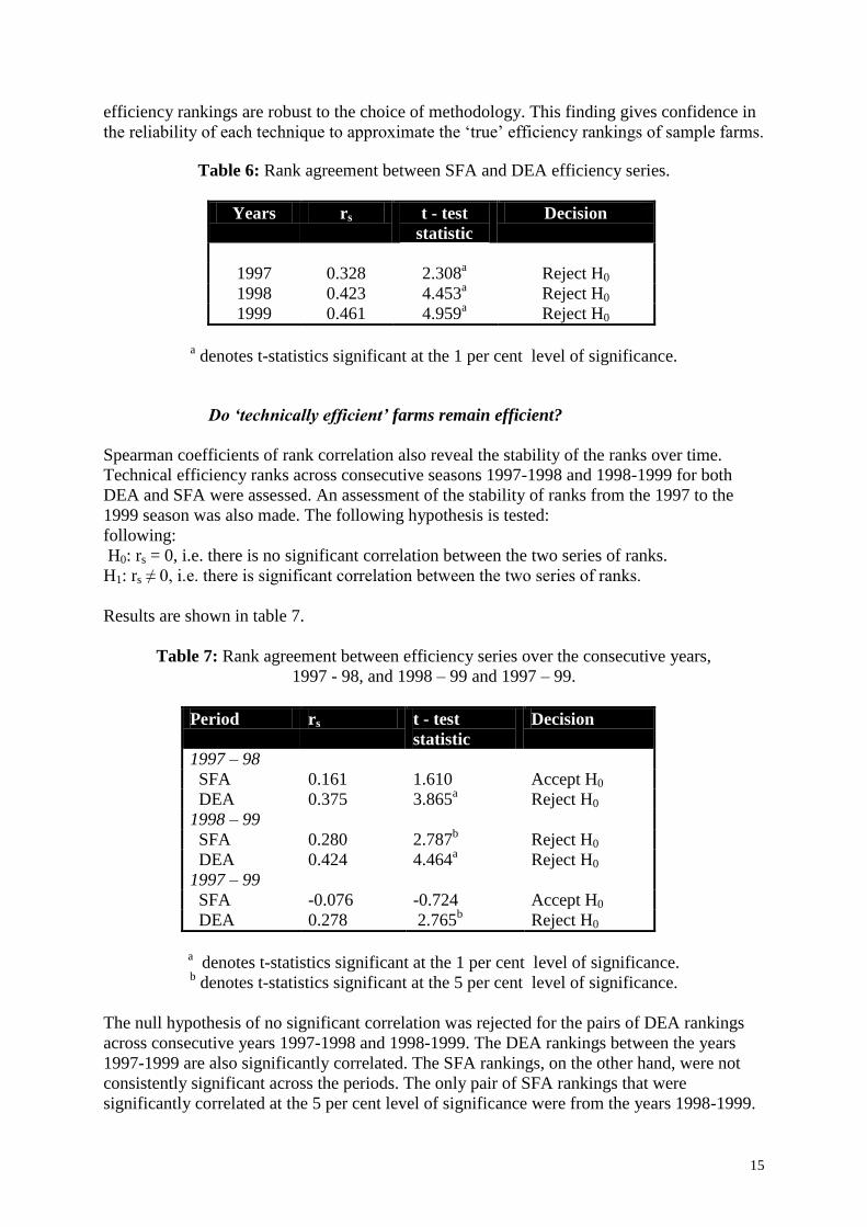
15

efficiency rankings are robust to the choice of methodology. This finding gives confidence in

the reliability of each technique to approximate the ‘true’ efficiency rankings of sample farms.

Table 6: Rank agreement between SFA and DEA efficiency series.

Years rs t - test

statistic

Decision

1997 0.328 2.308a Reject H0

1998 0.423 4.453a Reject H0

1999 0.461 4.959a Reject H0

a denotes t-statistics significant at the 1 per cent level of significance.

Do ‘technically efficient’ farms remain efficient?

Spearman coefficients of rank correlation also reveal the stability of the ranks over time.

Technical efficiency ranks across consecutive seasons 1997-1998 and 1998-1999 for both

DEA and SFA were assessed. An assessment of the stability of ranks from the 1997 to the

1999 season was also made. The following hypothesis is tested:

following:

H0: rs = 0, i.e. there is no significant correlation between the two series of ranks.

H1: rs ≠ 0, i.e. there is significant correlation between the two series of ranks.

Results are shown in table 7.

Table 7: Rank agreement between efficiency series over the consecutive years,

1997 - 98, and 1998 – 99 and 1997 – 99.

Period rs t - test

statistic

Decision

1997 – 98

SFA 0.161 1.610 Accept H0

DEA 0.375 3.865a Reject H0

1998 – 99

SFA 0.280 2.787b Reject H0

DEA 0.424 4.464a Reject H0

1997 – 99

SFA -0.076 -0.724 Accept H0

DEA 0.278 2.765b Reject H0

a denotes t-statistics significant at the 1 per cent level of significance.

b denotes t-statistics significant at the 5 per cent level of significance.

The null hypothesis of no significant correlation was rejected for the pairs of DEA rankings

across consecutive years 1997-1998 and 1998-1999. The DEA rankings between the years

1997-1999 are also significantly correlated. The SFA rankings, on the other hand, were not

consistently significant across the periods. The only pair of SFA rankings that were

significantly correlated at the 5 per cent level of significance were from the years 1998-1999.

16

Henderson (2002) also conducted a conditional probability analysis to examine the stability of

technical efficiency rankings through time. The findings supported results in table 7 with the

conclusion that DEA efficiency rankings are more stable over time than equivalent SFA

rankings.

The movement of farms in and out of the DEA ‘efficient set’ (i.e. those efficient farms that

are part of the frontier) is listed in table 8. This provides evidence specifically about the

persistence of technical efficiency and also about the stability of the DEA envelope.

Table 8: The movement of farms in and out of the ‘efficient set’.

Year No. of

efficient

farms

No. remaining

efficient after one

season

No. remaining

efficient after

two seasons

1997 33 19 10

1998 37 21 na

1999 36 na na na not applicable

A majority of farms remain in the ‘efficient set’ from one year to the next: 18 out of 31 farms

(58 per cent) remained efficient from 1997 to 1998 and 22 out 36 (61 per cent) remained

efficient from 1998 to 1999. The movement of farms out of the ‘efficient set’ over the three

years was much higher with only 10 out 33 farms (30 per cent) remaining efficient from 1997

to 1999.

What influences technical efficiency?

DEA

The impact of farm-specific variables, described previously, on measures of technical

inefficiency was investigated using regression analysis. A Tobit regression model was used to

model DEA technical inefficiency scores, with farm-specific variables included directly in the

production function to model technical inefficiency in a single stage parametric approach. The

Tobit regression results are shown in table 9.

Three of the explanatory variables tested explain a significant amount of the variation in

technical inefficiency for 1997. These include rainfall and both of the crop establishment

dummy variables. However, the first crop establishment dummy variable (Z4) is only

significant at the 10 per cent level. The second crop establishment dummy variable (Z5) has a

higher level of significance at 5 per cent. Z5 has a positive sign, and a higher coefficient value

and level of significance than Z4. This indicates that farmers using no-till methods or direct

drilling when establishing their crops are more technically inefficient than those farmers

employing either minimum or multiple tillage practices. Given that most of the sample farms

use minimum tillage practices (62 percent), this positive sign signifies that farms practising

no-till farming (28 percent of sample farms) are not as efficient as those using minimum

tillage. This could be caused by a positive yield response to any or all of the beneficial effects

of tillage, which include weed control, aerating and loosening soils to aid root growth,

mineralizing soil nitrogen and other nutrients to increase their availability to newly

established crops, and for controlling root diseases such as rhizoctonia. This result indicates

17

that, in the study region, the benefits listed above outweigh those, such as the minimisation of

soil erosion and lower labour and machinery requirements, that are associated with no-till

farming.

Finally, the significant and positive relationship between rainfall and efficiency supports a

priori expectations. This is due to the direct and positive impact of rainfall on crop and

pasture yields.

Table 9: Tobit regression DEA results.

IE/Variable Parameters Coefficient Standard

error

t-ratio

1997

Intercept δ0 3.714 3.579 1.037

Age (Z1) δ1 -0.117 0.151 -0.770

Age2 (Z2) δ2 1.33E-03 1.56E-03 0.854

Rainfall (Z3) δ3 -2.53E-03 1.19E-03 -2.128b

Min till D (Z4) δ4 0.717 0.375 1.909c

Direct drill D (Z5) δ5 1.099 0.424 2.587b

Education (Z6) δ6 -0.209 0.249 -0.837

Land (Z8) δ8 -1.72E-04 1.10E-04 -1.562

Log likelihood 19.278

1998

Intercept δ0 5.998 3.641 1.648

Age (Z1) δ1 -0.203 0.156 -1.299

Age2 (Z2) δ2 1.83E-03 1.60E-03 1.145

Rainfall (Z3) δ3 -2.05E-03 1.11E-03 -1.848c

Min till D (Z4) δ4 0.603 0.378 1.596

Direct drill D (Z5) δ5 0.966 0.413 2.340b

Education (Z6) δ6 -0.251 0.250 -1.003

Land (Z8) δ8 1.18E-04 1.33E-04 0.891

Log likelihood 14.735

1999

Intercept δ0 6.062 3.654 1.659

Age (Z1) δ1 -0.220 0.152 -1.452

Age2 (Z2) δ2 2.32E-03 1.56E-03 1.484

Rainfall (Z3) δ3 -2.98E-03 1.31E-03 -2.269b

Min till D (Z4) δ4 0.325 0.379 0.857

Direct drill D (Z5) δ5 0.463 0.400 1.154

Education (Z6) δ6 7.41E-02 0.2471 0.300

Land (Z8) δ8 1.13E-04 1.19E-04 0.953

Log likelihood 13.576

b and

c denote t-statistics significant at the 5 per cent and 10 per cent levels of significance.

The 1998 Tobit regression results paint a very similar picture. Rainfall and direct drill

coefficients, δ3 and δ5, are of a similar magnitude and level of significance as in 1997. The

18

minimum tillage variable, however, is not found to be significant, even at the 10 per cent

level. Farms practising no-till are found to be more technically inefficient than those using

either minimum tillage or multiple tillage practices. Again this indicates the positive benefits

from the small amount of tillage involved with minimum tillage, outweigh those associated

with no-till farming. However, this time the positive effect of rainfall on efficiency is only

significant at the 10 per cent level of significance.

In 1999 rainfall explains most of the variation in technical inefficiency and its effect on

efficiency is positive and significant at the 5 per cent level of significance. In this year neither

of the crop establishment dummy variables explain a significant amount of the variation in

efficiency.

SFA

The results from the SFA technical efficiency effects model tell a different story to that of the

Tobit analysis on the DEA scores. In 1997 land (Z7) was the only explanatory variable with a

significant effect on efficiency (see table 10). The relationship between land and efficiency in

this case was positive and highly significant at the 1 per cent level. This supports a priori

expectations that larger farms would perform better.

In 1998 the land variable is no longer significantly or positively related to efficiency. Age (Z1)

and age2 (Z2) are now significantly and positively related to efficiency at the 10 per cent level

of significance. The first of these results indicates that older farmers, on average, perform

better than young farmers as technical managers, possibly because due to their experience.

The second finding provides some support for the ‘life cycle’ hypothesis outlined previously.

However, neither of these variables was highly significant.

According to the 1998 results, education (Z6) also has a positive and significant effect on farm

level efficiency, although only at the 10 per cent level of significance. This also supports a

priori expectations and indicates that farmers with year 12 level education and above perform

better than those with less education.

The 1999 results are different again. Rainfall (Z3) is now positively and significantly related

to efficiency at the 1 per cent level of significance. None of the age variables nor land is

significantly related to efficiency. Education, however, is again found to have a positive effect

on efficiency at the 10 per cent level.

There is a mixture of results across the years and the methodologies. The main differences

between the analyses that relate farm-specific variables to the DEA and SFA scores are as

follows: land (Z8), education (Z6) and age (Z1), did not significantly explain any of the

variation in the DEA scores. Rainfall (Z3) explained the variation in DEA scores more

consistently than it did for SFA scores, and the crop establishment variables did not explain

any of the variation in the SFA scores.

The only finding consistent between both analyses was that rainfall (Z3) had a positive and

highly significant effect on technical efficiency in 1999. Drawing on results across all three

years, and both methodologies, there is evidence that rainfall (Z3), land (Z8), age (Z1) and

education (Z6) are positively and significantly related to farm-level technical efficiency. On

the other hand, there is evidence that no-till farming has a more detrimental effect on

technical efficiency, compared with minimum till farming.

19

Table 10: SFA inefficiency model results.

Variable

Parameter Value Standard

Error

t- ratio

1997

Constant δ0 1.46E+00 8.66E-01 1.69E+00

Age (Z1) δ1 -1.69E-02 3.74E-02 -4.51E-01

Age2 (Z2) δ2 1.72E-04 3.88E-04 4.44E-01

Rainfall (Z3) δ3 -1.50E-04 3.18E-04 -4.73E-01

Min till D (Z4) δ4 1.40E-02 8.63E-02 1.62E-01

Direct drill D

(Z5)

δ5 1.33E-01 1.09E-01 1.22E+00

Education (Z6) δ6 -8.62E-02 6.89E-02 -1.25E+00

Land (Z7) δ8 -3.60E-04 7.57E-05 -4.75E+00a

1998

Constant δ0 2.87E+00 1.30E+00 2.20E+00b

Age (Z1) δ1 -1.12E-01 5.71E-02 -1.95E+00c

Age2 (Z2) δ2 1.04E-03 5.73E-04 1.81E+00

c

Rainfall (Z3) δ3 5.24E-05 3.83E-04 1.37E-01

Min till D (Z4) δ4 -3.48E-02 1.60E-01 -2.18E-01

Direct drill D

(Z5)

δ5 2.46E-01 1.65E-01 1.49E+00

Education (Z6) δ6 -1.85E-01 1.02E-01 -1.81E+00c

Land (Z8) δ8 4.79E-05 8.03E-05 5.97E-01

1999

Constant δ0 2.13E+00 1.65E+00 1.29E+00

Age (Z1) δ1 -3.69E-02 6.23E-02 -5.93E-01

Age2 (Z2) δ2 3.41E-04 6.21E-04 5.50E-01

Rainfall (Z3) δ3 -4.09E-03 1.29E-03 -3.16E+00a

Min till D (Z4) δ4 2.27E-01 4.19E-01 5.41E-01

Direct drill D

(Z5)

δ5 6.01E-01 4.42E-01 1.36E+00

Education (Z6) δ6 -2.82E-01 1.43E-01 -1.97E+00c

Land (Z8) δ8 1.44E-05 8.89E-05 1.63E-01

a,

b and

c denote t-statistics significant at the 1 per cent, 5 per cent and 10 per cent

levels of significance.

The findings have some implications for research, development and extension (R,D&E)

investment in the study region. For example, R,D&E efforts might be more effective if they

focused on developing policies to improve the education level of farmers, and also if they

targeted smaller farms run by young farmers. It might also be worth focusing extension

efforts in drier areas and also, promoting research into establishing whether minimum tillage

has truly persistent benefits that would allow it to be the preferred method of crop

establishment for this region.

20

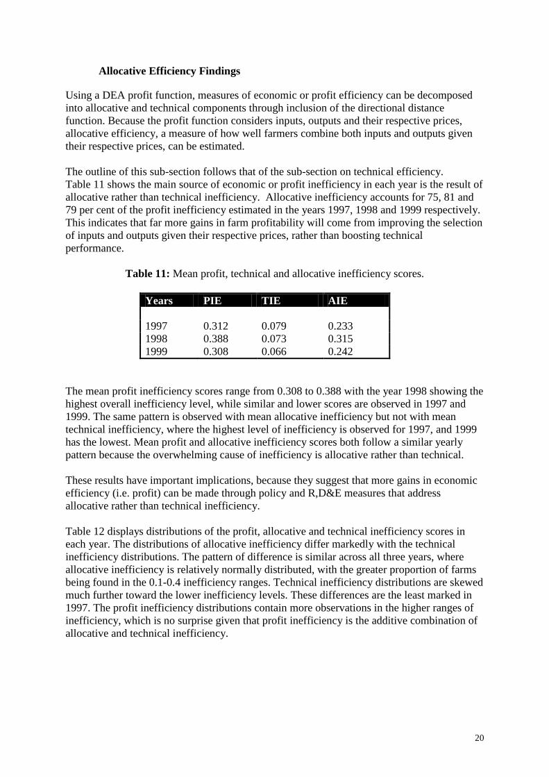
Allocative Efficiency Findings

Using a DEA profit function, measures of economic or profit efficiency can be decomposed

into allocative and technical components through inclusion of the directional distance

function. Because the profit function considers inputs, outputs and their respective prices,

allocative efficiency, a measure of how well farmers combine both inputs and outputs given

their respective prices, can be estimated.

The outline of this sub-section follows that of the sub-section on technical efficiency.

Table 11 shows the main source of economic or profit inefficiency in each year is the result of

allocative rather than technical inefficiency. Allocative inefficiency accounts for 75, 81 and

79 per cent of the profit inefficiency estimated in the years 1997, 1998 and 1999 respectively.

This indicates that far more gains in farm profitability will come from improving the selection

of inputs and outputs given their respective prices, rather than boosting technical

performance.

Table 11: Mean profit, technical and allocative inefficiency scores.

Years PIE TIE AIE

1997 0.312 0.079 0.233

1998 0.388 0.073 0.315

1999 0.308 0.066 0.242

The mean profit inefficiency scores range from 0.308 to 0.388 with the year 1998 showing the

highest overall inefficiency level, while similar and lower scores are observed in 1997 and

1999. The same pattern is observed with mean allocative inefficiency but not with mean

technical inefficiency, where the highest level of inefficiency is observed for 1997, and 1999

has the lowest. Mean profit and allocative inefficiency scores both follow a similar yearly

pattern because the overwhelming cause of inefficiency is allocative rather than technical.

These results have important implications, because they suggest that more gains in economic

efficiency (i.e. profit) can be made through policy and R,D&E measures that address

allocative rather than technical inefficiency.

Table 12 displays distributions of the profit, allocative and technical inefficiency scores in

each year. The distributions of allocative inefficiency differ markedly with the technical

inefficiency distributions. The pattern of difference is similar across all three years, where

allocative inefficiency is relatively normally distributed, with the greater proportion of farms

being found in the 0.1-0.4 inefficiency ranges. Technical inefficiency distributions are skewed

much further toward the lower inefficiency levels. These differences are the least marked in

1997. The profit inefficiency distributions contain more observations in the higher ranges of

inefficiency, which is no surprise given that profit inefficiency is the additive combination of

allocative and technical inefficiency.

21

Table 12: Inefficiency distributions in 1997, 1998 and 1999.

IE

Range

PIE

TIE

AIE PIE

TIE

AIE PIE

TIE

AIE

1997 1998 1999

0.0 3 33 3 1 37 1 2 36 2

0.0 – 0.1 6 23 15 6 26 8 7 34 16

0.1 – 0.2 19 29 29 9 21 20 24 14 34

0.2 – 0.3 20 6 9 13 8 27 21 6 14

0.3 – 0.4 18 2 8 26 1 12 15 3 10

0.4 – 0.5 12 5 17 10 11 8

0.5 – 0.6 11 2 6 5 1 3

0.6 – 0.7 3 6 3 6 2

0.7 – 0.8 5 4 3 1

0.8 – 0.9 1 1 1

0.9 – 1.0 1 1 1 1

1.0 – 1.1 1 1 2 2

1.1 – 1.2 1 1

Table 13 displays the changes in inputs and outputs that would be required for the average

farm to become economically efficient in each year. Looking first at outputs; to increase

economic efficiency, the average farm would have needed to increase its production of crops

in all three years, while increasing livestock production in two of the three years (1997 and

1998). In both 1997 and 1999, greater increases in the production of crops than livestock

needed to be made in order to maximise profits. These results are interesting, because in WA

and other Australian States, prices for sheep and wool have been in decline relative to crop

prices during the study period, 1997 to 1999. In response many farmers were shifting their

resource allocation from livestock to cropping enterprises. According to these results greater

changes in this direction were required if farmers during the period were to raise their profit

levels and attain economic efficiency.

Table 13: Changes in the levels of inputs and outputs necessary to achieve

economic efficiency for the average farm.

Crop Livestock Capital Labour Material

Services

1997

Original levels 2.250 0.799 0.961 0.773 1.035 1.425

EE levels

5.168 0.816 0.962 0.931 1.565 1.968

1998

Original levels 1.890 0.563 0.875 0.643 1.097 1.415

EE levels

5.086 0.390 1.043 0.573 1.716 2.019

1999

Original levels 2.547 0.438 0.700 0.720 1.267 0.862

EE levels

4.286 0.682 0.766 1.038 1.429 0.897

22

Overall, input usage increased in each year. This is not surprising, because, in order to

maximise profits much larger quantities of crops needed to be grown, which also entails

increasing the overall scale of production. While it is possible, it would take most farms some

years to alter both their production mix and scale of operation to the extent suggested by the

results in table 13. A proper practical perspective of the results is that they should relate more

to medium term suggested changes for the farm businesses than short-run changes. This is

partly due to the fact that all of the inputs in the model were treated as variable inputs.

However, in practice some of the inputs (e.g. capital) or components of the inputs are more

fixed in nature and so their alteration is more a medium term or long-run decision.

Are DEA efficiency rankings consistent?

To test if farms that perform well technically also perform well economically and allocatively,

Spearman coefficients of rank correlation were calculated. The hypothesis tested was:

H0: rs = 0, i.e. there is no significant correlation between the two series of ranks.

H1: rs ≠ 0, i.e. there is significant correlation between the two series of ranks.

Results are presented in table 14.

Table 14: Rank agreement between efficiency series.

Years rs t - test statistic Decision

1997

TIE vs PIE 0.414 4.340a Reject H0

TIE vs AIE -0.020 -0.192 Accept H0

PIE vs AIE 0.846 15.130a Reject H0

1998

TIE vs PIE 0.277 2.753a Reject H0

TIE vs AIE -0.109 -1.049 Accept H0

PIE vs AIE 0.872 17.024a Reject H0

1999

TIE vs PIE 0.386 3.994a Reject H0

TIE vs AIE -0.043 -0.410 Accept H0

PIE vs AIE 0.825 13.941a Reject H0

a and

b denote t-statistics significant at the 1 per cent and 5 per cent levels of significance.

The profit and allocative efficiency rankings are positively correlated at a very high level of

significance in each year. The technical efficiency rankings are also positively correlated with

profit efficiency rankings at a high level of significance in each year. However, there is no

significant correlation between technical and allocative efficiency in any of the years

examined.

These results indicate the top technical performers are different to the top allocative

performers. This finding has important implications for policy and R,D&E activities. If these

activities solely target technically inefficient farmers, they may be misguided where these

farms already display profit and allocative efficiency. Further, using R,D&E to solely

improve farmers' technical efficiency does not necessarily ensure improvement in their

allocative and profit efficiency; yet it appears that farmers have most to benefit from

improvement in these latter two.

23

Do ‘economically efficient’ farms remain efficient?

The stability of PIE and AIE ranks over time is assessed by calculation of Spearman

coefficients of rank correlation. Results are presented in Table 15. Again it is important, from

a policy and R,D&E point of view, to see whether or not the top performers in the sample can

be consistently identified from year to year. The statistical test for the following hypothesis

was the Spearman coefficient of rank correlation:

H0: rs = 0, i.e. there is no significant correlation between the two series of ranks.

H1: rs ≠ 0, i.e. there is significant correlation between the two series of ranks.

The efficiency rankings in each series were significantly similar across the consecutive years

1997-1998 and 1998-1999, as well across the three years, 1997-1999 at the 1 per cent level of

significance (see table 6.7). This is a positive result because it demonstrates that both the

directional distance function and profit efficiency DEA models consistently identify both

good and poor performers with regard to economic, technical and allocative efficiency.

Table 15: Rank agreement between inefficiency series over consecutive years,

1997 - 1998, and 1998 – 1999 and 1997 – 1999.

Years rs t - test statistic Decision

1997 – 1998

PIE 0.646 8.076a Reject H0

TIE 0.375 3.865a Reject H0

AIE 0.676 8.741a Reject H0

1998 – 1999

PIE 0.575 6.712a Reject H0

TIE 0.424 4.464a Reject H0

AIE 0.697 9.277a Reject H0

1997 – 1999

PIE 0.449 4.793a Reject H0

TIE 0.278 2.765a Reject H0

AIE 0.567 6.558a Reject H0

a denotes t-statistics significant at the 1 per cent level of significance.

The movement of ‘best-practice’ farms from one year to the next was also examined. Only

farms in the ‘efficient set’ (i.e. those fully efficient farms comprising the frontier) were

examined. The findings are limited because they do not reveal the magnitude of the decline

in efficiency of farms that move out of the efficient set. For example, a farm may move out of

the efficient set but still be relatively efficient, hence its overall rank won’t differ markedly.

None of the farms that were allocatively or economically efficient remained so after even a

single season. This is not surprising given that a maximum of 3 out 93 farms were found to be

fully efficient in any year. One reason why so few farms are found to be economically

efficient is because this is dependent not only on being efficient in production (i.e. being

technically efficient), but also on having an optimal combination of inputs and outputs given

their respective prices (i.e. being allocatively efficient). Also, a farmer’s potential to perform

24

well in an allocative capacity is likely to be confounded by yearly or seasonal variation in the

prices of inputs and outputs.

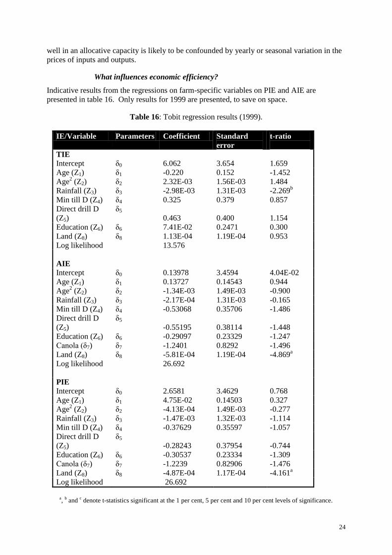
What influences economic efficiency?

Indicative results from the regressions on farm-specific variables on PIE and AIE are

presented in table 16. Only results for 1999 are presented, to save on space.

Table 16: Tobit regression results (1999).

IE/Variable Parameters Coefficient Standard

error

t-ratio

TIE

Intercept δ0 6.062 3.654 1.659

Age (Z1) δ1 -0.220 0.152 -1.452

Age2 (Z2) δ2 2.32E-03 1.56E-03 1.484

Rainfall (Z3) δ3 -2.98E-03 1.31E-03 -2.269b

Min till D (Z4) δ4 0.325 0.379 0.857

Direct drill D

(Z5)

δ5

0.463 0.400 1.154

Education (Z6) δ6 7.41E-02 0.2471 0.300

Land (Z8) δ8 1.13E-04 1.19E-04 0.953

Log likelihood 13.576

AIE

Intercept δ0 0.13978 3.4594 4.04E-02

Age (Z1) δ1 0.13727 0.14543 0.944

Age2 (Z2) δ2 -1.34E-03 1.49E-03 -0.900

Rainfall (Z3) δ3 -2.17E-04 1.31E-03 -0.165

Min till D (Z4) δ4 -0.53068 0.35706 -1.486

Direct drill D

(Z5)

δ5

-0.55195 0.38114 -1.448

Education (Z6) δ6 -0.29097 0.23329 -1.247

Canola (δ7) δ7 -1.2401 0.8292 -1.496

Land (Z8) δ8 -5.81E-04 1.19E-04 -4.869a

Log likelihood 26.692

PIE

Intercept δ0 2.6581 3.4629 0.768

Age (Z1) δ1 4.75E-02 0.14503 0.327

Age2 (Z2) δ2 -4.13E-04 1.49E-03 -0.277

Rainfall (Z3) δ3 -1.47E-03 1.32E-03 -1.114

Min till D (Z4) δ4 -0.37629 0.35597 -1.057

Direct drill D

(Z5)

δ5

-0.28243 0.37954 -0.744

Education (Z6) δ6 -0.30537 0.23334 -1.309

Canola (δ7) δ7 -1.2239 0.82906 -1.476

Land (Z8) δ8 -4.87E-04 1.17E-04 -4.161a

Log likelihood 26.692

a,

b and

c denote t-statistics significant at the 1 per cent, 5 per cent and 10 per cent levels of significance.

25

In 1999 land (Z8) was the only significant variable identified in regressions on both AIE and

PIE scores. Regressions on TIE in 1999 only identified one significant variable, rainfall. As

was the case in both 1997 and 1998, Z8 was significantly and positively related to AIE and

PIE at the 1 per cent level.

Drawing on the results from the regressions on the allocative efficiency scores across all years

(see Henderson 2002), there is evidence that direct drill D (Z5), minimum till D (Z4),

education (Z6) and land (Z8) all have a positive and significant effect on efficiency.

The results from the profit efficiency models tell a similar story, with land (Z8) having the

most consistent significant impact on economic efficiency. This result is almost entirely

related to its impact on allocative rather than technical inefficiency. In none of the three years

did canola (Z7) explain a significant amount of the variation in AIE or PIE. This suggests that

despite farmers receiving a historically high price for this crop over the period of this study,

and although its impact was positive, it did not significantly affect the profitability of these

farms.

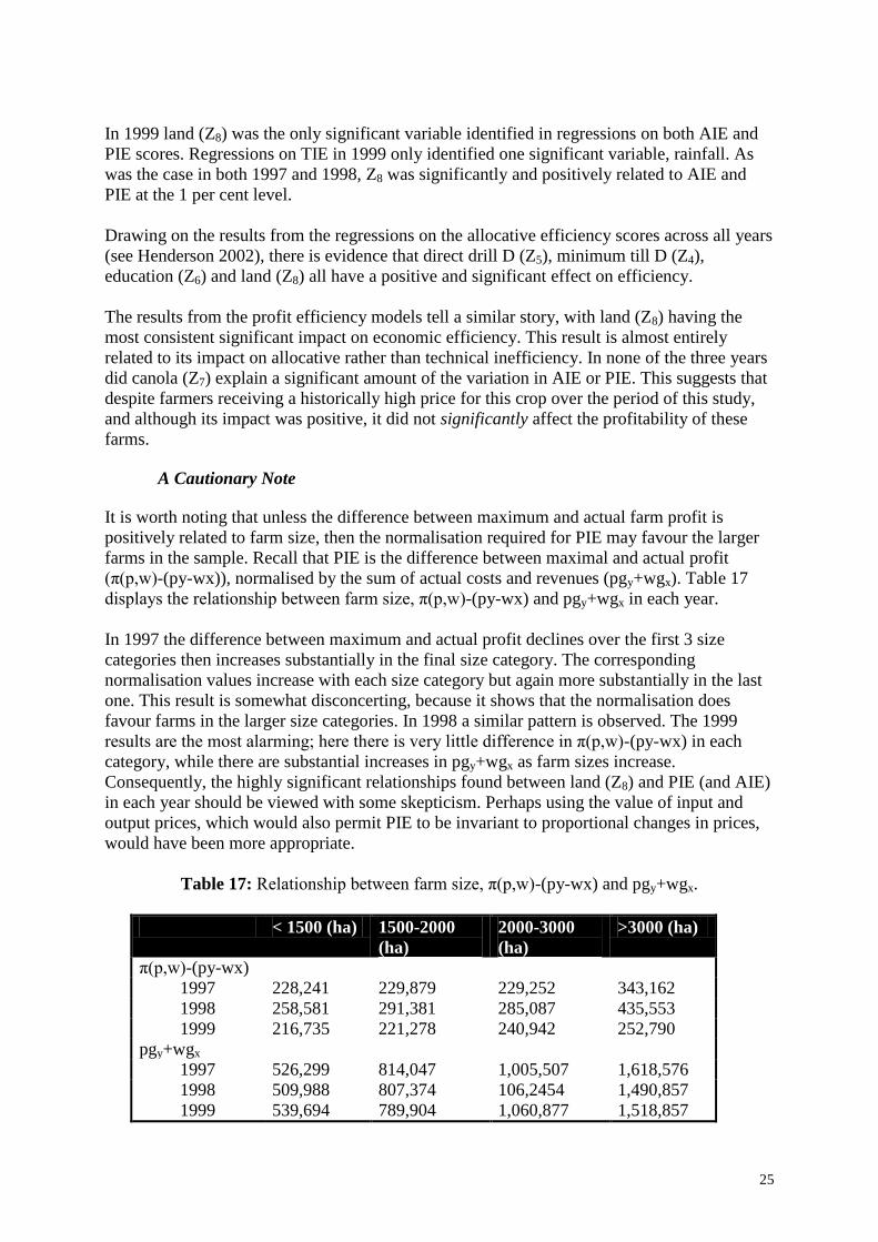
A Cautionary Note

It is worth noting that unless the difference between maximum and actual farm profit is

positively related to farm size, then the normalisation required for PIE may favour the larger

farms in the sample. Recall that PIE is the difference between maximal and actual profit

(π(p,w)-(py-wx)), normalised by the sum of actual costs and revenues (pgy+wgx). Table 17

displays the relationship between farm size, π(p,w)-(py-wx) and pgy+wgx in each year.

In 1997 the difference between maximum and actual profit declines over the first 3 size

categories then increases substantially in the final size category. The corresponding

normalisation values increase with each size category but again more substantially in the last

one. This result is somewhat disconcerting, because it shows that the normalisation does

favour farms in the larger size categories. In 1998 a similar pattern is observed. The 1999

results are the most alarming; here there is very little difference in π(p,w)-(py-wx) in each

category, while there are substantial increases in pgy+wgx as farm sizes increase.

Consequently, the highly significant relationships found between land (Z8) and PIE (and AIE)

in each year should be viewed with some skepticism. Perhaps using the value of input and

output prices, which would also permit PIE to be invariant to proportional changes in prices,

would have been more appropriate.

Table 17: Relationship between farm size, π(p,w)-(py-wx) and pgy+wgx.

< 1500 (ha) 1500-2000

(ha)

2000-3000

(ha)

>3000 (ha)

π(p,w)-(py-wx)

1997 228,241 229,879 229,252 343,162

1998 258,581 291,381 285,087 435,553

1999 216,735 221,278 240,942 252,790

pgy+wgx

1997 526,299 814,047 1,005,507 1,618,576

1998 509,988 807,374 106,2454 1,490,857

1999 539,694 789,904 1,060,877 1,518,857

26

Section 3: Concluding Remarks

An examination of mean technical efficiency scores using DEA and SFA revealed that

technical inefficiency in a southern agricultural region of Western Australia decreasing over

the years 1997 to 1999. A comparison of mean DEA and SFA scores revealed that the SFA

approach identified higher levels of technical inefficiency than the DEA approach. The

distributions of inefficiency revealed by each method were found to be heavily skewed

toward lower levels, becoming increasingly skewed over time as more farms moved closer to

the frontier.

To achieve technical efficiency the average farm was calculated to require its output levels to

increase by 6.4, 6.5 and 6.0 per cent in the years 1997, 1998 and 1999 respectively, while

input levels needed to be reduced by 16.4, 15.1 and 10.7 per cent in the same years. The

results indicated that most of this reduction is achievable through reducing the use of capital.

The SFA results, on the other hand, predict more optimistic estimates for potential gains in

output, which is not surprising given that it only considers the expansion of outputs and not

the contraction of inputs

Rank agreements between the DEA and SFA scores were assessed using Spearman

coefficients of rank correlation, and significant rank agreement was found between each series

in each year. This result should give practitioners the confidence that, regardless of which

method is employed, efficient farms can be identified.

The stability of the efficiency rankings identified by each approach over time also was

investigated. Spearman coefficients of rank correlation were used to assess the stability of

efficiency rankings over time. The ranks identified by DEA were more stable over time than

the SFA ranks. Results suggest that DEA is superior at identifying farms that persist in

technical efficiency. Conditional probabilities were also calculated to examine the durability

of farm efficiency. These results also indicated that DEA produced more temporally stable

efficiency rankings. It is also possible, however, that the farms’ relative efficiency levels vary

significantly from year to year and that the SFA approach reflects this.

The degree to which some farm specific factors can explain variation in technical efficiency

also was investigated using Tobit regressions. Farmers engaging in no-till cropping were less

efficient than those farmers reliant on minimum tillage practices to prepare seedbeds. This

suggests that at least a small amount of tillage produces benefits, such as pest control and

more rapid growth, that outweigh the improvements in soil sustainability and reduced time

and capital requirements that come with no-till farming (at least in the short term). Analysis of

the same variables to explain variation in the technical inefficiency effects in the SFA model

identified a different set of significant variables. This demonstrates that there is some

disparity between the scores from each method, despite their rankings being significantly

alike. Here, farm size, farmer age, education levels and rainfall were all found to be positively

and significantly related to technical efficiency. There was also some evidence to support the

life-cycle hypothesis; where farmer productivity increases first as middle age approaches and

then decreases again at a similar rate.

Although technical inefficiency declined consistently from 1997 to 1999, profit and allocative

inefficiency peaked in 1998, with 1997 and 1999 recording similar levels. The overwhelming

source of profit inefficiency was attributable to allocative rather than technical inefficiency.

This finding has important policy and R,D&E implications, because it suggests that policies

27

and R,D&E activities that target allocative rather than technical performance of farmers may

more effectively improve their profitability. One explanation for the poor allocative

performance of the sample firms is that because the prices of commodities and factors of

production are subject to yearly variation beyond the control of farm managers, it is often

more difficult to perform as well allocatively as it is technically. However, a valid alternative

explanation is simply that this finding is due to the restrictive nature of the analysis. When

there is little variation in farm prices, the DEA problem identifies very few allocatively

efficient points on the frontier.

There was no rank agreement found between the AIE and TIE rankings across the three years.

This also has important implications, because policies and R,D&E activities that target

technically inefficient farms may be somewhat misguided if these farms perform well in an

allocative capacity. The rankings of all three efficiency series were found to be stable over

time which demonstrates not only the persistence of characteristics (e.g. ‘best-practice’

management) that beneficially affect technical and allocative efficiency, but also that DEA is

a reliable technique for identifying this efficient set of farms.

Tobit regression results identified land and minimum tillage as two variables that explained

most of the variation in AIE across each year. Education and direct drill technology also had a

significant and positive impact on AIE in one of the three years. The findings on the impact of

crop establishment are interesting when viewed in conjunction with the results from the TIE

regressions, where no-till farming proved to have a significant positive relationship with TIE.

This latter finding suggests that the benefits, such as weed control and soil aeration,

associated with at least a minimum level of tillage, are more beneficial to productivity than

the benefits that come with no-till farming, e.g. reduced labour and soil improvement.

However, the evidence from this analysis suggests that both minimum tillage and no-tillage

operations are related to higher levels of allocative efficiency than conventional or multiple

tillage practices. This could be due to minimum and no-till farming practices requiring less

expensive items such as capital and labour, providing greater flexibility in crop sowing, and

also because they provide farmers with more time to focus on other areas of production.

Farm size was found to have a positive and consistent significant relationship with allocative

efficiency. However, as mentioned in the cautionary note, the normalisation underpinning the

PIE measure downwardly biases the inefficiency scores for larger farms. The gains from

rearrangement of inputs and outputs to achieve allocative efficiency should also be viewed

with caution because if a farm changes its proportion of inputs and outputs its level of

technical efficiency is also likely to change (Farrell 1957). In addition, because the production

mix of farms is often adjusted to expected future prices rather than actual prices, farms may

be identified as being inefficient when they are actually, in prospect at least, efficient.

28

Appendix One

Crops

The crops variable comprises an aggregation of seven crop types: wheat, barley, oats, lupins,

canola and other crops (such as faba beans and field peas). Crop prices could not be obtained

simply by deflating the value of crop sales by the quantity harvested, because not all of the

harvested quantity is sold in each year. Harvested crops are sold sequentially by commodity

boards, in a system known as pooling. Farmers receive a stream of payments, known as pool

payments, from the sale of their harvested grain. Although farmers receive the bulk of these

payments in the year following the harvest, these payments can extend over a few years.

Accordingly, crop prices are estimated as State cash-equivalent prices minus district freight

charges.

Livestock

The livestock quantity variable is an aggregate of sheep and cattle numbers and products sold.

However, very few farms in the sample run cattle enterprises. Beginning with the sheep

quantity variables, there are two different outputs: the first of these consists of sheep sold plus

any positive change in the livestock inventory. The second is the quantity of wool produced in

the production year.

The prices corresponding to these quantity variables were calculated in the following way: the

value of sheep sold was simply divided by the number of sheep sold. Positive changes in the

inventory between the beginning and end of the season were priced using the farm’s average

sale price of sheep sold that year. These are commonly referred to as positive operating gains.

Occasionally the value for wool sales listed on the farmer's balance sheet did not necessarily

match the quantities of wool produced, according to the farm physical record. This is because

wool is not always sold soon after shearing. It can be warehoused. Fortunately though, the

prices for wool sold directly by each farmer were available from the farmer records.

For cattle the only product is the number of cows sold. This output was computed in exactly

the same manner as for sheep, i.e. numbers sold plus positive operating gains.11

Capital

The capital variable is an aggregate of five items: land, buildings and structures, plant

(machinery and vehicles), sheep and cattle.

The first three of these five items were converted from stock into flow variables by

calculating their user costs. These variables were converted into user costs simply by taking

the average of their opening and closing values and multiplying this average by the market

real rate of interest for that year. Thus the user cost could be interpreted as the cost to the

farmer of not selling her on-farm assets and putting her money into a high interest savings

account.

11

Where there were no sales, and hence no prices available for cattle and sheep, average State prices from the

ABARE farm survey for that year were used.

29

The land item was classified as total hectares of land and its price was derived simply by

dividing its user cost by this quantity12

. Unfortunately it was not possible to separate buildings

and structures from land and hence, estimate depreciation on these items. Because they are

included in the land category, their cost is captured partly by the user cost of land. According

to ABARE statistics on the average WA broadacre farm, depreciation on buildings and

structures represents a much smaller fraction of costs than depreciation on plant (vehicles and

machinery) (ABARE 1999). Depreciation on plant items is included in the capital variable.

For the plant item the user cost was calculated following the approach outlined above and

then depreciation was added13

. This total value was then deflated using a price index taken

from ABARE’s annual farm survey results, to obtain quantity estimates. This price index

represents the average price for these items for WA farms in each year. Unfortunately,

applying this index necessitates the assumption that all farms have equal unit costs for these

items. This is an unavoidable distortion given that both quantity and price information are

required to calculate technical and allocative efficiency, respectively.

The livestock inputs, sheep and cattle comprise two components. The first is purchases plus

the absolute value of negative operating gains (i.e. when closing numbers less opening

numbers is negative), which can be interpreted as capital stock depletion to produce output.

Rather than using the purchase price to value the decrease in the livestock inventory, the sale

price for that year was used. This is because the average purchase price is usually inflated by

the purchase of rams that are considerably more expensive than ewes, lambs or wethers. The

second component of the livestock inputs is their user costs which are calculated by

multiplying the value of the opening numbers of livestock by the real rate of interest for the

relevant year.

Labour

The labour variable consisted of three items: operator/family labour, hired labour and

shearing expenses.

The farm records from which these variables were constructed contained information on the

number of weeks worked by the farm operator and family members. The market rate for

labour, obtained from ABARE farm survey results, was used as a notional price for

operator/family labour.

The numbers of weeks worked by hired employees was also recorded, along with money paid

in wages for hired labour. A price for hired labour was easily obtained by dividing wages paid

by the number of weeks worked.

Shearing expenses for each farm were taken from the farm financial records. Corresponding

quantity indexes for each year were drawn from ABARE’s annual farm survey results.

Materials

Materials is an aggregation of five items; crop chemicals, fodder and agistment, fertiliser,

seed, and fuel. Only costs were available for these items, and once again the average price

indices for these items were taken from ABARE survey results from WA broadacre farms and

12

Total land area rather than effective hectares was used. 13

A depreciation rate of 8 per cent was assumed to be appropriate. This was taken from the PlanFarm survey for

the 1999 year (pp. 26) (PlanFarm 2000).

30

were used to obtain quantity estimates by deflating their respective costs. By applying an

average price it was necessary, once more, to make the assumption that all the items were of

equal unit value and of homogenous quality.

Services

Like materials, the items that make up services are only reported as costs on the farm

financial records. The service cost items include: rates and taxes, administrative costs,

miscellaneous livestock costs, total contract costs, total repairs costs, net insurance costs,

other costs (e.g. general freight, fertiliser freight and spreading, electricity and gas). Again,

average price indices were taken from ABARE WA farm survey results and quantities were

obtained by deflating costs.

The materials and services variables are the least perfect because they make the assumption

that all farms face the same price for these inputs. The same is true of capital, but to a lesser

extent. Given the quality of the data available, these variables were seen to give the best

representation of the farm production structure. Ideally enterprise-specific variables should be

used to characterise the farm production processes. However, this was not possible given that

the farm records did not contain enterprise-specific input data. For example, the capital items

and overheads are not reported as enterprise specific inputs and can only be partitioned with

difficulty, and with the need to make further restrictive

A SFA production frontier based on a Cobb-Douglas functional form with two different

distributional assumptions is used to estimate technical efficiency effects. One assumes a

truncated-normal distribution, while the other assumes that the technical efficiency effects are

a linear function of a number of farm and farmer-specific variables. Hypothesis tests reveal

that the latter specification is preferred.

To answer this question, the technical performance of 93 broadacre farm businesses from

1997 to 1999 was examined using two new techniques, data envelopment analysis (DEA) and

stochastic frontier analysis (SFA). The main preliminary findings revealed that:

Most farms demonstrated high levels of technical efficiency.

Technical efficiency improved over the three years.

The distribution of technical efficiency among farms was uneven - of concern was the

small, yet diminishing portion of farms displaying relatively low levels of technical

efficiency.

Both analytical techniques, DEA and SFA, generated consistent rankings of farm

technical efficiency.

Farms identified as being very efficient tended to remain so.

A range of factors influenced technical efficiency, including rainfall, farm size, tillage

method, formal education level of the farmer, and their age.

The survey examined three types of farm efficiency, although only technical efficiency has

been reported on here. A business is technically efficient if its inputs cannot be reorganised to

generate more output. In a cropping context this would mean an efficient farmer has

combined his inputs such as machinery, labour, fertilisers and herbicides in such a way that he

achieves the maximum production possible in that season. A technically efficient farmer is

getting the maximum output from a given set of inputs.

31

References

ABARE (1999) “Australian Grains Industry: Performance by GRDC Agro-ecological Zones.”

Australian Bureau of Agricultural and Resource Economics, Canberra, pp. 144.

ABARE (2000) “Australian Grains Industry 2000.” Australian Farm Surveys Report 2000

Australian Bureau of Agricultural and Resource Economics, pp. 87.

ABARE/GRDC. “Productivity Achievements and Drivers of Change in the Grains Industry -

feed back from regional workshops.” Australian Bureau of Agricultural and Resource

Economics / Grains Research Development Corporation (1999).

Afriat, S. N. (1972) “Efficiency Estimation of Production Functions.” International Economic

Review 13: 568-598.

Aigner, D., K. Lovell, and P. Schmidt (1977) “Formulation and Estimation of Stochastic

Frontier Production Function Models.” Journal of Econometrics 6: 21-37.

Aigner, D. J., and S. F. Chu (1968) “On Estimating the Industry Production Function.”

American Economic Review 58: 826-839.

AWA (2000) “The Wheat Book: Principles and Practice.” Bulletin No. 4443. Agriculture

Western Australia, pp322.

Banker, R. (1989) “Econometric Estimation and Data Envelopment Analysis.” Research in

Governmental and Nonprofit Accounting 5: 231-243.

Banker, R. (1996) “Hypothesis Tests Using Data Envelopment Analysis.” The Journal of

Productivity Analysis 7: 139-159.

Banker, R. D., A. Charnes, and W. W. Cooper (1984) “Some Models for Estimating

Technical and Scale Inefficiencies in Data Envelopment Analysis.” Management

Science 30, no. 9: 1078-1092.

Battese, G., and T. Coelli (1988) “Prediction of Firm-Level Technical Efficiencies with a

Generalised Frontier Production Function and Panel Data.” Journal of Econometrics

38: 387-399.

Battese, G., and G. Corra (1977) “Estimation of a Production Frontier Model: with

Application to the Pastoral Zone of Eastern Australia.” Australian Journal

Agricultural Economics 21: 169-179.

Bligh, K., and P. Findlater (1996) “No-till sowing: helping to keep cropland soils in place.”

Journal of Agriculture (Western Australia) 37, no. 2(1996): 50-55.

Chambers, R. G. (2000) “Efficiency in Agriculture: Where Should We Look?” Working

Paper. Department of Economics, Unversity of Maryland, College Park, October 18.

Chapman, L., V. Roriguez, and S. Harrison (1999) “Influence of Resource Quality on

Productivity of Wool Producing Farms.” Australian Farm Surveys Report: 37-41.

Charnes, A., W. Cooper, and E. Rhodes (1978) “Measuring the Efficiency of Decision

Making Units.” European Journal of Operational Research 2: 429-444.

Coelli, T. (1995) “Recent Developments in Frontier Modelling and Efficiency Measurement.”

Department of Econometrics, University of New England, Armidale, NSW 2531

Australia.

Coelli, T. (1996) “A guide to FRONTIER version 4.1: a computer program for stochastic

frontier an cost function estimation.” The University of New England (UNE).

Coelli, T., P. Rao, and G. Battese (1998) An Introduction to Efficiency and Productivity

Analysis: Kluwer Academic Publishers.

DAWA (1991) “The Wheat Book: A Technical Manual for Wheat Producers.” WA

Department of Agriculture Bulletin 4196, pp. 182.

Elteto, O. and P. Koves (1964) “On a problem of Index Number Computation Relating to

International Comparison.” Statisztikai Szemle, 42: 507-518.

32

Färe, R., S. Grosskopf, and C.A.K. Lovell (1985), The Measurement of Efficiency of

Production, Kluwer Academic Publishers, Boston.

Farrell, M. (1957) “The measurement of productive efficiency.” Journal of the Royal

Statistical Society 120: 253-81.

Fernandez-Cornejo, J. (1994) “Nonradial Technical Efficiency and Chemical Input use in

Agriculture.” Agricultural and Resource Economics Review 23, no. 1: 11-21.

Ferrier, G., and C. Lovell (1990) “Measuring Cost Efficiency in Banking.” Journal of

Econometrics 46: 229-245.

Fraser, I., and D. Cordina (1999) “An application of data envelopment analysis to irrigated

dairy farms in Northern Victoria, Australia.” Agricultural Systems 59: 267-282.

Fraser, I., and P. Hone (2001) “Farm-level efficiency and productivity measurement using

panel data: wool production in south-west Victoria.” The Australian Journal of

Agricultural and Resource Economics 45, no. 2: 215-232.

Greene, W. H. (1980) “On the Estimation of a Flexible Frontier Production Model.” Journal

of Econometrics 13: 27-56.

Ha, A., and L. Chapman (2000) “Productivity growth trends across Australian broadacre

industries.” Australian Commodities 7, no. 2: 334-240.

Henderson, B. (2002) “Efficiency in Western Australian Broadacre Agriculture: A

Comparison Between Data Envelopment Analysis and Stochastic Frontier Analysis.”

Unpublished M.Sc. thesis, School of Agricultural and Resource Economics,

University of Western Australia.

Hjalmarsson, L., S. Kumbhakar, and A. Heshmati (1996) “DEA, DFA and SFA: A

Comparison.” The Journal of Productivity Analysis 7: 303-327.

Jondrow, J., C. Lovell, I. Materov and P. Schmidt (1982) “On the Estimation of Technical

Inefficiency in the Stochastic Frontier Production Function Model.” Journal of

Econometrics 19: 233-238.

Kalaitzandonakes, N., and E. Dunn (1995) “Technical Efficiency, Managerial Ability and

Farmer Education in Guatemalan Corn Production: A Latent Variable Analysis.”

Agricultural and Resource Economics Review 24: 36-46.

Kalaitzandonakes, N. G., W. Shunxiang, and M. Jian-chun (1992) “The Relationship between

Technical Efficiency and Firm Size Revisited.” Canadian Journal of Agricultural

Economics 40: 427-442.

Kumbhakar, S., S. Ghosh, and J. McGuckin (1991) “A Generalised Production Frontier

Approach for Estimating Determinants of Inefficiency in U.S. Dairy Farms.” Journal

of Business and Economic Statistics 9, no. 3: 279-286.

Meeusen, W., and J. van den Broeck (1977) “Efficiency Estimation from Cobb-Douglas

Production Functions with Composed Error.” International Economic Review 18: 435-

444.

PlanFarm (2000) “PlanFarm survey for the 1999 year.” West Perth, PlanFarm.

Reifshneider, D., and R. Stevenson (1991) “Systematic Departures From the Frontier: A

Framework for the Analysis of Firm Inefficiency.” International Economic Review 32,

no. 3: 715-723.

Stevenson, R. (1980) “Likelihood Functions for Generalised Stochastic Frontier Estimation.”

Journal of Econometrics 13: 57-66.

Szulc, B.J. (1964) “Indices for Multiregional Comparisons.” Prezeglad Statystyczny

(Statistical Review) 3:239-254.

Tauer, L. (1984) “Productivity of Farmers at Various Ages.” North Central Journal of

Agricultural Economics 6, no. 1: 81-87.

Tauer, L. (1995) “Age and farmer productivity.” Review of Agricultural Economics 17: 63-69.

33

Thomas, A., and L. Tauer (1994) “Linear Input Aggregation Bias in Nonparametric Technical

Efficiency Measurement.” Canadian Journal of Agricultural Economics 42: 77-86.