AN INVESTIGATION OF PRODUCE COOLING TUNNEL …

AN INVESTIGATION OF PRODUCE COOLING TUNNEL PERFORMANCE

Martins J.P and Rankin G.W*. *Author for correspondence

Department of Mechanical, Automotive and Materials Engineering, University of Windsor,

Windsor, ON, Canada N9B 3P4, E-mail: [email protected]

ABSTRACT The numerical results from a simple computational fluid

dynamic model of a forced air agricultural produce cooling tunnel are compared with experimental measurements made on a full scale tunnel. The experimental tunnel consists of four pallets of produce each holding a number of boxes arranged in a specified, but non-uniform stacking order. The tunnel is located in a large cold storage room while the cold air is drawn at a steady rate through the boxes using a large axial flow fan. The time dependent temperature and pressure values are experimentally determined at a number of strategic locations within the tunnel. The experimentally determined values of the tunnel pressures as well as the produce temperature as functions of time are plotted in a non-dimensional manner. These are then compared with the results of the computational fluid dynamics model. In the model the boxes filled with the agricultural produce, cucumbers in this case, are approximated using porous jumps for the boxes and a non-isotropic porous media model with empirically determined coefficients for the produce. A commercially available finite volume package is used to solve for the time dependent temperature, pressure and flow field. The discrepancies between the experimental and numerical results are discussed and suggestions made for improving the numerical model.

NOMENCLATURE

P [Pa] Pressure t [hrs] Time T [C] Temperature

Special characters � [-] Non-dimensional temperature

Subscriptsinitial Value at beginning of cooling room Room value 0 Ambient or reference

INTRODUCTION According to Bronson [1] the fact that cooling of

agricultural produce within a short period of time after harvest is an extremely important factor in achieving a high quality product with long shelf life was first reported in 1904. The longer shelf life is a result of the slower respiration rate and metabolism which occurs at lower temperatures. Post-harvest cooling also results in lower wilting, reduced amounts of mould and bacteria as well as less ethylene production.

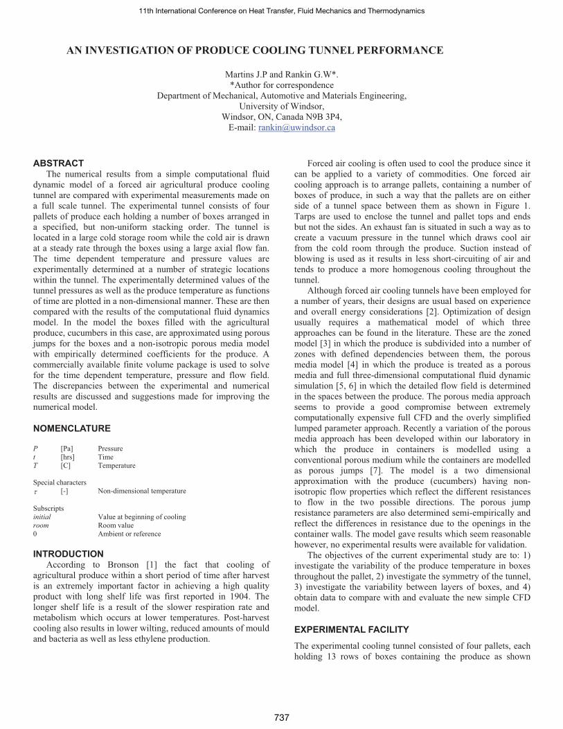
Forced air cooling is often used to cool the produce since it can be applied to a variety of commodities. One forced air cooling approach is to arrange pallets, containing a number of boxes of produce, in such a way that the pallets are on either side of a tunnel space between them as shown in Figure 1. Tarps are used to enclose the tunnel and pallet tops and ends but not the sides. An exhaust fan is situated in such a way as to create a vacuum pressure in the tunnel which draws cool air from the cold room through the produce. Suction instead of blowing is used as it results in less short-circuiting of air and tends to produce a more homogenous cooling throughout the tunnel.

Although forced air cooling tunnels have been employed for a number of years, their designs are usual based on experience and overall energy considerations [2]. Optimization of design usually requires a mathematical model of which three approaches can be found in the literature. These are the zoned model [3] in which the produce is subdivided into a number of zones with defined dependencies between them, the porous media model [4] in which the produce is treated as a porous media and full three-dimensional computational fluid dynamic simulation [5, 6] in which the detailed flow field is determined in the spaces between the produce. The porous media approach seems to provide a good compromise between extremely computationally expensive full CFD and the overly simplified lumped parameter approach. Recently a variation of the porous media approach has been developed within our laboratory in which the produce in containers is modelled using a conventional porous medium while the containers are modelled as porous jumps [7]. The model is a two dimensional approximation with the produce (cucumbers) having non-isotropic flow properties which reflect the different resistances to flow in the two possible directions. The porous jump resistance parameters are also determined semi-empirically and reflect the differences in resistance due to the openings in the container walls. The model gave results which seem reasonable however, no experimental results were available for validation.

The objectives of the current experimental study are to: 1) investigate the variability of the produce temperature in boxes throughout the pallet, 2) investigate the symmetry of the tunnel, 3) investigate the variability between layers of boxes, and 4) obtain data to compare with and evaluate the new simple CFD model.

EXPERIMENTAL FACILITY The experimental cooling tunnel consisted of four pallets, each holding 13 rows of boxes containing the produce as shown

11th International Conference on Heat Transfer, Fluid Mechanics and Thermodynamics

737

schematically in Figure 1. In this experiment the containers were filled with produce consisting of medium cucumbers. Two of the pallets are visible in Figure 1 and will be referred to as the pallets on the right while the other two are on the far side of the tunnel (pallets on the left) with a one pallet space between the left and right pallets to form the tunnel space. The top is covered with a tarp and the end walls were constructed using plywood with an angle iron frame. A 24 inch diameter, direct drive, cast aluminium propeller wall fan with 8 blades with a propeller blade angle of 24 degrees (Twin City WPD-24E8-24) was used to draw air from the tunnel space between the pallets. A by-pass door, not visible in the figure was installed in the plywood back wall in order to control the tunnel pressure. A foam seal was inserted around and between the boxes of produce in order to minimize the by-pass (short circuiting) of air.

Figure 1 Schematic Diagram of Experimental Cooling Tunnel

Figure 2 Experimental Cooling Tunnel in Cold Room

The experimental produce cooling tunnel was contained in a large (21.5 m long by 11 m wide and 5 m high) cool room. The

room was kept cool by four large refrigeration units as shown in Figure 2.

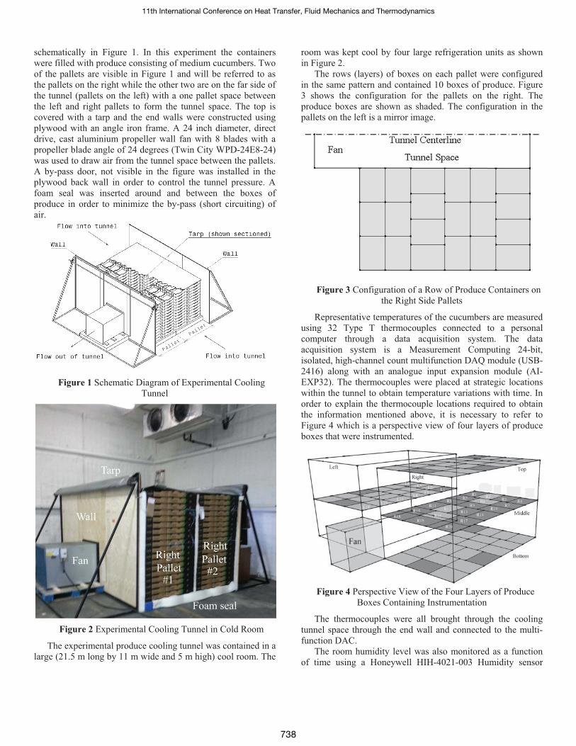
The rows (layers) of boxes on each pallet were configured in the same pattern and contained 10 boxes of produce. Figure 3 shows the configuration for the pallets on the right. The produce boxes are shown as shaded. The configuration in the pallets on the left is a mirror image.

Figure 3 Configuration of a Row of Produce Containers on the Right Side Pallets

Representative temperatures of the cucumbers are measured using 32 Type T thermocouples connected to a personal computer through a data acquisition system. The data acquisition system is a Measurement Computing 24-bit, isolated, high-channel count multifunction DAQ module (USB-2416) along with an analogue input expansion module (AI-EXP32). The thermocouples were placed at strategic locations within the tunnel to obtain temperature variations with time. In order to explain the thermocouple locations required to obtain the information mentioned above, it is necessary to refer to Figure 4 which is a perspective view of four layers of produce boxes that were instrumented.

Figure 4 Perspective View of the Four Layers of Produce Boxes Containing Instrumentation

The thermocouples were all brought through the cooling tunnel space through the end wall and connected to the multi-function DAC.

The room humidity level was also monitored as a function of time using a Honeywell HIH-4021-003 Humidity sensor


738

connected to the analogue input channel of the multi-purpose DAC.

The pressure within selected boxes were measured using a handheld electronic manometer (Omega Model HHP-103) connected to Tygon tubing. The other end of the tubing was situated within the box of produce so that the tube end was not in a high velocity region.

EXPERIMENTAL PROCEDURE Once the cucumbers had been instrumented, the tarp

covering was installed and any locations of airflow by-pass filled with a foam sealing material. The data acquisition equipment was then connected and the initial values of the thermocouple readings taken as well as the room humidity reading. The tunnel fan was then started and an initial set of produce box pressure readings taken. This was repeated approximately every hour of testing. The thermocouple and humidity values were recorded at five second intervals for approximately four hours. As preliminary measurements indicated that the pressure levels within the boxes did not change with time they were measured approximately every 30 minutes in order to ensure that the tunnel flow conditions had not changed throughout the cooling period The overall testing time was restricted due to the fact that testing was done during the normal working hours in a fully functioning produce handling facility. It should also be mentioned that other activities such as fork-lift and personnel movement was ongoing during the testing period which may have had a minor effect on the results.

EXPERIMENTAL RESULTS The variation of the initial cucumber temperatures

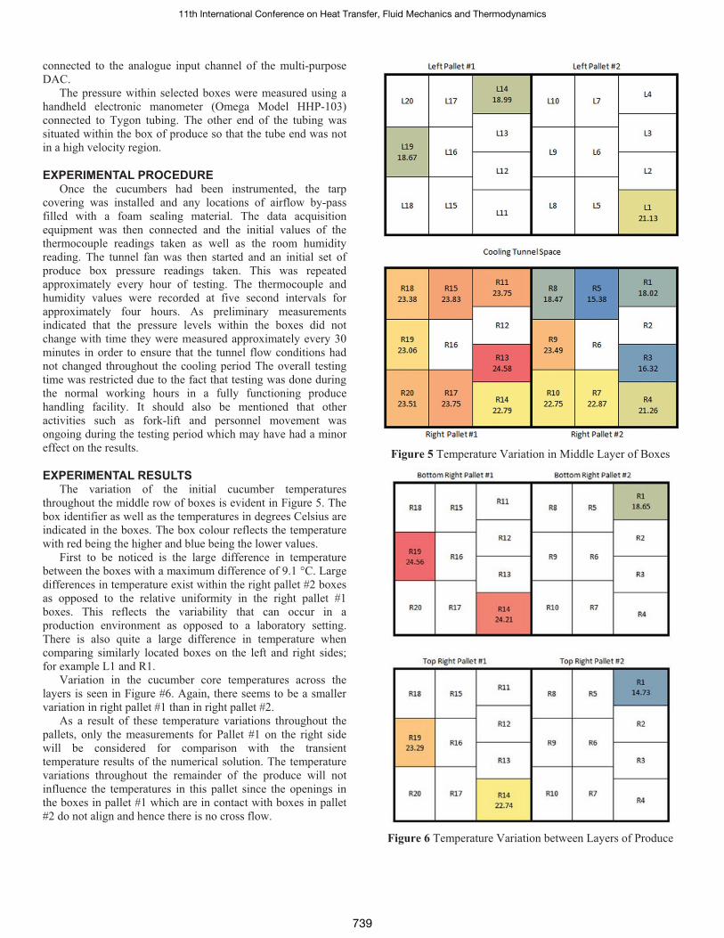
throughout the middle row of boxes is evident in Figure 5. The box identifier as well as the temperatures in degrees Celsius are indicated in the boxes. The box colour reflects the temperature with red being the higher and blue being the lower values.

First to be noticed is the large difference in temperature between the boxes with a maximum difference of 9.1 °C. Large differences in temperature exist within the right pallet #2 boxes as opposed to the relative uniformity in the right pallet #1 boxes. This reflects the variability that can occur in a production environment as opposed to a laboratory setting. There is also quite a large difference in temperature when comparing similarly located boxes on the left and right sides; for example L1 and R1.

Variation in the cucumber core temperatures across the layers is seen in Figure #6. Again, there seems to be a smaller variation in right pallet #1 than in right pallet #2.

As a result of these temperature variations throughout the pallets, only the measurements for Pallet #1 on the right side will be considered for comparison with the transient temperature results of the numerical solution. The temperature variations throughout the remainder of the produce will not influence the temperatures in this pallet since the openings in the boxes in pallet #1 which are in contact with boxes in pallet #2 do not align and hence there is no cross flow.

Figure 5 Temperature Variation in Middle Layer of Boxes

Figure 6 Temperature Variation between Layers of Produce


739

Variation of the temperature of the produce and the room with time will be presented and discussed in connection with the description of the numerical model and its results.

Likewise, the experimental pressure values will be presented as a comparison with the predicted numerical values. The relative humidity in the room remained approximately constant ranging from approximately 90 to 95%.

NUMERICAL MODEL The numerical model used to predict the cooling tunnel

performance is a modification of that presented in our previous paper [7]. The model is a two-dimensional, incompressible flow approximation. Porous jumps are used to model the boxes while a non-isotropic porous media is used to model the produce in each box. The necessary flow constants for those materials are determined in the same empirical manner as described in the previous paper. The heat transfer model has been changed slightly to include a more accurate approximation for the Nusselt number a low Reynolds numbers and the configuration of the boxes on the pallets is also different in this case.

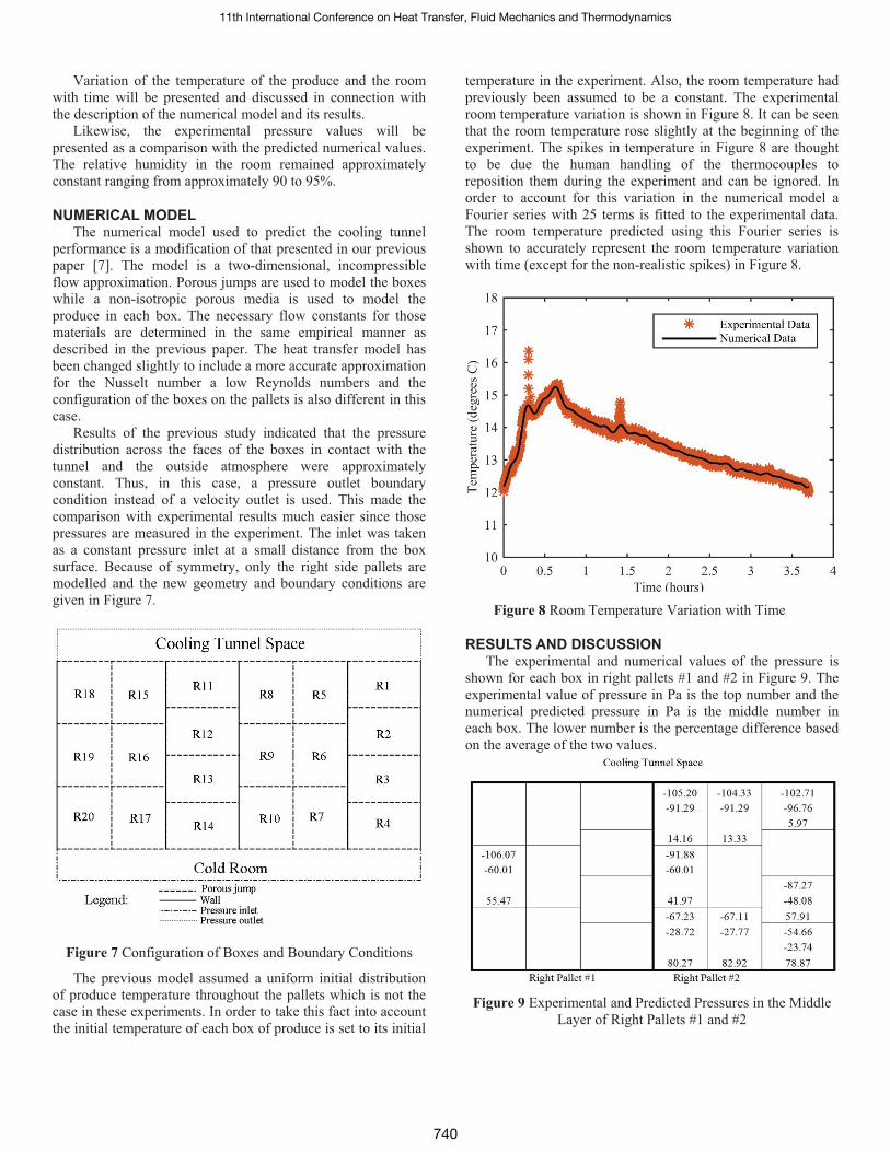
Results of the previous study indicated that the pressure distribution across the faces of the boxes in contact with the tunnel and the outside atmosphere were approximately constant. Thus, in this case, a pressure outlet boundary condition instead of a velocity outlet is used. This made the comparison with experimental results much easier since those pressures are measured in the experiment. The inlet was taken as a constant pressure inlet at a small distance from the box surface. Because of symmetry, only the right side pallets are modelled and the new geometry and boundary conditions are given in Figure 7.

Figure 7 Configuration of Boxes and Boundary Conditions

The previous model assumed a uniform initial distribution of produce temperature throughout the pallets which is not the case in these experiments. In order to take this fact into account the initial temperature of each box of produce is set to its initial

temperature in the experiment. Also, the room temperature had previously been assumed to be a constant. The experimental room temperature variation is shown in Figure 8. It can be seen that the room temperature rose slightly at the beginning of the experiment. The spikes in temperature in Figure 8 are thought to be due the human handling of the thermocouples to reposition them during the experiment and can be ignored. In order to account for this variation in the numerical model a Fourier series with 25 terms is fitted to the experimental data. The room temperature predicted using this Fourier series is shown to accurately represent the room temperature variation with time (except for the non-realistic spikes) in Figure 8.

Figure 8 Room Temperature Variation with Time

RESULTS AND DISCUSSION The experimental and numerical values of the pressure is

shown for each box in right pallets #1 and #2 in Figure 9. The experimental value of pressure in Pa is the top number and the numerical predicted pressure in Pa is the middle number in each box. The lower number is the percentage difference based on the average of the two values.

Figure 9 Experimental and Predicted Pressures in the Middle Layer of Right Pallets #1 and #2


740

Although pressures were measured in boxes located within the left pallets and in the top and bottom right pallets, they are not shown graphically in order to conserve space. The maximum variation between boxes with similar locations throughout the pallets was found to be approximately 7%.

The more interesting result is the comparison of the predicted pressures with the experimentally observed values. Although the maximum differences are quite large a definite trend can be seen. The differences increase with distance from the cooling tunnel space. It is speculated that this difference is due to leakage of air between the plywood tunnel walls and the boxes as well as between the two pallets. Although foam was used to seal this space where the boxes meet the cold room air, it is possible for the space between the wall and the boxes to achieve a negative pressure and cause flow out the sides of the boxes and into the small space in which they are in contact. This would result in higher flow rates being drawn into the boxes adjacent to the cold room air giving a larger pressure drop in the porous jump next to the cold room. Various means of proving this hypothesis are currently being investigated, however, it is interesting to determine what effect this discrepancy has on the temperature results.

The comparison of the predicted temperatures with the experimental results is presented in two graphs in order to prevent overcrowding. The temperatures are plotted using a non-dimensional parameter defined as follows:

� �� roominitial

room

TTTtT��

�� (1)

, where T(t)is the time varying temperature, Troom is the lowest room temperature recorded and Tinitial is the initial temperature of the particular cucumber.

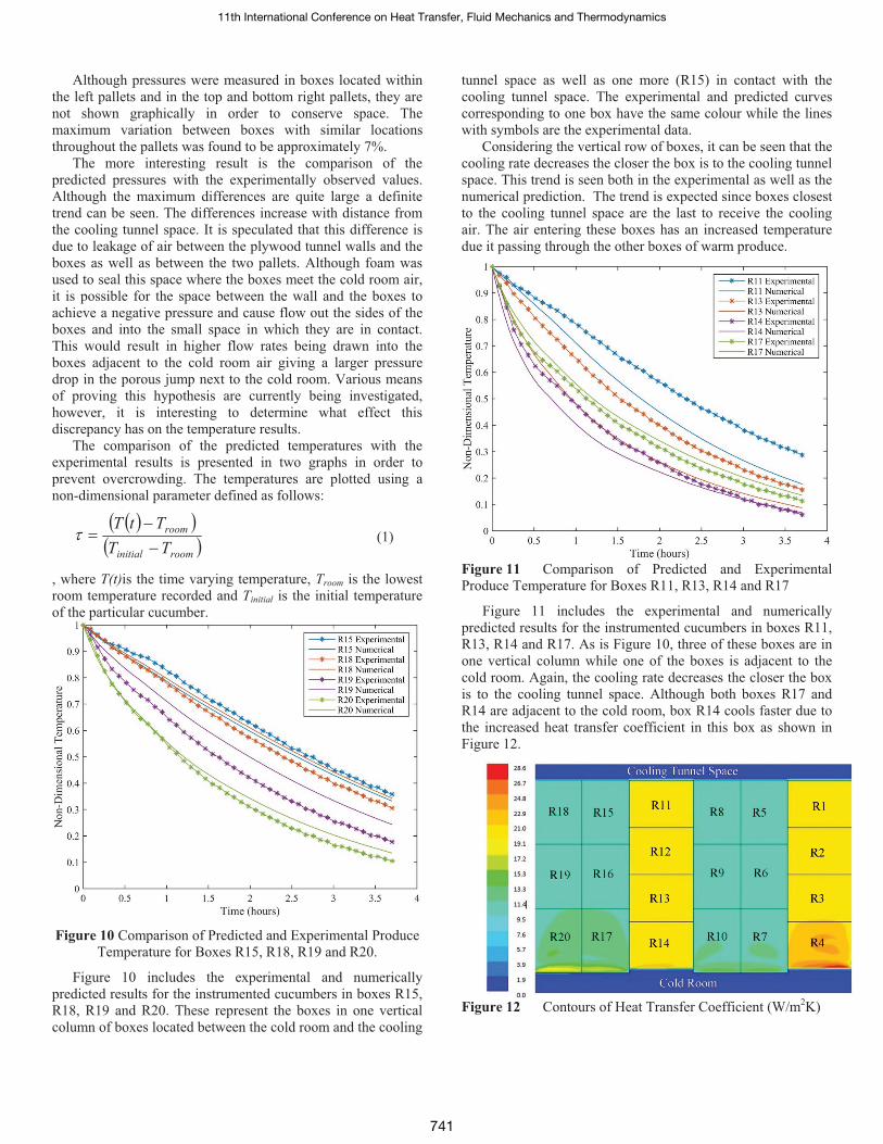
Figure 10 Comparison of Predicted and Experimental Produce Temperature for Boxes R15, R18, R19 and R20.

Figure 10 includes the experimental and numerically predicted results for the instrumented cucumbers in boxes R15, R18, R19 and R20. These represent the boxes in one vertical column of boxes located between the cold room and the cooling

tunnel space as well as one more (R15) in contact with the cooling tunnel space. The experimental and predicted curves corresponding to one box have the same colour while the lines with symbols are the experimental data.

Considering the vertical row of boxes, it can be seen that the cooling rate decreases the closer the box is to the cooling tunnel space. This trend is seen both in the experimental as well as the numerical prediction. The trend is expected since boxes closest to the cooling tunnel space are the last to receive the cooling air. The air entering these boxes has an increased temperature due it passing through the other boxes of warm produce.

Figure 11 Comparison of Predicted and Experimental Produce Temperature for Boxes R11, R13, R14 and R17

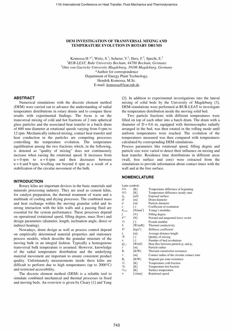
Figure 11 includes the experimental and numerically predicted results for the instrumented cucumbers in boxes R11, R13, R14 and R17. As is Figure 10, three of these boxes are in one vertical column while one of the boxes is adjacent to the cold room. Again, the cooling rate decreases the closer the box is to the cooling tunnel space. Although both boxes R17 and R14 are adjacent to the cold room, box R14 cools faster due to the increased heat transfer coefficient in this box as shown in Figure 12.

Figure 12 Contours of Heat Transfer Coefficient (W/m2K)


741

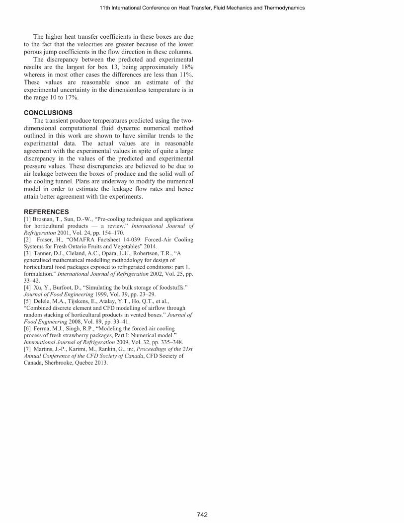
The higher heat transfer coefficients in these boxes are due to the fact that the velocities are greater because of the lower porous jump coefficients in the flow direction in these columns.

The discrepancy between the predicted and experimental results are the largest for box 13, being approximately 18% whereas in most other cases the differences are less than 11%. These values are reasonable since an estimate of the experimental uncertainty in the dimensionless temperature is in the range 10 to 17%.

CONCLUSIONS The transient produce temperatures predicted using the two-

dimensional computational fluid dynamic numerical method outlined in this work are shown to have similar trends to the experimental data. The actual values are in reasonable agreement with the experimental values in spite of quite a large discrepancy in the values of the predicted and experimental pressure values. These discrepancies are believed to be due to air leakage between the boxes of produce and the solid wall of the cooling tunnel. Plans are underway to modify the numerical model in order to estimate the leakage flow rates and hence attain better agreement with the experiments.

REFERENCES [1] Brosnan, T., Sun, D.-W., “Pre-cooling techniques and applications for horticultural products — a review.” International Journal of Refrigeration 2001, Vol. 24, pp. 154–170. [2] Fraser, H., “OMAFRA Factsheet 14-039: Forced-Air Cooling Systems for Fresh Ontario Fruits and Vegetables” 2014. [3] Tanner, D.J., Cleland, A.C., Opara, L.U., Robertson, T.R., “A generalised mathematical modelling methodology for design of horticultural food packages exposed to refrigerated conditions: part 1, formulation.” International Journal of Refrigeration 2002, Vol. 25, pp. 33–42.[4] Xu, Y., Burfoot, D., “Simulating the bulk storage of foodstuffs.” Journal of Food Engineering 1999, Vol. 39, pp. 23–29. [5] Delele, M.A., Tijskens, E., Atalay, Y.T., Ho, Q.T., et al., “Combined discrete element and CFD modelling of airflow through random stacking of horticultural products in vented boxes.” Journal of Food Engineering 2008, Vol. 89, pp. 33–41. [6] Ferrua, M.J., Singh, R.P., “Modeling the forced-air cooling process of fresh strawberry packages, Part I: Numerical model.” International Journal of Refrigeration 2009, Vol. 32, pp. 335–348. [7] Martins, J.-P., Karimi, M., Rankin, G., in:, Proceedings of the 21st Annual Conference of the CFD Society of Canada, CFD Society of Canada, Sherbrooke, Quebec 2013.


742

DEM INVESTIGATION OF TRANSVERSAL MIXING AND

TEMPERATURE EVOLUTION IN ROTARY DRUMS

Komossa H.*1; Wirtz, S.

1; Scherer, V.

1; Herz, F.

2; Specht, E.

2

1RUB-LEAT, Ruhr University Bochum, 44780 Bochum, Germany 2Otto von Guericke University Magdeburg, 39106 Magdeburg, Germany

*Author for correspondence

Department of Energy Plant Technology,

Hendrik Komossa, M.Sc.

E-mail: [email protected]

ABSTRACT

Numerical simulations with the discrete element method

(DEM) were carried out to advance the understanding of radial

temperature distributions in rotary drums and to compare these

results with experimental findings. The focus is on the

transversal mixing of cold and hot fractions of 2 mm spherical

glass particles and the associated heat transfer in a batch drum

of 600 mm diameter at rotational speeds varying from 0 rpm to

12 rpm. Mechanically induced mixing, contact heat transfer and

heat conduction in the particles are competing processes

controlling the temperature evolution. The temperature

equilibration among the two fractions which, in the following,

is denoted as “quality of mixing” does not continuously

increase when raising the rotational speed. It increases from

u = 0 rpm to u = 6 rpm and then decreases between

u = 6 and 9 rpm, levelling out beyond 6 rpm as a result of a

stabilization of the circular movement of the bulk.

INTRODUCTION

Rotary kilns are important devices in the basic materials and

minerals processing industry. They are used as cement kilns,

for catalyst preparation, the thermal treatment of waste and a

multitude of cooling and drying processes. The combined mass

and heat exchange within the moving granular solid and its

strong interaction with the kiln walls and a passing fluid are

essential for the system performance. These processes depend

on operational (rotational speed, filling degree, mass flow) and

design parameters (diameter, length, inclination angle, direct or

indirect heating).

Nowadays, drum design as well as process control depend

on empirically determined material properties and stationary

process models, which describe the granular structure of the

moving bulk in an integral fashion. Typically a homogenous

transversal bulk temperature is assumed. However, knowledge

of the radial temperature distribution and the underlying

material movement are important to ensure consistent product

quality. Unfortunately measurements inside these kilns are

difficult to perform due to high temperatures (up to 2000°C)

and restricted accessibility.

The discrete element method (DEM) is a reliable tool to

simulate combined mechanical and thermal processes in fixed

and moving beds. An overview is given by Cleary [1] and Yang

[2]. In addition to experimental investigations into the lateral

mixing of solid beds by the University of Magdeburg [3],

DEM-simulations were performed at RUB-LEAT to investigate

the temperature distribution inside the moving solid bed.

Two particle fractions with different temperatures were

filled on top of each other into a batch drum. The drum with a

diameter of D = 0.6 m, equipped with thermocouples radially

arranged in the bed, was then rotated in the rolling mode until

uniform temperatures were reached. The evolution of the

temperatures measured was then compared with temperatures

calculated by corresponding DEM simulations.

Process parameters like rotational speed, filling degree and

particle size were varied to detect their influence on mixing and

heat transfer. Residence time distributions in different areas

(wall, free surface and core) were extracted from the

simulations to provide information about contact times with the

wall and at the free surface.

NOMENCLATURE

Latin symbols ∆T0 [K] Temperature difference at beginning ∆T∞ [K] Temperature difference steady state

Ag [m²] Exposed surface

D [m] Drum diameter

d [m] Particle diameter

e [-] Coefficient of restitution

Ey,hm [N/mm2] Young’s modulus

f [%] Filling degree

Fn,t [N] Normal and tangential force vector

Fr [-] Froude-number k [W/m/K] Thermal conductivity

kn,t [kg/s2] Stiffness coefficient

lg [m] Average distance length M [-] Quality of mixing n [-] Number of bed revolutions

Q1,2 [W/m²] Heat flux between particle p1 and p2

r [m] Particle radius

Rc [K/W] Thermal constriction resistance

rc [m] Contact radius of the circular contact zone

Rg [K/W] Stagnant gas zone resistance

Tcf [K] Temperature cold fraction Thf [K] Temperature hot fraction TSurf [K] Surface temperature u [1/min] Rotational speed


743

Greek symbols

Θ [-] Poission’s ration

µG,dyn [-] Dynamic coefficient of friction

µH [-] Static coefficient of friction

µR [-] Coefficient of rolling friction

ρ [kg/m3] Density

ξ [m] Displacement, overlap

γn,t [kg/s] Damping coefficient

NUMERICAL METHOD AND SIMULATION SET-UP

Numerical method

In a discrete description (DEM), the movement of each

single particle in the bed is described by simultaneous

integration of Newton’s and Euler’s equations while

incorporating all interactions among the particles, the wall and

free surfaces. The discrete element code of LEAT [4], [5], [6]

was used in this study to simulate the rotating drum with

spherical particles. The particles are considered as soft spheres.

The linear spring dashpot model is used for normal and

tangential forces.

�� =�� + �� = �− � ∙ � − �� ∙ �� ∙ � (1)

�� =−��| � ∙ ��|, �� ∙ �� ∙ � (2)

To allow for particle rolling both translational and rotational

motion are resolved. Further details on the mechanical models

used may be found in [7].

For a detailed description of heat transfer in the moving

bulk, several heat transfer mechanisms must be considered.

According to Yagi and Kunii [8] seven different heat transfer

mechanisms are present in a packed bed, which can be divided

into heat transfer mechanisms independent of fluid flow:

1) Thermal conduction within solid particle

2) Thermal conduction through the contact surfaces of two

particles

3) Radiant heat transfer between surfaces of two particles

and heat transfer mechanisms depending on fluid flow:

4) Thermal conduction through the fluid film near the contact

surface of two particles

5) Heat transfer by convection, solid-fluid-solid

6) Heat transfer by lateral mixing of fluid

The relevant heat transfer mechanisms 1), 2) and 4) are

described within the DEM-code and will be presented in the

following. The modelling of contact heat transfer between

particles and conduction through interstitial gas (mechanism 2)

and 5)) is based on the approach by Vargas and McCarthy [9].

Here the classical elasticity theory of Hertz [10] is used to

calculate the contact area between two particles. The heat flux

induced by these two mechanisms is calculated by:

��,� = 1"# +1"$% ∙ ('()*,� − '()*,�) (3)

Both fluxes act in parallel and are governed by the same

difference of two particle surface temperatures. The thermal

constriction resistance (direct particle contact) Rc is

"# = 12 ∙ -. ∙ /# (4)

with contact radius rc of the circular contact zone:

/# = 3 ∙ (1 − 1-.� ) ∙ |��| ∙ /-.2 ∙ 2�,-. %�3 (5)

Fn is the normal force vector acting between the two

contacting particles. Ey,hm, rhm, θhm and khm are the harmonic

mean values of Young’s modulus, sphere radius, poission’s

ratio and thermal conductivity of the two particles in contact

calculated by the following equation:

4-. = 2 ∙ 4� ∙ 4�4� + 4� 5��ℎ4 ∈ 2� , /, 1, (6)

The heat flux across the stagnant gas zone around the

particle contact area

"$ = 8$ $ ∙ 9$ (7)

is computed with the exposed surface Ag and the average

distance lg:

9$ = 2 ∙ : ∙ /� − : ∙ /#� (8)

8$ = /-.� ∙ ;1 − :4=/-. − /# (9)

Validation of DEM Model

This model of contact heat transfer and conduction through

interstitial gas (among the particles and between particles and

the walls) was implemented in the DEM-Code and will be

validated in the following. The mechanical movement was

analysed by an investigation of the characteristic parameters for

the rotating drum system. These parameters are the Froude-

number, the dynamic angle of repose, the thickness of the

active layer and the particle velocity on the bed surface and at

the wall and were computed in DEM-simulations, measured in

rotating drum experiments and compared with each other [11].

The mechanical movement of a moving bed in rotating drums

can be described with DEM simulations with good accuracy in

the rolling and slumping bed motion.

Heat transfer was simulated and experimentally determined

in a batch drum filled with glass spheres (dP = 2 mm; f = 20 %)

by heating the outer wall of the drum to maximum temperatures

of TWall = 473.15 K, this is why radiation can be safely

neglected in this experimental set-up. For a detailed analysis of

heat transfer without any influence of bed movement (rolling

motion effects good transversal mixing, slumping motion

effects poor transversal mixing) experiments and simulations

were also carried out without any rotation of the drum


744

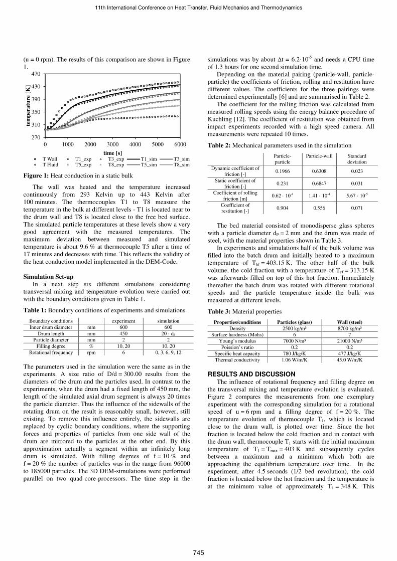
(u = 0 rpm). The results of this comparison are shown in Figure

1.

Figure 1: Heat conduction in a static bulk

The wall was heated and the temperature increased

continuously from 293 Kelvin up to 443 Kelvin after

100 minutes. The thermocouples T1 to T8 measure the

temperature in the bulk at different levels - T1 is located near to

the drum wall and T8 is located close to the free bed surface.

The simulated particle temperatures at these levels show a very

good agreement with the measured temperatures. The

maximum deviation between measured and simulated

temperature is about 9.6 % at thermocouple T5 after a time of

17 minutes and decreases with time. This reflects the validity of

the heat conduction model implemented in the DEM-Code.

Simulation Set-up

In a next step six different simulations considering

transversal mixing and temperature evolution were carried out

with the boundary conditions given in Table 1.

Table 1: Boundary conditions of experiments and simulations

Boundary conditions experiment simulation

Inner drum diameter mm 600 600

Drum length mm 450 20 · dP

Particle diameter mm 2 2

Filling degree % 10, 20 10, 20

Rotational frequency rpm 6 0, 3, 6, 9, 12

The parameters used in the simulation were the same as in the

experiments. A size ratio of D/d = 300.00 results from the

diameters of the drum and the particles used. In contrast to the

experiments, when the drum had a fixed length of 450 mm, the

length of the simulated axial drum segment is always 20 times

the particle diameter. Thus the influence of the sidewalls of the

rotating drum on the result is reasonably small, however, still

existing. To remove this influence entirely, the sidewalls are

replaced by cyclic boundary conditions, where the supporting

forces and properties of particles from one side wall of the

drum are mirrored to the particles at the other end. By this

approximation actually a segment within an infinitely long

drum is simulated. With filling degrees of f = 10 % and

f = 20 % the number of particles was in the range from 96000

to 185000 particles. The 3D DEM-simulations were performed

parallel on two quad-core-processors. The time step in the

simulations was by about ∆t = 6.2·10-5

and needs a CPU time

of 1.3 hours for one second simulation time.

Depending on the material pairing (particle-wall, particle-

particle) the coefficients of friction, rolling and restitution have

different values. The coefficients for the three pairings were

determined experimentally [6] and are summarised in Table 2.

The coefficient for the rolling friction was calculated from

measured rolling speeds using the energy balance procedure of

Kuchling [12]. The coefficient of restitution was obtained from

impact experiments recorded with a high speed camera. All

measurements were repeated 10 times.

Table 2: Mechanical parameters used in the simulation

Particle-

particle

Particle-wall Standard

deviation

Dynamic coefficient of

friction [-] 0.1966 0.6308 0.023

Static coefficient of

friction [-] 0.231 0.6847 0.031

Coefficient of rolling

friction [m] 0.62 · 10-4 1.41 · 10-4 5.67 · 10-5

Coefficient of

restitution [-] 0.904 0.556 0.071

The bed material consisted of monodisperse glass spheres

with a particle diameter dP = 2 mm and the drum was made of

steel, with the material properties shown in Table 3.

In experiments and simulations half of the bulk volume was

filled into the batch drum and initially heated to a maximum

temperature of Thf = 403.15 K. The other half of the bulk

volume, the cold fraction with a temperature of Tcf = 313.15 K

was afterwards filled on top of this hot fraction. Immediately

thereafter the batch drum was rotated with different rotational

speeds and the particle temperature inside the bulk was

measured at different levels.

Table 3: Material properties

Properties/conditions Particles (glass) Wall (steel)

Density 2500 kg/m³ 8700 kg/m³

Surface hardness (Mohs) 6 7

Young’s modulus 7000 N/m³ 21000 N/m³

Poission’s ratio 0.2 0.2

Specific heat capacity 780 J/kg/K 477 J/kg/K

Thermal conductivity 1.06 W/m/K 45.0 W/m/K

RESULTS AND DISCUSSION

The influence of rotational frequency and filling degree on

the transversal mixing and temperature evolution is evaluated.

Figure 2 compares the measurements from one exemplary

experiment with the corresponding simulation for a rotational

speed of u = 6 rpm and a filling degree of f = 20 %. The

temperature evolution of thermocouple T1, which is located

close to the drum wall, is plotted over time. Since the hot

fraction is located below the cold fraction and in contact with

the drum wall, thermocouple T1 starts with the initial maximum

temperature of T1 = Tmax = 403 K and subsequently cycles

between a maximum and a minimum which both are

approaching the equilibrium temperature over time. In the

experiment, after 4.5 seconds (1/2 bed revolution), the cold

fraction is located below the hot fraction and the temperature is

at the minimum value of approximately T1 = 348 K. This

270

310

350

390

430

470

0 1000 2000 3000 4000 5000 6000

tem

per

atu

re

[K]

time [s]T Wall T1_exp T3_exp T1_sim T3_simT Fluid T5_exp T8_exp T5_sim T8_sim


745

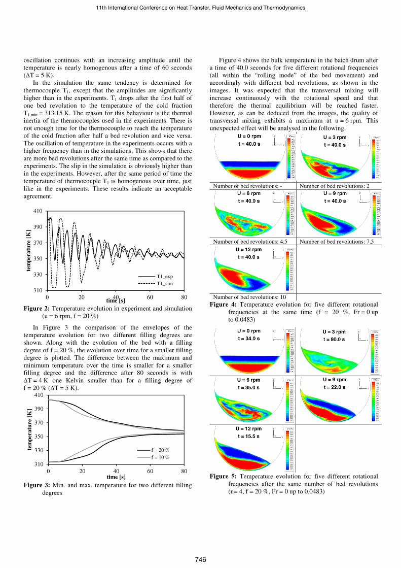
oscillation continues with an increasing amplitude until the

temperature is nearly homogenous after a time of 60 seconds

(∆T = 5 K).

In the simulation the same tendency is determined for

thermocouple T1, except that the amplitudes are significantly

higher than in the experiments. T1 drops after the first half of

one bed revolution to the temperature of the cold fraction

T1,min = 313.15 K. The reason for this behaviour is the thermal

inertia of the thermocouples used in the experiments. There is

not enough time for the thermocouple to reach the temperature

of the cold fraction after half a bed revolution and vice versa.

The oscillation of temperature in the experiments occurs with a

higher frequency than in the simulations. This shows that there

are more bed revolutions after the same time as compared to the

experiments. The slip in the simulation is obviously higher than

in the experiments. However, after the same period of time the

temperature of thermocouple T1 is homogenous over time, just

like in the experiments. These results indicate an acceptable

agreement.

Figure 2: Temperature evolution in experiment and simulation

(u = 6 rpm, f = 20 %)

In Figure 3 the comparison of the envelopes of the

temperature evolution for two different filling degrees are

shown. Along with the evolution of the bed with a filling

degree of f = 20 %, the evolution over time for a smaller filling

degree is plotted. The difference between the maximum and

minimum temperature over the time is smaller for a smaller

filling degree and the difference after 80 seconds is with

∆T = 4 K one Kelvin smaller than for a filling degree of

f = 20 % (∆T = 5 K).

Figure 3: Min. and max. temperature for two different filling

degrees

Figure 4 shows the bulk temperature in the batch drum after

a time of 40.0 seconds for five different rotational frequencies

(all within the “rolling mode” of the bed movement) and

accordingly with different bed revolutions, as shown in the

images. It was expected that the transversal mixing will

increase continuously with the rotational speed and that

therefore the thermal equilibrium will be reached faster.

However, as can be deduced from the images, the quality of

transversal mixing exhibits a maximum at u = 6 rpm. This

unexpected effect will be analysed in the following.

Number of bed revolutions: - Number of bed revolutions: 2

Number of bed revolutions: 4.5 Number of bed revolutions: 7.5

Number of bed revolutions: 10

Figure 4: Temperature evolution for five different rotational

frequencies at the same time (f = 20 %, Fr = 0 up

to 0.0483)

Figure 5: Temperature evolution for five different rotational

frequencies after the same number of bed revolutions

(n= 4, f = 20 %, Fr = 0 up to 0.0483)

310

330

350

370

390

410

0 20 40 60 80

tem

per

atu

re

[K]

time [s]

T1_exp

T1_sim

310

330

350

370

390

410

0 20 40 60 80

tem

per

atu

re

[K]

time [s]

f = 20 %

f = 10 %


746

The quality of transversal mixing increases with the

rotational speed from u = 0 rpm up to 6 rpm and the number of

bed revolutions from n = 0 up to n = 4.5 at 6 rpm. However, the

mixing quality decreases when raising the rotational speed

further (to u = 12 rpm) as shown in Figure 4. The computed

temperatures after the same number of bed revolutions, thus at

different (thermal relaxation) times, are presented by Figure 5.

Best thermal equalization is observed at the smallest rotational

frequency (u = 3 rpm), since in this case heat conduction, due

to the long time, has clearly a larger influence than the

mechanical mixing of particles. For the thermal properties

considered here, the thermal equalization is dominated by the

bulk mixing; equalization by conduction is much slower.

Again, as in Figure 4, the case with u = 6 rpm exhibits the

best spatial mixing, a result which requires further evaluation.

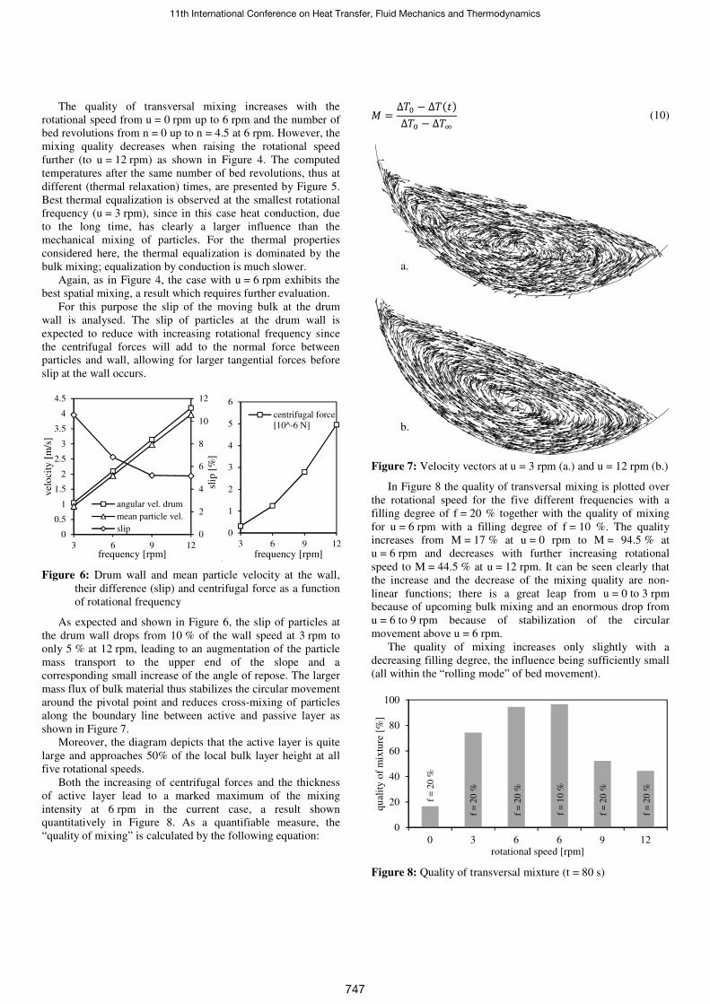
For this purpose the slip of the moving bulk at the drum

wall is analysed. The slip of particles at the drum wall is

expected to reduce with increasing rotational frequency since

the centrifugal forces will add to the normal force between

particles and wall, allowing for larger tangential forces before

slip at the wall occurs.

Figure 6: Drum wall and mean particle velocity at the wall,

their difference (slip) and centrifugal force as a function

of rotational frequency

As expected and shown in Figure 6, the slip of particles at

the drum wall drops from 10 % of the wall speed at 3 rpm to

only 5 % at 12 rpm, leading to an augmentation of the particle

mass transport to the upper end of the slope and a

corresponding small increase of the angle of repose. The larger

mass flux of bulk material thus stabilizes the circular movement

around the pivotal point and reduces cross-mixing of particles

along the boundary line between active and passive layer as

shown in Figure 7.

Moreover, the diagram depicts that the active layer is quite

large and approaches 50% of the local bulk layer height at all

five rotational speeds.

Both the increasing of centrifugal forces and the thickness

of active layer lead to a marked maximum of the mixing

intensity at 6 rpm in the current case, a result shown

quantitatively in Figure 8. As a quantifiable measure, the

“quality of mixing” is calculated by the following equation:

> = ∆'@ − ∆'(�)∆'@ − ∆'A (10)

Figure 7: Velocity vectors at u = 3 rpm (a.) and u = 12 rpm (b.)

In Figure 8 the quality of transversal mixing is plotted over

the rotational speed for the five different frequencies with a

filling degree of f = 20 % together with the quality of mixing

for u = 6 rpm with a filling degree of f = 10 %. The quality

increases from M = 17 % at u = 0 rpm to M = 94.5 % at

u = 6 rpm and decreases with further increasing rotational

speed to M = 44.5 % at u = 12 rpm. It can be seen clearly that

the increase and the decrease of the mixing quality are non-

linear functions; there is a great leap from u = 0 to 3 rpm

because of upcoming bulk mixing and an enormous drop from

u = 6 to 9 rpm because of stabilization of the circular

movement above u = 6 rpm.

The quality of mixing increases only slightly with a

decreasing filling degree, the influence being sufficiently small

(all within the “rolling mode” of bed movement).

Figure 8: Quality of transversal mixture (t = 80 s)

0

2

4

6

8

10

12

0

0.5

1

1.5

2

2.5

3

3.5

4

4.5

3 6 9 12

slip

[%

]

vel

oci

ty [

m/s

]

frequency [rpm]

angular vel. drum

mean particle vel.

slip0

1

2

3

4

5

6

3 6 9 12

frequency [rpm]

centrifugal force

[10^-6 N]

0

20

40

60

80

100

0 3 6 6 9 12

qu

alit

y o

f m

ixtu

re [

%]

rotational speed [rpm]

a.

b.

f =

10

%

f =

20

%

f =

20

%

f =

20

%

f =

20

%

f =

20

%


747

CONCLUSION

In the current study numerical simulations with the discrete

element method (DEM) were carried out to advance the

understanding of radial temperature distributions in rotary

drums, to compare these results with experimental findings and

to identify the influence of rotational speed and filling degree.

The simulations were conducted in a drum of D = 600 mm with

glass particles of dP = 2 mm just as in the experiments. The

rotational speed varied from u = 0 rpm to u = 12 rpm

(Fr = 0 to 0.0483) and filling degrees from f = 10 % to 20 %. A

cold and a hot fraction of particles were layered on each other

in the drum and the drum was rotated.

To remove the influence of the sidewalls, they were

replaced by cyclic boundary conditions, where the supporting

forces and properties of particles from one sidewall of the drum

are mirrored to the particles at the other end. By this

approximation actually a segment within an infinitely long

drum is simulated.

The heat conduction model was implemented in the LEAT-

DEM-Code and validated by heating a static bulk in the drum.

This verification reflects the validity of the heat conduction

model implemented in the LEAT-DEM-Code.

A comparison of the temperature evolution in the

experiment with the simulation (u = 6 rpm, f = 20 %) indicates

an acceptable agreement. However, the temperature amplitudes

in the simulation are significantly higher than in the

experiments; thermal inertia of the thermocouples used in the

experiments is a reason for that. The oscillation of temperature

in the experiments occurs with a higher frequency than in the

simulations since the slip in the simulation is higher. The

temperature, however, is uniform after the same period of time.

The quality of mixing increases only slightly with a

decreasing filling degree; all simulations were performed in the

“rolling mode”.

The quality of mixing does not increase steadily with

increasing rotational speed, as was expected. The quality

increases from u = 0 rpm to u = 6 rpm and the decreases with

further rising rotational speed. It can be seen clearly that there

is a great leap from u = 0 to 3 rpm due to upcoming bulk

mixing and an enormous drop from u = 6 to 9 rpm because of

stabilization of the circular movement above u = 6 rpm by

centrifugal forces.

In a further step different drum and particle diameters will

be simulated to investigate the influence on transversal

movement and consequently on the quality of mixing by

variation of the acting centrifugal forces.

ACKNOWLEDGEMENT

The current study has been funded by the German Research

Foundation (Deutsche Forschungsgemeinschaft, DFG) within

the project SPP 1679 SCHE 322/11-1 and by the German

Federation of Industrial Research Associations (AiF) within the

project AiF 17133 BG/2. The authors would like to

acknowledge the generous support.

REFERENCES

[1] P.W. Cleary, DEM prediction of industrial and geophysical particle flows, Particuology 8, 106-118

(2010)

[2] R.Y. Yang, A.B. Yu, L. McElroy, J. Bao, Numerical simulation of particle dynamics in different flow regimes in a rotating drum, Powder Technology 188,

170-177 (2008)

[3] A.I. Nafsun, F. Herz, E. Specht, H. Komossa, S. Wirtz,

V. Scherer, Experimental Investigation of the Thermal Bed Mixing in Rotary Drums, Conference Paper,

HEFAT 2015

[4] H. Kruggel-Emden, E. Simsek, S. Rickelt, S. Wirtz, V.

Scherer, Review and extension of normal force models for the Discrete Element Method, Powder Technology

171, 157–173 (2007)

[5] H. Kruggel-Emden, S. Wirtz, V. Scherer, A study on tangential force laws applicable to the discrete element method (DEM) for materials with viscoelastic or plastic behaviour, Chemical Engineering Science 63, 1523–

1541 (2008)

[6] D. Höhner, S. Wirtz, V. Scherer, Experimental and numerical investigation on the influence of particle shape and shape approximation on hopper discharge using the discrete element method, Powder Technology

235, 614-627 (2012)

[7] F. Sudbrock, E. Simsek, S. Wirtz, V. Scherer, An experimental analysis on mixing and stoking of monodisperse spheres on a grate, Powder Technology

198 (2010) 29–37

[8] S. Yagi, D. Kunii, Studies on effective thermal conductivities in packed beds, AIChE J. 3, 373–381

(1957)

[9] W.L. Vargas, J. McCarthy, Conductivity of granular media with stagnant interstitial fluids via thermal particle dynamics simulation, Int. J. Heat Mass Transf.

45 (2002) 4847–4856.

[10] H. Hertz, Über die Berührung fester elastischer Körper,

J. Für Die Reine Und Angew. Mech. 92, 156–171

(1881)

[11] H. Komossa; S. Wirtz; V. Scherer; F. Herz; E. Specht:

Transversal bed motion in rotating drums using spherical particles: Comparison of experiments with DEM simulations, Powder Technology 264, 96-104,

014

[12] H. Kuchling, Taschenbuch der Physik, Fachbuchverlag

Leipzig, 17. Auflage (2004)


748

A DYNAMIC PROCESS MODEL FOR A SIDEWELL FURNACE

Kocaefe Y.*, Bui R.T., Charette A.

*Author for correspondence

Department of Applied Sciences,

University of Quebec at Chicoutimi

555, boul. de l’Université, Chicoutimi, Quebec, Canada G7H 2B1


ABSTRACT

Today, aluminum is used in many applications due to its

many desirable properties such as lightweight, high resistance

to corrosion, excellent conduction of heat and electricity, high

ductility, and easy recyclability. Canada is one of the top

aluminum producing and exporting countries in the world; and

this is due to its high hydro-electric power generation capacity.

Production of aluminum through recycling requires much less

energy compared to the primary aluminum production, i.e.,

starting from the raw materials. This has a positive impact on

the environment as well.

Different types of furnaces are used to melt the recycled

aluminum. Sidewell furnaces are usually used for the melting

of recycled beverage cans. The sidewell furnaces have a side

well (as the name implies) in addition to the main chamber. The

chips are fed to the side well, and the metal circulates between

the two parts of the furnace to carry out the melting. A dynamic

process model has been developed for such furnaces. This

model consists of two parts: one sub-model for the combustion

chamber and one sub-model for the liquid metal. Unlike other

dynamic process models, this approach converts the metal flow

calculated in 3D using CFX (now ANSYS-CFX) into a

simplified flow field and integrates it into the model. Thus, the

process model accounts for the impact of the flow field as well.

In this article, the dynamic process model will be

explained, including the above novel approach to incorporate

the flow field in a simplified model. The results of a number of

case studies will be presented, which demonstrate the

application of the model as well as the effectiveness of the

approach used for taking into account the detailed flow field.

INTRODUCTION Aluminum production has been increasing steadily for

the past number of decades due to its many desirable properties.

Canada is, with about 7% of world production, one of the major

aluminum producing and exporting countries. Due to the

electrical energy production using hydro power, it produces the

‘greenest aluminium’, that is, the aluminium production with the lowest environmental imprint in the world.

Aluminium produced starting with the raw materials is

called the primary aluminum. This requires the electrolysis of

cryolite at high temperatures (around 950C), which is a highly

energy-intensive process. Secondary aluminium is the

aluminium produced from the recycled metal. Aluminium can

be recycled almost infinitely. This route requires about 5-8% of

the energy needed for the primary aluminium production,

excluding the energy used in the transportation of recycled

NOMENCLATURE CP [Jkg-1 C -1] Heat capacity

k [W m-1 C-1] Thermal conductivity

m [kg s-1] Mass flow rate

Q [W] Heat flow rate

T [C or K] Temperature

t [s] Time

V [m3] Volume

x [m] Spatial coordinate

Special characters

ρ [kg m-3] Density

α [m s-2] Thermal diffusivity

Subscripts

in Property entering a cell

out Property leaving a cell

metal. There are numerous benefits of recycling: conservation

of energy and resources as well as reduction in environmental

emissions and cost [1].

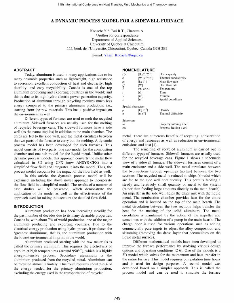
The remelting of recycled aluminum is carried out in

different types of furnaces. Sidewell furnaces are usually used

for the recycled beverage cans. Figure 1 shows a schematic

view of a sidewell furnace. The sidewell furnaces consist of a

main enclosure and a side well. The metal circulates between

the two sections through openings (arches) between the two

sections. The recycled metal is reduced to chips (shreds) which

are fed to the side well continuously. This permits feeding a

steady and relatively small quantity of metal to the system

(rather than feeding large amounts directly to the main hearth).

An impeller in the side well helps the chips mix with the liquid

metal. The combustion chamber provides heat for the entire

operation and is located on the top of the main hearth. The

metal circulation between the two sections helps transfer the

heat for the melting of the solid aluminum. The metal

circulation is maintained by the action of the impeller and

sometimes with the addition of a pump in the main hearth. The

charge door is used for various operations such as adding

commercially pure ingots to adjust the alloy composition and

skimming (removing the dross layer that accumulates on the

liquid metal surface).

Different mathematical models have been developed to

improve the furnace performance by studying various design

options and operating conditions [2-6]. One of the models is a

3D model which solves for the momentum and heat transfer in

the entire furnace. This model requires computation time hours

and is used for design purposes. A second model was

developed based on a simpler approach. This is called the

process model and can be used to simulate the furnace


749

mailto:[email protected]

operation. The latter model runs in a few minutes and allows

the study of the impact of various operational parameters on the

furnace performance rapidly. Each model has its utility.

Figure 1 A schematic view of a sidewell furnace

Both models have been developed using a modular

structure: one sub-model for the metal part and a second sub-

model for the combustion chamber. These two parts of the

furnace have distinctively different characteristics; thus, the

modular approach simplifies the model development. Also, the

sub-models can be used exclusively for particular studies on

each part. The models account for all the important phenomena

occurring in the furnace.

Normally, no flow calculation is done in the process

models to keep them simple, and the flow is either neglected or

included using an approximate representation. However, in the

current process model, the flow field determined by the 3D

model has been incorporated into the process model by

simplifying the complex flow pattern and adapting it to the

approach used in the process model. Thus, a more realistic

simulation of the furnace is made possible with this approach

using the process model.

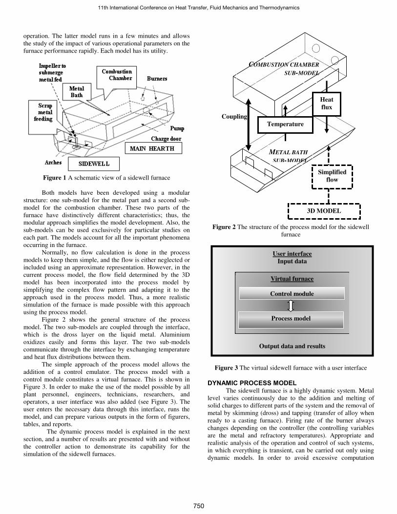
Figure 2 shows the general structure of the process

model. The two sub-models are coupled through the interface,

which is the dross layer on the liquid metal. Aluminium

oxidizes easily and forms this layer. The two sub-models

communicate through the interface by exchanging temperature

and heat flux distributions between them.

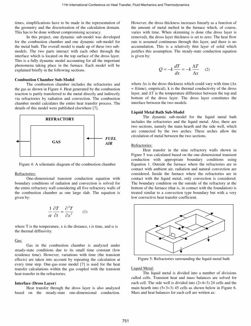
The simple approach of the process model allows the

addition of a control emulator. The process model with a

control module constitutes a virtual furnace. This is shown in

Figure 3. In order to make the use of the model possible by all

plant personnel, engineers, technicians, researchers, and

operators, a user interface was also added (see Figure 3). The

user enters the necessary data through this interface, runs the

model, and can prepare various outputs in the form of figurers,

tables, and reports.

The dynamic process model is explained in the next

section, and a number of results are presented with and without

the controller action to demonstrate its capability for the

simulation of the sidewell furnaces.

Figure 2 The structure of the process model for the sidewell

furnace

Figure 3 The virtual sidewell furnace with a user interface

DYNAMIC PROCESS MODEL The sidewell furnace is a highly dynamic system. Metal

level varies continuously due to the addition and melting of

solid charges to different parts of the system and the removal of

metal by skimming (dross) and tapping (transfer of alloy when

ready to a casting furnace). Firing rate of the burner always

changes depending on the controller (the controlling variables

are the metal and refractory temperatures). Appropriate and

realistic analysis of the operation and control of such systems,

in which everything is transient, can be carried out only using

dynamic models. In order to avoid excessive computation

User interface

Input data

Output data and results

Virtual furnace

Process model

Control module

COMBUSTION CHAMBER

SUB-MODEL

METAL BATH

SUB-MODEL

Coupling

Temperature

Heat

flux

3D MODEL

Simplified

flow


750

times, simplifications have to be made in the representation of

the geometry and the discretization of the calculation domain.

This has to be done without compromising accuracy.

In this project, one dynamic sub-model was developed

for the combustion chamber and one dynamic sub-model for

the metal bath. The overall model is made up of these two sub-

models. The two parts interact with each other through the

interface which is located on the top surface of the dross layer.

This is a fully dynamic model accounting for all the important

phenomena taking place in the furnace. Each model will be

explained briefly in the following sections.

Combustion Chamber Sub-Model The combustion chamber includes the refractories and

the gas as shown in Figure 4. Heat generated by the combustion

reaction is partly transferred to the metal directly and indirectly

via refractories by radiation and convection. The combustion

chamber model calculates the entire heat transfer process. The

details of this model were published elsewhere [7].

Figure 4: A schematic diagram of the combustion chamber

Refractories:

One-dimensional transient conduction equation with

boundary conditions of radiation and convection is solved for

the entire refractory wall considering all five refractory walls of

the combustion chamber as one large slab. The equation is

given by:

2

21

x

T

t

T

(1)

where T is the temperature, x is the distance, t is time, and is

the thermal diffusivity.

Gas:

Gas in the combustion chamber is analyzed under

steady-state conditions due to its small time constant (low

residence time). However, variations with time (the transient

effects) are taken into account by repeating the calculation at

every time step. One-gas-zone model [7] is used for the heat

transfer calculations within the gas coupled with the transient

heat transfer in the refractories.

Interface (Dross Layer)

Heat transfer through the dross layer is also analyzed

based on the steady-state one-dimensional conduction.

However, the dross thickness increases linearly as a function of

the amount of metal melted in the furnace which, of course,

varies with time. When skimming is done (the dross layer is

removed), the dross layer thickness is set to zero. The heat flow

rate is assumed continuous through this layer, and there is no

accumulation. This is a relatively thin layer of solid which

justifies this assumption. The steady-state conduction equation

is given by:

x

Tk

dx

dTkQ

(2)

where Δx is the dross thickness which could vary with time (Δx = f(time), empirical), k is the thermal conductivity of the dross

layer, and ΔT is the temperature difference between the top and bottom of the dross layer. The dross layer constitutes the

interface between the two models.

Liquid Metal Bath Sub-Model

The dynamic sub-model for the liquid metal bath

includes the refractories and the liquid metal. Also, there are

two sections, namely the main hearth and the side well, which

are connected by the two arches. These arches allow the

circulation of metal between the two sections.

Refractories:

Heat transfer in the nine refractory walls shown in

Figure 5 was calculated based on the one-dimensional transient

conduction with appropriate boundary conditions using

Equation 1. Outside the furnace where the refractories are in

contact with ambient air, radiation and natural convection are

considered. Inside the furnace where the refractories are in

contact with the liquid metal, only convection is considered.

The boundary condition on the outside of the refractory at the

bottom of the furnace (that is, in contact with the foundation) is

treated similar to a convection type boundary but with a very

low convective heat transfer coefficient.

Figure 5: Refractories surrounding the liquid metal bath

Liquid Metal:

The liquid metal is divided into a number of divisions

called cells. Transient heat and mass balances are solved for

each cell. The side well is divided into (243) 24 cells and the

main hearth into (533) 45 cells as shown below in Figure 6.

Mass and heat balances for each cell are written as:

GAS

REFRACTORY

FUEL

AIR


751

t

Vmm

t

moutin

)(

(3)

outinconduction QQQCpTVt

)( (4)

where V is the metal volume, V=f(h), h: liquid level which

varies with time; Qin is the heat input from all sources (such as

from the combustion chamber and due to flow into the cell,

depending on the location of the cell); Qout is the heat leaving

the cell (such as from heat loss to environment, due to flow out

of the cell, and melting of various charges, again depending on

the location of the cell); m is the mass flowrate entering or

leaving the cell; and Cp are the density and the specific heat

of the liquid metal.

Figure 6: Division of the side well and main hearth into cells

for dynamic heat and mass balance calculations

The detailed metal flow field was calculated for a

number of configurations of the system using the 3D model. A

simplified flow field was obtained through the above cells for

each configuration by simplifying the detailed flow profiles

carried out using the three-dimensional flow model. Depending

on the configuration used, the appropriate simplified flow field

is considered in the process model.

Solution procedure

The above equations were discretized. The relationships

between various geometric factors such as the variation of

furnace height as a function of furnace geometry were derived.

A control strategy was formulated.

At each time step, the events occurring at that time are

activated, the control emulator revises the controller output (the

necessary actions), then the two sub-models carry out the

calculations by exchanging temperatures and heat fluxes at the

interface. This is repeated at each time step until the end of the

furnace operation. The sidewell furnace simulator runs on PC.

The computation time is less than a minute for the simulation of

a 5-hour furnace operation.

The model calculates the temperature distribution in the

liquid metal and all refractories, the gas temperature in the

combustion chamber, the energy efficiency of the furnace, the

variation in the metal level, the amount of metal melted, etc., all

as a function of time for the entire operation.

Model validation The dynamic process model was validated by comparing

the model predictions with the plant data which were obtained

by carrying out a number of measurement campaigns in the

plant. A number of different cases were considered for

comparison. One case is given below.

For the validation work, the control emulator in the

model was deactivated. The shred flow rate and the fuel flow

rate were taken directly from the plant data. Consequently, the

control action on the furnace was implicitly included in the

model. Initial values of a number of parameters such as the

metal level were taken from the plant data as well. Initial

conditions in the furnace are crucial for the success of the

simulation. The plant data were studied in detail in an effort to

understand the conditions in the furnace at the beginning of the

test. Some of the discrepancies between the model predictions

and the plant data may be due to difficulty in specifying the

initial conditions.

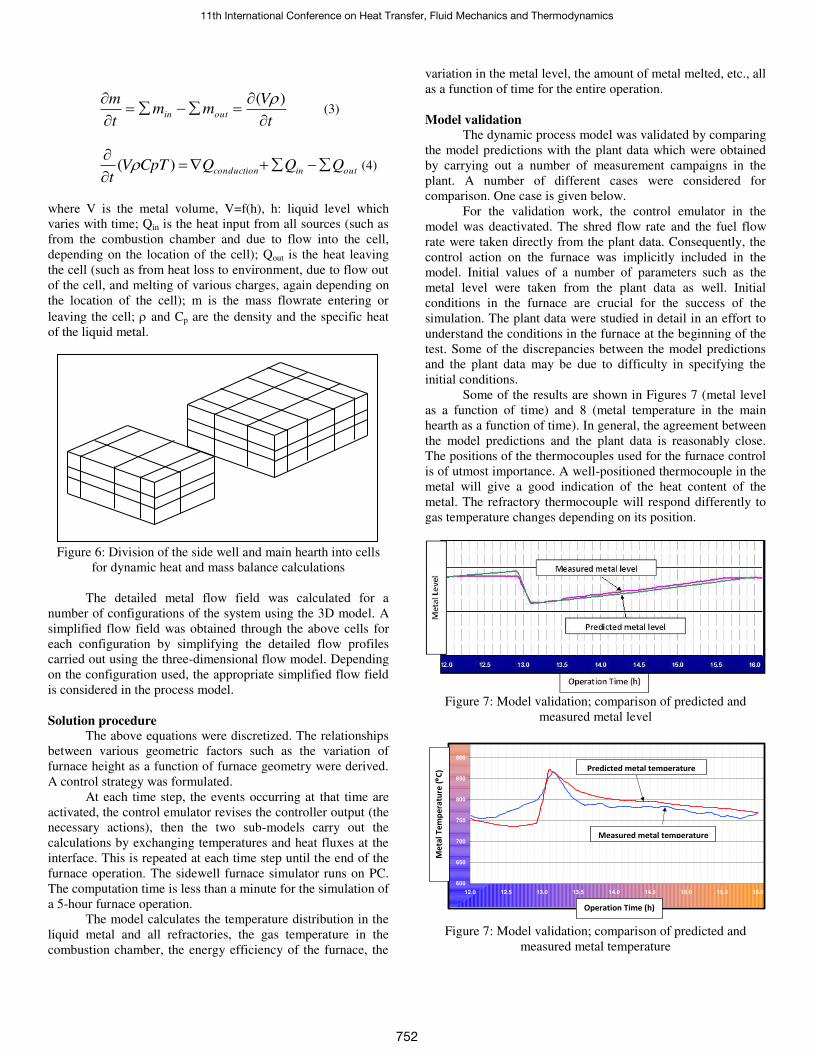
Some of the results are shown in Figures 7 (metal level

as a function of time) and 8 (metal temperature in the main

hearth as a function of time). In general, the agreement between

the model predictions and the plant data is reasonably close.

The positions of the thermocouples used for the furnace control

is of utmost importance. A well-positioned thermocouple in the

metal will give a good indication of the heat content of the

metal. The refractory thermocouple will respond differently to

gas temperature changes depending on its position.

Figure 7: Model validation; comparison of predicted and

measured metal level

Figure 7: Model validation; comparison of predicted and

measured metal temperature

600

650

700

750

800

850

900

12.0 12.5 13.0 13.5 14.0 14.5 15.0 15.5 16.0

Time (hours)

Ma

in H

ea

rth

Te

mp

era

ture

(C

)

measured

(thermocouple)

calculated by model

(thermocouple)

Operation Time (h)

Me

tal

Te

mp

era

ture

(C)

Measured metal temperature

Predicted metal temperature


752

RESULTS AND DISCUSSION The model was used to carry out parametric studies with

and without the controller action. Two examples are given below for each case.

A case study without the controller

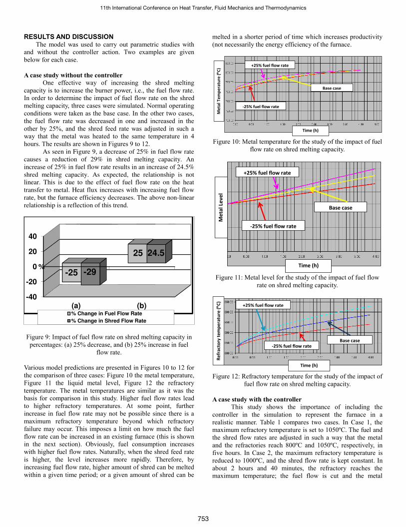
One effective way of increasing the shred melting capacity is to increase the burner power, i.e., the fuel flow rate. In order to determine the impact of fuel flow rate on the shred melting capacity, three cases were simulated. Normal operating conditions were taken as the base case. In the other two cases, the fuel flow rate was decreased in one and increased in the other by 25%, and the shred feed rate was adjusted in such a way that the metal was heated to the same temperature in 4 hours. The results are shown in Figures 9 to 12. As seen in Figure 9, a decrease of 25% in fuel flow rate

causes a reduction of 29% in shred melting capacity. An

increase of 25% in fuel flow rate results in an increase of 24.5%

shred melting capacity. As expected, the relationship is not

linear. This is due to the effect of fuel flow rate on the heat

transfer to metal. Heat flux increases with increasing fuel flow

rate, but the furnace efficiency decreases. The above non-linear

relationship is a reflection of this trend.

Figure 9: Impact of fuel flow rate on shred melting capacity in percentages: (a) 25% decrease, and (b) 25% increase in fuel

flow rate.

Various model predictions are presented in Figures 10 to 12 for the comparison of three cases: Figure 10 the metal temperature, Figure 11 the liquid metal level, Figure 12 the refractory temperature. The metal temperatures are similar as it was the basis for comparison in this study. Higher fuel flow rates lead to higher refractory temperatures. At some point, further increase in fuel flow rate may not be possible since there is a maximum refractory temperature beyond which refractory failure may occur. This imposes a limit on how much the fuel flow rate can be increased in an existing furnace (this is shown in the next section). Obviously, fuel consumption increases with higher fuel flow rates. Naturally, when the shred feed rate is higher, the level increases more rapidly. Therefore, by increasing fuel flow rate, higher amount of shred can be melted within a given time period; or a given amount of shred can be

melted in a shorter period of time which increases productivity (not necessarily the energy efficiency of the furnace.

Figure 10: Metal temperature for the study of the impact of fuel

flow rate on shred melting capacity.

Figure 11: Metal level for the study of the impact of fuel flow

rate on shred melting capacity.

Figure 12: Refractory temperature for the study of the impact of

fuel flow rate on shred melting capacity.

A case study with the controller

This study shows the importance of including the controller in the simulation to represent the furnace in a realistic manner. Table 1 compares two cases. In Case 1, the maximum refractory temperature is set to 1050ºC. The fuel and the shred flow rates are adjusted in such a way that the metal and the refractories reach 800ºC and 1050ºC, respectively, in five hours. In Case 2, the maximum refractory temperature is reduced to 1000ºC, and the shred flow rate is kept constant. In about 2 hours and 40 minutes, the refractory reaches the maximum temperature; the fuel flow is cut and the metal

-40

-20

0

20

40

(a) (b)

-25

25

-29

24.5

%

% Change in Fuel Flow Rate

% Change in Shred Flow Rate

Time (h)

Me

tal

Te

mp

era

ture

(C)

Base case

+25% fuel flow rate

-25% fuel flow rate

Time (h)

Me

tal

Lev

el

Base case

+25% fuel flow rate

-25% fuel flow rate

Time (h)

Re

fra

cto

ry t

em

pe

ratu

re (C)

Base case

+25% fuel flow rate

-25% fuel flow rate


753

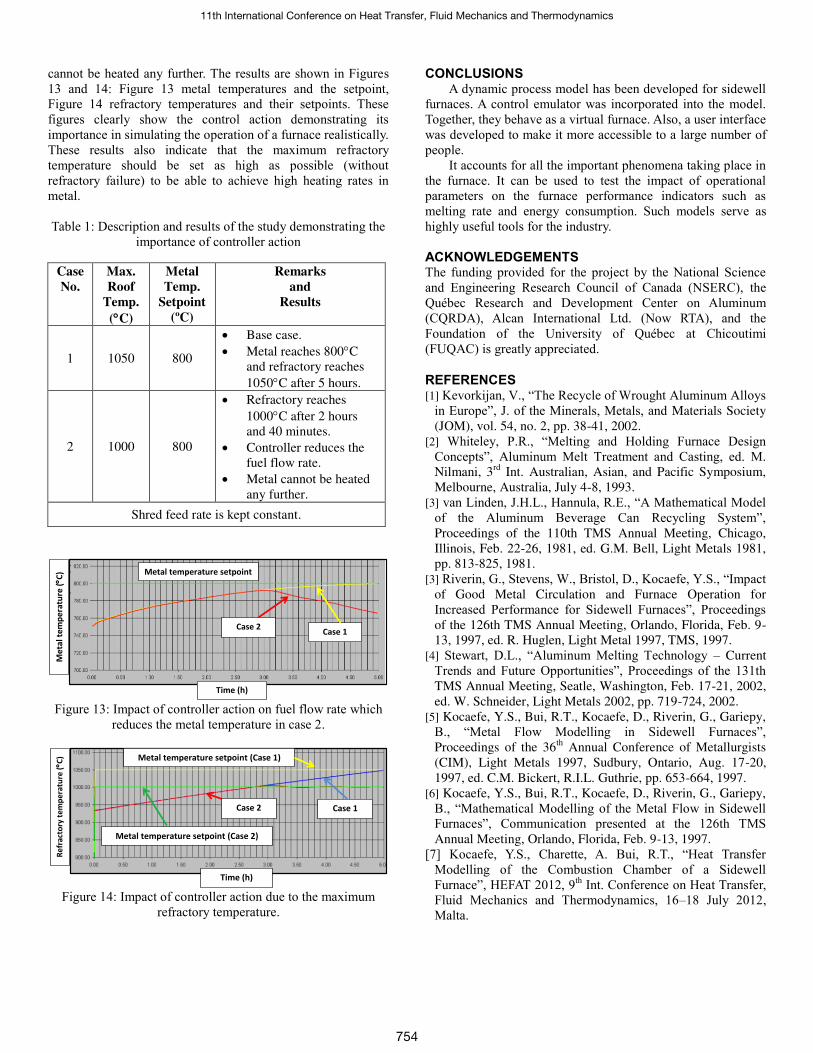
cannot be heated any further. The results are shown in Figures 13 and 14: Figure 13 metal temperatures and the setpoint, Figure 14 refractory temperatures and their setpoints. These figures clearly show the control action demonstrating its importance in simulating the operation of a furnace realistically. These results also indicate that the maximum refractory temperature should be set as high as possible (without refractory failure) to be able to achieve high heating rates in metal.

Table 1: Description and results of the study demonstrating the importance of controller action

Figure 13: Impact of controller action on fuel flow rate which

reduces the metal temperature in case 2.

Figure 14: Impact of controller action due to the maximum

refractory temperature.

CONCLUSIONS A dynamic process model has been developed for sidewell

furnaces. A control emulator was incorporated into the model. Together, they behave as a virtual furnace. Also, a user interface was developed to make it more accessible to a large number of people.

It accounts for all the important phenomena taking place in the furnace. It can be used to test the impact of operational parameters on the furnace performance indicators such as melting rate and energy consumption. Such models serve as highly useful tools for the industry.

ACKNOWLEDGEMENTS The funding provided for the project by the National Science and Engineering Research Council of Canada (NSERC), the Québec Research and Development Center on Aluminum (CQRDA), Alcan International Ltd. (Now RTA), and the Foundation of the University of Québec at Chicoutimi (FUQAC) is greatly appreciated.

REFERENCES [1] Kevorkijan, V., “The Recycle of Wrought Aluminum Alloys

in Europe”, J. of the Minerals, Metals, and Materials Society

(JOM), vol. 54, no. 2, pp. 38-41, 2002.

[2] Whiteley, P.R., “Melting and Holding Furnace Design Concepts”, Aluminum Melt Treatment and Casting, ed. M. Nilmani, 3

rd Int. Australian, Asian, and Pacific Symposium,

Melbourne, Australia, July 4-8, 1993.

[3] van Linden, J.H.L., Hannula, R.E., “A Mathematical Model of the Aluminum Beverage Can Recycling System”, Proceedings of the 110th TMS Annual Meeting, Chicago,

Illinois, Feb. 22-26, 1981, ed. G.M. Bell, Light Metals 1981,

pp. 813-825, 1981.

[3] Riverin, G., Stevens, W., Bristol, D., Kocaefe, Y.S., “Impact of Good Metal Circulation and Furnace Operation for

Increased Performance for Sidewell Furnaces”, Proceedings of the 126th TMS Annual Meeting, Orlando, Florida, Feb. 9-

13, 1997, ed. R. Huglen, Light Metal 1997, TMS, 1997.

[4] Stewart, D.L., “Aluminum Melting Technology – Current

Trends and Future Opportunities”, Proceedings of the 131th TMS Annual Meeting, Seatle, Washington, Feb. 17-21, 2002,

ed. W. Schneider, Light Metals 2002, pp. 719-724, 2002.

[5] Kocaefe, Y.S., Bui, R.T., Kocaefe, D., Riverin, G., Gariepy,

B., “Metal Flow Modelling in Sidewell Furnaces”, Proceedings of the 36

th Annual Conference of Metallurgists

(CIM), Light Metals 1997, Sudbury, Ontario, Aug. 17-20,

1997, ed. C.M. Bickert, R.I.L. Guthrie, pp. 653-664, 1997.

[6] Kocaefe, Y.S., Bui, R.T., Kocaefe, D., Riverin, G., Gariepy,

B., “Mathematical Modelling of the Metal Flow in Sidewell Furnaces”, Communication presented at the 126th TMS Annual Meeting, Orlando, Florida, Feb. 9-13, 1997.

[7] Kocaefe, Y.S., Charette, A. Bui, R.T., “Heat Transfer Modelling of the Combustion Chamber of a Sidewell Furnace”, HEFAT 2012, 9th Int. Conference on Heat Transfer, Fluid Mechanics and Thermodynamics, 16–18 July 2012, Malta.

Case 1

Me

tal

tem

pe

ratu

re (C)

Time (h)

Metal temperature setpoint

Case 2

Re

fra

cto

ry t

em

pe

ratu

re (C)

Case 1

Time (h)

Metal temperature setpoint (Case 1)

Case 2

Metal temperature setpoint (Case 2)

Case

No.

Max.

Roof

Temp.

(C)

Metal

Temp.

Setpoint

(ºC)

Remarks

and

Results

1 1050 800

Base case. Metal reaches 800C

and refractory reaches

1050C after 5 hours.

2 1000 800

Refractory reaches

1000C after 2 hours

and 40 minutes. Controller reduces the

fuel flow rate. Metal cannot be heated

any further.

Shred feed rate is kept constant.


754

SOLUTION OF RADIATIVE HEAT TRANSFER PROBLEMS USING THE SPHERICAL HARMONICS DISCRETE ORDINATES METHOD

Granate P.1, Coelho P.J.1* and Roger M.2 *Author for correspondence

1LAETA, IDMEC, Dept. of Mechanical Engineering, Instituto Superior Técnico, Universidade de Lisboa, Av. Rovisco Pais, 1049-001 Lisboa, Portugal

2Université de Lyon, INSA de Lyon, CETHIL, UMR5008, F-69621 Villeurbanne Cedex, France E-mail: [email protected]

ABSTRACT In this paper, a method that combines features of the

discrete ordinates and spherical harmonics method is presented. The method is based on the spherical harmonics discrete ordinates method, which was developed in the atmospheric radiation community, but the present implementation only retains some features of the original one. The method may be summarized in four steps. First, the source term of the RTE, which is evaluated in the spherical harmonics space, is converted to discrete ordinates. Second, the radiative transfer equation is solved using discrete ordinates. In this step, the standard discrete ordinates method is used, except in the evaluation of the source term. In the third step, the radiation intensity field in discrete ordinates space is transformed to spherical harmonics. Fourth, the source term of the RTE is calculated in the spherical harmonics space. The method is applied in the present work to solve radiative heat transfer problems in emitting, absorbing and scattering grey media. The predictions are assessed by means of comparison with benchmark solutions reported in the literature. It is shown that the proposed method has some advantages over the pure discrete ordinates and spherical harmonics methods, regarding both the accuracy and the computational time.

INTRODUCTION Many different methods have been developed over the years

to solve the radiative transfer equation (RTE) for participating media. Among them, the discrete ordinates method [1], DOM, is one of the most popular ones, due to the good balance of simplicity, accuracy, and computational economy. However, it is well known that it also suffers from several drawbacks, particularly the numerical smearing and the ray effects. A recent review of advances in this method is available [2]. The spherical harmonics method [3], SHM, has also been widely employed, namely the lowest order approximation, known as P1 approximation. This approximation often yields poor results, particularly if the medium is not optically thick, and the radiation field is far from isotropic. Higher order approximations are possible, but at the expense of additional complexity and computational requirements [4].

Modifications of the DOM aiming at an improvement of the accuracy have been proposed in the literature, e.g., the modified

DOM [5], the discrete ordinates interpolation method [6], the even parity formulation [7] and the method of lines [8]. Although these methods have a few advantages, at least for particular problems, the increased complexity of the formulation or the additional computational time limited their use.

Similarly, modifications of the SHM have been proposed, namely the modified differential approximation [9] and the improved differential approximation [10]. Despite the improvement achieved in some problems when using these modifications, they are unable to yield satisfactory results in many situations.

Another possibility is to combine somehow the P1 approximation and the DOM. A domain decomposition method in which the P1 method is used in optically thick regions and the RTE is solved elsewhere is described in [11]. A buffer zone between the two domains is used to couple the P1 and the RTE equations. The micro-macro model [12] decomposes the radiation intensity into a mesoscopic and a macroscopic equation, yielding a system of two coupled equations. The macroscopic component is the incident radiation, while the mesoscopic equation is mathematically similar to the RTE and may be solved using the DOM. A similar decomposition of the radiation intensity into two components is carried out in the hybrid transport-diffusion model [13]. However, the macroscopic component is no longer the incident radiation, but rather the solution of the P1 equation. In this model, the macroscopic equation is therefore the P1 equation, and may be efficiently solved using the classical numerical procedure. The mesoscopic equation is again mathematically similar to the RTE and the DOM can be used to solve it. In contrast to the micro-macro model, the macroscopic equation may be firstly solved, in a non-coupled way, and its solution is then used to solve the mesoscopic component. The methods reported in [11-13] are recent, and there is still limited assessment of their potential.

A different hybrid DOM-SHM is described in [14]. It relies on the decomposition of the radiation intensity into wall-emitted and medium radiation intensity components. This decomposition is similar to that used in the modified DOM and in the modified differential approximation. The wall-emitted radiation intensity component accounts for the extinction in the medium, due to absorption and out-scattering, of the radiation


755

emitted at the boundary, and it is calculated using the finite volume method, which is similar to the DOM. The medium radiation intensity component takes into account the radiation emitted in the medium and the in-scattering contribution. The P1 approximation is used for the medium-emitted part of the radiation intensity.

In the present work, a rather different hybrid method is employed. The original method was developed in the atmospheric radiation community, where it is referred to as SHDOM (spherical harmonics discrete ordinates method) [15], and has never been applied to radiative heat transfer problems, to the best of our knowledge. The present implementation is somewhat different from the original one, as described in the next section, but we still refer to the method as SHDOM, since the basic algorithm is retained.

MATHEMATICAL FORMULATION The RTE for an emitting-absorbing-scattering grey medium

may be written as follows [16]:

( ) ( ) ( )

( ) ( ) Ω′′Φ′+

++−=∇

∫⋅

dI

III

s

b

sssr

rsrsrs

,,4

,,

4ππσ

κβ (1)

where ( )sr,I is the radiation intensity in direction s, r is the position vector, Ib is the blackbody radiation intensity, κ, β and σs are the absorption, extinction and scattering coefficients of the medium, respectively, and ( )ss ,′Φ is the scattering phase function. The boundary condition for a grey surface that emits and reflects diffusely is given by [16]:

( ) ( ) ( ) Ω′′′+= ⋅⋅∫ <′dIII wwbw snsrrsr

sn,,

0πρε (2)

where ( )sr ,wI and ( )sr ′,wI are the radiation intensities at boundary point rw that leave the boundary along s direction and arrive along s′ direction, respectively, Ibw is the blackbody radiation intensity at the temperature of the boundary surface, ε is the surface emissivity, ρ is the surface reflectivity, and n is the unit vector normal to the surface and pointing into the medium.

In the present work, the spatial discretization of Eq. (1) is carried out using the finite volume method, as in the standard DOM. In contrast, in the original formulation of the SHDOM [15], the RTE is expressed in integral form, and integrated along the discrete directions, following a procedure similar to that used in the discrete ordinates interpolation method [6]. In addition, an adaptive grid is used in the original method. These features of the original SHDOM are not used in the present work, which relies on the standard DOM formulation regarding the spatial discretization. The radiation intensities at the cell faces were calculated using the CLAM scheme. The angular discretization of Eq. (1) was carried out using the SN quadrature, except for the in-scattering term, which is discussed

below. Details on the discretization procedure may be found elsewhere [17].

When the DOM is employed, all the angular integrals are approximated by a quadrature. In the SHDOM, however, the in-scattering term of the RTE is calculated using spherical harmonics, according to the original SHDOM formulation. Denoting the in-scattering term of the RTE by SSH(r,s), the following truncated expansion in spherical harmonics is taken:

( ) ( ) ( ) ( ) ( )rssssrsrSHml

L

l

M

Mm

ml

s SYdIS ∑ ∑∫= −=

=Ω′′Φ′=0

4,,

4,

ππσ

(3)

In this equation, ( )smlY are spherical harmonics, ( )rm

lS are coefficients that depend only on the spatial coordinates, and M ≤ L. Note that terms such that M > l are equal to zero. The real spherical harmonics are defined as follows:

( ) ( ) ( ) ( )( )( ) ( ) ( )φμ

δπφμ muP

mlmll

muY ml

mo

ml

ml !

!12

12−

−

++

=Λ=s

(4)

where mlΛ are associated Legendre functions, ( )μm

lP are associated Legendre polynomials, and u(mφ) = cos(mφ) if m≥0 and u(mφ) = sin(mφ) if m<0. The in-scattering term is transformed to discrete ordinates as follows:

( ) ( ) ( ) ( )rsrDOMml

L

l

M

Mmkj

mljk SmuS ∑ ∑

= −=

Λ=0

, φμ (5)

where μj=cosθj and subscripts j and k identify one among the Nd directions of the DOM angular discretization. The RTE is solved using the in-scattering term given by equation (5) to obtain the radiation intensity for every direction, namely Ijk(r)=I(r,sjk).

The radiation intensity at every grid node, evaluated from the DOM, is transformed to spherical harmonics space as follows:

( ) ( ) ( )rssrSHml

ml

L

l

M

MmIYI ∑ ∑

= −=

=0

, (6)

The coefficients ( )rm

lI are given by

( ) ( ) ( ) ( ) ( ) ( )

( ) ( ) ( )jkkjmlk

N

j

N

kj

ml

ml

ml

Imu

dImudIYI

sr

srsrsr

,

,,

1 1

44

φμωω

φμ

μ φ

ππ

Λ=

ΩΛ=Ω=

∑ ∑

∫∫

= =

(7) where Nμ and Nφ are the number of cosine polar angles and the


756

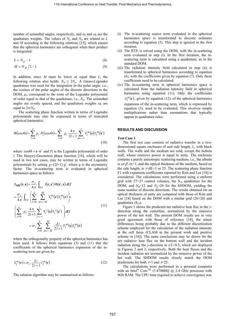
number of azimuthal angles, respectively, and ωj and ωk are the quadrature weights. The values of Nμ and Nφ are related to L and M according to the following relations [15], which ensure that the spherical harmonics are orthogonal when their product is integrated:

1−= μNL (8)

12 −= φNM (9) In addition, since M must be lower or equal than L, the following relation also holds: Nφ ≤ 2Nμ. A Gauss-Legendre quadrature was used for the integration in the polar angle, i.e., the cosines of the polar angles of the discrete directions in the DOM, μj, correspond to the roots of the Legendre polynomial of order equal to that of the quadrature, i.e., Nμ. The azimuthal angles are evenly spaced, and the quadrature weights ωk are equal to 2π/Nφ.

The scattering phase function written in terms of Legendre polynomials may also be expressed in terms of truncated spherical harmonics:

( ) ( ) ( ) ( )ss ′+

=Θ=ΘΦ ∑∑∑−===

ml

l

lm

ml

L

ll

L

lll YY

lP

00 124coscos π

χχ

(10) where ss ′⋅=Θcos and Pl is the Legendre polynomial of order l. The Henyey-Greenstein phase function [16], which will be used in two test cases, may be written in terms of Legendre polynomials by setting χl=(2l+1) gl, where g is the asymmetry factor. The in-scattering term is evaluated in spherical harmonics space as follows:

( ) ( ) ( )

( ) ( )

( ) ( )

( ) ( )rs

ss

rs

sssrsrSH

ml

ml

lL

l

M

Mms

ji

L

i

i

ij

jii

ml

ml

L

l

M

Mm

s

s

IYl

dYYi

IY

dIS

12

124

'4

,,4

,

0

0

40

4

+=

Ω′⎟⎟⎟

⎠

⎞

⎜⎜⎜

⎝

⎛′

+

×⎟⎟

⎠

⎞

⎜⎜

⎝

⎛=

Ω′′Φ′=

∑ ∑

∑ ∑

∫ ∑ ∑

∫

= −=

= −=

= −=

χσ

πχ

πσ

πσ

π

π

(11)

where the orthogonality property of the spherical harmonics has been used. It follows from equations (3) and (11) that the coefficients of the spherical harmonics expansion of the in-scattering term are given by:

( ) ( )rr ml

ls

ml I

lS

12 +=

χσ (12)

The solution algorithm may be summarized as follows:

(i) The in-scattering source term evaluated in the spherical harmonics space is transformed to discrete ordinates according to equation (5). This step is ignored in the first iteration.

(ii) The RTE is solved using the DOM, with the in-scattering term evaluated in step (i). In the first iteration, the in-scattering term is calculated using a quadrature, as in the standard DOM.

(iii) The radiation intensity field calculated in step (ii) is transformed to spherical harmonics according to equation (6), with the coefficients given by equation (7). Only these coefficients need to be calculated.

(iv) The in-scattering term in spherical harmonics space is calculated from the radiation intensity field in spherical harmonics using equation (11). Only the coefficients

( )rmlS , given by equation (12), of the spherical harmonics

expansion of the in-scattering term, which is expressed by equation (3), need to be evaluated. This involves simple multiplications rather than summations that typically appear in quadrature rules.

RESULTS AND DISCUSSION Test Case 1

The first test case consists of radiative transfer in a two-dimensional square enclosure of unit side length, L, with black walls. The walls and the medium are cold, except the bottom wall, whose emissive power is equal to unity. The enclosure contains a purely anisotropic scattering medium, i.e., the albedo is ω=β /σs=1, and the optical thickness of the medium, based on the side length, is τ=βL=1 or 25. The scattering phase function F1 with expansion coefficients reported by Kim and Lee [18] is considered. The calculations were performed using a uniform grid with 27×27 control volumes, the S16 quadrature for the DOM, and Nφ=12 and Nμ=24 for the SHDOM, yielding the same number of discrete directions. The results obtained for an optical thickness of unity are compared with those of Kim and Lee [18] based on the DOM with a similar grid (26×26) and quadrature (S14).

Figure 1 shows the predicted net radiative heat flux in the y-direction along the centerline, normalized by the emissive power of the hot wall. The present DOM results are in very good agreement with those of reference [18], the minor differences being probably due to the different discretization scheme employed for the calculation of the radiation intensity at the cell faces (CLAM in the present work and positive scheme in [18]). The same conclusions may be drawn for the net radiative heat flux on the bottom wall and the incident radiation along the y-direction at x/L=0.5, which are displayed in Figures 2 and 3, respectively. Both the heat fluxes and the incident radiation are normalized by the emissive power of the hot wall. The SHDOM results closely match the DOM predictions for both τ=1 and τ=25.

The calculations were performed in a personal computer with an Intel® CoreTM i7-4700HQ @ 2.4 GHz processor with 8Gb RAM. The CPU time required to achieve convergence was


757

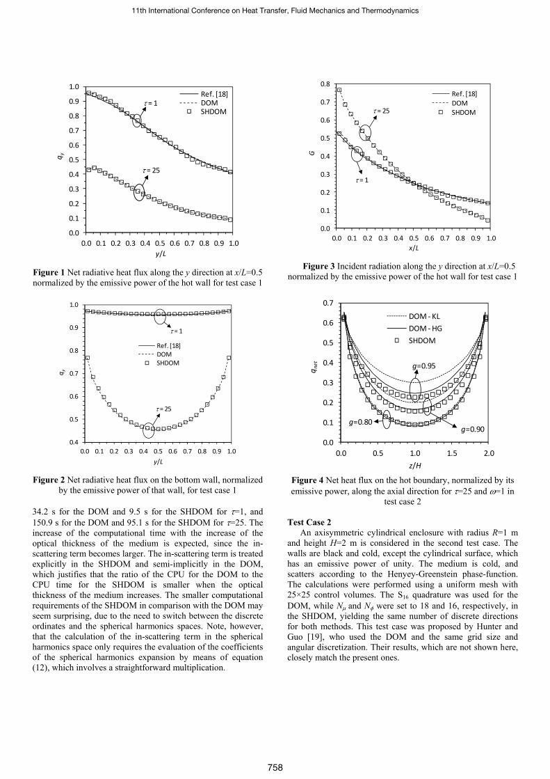
0.0

0.1

0.2

0.3

0.4

0.5

0.6

0.7

0.8

0.9

1.0

0.0 0.1 0.2 0.3 0.4 0.5 0.6 0.7 0.8 0.9 1.0

q y

y/L

Ref. [18]DOMSHDOM

τ = 1

τ = 25

Figure 1 Net radiative heat flux along the y direction at x/L=0.5 normalized by the emissive power of the hot wall for test case 1

0.4

0.5

0.6

0.7

0.8

0.9

1.0

0.0 0.1 0.2 0.3 0.4 0.5 0.6 0.7 0.8 0.9 1.0

q y

y/L

Ref. [18]DOMSHDOM

τ = 1

τ = 25

Figure 2 Net radiative heat flux on the bottom wall, normalized

by the emissive power of that wall, for test case 1 34.2 s for the DOM and 9.5 s for the SHDOM for τ=1, and 150.9 s for the DOM and 95.1 s for the SHDOM for τ=25. The increase of the computational time with the increase of the optical thickness of the medium is expected, since the in-scattering term becomes larger. The in-scattering term is treated explicitly in the SHDOM and semi-implicitly in the DOM, which justifies that the ratio of the CPU for the DOM to the CPU time for the SHDOM is smaller when the optical thickness of the medium increases. The smaller computational requirements of the SHDOM in comparison with the DOM may seem surprising, due to the need to switch between the discrete ordinates and the spherical harmonics spaces. Note, however, that the calculation of the in-scattering term in the spherical harmonics space only requires the evaluation of the coefficients of the spherical harmonics expansion by means of equation (12), which involves a straightforward multiplication.

0.0

0.1

0.2

0.3

0.4

0.5

0.6

0.7

0.8

0.0 0.1 0.2 0.3 0.4 0.5 0.6 0.7 0.8 0.9 1.0

G

x/L

Ref. [18]DOMSHDOMτ = 25

τ = 1

Figure 3 Incident radiation along the y direction at x/L=0.5

normalized by the emissive power of the hot wall for test case 1

0.0

0.1

0.2

0.3

0.4

0.5

0.6

0.7

0.0 0.5 1.0 1.5 2.0

q net

z/H

DOM ‐ KLDOM ‐HGSHDOM

g=0.95

g=0.90g=0.80

Figure 4 Net heat flux on the hot boundary, normalized by its emissive power, along the axial direction for τ=25 and ω=1 in

test case 2 Test Case 2

An axisymmetric cylindrical enclosure with radius R=1 m and height H=2 m is considered in the second test case. The walls are black and cold, except the cylindrical surface, which has an emissive power of unity. The medium is cold, and scatters according to the Henyey-Greenstein phase-function. The calculations were performed using a uniform mesh with 25×25 control volumes. The S16 quadrature was used for the DOM, while Nμ and Nφ were set to 18 and 16, respectively, in the SHDOM, yielding the same number of discrete directions for both methods. This test case was proposed by Hunter and Guo [19], who used the DOM and the same grid size and angular discretization. Their results, which are not shown here, closely match the present ones.


758

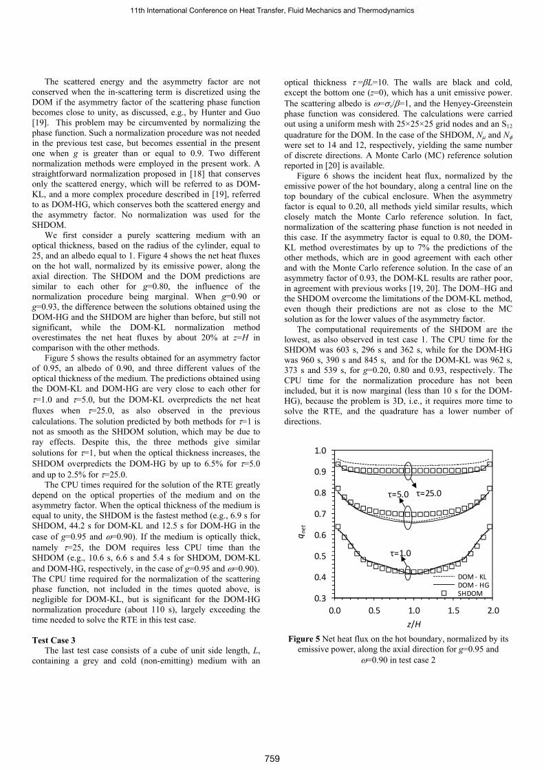
The scattered energy and the asymmetry factor are not conserved when the in-scattering term is discretized using the DOM if the asymmetry factor of the scattering phase function becomes close to unity, as discussed, e.g., by Hunter and Guo [19]. This problem may be circumvented by normalizing the phase function. Such a normalization procedure was not needed in the previous test case, but becomes essential in the present one when g is greater than or equal to 0.9. Two different normalization methods were employed in the present work. A straightforward normalization proposed in [18] that conserves only the scattered energy, which will be referred to as DOM-KL, and a more complex procedure described in [19], referred to as DOM-HG, which conserves both the scattered energy and the asymmetry factor. No normalization was used for the SHDOM.

We first consider a purely scattering medium with an optical thickness, based on the radius of the cylinder, equal to 25, and an albedo equal to 1. Figure 4 shows the net heat fluxes on the hot wall, normalized by its emissive power, along the axial direction. The SHDOM and the DOM predictions are similar to each other for g=0.80, the influence of the normalization procedure being marginal. When g=0.90 or g=0.93, the difference between the solutions obtained using the DOM-HG and the SHDOM are higher than before, but still not significant, while the DOM-KL normalization method overestimates the net heat fluxes by about 20% at z=H in comparison with the other methods.

Figure 5 shows the results obtained for an asymmetry factor of 0.95, an albedo of 0.90, and three different values of the optical thickness of the medium. The predictions obtained using the DOM-KL and DOM-HG are very close to each other for τ=1.0 and τ=5.0, but the DOM-KL overpredicts the net heat fluxes when τ=25.0, as also observed in the previous calculations. The solution predicted by both methods for τ=1 is not as smooth as the SHDOM solution, which may be due to ray effects. Despite this, the three methods give similar solutions for τ=1, but when the optical thickness increases, the SHDOM overpredicts the DOM-HG by up to 6.5% for τ=5.0 and up to 2.5% for τ=25.0.

The CPU times required for the solution of the RTE greatly depend on the optical properties of the medium and on the asymmetry factor. When the optical thickness of the medium is equal to unity, the SHDOM is the fastest method (e.g., 6.9 s for SHDOM, 44.2 s for DOM-KL and 12.5 s for DOM-HG in the case of g=0.95 and ω=0.90). If the medium is optically thick, namely τ=25, the DOM requires less CPU time than the SHDOM (e.g., 10.6 s, 6.6 s and 5.4 s for SHDOM, DOM-KL and DOM-HG, respectively, in the case of g=0.95 and ω=0.90). The CPU time required for the normalization of the scattering phase function, not included in the times quoted above, is negligible for DOM-KL, but is significant for the DOM-HG normalization procedure (about 110 s), largely exceeding the time needed to solve the RTE in this test case.

Test Case 3

The last test case consists of a cube of unit side length, L, containing a grey and cold (non-emitting) medium with an

optical thickness τ =βL=10. The walls are black and cold, except the bottom one (z=0), which has a unit emissive power. The scattering albedo is ω=σs/β=1, and the Henyey-Greenstein phase function was considered. The calculations were carried out using a uniform mesh with 25×25×25 grid nodes and an S12 quadrature for the DOM. In the case of the SHDOM, Nμ and Nφ were set to 14 and 12, respectively, yielding the same number of discrete directions. A Monte Carlo (MC) reference solution reported in [20] is available.

Figure 6 shows the incident heat flux, normalized by the emissive power of the hot boundary, along a central line on the top boundary of the cubical enclosure. When the asymmetry factor is equal to 0.20, all methods yield similar results, which closely match the Monte Carlo reference solution. In fact, normalization of the scattering phase function is not needed in this case. If the asymmetry factor is equal to 0.80, the DOM-KL method overestimates by up to 7% the predictions of the other methods, which are in good agreement with each other and with the Monte Carlo reference solution. In the case of an asymmetry factor of 0.93, the DOM-KL results are rather poor, in agreement with previous works [19, 20]. The DOM–HG and the SHDOM overcome the limitations of the DOM-KL method, even though their predictions are not as close to the MC solution as for the lower values of the asymmetry factor.

The computational requirements of the SHDOM are the lowest, as also observed in test case 1. The CPU time for the SHDOM was 603 s, 296 s and 362 s, while for the DOM-HG was 960 s, 390 s and 845 s, and for the DOM-KL was 962 s, 373 s and 539 s, for g=0.20, 0.80 and 0.93, respectively. The CPU time for the normalization procedure has not been included, but it is now marginal (less than 10 s for the DOM-HG), because the problem is 3D, i.e., it requires more time to solve the RTE, and the quadrature has a lower number of directions.

0.3

0.4

0.5

0.6

0.7

0.8

0.9

1.0

0.0 0.5 1.0 1.5 2.0

q net

z/H

DOM ‐ KLDOM ‐ HGSHDOM

τ=25.0

τ=1.0

τ=5.0

Figure 5 Net heat flux on the hot boundary, normalized by its

emissive power, along the axial direction for g=0.95 and ω=0.90 in test case 2


759

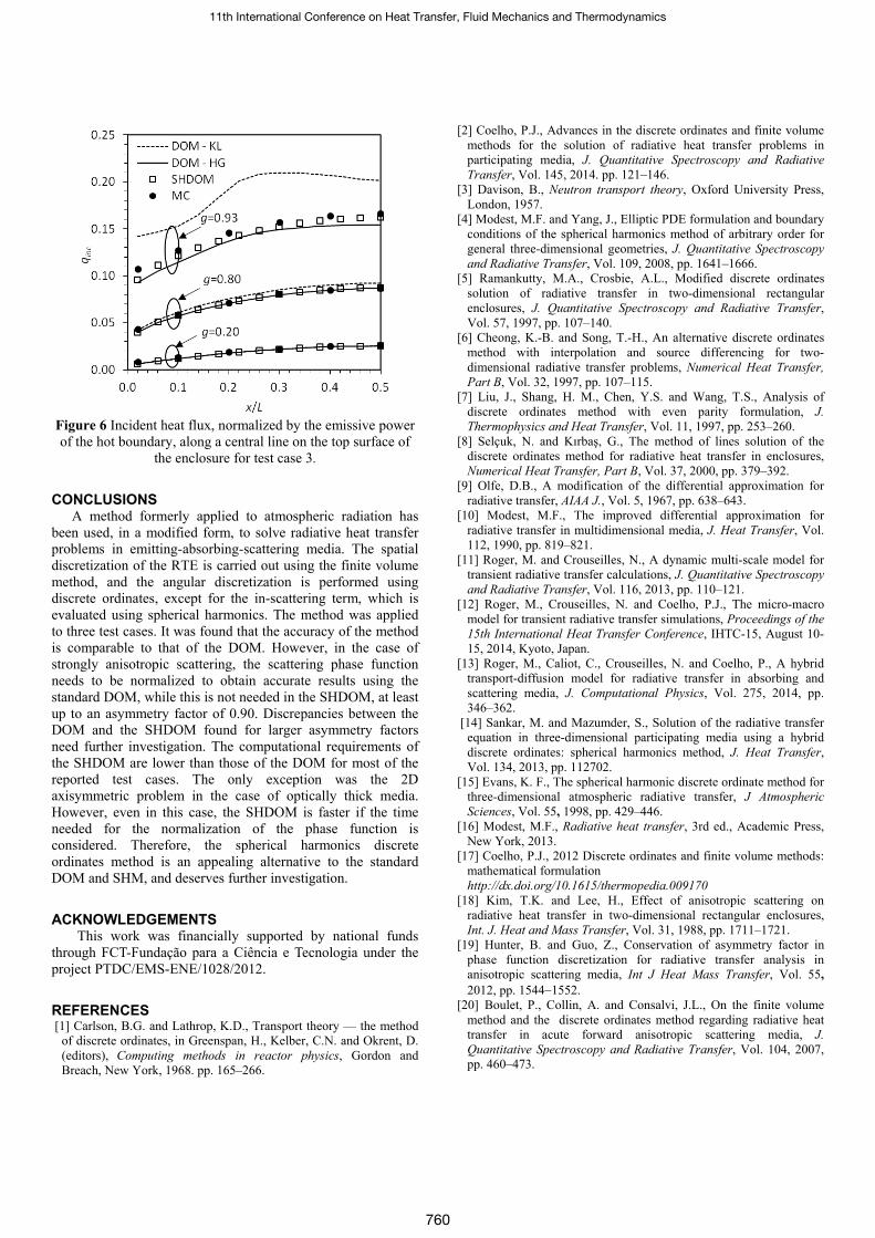
Figure 6 Incident heat flux, normalized by the emissive power of the hot boundary, along a central line on the top surface of

the enclosure for test case 3.

CONCLUSIONS A method formerly applied to atmospheric radiation has

been used, in a modified form, to solve radiative heat transfer problems in emitting-absorbing-scattering media. The spatial discretization of the RTE is carried out using the finite volume method, and the angular discretization is performed using discrete ordinates, except for the in-scattering term, which is evaluated using spherical harmonics. The method was applied to three test cases. It was found that the accuracy of the method is comparable to that of the DOM. However, in the case of strongly anisotropic scattering, the scattering phase function needs to be normalized to obtain accurate results using the standard DOM, while this is not needed in the SHDOM, at least up to an asymmetry factor of 0.90. Discrepancies between the DOM and the SHDOM found for larger asymmetry factors need further investigation. The computational requirements of the SHDOM are lower than those of the DOM for most of the reported test cases. The only exception was the 2D axisymmetric problem in the case of optically thick media. However, even in this case, the SHDOM is faster if the time needed for the normalization of the phase function is considered. Therefore, the spherical harmonics discrete ordinates method is an appealing alternative to the standard DOM and SHM, and deserves further investigation.

ACKNOWLEDGEMENTS This work was financially supported by national funds

through FCT-Fundação para a Ciência e Tecnologia under the project PTDC/EMS-ENE/1028/2012.

REFERENCES [1] Carlson, B.G. and Lathrop, K.D., Transport theory — the method

of discrete ordinates, in Greenspan, H., Kelber, C.N. and Okrent, D. (editors), Computing methods in reactor physics, Gordon and Breach, New York, 1968. pp. 165–266.

[2] Coelho, P.J., Advances in the discrete ordinates and finite volume methods for the solution of radiative heat transfer problems in participating media, J. Quantitative Spectroscopy and Radiative Transfer, Vol. 145, 2014. pp. 121–146.

[3] Davison, B., Neutron transport theory, Oxford University Press, London, 1957.

[4] Modest, M.F. and Yang, J., Elliptic PDE formulation and boundary conditions of the spherical harmonics method of arbitrary order for general three-dimensional geometries, J. Quantitative Spectroscopy and Radiative Transfer, Vol. 109, 2008, pp. 1641–1666.

[5] Ramankutty, M.A., Crosbie, A.L., Modified discrete ordinates solution of radiative transfer in two-dimensional rectangular enclosures, J. Quantitative Spectroscopy and Radiative Transfer, Vol. 57, 1997, pp. 107–140.

[6] Cheong, K.-B. and Song, T.-H., An alternative discrete ordinates method with interpolation and source differencing for two-dimensional radiative transfer problems, Numerical Heat Transfer, Part B, Vol. 32, 1997, pp. 107–115.

[7] Liu, J., Shang, H. M., Chen, Y.S. and Wang, T.S., Analysis of discrete ordinates method with even parity formulation, J. Thermophysics and Heat Transfer, Vol. 11, 1997, pp. 253–260.

[8] Selçuk, N. and Kırbaş, G., The method of lines solution of the discrete ordinates method for radiative heat transfer in enclosures, Numerical Heat Transfer, Part B, Vol. 37, 2000, pp. 379–392.

[9] Olfe, D.B., A modification of the differential approximation for radiative transfer, AIAA J., Vol. 5, 1967, pp. 638–643.

[10] Modest, M.F., The improved differential approximation for radiative transfer in multidimensional media, J. Heat Transfer, Vol. 112, 1990, pp. 819–821.

[11] Roger, M. and Crouseilles, N., A dynamic multi-scale model for transient radiative transfer calculations, J. Quantitative Spectroscopy and Radiative Transfer, Vol. 116, 2013, pp. 110–121.

[12] Roger, M., Crouseilles, N. and Coelho, P.J., The micro-macro model for transient radiative transfer simulations, Proceedings of the 15th International Heat Transfer Conference, IHTC-15, August 10-15, 2014, Kyoto, Japan.

[13] Roger, M., Caliot, C., Crouseilles, N. and Coelho, P., A hybrid transport-diffusion model for radiative transfer in absorbing and scattering media, J. Computational Physics, Vol. 275, 2014, pp. 346–362.

[14] Sankar, M. and Mazumder, S., Solution of the radiative transfer equation in three-dimensional participating media using a hybrid discrete ordinates: spherical harmonics method, J. Heat Transfer, Vol. 134, 2013, pp. 112702.

[15] Evans, K. F., The spherical harmonic discrete ordinate method for three-dimensional atmospheric radiative transfer, J Atmospheric Sciences, Vol. 55, 1998, pp. 429–446.

[16] Modest, M.F., Radiative heat transfer, 3rd ed., Academic Press, New York, 2013.

[17] Coelho, P.J., 2012 Discrete ordinates and finite volume methods: mathematical formulation http://dx.doi.org/10.1615/thermopedia.009170

[18] Kim, T.K. and Lee, H., Effect of anisotropic scattering on radiative heat transfer in two-dimensional rectangular enclosures, Int. J. Heat and Mass Transfer, Vol. 31, 1988, pp. 1711–1721.

[19] Hunter, B. and Guo, Z., Conservation of asymmetry factor in phase function discretization for radiative transfer analysis in anisotropic scattering media, Int J Heat Mass Transfer, Vol. 55, 2012, pp. 1544−1552.

[20] Boulet, P., Collin, A. and Consalvi, J.L., On the finite volume method and the discrete ordinates method regarding radiative heat transfer in acute forward anisotropic scattering media, J. Quantitative Spectroscopy and Radiative Transfer, Vol. 104, 2007, pp. 460–473.


760

NUMERICAL STUDY ON ENERGY CONSUMPTION CHARACTERISTICS FOR

DIFFERENT WALL STRUCTURES AND DIFFERENT THICKNESS OF THERMAL

INSULATION LAYER BASED ON THE INTERMITTENT ENERGY USE

CHARACTERISTICS

Bin Zhou

Department of Energy Engineering, Zhejiang University

38 Zheda Road, Hangzhou, 310027， PR China

Xiao-qian Qian

Department of Civil Engineering and Architecture, Zhejiang University

866 Yuhangtang Road, Hangzhou, 310058, PR China

David Kulkuka

Department of Mechanical Engineering Technology, State University of New York College

Buffalo, United States

Wei Li*

Department of Energy Engineering, Zhejiang University

38 Zheda Road, Hangzhou, 310027


Yu-Zhen Niu

Fortune Group Co Ltd，Hangzhou, 310000，P.R. China

ABSTRACT

Based on the intermittent energy use characteristics of a

hot summer and cold winter zone, a 3-D dynamic heat transfer

model is proposed to study the cooling requirements for a

typical household in Shanghai. A determination of the

influence of different wall structures (self-insulation structure,

non-insulated structure, exterior insulation structure, interior

insulation structure) on the energy consumption is made using

numerical calculations and analysis. Results show that the

interior insulation structure provides a reduction of energy

consumption, while the exterior insulation structure (the most

widely used insulation structure) does not exhibit an energy

saving effect. For the interior insulation structure, the thermal

insulation thickness of 0.03m is appropriate.

INTRODUCTION Building energy is the largest energy consumer in China’s,

using approximately 27.5% of the total energy consumption.

Over the next 20 years building energy consumption is

expected to rise to approximately 40% [1]. Efficient building

energy design involves a variety of technologies including:

energy-saving building envelope technology; heating and

cooling system design; and energy-saving construction

equipment technology (renewable energy applications in

buildings etc.). Currently, efficient building envelope energy

design is the dominant technology.

China’s is a vast territory with different regions having

distinct climate characteristics. A typical climate would be a

“hot-summer and cold winter” zone that is characterized by an

extremely hot summer with a wet and cold winter. The zone is

located around Shanghai in center-east part of China with

population of 300 million. Several previous studies [2] on

efficient building energy designs have been performed to

study methods of enhancement. Exterior insulation is currently

the primary structure used in northern heating areas, however

designs that consider this design typically ignores intermittent

energy use characteristics and when that type of usage is

considered its results are not ideal.

Florides [3] studied natural and artificial ventilation,

shading, glass type, shape and orientation of buildings, wall

insulation, roof insulation, etc. using the TRNSYS software.

They analyzed energy consumption and calculated the life

cycle cost for heating and cooling. Lindberg [4] carried out a 5

year study on a building with different exterior walls. Results


761

https://edas.info/showPerson.php?p=1200745&c=18877

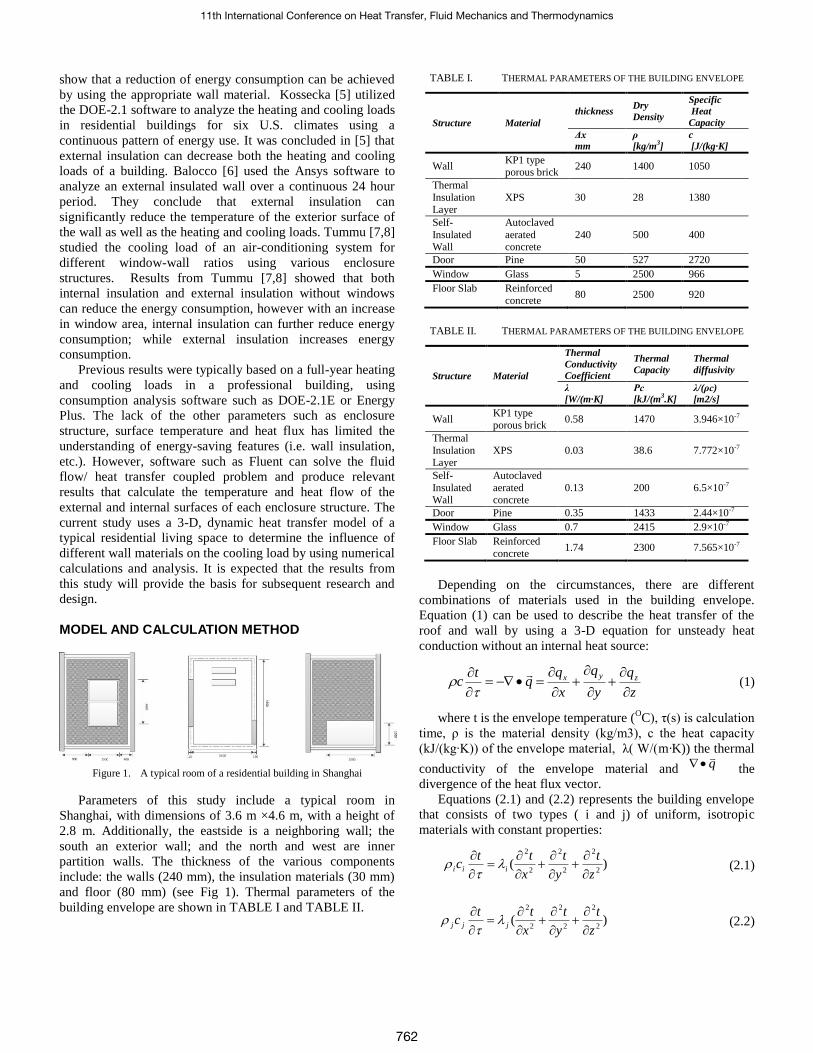
show that a reduction of energy consumption can be achieved

by using the appropriate wall material. Kossecka [5] utilized

the DOE-2.1 software to analyze the heating and cooling loads

in residential buildings for six U.S. climates using a

continuous pattern of energy use. It was concluded in [5] that

external insulation can decrease both the heating and cooling

loads of a building. Balocco [6] used the Ansys software to

analyze an external insulated wall over a continuous 24 hour

period. They conclude that external insulation can

significantly reduce the temperature of the exterior surface of

the wall as well as the heating and cooling loads. Tummu [7,8]

studied the cooling load of an air-conditioning system for

different window-wall ratios using various enclosure

structures. Results from Tummu [7,8] showed that both

internal insulation and external insulation without windows

can reduce the energy consumption, however with an increase

in window area, internal insulation can further reduce energy

consumption; while external insulation increases energy

consumption.

Previous results were typically based on a full-year heating

and cooling loads in a professional building, using

consumption analysis software such as DOE-2.1E or Energy

Plus. The lack of the other parameters such as enclosure

structure, surface temperature and heat flux has limited the

understanding of energy-saving features (i.e. wall insulation,

etc.). However, software such as Fluent can solve the fluid

flow/ heat transfer coupled problem and produce relevant

results that calculate the temperature and heat flow of the

external and internal surfaces of each enclosure structure. The

current study uses a 3-D, dynamic heat transfer model of a

typical residential living space to determine the influence of

different wall materials on the cooling load by using numerical

calculations and analysis. It is expected that the results from

this study will provide the basis for subsequent research and

design.

MODEL AND CALCULATION METHOD

Figure 1. A typical room of a residential building in Shanghai

Parameters of this study include a typical room in

Shanghai, with dimensions of 3.6 m ×4.6 m, with a height of

2.8 m. Additionally, the eastside is a neighboring wall; the

south an exterior wall; and the north and west are inner

partition walls. The thickness of the various components

include: the walls (240 mm), the insulation materials (30 mm)

and floor (80 mm) (see Fig 1). Thermal parameters of the

building envelope are shown in TABLE I and TABLE II.

TABLE I. THERMAL PARAMETERS OF THE BUILDING ENVELOPE

Structure Material

thickness Dry

Density

Specific

Heat

Capacity

Δx

mm

ρ

[kg/m3]

c

[J/(kg·K]

Wall KP1 type porous brick

240 1400 1050

Thermal

Insulation Layer

XPS 30 28 1380

Self-

Insulated Wall

Autoclaved

aerated concrete

240 500 400

Door Pine 50 527 2720

Window Glass 5 2500 966

Floor Slab

Reinforced

concrete 80 2500 920

TABLE II. THERMAL PARAMETERS OF THE BUILDING ENVELOPE

Structure Material

Thermal

Conductivity

Coefficient

Thermal

Capacity

Thermal

diffusivity

λ

[W/(m·K]

Ρc

[kJ/(m3.K]

λ/(ρc)

[m2/s]

Wall KP1 type porous brick

0.58 1470 3.946×10-7

Thermal

Insulation Layer

XPS 0.03 38.6 7.772×10-7

Self-

Insulated Wall

Autoclaved

aerated concrete

0.13 200 6.5×10-7

Door Pine 0.35 1433 2.44×10-7

Window Glass 0.7 2415 2.9×10-7

Floor Slab

Reinforced

concrete 1.74 2300 7.565×10-7

Depending on the circumstances, there are different

combinations of materials used in the building envelope.

Equation (1) can be used to describe the heat transfer of the

roof and wall by using a 3-D equation for unsteady heat

conduction without an internal heat source:

z

q

y

q

x

qq

tc zyx

(1)

where t is the envelope temperature (OC), τ(s) is calculation

time, ρ is the material density (kg/m3), c the heat capacity

(kJ/(kg·K)) of the envelope material, λ( W/(m·K)) the thermal

conductivity of the envelope material and q

the

divergence of the heat flux vector.

Equations (2.1) and (2.2) represents the building envelope

that consists of two types ( i and j) of uniform, isotropic

materials with constant properties:

)(2

2

2

2

2

2

z

t

y

t

x

ttc iii

(2.1)

)(2

2

2

2

2

2

z

t

y

t

x

ttc jjj

(2.2)


762

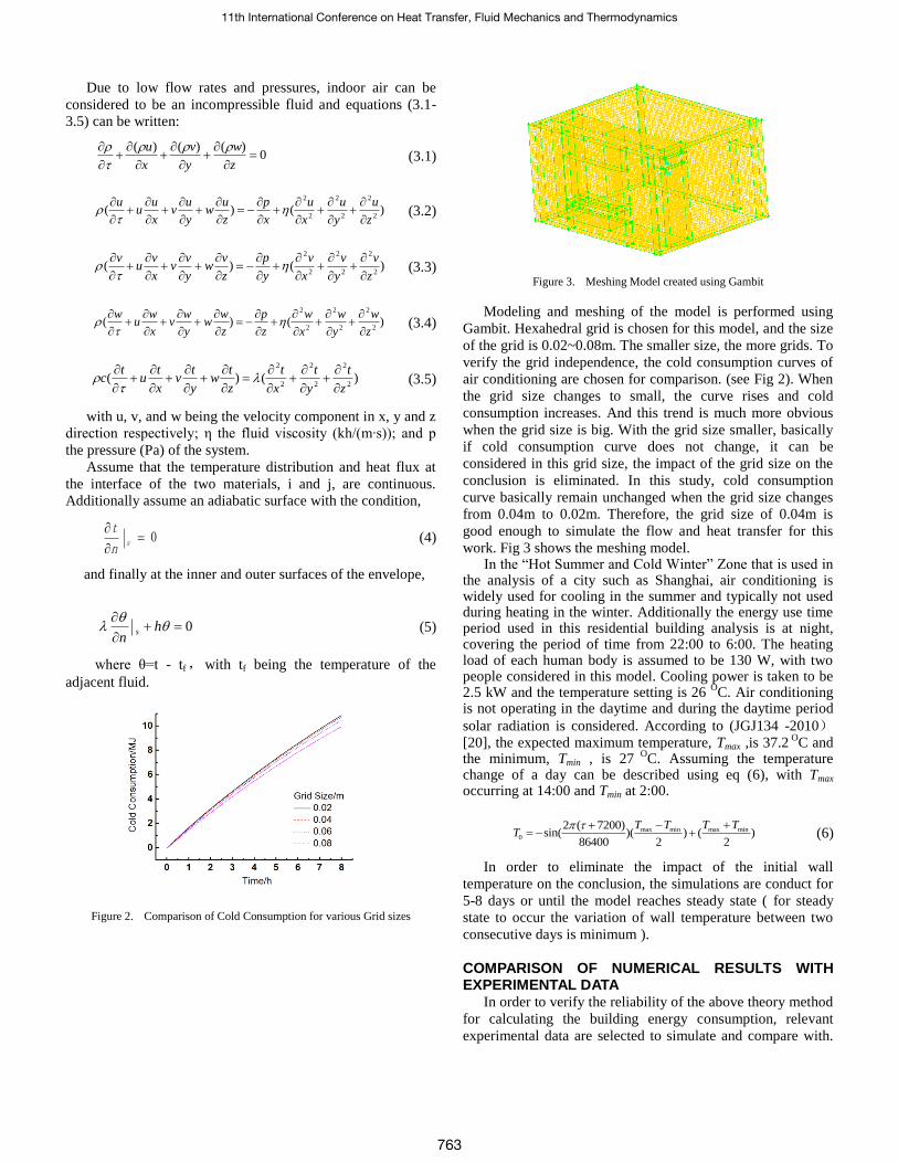
Due to low flow rates and pressures, indoor air can be

considered to be an incompressible fluid and equations (3.1-

3.5) can be written:

0)()()(

z

w

y

v

x

u

(3.1)

)()(2

2

2

2

2

2

z

u

y

u

x

u

x

p

z

uw

y

uv

x

uu

u

(3.2)

)()(2

2

2

2

2

2

z

v

y

v

x

v

y

p

z

vw

y

vv

x

vu

v

(3.3)

)()(2

2

2

2

2

2

z

w

y

w

x

w

z

p

z

ww

y

wv

x

wu

w

(3.4)

)()(2

2

2

2

2

2

z

t

y

t

x

t

z

tw

y

tv

x

tu

tc

(3.5)

with u, v, and w being the velocity component in x, y and z

direction respectively; η the fluid viscosity (kh/(m·s)); and p

the pressure (Pa) of the system.

Assume that the temperature distribution and heat flux at

the interface of the two materials, i and j, are continuous.

Additionally assume an adiabatic surface with the condition,

0

s

n

t (4)

and finally at the inner and outer surfaces of the envelope,

0

h

ns (5)

where θ=t - tf，with tf being the temperature of the

adjacent fluid.

Figure 2. Comparison of Cold Consumption for various Grid sizes

Figure 3. Meshing Model created using Gambit

Modeling and meshing of the model is performed using

Gambit. Hexahedral grid is chosen for this model, and the size

of the grid is 0.02~0.08m. The smaller size, the more grids. To

verify the grid independence, the cold consumption curves of

air conditioning are chosen for comparison. (see Fig 2). When

the grid size changes to small, the curve rises and cold

consumption increases. And this trend is much more obvious

when the grid size is big. With the grid size smaller, basically

if cold consumption curve does not change, it can be

considered in this grid size, the impact of the grid size on the

conclusion is eliminated. In this study, cold consumption

curve basically remain unchanged when the grid size changes

from 0.04m to 0.02m. Therefore, the grid size of 0.04m is

good enough to simulate the flow and heat transfer for this

work. Fig 3 shows the meshing model. In the “Hot Summer and Cold Winter” Zone that is used in

the analysis of a city such as Shanghai, air conditioning is widely used for cooling in the summer and typically not used during heating in the winter. Additionally the energy use time period used in this residential building analysis is at night, covering the period of time from 22:00 to 6:00. The heating load of each human body is assumed to be 130 W, with two people considered in this model. Cooling power is taken to be 2.5 kW and the temperature setting is 26

OC. Air conditioning

is not operating in the daytime and during the daytime period

solar radiation is considered. According to (JGJ134 -2010）[20], the expected maximum temperature, Tmax ,is 37.2

OC and

the minimum, Tmin , is 27 O

C. Assuming the temperature change of a day can be described using eq (6), with Tmax occurring at 14:00 and Tmin at 2:00.

max min max min

0

2 ( 7200)sin( )( ) ( )

86400 2 2

T T T TT

(6)

In order to eliminate the impact of the initial wall

temperature on the conclusion, the simulations are conduct for

5-8 days or until the model reaches steady state ( for steady

state to occur the variation of wall temperature between two

consecutive days is minimum ).

COMPARISON OF NUMERICAL RESULTS WITH EXPERIMENTAL DATA

In order to verify the reliability of the above theory method

for calculating the building energy consumption, relevant

experimental data are selected to simulate and compare with.


763

http://dict.youdao.com/w/solar/

http://dict.youdao.com/w/radiation/

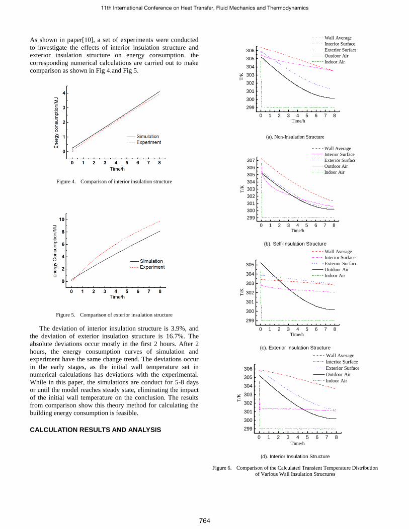
As shown in paper[10], a set of experiments were conducted

to investigate the effects of interior insulation structure and

exterior insulation structure on energy consumption. the

corresponding numerical calculations are carried out to make

comparison as shown in Fig 4.and Fig 5.

Figure 4. Comparison of interior insulation structure

Figure 5. Comparison of exterior insulation structure

The deviation of interior insulation structure is 3.9%, and

the deviation of exterior insulation structure is 16.7%. The

absolute deviations occur mostly in the first 2 hours. After 2

hours, the energy consumption curves of simulation and

experiment have the same change trend. The deviations occur

in the early stages, as the initial wall temperature set in

numerical calculations has deviations with the experimental.

While in this paper, the simulations are conduct for 5-8 days

or until the model reaches steady state, eliminating the impact

of the initial wall temperature on the conclusion. The results

from comparison show this theory method for calculating the

building energy consumption is feasible.

CALCULATION RESULTS AND ANALYSIS

0 1 2 3 4 5 6 7 8

299

300

301

302

303

304

305

306

T/K

Time/h

Wall Average

Interior Surface

Exterior Surface

Outdoor Air

Indoor Air

(a). Non-Insulation Structure

0 1 2 3 4 5 6 7 8

299

300

301

302

303

304

305

306

307

T/K

Time/h

Wall Average

Interior Surface

Exterior Surface

Outdoor Air

Indoor Air

(b). Self-Insulation Structure

0 1 2 3 4 5 6 7 8

299

300

301

302

303

304

305

T/K

Time/h

Wall Average

Interior Surface

Exterior Surface

Outdoor Air

Indoor Air

(c). Exterior Insulation Structure

0 1 2 3 4 5 6 7 8

299

300

301

302

303

304

305

306

T/K

Time/h

Wall Average

Interior Surface

Exterior Surface

Outdoor Air

Indoor Air

(d). Interior Insulation Structure

Figure 6. Comparison of the Calculated Transient Temperature Distribution

of Various Wall Insulation Structures


764

app:ds:in%20the%20early%20stages

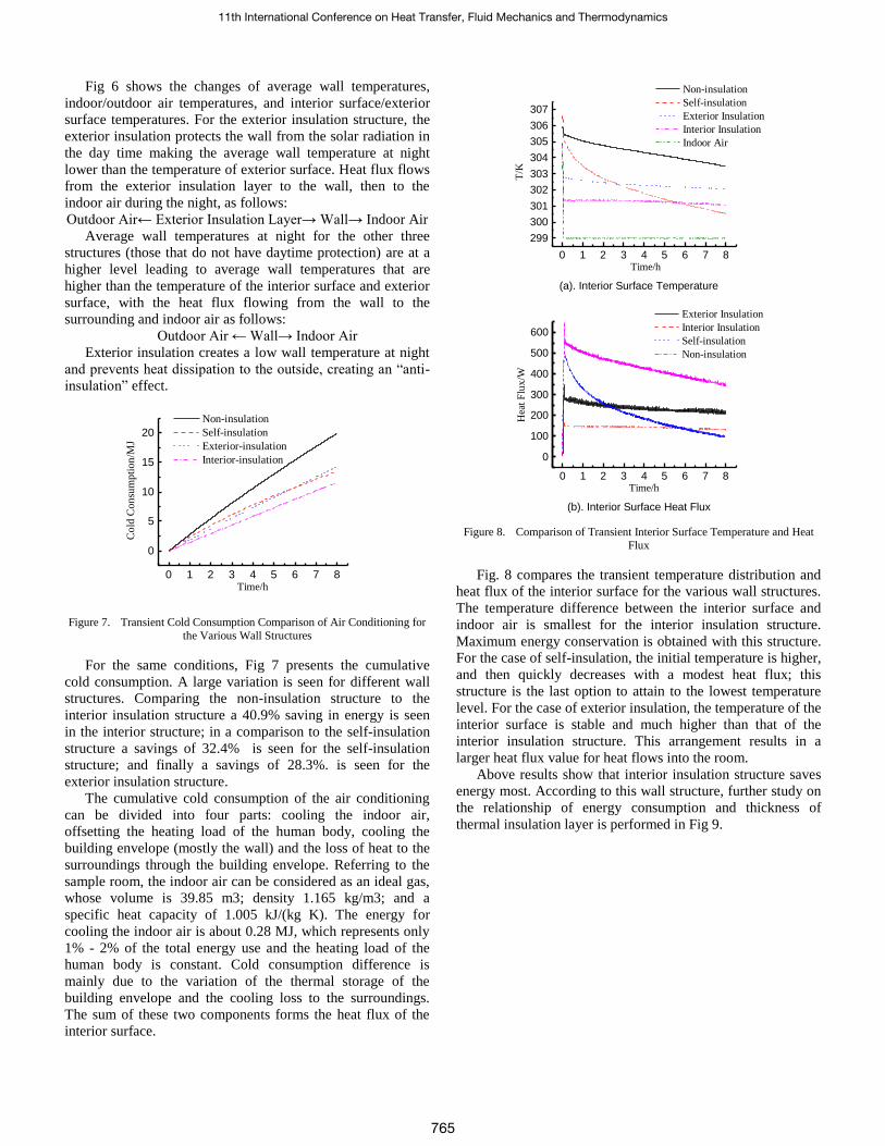
Fig 6 shows the changes of average wall temperatures,

indoor/outdoor air temperatures, and interior surface/exterior

surface temperatures. For the exterior insulation structure, the

exterior insulation protects the wall from the solar radiation in

the day time making the average wall temperature at night

lower than the temperature of exterior surface. Heat flux flows

from the exterior insulation layer to the wall, then to the

indoor air during the night, as follows:

Outdoor Air← Exterior Insulation Layer→ Wall→ Indoor Air

Average wall temperatures at night for the other three

structures (those that do not have daytime protection) are at a

higher level leading to average wall temperatures that are

higher than the temperature of the interior surface and exterior

surface, with the heat flux flowing from the wall to the

surrounding and indoor air as follows:

Outdoor Air ← Wall→ Indoor Air

Exterior insulation creates a low wall temperature at night

and prevents heat dissipation to the outside, creating an “anti-

insulation” effect.

0 1 2 3 4 5 6 7 8

0

5

10

15

20

Co

ld C

on

sum

pti

on

/MJ

Time/h

Non-insulation

Self-insulation

Exterior-insulation

Interior-insulation

Figure 7. Transient Cold Consumption Comparison of Air Conditioning for

the Various Wall Structures

For the same conditions, Fig 7 presents the cumulative

cold consumption. A large variation is seen for different wall

structures. Comparing the non-insulation structure to the

interior insulation structure a 40.9% saving in energy is seen

in the interior structure; in a comparison to the self-insulation

structure a savings of 32.4% is seen for the self-insulation

structure; and finally a savings of 28.3%. is seen for the

exterior insulation structure.

The cumulative cold consumption of the air conditioning

can be divided into four parts: cooling the indoor air,

offsetting the heating load of the human body, cooling the

building envelope (mostly the wall) and the loss of heat to the

surroundings through the building envelope. Referring to the

sample room, the indoor air can be considered as an ideal gas,

whose volume is 39.85 m3; density 1.165 kg/m3; and a

specific heat capacity of 1.005 kJ/(kg K). The energy for

cooling the indoor air is about 0.28 MJ, which represents only

1% - 2% of the total energy use and the heating load of the

human body is constant. Cold consumption difference is

mainly due to the variation of the thermal storage of the

building envelope and the cooling loss to the surroundings.

The sum of these two components forms the heat flux of the

interior surface.

0 1 2 3 4 5 6 7 8

299

300

301

302

303

304

305

306

307

T/K

Time/h

Non-insulation

Self-insulation

Exterior Insulation

Interior Insulation

Indoor Air

(a). Interior Surface Temperature

0 1 2 3 4 5 6 7 8

0

100

200

300

400

500

600

Hea

t F

lux

/W

Time/h

Exterior Insulation

Interior Insulation

Self-insulation

Non-insulation

(b). Interior Surface Heat Flux

Figure 8. Comparison of Transient Interior Surface Temperature and Heat

Flux

Fig. 8 compares the transient temperature distribution and

heat flux of the interior surface for the various wall structures.

The temperature difference between the interior surface and

indoor air is smallest for the interior insulation structure.

Maximum energy conservation is obtained with this structure.

For the case of self-insulation, the initial temperature is higher,

and then quickly decreases with a modest heat flux; this

structure is the last option to attain to the lowest temperature

level. For the case of exterior insulation, the temperature of the

interior surface is stable and much higher than that of the

interior insulation structure. This arrangement results in a

larger heat flux value for heat flows into the room.

Above results show that interior insulation structure saves

energy most. According to this wall structure, further study on

the relationship of energy consumption and thickness of

thermal insulation layer is performed in Fig 9.


765

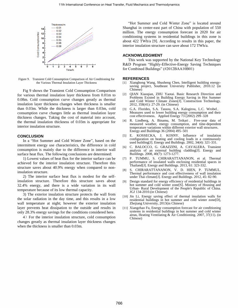
Figure 9. Transient Cold Consumption Comparison of Air Conditioning for

the Various Thermal Insulation Layer Thickness

Fig 9 shows the Transient Cold Consumption Comparison

for various thermal insulation layer thickness from 0.01m to

0.08m. Cold consumption curve changes greatly as thermal

insulation layer thickness changes when thickness is smaller

than 0.03m. While the thickness is larger than 0.03m, cold

consumption curve changes little as thermal insulation layer

thickness changes. Taking the cost of material into account,

the thermal insulation thickness of 0.03m is appropriate for

interior insulation structure.

CONCLUSION

In a “Hot Summer and Cold Winter Zone”, based on the

intermittent energy use characteristics, the difference in cold

consumption is mainly due to the difference in interior wall

surface heat flux. The following conclusions are determined:

1) Lowest values of heat flux for the interior surface can be

achieved for the interior insulation structure. Therefore this

structure saves about 40.9% energy when compared to non-

insulation structure.

2) The interior surface heat flux is modest for the self-

insulation structure. Therefore this structure saves about

32.4% energy, and there is a wide variation in its wall

temperature because of its low thermal capacity.

3) The exterior insulation structure protects the wall from

the solar radiation in the day time, and this results in a low

wall temperature at night; however the exterior insulation

layer prevents heat dissipation to the outside and results in

only 28.3% energy savings for the conditions considered here.

4）For the interior insulation structure, cold consumption

changes greatly as thermal insulation layer thickness changes

when the thickness is smaller than 0.03m.

“Hot Summer and Cold Winter Zone” is located around

Shanghai in center-east part of China with population of 550

million. The energy consumption forecast in 2020 for air

conditioning systems in residential buildings in this zone is

about 422 TWh/a [9]. According to results in this paper, the

interior insulation structure can save about 172 TWh/a.

ACKNOWLEDGMENT

This work was supported by the National Key Technology

R&D Program “Highly-Effective-Energy Saving Techniques

for Combined Buildings” (#2012BAA10B01)

REFERENCES [1] Xianghong Wang, Shusheng Chen, Intelligent building energy-

saving project, Southeast University Publisher, 2010.12 (in Chinese)

[2] QIAN Xiaoqian, ZHU Yaotai. Basic Research Direction and Problems Existed in Building Energy Saving in Hot Summer and Cold Winter Climate Zones[J]. Construction Technology. 2012, 358(41): 27-29. (in Chinese)

[3] G.A. Florides, S.A. Tassou, S.A. Kalogirou, L.C. Wrobel，Measures used to lower building energy consumption and their cost effectiveness，Applied Energy 73 (2002) 299–328

[4] R. Lindberg, A. Binamu, M. Teikari ， Five-year data of measured weather, energy consumption, and time-dependent temperature variations within different exterior wall structures，Energy and Buildings 36 (2004) 495–501

[5] E. KOSSECKA, J. KOSNY. Influence of insulation configuration on heating and cooling loads in a continuously used building[J]. Energy and Buildings. 2002, 34(4): 321-331.

[6] C. BALOCCO, G. GRAZZINI, A. CAVALERA. Transient analysis of an external building cladding[J]. Energy and Buildings. 2008, 40(7): 1273-1277.

[7] P. TUMMU, S. CHIRARATTANANON, et al. Thermal performance of insulated walls enclosing residential spaces in Thailand[J]. Energy and Buildings. 2013, 61: 323-332.

[8] S. CHIRARATTANANON, V. D. HIEN, P. TUMMUL. Thermal performance and cost effectiveness of wall insulation under Thai climate[J]. Energy and Buildings. 2012, 45: 82-90.

[9] Design standard for energy efficiency of residential buildings in hot summer and cold winter zone[S]. Ministry of Housing and Urban- Rural Development of the People's Republic of China. JGJ 134-2010.(in Chinese)

[10] Jin Li, Energy saving effect of thermal insulation walls for residential buildings in hot summer and cold winter zone[D], Zhejiang University, 2013(in Chinese)

[11] Xiangzhao Fu, Energy consumption forecast for air conditioning systems in residential buildings in hot summer and cold winter areas, Heating Ventilating & Air Conditioning. 2007, 37(11). (in Chinese)


766

http://dict.cnki.net/dict_result.aspx?searchword=%e5%9f%8e%e4%b9%a1&tjType=sentence&style=&t=urban+and

Documents

AN INVESTIGATION OF PRODUCE COOLING TUNNEL …