Embed Size (px)
Citation preview

AN INVESTIGATION OF NUGGET FORMATION ANDSIMULATION IN RESISTANCE SPOT WELDING
By
Richard M. Obert
B.S., Mechanical EngineeringRensselaer Polytechnic Institute, 1999
Submitted to the Department of Mechanical Engineeringin Partial Fulfillment of the Requirements for the Degree of
MASTERS OF SCIENCE IN MECHANICAL ENGINEERING
At the
MASSACHUSETTS INSTITUTE OF TECHNOLOGY
June 2001
9 2001 Massachusetts Institute of TechnologyAll Rights Reserved
Signature of Author:.Richard M. Obert
Department of Mechanical EngineeringMay 11, 2001
Certified by:Jung-Hoon Chun
Associate Professor of Mechanical EngineeringThesis Supervisor
Accepted by:Ain A. Sonin
Professor of Mechanical EngineeringChairman, Department Committee on Graduate Students
MASSACHUSETTS INtSTITUTEOF TECHNOLOGY
JUL 16 2001
LIBRARIES
BARKER
AN INVESTIGATION OF NUGGET FORMATION ANDSIMULATION IN RESISTANCE SPOT WELDING
By
Richard M. Obert
Submitted to the Department of Mechanical Engineeringon May 11, 2001 in Partial Fulfillment of the Requirements for the Degree of
Masters of Science in Mechanical Engineering
ABSTRACT
Resistance spot welding is an important part of the automotive manufacturingindustry. Today's automobiles typically contain five-thousand or more welds. Spotwelding is attractive to the industry for its speed and relative simplicity, however, it is notwithout its disadvantages. Current spot welding technology relies on volumes ofempirical data to set the welding parameters. Often this data is not sufficient to ensurethat a nugget of sufficient size is formed without a splash occurring. Complicating thematter further is the industry's increased use of coated steel. The chemical reaction of thecoatings with the electrodes cause greater variations in the nugget size.
This study seeks to characterize the nugget formation patterns of spot welding fora variety of welding materials and welding conditions. Specifically for coated steelswelded over long periods with the same electrodes. The study also seeks to relate a smallset of monitored parameters during welding to the accurate prediction of nugget size andsplash occurrence. Welding current and voltage are identified as the key parameters ofinterest and are used as input to a numerical simulation to predict nugget diameter. Acomparison of the simulated nugget diameters to actual diameters obtainedexperimentally show good agreement between the two values. The simulation, however,uses a finite difference method to obtain the nugget diameter. This method requiresextensive calculations that cannot be completed in the normal welding time. Therefore, anew method of splash prediction has been investigated using the mean temperature of theworkpiece. The mean temperature is obtained from a heat balance model of theworkpiece. The heat balance model is advantageous to the finite difference simulationbecause its calculation time is short enough to be carried out during the welding process.A comparison of the maximum mean temperature and the experimental nugget diametersshows that mean temperature is capable of predicting nugget diameter. This correlationindicates that the mean temperature value can serve as a splash prediction parameter.
Thesis Supervisor: Dr. Jung-Hoon ChunTitle: Associate Professor of Mechanical Engineering
2

Acknowledgements
I would like to thank the people who have assisted me with the completion of this
project. First, I would like to thank my thesis supervisors, Professor Jung-Hoon Chun
and Dr. Kin-ichi Matsuyama for their support and guidance. I am grateful for the time
Dr. Matsuyama spent explaining the background information of spot welding. I also
would like to thank Professor Chun for keeping me focused on the writing of this paper.
To the others who have assisted me along the road to completing this project, especially,
our shop machinists, Gerry Wentworth and Mark Belanger, the Amp Lab technician,
Cheng Su, Yin-Lin Xie from the department of Material Science thank you for your
advice and support.
I would also like to express my gratitude to Kawasaki Robotics corporation and to
Osaka Denki for their support of this project. Also to the Dengensha Mfg. Co., Ltd,
Matsushita Industrial Equipment Co, Ltd, and Nippon Steel Co. thank you for the support
provided.
3
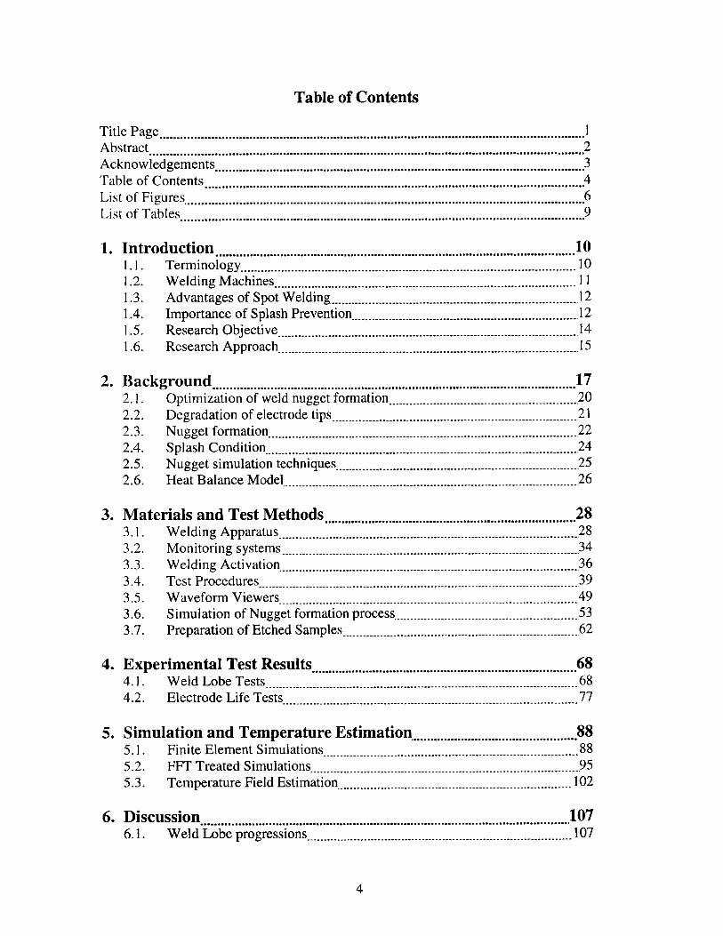
Table of Contents
T itle Page ................................................... ................. ................. ......................Abstract. . .2Acknowledgements .............................................Table of Contents 4List of Figures ................................................. 6List of Tables .. 9
1. Introduction 101.1. Terminology ........ 101.2. Welding Machines ...................................... 111.3. Advantages of Spot Welding ............................... 121.4. Importance of Splash Prevention ............................ 121.5. Research Objective ...................................... 141.6. Research Approach ..................................... 15
2. Background 172.1. Optimization of weld nugget formation ........................ 202.2. Degradation of electrode tips .............................. 212.3. Nugget formation ...................................... 222.4. Splash Condition ...................................... 242.5. Nugget simulation techniques ............................... 252.6. Heat Balance Model 26
3. Materials and Test Methods 283.1. Welding Apparatus ..................................... 283.2. Monitoring systems ..................................... 343.3. Welding Activation ..................................... 363.4. Test Procedures 393.5. Waveform Viewers 493.6. Simulation of Nugget formation process .................. .533.7. Preparation of Etched Samples ......................... .62
4. Experimental Test Results ............................ 684.1. Weld Lobe Tests 684.2. Electrode Life Tests 77
5. Simulation and Temperature Estimation ................. 885.1. Finite Element Simulations 885.2. FFT Treated Simulations 955.3. Temperature Field Estimation 102
6. Discussion._____.. 1076.1. Weld Lobe progressions ................................ 107
4
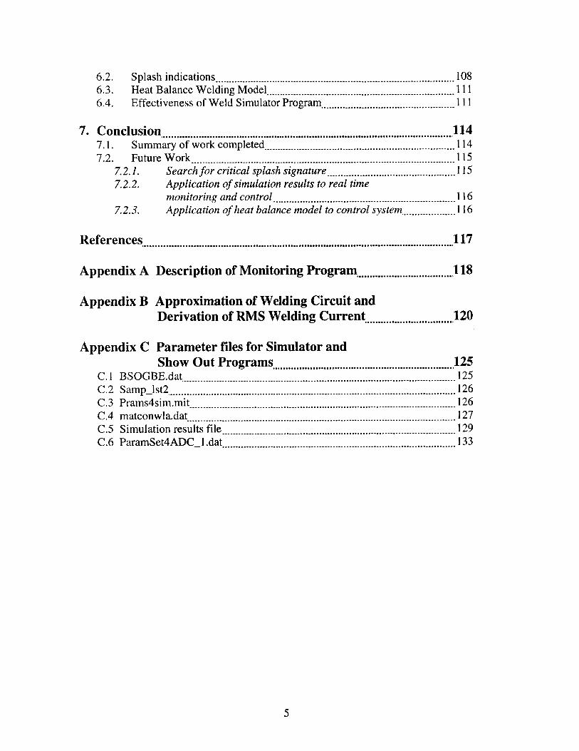
6.2. Splash indications ..................................... 1086.3. Heat Balance Welding Model ............................. 1116.4. Effectiveness of Weld Simulator Program ..................... 11 1
7. Conclusion 1147.1. Summary of work completed ............................. 1147.2. Future Work .115
7.2.1. Search for critical splash signature .................... 1157.2.2. Application of simulation results to real time
monitoring and control ............................ 116
7.2.3. Application of heat balance model to control system ........ 16
References 117
Appendix A Description of Monitoring Program ............ 118
Appendix B Approximation of Welding Circuit andDerivation of RMS Welding Current ... . .. . . .............. 120
Appendix C Parameter files for Simulator andShow Out Programs ........................ 125
C. I BSOGBE.dat 125C.2 Sampjlst2 ........................................... 126C.3 Prams4sim.mit 126C.4 matconwla.dat 127C.5 Simulation results file 129C.6 ParamSet4ADC1 .dat .................................... 133
5

List of Figures
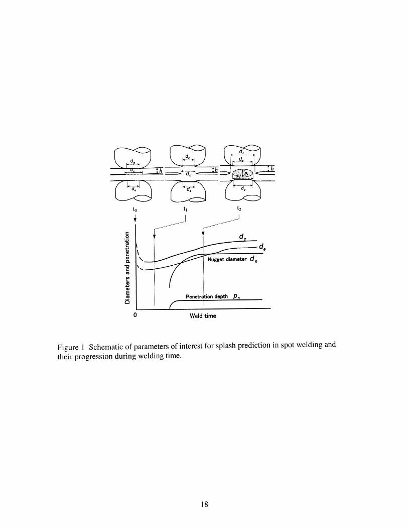
Figure 1 Schematic of welding parameters of interest for splash prediction in 18spot welding and their progression during welding time.
Figure 2 Schematic illustration of spot welding parameters and electric field 19patterns in the workpiece during welding.
Figure 3 Approximation of current path during welding to evaluate the 23resistance between electrode tips: (a) schematic of actual weldingconditions, (b) modeling workpiece as homogeneous rod.
Figure 4 Experimental welding apparatus: (a) photo of apparatus, (b) schematic 29of welding apparatus showing voltage and current monitoring devices.
Figure 5 Schematic of support structure used to hold weld specimens in place 30during welding showing position with respect to specimens andwelding apparatus.
Figure 6 Robotron Series 400 welding controller input panel. 32
Figure 7 User interface of resistance spot welding monitoring program 37(RW Mon by Lab-PC- 1200).
Figure 8 Welding orientation of organic-zinc coated steel sheets during 43electrode life test.
Figure 9 Timeline of test procedures for electrode life test. 45
Figure 10 Tensile test specimen (0.76 mm (0.03 in.) thickness). 47
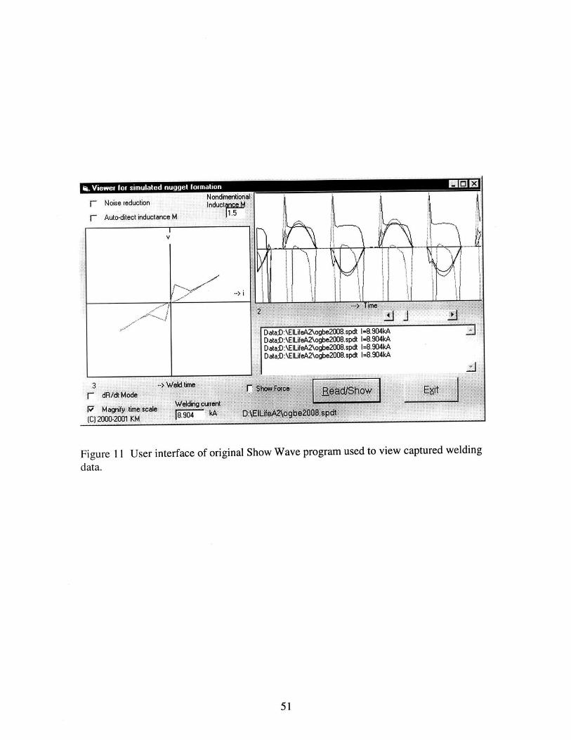
Figure 11 User interface of original ShowWave program used to view captured 51welding data.
Figure 12 User interface of Monitoring Data Extraction program used to 52calculate the gain value for current input or the RMS current.
Figure 13 User interface of simulation results viewer used to graphically display 59the results of finite element simulations of welding conditions.
Figure 14 User interface of updated Show Wave program using FFT treatment. 61
Figure 15 Cutting steps to observe cross section of weld nugget: (a) coarse cut 63to isolate nugget, (b) coarse cut to reduce specimen width(c) fine cut to reveal center cross section of nugget.
6

Figure 16 Nugget diameter vs. welding current. Weld lobe test results: welding 70time of 10 cycles, old dome electrodes used with pneumatic weldinggun on galvannealed steel.
Figure 17 Waveform of monitoring data taken during splash condition in the 71weld lobe tests.
Figure 18 Nugget diameter vs. welding current. Weld lobe test results: welding 73time of 10 cycles, old dome electrodes used with pneumatic weldinggun on organic-zinc coated steel.
Figure 19 Nugget diameter vs. welding current. Weld lobe test results: welding 74time of 10 cycles, new dome electrodes used with pneumatic weldinggun on galvannealed steel.
Figure 20 Nugget diameter vs. welding current. Weld lobe test results: welding 75time of 10 cycles, new dome electrodes used with servo weldinggun on galvannealed steel.
Figure 21 Nugget diameter vs. welding current for weld lobes taken during the 78electrode life test.
Figure 22 Tensile force vs. welding current for weld lobes taken during the 79electrode life test.
Figure 23 Weld diameter vs. tensile force for weld lobes taken during the 80electrode life test.
Figure 24 Current levels of minimum nugget formation, acceptable nugget 82formation and splash condition for each weld lobe test conductedduring the electrode life test.
Figure 25 Difference between critical nugget formation current and splash 83condition current over the course of the electrode life test.
Figure 26 Tip diameter vs. weld number for electrode life test. 85
Figure 27 Photographs of etched cross-section of weld nugget showing nugget 87boundary and heat affected zone changing over welding time.Welding current of 4.40 kA and a welding force of 200 daN were usedfor all samples: (a) welding time 8 cycles, (b) welding time 10 cycles,and (c) welding time 12 cycles.
Figure 28 Nugget diameters as a function of A, in the simulation program. 94
Figure 29 Monitoring waveform with: (a) properly chosen value of mutual 96
7
inductance and (b) poorly chosen value of mutual inductance.
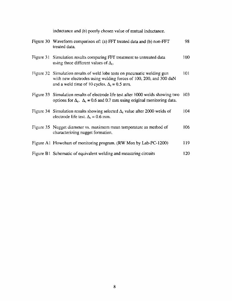
Figure 30 Waveform comparison of: (a) FFT treated data and (b) non-FFT 98treated data.
Figure 31 Simulation results comparing FFT treatment to untreated data 100using three different values of Ac.
Figure 32 Simulation results of weld lobe tests on pneumatic welding gun 101with new electrodes using welding forces of 100, 200, and 300 daNand a weld time of 10 cycles. A, = 0.5 mm.
Figure 33 Simulation results of electrode life test after 1000 welds showing two 103options for Ac. A, = 0.6 and 0.7 mm using original monitoring data.
Figure 34 Simulation results showing selected Ac value after 2000 welds of 104electrode life test. Ac = 0.6 mm.
Figure 35 Nugget diameter vs. maximum mean temperature as method of 106characterizing nugget formation.
Figure A l Flowchart of monitoring program. (RW Mon by Lab-PC- 1200) 119
Figure B 1 Schematic of equivalent welding and measuring circuits 120
8
List of Tables
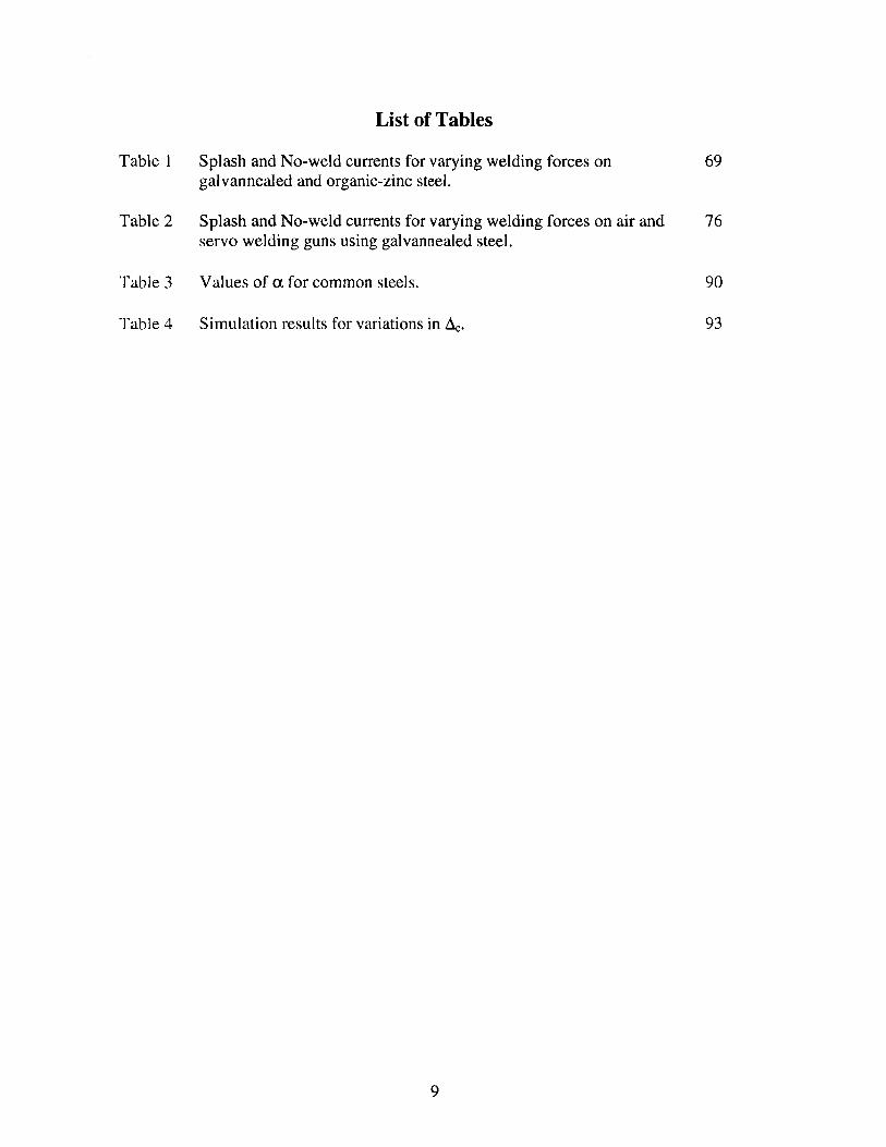
Table I Splash and No-weld currents for varying welding forces on 69galvannealed and organic-zinc steel.
Table 2 Splash and No-weld currents for varying welding forces on air and 76servo welding guns using galvannealed steel.
Table 3 Values of a for common steels. 90
Table 4 Simulation results for variations in Ac. 93
9

Chapter 1Introduction
Spot welding is a process in which a number of pieces of material are joined
together by melting the material at the intervening, or faying surface, of the specimens.
This melting forms a solid nugget that binds the specimens together. Melting is achieved
by compressing the specimens between two electrodes and passing a current through the
electrodes and material. The nugget size depends on the magnitude of the current, the
electrode force, and the length of time that the current is applied to the specimens. If the
parameters are not chosen carefully, expulsion of molten material may occur during the
welding process. It has proven difficult to predict the occurrence of this expulsion
phenomenon. In order to study this process more carefully, a welding apparatus has been
configured to monitor critical welding parameters in real time. This apparatus has been
used to obtain experimental data which was used to verify the accuracy of various
welding models.
1.1 Terminology
The automotive industry has established some common terminology that can be
used when describing the spot welding process. This includes references to the welding
apparatus, welding parameters, and welding specimens. To start, the apparatus used for
spot welding is often called a welding gun. It can be modified by the type of actuator
used. In this investigation two types of welding guns were used. The first is controlled
by air pressure and will be referred to as an air gun. The second uses a servo motor and
will be referred to as a servo gun. The actuator, in either case, controls the position of,
10
and force applied by the electrode tips. These are the parts of the welding apparatus that
actually make contact with the material to be welded. They are typically made of copper,
because of its high electrical and thermal conductivity. When the electrodes contact the
specimen there is a slight deformation of the electrode tip. This results in a larger contact
area between the tips and specimens than would be found by simply measuring the
electrode face diameter. This contact is referred to as the electrode diameter and is
typically assumed to be circular. The force with which the electrodes are pressed
together is called the electrode force. This force causes an area on the contacting surfaces
of the specimens to be pressed very close together. This area is defined as the contact
diameter. The entire surface between two specimens, where the weld will form, is called
the faying surface.
The metal first begins to melt at this surface within the contact diameter. The
metal that melts, and subsequently solidifies to bond the specimens, is know as the weld
nugget. The nugget has two critical dimensions. The first is the nugget diameter which is
represented by the width of the nugget at the faying surface. The second is the
penetration depth which is the overall height of the nugget at its center. The area around
the nugget that has had its microstructure changed due to the heat of welding is known as
the heat affected zone (HAZ). A current must be passed through the electrodes to cause
the heating and melting of the specimens necessary for nugget formation. This current is
specified by the operator and is called the welding current, the duration that the current is
applied to the specimens is called the weld time.
11
1.2 Welding Machines
There are various types of welding machines used in industry today. Their size
and shape depends on their intended application. Many machines in the automotive
industry are mounted on robotic manipulator arms to move about the body of a vehicle
during assembly. Welding machines can be built for use with either DC or AC currents.
The automotive industry predominantly uses AC machines. For this investigation two
welding machines were used. Detailed descriptions of these machines and their operation
can be found in Chapter 3.
1.3 Advantages of Spot Welding
Spot welding provides many benefits over other existing welding techniques.
One of its greatest benefits is that it does not require additional material to form a weld.
The nugget formed is a combination of the material from the specimens to be welded. In
most other welding processes, such as arc-welding and metal-inert gas (MIG) welding, a
wire or rod of material must be fed into the weld area to have enough material to form a
weld. Additionally, attaching sheets of metal together is faster with spot welding because
only certain areas need to be welded to establish the necessary bond strength.
1.4 Importance of Splash Prevention
Splash prevention is very important to the automotive industry. There are several
negative effects of the splash phenomenon that make its elimination extremely important
to the improvement of the overall welding process. The detrimental effects of expulsion
12

can be separated into three categories: the effect on the manufacturing process and
equipment, the effect on the electrode tips, and the effect on nugget formation.
When a splash takes place, the molten metal at the faying surface is no longer
contained by the surrounding solid metal. The force of the electrode tips cause this metal
to spray out from between the specimens. When the spray reaches the surrounding air at
room temperature it solidifies quickly into very tiny pellets. The pellets are usually on
the order of 0.45 mm in diameter. Some droplets will attach to the welded material
before solidifying, while others will continue to fly out from the specimen into the
surrounding workspace. In either case, the effects are detrimental to the manufacturing
process. In the first case, the metal that has attached to the specimen must often be
removed. This involves a expensive and time consuming grinding and polishing step. If
the metal is not removed it may negatively effect future welds or future steps of the
assembly process. In the second case, this material can easily become lodged in the
many moving parts of the equipment in the welding area. Over time these particles can
build up on moving parts and cause increased wear and downtime of the equipment.
The splash condition in typical welding configurations represents an overheating
condition due either to excessive welding current or welding time. This overheating
extends to the outer surfaces of the weld specimens. Since the primary method of heat
removal from the welded part is through the electrode tips, this additional heat is
eventually carried to the tips. The combination of increased temperature at the outer
surface and electrode tip contact produces increased electrode tip wear for two reasons.
First, the increased heat acts to soften the electrode material. This causes increased
deformation of the tip. This deformation can lead to unacceptable welds as a larger tip
13

will have a smaller current density and will produce a smaller weld under the same
welding conditions. Second, in coated steels which are used widely in the automotive
industry, there is a chemical reaction that occurs between the electrode tip and the surface
coating. A zinc alloy and copper are the typical materials for the coating and the
electrode tips, respectively. These two metals react with each other to form a coating of
brass on the electrode. The material properties of brass are not as favorable for welding
as those of copper. The conductivity, both electrical and thermal, is much lower for brass
and will produce poorer welds as a result. The reaction between these two metals is
related to the temperature of each of them. When they contact at a higher temperature the
reaction rate is increased and performance is rapidly reduced. It is possible to reach a
point where the electrode tips have become coated with enough brass that an acceptable
nugget can no longer be formed. While both of these cases represent normal wear of the
electrode, the increased heat generated in the splash condition accelerates this wear. This
leads to more frequent changes of the electrode tips which requires the machine to be
shut down.
Finally, the metal expelled during the splash comes from the pool of molten metal
between the specimens. Since the weld is formed from the existing material, any metal
that is lost to expulsion is no longer available to form the nugget. This generally results
in a smaller nugget being formed between the specimens. If the splash is large enough,
the nugget that is formed will not have sufficient dimensions in diameter and height.
This leads to problems in the manufacturing line, as a significant number of extra welds
must be made. This is done to ensure that enough quality welds have been produced.
14

1.5 Research Objectives
The goal of this investigation was to identify possible methods for controlling the
process to avoid the splash condition in resistance spot welding. The results of this study
will be used to identify critical parameters to be used in future quality monitoring and
control routines for resistance spot welding.
1.6 Research Approach
To achieve this objective, it was first necessary to obtain welding data that would
characterize the various welding conditions that might be encountered in an industrial
setting. This data consisted of both the physical weld specimens produced and the
current, voltage, and force data taken during the welding process. The data was first
examined in an attempt to find any characteristics that could be used as an indicator of an
impending splash. Since the data alone did not produce any such indicator, it was used as
input to a finite element program. The results of this program were compared to the
actual experimental results of the welds to verify the program's accuracy. After the
program was proven to be accurate, the results were examined for feasibility of use in a
control routine. It was expected that if the results of a finite element simulation proved
accurate, the time required to produce these results would not be acceptable for a
real-time control mechanism. Therefore, it was intended that the results of the simulation
be used as further verification of future control routines that would be developed. The
final focus of this investigation involves the verification of one of these welding models.
The model uses the heat balance equation of a welded part to predict the mean
temperature of the weld. It is believed that there is a characteristic mean temperature
15

during welding, beyond which splash will occur.
final step of this investigation.
16
The verification of this model is the

Chapter 2Background
Spot welding has been used for many decades in the automotive industry as an
efficient and inexpensive method of joining components of an automobile together. The
average cost of a single weld is approximately $0.05. However, a typical car body
contains several thousand welds. This large number of welds begins to increase the price
associated with the manufacturing of the automobile. In recent years, automakers have
changed the typical materials used in the frames of automobiles, preferring a coated
material to the bare steel originally used. The coated material is chosen for its improved
corrosion resistance. However, the typical coatings used, some form of zinc or zinc
alloy, have been found to cause increased wear on the electrode tips. This doubly effects
the cost of manufacturing as tips must be replaced more often and welding results
become more difficult to estimate requiring more welds to be made to insure a specified
number of quality welds are made [1].
Welding machines used in industry are almost entirely alternating current (AC)
machines. These machines are chosen for their simple component make up compared to
direct current (DC) machines. Since most supply lines today carry AC power, it is much
easier to achieve the necessary currents and voltages without converting to DC. A typical
welding machine is described in detail in Chapter 3. Figure 1 shows the standard
parameters of interest in the welding process. Figure 2 shows the electrical fields seen in
the weld specimen during welding.
17
d
to Li t
C - j
--- d,
CL Nugget diameter d,
MC
4j,
E. Penetration depth p,
0 Weld time
Figure 1 Schematic of parameters of interest for splash prediction in spot welding and
their progression during welding time.
18

Electrode-
Figure 2 Schematic illustration of spot welding parameters and electric field patterns inthe workpiece during welding.
19
2.1 Optimization of weld nugget formation
The procedures used to obtain quality welds rely heavily on the evaluation of
physical attributes of the weld. These attributes are measured over some time interval
and compared to existing welding data. The existing data is used to identify what
welding conditions are present and to suggest the correction needed if unsatisfactory
welds are being produced. If it is found that the unsatisfactory nuggets are being
produced, the data will indicate what process variables should be adjusted to get the
desired nugget size [2]. To ensure accurate nugget size control throughout the welding
process, continuous monitoring of the weld formation process is needed [3]. This
requires that several test welds be broken to obtain experimental nugget information.
This test weld must be created instead of making a structural weld. The test weld also
requires special test specimens because the sample must be destroyed to obtain the data
needed. This requires extra time, for the set up of the different specimen. It also
increases the cost of the materials, as the specimens must be separate from the rest of the
automotive structure. The difficulties associated with determining the appropriate
welding parameters have been further complicated by the increased use of coated steel
sheets in the automotive industry. The coating produces greater variation in the quality
of the nugget produced. Often, a trial and error process is relied upon to obtain
satisfactory welds.
2.2 Degradation of electrode tips
While better for corrosion resistance, it has been observed that the use of coated
steel sheets causes increased wear on the electrode tips. Coated steel causes tip
20

degradation to occur on the order of one hundred times faster than bare steel sheets. This
contributes to a significant amount of time lost, in order to change electrodes on the
welding machines. Experiments were conducted by Dupuy, et al. to characterize this
wear. Their results showed that the electrode is consumed by a chemical reaction with
the coating more than it is deformed from the heat and stress of welding. The electrode
consumption is caused by the formation and subsequent elimination of intermetallics.
These intermetallics consist of some binary form of copper from the electrode and the
coating material. Since zinc, or one of its alloys, is a widely used coating, brass is one of
the most commonly formed intermetallics. The formation of intermetallics is not uniform
across the electrode tip. Therefore, certain areas can have deeper loss of material than
others. This phenomenon is known as pitting. Pitting not only changes the shape of the
electrode but also causes a reduction in contact between the electrodes and the specimen.
In some cases, the formation of these intermetallics can cause sticking between the
electrode tips and the weld specimen. The actual effects of electrode degradation are
extremely hard to predict. The entire process depends on the welding conditions,
welding rate, and the coating used. Since most welding tables were originally made
before coated steels were being used, poor welds are often made. These unsatisfactory
welds are created because degradation effects were not accounted for in the selection of
the welding conditions [1].
2.3 Nugget formation
The nugget formation process in resistance spot welding is caused by the heat
generation of current passing through a resistor. The resistance is directly related to the
21

resistivity of the weld material. The current density, the current divided by the area
through which the current flows, is also important in the nugget formation process. The
electrode degradation would not be as serious an issue if not for the importance of the
current density. The electrode tip degradation described above contributes to a larger
electrode tip contact area. This causes the current, assumed to be a constant value, that
passes through the electrode tip to be spread over a larger area. Therefore, it is the
current density rather than the actual current value that cause the discrepancies in
predicted and actual nugget diameters. The effects of varying current density are
determined by the diameter of the current path estimated as a rod. Therefore the current
density is proportional to the resistance of the rod, given as
R = 1
e
where p is the resistivity of the workpiece, 1 is the thickness of the welded area, and de is
the electrode contact diameter.
This is illustrated in Figure 3 which shows the actual welding setup in part a and
the approximation of the current path as a rod in part b.
Several studies have also been conducted to determine what differences exist
between AC and DC welding conditions. These results concluded that current
fluctuation, seen in AC welding, has an effect on nugget formation and nugget
temperature. This fluctuation causes a corresponding fluctuation in both diameter and
temperature. However, the final resultant nugget is found to be nearly identical for AC
and DC welding machines [4]. Further studies in AC and DC current sources found that
the effect of current fluctuation is dependent of the thickness of the material being
welded. The fluctuation was determined to be significant when using sheets thinner than
22

1 Rod
(b)(a)
Figure 3 Approximation of current path during welding to evaluate the resistance
between electrode tips: (a) schematic of actual welding conditions, (b) modeling
workpiece as homogeneous rod.
23
Electrodel
\idPlate
Current !path d

1.0 mm. In contrast, the effects of fluctuation were determined to be negligible in
specimens greater than 1.5 mm thick [4].
Another cause of concern in modeling the nugget formation process is the role of
contact resistance. Contact resistance is defined as the resistance between the electrode
tips and the specimens. It was perceived to be a greater issue with the use of coated
steels, because the coating causes an increase in the contact resistance. Models and
prediction methods were created to include the effects of this resistance. A recent study
was conducted in which two models were compared to experimental results. The first
model included the effect of contact resistance while the second did not. Contrary to
earlier beliefs, it was found that the results from both models accurately represented the
experimental results. Therefore, it was concluded that the contact resistance effects could
be ignored when considering the nugget formation [5].
2.4 Splash Condition
Researchers in the field of resistance spot welding have been trying for some time
to determine an acceptable model for the occurrence of expulsion. One model, proposed
by Browne, et al, describes a contact diameter at the faying surface. The model predicts
that splash will occur when the nugget diameter exceeds this contact diameter. A second
model, developed by Senkara et al., proposes that expulsion occurs when the force caused
by the melting of the metal in the nugget exceeds the containment force applied by the
electrodes [6]. However, there are some caveats to each of these models. Most important
is the large amount of calculation and information required to accurately estimate these
models. The calculations must either be more rigorous or the approximation will have a
24
greater error, especially in the case of irregularities in the geometry. Additionally, these
models have not proven to be entirely accurate in predicting splash occurrences. Most
importantly, expulsions have been observed in which the nugget had not yet exceeded the
contact diameter.
Another problem facing many of the proposed models is that, in AC welding, the
critical expulsion current decreases because of temperature fluctuation in the corona bond
area. This area is the non-melted zone that surrounds the nugget during formation [4].
After completing a weld this area would be considered the heat-affected zone (HAZ).
The corona bond area would include the non-melted region described in the Alcan model,
while the nugget diameter remained less than the contact diameter. The temperature
fluctuation is a direct result of the current fluctuation. A third model, then seeks to
describe the splash as the result of the weld part being overheated [3]. This overheated
state causes a sudden melting of the corona bond area that breaks down the containment
structure surrounding the molten nugget. Without containment, the metal is free to flow
out into the surroundings.
2.5 Nugget Formation Simulation Techniques
Several researchers have successfully developed simulation procedures that can
predict nugget diameters. A real time monitoring system has been developed to be used
in conjunction with a simulation program to simulate nugget diameters. This system has
been shown to produce good results for welds with both new and old electrode tips.
However, as with most simulation programs, a long calculation time is needed to obtain
the results. This calculation time is often on the order of 100-1000 times the actual weld
25

duration [7]. As a result, this process cannot be applied to real time control or prediction
of the welding process. These methods typically use the differential equation form of the
welding model. This is represented in the simulation model using the finite difference
method. To obtain accurate results from the finite difference, finite element, or finite
boundary methods, a large number of mesh points are required. These mesh points
represent the discrete approximation of the simulator to the continuous real-world
problem. The smaller the mesh size and greater number of mesh points, the greater the
accuracy of the simulation. Unfortunately, this accuracy comes at the cost of an
increased number of calculations that contribute directly to the total simulation time [3].
2.6 Heat Balance model
A new method of splash prediction involves the use of the integral form of the
heat balance equation.[8] This concept was developed from the similar work of Okuda.
This type of thermal consideration has been attempted for many years but the results have
never been able to accurately predict the nugget formation [3].
This new model assumes that a mean temperature of the total nugget formation
area can describe the welding state. The heat contained in this area is theoretically given
as [3]:
Q=f v-i.f(dlh)+2K --7-+rdh - dt (2)az 4 I I
where Q is the heat contained in the workpiece, t the time, v the voltage between plate
surfaces, i the welding current, Ke the heat conductivity of electrode tips, K the thermal
conductivity of weld specimens, d the contact diameter between electrode and weld
piece, T the temperature, h, the total plate thickness, f(d/h) the correction factor of current
26

density due to fringing, h the thickness of one plate, r the radius direction, and z the
vertical direction, respectively.
The mean temperature in the weld part is then described as:
T(t) = 34Q
ht Card2 (3)
where Q is the heat contained in the workpiece from Eq. 2, C is the specific heat of the
workpiece, and u the density of the workpiece, respectively.
It has been shown that the effect of heat loss during the welding process is
negligible when considering the temperature [3]. These two results can be combined into
an integral equation for the mean temperature by substitution. It is believed that a
governing parameter for proper welding conditions can be obtained from this equation.
Of further importance is the development of a temperature estimation routine that
can be applied to a real time monitoring system to predict splash occurrence. This
estimation routine is derived from the integral form of the equation and converted into a
discrete form for use with the sampling data. It is necessary to first convert the voltage
and current into volts and amperes respectively. The voltage must then be adjusted to
account for the effects of mutual inductance. The temperature can then be estimated
from the modified voltage.
27

Chapter 3Materials and Test Methods
This section describes the various test procedures and apparatus used in this
investigation. It also details the test materials used.
3.1 Welding Apparatus
A welding apparatus has been designed to conduct the experiments, of various
welding conditions, needed in this investigation. The welding apparatus has been
constructed to represent the typical spot welding machine that is used in industrial
applications. Figure 4a is a photograph of the welding apparatus; Figure 4b shows the
schematic of the welding apparatus and the measurement points. The welding apparatus
applies a force to metal specimens placed between two electrodes. The welding
apparatus then passes a current through the electrodes and material, causing a portion of
the material to melt. This molten material is what will form the weld after it solidifies.
The welding apparatus shuts off the current while still maintaining a pressure on the
specimens. Finally, the applied force is removed from the specimens thus allowing them
to be removed from the apparatus. Water is forced through the interior of the electrodes,
thereby cooling them. The welding apparatus has been modified to enable the
measurement of electrode force, current, and voltage during the welding process. These
measurements were capable of being recorded on a PC using an A/D converter.
For welding the typical 30 mm by 100 mm test coupons, it was necessary to
construct a support platform on which the coupons could be placed and held stationary
during welding. Figure 5 shows a schematic of the support platform and its relative
28

.~ . - . . - . - - . - ..- - .. . . . . --Piston
Welding 4Current
SvwedingMotion
F"V7
(a).............(b)Fig re E perme talwedin a part .:.() .h.t ...ap art.s. (). she ati..
Fgr4Exeietlwelding apparatus:sh(w)nghototag andparatust mbitorcngmdeicces
29

WeldingMotion
.- Workpiece
Aluminum
Electrodes
- Plexiglas
Steel Support
Adjusting Screw
Figure 5 Schematic of support structure used to hold welding specimens in place during
welding.
30

position during welding. The support platform is a four sided rectangular box with holes
centered in the top and bottom. The box can be placed such that the top hole fits over the
bottom electrode of the welding gun and the bottom hole fits over an adjusting screw on
the support structure. Sheets of aluminum 1 mm thick can be added as needed to make
the top surface of the box level with the top surface of the electrode. The box is
constructed from one-half inch thick aluminum on the sides and bottom and one-quarter
inch thick Plexiglas on the top that serves as an insulator.
The welding apparatus consists of three components: a controller, a welding gun,
and an electrode cooling system. Each of these components is discussed in the following
sections.
The welding controller used for the experiments was a Robotron Series 400
Controller. This controller allowed the use of a direct program mode where the welding
parameters could be set directly at the controller. Figure 6 shows the control panel of the
Robotron Series 400. These parameters could be changed after each weld if necessary.
The parameters controlled by this device were weld time and welding current. Additional
parameter settings, not varied in this investigation, included squeeze time and hold time.
It is during these respective interims before and after the weld, that the electrodes apply
force to the specimen while no current is passed through the electrodes.
The welding gun is the portion of the device at which the welding actually takes
place. The welding gun can be further divided into several components and subsystems,
the majority of which are unimportant to this study. The welding gun is typically a
C-shaped device with one fixed end and one movable end. The movable end is attached
to some form of linear actuator. The actuator is required to move the electrode tip into
31

Figure 6 Robotron Series 400 welding controller input panel.
32

contact with the welding specimens and apply the desired welding force to the specimens.
The various types of actuators used in this experiment are discussed in greater detail
below. The C-shaped device is affixed to a large metal structure to provide support. The
support structure is fitted with an adjusting screw. This screw can be raised or lowered
with respect to the lower, immobile, electrode. If desired, the screw can be moved to
contact the bottom of the welding device to provide essentially zero displacement at the
lower electrode. The power source and control signal from the welding controller are
attached to the top of the actuator.
Two types of actuators were used during the course of this investigation. The first
is powered by air pressure and is typically found in industrial applications. The second
type is operated by a servo motor and was being tested for some of its improved
characteristics. The air powered actuator is controlled by adjusting a pressure regulator
until the desired electrode force is obtained. When activated, the air pressure is applied to
a piston attached to the upper electrode. This causes the electrodes, and any intervening
material to be pressed together at the desired force. The servo motor actuator is
controlled using a Dengensha Servo Spot Gun controller. The desired force must be set
through a computer program and is passed to the controller through a PC card interface.
There are some important differences between the two actuators. Generally, the
servo motor is a faster actuator. It responds much faster to the weld signal, as it does not
have the delay introduced by the air pressure. However, this can produce negative
results, especially at higher welding forces. The increased speed, in this case, translates
into an increased impact force that can lead to rapid tip wear and deformation. However,
33

an advantage of the speed of the servo motor, in conjunction with PC control, is the
ability to change the electrode force during the welding cycle.
The electrode cooling system consists of a tap water feed that is connected to a
series of flow regulators. The flow is controlled by a master regulator and a secondary
regulator for each welding gun. A valve controls which gun receives the flow. The water
is brought to the welding gun and divided among three tubes. Two tubes flow to each of
the electrode tips while the third tube is used to cool the welding coil. The actual flow of
the water upon reaching the gun is built into the deign of the gun and is not important to
this investigation. It can be noted that the flow identical for either actuator.
3.2 Weld Monitoring Systems
A weld monitoring system was constructed to record three important welding
parameters during the welding process. The welding parameters monitored were current,
voltage, and electrode force. Each system was constructed separately and is given a
separate input channel on a National Instruments Lab-1200 PCI A/D converter. The
components of the three systems are described below.
The voltage monitoring system measures the voltage between electrode tips
during the weld cycle. This system is installed separately on each welding gun. The
input to the computer is switched between the two by a switch located on the welding
console. The leads of the system are attached to the top of each electrode and held in
place by hose clamps. The input to the computer is controlled by a direct gain on the
A/D board and is set to have a gain of 2.5.
34

The current measuring device consists of two coil loops placed around the lower
arm of the welding apparatus. Each loop is used as an input to a separate recording
device. These devices must be moved between guns, depending on which gun is being
used, because there are only two such loops. The first loop is connected to a current
meter. Two current meters were used during the experiment, a Miyachies Weld Checker
MM356A and a Dengensha Weldscope WS-10. Each was used to provide an instant
measurement of RMS welding current and weld time. This value could be manually
recorded. The second loop was used as an input to an A/D converter. The signal
generated on this line was converted into a voltage before being sent to the PC. The
value recorded by the A/D board could then be converted back to a current measurement
by a program.
The system developed to measure the force applied at the electrode tips consists
of a strain gage applied to the lower arm of the welding gun. The strain gage output is
connected to a Wheatstone bridge, which in turn is connected to an amplifying circuit.
As with the current monitoring system, only one bridge circuit exists and the leads to the
strain gage must be switched depending on which welding gun is being used. The
amplifying circuit also contains a switch, which must be set to the proper gun to account
for the differences in the gages used. The Wheatstone bridge contains a dial used to
calibrate the system to zero force when no load is applied. This is especially important
when switching between guns as the settings for a balanced bridge vary significantly. As
can be seen from the circuit diagram, the output of the amplifier is used as the input to the
A/D converter.
35

3.3 Welding Activation
There are two primary welding activation switches that the user can choose from.
The most commonly used is a single-weld switch. It consists of two momentary contact
switches. The first is used to start the welding process. The second is used to reset the
welding controller after the weld has completed. This switch was built with safety in
mind, as additional welds can not be made until the reset switch is pressed. The second
activation switch is a foot pedal switch. This switch is used to produce multiple welds at
set intervals. It is attached to two relays that can be used to control the interval between
welds. There is no reset button required on this switch. It can be used for single welds
when pressed and released once. If the switch is pressed and held, welds will continue to
be made at the set interval until the switch is released. A welding control box was
developed for this experiment. It functions as a secondary power switch for the welding
machine. It can turn the welding machine and welding current on or off. It is used to
select which welding gun will be used and to choose which gun to measure voltage from.
It has controls for the servo motor, including power, calibration, and movement. Finally,
it has a secondary weld activation switch. It is a single weld switch that does not require
a reset. This switch is seldom used because of its location away from the welding gun.
Data acquisition is achieved by the use of the A/D card described above and the
Visual Basic program described in Appendix A. Figure 7 shows the user interface.
When set to acquire data, the program waits for a signal from the welding controller
before collecting data. The length of time that data is collected is set in terms of cycles
through the user interface. The welding current operates on a sixty Hertz power supply;
therefore, one cycle is equivalent to one sixtieth of a second. The data collected during
36

Figure 7 User interface of resistance spot welding monitoring program (RW Mon byLab-PC-1200)
37

the welding process is stored in an array. This array is then split into the components,
voltage, current, and electrode force. At the user's discretion this data may be saved in a
text file and/or plotted in the chart area of the program. This is achieved by marking the
corresponding checkbox in Figure 7.
After configuring the welding control devices, the weld experiments can be
conducted. From this point the welding process is simple. Current and welding duration
are set using the direct editing capabilities of the Robotron controller. The time input on
the controller must be adjusted by a factor of two. Therefore, to achieve a 10 cycle weld
time, the program must be adjusted to 20 cycles. After the welding parameters have been
set, the material to be welded is placed on the support structure. This structure holds the
weld specimens in place during the weld. The specimens should be aligned, according to
specifications, such that the overlap of the specimens in the area to be welded is at least
30 mm. Once in place, either of the activation switches, described above, may be used to
begin the welding process. If data is to be acquired from the process, the acquisition
program must be running and waiting for a weld signal prior to the start of welding. The
user can select a name for the files generated and a directory in which to store the files.
The user can also select the length of time that data should be recorded. This should
correspond to the time set for the weld in the welding controller or be slightly longer. A
standard sampling time is 11 cycles as most welds have a duration of 10 cycles or less.
When all settings have been established to the user's preference the "Do Operation"
button is pressed. The program then enters a "locked" mode in which it waits for the
signal from the welding controller to begin sampling. When the activation button is
pressed, the welding process will begin. The electrodes press down on the material with
38
the specified force. The selected welding current is passed through the electrodes and
material for the set amount of time. The electrodes then retract, leaving the welded
material on the support structure for manual removal. The monitoring program returns to
a ready mode after acquiring and processing data awaiting the next weld. One
modification to this procedure is made if new electrode tips are used for the welding
process. In this case, the tips must be conditioned before any experimental welds can be
obtained. Tips are conditioned by making approximately fifty welds on the test material.
The welds are made at a moderate current, typically 7700 A, and a mid-range electrode
force of 200 daN. Conditioning is done because the electrode tips deform a significant
amount under the heat and force they experience during the first fifty welds. While the
electrode tip shape continues to change after this number of welds, the change is not
nearly as significant. Repeatability can now be achieved over an acceptably long range
of welds.
3.4 Test Procedures
Weld lobe tests were conducted to characterize the nugget diameter formed under
different current and electrode force conditions. The weld lobe tests were performed on a
variety of materials and were conducted using electrodes in varying degrees of
degradation.
The purpose of the weld lobe test is to obtain the nugget diameter as a function of
the welding current. The tests also serve to identify three critical current levels. The first
is the lowest current that will produce any nugget. Any current setting below this will
fail to melt the specimens and produces no weld. The second is the current that produces
39

a nugget diameter equal to 417, where t is the thickness of the specimen. This is the
value of the minimum acceptable nugget diameter recommended by the Society of
Automotive Engineers (SAE). However, each auto manufacturer is given the liberty to set
its own minimum nugget diameter. For this investigation the SAE recommended
diameter will be used. All current settings below this value produce welds of
unacceptable quality. Current settings above this level produce nuggets of equal or
greater diameter than 417 and are therefore of satisfactory quality. The final current
level represents the current level of splash occurrence. At this level molten metal is
expelled from the weld area during welding. Prediction of the nugget diameter after
expulsion occurs is difficult. In some instances there will be little effect on the diameter,
and the quality of the weld produced is still acceptable. However, in other situations the
nugget diameter is greatly reduced, resulting in an unacceptable weld. The identification
of these three levels is complicated by the fact that in some cases the current level for
acceptable nugget formation and expulsion are nearly identical.
The materials used for the experiment are steel test coupons 30 mm by 100 mm,
with a thickness of 1 mm. All of the specimens used were low-carbon mild steel, with
typical carbon percentages of 0.06%. However, essentially two different types of
material were tested because of a difference in coatings applied to each sheet. The first
material type was galvannealed steel. It consists of a galvanic coating applied to each of
the major sides of the test coupon. The second material was an organic zinc coated steel
sheet. This type of coupon had a zinc coating applied to only one side of the sheet. The
other side is left as bare steel.
40
The experiments were conducted by first choosing a starting welding current. For
all of the tests conducted a standard welding time of 10 cycles was used. The starting
current was selected based on recommended welding values for the given electrode force.
In this investigation, the electrode forces considered were 100, 200 and 300 daN (0.3
kN). These starting currents were typically 7000 to 8000 Amperes, with lower forces
having lower starting currents. The test proceeds by making a single weld between two
coupons at the starting current. The current was then increased by 300 A and the welding
process was repeated using another set of test coupons. This process was repeated until a
visible splash was observed during welding. After the splash was detected, the current
was increased once more and the specimens were welded. The current was then set to
300 A below the starting current and decreased on each successive weld until the
resulting coupons could be easily broken. Once broken apart, it was also necessary to be
visually obvious that no melting of either coupon had taken place and that the only
joining force between the two coupons was a surface adhesion induced by the high force
of the electrodes. The completion of this entire process constitutes the examination of
one weld lobe. The process remains the same for any material considered and on either
welding gun.
A second study was carried out to determine the ability of the electrode tips to
resist wear for a given type of material. After preparing the electrodes, the test produces
on the order of several thousand repeated welds. Interspersed through the welds are
electrode tip impressions, tip resistance measurements, and weld lobes. The test is
completed when the standard run condition, described below, fails to produce a weld of
acceptable quality.
41
The purpose of this test is to determine the working life of electrode tips given a
specific type of material and a set welding condition. The test also seeks to determine
how the shape of the electrode tips changes over the course of thousands of welds.
Additionally, it can be used to describe the dependence of the weld lobe on welding
duration. It is widely accepted that the weld lobe for a particular material is not constant
but varies with the number of welds made by a particular set of electrode tips.
This test is carried out by first conditioning the electrode tips on the material to be
tested. In this experiment, the material used was the organic-zinc coated sheet with one
bare steel side described in the previous section. Figure 8 shows the orientation of the
sheets for all of the welds. This resulted in one electrode always contacting the coated
side and the other electrode always contacting the bare side. Multiple welds are made on
large sheets, 300 mm x 250 mm, of the same material. Each weld is spaced evenly from
every other weld, the center to center spacing of the welds are approximately 30 mm in
both the horizontal and vertical directions. These welds are made at a set electrode force
and weld time. In this investigation this was 200 daN and 10 cycles respectively. The
welding current for these welds was chosen from the results of the weld lobe tests on the
same material. It was selected to be in the middle of the acceptable nugget diameter
range and below the splash condition. After every 100 welds, six welds were made on
the smaller 100 mm x 30 mm test coupons. These welds were broken and checked for
nugget diameter. The test is completed when one of these samples created at the standard
welding conditions failed to produce a nugget of acceptable diameter. An impression of
the electrode tips is taken, beginning with the one hundredth weld and repeated every two
hundred welds. This is done by placing a single sheet of test material between the
42

Upper Electrode
Organic Zinc Coating Applied Welding Force
3m
Bare Steel
Bottom Electrode Fixed
Figure 8 Orientation of organic-zinc coated steel sheets during welding in the electrode
life test.
43

electrodes. On one side of this sheet a piece of carbon paper is placed between two
sheets of paper. The welding gun is then made to compress the electrodes together
without running a current through them. The result is an imprint of the tip from the
carbon paper. The process is then repeated for the other electrode. After the three
hundredth weld a variation study is made. It consists of making two welds at 110% and
90% of the standard welding current. This study is made only at this point and is not
repeated. Finally, weld lobe tests are conducted after every one-thousand welds. These
tests are important to understand how the expulsion and nugget formation currents
change over the course of a large number of welds. The weld lobes are conducted in the
same manner as described in the previous section. However, they are only carried out on
the material in question and there is no variation made in the electrode force. Figure 9
summarizes the timeline of the process.
The materials used for this test were the large test sheets and smaller test coupons
of organic-zinc coated sheets. This test was carried out on the air activated welding gun
only. The activation switch used was the pedal switch with a delay time of 3 seconds. A
pressure release valve located on the air pressure regulator was used to activate the
electrode tips without applying a current through the material when creating the tip
impression.
Several tests were performed on thin cold-rolled steel sheets in an attempt to
verify or identify modifications needed in the formulation of the non-dimensional
welding parameter obtained from the heat-balance equation. These tests included a weld
lobe test, hardness tests, and tensile tests.
44

30mm
30 mm
IsTest Pieces(TP)
Test Coupons(TC) TC
I TP
441 941 50
dOf 40 Welds
100
30 mm
100 mm
FluctuationTest
TCTP 194'TP TP 1
19400 20200 250 300
Carbon Print
Standard Cycle(CYC)
Carbon Print
lox CY
1000
Weld LobeTest
C I Ox CYC I
2000 3000 End
Weld Lobe Weld LobeTest Test
Figure 9 Timeline of test procedures for electrode life test
(overlap)30mm -4--
e e
Prewel
7x CYC i

As shown in the initial formulation of the heat-balance equation, the non-
dimensional welding parameters were in close agreement, except in the case of very thin
steel sheets. The purpose of this test was to determine if this value was correct or if it
needed to be modified by some material property that would produce more similar
results. The weld lobe test was performed to obtain the same data as the previous weld
lobes: the critical current setting for nugget formation and splash occurrence. This data
was then used to evaluate the non-dimensional parameter. Tensile and hardness tests
were used to identify material property variations between the thin steel and the mild
steel used in the other experiments. Specifically, the tensile test was used to obtain the
ultimate tensile strength of both the thin steel and the mild steel. The values were
believed to be parameters that could be added to the non-dimensional model to explain
and eliminate the large discrepancy in the thin steel case.
This part of the investigation was carried out in several steps. The steel used for
the testing came in rolls, essentially a long, narrow sheet. This sheet had to be cut into
weld coupons for individual welds and into larger sheets for multiple welds. The
coupons used were 101.6 mm x 19.05 mm (4 in. x 0.75 in.). The larger sheets were 304.8
mm x 304.8 mm (12 in. x 12 in.). All of the cutting was done on a foot stamp shearing
machine. Portions of the material were not cut into test specimens and were used to
conduct the hardness and tensile tests. Hardness tests were performed on sections of
material 76.2 mm x 76.2 mm (3 in. x 3 in.). Tensile test pieces were specially
manufactured in two steps. These pieces were initially cut on the foot stamp to 203.2 mm
(8 in.) long and 19.05 mm (0.75 in.) wide. The pieces were then cut to the appropriate
shape using a CNC machine programmed with the dimensions. Figure 10 shows the
46

203.2 mm(8.00 in)
50.8 mm R25.4 mm 12.7 mm(2.00 in) (R1.00 in.) (0.50 in.)
19.1 mm(0.75 in.)
F
Figure 10 Tensile test specimen (0.76 mm (0.03 in.) thickness).
47

drawing of the tensile test pieces. Bare mild steel sheets were also machined into tensile
specimens in the same manner. In producing these samples, consideration was given to
the rolling direction of the thin steel sheets. The majority of the samples were cut with
the major axis along the rolling direction. However, to assess the variation of properties
in different directions, samples were also prepared that had been cut transverse to the
rolling direction as well as at a 450 angle to the rolling direction. Similarly cut samples
were taken from the 1 mm bare steel sheets.
After all of the samples have been machined to the appropriate size, the individual
tests can be completed. The hardness tests are performed on a standard hardness tester.
The test was conducted using 100 g of mass and a Rockwell C indenter. The tests were
repeated three times, for each material, to obtain an average hardness value. Then tensile
tests were conducted on an Instrom tensile machine. The machine was attached to a data
acquisition card that recorded force and crosshead displacement. The crosshead speed
was set to I mm/s. The samples were clamped into the machine's grip and loaded to
failure. The data obtained could then be converted to stress-strain curves to determine
the ultimate tensile strength of the material. The final test consisted of the actual weld
lobe tests. These tests were carried out on the air gun in the same manner as the weld
lobe tests described previously. However, due to the change in thickness of the material
being welded, several welding parameters were modified for this test. While welding
current was still the parameter being investigated, the starting value of that current was
much lower. The welding time was also reduced from 10 cycles to 4 cycles. The
electrode tip forces considered in this test were 42 daN (94 lb.), 48 daN (108 lb.), and 60
daN (134 lb.).
48

Materials that were required for this test were the bare mild steel sheets (SPCC)
and the cold rolled steel. The thin steel was ordered from the selection of shim stock
offered by MSC. It has a nominal thickness of 0.254 mm (0.01 in). The material comes
in rolls, 304.8 mm x 3.658 m (12 in. x 12 ft). Table I shows the material properties.
3.5 Waveform Viewers
Throughout this investigation, it was often necessary to examine the data acquired
during the welding process. This was facilitated by the use of several waveform viewers.
Two different viewers were developed with similar purposes. Each showed a graphical
representation of the current and voltage waveforms captured during welding.
Additionally, once the data file had been loaded, each program allowed the user to
perform calculations on the data to obtain other useful information.
The ShowWave program allows the user to open a welding data file and view the
results in graphic form. The program plots the current and voltage waveforms versus.
time. The program also calculates the dynamic resistance and plots this on the same axis.
In a separate field, the voltage is plotted against the current for each half cycle. A scroll
bar is provided for the user to move between different cycle times in the data file. The
user is given the option to view the entire waveform or look at the waveform on an
expanded time scale that shows, at greater magnification, only 4 cycles of the weld at a
time. In this mode, the scroll bar must be used to view the entire weld cycle. The
movement of the scroll bar also causes the voltage vs. current, V-I, plot to be updated to
the next half cycle. The program has a check box that allows the user to choose whether
to have the program calculate the mutual inductance from the data or to apply a user
49

defined mutual inductance to the data. The user also has the option of applying a noise
reduction routine to the input data and to show the force curve vs. time. No other input is
required from the user to operate this program. Besides the output plots listed above, the
program also calculates the RMS welding current, welding time, in cycles, and the
electrode force. For each half cycle, the electrode tip resistance is calculated and
displayed below the V-I plot. Figure 11 shows the user interface of this program and the
output it provides the user.
A similar program was developed by the author. This program was initially
designed to determine the scaling factor to be used for the conversion of the input current
data to amperes. This program was not developed as far as the Show Wave program
because of the overlaps of functionality. Instead, it was modified to fill in functionality
not addressed by the other viewer. Figure 12 shows the user interface of the program.
The program provides the user with a drive, folder and file selection box, seen on the left,
from which to choose the input data file. The user is given the option of choosing
between two basic modes of operation. The first mode is designed to identify the scaling
factor. In this mode, the user is required to input the measured RMS current for the input
data. The program uses this information in conjunction with the actual current data to
produce a scaling factor for the current which will result in the same RMS current. The
derivations of these calculations are shown in Appendix B. The second, and more
commonly used mode, calculates the actual RMS current from the input data using a
predetermined scaling factor. It should be noted that the first mode was used to obtain
this scaling factor. This second mode only requires the user to select a data file. The
program calculates, over each half cycle, the value of the resistance and mutual
50
Nondimentionalr Noise reduction Inductaionaj
r Auto-ditect inductance M I 1.5
A I
2..>
Data;D:\EILifeA2\ogbe2OO8.spdtData;D:\EILifeA2\ogbe2008.spdtData;D:\EILifeA2\ogbe2008.spdtData;D:\ELifeA2\ogbe2OO8.spdt
I=8.904kA1-8.904kA1=8.904kAI=8.904kA
Figure 11 User interface of original Show Wave program used to view captured welding
data.
51
21

ogbel 001. spdtogbel 002. spdtogbel 003.spdt
ogbel 006.spdtogbel 007. spdtogbel 008.spdtogbel 009.spdtogbel 010.spdtogbel 011.spdtogbel 012.spdtogbe1013.spdt
Find Copper
F Save for Matlab
(c) 2000 -2001 RMO # I
Iv
VV
Press buttonabove torecalculate the
Cycle Resistance
Fuuhrm
Plot V _
I~ I
Figure 12 User interface of Monitoring Data Extraction program used to calculate the
gain value for current inputs or the RMS current.
52
..... .... ...... .....I

inductance of the welding circuit. These values are then averaged over the 20 half cycles
in a normal weld and displayed to the user. Once the data is entered into the program, the
user can choose one of two plots to display on screen. The first is a plot of current,
dynamic resistance, and voltage vs. time and the second is a plot of voltage vs. current.
The user may enter a numeric value to scroll through the cycles as only 5 cycles are
displayed in the case of the time plot or 1 cycle for the V-I plot. Additionally, the user
may attempt to refine the value of mutual inductance. This is done to eliminate the effect
of mutual inductance on the voltage waveform. As of this writing, this functionality is
best executed in the Show Wave program and has not been given further consideration in
this program. The output from this program is very similar to the Show Wave program.
It consists of either the current scaling factor or the RMS current, the average welding
resistance, the mutual inductance, and a choice of current and voltage vs. time or voltage
vs. current.
3.6 Simulation of Nugget Formation Process
A portion of this investigation was dedicated to the use of a finite element
program to simulate nugget formation using data captured from actual welds. The
simulation results were then compared to the actual value of nugget diameter obtained
from the welded specimens. The process consisted of identifying the key input
parameters of the program and conducting sensitivity studies on many of the other
parameters. The goal of the process was to identify a standard set of parameter values
that would accurately predict the nugget diameter over as wide a range of welding
conditions as possible. For parameter values to be set as constant through all of the
53
simulations, it was necessary to show that the results were insensitive to changes in this
value over the range that may be encountered during the welding process. Values that
were determined to not be constant had to be formulated so that they could be easily
determined from a given set of welding conditions.
The finite element simulation program used in the testing was developed in
Fortran and is run through an MS-DOS window[9]. The actual operation of the program
is very straightforward. After starting the program, the user is prompted for an input file
containing a list of the data to be run. The user must enter the location of this file in a
global reference format, (i.e. c: \sim\samplist). The program then runs the
simulation routine on each of the data files listed in the sample list file. During the run,
the program uses the same parameters on all of the files listed. These parameters are
discussed in greater detail in the next section. The program saves the simulation in an
output file of the user's choosing for future use. When all of the simulations specified in
the sample list have been completed the program exits.
To run the simulation program, the user must first configure five parameter files.
These files are described in detail below and are included in Appendix C for reference.
The files are named BSOGBE.dat, sampjIst2, prams4sim.mit, and matconwla.dat.
The first file to be examined is the BSOGBE.dat. This file contains seven
parameters of interest. Among these are the maximum welding current, plate thickness,
the name of the electrode tip configuration file, the initial work piece temperature and the
name of the material. These values were entered and remained constant throughout the
simulation study. The name of the electrode tip file and the type of material did not
change so these parameters could be left alone. Additionally, the electrode tip file was not
54

modified during this investigation and simply contains a geometrical representation of the
electrode tips used. Plate thickness was constant for all material considered and minor
variations in the initial work piece temperature amount to less than one-thousandth of the
melting temperature of steel and therefore are not considered. The values of interest in
this file are the settings for contact diameter, d,, and electrode tip diameter, de. These
values represent the contact diameter between the two specimens and between the
specimens and the electrode tip, respectively. Variations in these parameters, or more
specifically, in the difference of these parameters, has a large effect on the predicted
nugget size. The second parameter of interest in this file is the electrode tip resistance.
This value is used to find the actual resistance of the weld specimens by removing a fixed
resistance from the circuit. This value represents the total resistance of both electrode
tips. It was found that the predicted nugget diameter is insensitive to changes in this
value over most welding ranges. However, over the course of 1500 to 2000 welds, the
value changes enough that better accuracy is obtained when the true value of resistance is
used in the simulation.
The sample list file, samp_lst2, is used to specify the input data, output file name,
control files, and output location. The first non-comment line of this file is a single
integer. This value tells the simulator how many simulations to run. The lines below this
number represent the different input files. If more input lines are listed than the number
specified, only the first lines corresponding to the number of specified items will be run
by the simulator. The input line itself contains, from left to right ignoring the leading
'- 1', the name of the monitoring data file to be run, the name of the simulation output file,
the name of the program control file (BSOGBE.dat), a temporary file name that does not
55

need to be changed, the name of the material constant data file, the directory to which the
output should be stored, and the directory which the program should look in to find the
input file. In its current form, the simulator will exit before running the simulation if an
output file name specified already exists in the output directory.
The material constant data file, matconwla.dat, contains information about various
material properties of the weld specimens. It contains three sets of data that are
temperature dependent. These represent the electrical resistivity, thermal conductivity,
and specific heat of the steel. Additionally, the file specifies the melting temperature,
tensile strength, yield strength, and density among other properties. The only property
variation considered was the electrical resistivity. However, the weld nugget simulation
was later shown to be insensitive to variations in this property.
The last input file was used to specify the scaling factors imposed on the
measured data when recorded by the A/D board. This includes the gains necessary to
convert the measured values of current, voltage, and force into amperes, volts, and daN,
respectively. These values have been previously determined and do not need to be
changed. One line of importance in this file contains the values of mutual inductance for
the monitoring circuit. In simulations where the monitoring data has been treated to
remove the mutual inductance, via treatment with the Fast Fourier Transform (FFT) or
some other process, these values must be set very near zero. If these values are not
changed, the program will essentially attempt to remove the effect of mutual inductance
from the data twice, producing invalid results.
After completing a run of the simulation program, the results are stored in a text
file under the specified name in the specified directory. This file is located in Appendix
56
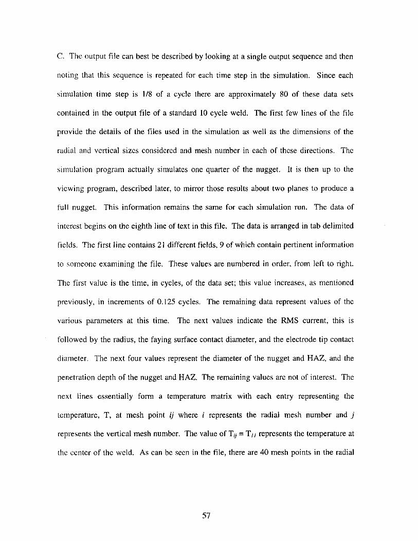
C. The output file can best be described by looking at a single output sequence and then
noting that this sequence is repeated for each time step in the simulation. Since each
simulation time step is 1/8 of a cycle there are approximately 80 of these data sets
contained in the output file of a standard 10 cycle weld. The first few lines of the file
provide the details of the files used in the simulation as well as the dimensions of the
radial and vertical sizes considered and mesh number in each of these directions. The
simulation program actually simulates one quarter of the nugget. It is then up to the
viewing program, described later, to mirror those results about two planes to produce a
full nugget. This information remains the same for each simulation run. The data of
interest begins on the eighth line of text in this file. The data is arranged in tab delimited
fields. The first line contains 21 different fields, 9 of which contain pertinent information
to someone examining the file. These values are numbered in order, from left to right.
The first value is the time, in cycles, of the data set; this value increases, as mentioned
previously, in increments of 0.125 cycles. The remaining data represent values of the
various parameters at this time. The next values indicate the RMS current, this is
followed by the radius, the faying surface contact diameter, and the electrode tip contact
diameter. The next four values represent the diameter of the nugget and HAZ, and the
penetration depth of the nugget and HAZ. The remaining values are not of interest. The
next lines essentially form a temperature matrix with each entry representing the
temperature, T, at mesh point ij where i represents the radial mesh number and j
represents the vertical mesh number. The value of Ti = TI/ represents the temperature at
the center of the weld. As can be seen in the file, there are 40 mesh points in the radial
57
direction and 9 in the vertical direction. This indicates that each dataset will have 9 fields
and 40 lines of data, after this point in the file, data for the next time step is listed.
While it is important to understand the significance of the data contained within
the simulator output file, it is extremely cumbersome to extract any meaningful
information by simply looking at the text. For this reason the Show Out program was
developed. Show Out is a viewing program that provides the user a graphical
representation of the data. Figure 13 shows the user interface of the viewer. With the
program running, the user clicks on the read button to open a simulation output file.
After selecting a file from the dialog box, the program proceeds to read the data from the
file. The program has four main display areas in which it now presents a representation
of that data. The first display consists of two text boxes. These boxes show the molten
nugget diameter and the weld penetration depth at the currently selected cycle time.
Below this, from top to bottom, a graph of welding current, dynamic resistance, weld
center temperature, contact diameter, nugget diameter and penetration depth are shown
vs. time. The top right corner of the screen contains a graphic representation of the
temperature distribution in the weld part. Molten metal is represented in this display by a
pink color. In black and white images, the molten portion can be identified as the solid
light gray area located at the center of the weld. Below this a text box displays each of
the time steps with the corresponding center temperature. The user can scroll through the
text box containing the temperatures to view the center temperature at each simulation
step. The user is also provided with a scroll bar beneath the temperature distribution plot.
This allows the user to update the plot to any of the simulation steps. While the plot of
welding parameters vs. time remains fixed for each file, the values of molten diameter
58

Viewer for simulated nugget formatIon iMolten diameter
Penetratior5.314
Fi-u mm
' U I ime; iU.j( I emp; Ib03.IUTime; 10.75 Temp ; 1576.91Time; 11.125 Temp ; 1549.24
dc Completed to read temperature file;
(C) 2000!
Figure 13 User interface of Simulation Results viewer used to graphically display the
results of finite element simulations of welding conditions.
59
T1

and penetration depth change in synchronization with the changes in the temperature
distribution plot.
A modification was added to the simulation routine in the form of FFT filter in
the Show Wave program. The FFT routine works inline with the Show Wave, however,
upon loading the viewer the user is now required to select a parameter file that defines the
FFT treatment. This file can be found in Appendix C. A check box has been added
similar to the smoothing filter that must be selected before the sample data is loaded.
Figure 14 shows the updated user interface of the program. The standard cutoff
frequency defined in the parameter file for the FFT treatment is 50 kHz and the treatment
is done using 256 data points on every half cycle. To use the FFT treatment, the user is
required to modify the value of the non-dimensional mutual inductance to produce a
waveform with the mutual inductance effects removed to a satisfactory degree. After the
user is satisfied with the results of the treated data they have the option of saving the
treated data for use in the simulation program, or for viewing at another time. It is a
highly recommended practice, which was followed during the course of the study, that
the FFT treated data be saved as a new file and never over the original monitoring data.
Short of repeating the weld under exactly the same conditions and obtaining new
monitoring data, there is no effective way to undo the FFT treatment once it has been
applied. After FFT treatment, the saved data should only be reviewed when the FFT box
is unchecked. It is undesirable to apply a second FFT treatment to the already treated
data. Additionally, it is necessary to set the mutual inductance value to zero since it has
already been accounted for and removed from the data. A non-zero value for mutual
inductance will cause an undesirable shift in the already clean waveform. A similar
60

I .Wavefolm checkei foi monlting data by Lab PCI 200 [iiR] E3Nondimensional
r Noise reduction lI use FFT I nductance Mf~ Auto-set inductance M r inverse 12
C
2 Cycle Rtil: 124 .flL
1 Cycle-- > TimeJ > Time
SkipO; 0, Skip; 6Data:D:\ElLifeA2\ogbe2008.spdt 1=8.883kAData:D:\ElLifeA2\ogbe2008.spdt 1=8.883kAData;D:\ElLifeA2\ogbe2008.spdt 1=8.883kA
a Force curvve InductanceReadlShow, Exit data
Figure 14 User interface of updated Show Wave program using FFT treatment.
61
Brint
I

constraint is imposed when using the FFT treated data as input to the finite element
simulation program. As mentioned in the description of the program, the program's
values of mutual inductance must be set nearly to zero to avoid modifying the cleaned
waveform. The mutual inductance value can not be set exactly to zero, as this will cause
a program error.
3.7 Preparation of Etched Samples
One method to determine the nugget diameter of a spot weld is to cut the welded
material through the center of the weld; the piece is then mounted in epoxy and polished.
The polish specimen can then be etched to reveal the microstructure of the weld. This
etching will show the boundary of the nugget formed during welding as well as the
boundary of the heat affected zone (HAZ). These samples can then be photographed for
further study or have other tests, such as micro hardness of the nugget and HAZ,
performed on them.
The samples to be etched must first be trimmed down to a size that will fit on both
the cutting machines and in the mounting mold. The first trimming step is done on a foot
stamp shearing press. This procedure cuts the welded specimen leaving only the
overlapping section of the metal plates. The rest of the material may be discarded. Once
trimmed down to this smaller length, now approximately 30 mm by 30 mm, the sample is
made thinner by trimming a small section off of either side of the weld using a high speed
cut-off wheel. Figure 15 shows the step by step cutting procedure.
At this point the sample is now ready to be cut to expose the central cross-section
of the weld. This cutting is done on a low-speed saw. The blade used for this procedure
62

100 mm 330 mmm
30 mm (a)
Nugget
0 (b)
Saw BladeWidth
(c)
-4- Viewing Direction--------------- Cuts
Workpiece Boundary
Figure 15 Cutting steps to observe cross section of weld nugget: (a) coarse cut to isolate
nugget, (b) coarse cut to reduce specimen width, (c) fine cut to reveal center cross section
of nugget.
63

is a high concentration diamond coated blade. The blade is aligned such that the center
of the weld is lined up with the inner edge of the blade. Figure 15c shows the proper
alignment of the blade. This ensures that the center of the weld is not removed during the
cutting process. Since some material will also be removed from the cut surface during
the polishing process the edge of the blade may be offset even further to make sure that
the true center of the weld is seen at the final stage of the process. After the specimen has
been cut, it is cleaned thoroughly with soap and warm water and dried. This removes the
oil used in the cutting process from the part. It also removes the contaminants that can
become lodged between the non-welded section of the workpiece during the cutting
process. As the polishing steps progress, a contaminant can cause problems if it is larger
than the polishing grit size used.
The specimen is now ready to be mounted. It is placed in a mounting clip to
ensure that it remains positioned properly as the epoxy is hardening. The desired
mounting position is to have the cut face of the welded part completely horizontal,
parallel to the bottom of the mold. The inside of the mold should be rubbed with a thin
layer of silicon grease to allow easy removal of the sample after the epoxy hardens. The
sample is placed in the mounting cup so that the edge containing the weld is firmly
pressed against the bottom of the cup. The epoxy mixture is made by mixing 15 parts
resin with 1 part hardener. The mixture must be stirred for 3 minutes before use to ensure
homogeneity. When the epoxy is ready, the mold is placed in a vacuum container. The
container is used to draw the epoxy from a holding cup into the mounting cup. The
vacuum also allows most of the air trapped in the epoxy during mixing to reach the
surface and escape before hardening producing a higher quality mounting. Any residual
64

water or air trapped between the welded pieces will also tend to rise to the surface
reducing the effect of the contaminants. Ideally, any gaps between the workpieces would
be filled in with epoxy during the mounting. However, this does not typically happen
because of the viscosity of the epoxy mixture. Therefore, the gap between the
workpieces will continue to be a cause for concern if water or contaminants become
trapped there. Once the mold is filled with epoxy, the epoxy must be allowed to harden
for approximately twenty-four hours at room temperature.
After the epoxy has hardened, the samples may be removed from the mounting
cups. It is necessary to clean the remaining silicon grease off of the samples at this time.
This can wiped off with a dry paper towel. The samples are then polished using a three
step process, prior to which the bottom edges of the epoxy are rounded off to prevent it
from catching the paper. Each step of the process is carried out using an auto-polisher.
The polisher applies a uniform load to each of the samples and allows the user to select
the rotation speed of the polishing disk, the rotation direction of the samples relative to
the disk and the duration of the polishing. In each step, a counter-rotating sample holder
was employed with a load of 30 N on each sample. The first step uses 500 grit sandpaper
at 300 rpm, this step is used to smooth out the cut surface to some degree, but its primary
purpose is to remove the epoxy that may be covering the weld and to expose the metal of
the sample. This step used polishing times in 10 second increments. Since the sample
holder can polish six samples a once, samples that were exposed first were removed so as
not to remove excess metal from the weld. Between each step the samples are rinsed in
water to remove contaminants that could scratch the surface of the metal. The second
step uses 1000 grit paper to further smooth out the specimen. This step is done using as
65

short a polishing time as possible, also in 10 second intervals, to prevent the removal of
excess metal from the specimen. This step is complete when the surface appears to have
a uniform scratch pattern under a microscope. The final step is a polishing step using
4000 grit paper with a rotation speed of 150 rpm. This is done for 30 seconds to ensure a
smooth surface. This longer time is acceptable since this paper removes very little
material and is moving at a slower speed.
After the samples have been polished they are rinsed in warm water and dried.
This drying step is very important as water trapped between the welded parts has a
tendency to seep out over time. When left on the polished or etched surface of the part
this water aids in corrosion causing rust to form on the surface. Once the rust begins to
form, the part must be re-polished. Samples are considered dry after 5 minutes in a hot
air flow and are then ready to be etched. The etching solution is composed of 55 percent
alcohol, 40 percent water, and 5 percent nitric acid. The etching is done in a small glass
dish using between three and five milliliters of solution. For each milliliter of solution
used, one drop of liquid soap is added as an activating agent. The samples are then
placed weld down in the solution and moved slowly for 3 minutes after which they are
removed from the solution and rinsed. The etching is carried out at 20 'C (68 'F). The
samples are then dried with a paper towel and then further dried under forced hot air to
remove any residual moisture. This drying is again critical to prevent rust from forming
on the specimen. For storage the samples are placed in a sealed plastic bag.
The final step in this process is to take a photograph of the etched weld.
Photographing the samples is done on a Leitz microscope using lenses that produce a
photo with lIx magnification. The samples are mounted on the microscope and viewed
66

using the III and IV filters which, on this microscope, produce a light with a green hue.
The instrument is adjusted so that the image on the photo screen is focused. The photo
tray is then inserted into the instrument and the exposure time selected. Exposures of
1/125 s were used for the photographs. Film is inserted into the photo tray and the outer
covering is pulled back out to its edge. This places the film in a position ready for
exposure. The switch on the microscope activates the shutter for the set time. The casing
is then pushed back in and the lever on the photo tray is activated. The entire package,
film and casing, are pulled quickly to the end of the casing. This step allows the
developing chemicals to mix and come in contact with the film. The lever is then
returned to its original position which allows the film and casing to be completely
removed from the photo tray. The film used is Polaroid 54 and is self developing. This
film requires a development time of only twenty seconds. After the picture is removed
from it's casing it can be treated with a polish for preservation.
67
Chapter 4Welding and Simulation Characterization
4.1 Weld Lobe Tests
One of the first requirements in conducting this investigation was to obtain
experimental data identifying the critical welding current for splash and for no-weld. It
was also important to obtain the characteristic form of nugget growth vs. current. This
information was obtained through the weld lobe tests.
Initially, the weld lobe tests were carried out using old electrode tips. These
electrode tips had been used for some time and had therefore experienced a dramatic
shape change in comparison to new tips. Rather than a round contact surface at the end
of the tip, the contact area was distinctly oval shaped. Tests were carried out with these
tips using 1 mm thick galvanealed and organic zinc coated mild steel (SPCC). Weld
lobes were obtained using electrode forces of 100, 200 and 300 daN with a welding time
of 10 cycles. After completing the welding process, the specimens were sheared apart at
the faying surface to reveal the nugget that had been formed. This nugget was then
measured along both the length and the width of the specimen. Figure 16 shows the
results of the weld lobe tests for galvannealed steel specimens using the pneumatic
welding gun with old electrode tips. The figure shows the nugget diameter progression
as welding current is increased. It can be seen from these results that the typical nugget
formed followed the shape of the electrode tip very closely. That is, the nuggets were
oblong in shape with the major axis corresponding to that of the electrode tip. While this
experiment provides a general indication to the critical current conditions the results were
not suitable for further use due to the preexisting deformation of the electrode tips. This
68
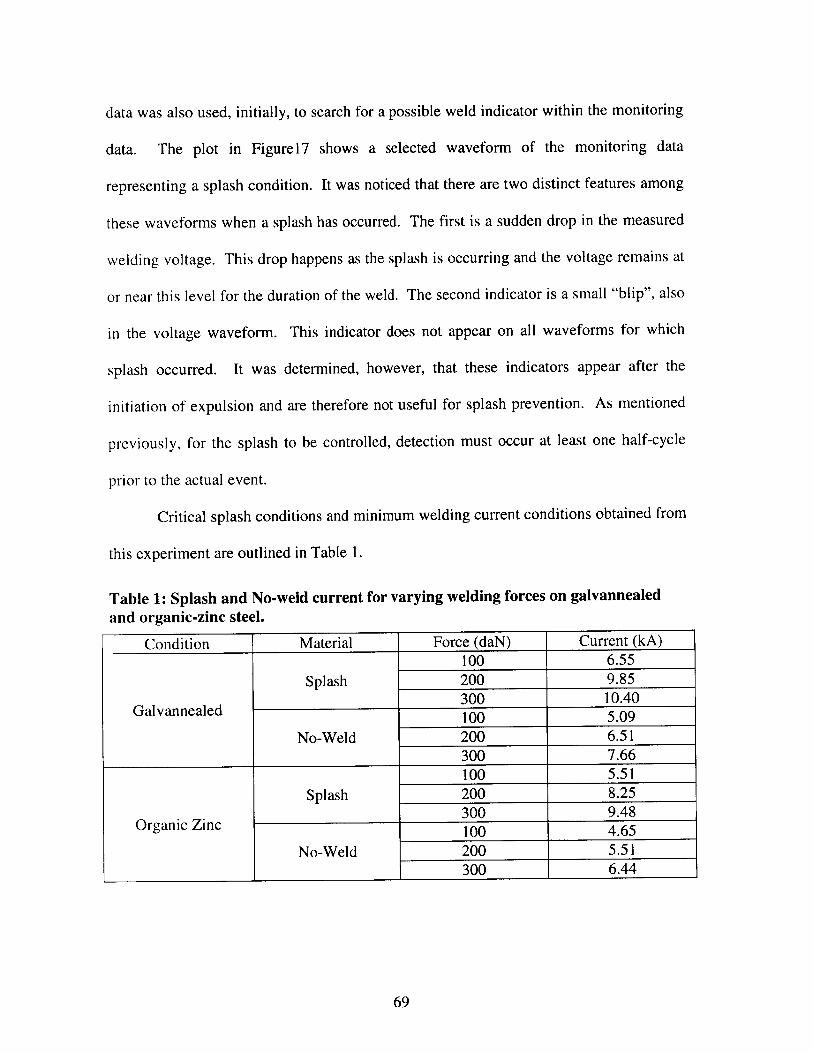
data was also used, initially, to search for a possible weld indicator within the monitoring
data. The plot in Figure17 shows a selected waveform of the monitoring data
representing a splash condition. It was noticed that there are two distinct features among
these waveforms when a splash has occurred. The first is a sudden drop in the measured
welding voltage. This drop happens as the splash is occurring and the voltage remains at
or near this level for the duration of the weld. The second indicator is a small "blip", also
in the voltage waveform. This indicator does not appear on all waveforms for which
splash occurred. It was determined, however, that these indicators appear after the
initiation of expulsion and are therefore not useful for splash prevention. As mentioned
previously, for the splash to be controlled, detection must occur at least one half-cycle
prior to the actual event.
Critical splash conditions and minimum welding current conditions obtained from
this experiment are outlined in Table 1.
Table 1: Splash and No-weld current for varying welding forces on galvannealedand organic-zinc steel.
Condition Material Force (daN) Current (kA)100 6.55
Splash 200 9.85300 10.40
Galvannealed 1050100 5.09No-Weld 200 6.51
300 7.66100 5.51
Splash 200 8.25___________300 9.48
Organic Zinc 300 4.100 4.65No-Weld 200 5.51
300 6.44
69
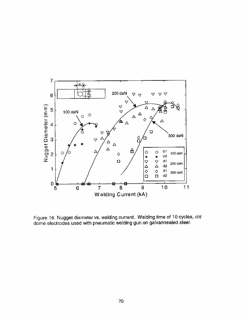
7
6
E5E
40
a 32
z
1
0
200 daN
100 daN
0
- 0
65
1vv7
000
300 daN*0
0 0 dl 100 daNS + d2
0 d2 200 daN
d1 300 daN0 Q d2
7 8 9 10 11
Welding Current (kA)
Figure 16 Nugget diameter vs. welding current. Welding time of 10 cycles, olddome electrodes used with pneumatic welding gun on galvannealed steel.
70
-i 1
0
.di
~
.Aff

4x 10
1
a,
0
0
-1
0 0.05
Figure 17 Waveform of monitoringlobe tests.
0.1Time (s)
0.15
2
1
0
0
-1
Voltage
-2
Current
data taken during splash condition in the weld
71

Figure 18 shows the weld lobe results when organic-zinc coated steel was used as
the test specimens.
These results show that the critical current levels of the organic-zinc coated sheets
were generally significantly lower than those of the galvanealed sheets. However, the
change in current between the splash condition and the no-weld condition are seen to be
nearly the same for both types of materials. This would seem to indicate a constant shift
of the welding range introduced by the difference in material rather than an expansion or
contraction of the welding range.
To obtain data that would better represent the actual tip condition, the electrode
tips were replaced with new ones. With the new tips in place, the weld lobe test was
repeated after conditioning the tips. In this test only coupons of galvanealed steel were
used as specimens. The conditions used were the same, 10 cycles at 100, 200, and 300
daN. When the samples were broken for measurement it was found that the nugget was
no longer of an irregular shape. The nugget again mimicked the shape of the electrode
tip, which was now nearly a true circle. The plots of nugget diameter show that nuggets
measured in either direction were nearly identical. This test was conducted on both the
air gun and servo gun. Figure 19 shows the weld lobe results from the pneumatic
welding gun and Figure 20 shows the results from the servo gun. The critical splash
conditions from each test are outlined in Table 2 below. It should be noted that due to the
discrete setting of the servo force, the actual electrode force used was not exactly 100,
200, and 300 daN. The actual force is listed in Table 2.
72

7
6 k
E5E
+-- 4a)E
CZ3
02Z
1
0
di
L |I
100 daN
0
0-o
*
lI~-HS I 200 daN
0 0
0
300 daN
0 0
o 0 dl100 daN
d v 200 daNA A d2
C C d1 300 daNo Q d2
' ~5 6 7 8 9 10
Welding Current (kA)
Figure 18 Nugget diameter vs. welding current. Weld lobe test results: weldingtime of 10 cycles, old dome electrodes used with pneumatic welding gun onorganic zinc coated steel.
73
-
^ 0
-

8
EE
E
0
0J)
z
7-
6
5
4
3
2
1
0
d1
100 daNd
300 daN
0 0o o dl 100 daN. +d2
dl 200 daNA A d2
o d2
6 7 8 9 10 11 12Welding Current (kA)
Figure 19 Nugget diameter vs. welding current. Weld lobe test results: weldingtime of 10 cycles, new dome electrodes used with pneumatic welding gun ongalvannealed steel.
74

6 7Welding
8Current
200 daN
300 daN
0 0 dl 100 daNS+ d2
dl 200 daNAAd2
S(1 300 daNo [ d2
109(kA)
Figure 20 Nugget diameter vs. welding current. Weld lobe test results: weldingtime of 10 cycles, new dome electrodes used with servo welding gun ongalvannealed steel.
75
7
6-
5 -
4-
3F
.
100 daNEE
E
0)z
1
05 11
2 V

Table 2: Splash and No Weld currents for varying welding forces on air and servowelding guns.
Welding Machine Condition Force (daN) Current (kA)100 6.78
Splash 200 8.12
AirGun 300 11.31100 4.97
No-Weld 200 5.40300 6.3895 7.08
Splash 205 9.08308 10.31
Servo Gun9547N-ed95 4.70
No-Weld 205 6.05308 5.98
There are minor differences between the results from each machine; however,
neither machine seems to produce consistently higher or lower current values. It is
believed that the difference in actual welding forces between the machines is responsible
for the observed differences. It is also believed that the difference in impact speeds of the
electrode tips may contribute to the variation. The servo gun has a higher impact speed
when the specimens are clamped between the tips. This is also thought to cause greater
wear and deformation of the electrode tip.
It was also necessary to conduct experimental welds using a constant current and
varying the welding time used. In this test, the objective was to capture the nugget
formation at a particular current every two cycles. In conducting this test it was assumed
that the variations seen in the actual welding current were not significant enough to effect
the nugget diameter. Likewise, the electrode force was assumed to be constant for each
weld.
This test was performed in conjunction with the weld lobe tests. It was performed
after the completion of the weld lobe for a given electrode force. The weld lobe data was
76

used to select a welding current that fell within the range of acceptable nugget sizes and
below the splash condition for a 10-cycle weld. This test was performed on galvanealed
steel sheets with both the air and servo guns. This data was saved and used for further
verification of the simulation program. The results will therefore held and reported in
Chapter 5 to improve understanding of their meaning.
4.2 Electrode Life Tests
As described in the methods section, the electrode life test sought to characterize
the nugget progression under a fixed welding condition over a large number of welds.
The test was completed when a nugget was produced that fell below the minimum
acceptable nugget diameter. After completing the test, a representative sample was taken
from each group of one hundred welds and broken on a tensile machine. This was done
not only to identify the ultimate tensile strength of the weld formed, but also to expose
the weld center so that its diameter could be measured.
It was found that as the number of welds produced increased, the nugget diameter
decreased. As is expected, a decrease in nugget diameter also leads to a structurally
weaker weld. The weld lobes conducted each one-thousand welds are shown in Figure
21. The nugget diameter and tensile forces of the specimens are shown vs. weld number
in Figure 22. The relationship between weld diameter and tensile strength was found to
be nearly constant, this is shown in Figure 23. This is as expected since the strength of
the nugget is dependent on the surface area of the nugget cylinder that is a linear function
of nugget diameter. The data obtained from the electrode life test would be used later in
the investigation to verify the results obtained from the finite element simulator. Once
77
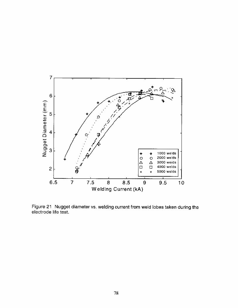
7
6-
EE
-)
E
TO -00
0)
* * 1000 weldsz- 0 2000 weldsA A 3000 welds
2 5 4000 weldsx x 5000 welds
I II I I I
6.5 7 7.5 8 8.5 9 9.5 10Welding Current (kA)
Figure 21 Nugget diameter vs. welding current from weld lobes taken during theelectrode life test.
78
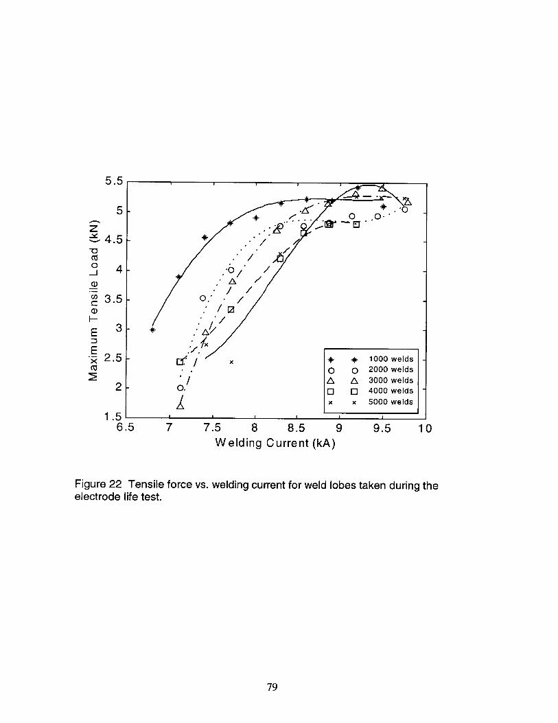
5.5
5 <+~* < 0 0
4 5 - ET--
4.5 . +
A /-j 4 -. 10/3.5 - 0.,
I- /
E 3 -
-2.5 + + 1000 welds -
0 0 2000 weldsA A 3000 welds
2 0. E] [ 4000 welds -x x 5000 welds
1.56.5 7 7.5 8 8.5 9 9.5 10
Welding Current (kA)
Figure 22 Tensile force vs. welding current for weld lobes taken during theelectrode life test.
79
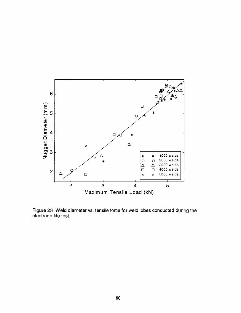
E 006 - -
E_ 5 - + -
00C)
E
A+ + 1000 weldsZ x *o o 2000 weldsA A 3000 weldso 2 4000 welds
Al x x 5000 welds
2 3 4 5Maximum Tensile Load (kN)
Figure 23 Weld diameter vs. tensile force for weld lobes conducted during theelectrode life test.
80

the nugget pattern of the electrode life test was observed to coincide with what had been
expected, the data would prove useful for this purpose.
The weld lobes conducted throughout the electrode life test would be used for two
purposes. The first was to identify how the weld lobe changes over time. This is
important because it represents the variation in the critical splash condition with weld
number. One would be wrong to assume that the critical splash current remains constant.
Instead, it is widely recognized that the splash condition decreases, while at the same
time the current needed to form a minimally acceptable nugget increases. Figure 24
shows the variation in these values as weld number increases. As the electrode tips wear
this pattern brings the two current levels close to each other. It is in the time when these
current levels are nearly the same, that the control process is most important.
Additionally, Figure 25 depicts the current level difference between acceptable nugget
formation and the splash condition. It can be easily seen from this figure that the two
currents tend to merge to a common value making selecting a good welding current
increasingly difficult, if no control procedures are implemented. A second function of
the weld lobe test was to provide experimental data with which to verify the simulation
program. These weld lobes provide the opportunity to check the sensitivity of such
program parameters as tip resistance and tip shape. Since both change over the course of
the test, a simulation program that could accurately predict nugget diameter, without
modifications needed in these values, would be considered insensitive to these values and
would be an extremely attractive model.
During the course of the test, an impression of each of the electrode tips was taken
every two hundred welds. These impressions show that the upper tip experienced a much
81
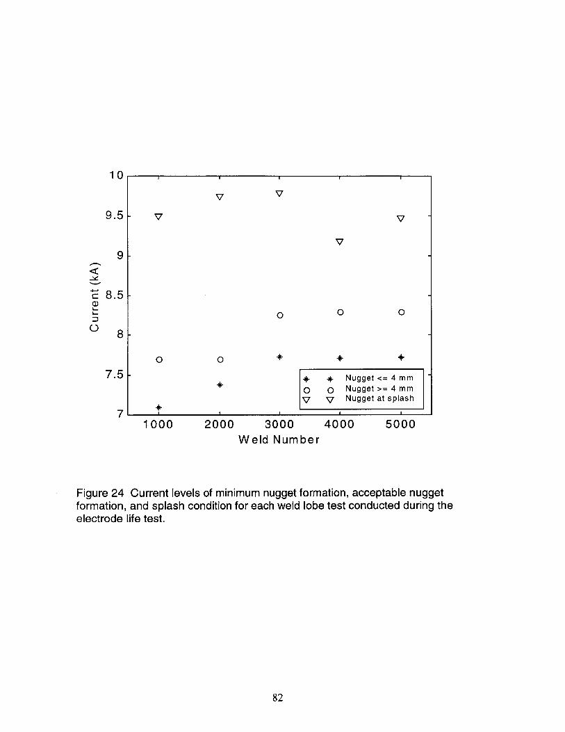
10
9.5
9
8.5
8
7.5
7
,V
0 0
o a + + *
*+ + Nugget <= 4 mma a Nugget >= 4 mm
V V Nugget at splash
1000 2000 3000 4000 5000Weld Number
Figure 24 Current levels of minimum nugget formation, acceptable nuggetformation, and splash condition for each weld lobe test conducted during theelectrode life test.
82
C)

2.5
2-
C 1.5-
C
0.5 -
01000 2000 3000 4000 5000
Weld Number
Figure 25 Difference between critical nugget formation current and splashcondition current over the course of the electrode life test
83
greater change than the lower tip. This can be seen in the progression shown in Figure
26. The lower tip is seen to remain nearly constant in size and shape; however, the upper
tip contact area clearly becomes larger over the course of the test. These results are
believed to be a result of the material in contact with each of the tips. The lower tip is
always in contact with bare steel; this is because there is no coating placed on the bottom
of the welded specimens. The upper tip, however, is always in contact with the organic
zinc coating placed on the opposing surface of the specimens. It can therefore, be
concluded, using the bare steel as a baseline, that the zinc coating contributes to the
increased deformation of the electrode tip. The cause of this is the chemical reaction
between the copper of the electrode tip and the zinc coating described in the introduction.
A plot of tip diameter vs. weld number is shown in Figure 26. The plot clearly shows
that the upper tip diameter grows much more rapidly than the lower tip.
To generate further data for use in verifying the simulator program, two of the
weld lobes of the electrodes were cut, polished, and etched. The samples were then
photographed at a magnification power of 10. The photographs could then be used to
detect the nugget diameter as well as the boundary of the heat affected zone, and the
penetration depth of the nugget. These last two values can only be obtained by this
method and not by using the tensile test method. The standard microstructure of mild
steel as seen at this magnification is a very fine-grained structure. At such a low
magnification it appears as a fine, uniform texture on the surface of the material. The
heat affected zone and nugget, in contrast, have much coarser microstructures. They
appear to have a dendrite form with sharp contrast between the grain boundaries. The
nugget boundary actually appears as a thin line through the microstructure. Figure 27
84

7
6.5
EE
E
azQ-
61
5.5
51
4.5
AA AAAAAAA
- *+AAA.+++++
Upper TipA A Lower Tip
0 1000 2000 3000 4000 5000Weld Number
Figure 26 Tip diameter vs. weld number for electrode life test.
85

shows the growth of the nugget and heat affected zone for increasing weld time for the
same welding conditions. All welds were conducted using a welding force of 200 daN
and a welding current of 7.40 kA on the pneumatic welding gun. The figures show
nugget size starting from Figure 27a at 8 cycles and increasing to 27c after 12 cycles,
where I cycle is equal to 1/60 seconds.
86
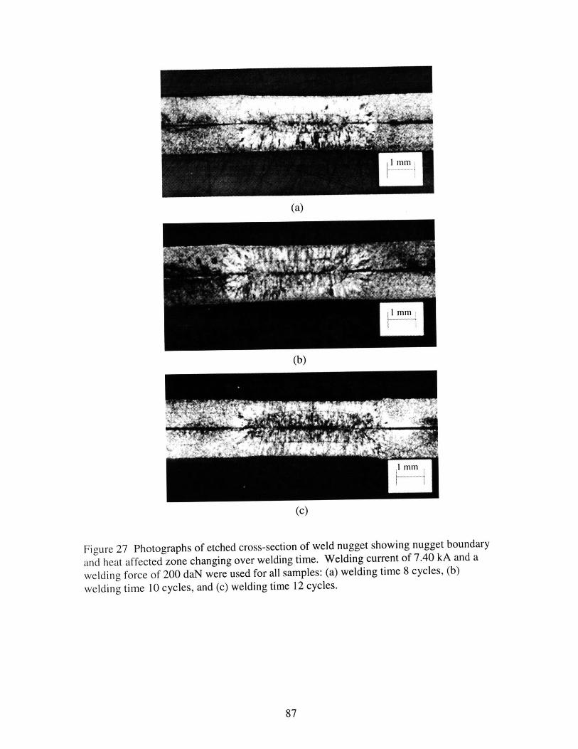
(a)
(b)
(c)
Figure 27 Photographs of etched cross-section of weld nugget showing nugget boundary
and heat affected zone changing over welding time. Welding current of 7.40 kA and a
welding force of 200 daN were used for all samples: (a) welding time 8 cycles, (b)
welding time 10 cycles, and (c) welding time 12 cycles.
87

Chapter 5Simulation and Temperature
Estimation
5.1 Finite Element Simulations
One of the major steps of this investigation was the verification of the finite
element simulation program. This process involved two major tasks. The first was to
identify those simulation parameters that the simulation results were insensitive to
changes. This was carried out by considering a small number of welds and making
similar variations to welding parameters in each. The results were then compared to each
other and to the experimental data from the weld. Once the insensitive parameters were
identified, the second step could proceed. This consisted of making simulations of a
large number of welds. In this process, the insensitive parameters were left as constants
while the sensitive parameters were modified. This served to further verify that the
parameters chosen in the first part were indeed insensitive as well as to determine which
values of the sensitive parameters are best suited to the simulation under different
conditions. The final step of the simulator verification process came with the comparison
of the use of FFT treated data as input as compared to using the original monitoring data.
As described above, the initial verification of the simulator involved the
identification of sensitive and insensitive parameters. Several parameters were
immediately identified as requiring verification. These included the value of the
resistance of the electrode tip (Rip), the resistivity (p) of the specimen, the difference in
contact diameter (de) and electrode tip diameter (de), and in later tests, the value chosen
for the mutual inductance.
88
The first values considered were those pertaining to resistance, Riip and p. These
values were varied independently. Variations of ten percent were imposed on each value
and the results were compared. The results show that for a large variation in either of
these parameters the predicted weld nugget variation was much smaller. The effects of
change in the resistivity were found to be negligible; therefore, future tests were
conducted using a constant value for resistivity. Changes in the value of Rtip, however,
were seen to have a greater impact on the valued of the predicted nugget size. Since
changes in tip resistance itself can be considered negligible, except in the case of large
weld numbers, the tip resistance was only modified when conducting experiments on the
electrode life test data. For this data a linear approximation of tip resistance was made as
a function of weld number. This approximation was made from actual tip resistance data
taken during the test. During the simulation run the tip resistance value was recalculated
for changes in weld number of 1000 or more and was assumed to be constant for all
welds over that range.
Next, consideration was given to the value of the contact diameter and electrode
tip diameter. It was found that the critical value to consider in this case is not either of
the individual values, but rather the difference between the two values, dc-de. The initial
formulation of this parameter is given as:
dc -de =ah (4)
where d, is the workpiece contact diameter, de is the contact area of the electrode-
workpiece interface, h is the workpiece thickness, and a is a material dependent constant.
89

That is, the difference is proportional to a constant times the thickness of the
material being welded, measured in mm. The constant, a, varies depending on the
coating of the material being used. The initial values of this constant are shown for each
material considered in Table 3.
Table 3: Values of a for common steels.
Material Values of a
Galvanealed 0.7-0.8
Bare Steel 0.5-0.6
Organic Zinc Coated 0.6-0.7
When tests were run using modified values of this parameter it was found that the
predicted values of the nugget diameter varied dramatically. The parameter dc-de was
immediately identified as a sensitive parameter and could not be considered constant for
each weld. This parameter of interest will be known as the contact diameter difference,
A. Once this was determined it remained to be seen if a value could be found that would
accurately predict the nugget diameter. This would mean that rather than varying with
each weld, the value of Ac would depend only on the material being welded. Due to the
sensitivity of the simulation on A, choosing the appropriate value would be the most
difficult part.
The final parameter of concern was the value of the mutual inductance that the
simulator applied to the monitoring data. In later experiments the monitoring data had
been treated with a FFT routine that smoothed the data. In processing the data on the
modified Show Wave, it was also possible to remove the mutual inductance during the
90
treatment. This data was saved and used as input to the simulation program. The mutual
inductance of the simulator had to be modified to insure the effect of the mutual
inductance was not removed from the data twice. However, the calculations involving
the mutual inductance in the simulator required that it have a non-zero value. As a first
attempt the mutual inductance values were simply set to very low values. Initial results
showed that the results matched up well with those obtained before the treatment. It now
remained to be seen how variations in the values would effect the output.
It can be clearly seen from this data that, large changes in mutual inductance do
not have any meaningful impact on the predicted nugget diameter. This value was found
to be insensitive and could be considered to alternate between two constants, one for
untreated data and the second for treated data. The actual results of the simulations using
FFT treated data can be seen in the following sections.
The results from the simulations on untreated monitoring data immediately
showed a very good accuracy for predicting nugget diameter. These simulations were
run on the weld lobes of both the air gun and the servo gun as well as the weld lobes
conducted throughout the electrode life test using organic zinc coated sheets. In the
simulations of the standard weld lobes, the value of tip resistance was fixed by the
average value obtained from tests of a thin copper sheet placed between the electrode
tips. The value for these tests was set at 25 g. For the electrode life test, the tip
resistance was determined by measuring the tip resistance every 1000 welds throughout
the test. An equation was fit to the data obtained to give the resistance at a given point in
the test. The resistance as a function of weld number is described as:
Rtp = 0.002127N+20 (5)
91

where Rip is the tip resistance and N is the weld number.
The tip resistance was found to vary between 20 p.Q and 30 pQ. The resistivity of
the material was fixed as a linear equation in the matconwla.dat file. The resistivity was
given as a function of temperature that the simulation would calculate for each mesh
point of the sample. The equation is:
p = AT2+BT+C (6)
where T is the mesh point temperature in 'C.
In this simulation values chosen were A=10.56 x10⁻⁵ gL.cm/C 2 , B=3.575 x 10-
p2.cm/C, and C=16.0 pQ.cm. The value of the mutual inductance, AMIND1 and
AMIND2 in the simulation input, was not considered until the FFT treatment was applied
to the data. For this simulation process the values used were AMIND1=0.2 and
AMIND2=0.05. The final value was A,, which had been determined to be the sensitive
parameter. It was this value that was varied over successive simulations to determine the
best value to use for accurate nugget diameter prediction. Since the crucial factor is the
difference, A,, rather than the absolute value of either d, or de, the value of de was set to a
fixed 3.5 mm. The value of d, was varied to produce the resulting change in Ac.
The first simulations conducted were carried out on data from the electrode life
test. These tests sought to verify the use of equation 5 for electrode tip resistance
described above. As the data from the results shows, the resistance produced results that
accurately reflected the measured nugget diameter. All of these tests were conducted
using a constant resistivity and a Ac value of 0.7 mm. When variations were made to the
tip resistance and the samples rerun, the resulting change in predicted nugget diameter
was very small compared to the change imposed on the tip resistance. This not only
92

substantiated the consideration of the tip resistance as an insensitive parameter, but also
showed that the proposed tip resistance equation would be sufficient to obtain accurate
simulation results.
Initial variations in A, were carried out in very small increments. The original
changes were found to produce nearly identical results. The changes in these values had
to be increased until significant changes in nugget diameter were observed. This
occurred with changes in the Ac value of 0.1 mm or greater. The range first considered
was from Ac = 0.9 mm to A, = 0.5 mm with the initial value chosen at 0.7 mm. Data from
these initial calculations are shown in graphical form in Figure 28. It was possible to
make two conclusions from this initial run. First, the behavior of the nugget diameter in
relation to the A, value was that nugget diameter increased as A, decreased and a
corresponding increase in Ac would trigger a decrease in predicted nugget diameter.
Second, Ac values of 0.7 mm and above produced predicted nugget diameters that were
too small. The errors of these simulations typically exceeded 20-30% and were well
above the ±0.05 mm range that was targeted for the simulations. The results from a set of
simulations using variations in A, from 0.5 to 0.9 mm is in Table 4:
Table 4: Simulation results for variations in A,
Ac values (mm)Sample Number Exp. Result 0.5 0.6 0.7 0.8 0.9
1004 6.17 6.20 6.20 6.07 5.81 5.801007 6.32 6.55 6.22 6.20 5.97 5.841008 6.54 6.55 6.55 6.20 5.95 5.871011 5.75 5.80 5.80 5.71 5.49 5.40
From the simulation results it was possible to narrow down the range of A, values
for which to conduct simulations. From Figure 28 it is clear that the two best choices for
93

6.5EE
c
Cz
5.5 0
o o 0.5A A 0.6
O 0.7x x 0.80 0 0.9
8.5 9 9.5Welding Current (kA)
Figure 28 Predicted nugget diameters as a function of Ac in the simulationprogram.
94
-R
I
'-
A, are 0.6 and 0.5 mm. Once the parameter ranges had been narrowed down, additional
simulations were run on a wide variety of monitoring data. This data included the
original weld lobe tests and weld lobes conducted throughout the electrode life test. The
optimal value of A, was found to be different for each of the materials considered. While
a A, value of 0.5 mm produces the best results for the galvanealed sheets, the organic zinc
coated sheets are better simulated using a A, value of 0.6 mm. The results show that for
the optimal setting of A, the error between the predicted nugget diameter and the
experimental nugget diameter are less than 10% and more importantly, less than ±0.1 mm
absolute difference.
5.2 FFT Treated Simulations
When an FFT treatment was applied to the same monitoring data it was first
necessary to determine as suitable value of the mutual inductance, M, to be removed from
the data during treatment. This was done manually by choosing a value for the non-
dimensional mutual inductance in the Show Wave program and observing the effect it
had on the voltage vs. current (V-I) curve. The ideal value of M would produce a V-I
curve that was entirely linear. A poor value of M would produce a very rounded V-I
curve. Examples of each of these are shown in Figure 29 a and b. The fact that this value
of M had to be applied over each cycle also made the process more difficult as the value
varied slightly between cycles and a truly linear curve was nearly impossible to obtain
with a single value of M. The final choice of M also varied by material type. For the
galvanealed coated steel an M value of 16 was chosen which corresponded to an actual
inductance of 0.14 gH. For the organic zinc coated steel, a value of 12 was chosen for
95

0 WavefoFM checker for montoing data b Lab PCI200Nondfmnsional
F Noise reduction P' use FFT
F Auto-set inductance M OnversePrw"it CvV
2 Cycle Rtip:1112.4 uOhmr Show dRi'dt tw;J h Cyc
F dR/dt Mode I; 1830
fv Magnify time scale p 194 daNCl 2000-2001 KM 0.3b
1 ---> TimeCycle ~ I 1Eit
Inductancenfco
SkipO;0, Skip;6Data;D:\ELifeA2\ogbe2OO8.spdt 1-8.883kADataD:\ELifeA2\ogbe2OO8.spdt 1-8.883kAData;D:\ELifeA2\ogbe2OO8.spdt I-8.883kA
r Show Force curve j sayer smoothingadflJ Ej a
Force curve
Skip number-5
(a)
04 - Iae(F chce IO moton data by La xI0Nolrdimnionalr Noise reduction ruse FFT In.uctam m -
r Auto-set inductance invese 35PoLarit Lor I
v
. V .. .....
Htap:19587 unhm
tw; rI ; r8883
3 Cycler Show dR/dtF dR /dt Mode
lV Magnify time sc(Cl 2000-2001 KM
Data;D:\ELifeA2\ogbe2008.spdt l-8.883kAData;D:EILifeA2\ogbe20O8.spdt l-8.883kAData:D:\EILifeA2\ogbe2008.spdt I-8.883kAData;WD:ELfeA2\ogbe2008.spdt l=8.883kA
Exit d~ atakA
,P r9_4 daN
(b)
Figure 29 Monitoring waveform comparison of data using (a) properly chosen value of
mutual inductance and (b) poorly chosen value of mutual inductance.
96
V
/
} /
-UA
J'Inductance
F 24 uH
I'd

M, corresponding to 0.10 gH. A second method of verifying a good value of the mutual
inductance was to look at the voltage and current waveforms vs. time. In this plot, a
satisfactory M value would make the peaks of the voltage and current curves line up. An
unsatisfactory value would impose a large phase shift between the two curves. This
phase shift can be seen in the waveform portion of Figure 29 b. The plots in Figure 29 a
and b show the results of treating data with the values chosen above. After an acceptable
mutual inductance value had been chosen, the FFT treatment could be applied. The FFT
treatment serves to smooth the voltage and current waveforms by eliminating noise
greater than a certain frequency. As mentioned in the methods section, the cutoff
frequency for this FFT treatment was 50 kHz. Figure 30a shows the results of the FFT
treated data. Figure 30b shows the untreated form of the same data file for comparison. I
need to wrap this
After treatment of the data, the simulator could be used to obtain a predicted
nugget diameter. The simulator was run in the same manner with the FFT treated data as
it was for the original monitoring data. The major parameter change came in the values
of mutual inductance for the simulator. These values, AMINDi and AMIND2, were set
at 0.001 and 0.0001, respectively. The parameters AMINDI and AMIND2 serve as the
simulation program mutual inductance values. The parameters are used to eliminate the
effect of mutual inductance on the voltage waveform during the simulation. However,
during the treatment by the Show Wave program, the mutual inductance effect is
removed. It is then necessary to set the simulator values very near zero to prevent a
double treatment of the data. A zero value would result in a program error so values were
chosen that were two orders of magnitude lower than the original values. The
97

Wavefom checkew fOF montoting data by Lab PCI12
rr
Noise reduotion M e FF
6Au-set inhCWante 4, nnyerse 1~~2Pnanwit f(W-
V
~---*1
9
2 CycleF Show dR/dtr dR/dt Mode
W Magnify time scICl 2000-2001 KM (
Rtip- 112.4 u)hM
tw 0I , 8.883 kA~
P j194 daN
> TmeCycle
jSSkipO;0, Skip;6Data;D:\ELifA2\ogbe2008.spdt 1-8.883kAData;D:\EL 2\ogbe2008.spdt I=8.883kAData;D:\ELifeA2\ogbe2008.spdt 1-8.883kA
rSho Frce cuive ' Inductance
smolo 6--9Force edata
Skip number-5
(a)
' Auto-set indL
v
4-.
2r CycteShow dR/ddR/dt Mode
lv Magnify time scaleCl 2000-2001 KM O.3b
map 11o.34 uOhnm
I ; 18-883CAckA
P 1194 daN
I-!
Data;D:\Eife&A2\ogbe2008.spdt 1-8.883kADataD:\ELifeA2\ogbe208.spdt I-8883kAData;D:\ELii42\ogbe200.spf I-8.883kAData;DAELieA2\ogbe208.spdt 1-8.883kA
r Sk w Force Irnductance
Skip rumber-5
98
(b)
Figure 30 Monitoring waveform comparison with (a) FFT treated data and (b) non-FFT
treated data.
.-> i
I .-
21

simulations were again run for values of A ranging from 0.5 to 0.7 mm in 0.1 mm
increments. The first comparisons were made with the results from the simulation using
AC = 0.7 mm. These results showed that the predicted nugget diameter obtained from the
treated data was generally lower than that obtained from the untreated data. Based on the
prior conclusion that 0.7 mm was the maximum acceptable value of AC, it was determined
that larger values would not have to be simulated for the treated data either. After
comparing the results obtained from the simulations on both electrode life test data and
weld lobe data, it was clear that the optimal value for A, for treated data was 0.6 mm for
data from organic zinc sheets and 0.5 mm for data from galvanealed sheets. These values
correspond to the optimal values obtained for the untreated data. Figure 31 shows a
comparison of simulations with FFT and non-FFT treated data for three different values
of Ac. The figure shows that in each case, the simulation results for the using FFT
treatment are less accurate than the untreated data. One benefit of applying the FFT
treatment is that the treatment will often produce usable data from data that was
previously incapable of running to completion on the simulator. In the case of extremely
noisy data, often a simulation using the untreated data would cause the simulator to
generate an error and exit after only a few cycles of simulation. However, with the noise
removed by the FFT treatment, the new data file becomes a valid input to the simulation
program and runs successfully to completion. This provides the user an incentive to
apply the FFT treatment before simulation.
Further simulations were carried out for the weld lobes of galvannealed steel for
varying welding forces. A constant Ac value of 0.5 mm was used for all of the
simulations with no FFT treatment. Figure 32 shows the comparison of the simulated
99

* * Exp. Result
A A 0.5
V V 0.5 FFT
o O 0.60 0 0.6 FFT
> > 0.7c 0.7 FFT
9Welding Current (kA)
9.5
Figure 31 Simulation results comparing FFT treatment to untreated data usingthree different values of Ac.
100
7
EE
E
EC0)
6.5 -
6 -
8.5
Splash"
-A
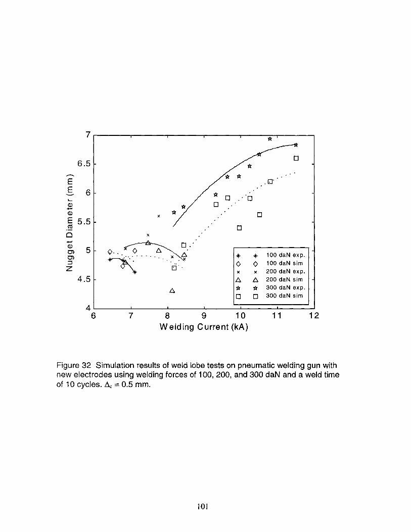
I I I I * I
0
x
4. * 100 daN exp.O Q 100 daN simx x 200 daN exp.A A 200 daN sim* * 300 daN exp.0 0 300 daN sim
8Welding
9Current
1110(kA)
Figure 32 Simulation results of weldnew electrodes using welding forcesof 10 cycles. Ac = 0.5 mm.
lobe tests on pneumatic welding gun withof 100, 200, and 300 daN and a weld time
101
7
6.5 -
6
5.5
EE
CDEC
5 1-
4.5 k
46 7 12
I I I

results and the experimental data for weld lobes of 100, 200, and 300 daN welding forces.
The figure shows that the simulator is effective in predicting the actual nugget diameter.
However, it was also found that the simulation produces the best results for the 200 daN
weld lobe. The results are somewhat less accurate for the 100 and 300 daN simulations.
Simulations for the weld lobes in the electrode life test produced similar results.
Figure 33 shows a comparison of simulation results using both 0.6 and 0.7 mm for Ac.
The figure shows that 0.6 mm is the better choice for Ac which agrees with the results
obtained previously for organic-zinc coated steel. The results for AC = 0.6 mm are very
close to the experimental values. Figure 34 shows the simulated results for the weld lobe
after 2000 welds. The simulation was carried out for a Ac value of 0.6 mm only. Again
the results are found to be within the desired range from the experimental data.
5.3 Temperature Field Estimation
After examining results from the finite element simulation program and verifying
their accuracy a new welding model was considered. This model consisted of the heat
balance model of the weld specimen and is described in the background section. The
heat balance results were compared against experimental results and simulation results to
test its validity.
Heat balance results were obtained from a modified version of the Show Wave
program. Modifications were made to the viewer which provide a mean nugget
temperature estimation for each half cycle of the weld. When this process is carried out
for welding data from an entire weld lobe, the maximum mean temperature calculated
can be seen to have a very close correlation to the measured welding diameter.
102
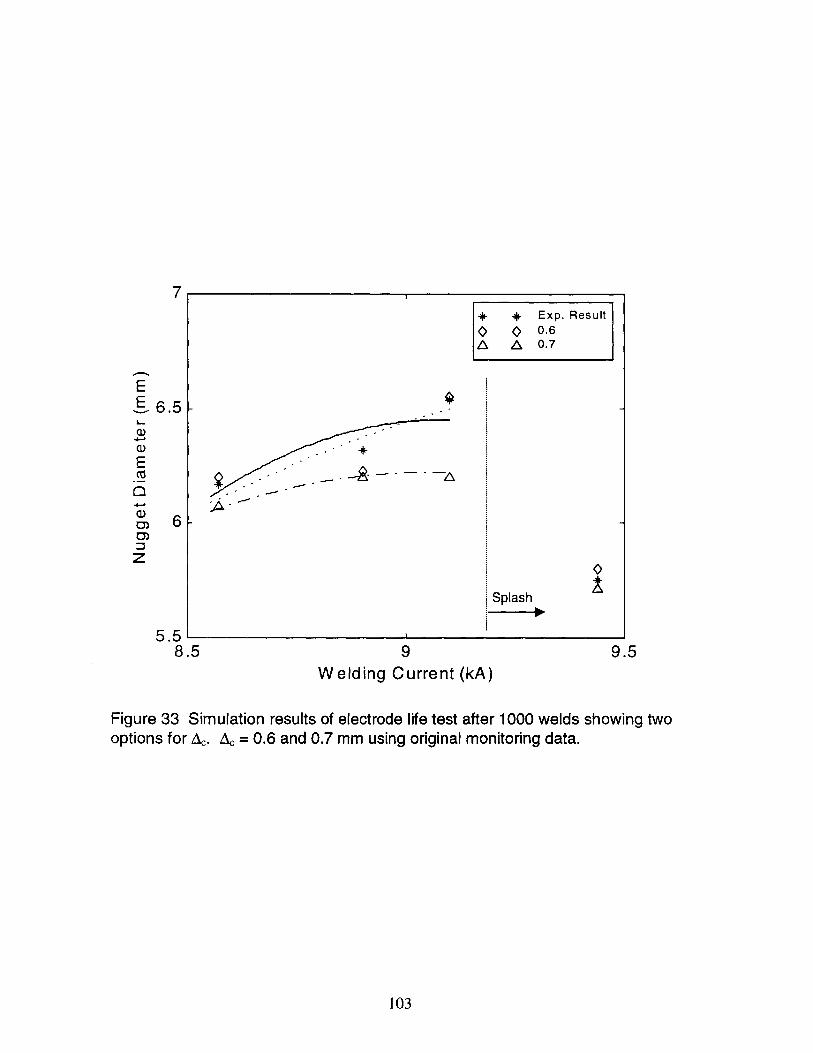
6 -
5.518.
7
EE
E
0)0)
z
6.51-
*0
SplashA
Figure 33 Simulation results of electrode life test after 1000 welds showing twooptions for Ac. Ac = 0.6 and 0.7 mm using original monitoring data.
103
5 9Welding Current (kA)
9.5
* + Exp. Result
0 0 0.6A A 0.7

7
6.5 1
EE
E
Cz
6 1-
5.51.
5 k
4.5
A
Exp. Result
8 8.5 9 9.5 10Welding Current (kA)
Figure 34 Simulation results showing selected Ac value after 2000 welds ofelectrode life test. Ac = 0.6 mm.
104

Figure 35 shows the plot of nugget diameter vs. maximum mean nugget
temperature. Using the results from the simulation program, two additional features of
the heat balance model can be checked. First, the model can be compared to the
temperature distribution predicted by the simulation. However, the simulation predicts a
range of temperature distributed over a mesh, while the heat balance model only predicts
a mean temperature. Therefore, a direct comparison is possible only for temperatures
before the melting condition occurs. It is being investigated whether a mean temperature
reading could be applied to the simulation, allowing further comparison after melting.
Second, since the simulation results have already been verified against experimental data,
the simulator can be used to check additional weld lobes without the need to actually
obtain experimental nugget diameters.
From this comparison to experimental data, it is easy to see that there is a very
close relation between nugget diameter and mean temperature as estimated by this model.
Further, it can be seen that a critical temperature value presents itself where, above this
temperature, a splash will occur. This is seen in comparison to several weld lobe
conditions. The benefit of this model is the relatively short calculation time needed to
obtain the temperature, especially when compared to the simulation program considered
previously. This improvement in calculation time is enough to make it a viable candidate
for use in a real time control system. An added benefit of this system is the reduction in
input values. As shown in the equation above and the derivation in the background
section, this system only requires that the welding current and voltage be measured. The
calculation is independent of tip resistance, material resistivity, and A.
105

7
El 0
6-
E
--
E 0
S3-
0 0 after 1000 welds
j jj 20002 -A 3000
0 0 4000V V 5000
11000 1200 1400 1600 1800
Temperature (C)
Figure 35 Nugget diameter vs. maximum mean temperature as method ofcharacterizing nugget formation.
106

Chapter 6Discussion
6.1 Weld Lobe test results
After examining the results of the weld lobe tests, it became clear that there were
certain underlying relationships between the controlled variables, electrode force,
welding current, and welding time, and the occurrence of a splash. Since the welding
process is controlled by adjusting the welding current, the observations are related by the
change seen in the current level required to produce a splash condition.
It was found that as the electrode force is increased, the current at which
expulsion occurs is increased. This is due to two factors. First the increased deformation
of the electrode tips caused by the increased force causes the contact area of the tips and
the test coupon to also increase. This is transmitted through the test coupon to the faying
surface where the contact area between coupons is greater. Since this contact area acts as
a containment zone for the molten metal during welding, the increased area allows the
weld nugget to grow to a larger size without expulsion occurring. Second, the larger
contact area causes a corresponding drop in current density resulting in less heat
generation.
In contrast, as the electrodes wear, the critical splash current begins to decrease.
At the same time, the minimum current required to produce a satisfactory weld increases.
Over a prolonged usage time, the two currents will begin to converge. This convergence
must be effectively handled in the welding controller design to ensure effective control
over the entire electrode life.
107

6.2 Splash Indications
By examining the output from the welding monitoring program and the weld
simulator, it was possible to identify specific portions of various waveforms that were
indicative of a splash occurrence. These indicators were identified by examining
differences between data of known splash conditions and those of acceptable welds.
The indication of a splash occurrence can best be seen in the graphical
representation of the monitoring data taken during the welding cycle. When the voltage
and current waveforms are plotted versus time the change caused by the splash condition
becomes apparent. The current waveform is seen to remain nearly constant, except for a
half-cycle start-up and shut-down. This is expected since the welding controller is set
and controlled by specifying a constant current output. However, the voltage waveform
varies as the resistance of the weld specimen changes. It is the voltage waveform in
which the splash condition can most readily be observed. The splash is typically
characterized by a sudden drop in the voltage waveform. The underlying cause of this is
the reduced resistance that is introduced into the welding loop when the molten metal is
expelled from the weld. An alternate method of describing this indicator would be to
consider the dynamic resistance of the weld part. That is, the time-varying resistance,
calculated from the measured current and voltage. This value is valid while the current is
above thirty percent of its peak value, and therefore only calculated during these intervals
of the welding cycle. For typical welding conditions, the dynamic resistance is seen to
remain essentially constant over any single half cycle for which it is calculated. Over the
course of the entire weld cycle, the dynamic resistance would be expected to increase
slightly as the resistivity of the material will increase as the material temperature is
108

increased. When a splash condition is examined, the dynamic resistance will be seen to
drop off sharply over the course of one or two half cycles. This drop-off is the
demarcation of the splash occurrence.
There are several important points to consider regarding this particular splash
indication method. First, the indicator, in both resistance and voltage waveforms can
only be seen after the actual splash has occurred. Therefore, these indications can only
be used to identify the presence of a splash. The indicators can not be used to predict or
control the splash as there is no precursory warning of the impending expulsion.
Additionally, while these particular indicators are appreciable in most cases, there are
several observed splash conditions for which the resistance or voltage drop is nearly
non-existent. This low signal to noise ratio for some samples calls into question the
validity of this method even as an indicator of expulsion. Finally, supposing these
indicators could be effectively detected, the welding controller would require an
additional half-cycle to carry out any changes in the welding conditions. This added time
would result in any control routine applied to only have an effect after the expulsion had
already occurred.
In conducting weld nugget formation simulations using the finite difference
software other splash indicators became apparent. The simulator, in addition to
calculating the nugget diameter, also computes the dynamic resistance within the weld
specimen and the contact diameter at the faying surface. It was these two curves, in
particular, that provide the best indication of a splash occurrence. It is expected that the
simulated dynamic resistance would provide an indication of the splash occurrence. The
dynamic resistance computed by the simulator is theoretically identical to the dynamic
109

resistance calculated from the monitoring data, discussed previously. The appearance of
this indicator in the monitoring data then provides some validation of the simulator
effectiveness. The second indicator is found in the contact diameter curve. This curve is
seen to increase sharply at the splash point. This increase can be seen to occur at the
same time as the corresponding decrease in dynamic resistance.
As with previously discussed indicators, this indicator also proves to be
ineffective. While the identification of the indicators is easier than others considered,
there remain two fatal flaws. Again, these indicators prove to occur simultaneously with
the actual splash and with no distinguishable preliminary signal. This alone is enough to
make these only useful to identify a past splash condition. However, compounding this is
the fact that the simulator calculations take between twenty and thirty seconds to run to
completion. This calculation time is approximately one-hundred and fifty times longer
than the actual weld cycle, meaning that even if a precursor could be identified, the
present simulation technique would not be able to determine the results until well after
the weld had been completed.
It should be noted that in examining both the monitoring data output and the weld
simulator output no precursory indication of an impending splash could be detected. It is
not clear whether this is due to the total lack of any preliminary indication or to the noise
associated with the monitoring data. It seems that the former is more likely as the
application of FFT treatment to the monitoring data still failed to reveal an additional
indicator. However, if the desired signal does exist, and is of the same magnitude and
frequency as the noise introduced into the system, then it would not only be
indistinguishable from the noise prior to treatment, but it would also be eliminated with
110

the rest of the noise after the treatment. If this is indeed the case, then a sampling method
insensitive to this noise would be required. Such a system would require a great deal of
effort to construct as the sources of the noise would have to first be identified and then
eliminated, both of which could potentially be extremely difficult.
6.3 Heat Balance Welding Model
The results derived from comparison of the heat balance model predictions to
experimental data and simulator results show that the heat balance model accurately
predicts the mean temperature of the weld during the welding cycle.
Comparison of the thermal model to experimental results show that the model has
a direct correlation to the resulting size of the nugget produced for the samples
considered.
6.4 Effectiveness of Weld Simulation Program
While the use of the weld simulation program has been shown to be ineffective
for prediction of the splash condition, the program has proven to be quite capable of
predicting nugget size and temperature distribution. For several sets of simulated results,
the program was able to predicted the weld nugget diameter to within approximately five
percent of the actual value. More importantly, the predictions can be shown to fall within
a range of ±0.1 mm of the measured value of the nugget diameter. These results validate
the use of the simulation program to predict nugget sizes from monitoring data and can
also be used to identify splash conditions in a post welding setup.
111

The simulator was capable of accurately predicting nugget formation over a range
of welding conditions. These conditions included variations in electrode force and
welding current as well as changes encountered over the course of several thousand
welds representing the welding life of the electrodes. Furthermore, the simulation
parameters needed only slight adjustment over these variations to maintain accuracy.
These adjustments have been identified by equations that, in most cases, prove to be a
linear function of total weld number which further simplifies the setup and operation of
the simulator. Ideally, the next version of the simulation program could be designed to
allow the weld number as an input and compute the dependent parameters from this value
rather than setting them manually as is the current method.
While conducting the simulations, an analysis was conducted to determine the
sensitivity of the simulation results to various input parameters. Of greatest concern were
parameters that may be either time dependent, temperature dependent or both. These
parameters included the difference of the electrode contact diameter and the faying
surface contact diameter, dcde. Also of concern was the resisitivity of the test specimens
and its variation between various materials, the value used for mutual inductance, and the
electrode tip resistance. Through the simulations it was discovered that the simulation
results are relatively insensitive to three out of four of the above mentioned parameters.
The only sensitive parameter being the Ac value which will be discussed later in this
section.
The other parameters considered, mutual inductance, tip resistance, and resistivity
were all found to produce a relatively small change in predicted nugget diameter when
compared with a large change in each of the parameters. Changes of ten percent in each
112

of the parameters produced corresponding changes in predicted nugget diameter of less
than one percent. This percent change corresponds, on average, to an absolute change in
predicted nugget diameter of ±0.008 mm.
The sensitive parameter determined from this investigation, A,, was found to have
the greatest influence on the simulated nugget diameter. However, the simulation results
show that a value of A, could be chosen that would accurately predict nugget diameters
for a wide range of welding conditions. The optimal values of Ac were 0.5 and 0.6 mm
for galvannealed steel and organic-zinc coated steel, respectively.
113

Chapter 7Conclusion
7.1 Summary of Work Completed
After viewing the results of tests conducted with the weld monitoring system it
was found that the monitoring data, by itself, provides very little in the way of advanced
warning of an impending splash condition. The signal to noise ratio found in this data is
very low which indicates that extensive, and time consuming manipulation of the data
would be required to produce accurate splash predictions. This severely reduces the
likelihood that control procedures could be enacted in sufficient time to suppress the
splash. Additionally, most indications of splash seen in this data occur after the actual
splash event eliminating the possibility of using these for control purposes.
The results obtained from nugget formation simulations using the finite element
simulation prove to produce accurate indications of the splash event. The results also
provide the basis for the development of a real time controller for the welding process.
The simulator has been shown to accurately predict nugget diameters using the
monitoring data as input. More importantly, this system may be used to verify the initial
results obtained from the thermal monitoring system, having already been shown to
closely duplicate experimental results in the simulations.
Finally, the results seen from the high speed temperature monitoring system seem
to be most useful in the forecasting of the splash event. The basis for this system is the
integral form of the heat equation that indicates the instantaneous center temperature of
the weld part. These results, which have been validated by the simulation results, can be
used in a real time situation to predict an upcoming splash. This system is successful
114

because it eliminates the need for extensive and time consuming finite element
calculations.
7.2 Future Work
The field of resistance spot welding still has several areas in which improvements
may be made in the welding process. This portion of the paper attempts to detail these in
relation to the work presented previously. The future work described here is intended to
be a continuation of the work carried out thus far and to point to possible avenues which
may be been untested previously.
7.2.1 Search for Critical Splash Signature
It is the author's belief, that any future work on the subject of splash control in
resistance spot welding must always be on the lookout for a definitive signature of the
splash condition. Though this investigation was unable to identify such a signature one
may still exist. It is important for the investigator to be mindful of this fact. In
continuing the work begun here a future combination of the existing monitoring
parameters that accurately signifies a splash occurrence. This signal can then be watched
for as a part of the control method. The ideal results, however, would be the
identification of a splash precursor. This, rather than identifying the occurrence of a
splash would signify an impending splash condition. This parameter, more than the
previous one could be used to control the welding parameters, such as current and
electrode force, in real-time.
115

7.2.2 Application of simulation results to real-time monitoring and control
Additionally, this investigation paves the way for development of two varying
techniques of control. The first comes from the verification of the finite element welding
simulation program. The results of this study show that the simulator is effective in
predicting weld nugget sizes. Further expansion of the program could potentially lead to
its use in a control procedure. For this to happen the program would have to be modified
to run in a much shorter time than it currently needs. This would require another study to
verify that the accuracy was not compromised when the speed of the program is
increased. In its current form, the program may be used to make modifications to future
welds. As an example, for a run batch of 20 welds, if two welds are monitored and
simulated, the results of the simulations could be used to adjust the welding parameters of
the proceeding batch.
7.3.3 Application of Heat Balance Model to Control System
The second control method comes directly from the application of the heat
balance equation. Using the mean temperature of the weld as method of predicting both
nugget diameter and splash occurrence may prove to be an effective control parameter.
Since the calculations for the mean temperature are much less bulky than those used in
the finite element simulation, it may be possible to evaluate the mean temperature
continuously in real time during welding. This method, if proven to remain accurate in a
future investigation could easily lead to a real time control procedure.
116

References
[1] Dupuy, T., A. Clad, H. Oberle, and Y. Bienvenu. 1998. "The Degradation ofElectrodes by Spot Welding Zinc Coated Steels." (Doc. No. III- 1107-98)
[2] Babu, S.S., B.W. Riemer, M.L. Santella, and Z. Feng. 1996. "IntegratedThermal-Microstructure Model to Predict the Property Gradients in ResistanceSpot Steel Welds."
[3] Matsuyama, K. and J.H. Chun. 2000. "A Study on Splashing Mechanism inResistance Spot Welding"
[4] Nishiguchi, K. and K. Matsuyama. 1987. "Influence of Current Wave Form onNugget Formation Phenomena when Spot Welding Thin Steel Sheet." Welding inthe World. Vol. 25 (No. 11/12): 222-244.
[5] Matsuyama, K. 1996. "Numerical Simulation of Nugget Formation Process inResistance Spot Welding Aluminum Alloys and its Application to the QualityMonitoring of Spot Welds." IIW '96 in Budapest. (Doc. No. III- 1060-96)
[6] Zhang, H., J. Senkara, and S.J. Hu. 1999. "Expulsion Modeling in RSW of Steeland Aluminum Alloys." (AWS Sheet Metal Welding Conference VIII, Detroit,MI)
[7] Matsuyama, K. 1999. "Real Time Visualization of Welding State in SpotWelding."
[8] Matsuyama, K., R. Obert, and J.H. Chun. 2001. "Inverse Method for MeasuringWeld Temperatures during Resistance Spot Welding." SAE 2001 WorldCongress. (Doc. 2001-01-0437)
117

Appendix ADescription of Monitoring Program
The program used to capture welding data was developed for a WindowsTM based
PC using Visual Basic. The user interface of the program is shown in Figure 7. This
appendix will serve to further describe the operation of the program.
The program requires the user to choose the drive and directory in which to store
files input and then input the name of the file to be recorded. The program automatically
begins the file numbers at 0 and increases the number after each sampling, keeping the
chosen file name constant. Before sampling the user must also choose whether to have
the program plot the results on screen. By default, the option to save the data and plot it
after caputuring are selected.
Once the program has been configured the "Do Operation" button is pressed. At
this point the program enters into a synchronous sampling mode. Sampling ends when
the user presses the "End Sampling" button. Figure Al shows a flowchart describing the
complete operation of the program.
118

START
Select drive andfolder for data
Input file nameand number
Press"Do Operation"
button
Wat for
ifExternal Trigger
activated
Acquire Data
ifSample time
< # cycles
"Plot Data"Checked
Plot on chart
"Save Da"Checked
Save data tofile
"End Sampling"pressed
END
gur A l Flowchart of monitoring program. (RW Mon by Lab-PC-1200).
119

Appendix BApproximation of Welding Circuit
and Derivation of RMS Current
The welding monitoring system is shown in Figure 4. It consists of a welding
circuit, a voltage measuring circuit and a current measuring circuit. The input to the
system comes from the weld controller. This controls the current passed through the
welding circuit and the duration of the welding process. The voltage measuring circuit
consists of two leads connected to the electrode tips as shown in the. A current sensing
loop is used to measure the current in the welding circuit.
A corresponding circuit diagram is shown for the welding circuit and voltage
detection circuit in Figure Bl. The welding circuit consists of a current source, a
resistance from the electrode tip, between the contact point of the wire and the end of the
tip, and a resistance of the specimen itself.
......~~~~~~~~............... W 1j0TP~............Monitoring Circuit
- ------ !-
..... V
I .-.-.-.- ._.
Magnetic Field out of page
Magnetic Field into page
Figure B I Schematic of equivalent welding and measuring circuits
Due to the very high current used in the welding process a significant magnetic
field is created around the welding loop. Using the right hand rule, with current flowing
from upper to lower tip, the direction of the magnetic field is found to be counter-
120
C
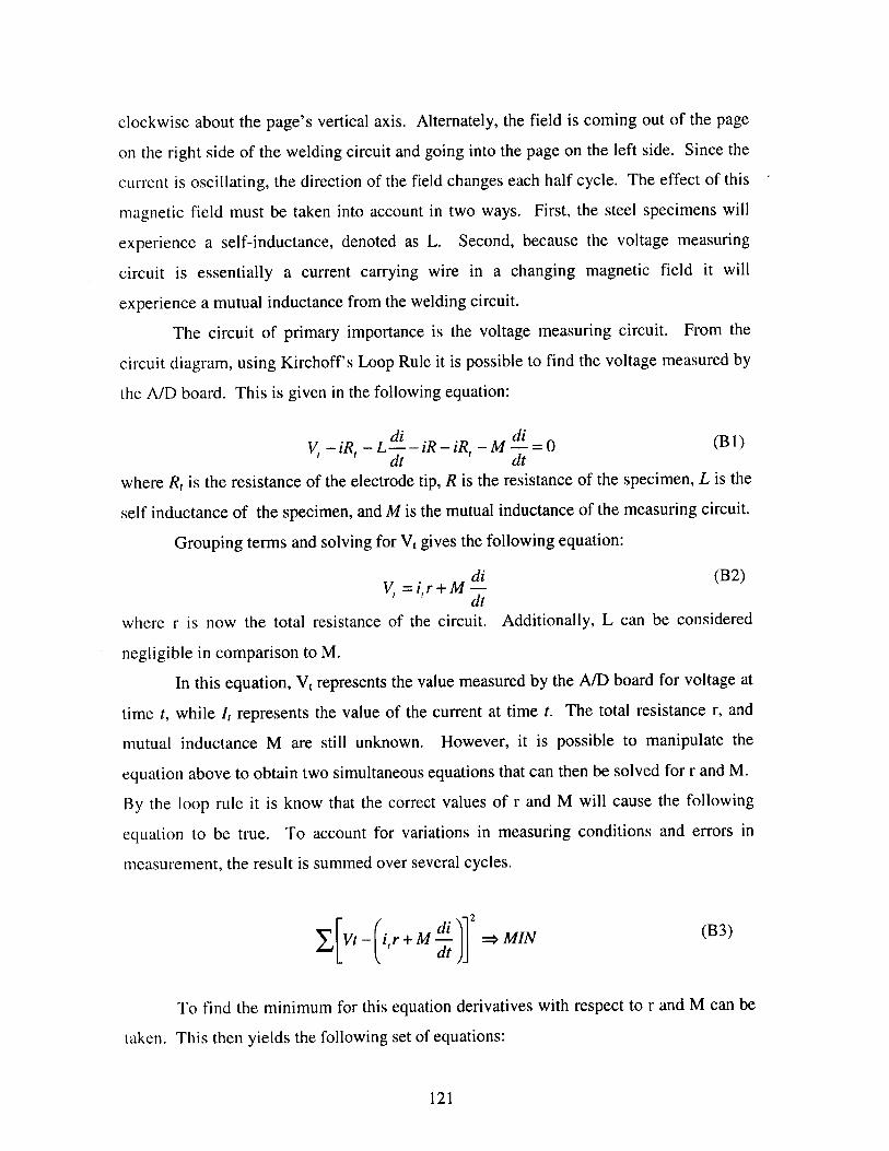
clockwise about the page's vertical axis. Alternately, the field is coming out of the page
on the right side of the welding circuit and going into the page on the left side. Since the
current is oscillating, the direction of the field changes each half cycle. The effect of this
magnetic field must be taken into account in two ways. First, the steel specimens will
experience a self-inductance, denoted as L. Second, because the voltage measuring
circuit is essentially a current carrying wire in a changing magnetic field it will
experience a mutual inductance from the welding circuit.
The circuit of primary importance is the voltage measuring circuit. From the
circuit diagram, using Kirchoff's Loop Rule it is possible to find the voltage measured by
the A/D board. This is given in the following equation:
V1 -iR -Ld-iR-iR -M-=0 (B1)dt dt
where R, is the resistance of the electrode tip, R is the resistance of the specimen, L is the
self inductance of the specimen, and M is the mutual inductance of the measuring circuit.
Grouping terms and solving for Vt gives the following equation:
di (B2)V, =i,r+M -
dtwhere r is now the total resistance of the circuit. Additionally, L can be considered
negligible in comparison to M.
In this equation, Vt represents the value measured by the A/D board for voltage at
time t, while I, represents the value of the current at time t. The total resistance r, and
mutual inductance M are still unknown. However, it is possible to manipulate the
equation above to obtain two simultaneous equations that can then be solved for r and M.
By the loop rule it is know that the correct values of r and M will cause the following
equation to be true. To account for variations in measuring conditions and errors in
measurement, the result is summed over several cycles.
Vt ir+M i =>MIN (B3)dt
To find the minimum for this equation derivatives with respect to r and M can be
taken. This then yields the following set of equations:
121

df _:2 F -(ir+M dhl[ v (. +d Mdi (4dr d dr dr di
df 2[ (rM di dV_ i,r + di (B5)dM dt dM dM dt
df _ di+ (di r+M d l=0 (B6)dM 'dt 'dt dt )
df= 1[-Vi, + i,2 r+iM di =0 (B7)dr dt)_
Before calculations can be made to determine values for r and M using these
equations, the value of Vt and I, must be converted into volts and amps respectively.
Calculating the true voltage is relatively simple as the A/D board uses only a simple gain
factor when measuring voltage. The gain of the board is set via the monitoring program
to a value of 2. This means that the 12-bit A/D board will use a full range scale of ±2.5
volts. To calculate Vt, the measured value from the board, Vmeas, is multiplied by 2.5 V
and divided by 2048, the number of discrete steps for half of a 12-bit converter.
Vt=Viea 2.5 (B8)2048
The actual time of each sampling is obtained by dividing the sample number by
the sampling frequency, 2400 Hz:
t = samp# (B9)2400
Since the A/D board can only sample one value at a time, the sampling order for a
given time period is as follows: Cl -> V -> C2 . To estimate the current at the time V is
taken, the measured values are averaged to give:
- (c + c2 ) (B10)C =2
122
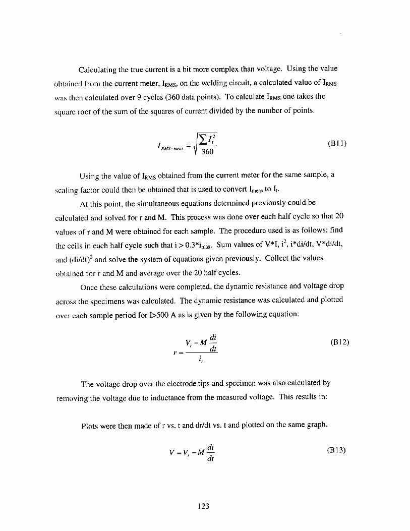
Calculating the true current is a bit more complex than voltage. Using the value
obtained from the current meter, IRMS, on the welding circuit, a calculated value of IRMS
was then calculated over 9 cycles (360 data points). To calculate IRMS one takes the
square root of the sum of the squares of current divided by the number of points.
IRMS-ea=I - (B 11)- 360
Using the value of IRMS obtained from the current meter for the same sample, a
scaling factor could then be obtained that is used to convert Imeas to It.
At this point, the simultaneous equations determined previously could be
calculated and solved for r and M. This process was done over each half cycle so that 20
values of r and M were obtained for each sample. The procedure used is as follows: find
the cells in each half cycle such that i > 0.3*imax. Sum values of V*I, i2, i*di/dt, V*di/dt,
and (di/dt) 2 and solve the system of equations given previously. Collect the values
obtained for r and M and average over the 20 half cycles.
Once these calculations were completed, the dynamic resistance and voltage drop
across the specimens was calculated. The dynamic resistance was calculated and plotted
over each sample period for 1>500 A as is given by the following equation:
diVt -M (B 12)
r =dti,
The voltage drop over the electrode tips and specimen was also calculated by
removing the voltage due to inductance from the measured voltage. This results in:
Plots were then made of r vs. t and dr/dt vs. t and plotted on the same graph.
V =V -M i (B13)dt
123

Current and voltage waveforms were also plotted against t on the same graph.
The voltage plotted in this case was that obtained in the equation above. This voltage
was also plotted vs. current. These plots can then be used to determine if the correct
value for M has been obtained. Two distinct features can be noted if the proper value of
M has been used. First, on the waveforms vs. time plot, the peaks of each waveform
should occur at the same time if the inductance effect has been successfully removed
from the measured voltage. Second, in the plot of V vs. I, hysteresis effects from the
inductance will show up. When the inductance is removed, the voltage will be seen to
vary linearly with the current.
124

Appendix CParameter Files for Simulator and Show Out Programs
The following files are required for the proper operation of the simulation
program. These files are explained in detail in Chapter 3 and are list here for reference.
C.1 BSOGBE.dat
"*** Control data
-10.41, 0.320.0050.01601.250.020000.00.6540.0
22.1280.00.30.0971602000002419.5906.00"Rtype200"10.254.520.0"1 SPCC "
for 0.97mm bare steel sheets ***"/* place keeping parameter
/* dc-de (cm)
/* Maximum current value (A)
/* Electrode tip resistance (UQ)
/* Workpiece thickness (cm)
/* Electrode tip configuration file
/* Initial workpiece temperature 0C
/* Material type
Bsogbe.dat is the control file for the simulation program. The parameters that are
identified above are those that need to be configured correctly for proper operation of the
simulation program. From this investigation, the most important values were d, and de
which, combined as Ac had the greatest effect on the accuracy of the simulation results.
125
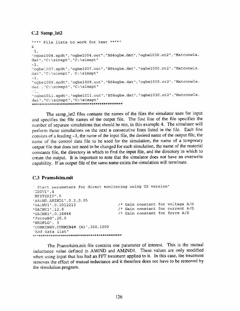
C.2 SampIst2
"*** File lists to work for test *
4-1,
"ogbel004.spdt" , "ogbelO04.out", "BS4ogbe.dat", "ogbel030.ot2", "Matconwla.
dat", "C:\simspt", "C:\simspt"-1,
"ogbelOO7.spdt", "ogbelO07.out", "BS4ogbe.dat", "ogbel030.ot2", "Matconwla.
dat", "C:\simspt", "C:\simspt"-1,
"ogbelOO8.spdt" , "ogbelO08.out", "BS4ogbe.dat", "ogbel030.ot2", "Matconwla.
dat","C:\simspt","C:\simspt"-1,
"ogbelOll.spdt" , "ogbelOll.out", "BS4ogbe.dat", "ogbel030.ot2", "Matconwla.
dat", "C:\simspt", "C:\simspt"** *** ******* ************** ******* *****
The sampjlst2 files contains the names of the files the simulator uses for inputand specifies the file names of the output file. The first line of the file specifies thenumber of separate simulations that should be run, in this example 4. The simulator willperform these simulations on the next n consecutive lines listed in the file. Each lineconsists of a leading -1, the name of the input file, the desired name of the output file, thename of the control data file to be used for the simulation, the name of a temporaryoutput file that does not need to be changed for each simulation, the name of the materialconstants file, the directory in which to find the input file, and the directory in which tocreate the output. It is important to note that the simulator does not have an overwritecapability. If an output file of the same name exists the simulation will terminate.
C.3 Prams4sim.mit
" Start parameters for direct monitoring using US version"
"IDIV1",4"NFSTSKIP" ,6'AMIND,AMIND1",0.2,0.05"GAINV1",0.0012213 /* Gain constant for voltage A/D
"GAINCl" ,12.O /* Gain constant for current A/D
"GAINX1",0.26866 /* Gain constant for force A/D
"ForceBS",20.0"NRDFLG", 3"CURMIN4V,CURMIN4R (A) ",300,1000
"End data list"
The Prams4sim.mit file contains one parameter of interest. This is the mutualinductance value defined in AMIND and AMINDL. These values are only modifiedwhen using input that has had an FFT treatment applied to it. In this case, the treatmentremoves the effect of mutual inductance and it therefore does not have to be removed bythe simulation program.
126

C.4 matconwla.dat
"MATCONSET.DAT for Zinc coated steel sheets"
"<Resistivity ; micro-Ohm*cm T,A,B,C; A*T*T+B*T+C>"
-200.0, 10.56E-5, 3.575E-2,800.0, 0.0 2.875E-2,
1200.0, 0.0, 0.0,
1530.0, 0.0, 2.0,
1590.0, 0.0, 0.0,
3000.0, 0.0, 0.0,
"<Thermal conductivity; J/cm/
-200.0, -3.48E-7, -1.04E-4,
400.0, -3.13E-7, -4.18E-5,
800.0, 0.0, 0.0,
1530.0, 0.0, 1.56E-2,
1600.0, 0.0, 0.0,
3000.0, 0.0, 0.0,
"<Specific heat; J/g/K>
-200.0, 1.28E-7, 3.2E-4,400.0, 7.73E-7, 0.0,
600.0, 0.0, 3.07E-3,
750.0, 0.0, -5.43E-3,
850.0, 0.0, 0.0,
1530.0, 0.0,"<Other setting cons
1,"RMTEMP",20.0
2, "MCOD",550.0
3, "TMELT",1530.0
4, "THAZ",723.0
5," HL",415.6258,"DENSITY",7.7
11,"ALPHA",14.5E-6
12," C1 ",4580.013," C2 ", 230.0
14," AM1", 6.2
15," QE ",309000.016,"GASR", 8.31417," A ", 5.0
18," AM2", 5.821," TS ", 550.0
22," YS ", 234.0
23,"ALPHSIG",0.010
24,"SIGMIN", 1.0
25, "TEMPl", 890.026, "TEMP2" , 1420.0
31, "TSOFT", 538.0
32,"RFHIGHT", 0.002
33,"CON4SFR",200.034," RO ", 0.035," POW ", 0.3
36," El ",2100000.037," E2 ",1200000.0
38,"THMIN", 0.38
39,"CON4ELS", 0.8141, "FSP1 ", 1.5
42,"FSP2 ", 0.08
.0,stants>"
15.090.4
124.0-2940.0
360.0360.0
s/K>"0.5220.4920.273
-23.5950.8910.891
0.4490.449
-1.095.290.6690.669
/* Ambient room temperature 0C
/* Melting temperature 0C
/* Boundary temperature of HAZ 0C
/* Tensile stress of material (MPa)
/* Yield stress of material (MPa)
/* Temperature at which metal softens
127

43, "FSP3 ", 2.644, "FSP4 ", 0.745, "FSP5 ", 0.046, "CUSH ", 0.827747,"CUHC ", 0.7548, "ALPH4CUK" ,0.15
49, "TRNST4CUK",1000.0
50, "COFF4NWCUK",0.859999, "End" 999
The matconwla.dat file specifies the various material constants used by thesimulation program. Three of these properties are considered to be temperaturedependent and are given different parameter values based on the mesh point temperature.Interpolation is used to obtain parameter values for temperatures not explicitly listed in
the table. The remaining parameters are independent of temperature. The moreimportant parameters are highlighted above.
128

C.5 Simulation results file
The lines below show a sample of the output generated by the simulationprogram. The data is generated for every 1/8 cycle from time zero to the end of the weld.
Examples are shown below at t = 0, t = I cycle, and t = 10 cycles. The values on the
output below, beginning with the line below 91 indicate the cycle time which the data
represents, the RMS current, IRMS, the contact diameter at the faying surface, de, thecontact diameter at the electrode, de, the nugget diameter, dn, the HAZ diameter, dHAZ, thepenetration depth of the nugget, pn, and the penetration depth of the HAZ, PHAZ. The
values following represent the temperatures at the mesh points within the workpiece.
Across the page represents the thickness of the workpiece and down the page representsthe radial direction of the weld. In the results from cycles I and 10 it can be seen that the
temperature is greatest near the center of the weld and decreases in the vertical and radial
direction. The results from later cycles also show how the nugget diameter, penetration
depth, and HAZ change with time.
<Window Ver 1.2> Electrode tip SHAPE; C:\simspt\Rtype200
Input data; C:\simspt\ogbel004.spdt
Material; SPCC
CALC. range;.78000 Radius of pre-weld;
.25000 Weld pitch; 4.50000
.02000 .00970 40 11
11 57 11 57 20 29
91
t IRMS dc de dn dAz Pn PHAz
.000 11.6 .00032 27.86 .3600 .3000 .0000 .0000 .0000 .0000
20.00 .32578 20.00 20.00 20.00 20.00 277.473 138.737
173.43520 1.0000220.00 20.00 20.00 20.00 20.00 20.00 20.00 20.00 20.00 20.00 20.00
20.00 20.00 20.00 20.00 20.00 20.00 20.00 20.00 20.00 20.00 20.00
20.00 20.00 20.00 20.00 20.00 20.00 20.00 20.00 20.00 20.00 20.00
20.00 20.00 20.00 20.00 20.00 20.00 20.00 20.00 20.00 20.00 20.00
20.00 20.00 20.00 20.00 20.00 20.00 20.00 20.00 20.00 20.00 20.00
20.00 20.00 20.00 20.00 20.00 20.00 20.00 20.00 20.00 20.00 20.00
20.00 20.00 20.00 20.00 20.00 20.00 20.00 20.00 20.00 20.00 20.00
20.00 20.00 20.00 20.00 20.00 20.00 20.00 20.00 20.00 20.00 20.00
20.00 20.00 20.00 20.00 20.00 20.00 20.00 20.00 20.00 20.00 20.00
20.00 20.00 20.00 20.00 20.00 20.00 20.00 20.00 20.00 20.00 20.00
20.00 20.00 20.00 20.00 20.00 20.00 20.00 20.00 20.00 20.00 20.00
20.00 20.00 20.00 20.00 20.00 20.00 20.00 20.00 20.00 20.00 20.00
20.00 20.00 20.00 20.00 20.00 20.00 20.00 20.00 20.00 20.00 20.00
20.00 20.00 20.00 20.00 20.00 20.00 20.00 20.00 20.00 20.00 20.00
20.00 20.00 20.00 20.00 20.00 20.00 20.00 20.00 20.00 20.00 20.00
20.00 20.00 20.00 20.00 20.00 20.00 20.00 20.00 20.00 20.00 20.00
20.00 20.00 20.00 20.00 20.00 20.00 20.00 20.00 20.00 20.00 20.00
20.00 20.00 20.00 20.00 20.00 20.00 20.00 20.00 20.00 20.00 20.00
20.00 20.00 20.00 20.00 20.00 20.00 20.00 20.00 20.00 20.00 20.00
20.00 20.00 20.00 20.00 20.00 20.00 20.00 20.00 20.00 20.00 20.00
20.00 20.00 20.00 20.00 20.00 20.00 20.00 20.00 20.00 20.00 20.00
20.00 20.00 20.00 20.00 20.00 20.00 20.00 20.00 20.00 20.00 20.00
20.00 20.00 20.00 20.00 20.00 20.00 20.00 20.00 20.00 20.00 20.00
20.00 20.00 20.00 20.00 20.00 20.00 20.00 20.00 20.00 20.00 20.00
129

20.0020.0020.0020.0020.0020.0020.0020.0020.0020.0020.0020.0020.0020.0020.0020.00
20.0020.0020.0020.0020.0020.0020.0020.0020.0020.0020.0020.0020.0020.0020.0020.00
20.0020.0020.0020.0020.0020.0020.0020.0020.0020.0020.0020.0020.0020.0020.0020.00
1.000 523.5.3464 .0000199.57 829.83833.02 842.13
901.03833.02 842.13
901.03828.88 836.90
944.49821.50 827.93
965.10818.49 819.45
1004.54818.77 813.55
1191.10811.12 800.21
1512.90836.28 812.74
1378.51740.93 738.27
961.44554.61 525.08
600.72489.15 419.03
270.49199.57 172.90
112.4470.92 67.57
53.0534.61 34.10
30.5124.20 24.10
23.2521.20 21.18
20.9820.34 20.34
20.2920.10 20.10
20.0920.03 20.03
20.0220.01 20.01
20.0120.00 20.00
20.00
20.0020.0020.0020.0020.0020.0020.0020.0020.0020.0020.0020.0020.0020.0020.0020.00
20.0020.0020.0020.0020.0020.0020.0020.0020.0020.0020.0020.0020.0020.0020.0020.00
2222222222222222
.05109 97.1940 833
1029.48 99866.25 918.75698.38 378.11866.25 918.75698.38 378.11865.01 913.29726.81 463.89847.49 883.88745.78 512.27826.08 846.90814.55 621.35805.81 810.611004.14 629.79778.88 770.391134.08 434.66755.78 706.141417.27 493.44662.55 580.941182.19 829.83462.01 406.02768.49 1029.48326.99 261.75315.72 345.73143.99 122.08120.88 125.0561.71 56.2153.7232.96 31.7130.6323.87 23.6023.2821.13 21.0720.9920.33 20.3120.2920.09 20.0920.0920.03 20.0320.0220.01 20.0120.0120.00 20.0020.00
0.00 20.00 20.00 20.00 20.00 20.00 20.00 20.00 20.00 20.00 20.00 20.00 20.00 20.00 20.00 20.00 2
.60
.02
.578974.31
0.000.000.000.000.000.000.000.000.000.000.000.000.000.000.000.00
20.0020.0020.0020.0020.0020.0020.0020.0020.0020.0020.0020.0020.0020.0020.0020.00
.4200378.11
49.7891022.00
20.0020.0020.0020.0020.0020.0020.0020.0020.0020.0020.0020.0020.0020.0020.0020.00
.3600.23955
176.
20.0020.0020.0020.0020.0020.0020.0020.0020.0020.0020.0020.0020.0020.0020.0020.00
20.0020.0020.0020.0020.0020.0020.0020.0020.0020.0020.0020.0020.0020.0020.0020.00
.0000489.15
65910 1.000051042.73 1012.36
974.31 1022.00 1042.73 1012.36
970.41 1026.14 1059.06 1041.99
941.99 1002.66 1051.44 1054.81
886.92 954.84 1025.64 1062.79
843.16 911.74 1028.09 1139.88
794.90 887.41 1080.99 1366.42
696.23 736.38 864.80 1091.92
545.12 554.00 616.67 752.92
372.41 369.16 401.70 476.74
224.08 209.06 213.13 234.27
108.03 101.10 100.34 104.64
52.19 49.93
30.70 30.07
23.36 23.20
21.02 20.98
20.30 20.29
20.09 20.08
20.03 20.02
20.01 20.01
20.00 20.00
49.32 50.03 51.53
29.84 29.94 30.22
23.13 23.14 23.19
20.96 20.96 20.97
20.29 20.29 20.29
20.08 20.08 20.08
20.02 20.02 20.02
20.01 20.01 20.01
20.00 20.00 20.00
130

20.00 20.0020.00
20.00 20.0020.00
20.00 20.0020.00
20.00 20.0020.00
20.00 20.0020.00
20.00 20.0020.00
20.00 20.0020.00
20.00 20.0020.00
20.00 20.00
20.0020.0020.0020.0020.0020.0020.0020.0020.0020.0020.0020.0020.0020.0020.0020.0020.00
20.00 20.0020.00 20.00 20.00
20.0020.00 20.00
20.0020.00 20.00
20.0020.00 20.00
20.0020.00 20.00
20.0020.00 20.00
20.0020.00 20.00
20.0020.00 20.00
20.0020.00 20.00
20.0020.00 20.00
20.00
10.000 .0.1261 .1940885.91 89.2461774.57 1768.86
1149.981774.57 1768.86
1149.981774.78 1769.11
1146.111775.20 1769.60
1139.031775.75 1770.30
1127.891776.07 1770.81
1111.991775.03 1769.93
1093.871771.31 1766.26
1082.961763.90 1758.90
1071.321752.14 1747.04
1057.42
20.00 20.00 20.00
20.00 20.00 20.00
20.00 20.00 20.00
20.00 20.00 20.00
20.00 20.00 20.00
20.00 20.00 20.00
20.00 20.00 20.00
20.00 20.00 20.00
20.00 20.00 20.00
20.00 20.00 20.0020.0020.00 20.00 20.00 20.0020.0020.0020.0020.0020.0020.0020.0020.0020.0020.0020.0020.0020.0020.0020.0020.0020.00
.000001774.57
44.6231751.54891.611751.54891.611751.89888.231752.53881.981753.66872.861754.73860.561754.46846.661750.90833.591743.73820.581731.58806.41
20.00 20.00 20.00
20.00 20.00 20.00
20.00 20.00 20.00
20.00 20.00 20.00
20.00 20.00 20.00
20.00 20.00 20.00
20.00 20.00 20.00
20.00 20.00 20.00
87.04637.73
.6750
20.00 20.00 20.00
20.00 20.00 20.00
20.00 20.00 20.00
20.00 20.00 20.00
20.00 20.00 20.00
20.00 20.00 20.00
20.00 20.00 20.00
20.00 20.00 20.00
20.00 20.00 20.00
20.00 20.00 20.00
20.00 20.00 20.00
20.00 20.00 20.00
20.00 20.00 20.00
20.00 20.00 20.00
20.00 20.00 20.00
20.00 20.00 20.00
20.00 20.00 20.00
20.00 20.00 20.00
20.00 20.00 20.00
6150 6200.41300 1414.02 1146.39
.7283435.17
180.95770 1.000101721.82637.731721.82637.731722.25635.271723.04630.761724.91624.371727.00616.021728.21606.201724.88595.151717.91582.601705.61568.27
1677.97 1617.94
1677.97 1617.94
1678.37 1617.72
1679.30 1618.30
1561.35 1401.68
1561.35 1401.68
1559.96 1397.91
1557.03 1390.93
1682.02 1618.90 1552.69 1378.50
1685.65 1624.26 1544.27 1357.30
1690.83 1641.45 1530.00 1321.14
1688.47 1642.84 1529.94 1312.45
1681.52 1637.07 1529.76 1305.70
1668.99 1620.76 1500.48 1289.80
131

1736.41 1731.03 1714.97 1688.13 1648.67 1605.01 1482.90 1273.191041.20 791.39 553.92
1717.35 1711.85 1695.07 1666.13 1622.56 1589.30 1470.38 1258.661037.74 776.98 533.71
1694.35 1689.11 1673.30 1648.22 1603.29 1568.78 1444.38 1236.481018.77 759.46 514.12
1665.12 1661.32 1649.67 1626.06 1594.99 1529.79 1381.10 1208.841003.77 746.75 497.31
1623.35 1623.29 1609.82 1585.05 1530.29 1443.23 1333.96 1190.691008.37 753.63 471.70
1556.81 1560.79 1529.88 1485.42 1421.72 1347.08 1261.36 1160.831017.95 757.30 435.17
1414.02 1381.13 1332.73 1274.16 1212.52 1152.32 1095.92 1043.22991.58 917.95 885.91
1146.39 1113.64 1050.52 992.75 942.94 900.42 864.98 835.74815.71 804.37 800.91
771.24 759.73 737.42 713.11 690.11 669.61 652.00 638.61628.07 620.00 617.82
539.63 537.57 532.24 525.00 517.05 509.23 502.16 496.31491.94 489.21 488.31
412.06 411.35 409.38 406.52 403.19 399.76 396.56 393.84391.79 390.52 390.09
323.64 323.35 322.53 321.30 319.81 318.24 316.74 315.45314.45 313.83 313.61
257.90 257.77 257.40 256.84 256.16 255.42 254.71 254.08253.59 253.28 253.18
207.29 207.24 207.07 206.81 206.48 206.13 205.78 205.48205.24 205.09 205.03
167.64 167.61 167.53 167.41 167.25 167.08 166.91 166.76166.65 166.57 166.54
136.28 136.26 136.22 136.16 136.09 136.01 135.92 135.85135.79 135.76 135.74
111.37 111.37 111.35 111.32 111.28 111.24 111.20 111.17111.14 111.12 111.11
91.59 91.58 91.57 91.56 91.54 91.52 91.50 91.48 91.4791.46 91.46
75.88 75.88 75.88 75.87 75.86 75.85 75.84 75.83 75.8375.82 75.82
63.46 63.46 63.45 63.45 63.45 63.44 63.44 63.43 63.4363.43 63.43
53.67 53.67 53.66 53.66 53.66 53.66 53.66 53.65 53.6553.65 53.65
46.00 46.00 45.99 45.99 45.99 45.99 45.99 45.99 45.9945.99 45.99
40.03 40.03 40.03 40.03 40.03 40.03 40.03 40.03 40.0340.03 40.02
35.43 35.43 35.43 35.43 35.43 35.43 35.43 35.43 35.4335.43 35.43
31.95 31.95 31.95 31.95 31.95 31.95 31.95 31.95 31.9531.95 31.95
29.36 29.36 29.36 29.36 29.36 29.36 29.36 29.36 29.3629.36 29.36
27.50 27.50 27.50 27.50 27.50 27.50 27.50 27.50 27.5027.50 27.50
26.26 26.26 26.26 26.26 26.26 26.26 26.26 26.26 26.2626.26 26.26
25.56 25.56 25.56 25.56 25.56 25.56 25.56 25.56 25.5625.56 25.56
25.33 25.33 25.33 25.33 25.33 25.33 25.33 25.33 25.3325.33 25.33
132

C.6 ParamSet4ADC_1.dat
"Test Parameter data"
10,6030000,2400,600.0012213,11.99,0.268666, 6203050.0,500.0
/* Weld time(cycles), Line Frequency/* Sampling Rate, Scanning Rate/* Gain of Voltage, Current, and Force
/* FFT cutoff frequency
The above file is used in the FFT treatment of the welding monitoring data. Thevalues in the file are used to convert the monitoring data to values of current, voltage, andforce in SI units. The FFT treatment is then applied based on the cutoff frequency. Thesampling rate is the frequency of A/D conversions performed during data capturing inhertz and the scanning rate is the frequency with which the entire bank of A/D inputs issampled, also in hertz.
133