Portland State University Portland State University

PDXScholar PDXScholar

Community Health Faculty Publications and Presentations School of Community Health

1-2015

An Introduction to the Loop Analysis of Qualitatively An Introduction to the Loop Analysis of Qualitatively

Specified Complex Causal Systems Specified Complex Causal Systems

Alexis Dinno Portland State University

Follow this and additional works at: https://pdxscholar.library.pdx.edu/commhealth_fac

Part of the Community Psychology Commons

Let us know how access to this document benefits you.

Citation Details Citation Details Dinno, A. (2015) An Introduction to the Loop Analysis of Qualitatively Specified Complex Causal Systems. Invited Presentation. Systems Science Graduate Program Seminar. Portland, OR.

This Presentation is brought to you for free and open access. It has been accepted for inclusion in Community Health Faculty Publications and Presentations by an authorized administrator of PDXScholar. Please contact us if we can make this document more accessible: pdxscholar@pdx.edu.

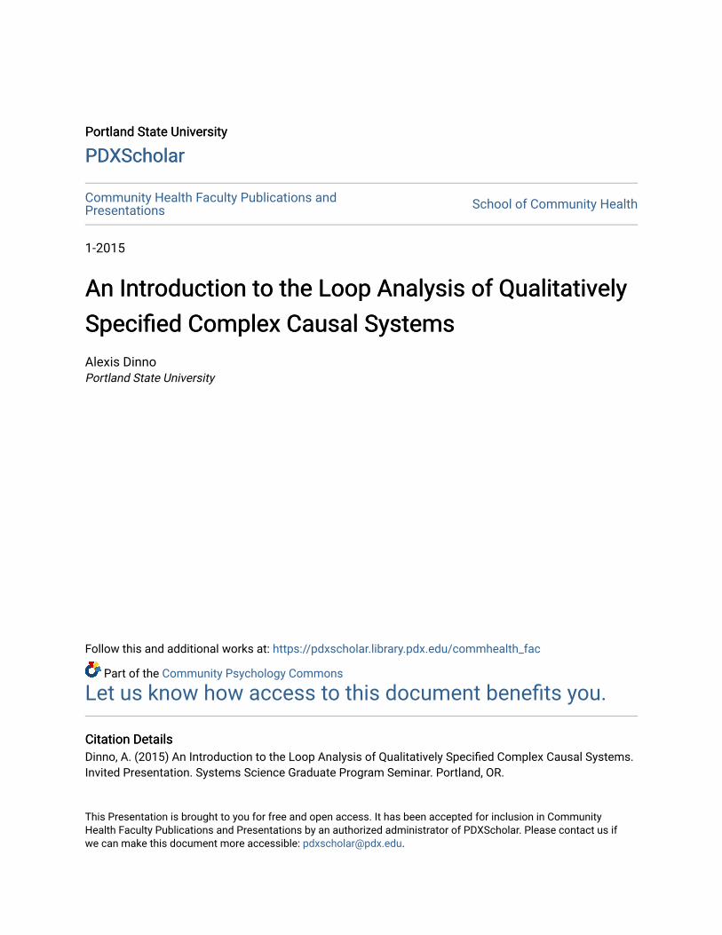
AN INTRODUCTION TO THE LOOP ANALYSIS OF QUALITATIVELY

SPECIFIED COMPLEX CAUSAL SYSTEMS “Things are like other things; this makes science possible. Things are unlike other things; this makes science neccesary.” —RICHARD LEVINS ALEXIS DINNO, C.AZ.AM., SC.D., M.P.H., M.E.M., I.O.U., ETC JANUARY 9, 2015

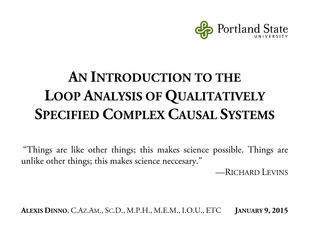
ORIGINS OF LOOP ANALYSIS 2 Developed by population biologist Richard Levins in the late 1960s Population dynamics of organisms in changing environments Deviates from Sewall Wright’s causal path analysis from the 1920’s Influenced by S. J. Mason’s theoretical work on signal flow graphs from the 1950’s Published mostly in population biology/population ecology, but also:

• Physical geography/hydrogeology • Chemical engineering (bioreactor stability) • Nuclear engineering (fault identification) • Social ecology/social epidemiology and infectious disease epidemiology

“How much can we get away with not knowing, yet still produce insights about nature?”

MOTIVATIONS: FIRST PART 3 MY INTEREST Human experience causes behavior change Human behavior causes environmental change Environmental change causes human experience How to analyze? PROBLEMS WITH TRADITIONAL CAUSAL STATISTICAL INFERENCE Does not describe system behavior, but rather terminal causal narratives Tries to “control for” endogeneity, to eliminate it from analysis “Bayesian network” and similar approaches choke on reciprocal causation Statistical models can be precise and realistic, but do not have generality LOOP ANALYSIS Describes several kinds of system behavior Makes endogeneity the object of substantive interest Reciprocal causation motivates the use of the method Loop models can be realistic and can have generality, but sacrifice quantitative precision

MOTIVATIONS: SECOND PART 4 “I SUPPOSE IT IS TEMPTING, IF THE ONLY TOOL YOU HAVE IS A HAMMER, TO TREAT EVERYTHING AS IF IT WERE A NAIL.” —ABRAHAM MASLOW Like theories, formal analytic models embed ontological and ideological assumptions. Loop analysis… …Rejects: The best path to knowledge of something is by breaking it apart into more fundamental pieces. (one type of reductionist ideology) …Embraces: The truth is the whole; all knowledge is radically incomplete. A path to knowledge of something may require examination of the relationships that define it. Reductionist methods may also contribute to knowledge. (holist ideology) …Permits: Inquiry can look at system phenomena from both the inside and the outside (disciplinary boundaries, model assumptions).

MOTIVATIONS: THIRD PART 5 HYPOTHESES MOTIVATED BY LOOP ANALYSIS

What is the predicted change in one variable in the system, given an input at any point or combination of points in the system?

What is the predicted bivariate correlation between two variables in the system given perturbation?

Do system inputs spread out across all variables, or sink into a few?

Are some variables susceptible or resistant to change?

Is the system stable? (does it tend to remain “near” its equilibrium point in the sense of Lyapunov stability)

Does system behavior depend upon particular relationships?

How does system behavior change when the variables or relationships comprising it change?

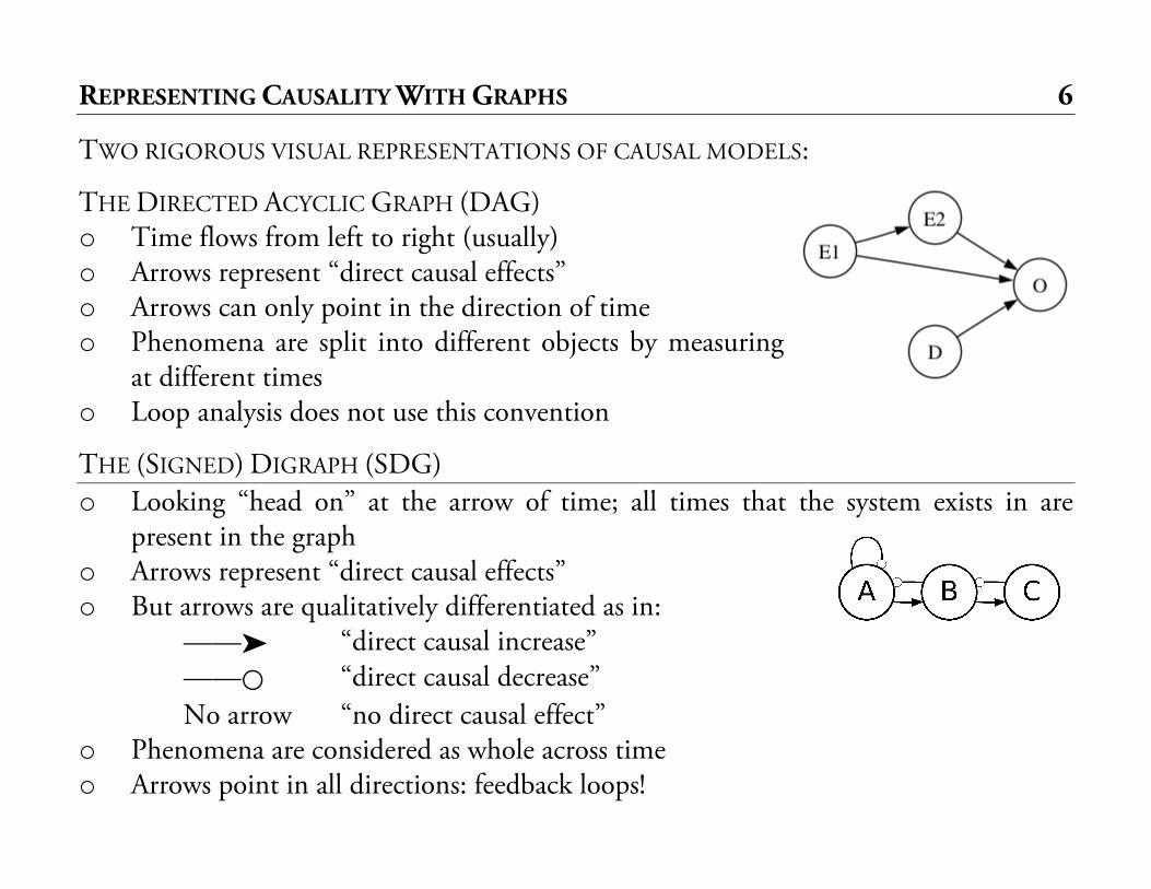
REPRESENTING CAUSALITY WITH GRAPHS 6

TWO RIGOROUS VISUAL REPRESENTATIONS OF CAUSAL MODELS:

THE DIRECTED ACYCLIC GRAPH (DAG) o Time flows from left to right (usually) o Arrows represent “direct causal effects” o Arrows can only point in the direction of time o Phenomena are split into different objects by measuring

at different times o Loop analysis does not use this convention

THE (SIGNED) DIGRAPH (SDG) o Looking “head on” at the arrow of time; all times that the system exists in are

present in the graph o Arrows represent “direct causal effects” o But arrows are qualitatively differentiated as in: ——➤ “direct causal increase” —— “direct causal decrease”

No arrow “no direct causal effect” o Phenomena are considered as whole across time o Arrows point in all directions: feedback loops!

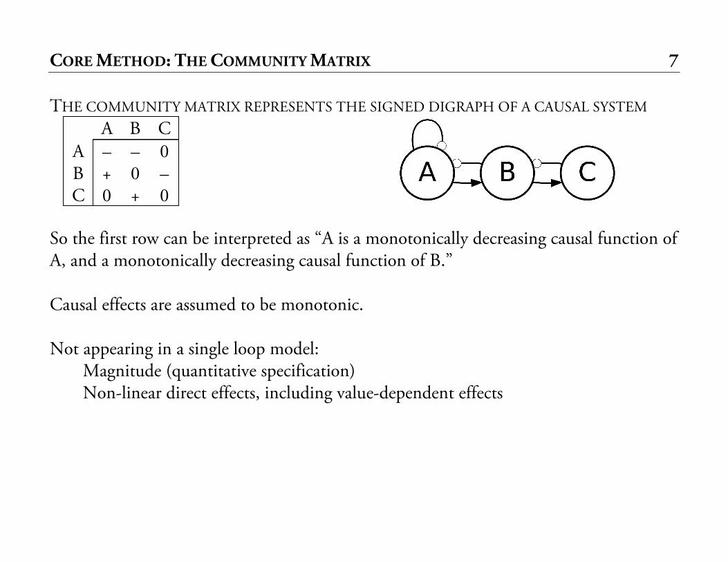
CORE METHOD: THE COMMUNITY MATRIX 7 THE COMMUNITY MATRIX REPRESENTS THE SIGNED DIGRAPH OF A CAUSAL SYSTEM

So the first row can be interpreted as “A is a monotonically decreasing causal function of A, and a monotonically decreasing causal function of B.” Causal effects are assumed to be monotonic. Not appearing in a single loop model: Magnitude (quantitative specification) Non-linear direct effects, including value-dependent effects

A B C A – – 0 B + 0 – C 0 + 0

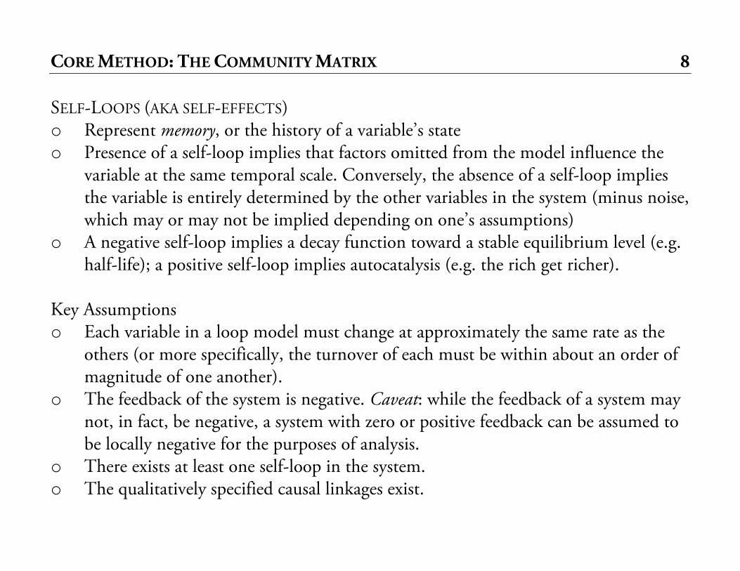
CORE METHOD: THE COMMUNITY MATRIX 8 SELF-LOOPS (AKA SELF-EFFECTS) o Represent memory, or the history of a variable’s state o Presence of a self-loop implies that factors omitted from the model influence the

variable at the same temporal scale. Conversely, the absence of a self-loop implies the variable is entirely determined by the other variables in the system (minus noise, which may or may not be implied depending on one’s assumptions)

o A negative self-loop implies a decay function toward a stable equilibrium level (e.g. half-life); a positive self-loop implies autocatalysis (e.g. the rich get richer).

Key Assumptions o Each variable in a loop model must change at approximately the same rate as the

others (or more specifically, the turnover of each must be within about an order of magnitude of one another).

o The feedback of the system is negative. Caveat: while the feedback of a system may not, in fact, be negative, a system with zero or positive feedback can be assumed to be locally negative for the purposes of analysis.

o There exists at least one self-loop in the system. o The qualitatively specified causal linkages exist.

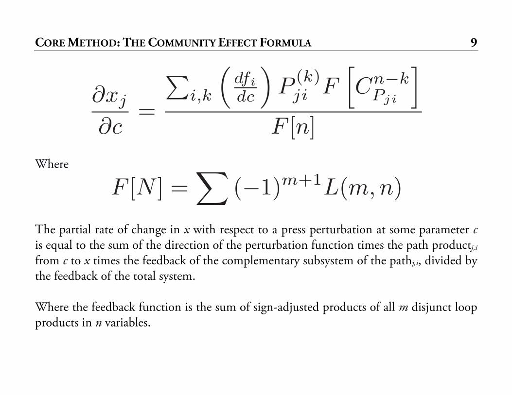
CORE METHOD: THE COMMUNITY EFFECT FORMULA 9

Where

The partial rate of change in x with respect to a press perturbation at some parameter c is equal to the sum of the direction of the perturbation function times the path productj,i from c to x times the feedback of the complementary subsystem of the pathj,i, divided by the feedback of the total system. Where the feedback function is the sum of sign-adjusted products of all m disjunct loop products in n variables.

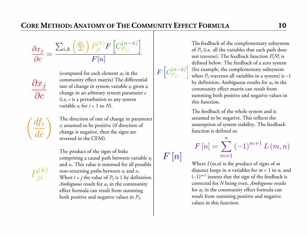
CORE METHOD: ANATOMY OF THE COMMUNITY EFFECT FORMULA 10

(computed for each element aij in the community effect matrix) The differential rate of change in system variable xj given a change in an arbitrary system parameter c (i.e. c is a perturbation to any system variable xi for i = 1 to N).

The direction of rate of change in parameter c; assumed to be positive (if direction of change is negative, then the signs are reversed in the CEM).

The product of the signs of links comprising a causal path between variable xj and xi. This value is summed for all possible non-returning paths between xj and xi. When i = j the value of Pij is 1 by definition. Ambiguous results for aij in the community effect formula can result from summing both positive and negative values in Pij.

The feedback of the complementary subsystem of Pij (i.e. all the variables that each path does not traverse). The feedback function F[N] is defined below. The feedback of a zero system (for example, the complementary subsystem when Pij traverses all variables in a system) is –1 by definition. Ambiguous results for aij in the community effect matrix can result from summing both positive and negative values in this function.

The feedback of the whole system and is assumed to be negative. This reflects the assumption of system stability. The feedback function is defined as:

Where L(m,n) is the product of signs of m disjunct loops in n variables for m = 1 to n, and (–1)m+1 insures that the sign of the feedback is corrected for N being even. Ambiguous results for aij in the community effect formula can result from summing positive and negative values in this function.

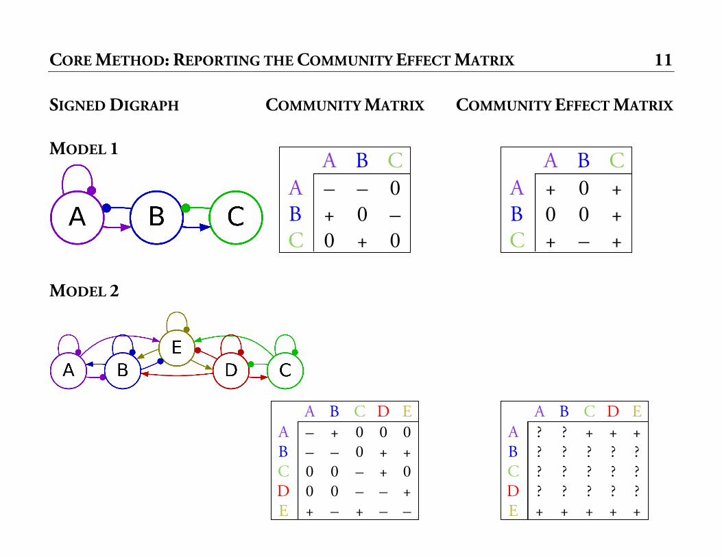
CORE METHOD: REPORTING THE COMMUNITY EFFECT MATRIX 11 SIGNED DIGRAPH COMMUNITY MATRIX COMMUNITY EFFECT MATRIX MODEL 1

MODEL 2

  A B C A – – 0 B + 0 – C 0 + 0

  A B C D E A ? ? + + + B ? ? ? ? ? C ? ? ? ? ? D ? ? ? ? ? E + + + + +

  A B C A + 0 + B 0 0 + C + – +

  A B C D E A – + 0 0 0 B – – 0 + + C 0 0 – + 0 D 0 0 – – + E + – + – –

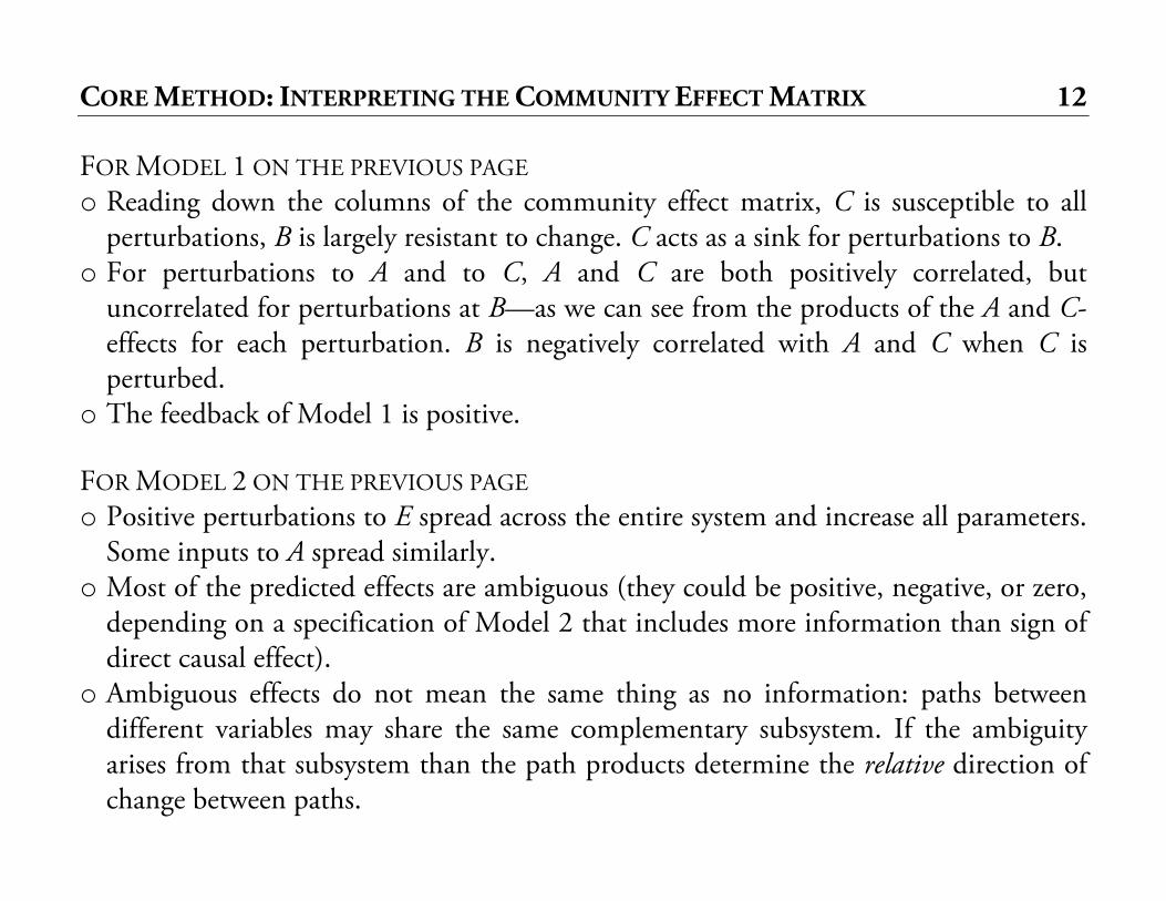
CORE METHOD: INTERPRETING THE COMMUNITY EFFECT MATRIX 12 FOR MODEL 1 ON THE PREVIOUS PAGE o Reading down the columns of the community effect matrix, C is susceptible to all

perturbations, B is largely resistant to change. C acts as a sink for perturbations to B. o For perturbations to A and to C, A and C are both positively correlated, but

uncorrelated for perturbations at B—as we can see from the products of the A and C-effects for each perturbation. B is negatively correlated with A and C when C is perturbed.

o The feedback of Model 1 is positive. FOR MODEL 2 ON THE PREVIOUS PAGE o Positive perturbations to E spread across the entire system and increase all parameters.

Some inputs to A spread similarly. o Most of the predicted effects are ambiguous (they could be positive, negative, or zero,

depending on a specification of Model 2 that includes more information than sign of direct causal effect).

o Ambiguous effects do not mean the same thing as no information: paths between different variables may share the same complementary subsystem. If the ambiguity arises from that subsystem than the path products determine the relative direction of change between paths.

CORE METHOD: COMPUTATION OF THE COMMUNITY EFFECT MATRIX 13 For small systems (n < 6) computing by hand is relatively easy, but it can be error prone. For a fully-specified community matrix, computation time increases with size on the order of n2(f(n!)) and the computational complexity class of the function is #P. Computation time can be decreased by taking advantage of matrix connectance, ambiguity, and structure respectively: o Pruning of the search space for sets of disjoint loops spanning n parameters o Halting of calculations when ambiguous results first arise o Caching computation results on revisited paths and subsystems; this can be

extended to families of models sharing common variables Perhaps computable systems are unlikely to get much larger than a few dozen variables.

BROAD METHOD: GROUPING MODELS INTO ENSEMBLES 14 BY BUILDING MODEL ENSEMBLES, LOOP ANALYSIS ACCOMMODATES: o Competing hypotheses (e.g. disagreement or uncertainty about the sign or existence

of particular causal links) o Complex relationships (e.g. causal links that change, for example: value dependent

relationships) o Alternative network composition (e.g. introduction, merging, splitting or elimination

of variables. Thus, parallel networks may be modeled for heterogeneous actors.). INTERPRETING MODEL GROUPS: o Indicates the robustness or sensitivity of findings to changes in assumed model

structures. o Can be used to identify links or variables for which system behavior changes

dramatically, and indicates either highly varying nature, and/or critical priorities for further research.

o Models are not rejected in favor of a “winning” community matrix.

BROAD METHOD: MODEL ENSEMBLE EXAMPLE 15 Run competing views of a system comprising: • Individual residential depressive experiences • Neighborhood exit rate • Neighborhood death rate • Neighborhood vacancies • Individual social isolation • Neighborhood greenspace programs

See Loop Analyst

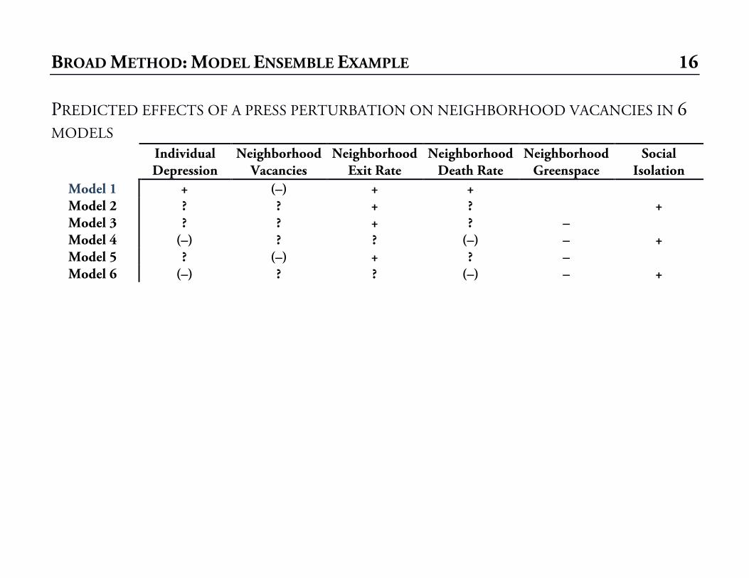
BROAD METHOD: MODEL ENSEMBLE EXAMPLE 16 PREDICTED EFFECTS OF A PRESS PERTURBATION ON NEIGHBORHOOD VACANCIES IN 6 MODELS

Individual Depression

Neighborhood Vacancies

Neighborhood Exit Rate

Neighborhood Death Rate

Neighborhood Greenspace

Social Isolation

Model 1 + (–) + + Model 2 ? ? + ? + Model 3 ? ? + ? – Model 4 (–) ? ? (–) – + Model 5 ? (–) + ? – Model 6 (–) ? ? (–) – +

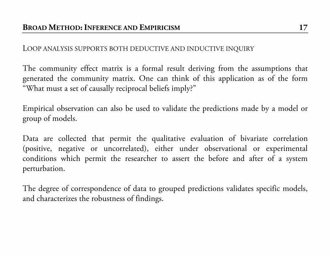
BROAD METHOD: INFERENCE AND EMPIRICISM 17 LOOP ANALYSIS SUPPORTS BOTH DEDUCTIVE AND INDUCTIVE INQUIRY The community effect matrix is a formal result deriving from the assumptions that generated the community matrix. One can think of this application as of the form “What must a set of causally reciprocal beliefs imply?” Empirical observation can also be used to validate the predictions made by a model or group of models. Data are collected that permit the qualitative evaluation of bivariate correlation (positive, negative or uncorrelated), either under observational or experimental conditions which permit the researcher to assert the before and after of a system perturbation. The degree of correspondence of data to grouped predictions validates specific models, and characterizes the robustness of findings.

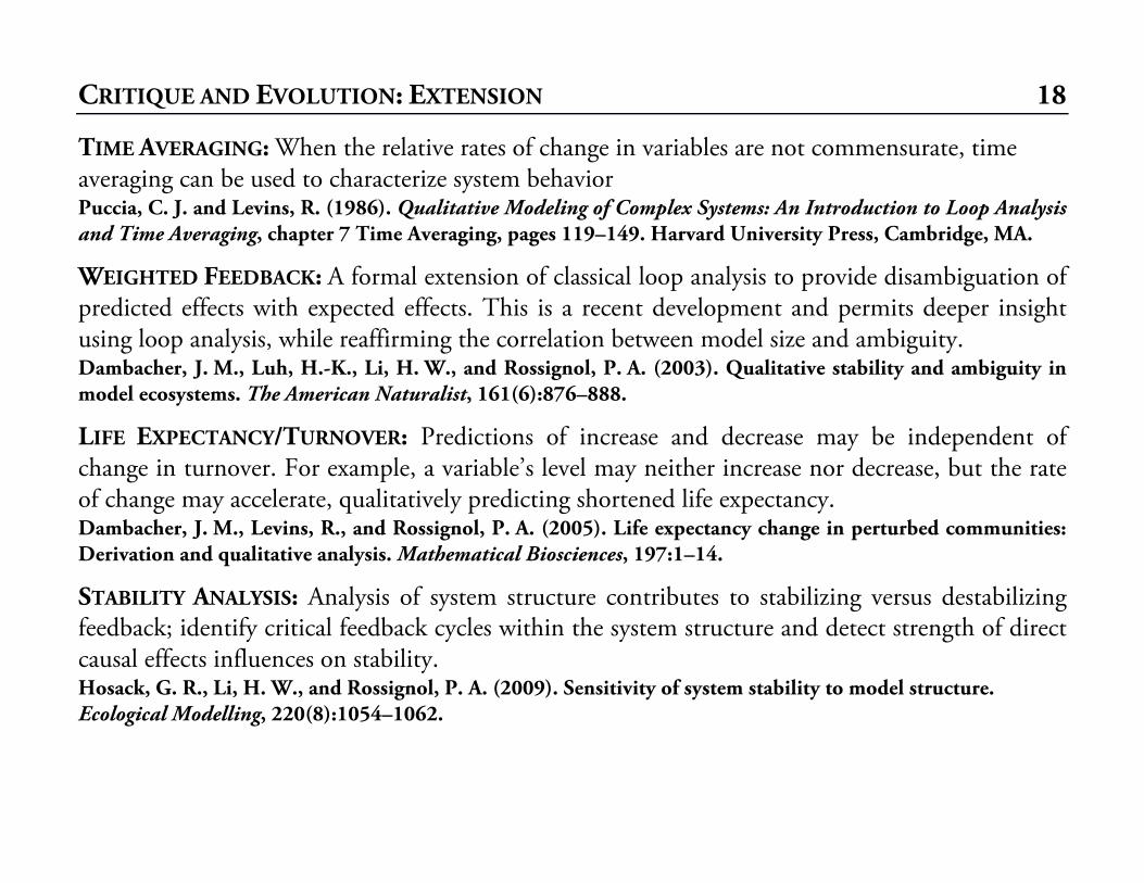
CRITIQUE AND EVOLUTION: EXTENSION 18

TIME AVERAGING: When the relative rates of change in variables are not commensurate, time averaging can be used to characterize system behavior Puccia, C. J. and Levins, R. (1986). Qualitative Modeling of Complex Systems: An Introduction to Loop Analysis and Time Averaging, chapter 7 Time Averaging, pages 119–149. Harvard University Press, Cambridge, MA.

WEIGHTED FEEDBACK: A formal extension of classical loop analysis to provide disambiguation of predicted effects with expected effects. This is a recent development and permits deeper insight using loop analysis, while reaffirming the correlation between model size and ambiguity. Dambacher, J. M., Luh, H.-K., Li, H. W., and Rossignol, P. A. (2003). Qualitative stability and ambiguity in model ecosystems. The American Naturalist, 161(6):876–888.

LIFE EXPECTANCY/TURNOVER: Predictions of increase and decrease may be independent of change in turnover. For example, a variable’s level may neither increase nor decrease, but the rate of change may accelerate, qualitatively predicting shortened life expectancy. Dambacher, J. M., Levins, R., and Rossignol, P. A. (2005). Life expectancy change in perturbed communities: Derivation and qualitative analysis. Mathematical Biosciences, 197:1–14.

STABILITY ANALYSIS: Analysis of system structure contributes to stabilizing versus destabilizing feedback; identify critical feedback cycles within the system structure and detect strength of direct causal effects influences on stability. Hosack, G. R., Li, H. W., and Rossignol, P. A. (2009). Sensitivity of system stability to model structure. Ecological Modelling, 220(8):1054–1062.

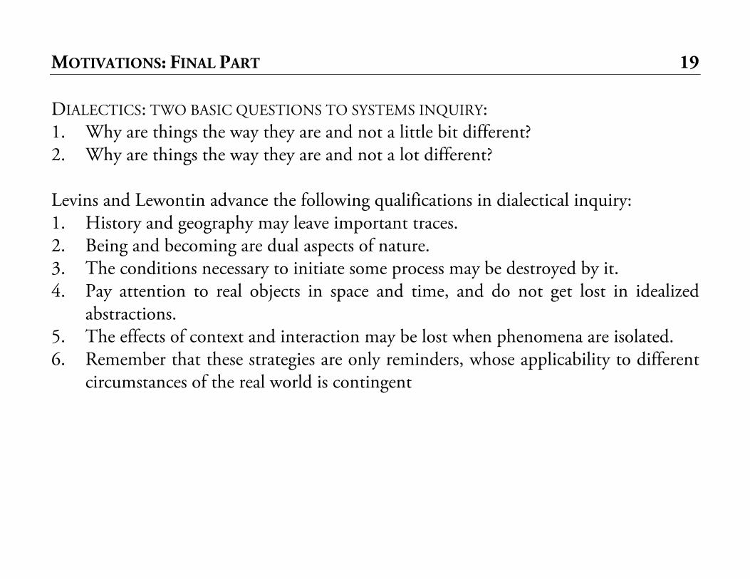
MOTIVATIONS: FINAL PART 19 DIALECTICS: TWO BASIC QUESTIONS TO SYSTEMS INQUIRY: 1. Why are things the way they are and not a little bit different? 2. Why are things the way they are and not a lot different? Levins and Lewontin advance the following qualifications in dialectical inquiry: 1. History and geography may leave important traces. 2. Being and becoming are dual aspects of nature. 3. The conditions necessary to initiate some process may be destroyed by it. 4. Pay attention to real objects in space and time, and do not get lost in idealized

abstractions. 5. The effects of context and interaction may be lost when phenomena are isolated. 6. Remember that these strategies are only reminders, whose applicability to different

circumstances of the real world is contingent

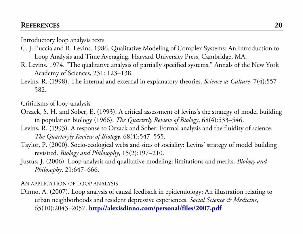
REFERENCES 20 Introductory loop analysis texts C. J. Puccia and R. Levins. 1986. Qualitative Modeling of Complex Systems: An Introduction to

Loop Analysis and Time Averaging. Harvard University Press, Cambridge, MA. R. Levins. 1974. "The qualitative analysis of partially specified systems." Annals of the New York

Academy of Sciences, 231: 123–138. Levins, R. (1998). The internal and external in explanatory theories. Science as Culture, 7(4):557–

582. Criticisms of loop analysis Orzack, S. H. and Sober, E. (1993). A critical assessment of levins’s the strategy of model building

in population biology (1966). The Quarterly Review of Biology, 68(4):533–546. Levins, R. (1993). A response to Orzack and Sober: Formal analysis and the fluidity of science.

The Quarteryly Review of Biology, 68(4):547–555. Taylor, P. (2000). Socio-ecological webs and sites of sociality: Levins’ strategy of model building

revisited. Biology and Philosophy, 15(2):197–210. Justus, J. (2006). Loop analysis and qualitative modeling: limitations and merits. Biology and

Philosophy, 21:647–666.

AN APPLICATION OF LOOP ANALYSIS Dinno, A. (2007). Loop analysis of causal feedback in epidemiology: An illustration relating to

urban neighborhoods and resident depressive experiences. Social Science & Medicine, 65(10):2043–2057. http://alexisdinno.com/personal/files/2007.pdf

SOFTWARE 21 SOFTWARE Dinno, Alexis. (2006). Loop Analyst. Version 1.2-3. Package for R: http://cran.r-project.org/web/packages/LoopAnalyst/index.html Dinno, Alexis. (2009). Stand alone GUI package for OS X Published: http://alexisdinno.com/LoopAnalyst Loop Group (Oregon State University). Web-based interface to Matlab loop analysis tools http://ipmnet.org/loop/

MY QUESTIONS FOR YOU 22 Could you see a role for loop analysis in the work that you do? Would an Introduction to Loop Analysis course detailing this method and elaborations on it appeal to you or your students?