An Introduction to Stochastic Control, withApplications to Mathematical Finance

Bernt ØksendalDepartment of Mathematics, University of Oslo, Norway

andNorwegian School of Economics (NHH),Bergen, Norway

Stochastic Processes and Applications,Ulan Bator, Mongolia, 29-31 July 2015

These lectures are partially based on joint works withAgnes Sulem, INRIA, Paris, France

On the wall of the entrance hall of the main building of theHumboldt University, Berlin (freely translated):

”For centuries scientists and philosophers have tried to understandthe world. Now is the time to control it!”

Karl Marx

Abstract

We give a short introduction to the stochastic calculus forIto-Levy processes and review briefly the two main methods ofoptimal control of systems described by such processes:

(i) Dynamic programming and the Hamilton-Jacobi-Bellman(HJB) equation

(ii) The stochastic maximum principle and its associatedbackward stochastic differential equation (BSDE).

The two methods are illustrated by application to the classicalportfolio optimization problem in finance. A second applicationis the problem of risk minimization in a financial market. Usinga dual representation of risk, we arrive at a stochasticdifferential game, which is solved by using theHamilton-Jacobi-Bellman-Isaacs (HJBI) equation, which is anextension of the HJB equation to stochastic differential games.

Introduction

The purpose of the course is to give a quick introduction tostochastic control of jump diffusions, with applications tomathematical finance, with emphasis on portfolio optimization andrisk minimization. The content of these lectures is the following:

In Section 2 we review some basic concepts and results from thestochastic calculus of Ito-Levy processes.

In Section 3 we present a portfolio optimization problem in anIto-Levy type financial market. We recognize this as a special caseof a stochastic control problem and we present the first generalmethod for solving such problems: Dynamic programming and theHJB equation. We show that if the system is Markovian, we canuse this method to solve the problem.

In Section 4 we study a risk minimization problem in the samemarket. By a general representation of convex risk measures, thisproblem may be regarded as a stochastic differential game, whichalso can be solved by dynamic programming (HJBI equation) if thesystem is Markovian.

Finally, in Section 5 we study the portfolio optimization problem bymeans of the second main stochastic control method: Themaximum principle. The advantage with this method is that it alsoapplies to non-Markovian systems.

Stochastic calculus for Ito-Levy processes

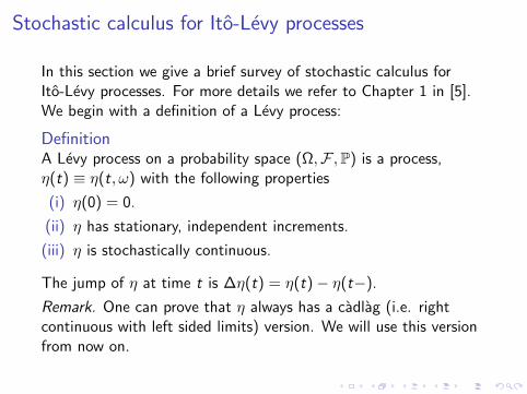
In this section we give a brief survey of stochastic calculus forIto-Levy processes. For more details we refer to Chapter 1 in [5].We begin with a definition of a Levy process:

DefinitionA Levy process on a probability space (Ω,F ,P) is a process,η(t) ≡ η(t, ω) with the following properties

(i) η(0) = 0.

(ii) η has stationary, independent increments.

(iii) η is stochastically continuous.

The jump of η at time t is ∆η(t) = η(t)− η(t−).

Remark. One can prove that η always has a cadlag (i.e. rightcontinuous with left sided limits) version. We will use this versionfrom now on.

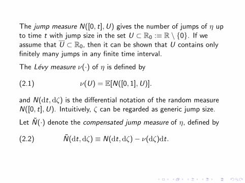
The jump measure N([0, t],U) gives the number of jumps of η upto time t with jump size in the set U ⊂ R0 :≡ R \ 0. If weassume that U ⊂ R0, then it can be shown that U contains onlyfinitely many jumps in any finite time interval.

The Levy measure ν(·) of η is defined by

ν(U) = E[N([0, 1],U)].(2.1)

and N(dt,dζ) is the differential notation of the random measureN([0, t],U). Intuitively, ζ can be regarded as generic jump size.

Let N(·) denote the compensated jump measure of η, defined by

N(dt,dζ) ≡ N(dt, dζ)− ν(dζ)dt.(2.2)

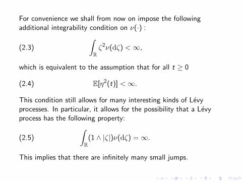
For convenience we shall from now on impose the followingadditional integrability condition on ν(·) :∫

Rζ2ν(dζ) <∞,(2.3)

which is equivalent to the assumption that for all t ≥ 0

E[η2(t)] <∞.(2.4)

This condition still allows for many interesting kinds of Levyprocesses. In particular, it allows for the possibility that a Levyprocess has the following property:∫

R(1 ∧ |ζ|)ν(dζ) =∞.(2.5)

This implies that there are infinitely many small jumps.

Under the assumption (2.3) above the Ito-Levy decompositiontheorem states that any Levy process has the form

η(t) = at + bB(t) +

∫ t

0

∫RζN(ds,dζ),(2.6)

where B(t) is a Brownian motion, and a, b are constants.

More generally, we study the Ito-Levy processes, which are theprocesses of the form

X (t) = x +

∫ t

0α(s, ω)ds +

∫ t

0β(s, ω)dB(s)(2.7)

+

∫ t

0

∫Rγ(s, ζ, ω)N(ds,dζ),

where∫ t

0 |α(s)|ds +∫ t

0 β2(s)ds +

∫ t0

∫R γ

2(s, ζ)ν(dζ)ds <∞ a.s.,and α(t), β(t), and γ(t, ζ) are predictable processes (predictablew.r.t. the filtration Ft generated by η(s), for s ≤ t).

In differential form we have

dX (t) = α(t)dt + β(t)dB(t) +

∫Rγ(t, ζ)N(dt, dζ).(2.8)

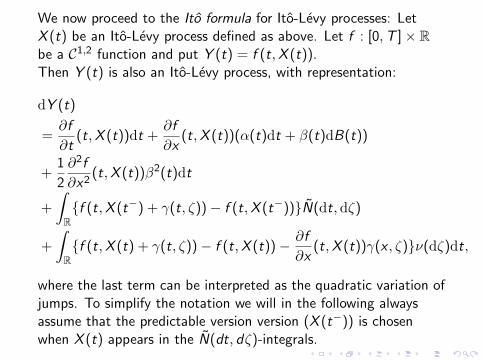
We now proceed to the Ito formula for Ito-Levy processes: LetX (t) be an Ito-Levy process defined as above. Let f : [0,T ]× Rbe a C1,2 function and put Y (t) = f (t,X (t)).Then Y (t) is also an Ito-Levy process, with representation:

dY (t)

=∂f

∂t(t,X (t))dt +

∂f

∂x(t,X (t))(α(t)dt + β(t)dB(t))

+1

2

∂2f

∂x2(t,X (t))β2(t)dt

+

∫Rf (t,X (t−) + γ(t, ζ))− f (t,X (t−))N(dt,dζ)

+

∫Rf (t,X (t) + γ(t, ζ))− f (t,X (t))− ∂f

∂x(t,X (t))γ(x , ζ)ν(dζ)dt,

where the last term can be interpreted as the quadratic variation ofjumps. To simplify the notation we will in the following alwaysassume that the predictable version version (X (t−)) is chosenwhen X (t) appears in the N(dt, dζ)-integrals.

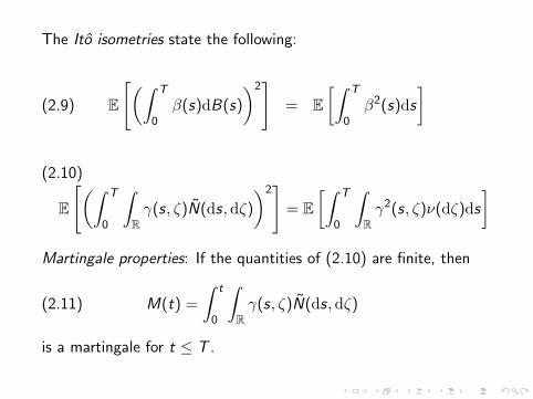
The Ito isometries state the following:

E

[(∫ T

0β(s)dB(s)

)2]

= E[∫ T

0β2(s)ds

](2.9)

E

[(∫ T

0

∫Rγ(s, ζ)N(ds, dζ)

)2]

= E[∫ T

0

∫Rγ2(s, ζ)ν(dζ)ds

](2.10)

Martingale properties: If the quantities of (2.10) are finite, then

M(t) =

∫ t

0

∫Rγ(s, ζ)N(ds, dζ)(2.11)

is a martingale for t ≤ T .

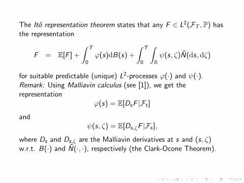
The Ito representation theorem states that any F ∈ L2(FT ,P) hasthe representation

F = E[F ] +

∫ T

0ϕ(s)dB(s) +

∫ T

0

∫Rψ(s, ζ)N(ds,dζ)

for suitable predictable (unique) L2-processes ϕ(·) and ψ(·).Remark: Using Malliavin calculus (see [1]), we get therepresentation

ϕ(s) = E[DsF |Ft ]

andψ(s, ζ) = E[Ds,ζF |Fs ],

where Ds and Ds,ζ are the Malliavin derivatives at s and (s, ζ)w.r.t. B(·) and N(·, ·), respectively (the Clark-Ocone Theorem).

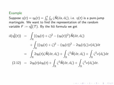
Example

Suppose η(t) = η0(t) =∫ t

0

∫R ζN(ds, dζ), i.e. η(t) is a pure-jump

martingale. We want to find the representation of the randomvariable F := η2

0(T ). By the Ito formula we get

d(η20(t)) =

∫R(η0(t) + ζ)2 − (η0(t))2N(dt, dζ)

+

∫R(η0(t) + ζ)2 − (η0(t))2 − 2η0(t)ζν(dζ)dt

=

∫R

2η0(t)ζN(dt, dζ) +

∫Rζ2N(dt,dζ) +

∫Rζ2ν(dζ)dt

= 2η0(t)dη0(t) +

∫Rζ2N(dt,dζ) +

∫Rζ2ν(dζ)dt.(2.12)

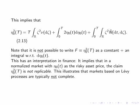
This implies that

η20(T ) = T

∫Rζ2ν(dζ) +

∫ T

02η0(t)dη0(t) +

∫ T

0

∫Rζ2N(dt, dζ).

(2.13)

Note that it is not possible to write F ≡ η20(T ) as a constant + an

integral w.r.t. dη0(t).This has an interpretation in finance: It implies that in anormalized market with η0(t) as the risky asset price, the claimη2

0(T ) is not replicable. This illustrates that markets based on Levyprocesses are typically not complete.

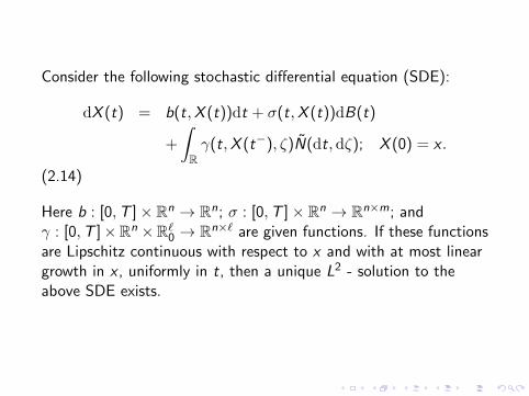
Consider the following stochastic differential equation (SDE):

dX (t) = b(t,X (t))dt + σ(t,X (t))dB(t)

+

∫Rγ(t,X (t−), ζ)N(dt, dζ); X (0) = x .

(2.14)

Here b : [0,T ]× Rn → Rn; σ : [0,T ]× Rn → Rn×m; andγ : [0,T ]×Rn ×R`0 → Rn×` are given functions. If these functionsare Lipschitz continuous with respect to x and with at most lineargrowth in x , uniformly in t, then a unique L2 - solution to theabove SDE exists.

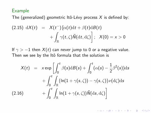
Example

The (generalized) geometric Ito-Levy process X is defined by:

dX (t) = X (t−) [α(t)dt + β(t)dB(t)(2.15)

+

∫Rγ(t, ζ)N(dt,dζ)

]; X (0) = x > 0

If γ > −1 then X (t) can never jump to 0 or a negative value.Then we see by the Ito formula that the solution is

X (t) = x exp

[∫ t

0β(s)dB(s) +

∫ t

0(α(s)− 1

2β2(s))ds

+

∫ t

0

∫Rln(1 + γ(s, ζ))− γ(s, ζ)ν(dζ)ds

+

∫ t

0

∫R

ln(1 + γ(s, ζ))N(ds, dζ)

](2.16)

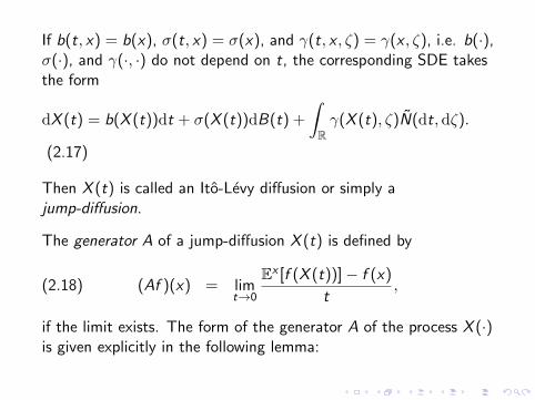
If b(t, x) = b(x), σ(t, x) = σ(x), and γ(t, x , ζ) = γ(x , ζ), i.e. b(·),σ(·), and γ(·, ·) do not depend on t, the corresponding SDE takesthe form

dX (t) = b(X (t))dt + σ(X (t))dB(t) +

∫Rγ(X (t), ζ)N(dt, dζ).

(2.17)

Then X (t) is called an Ito-Levy diffusion or simply ajump-diffusion.

The generator A of a jump-diffusion X (t) is defined by

(Af )(x) = limt→0

Ex [f (X (t))]− f (x)

t,(2.18)

if the limit exists. The form of the generator A of the process X (·)is given explicitly in the following lemma:

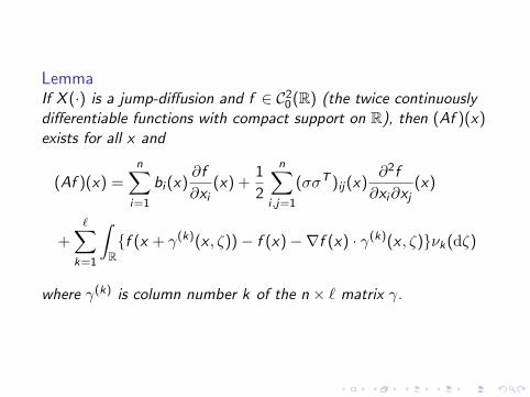
LemmaIf X (·) is a jump-diffusion and f ∈ C2

0(R) (the twice continuouslydifferentiable functions with compact support on R), then (Af )(x)exists for all x and

(Af )(x) =n∑

i=1

bi (x)∂f

∂xi(x) +

1

2

n∑i ,j=1

(σσT )ij(x)∂2f

∂xi∂xj(x)

+∑k=1

∫Rf (x + γ(k)(x , ζ))− f (x)−∇f (x) · γ(k)(x , ζ)νk(dζ)

where γ(k) is column number k of the n × ` matrix γ.

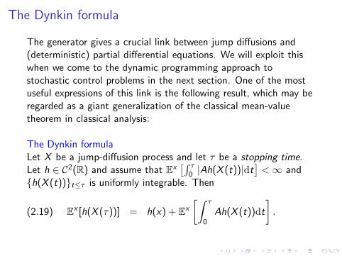
The Dynkin formula

The generator gives a crucial link between jump diffusions and(deterministic) partial differential equations. We will exploit thiswhen we come to the dynamic programming approach tostochastic control problems in the next section. One of the mostuseful expressions of this link is the following result, which may beregarded as a giant generalization of the classical mean-valuetheorem in classical analysis:

The Dynkin formulaLet X be a jump-diffusion process and let τ be a stopping time.Let h ∈ C2(R) and assume that Ex

[∫ τ0 |Ah(X (t))|dt

]<∞ and

h(X (t))t≤τ is uniformly integrable. Then

Ex [h(X (τ))] = h(x) + Ex

[∫ τ

0Ah(X (t))dt

].(2.19)

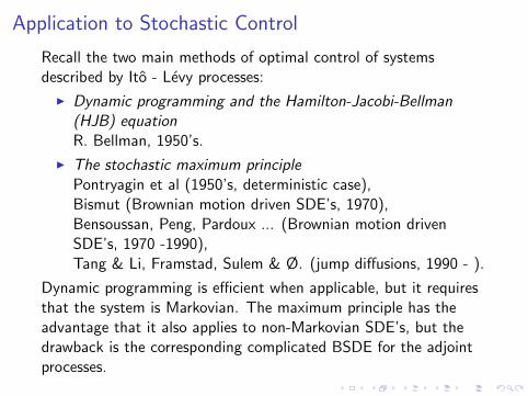
Application to Stochastic Control

Recall the two main methods of optimal control of systemsdescribed by Ito - Levy processes:

I Dynamic programming and the Hamilton-Jacobi-Bellman(HJB) equationR. Bellman, 1950’s.

I The stochastic maximum principlePontryagin et al (1950’s, deterministic case),Bismut (Brownian motion driven SDE’s, 1970),Bensoussan, Peng, Pardoux ... (Brownian motion drivenSDE’s, 1970 -1990),Tang & Li, Framstad, Sulem & Ø. (jump diffusions, 1990 - ).

Dynamic programming is efficient when applicable, but it requiresthat the system is Markovian. The maximum principle has theadvantage that it also applies to non-Markovian SDE’s, but thedrawback is the corresponding complicated BSDE for the adjointprocesses.

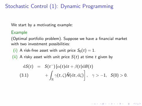
Stochastic Control (1): Dynamic Programming

We start by a motivating example:

Example

(Optimal portfolio problem). Suppose we have a financial marketwith two investment possibilities:

(i) A risk-free asset with unit price S0(t) = 1.

(ii) A risky asset with unit price S(t) at time t given by

dS(t) = S(t−) [α(t)dt + β(t)dB(t)

+

∫Rγ(t, ζ)N(dt,dζ)

], γ > −1, S(0) > 0.(3.1)

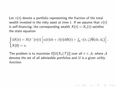
Let π(t) denote a portfolio representing the fraction of the totalwealth invested in the risky asset at time t. If we assume that π(t)is self-financing, the corresponding wealth X (t) = Xπ(t) satisfiesthe state equationdX (t) = X (t−)π(t)

[α(t)dt + β(t)dB(t) +

∫R γ(t, ζ)N(dt, dζ)

].

X (0) = x .

The problem is to maximize E[U(Xπ(T ))] over all π ∈ A, where Adenotes the set of all admissible portfolios and U is a given utilityfunction.

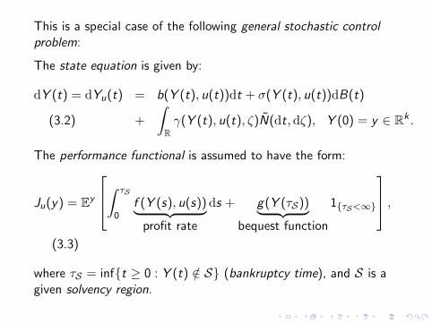
This is a special case of the following general stochastic controlproblem:

The state equation is given by:

dY (t) = dYu(t) = b(Y (t), u(t))dt + σ(Y (t), u(t))dB(t)

+

∫Rγ(Y (t), u(t), ζ)N(dt, dζ), Y (0) = y ∈ Rk .(3.2)

The performance functional is assumed to have the form:

Ju(y) = Ey

∫ τS

0f (Y (s), u(s))︸ ︷︷ ︸

profit rate

ds + g(Y (τS))︸ ︷︷ ︸bequest function

1τS<∞

,(3.3)

where τS = inft ≥ 0 : Y (t) /∈ S (bankruptcy time), and S is agiven solvency region.

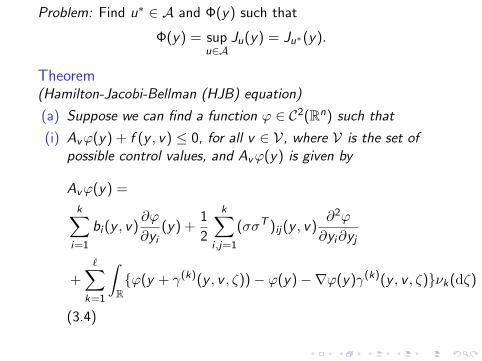
Problem: Find u∗ ∈ A and Φ(y) such that

Φ(y) = supu∈A

Ju(y) = Ju∗(y).

Theorem(Hamilton-Jacobi-Bellman (HJB) equation)

(a) Suppose we can find a function ϕ ∈ C2(Rn) such that

(i) Avϕ(y) + f (y , v) ≤ 0, for all v ∈ V, where V is the set ofpossible control values, and Avϕ(y) is given by

Avϕ(y) =

k∑i=1

bi (y , v)∂ϕ

∂yi(y) +

1

2

k∑i ,j=1

(σσT )ij(y , v)∂2ϕ

∂yi∂yj

+∑k=1

∫Rϕ(y + γ(k)(y , v , ζ))− ϕ(y)−∇ϕ(y)γ(k)(y , v , ζ)νk(dζ)

(3.4)

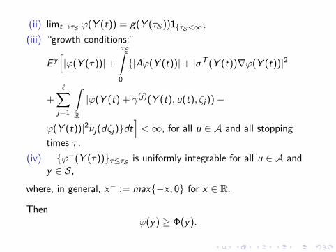
(ii) limt→τS ϕ(Y (t)) = g(Y (τS))1τS<∞

(iii) “growth conditions:”

E y[|ϕ(Y (τ))|+

τS∫0

|Aϕ(Y (t))|+ |σT (Y (t))∇ϕ(Y (t))|2

+∑j=1

∫R

|ϕ(Y (t) + γ(j)(Y (t), u(t), ζj))−

ϕ(Y (t))|2νj(dζj)dt]<∞, for all u ∈ A and all stopping

times τ .

(iv) ϕ−(Y (τ))τ≤τS is uniformly integrable for all u ∈ A andy ∈ S,

where, in general, x− := max−x , 0 for x ∈ R.

Thenϕ(y) ≥ Φ(y).

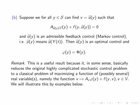
(b) Suppose we for all y ∈ S can find v = u(y) such that

Au(y)ϕ(y) + f (y , u(y)) = 0

and u(y) is an admissible feedback control (Markov control),i.e. u(y) means u(Y (t)). Then u(y) is an optimal control and

ϕ(y) = Φ(y).

Remark. This is a useful result because it, in some sense, basicallyreduces the original highly complicated stochastic control problemto a classical problem of maximizing a function of (possibly several)real variable(s), namely the function v 7→ Avϕ(y) + f (y , v); v ∈ V.We will illustrate this by examples below.

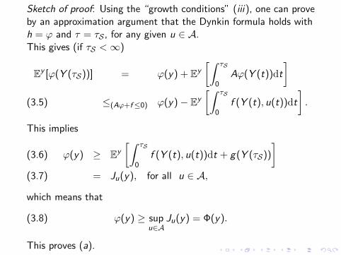
Sketch of proof: Using the “growth conditions” (iii), one can proveby an approximation argument that the Dynkin formula holds withh = ϕ and τ = τS , for any given u ∈ A.This gives (if τS <∞)

Ey [ϕ(Y (τS))] = ϕ(y) + Ey

[∫ τS

0Aϕ(Y (t))dt

]≤(Aϕ+f≤0) ϕ(y)− Ey

[∫ τS

0f (Y (t), u(t))dt

].(3.5)

This implies

ϕ(y) ≥ Ey

[∫ τS

0f (Y (t), u(t))dt + g(Y (τS))

](3.6)

= Ju(y), for all u ∈ A,(3.7)

which means that

(3.8) ϕ(y) ≥ supu∈A

Ju(y) = Φ(y).

This proves (a).

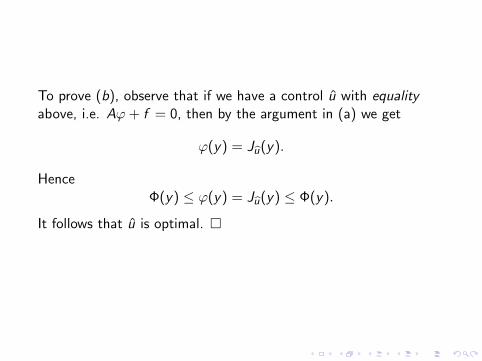
To prove (b), observe that if we have a control u with equalityabove, i.e. Aϕ+ f = 0, then by the argument in (a) we get

ϕ(y) = Ju(y).

HenceΦ(y) ≤ ϕ(y) = Ju(y) ≤ Φ(y).

It follows that u is optimal.

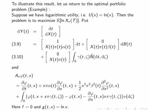
To illustrate this result, let us return to the optimal portfolioproblem (Example) :Suppose we have logarithmic utility, i.e. U(x) = ln(x). Then theproblem is to maximize E[lnXπ(T )]. Put

dY (t) =

[dt

dX (t)

]=

[1

X (t)π(t)α(t)

]dt +

[0

X (t)π(t)β(t)

]dB(t)(3.9)

+

[0

X (t)π(t)

] ∫Rγ(t, ζ)N(dt, dζ)(3.10)

and

Aπϕ(t, x)

=∂ϕ

∂t(t, x) + xπα(t)

∂ϕ

∂x(t, x) +

1

2x2π2β2(t)

∂2ϕ

∂x2(t, x)

+

∫Rϕ(t, x + xπγ(t, ζ))− ϕ(t, x)− ∂ϕ

∂x(t, x)xπγ(t, ζ)ν(dζ)

Here f = 0 and g(t, x) = ln x .

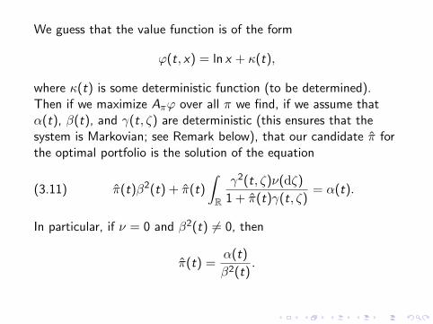
We guess that the value function is of the form

ϕ(t, x) = ln x + κ(t),

where κ(t) is some deterministic function (to be determined).Then if we maximize Aπϕ over all π we find, if we assume thatα(t), β(t), and γ(t, ζ) are deterministic (this ensures that thesystem is Markovian; see Remark below), that our candidate π forthe optimal portfolio is the solution of the equation

(3.11) π(t)β2(t) + π(t)

∫R

γ2(t, ζ)ν(dζ)

1 + π(t)γ(t, ζ)= α(t).

In particular, if ν = 0 and β2(t) 6= 0, then

π(t) =α(t)

β2(t).

We can now proceed to find κ(t), and then verify that with thischoice of ϕ and π all the conditions of the HJB equation. Thus wecan conclude that

π∗(t) := π(t)

is indeed the optimal portfolio.

Remark. The assumption that α(t), β(t), and γ(t, ζ) aredeterministic functions is used when applying the dynamicprogramming techniques in solving this type of stochastic controlproblems. More generally, for the dynamic programming/HJBmethod to work it is necessary that the system is Markovian, i.e.that the coefficients are deterministic functions of t and X (t).This is a limitation of the dynamic programming approach tosolving stochastic control problems.In Section 5 we shall see that there is an alternative approach tostochastic control, called the maximum principle, which does notrequire that the system is Markovian.

Risk minimization

Let p ∈ [1,∞]. A convex risk measure is a map ρ : Lp(FT )→ Rwith the following properties:

(i) (Convexity): ρ(λF + (1− λ)G ) ≤ λρ(F ) + (1− λ)ρ(G ); forall F ,G ∈ Lp(FT ),i.e. diversification reduces the risk.

(ii) (Monotonicity): F ≤ G ⇒ ρ(F ) ≥ ρ(G ); for allF ,G ∈ Lp(FT ),i.e. smaller wealth has bigger risk.

(iii) (Translation invariance): ρ(F + α) = ρ(F )− α if a ∈ R;for all F ∈ Lp(FT ),i.e. adding a constant to F reduces the risk accordingly.

Remark. We may regard ρ(F ) as the amount we need to add tothe position F in order to make it “acceptable”, i.e.ρ(F + ρ(F )) = 0. (F is acceptable if ρ(F ) ≤ 0).

One can prove that basically any risk convex measure ρ can berepresented as follows:

ρ(F ) = supQ∈℘EQ(−F )− ζ(Q)

for some family ℘ of measures Q P and for some convex penaltyfunction ζ : ℘→ R. We refer to [3] for more information aboutrisk measures.

Returning to the financial market above, suppose we want tominimize the risk of the terminal wealth, rather than maximize theexpected utility. Then the problem is to minimize ρ(Xπ(T )) overall possible admissible portfolios π ∈ A.

Hence we want to solve the problem

(4.1) infπ∈A

(supQ∈℘EQ [−Xπ(T )]− ζ(Q)).

This is an example of a stochastic differential game (of zero-sumtype). Heuristically, this can be interpreted as the problem to findthe best possible π under the worst possible scenario Q.

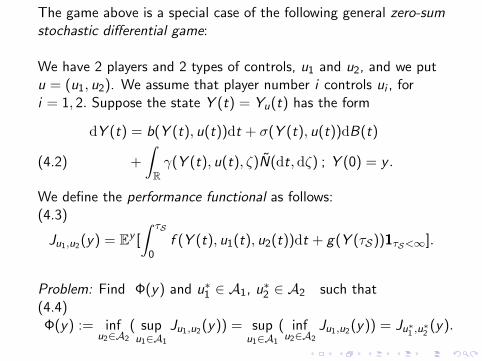
The game above is a special case of the following general zero-sumstochastic differential game:

We have 2 players and 2 types of controls, u1 and u2, and we putu = (u1, u2). We assume that player number i controls ui , fori = 1, 2. Suppose the state Y (t) = Yu(t) has the form

dY (t) = b(Y (t), u(t))dt + σ(Y (t), u(t))dB(t)

+

∫Rγ(Y (t), u(t), ζ)N(dt, dζ) ; Y (0) = y .(4.2)

We define the performance functional as follows:(4.3)

Ju1,u2(y) = Ey [

∫ τS

0f (Y (t), u1(t), u2(t))dt + g(Y (τS))1τS<∞].

Problem: Find Φ(y) and u∗1 ∈ A1, u∗2 ∈ A2 such that(4.4)Φ(y) := inf

u2∈A2

( supu1∈A1

Ju1,u2(y)) = supu1∈A1

( infu2∈A2

Ju1,u2(y)) = Ju∗1 ,u∗2 (y).

The HJBI equation for stochastic differential games

This type of problem is not solvable by the classicalHamilton-Jacobi-Bellman (HJB) equation. We need a new tool,namely the Hamilton-Jacobi-Bellman-Isaacs (HJBI) equation,which in this setting goes as follows:

Theorem(The HJBI equation for zero-sum games ([4]))Suppose we can find a function ϕ ∈ C2(S)

⋂C(S) (continuous up

to the boundary of S) and a Markov control pair (u1(y), u2(y))such that

(i) Au1,u2(y)ϕ(y) + f (y , u1, u2(y)) ≤ 0 ; ∀u1 ∈ A1 and ∀y ∈ S(ii) Au1(y),u2

ϕ(y) + f (y , u1(y), u2) ≥ 0 ; ∀u2 ∈ A2 and ∀y ∈ S(iii) Au1(y),u2(y)ϕ(y) + f (y , u1(y), u2(y)) = 0 ; ∀y ∈ S(iv) lim

t→τSϕ(Yu(t)) = g(Yu(τS))1τS<∞ for all u

(v) “growth conditions”.Then

ϕ(y) = Φ(y) = infu2

(supu1

Ju1,u2(y)) = supu1

(infu2

Ju1,u2(y))

= infu2

Ju1,u2(y) = supu1

Ju1,u2(y)

= Ju1,u2(y).

Proof.The proof is similar to the proof of the HJB equation.

Remark. For the sake of the simplicity of the presentation, in (v)above and also in (iv) of Theorem 10 we choose not to specify therather technical “growth conditions”; we just mention that theyare analogous to the growth conditions in earlier theorems. Werefer to [4] for details. For a specification of the growth conditionsin Theorem 11 we refer to Theorem 2.1 in [9].

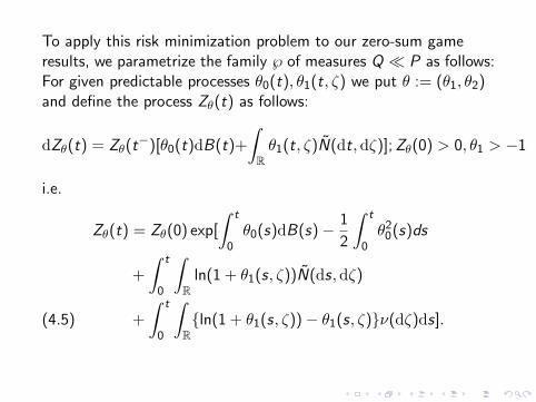
To apply this risk minimization problem to our zero-sum gameresults, we parametrize the family ℘ of measures Q P as follows:For given predictable processes θ0(t), θ1(t, ζ) we put θ := (θ1, θ2)and define the process Zθ(t) as follows:

dZθ(t) = Zθ(t−)[θ0(t)dB(t)+

∫Rθ1(t, ζ)N(dt,dζ)];Zθ(0) > 0, θ1 > −1

i.e.

Zθ(t) = Zθ(0) exp[

∫ t

0θ0(s)dB(s)− 1

2

∫ t

0θ2

0(s)ds

+

∫ t

0

∫R

ln(1 + θ1(s, ζ))N(ds,dζ)

+

∫ t

0

∫Rln(1 + θ1(s, ζ))− θ1(s, ζ)ν(dζ)ds].(4.5)

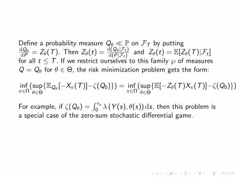
Define a probability measure Qθ P on FT by puttingdQθdP = Zθ(T ). Then Zθ(t) = d(Qθ|Ft)

d(P|Ft)and Zθ(t) = E[Zθ(T )|Ft ]

for all t ≤ T . If we restrict ourselves to this family ℘ of measuresQ = Qθ for θ ∈ Θ, the risk minimization problem gets the form:

infπ∈Π

(supθ∈ΘEQθ

[−Xπ(T )]−ζ(Q0)) = infπ∈Π

(supθ∈ΘE[−Zθ(T )Xπ(T )]−ζ(Q0))

For example, if ζ(Qθ) =∫ τs

0 λ (Y (s), θ(s))ds, then this problem isa special case of the zero-sum stochastic differential game.

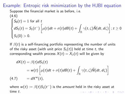
Example: Entropic risk minimization by the HJBI equationSuppose the financial market is as before, i.e.(4.6)

S0(t) = 1 for all t

dS1(t) = S1(t−)

[µ(t)dt + σ(t)dB(t) +

∫Rγ(t, ζ)N(dt, dζ)

]; t ≥ 0

S1(0) > 0.

If β(t) is a self-financing portfolio representing the number of unitsof the risky asset (with unit price S1(t)) held at time t, thecorresponding wealth process X (t) = Xβ(t) will be given by

dX (t) = β(t)dS1(t)

= w(t)

[µ(t)dt + σ(t)dB(t) +

∫Rγ(t, ζ)N(dt, dζ)

]= dXw (t),(4.7)

where w(t) := β(t)S1(t−) is the amount held in the risky asset attime t.

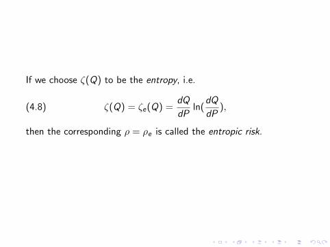
If we choose ζ(Q) to be the entropy, i.e.

(4.8) ζ(Q) = ζe(Q) =dQ

dPln(

dQ

dP),

then the corresponding ρ = ρe is called the entropic risk.

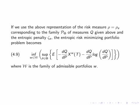
If we use the above representation of the risk measure ρ = ρecorresponding to the family PΘ of measures Q given above andthe entropic penalty ζe , the entropic risk minimizing portfolioproblem becomes

(4.9) infw∈W

(supθ∈Θ

E

[−dQ

dPXw (T )− dQ

dPlog

(dQ

dP

)])where W is the family of admissible portfolios w .

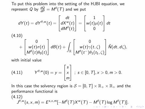
To put this problem into the setting of the HJBI equation, werepresent Q by dQ

dP = Mθ(T ) and we put

dY (t) = dY θ,w (t) =

dtdXw (t)dMθ(t)

=

1w(t)µ(t)

0

dt

+

0w(t)σ(t)Mθ(t)θ0(t)

dB(t) +

∫R

0w(t)γ(t, ζ)

Mθ(t−)θ1(t1, ζ)

N(dt, dζ),

(4.10)

with initial value

(4.11) Y θ,w (0) = y =

sxm

; s ∈ [0,T ], x > 0,m > 0.

In this case the solvency region is S = [0,T ]× R+ × R+ and theperformance functional is(4.12)

Jθ,w (s, x ,m) = E s,x ,m[−Mθ(T )Xw (T )−Mθ(T ) logMθ(T )].

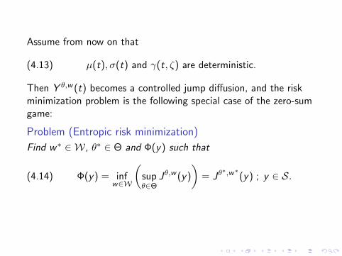
Assume from now on that

(4.13) µ(t), σ(t) and γ(t, ζ) are deterministic.

Then Y θ,w (t) becomes a controlled jump diffusion, and the riskminimization problem is the following special case of the zero-sumgame:

Problem (Entropic risk minimization)

Find w∗ ∈ W, θ∗ ∈ Θ and Φ(y) such that

(4.14) Φ(y) = infw∈W

(supθ∈Θ

Jθ,w (y)

)= Jθ

∗,w∗(y) ; y ∈ S.

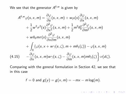
We see that the generator Aθ,w is given by

Aθ,wϕ(s, x ,m) =∂ϕ

∂s(s, x ,m) + wµ(s)

∂ϕ

∂x(s, x ,m)

+1

2w2σ2(s)

∂2ϕ

∂x2(s, x ,m) +

1

2m2θ2

0

∂2ϕ

∂m2(s, x ,m)

+ wθ0mσ(s)∂2ϕ

∂x∂m(s, x ,m)

+

∫Rϕ(s, x + wγ(s, ζ),m + mθ1(ζ))− ϕ(s, x ,m)

−∂ϕ∂x

(s, x ,m)wγ(s, ζ)− ∂ϕ

∂m(s, x ,m)mθ1(ζ)

ν(dζ).(4.15)

Comparing with the general formulation in Section 42, we see thatin this case

f = 0 and g(y) = g(x ,m) = −mx −m log(m).

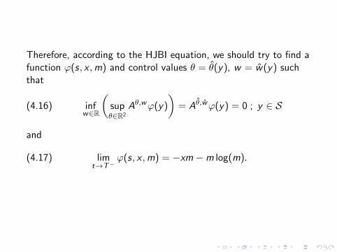
Therefore, according to the HJBI equation, we should try to find afunction ϕ(s, x ,m) and control values θ = θ(y), w = w(y) suchthat

(4.16) infw∈R

(supθ∈R2

Aθ,wϕ(y)

)= Aθ,wϕ(y) = 0 ; y ∈ S

and

(4.17) limt→T−

ϕ(s, x ,m) = −xm −m log(m).

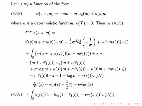
Let us try a function of the form

(4.18) ϕ(s, x ,m) = −xm −m log(m) + κ(s)m

where κ is a deterministic function, κ(T ) = 0. Then by (4.15)

Aθ,wϕ(s, x ,m) =

κ′(s)m + mµ(s)(−m) +1

2m2θ2

0

(− 1

m

)+ wθ0mσ(s)(−1)

+

∫R−(x + wγ(s, ζ))(m + mθ1(ζ)) + xm

− (m + mθ1(ζ)) log(m + mθ1(ζ))

+ m logm + κ(s)(m + mθ1(ζ))− κ(s)m + mwγ(s, ζ)

−mθ1(ζ)(−x − 1− logm + κ(s))ν(dζ)

= m[κ′(s)− wµ(s)− 1

2θ2

0 − wθ0σ(s)

+

∫Rθ1(ζ)1− log(1 + θ1(ζ))− wγ(s, ζ)ν(dζ)](4.19)

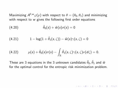
Maximizing Aθ,wϕ(y) with respect to θ = (θ0, θ1) and minimizingwith respect to w gives the following first order equations

(4.20) θ0(s) + w(s)σ(s) = 0

(4.21) 1− log(1 + θ1(s, ζ))− w(s)γ(s, ζ) = 0

(4.22) µ(s) + θ0(s)σ(s)−∫Rθ1(s, ζ)γ(s, ζ)ν(dζ) = 0.

These are 3 equations in the 3 unknown candidates θ0, θ1 and wfor the optimal control for the entropic risk minimization problem.

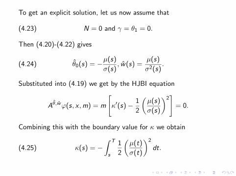
To get an explicit solution, let us now assume that

(4.23) N = 0 and γ = θ1 = 0.

Then (4.20)-(4.22) gives

(4.24) θ0(s) = −µ(s)

σ(s), w(s) =

µ(s)

σ2(s).

Substituted into (4.19) we get by the HJBI equation

Aθ,wϕ(s, x ,m) = m

[κ′(s)− 1

2

(µ(s)

σ(s)

)2]

= 0.

Combining this with the boundary value for κ we obtain

(4.25) κ(s) = −∫ T

s

1

2

(µ(t)

σ(t)

)2

dt.

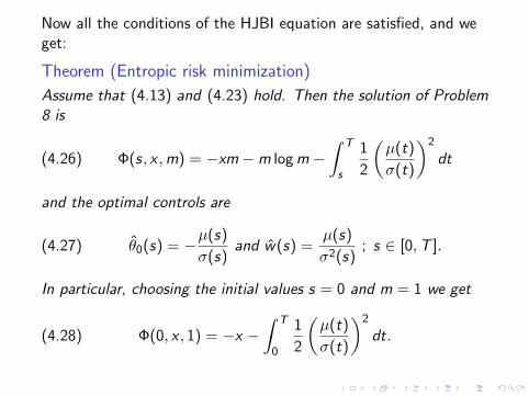
Now all the conditions of the HJBI equation are satisfied, and weget:

Theorem (Entropic risk minimization)

Assume that (4.13) and (4.23) hold. Then the solution of Problem8 is

(4.26) Φ(s, x ,m) = −xm −m logm −∫ T

s

1

2

(µ(t)

σ(t)

)2

dt

and the optimal controls are

(4.27) θ0(s) = −µ(s)

σ(s)and w(s) =

µ(s)

σ2(s); s ∈ [0,T ].

In particular, choosing the initial values s = 0 and m = 1 we get

(4.28) Φ(0, x , 1) = −x −∫ T

0

1

2

(µ(t)

σ(t)

)2

dt.

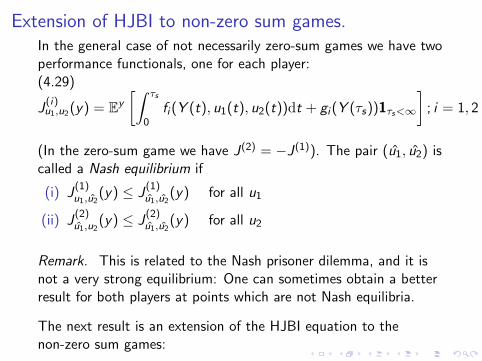
Extension of HJBI to non-zero sum games.In the general case of not necessarily zero-sum games we have twoperformance functionals, one for each player:(4.29)

J(i)u1,u2(y) = Ey

[∫ τs

0fi (Y (t), u1(t), u2(t))dt + gi (Y (τs))1τs<∞

]; i = 1, 2

(In the zero-sum game we have J(2) = −J(1)). The pair (u1, u2) iscalled a Nash equilibrium if

(i) J(1)u1,u2

(y) ≤ J(1)u1,u2

(y) for all u1

(ii) J(2)u1,u2

(y) ≤ J(2)u1,u2

(y) for all u2

Remark. This is related to the Nash prisoner dilemma, and it isnot a very strong equilibrium: One can sometimes obtain a betterresult for both players at points which are not Nash equilibria.

The next result is an extension of the HJBI equation to thenon-zero sum games:

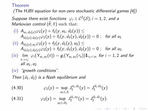
Theorem(The HJBI equation for non-zero stochastic differential games [4])

Suppose there exist functions ϕi ∈ C2(S); i = 1, 2, and aMarkovian control (θ, π) such that:

(i) Au1,u2(y)ϕ1(y) + f1(y , u1, u2(y)) ≤Au1(y),u2(y)ϕ1(y) + f1(y , u1(y), u2(y)) = 0 ; for all u1

(ii) Au1(y),u2ϕ2(y) + f2(y , u1(y), u2) ≤

Au1(y),u2(y)ϕ2(y) + f2(y , u1(y), u2(y)) = 0 ; for all u2.

(iii) limt→τ−s

ϕi (Yu1,u2(t)) = gi (Yu1,u2(τs))1τs<∞ for i = 1, 2 and for

all u1, u2

(iv) “growth conditions”.

Then (u1, u2) is a Nash equilibrium and

ϕ1(y) = supu1∈A

Ju1,u21 (y) = J u1,u2

1 (y)(4.30)

ϕ2(y) = supu2∈A2

J u1,u22 (y) = J u1,u2

2 (y).(4.31)

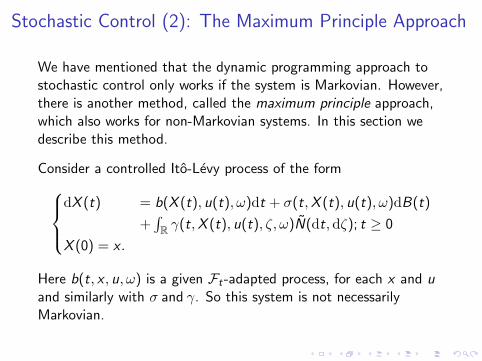
Stochastic Control (2): The Maximum Principle Approach

We have mentioned that the dynamic programming approach tostochastic control only works if the system is Markovian. However,there is another method, called the maximum principle approach,which also works for non-Markovian systems. In this section wedescribe this method.

Consider a controlled Ito-Levy process of the formdX (t) = b(X (t), u(t), ω)dt + σ(t,X (t), u(t), ω)dB(t)

+∫R γ(t,X (t), u(t), ζ, ω)N(dt, dζ); t ≥ 0

X (0) = x .

Here b(t, x , u, ω) is a given Ft-adapted process, for each x and uand similarly with σ and γ. So this system is not necessarilyMarkovian.

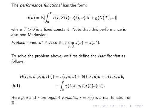
The performance functional has the form:

J(u) = E[

∫ T

0f (t,X (t), u(t), ω)dt + g(X (T ), ω)]

where T > 0 is a fixed constant. Note that this performance isalso non-Markovian.

Problem: Find u∗ ∈ A so that supu∈A

J(u) = J(u∗).

To solve the problem above, we first define the Hamiltonian asfollows:

H(t, x , u, p, q, r(·)) = f (t, x , u) + b(t, x , u)p + σ(t, x , u)q

+

∫Rγ(t, x , u, ζ)r(ζ)ν(dζ).(5.1)

Here p, q and r are adjoint variables, r = r(·) is a real function onR.

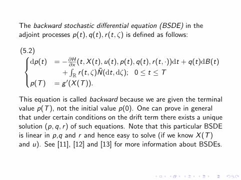
The backward stochastic differential equation (BSDE) in theadjoint processes p(t), q(t), r(t, ζ) is defined as follows:

dp(t) = −∂H

∂x (t,X (t), u(t), p(t), q(t), r(t, ·))dt + q(t)dB(t)

+∫R r(t, ζ)N(dt, dζ); 0 ≤ t ≤ T

p(T ) = g ′(X (T )).

(5.2)

This equation is called backward because we are given the terminalvalue p(T ), not the initial value p(0). One can prove in generalthat under certain conditions on the drift term there exists a uniquesolution (p, q, r) of such equations. Note that this particular BSDEis linear in p,q and r and hence easy to solve (if we know X (T )and u). See [11], [12] and [13] for more information about BSDEs.

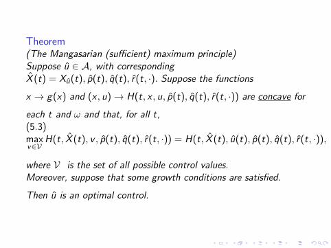
Theorem(The Mangasarian (sufficient) maximum principle)Suppose u ∈ A, with correspondingX (t) = Xu(t), p(t), q(t), r(t, ·). Suppose the functions

x → g(x) and (x , u)→ H(t, x , u, p(t), q(t), r(t, ·)) are concave for

each t and ω and that, for all t,(5.3)maxv∈V

H(t, X (t), v , p(t), q(t), r(t, ·)) = H(t, X (t), u(t), p(t), q(t), r(t, ·)),

where V is the set of all possible control values.Moreover, suppose that some growth conditions are satisfied.

Then u is an optimal control.

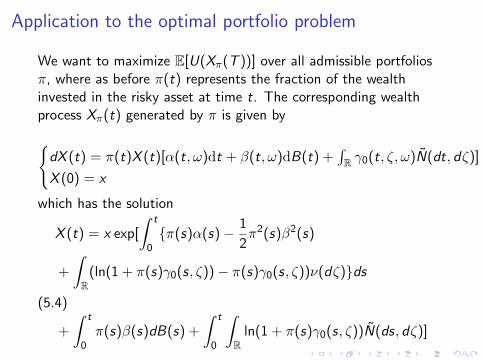
Application to the optimal portfolio problem

We want to maximize E[U(Xπ(T ))] over all admissible portfoliosπ, where as before π(t) represents the fraction of the wealthinvested in the risky asset at time t. The corresponding wealthprocess Xπ(t) generated by π is given bydX (t) = π(t)X (t)[α(t, ω)dt + β(t, ω)dB(t) +

∫R γ0(t, ζ, ω)N(dt, dζ)]

X (0) = x

which has the solution

X (t) = x exp[

∫ t

0π(s)α(s)− 1

2π2(s)β2(s)

+

∫R

(ln(1 + π(s)γ0(s, ζ))− π(s)γ0(s, ζ))ν(dζ)ds

+

∫ t

0π(s)β(s)dB(s) +

∫ t

0

∫R

ln(1 + π(s)γ0(s, ζ))N(ds, dζ)]

(5.4)

In this case the coefficients are

b(t, x , π) = πxα(t),

σ(t, x , π) = πxβ(t),

γ(t, x , π, ζ) = πxγ0(t, ζ),

(5.5)

and the Hamiltonian is

H = πxα(t)p + πxβ(t)q + πx

∫Rγ0(t, ζ)r(ζ)ν(dζ).(5.6)

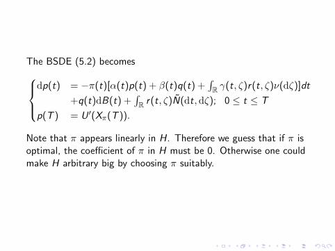
The BSDE (5.2) becomesdp(t) = −π(t)[α(t)p(t) + β(t)q(t) +

∫R γ(t, ζ)r(t, ζ)ν(dζ)]dt

+q(t)dB(t) +∫R r(t, ζ)N(dt, dζ); 0 ≤ t ≤ T

p(T ) = U ′(Xπ(T )).

Note that π appears linearly in H. Therefore we guess that if π isoptimal, the coefficient of π in H must be 0. Otherwise one couldmake H arbitrary big by choosing π suitably.

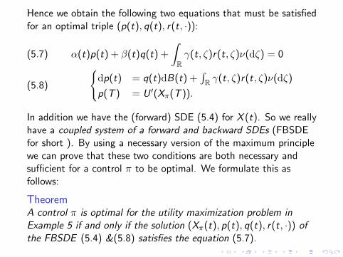
Hence we obtain the following two equations that must be satisfiedfor an optimal triple (p(t), q(t), r(t, ·)):

α(t)p(t) + β(t)q(t) +

∫Rγ(t, ζ)r(t, ζ)ν(dζ) = 0(5.7)

dp(t) = q(t)dB(t) +∫R γ(t, ζ)r(t, ζ)ν(dζ)

p(T ) = U ′(Xπ(T )).(5.8)

In addition we have the (forward) SDE (5.4) for X (t). So we reallyhave a coupled system of a forward and backward SDEs (FBSDEfor short ). By using a necessary version of the maximum principlewe can prove that these two conditions are both necessary andsufficient for a control π to be optimal. We formulate this asfollows:

TheoremA control π is optimal for the utility maximization problem inExample 5 if and only if the solution (Xπ(t), p(t), q(t), r(t, ·)) ofthe FBSDE (5.4) &(5.8) satisfies the equation (5.7).

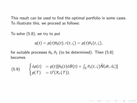
This result can be used to find the optimal portfolio in some cases.To illustrate this, we proceed as follows:

To solve (5.8), we try to put

q(t) = p(t)θ0(t), r(t, ζ) = p(t)θ1(t, ζ),

for suitable processes θ0, θ1 (to be determined). Then (5.8)becomes

dp(t) = p(t)[θ0(t)dB(t) +∫R θ1(t, ζ)N(dt,dζ)]

p(T ) = U ′(Xπ(T )).(5.9)

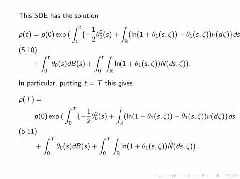
This SDE has the solution

p(t) = p(0) exp( ∫ t

0−1

2θ2

0(s) +

∫R

(ln(1 + θ1(s, ζ))− θ1(s, ζ))ν(dζ)ds

+

∫ t

0θ0(s)dB(s) +

∫ t

0

∫R

ln(1 + θ1(s, ζ))N(ds, ζ)).

(5.10)

In particular, putting t = T this gives

p(T ) =

p(0) exp( ∫ T

0−1

2θ2

0(s) +

∫R

(ln(1 + θ1(s, ζ))− θ1(s, ζ))ν(dζ)ds

+

∫ T

0θ0(s)dB(s) +

∫ T

0

∫R

ln(1 + θ1(s, ζ))N(ds, ζ)).

(5.11)

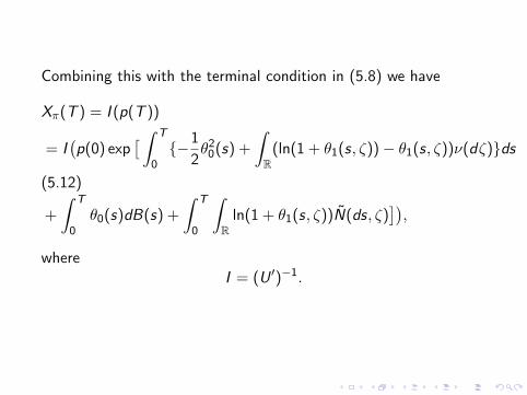
Combining this with the terminal condition in (5.8) we have

Xπ(T ) = I (p(T ))

= I(p(0) exp

[ ∫ T

0−1

2θ2

0(s) +

∫R

(ln(1 + θ1(s, ζ))− θ1(s, ζ))ν(dζ)ds

+

∫ T

0θ0(s)dB(s) +

∫ T

0

∫R

ln(1 + θ1(s, ζ))N(ds, ζ)]),

(5.12)

whereI = (U ′)−1.

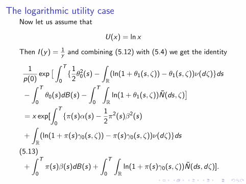
The logarithmic utility caseNow let us assume that

U(x) = ln x

Then I (y) = 1y and combining (5.12) with (5.4) we get the identity

1

p(0)exp

[ ∫ T

01

2θ2

0(s)−∫R

(ln(1 + θ1(s, ζ))− θ1(s, ζ))ν(dζ)ds

−∫ T

0θ0(s)dB(s)−

∫ T

0

∫R

ln(1 + θ1(s, ζ))N(ds, ζ)]

= x exp[

∫ T

0π(s)α(s)− 1

2π2(s)β2(s)

+

∫R

(ln(1 + π(s)γ0(s, ζ))− π(s)γ0(s, ζ))ν(dζ)ds

+

∫ T

0π(s)β(s)dB(s) +

∫ T

0

∫R

ln(1 + π(s)γ0(s, ζ))N(ds, dζ)].

(5.13)

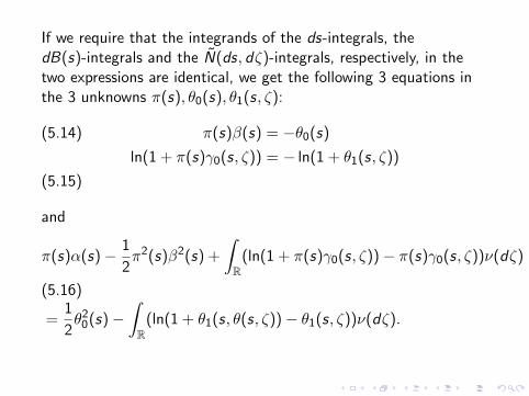
If we require that the integrands of the ds-integrals, thedB(s)-integrals and the N(ds, dζ)-integrals, respectively, in thetwo expressions are identical, we get the following 3 equations inthe 3 unknowns π(s), θ0(s), θ1(s, ζ):

π(s)β(s) = −θ0(s)(5.14)

ln(1 + π(s)γ0(s, ζ)) = − ln(1 + θ1(s, ζ))

(5.15)

and

π(s)α(s)− 1

2π2(s)β2(s) +

∫R

(ln(1 + π(s)γ0(s, ζ))− π(s)γ0(s, ζ))ν(dζ)

=1

2θ2

0(s)−∫R

(ln(1 + θ1(s, θ(s, ζ))− θ1(s, ζ))ν(dζ).

(5.16)

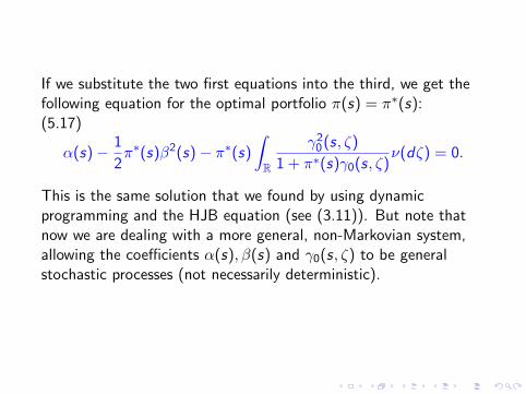
If we substitute the two first equations into the third, we get thefollowing equation for the optimal portfolio π(s) = π∗(s):(5.17)

α(s)− 1

2π∗(s)β2(s)− π∗(s)

∫R

γ20(s, ζ)

1 + π∗(s)γ0(s, ζ)ν(dζ) = 0.

This is the same solution that we found by using dynamicprogramming and the HJB equation (see (3.11)). But note thatnow we are dealing with a more general, non-Markovian system,allowing the coefficients α(s), β(s) and γ0(s, ζ) to be generalstochastic processes (not necessarily deterministic).

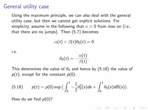
General utility case

Using the maximum principle, we can also deal with the generalutility case, but then we cannot get explicit solutions. Forsimplicity, assume in the following that ν = 0 from now on (i.e.,that there are no jumps). Then (5.7) becomes:

α(t) + β(t)θ0(t) = 0

i.e.

θ0(t) = −α(t)

β(t).

This determines the value of θ0 and hence by (5.18) the value ofp(t), except for the constant p(0):

p(t) = p(0) exp( ∫ t

0−1

2θ2

0(s)ds +

∫ t

0θ0(s)dB(s)

).(5.18)

How do we find p(0)?

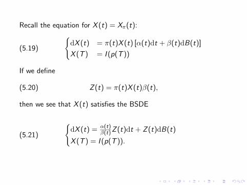
Recall the equation for X (t) = Xπ(t):

(5.19)

dX (t) = π(t)X (t) [α(t)dt + β(t)dB(t)]

X (T ) = I (p(T ))

If we define

(5.20) Z (t) = π(t)X (t)β(t),

then we see that X (t) satisfies the BSDE

(5.21)

dX (t) = α(t)

β(t)Z (t)dt + Z (t)dB(t)

X (T ) = I (p(T )).

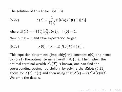
The solution of this linear BSDE is

(5.22) X (t) =1

Γ(t)E [I (p(T ))Γ(T )|Ft ]

where dΓ(t) = −Γ(t)α(t)β(t)dB(t); Γ(0) = 1.

Now put t = 0 and take expectation to get

(5.23) X (0) = x = E [I (p(T ))Γ(T )] .

This equation determines (implicitly) the constant p(0) and henceby (5.21) the optimal terminal wealth Xπ(T ). Then, when theoptimal terminal wealth Xπ(T ) is known, one can find thecorresponding optimal portfolio π by solving the BSDE (5.21)above for X (t),Z (t) and then using that Z (t) = π(t)X (t)β(t).We omit the details.

We have obtained the following:

TheoremThe optimal portfolio π∗ for the general utility and with no jumpsis given by

(5.24) π∗(t) =Z (t)

Xπ∗(t)β(t)

where (Xπ∗(t),Z (t)) solves the BSDE (5.21), with p(0) given by(5.23) and p(T ) given by (5.18).

Remark: The advantage of this approach is that it applies to ageneral non-Markovian setting, which is inaccessible for dynamicprogramming.

Moreover, this approach can be extended to case when the agenthas only partial information to her disposal, which means that herdecisions must be based on an information flow which is asubfiltration of F .

A suitably modified version can also be applied to study optimalcontrol under inside information, i.e. information about the futurevalue of the system.More information can be found in the references below.

Di Nunno, G., Øksendal, B. and Proske, F.: Malliavin Calculusfor Levy Processes with Applications to Finance, SecondEdition, Springer, 2009.

Draouil, O. and Øksendal, B.: A Donsker delta functionalapproach to optimal insider control and applications tofinance. Communications in Mathematics and Statistics(CIMS) 2015 (to appear).

Follmer, H. and Schied, A.: Stochastic Finance, Third Edition,De Gruyter, 2011.

Mataramvura, S. and Øksendal, B.: Risk minimizing portfoliosand HJBI equations for stochastic differential games,Stochastics 80 (2008), 317-337.

Øksendal, B. and Sulem, A.: Applied Stochastic Control ofJump Diffusions, Second Edition, Springer, 2007.

Øksendal, B. and Sulem, A.: Maximum principles for optimalcontrol of forward-backward stochastic differential equations

with jumps, SIAM J. Control Optimization 48 2009),2845-2976.

Øksendal, B. and Sulem, A.: Portfolio optimization undermodel uncertainty and BSDE games, Quantitative Finance 11(2011), 1665-1674.

Øksendal, B. and Sulem, A.: Forward-backward SDE gamesand stochastic control under model uncertainty, J.Optimization Theory and Applications (2012), DOI:10.1007/s10957-012-0166-7.Preprint, University of Oslo2011:12(https://www.duo.uio.no/handle/10852/10436)

Øksendal, B. and Sulem, A.: Risk minimization in financialmarkets modeled by Ito-Levy processes,(2014), arXiv1402.3131. Afrika Matematika.

Peng, S. and Pardoux, E.: Adapted solution of a backwardstochastic differential equation, Systems and Control Letters14 (1990), 55-61.

Quenez, M.-C.: Backward Stochastic Differential Equations,Encyclopedia of Quantitative Finance (2010), 134-145.

Quenez, M.-C. and Sulem, A.: BSDEs with jumps,optimization and applications to dynamic risk measures,Stoch. Proc. and Their Appl. 123 (2013), 3328-3357.

Royer, M.: Backward stochastic differential equations withjumps and related non-linear expectations, Stoch. Proc. andTheir Appl. 116 (2006), 1358-1376.

Tang, S. and Li, X.: Necessary conditions for optimal controlof stochastic systems with random jumps, SIAM J. ControlOptimization. 32 (1994), 1447-1475.