Embed Size (px)
Citation preview

STUDENT MATHEMAT ICAL L IBRARY Volume 87
An Introduction to Ramsey Theory
Fast Functions, Infinity, and Metamathematics
Matthew Katz
Jan Reimann
Mathematics Advanced Study Semesters

An Introduction to Ramsey Theory

STUDENT MATHEMAT ICAL L IBRARYVolume 87
An Introduction to Ramsey TheoryFast Functions, Infinity, and Metamathematics
Matthew Katz
Jan Reimann
Mathematics Advanced Study Semesters

Editorial Board
Satyan L. DevadossRosa Orellana
John Stillwell (Chair)Serge Tabachnikov
2010 Mathematics Subject Classification. Primary 05D10,03-01, 03E10, 03B10, 03B25, 03D20, 03H15.
Jan Reimann was partially supported by NSF Grant DMS-1201263.
For additional information and updates on this book, visitwww.ams.org/bookpages/stml-87
Library of Congress Cataloging-in-Publication Data
Names: Katz, Matthew, 1986– author. | Reimann, Jan, 1971– author. | PennsylvaniaState University. Mathematics Advanced Study Semesters.Title: An introduction to Ramsey theory: Fast functions, infinity, and metamathemat-ics / Matthew Katz, Jan Reimann.Description: Providence, Rhode Island: American Mathematical Society, [2018] |Series: Student mathematical library; 87 | “Mathematics Advanced Study Semesters.”| Includes bibliographical references and index.Identifiers: LCCN 2018024651 | ISBN 9781470442903 (alk. paper)Subjects: LCSH: Ramsey theory. | Combinatorial analysis. | AMS: Combinatorics –Extremal combinatorics – Ramsey theory. msc | Mathematical logic and foundations– Instructional exposition (textbooks, tutorial papers, etc.). msc | Mathematical logicand foundations – Set theory – Ordinal and cardinal numbers. msc | Mathematicallogic and foundations – General logic – Classical first-order logic. msc | Mathematicallogic and foundations – General logic – Decidability of theories and sets of sentences.msc | Mathematical logic and foundations – Computability and recursion theory –Recursive functions and relations, subrecursive hierarchies. msc | Mathematical logicand foundations – Nonstandard models – Nonstandard models of arithmetic. mscClassification: LCC QA165 .K38 2018 | DDC 511/.66–dc23LC record available at https://lccn.loc.gov/2018024651
Copying and reprinting. Individual readers of this publication, and nonprofit li-braries acting for them, are permitted to make fair use of the material, such as tocopy select pages for use in teaching or research. Permission is granted to quote briefpassages from this publication in reviews, provided the customary acknowledgment ofthe source is given.
Republication, systematic copying, or multiple reproduction of any material in thispublication is permitted only under license from the American Mathematical Society.Requests for permission to reuse portions of AMS publication content are handledby the Copyright Clearance Center. For more information, please visit www.ams.org/
publications/pubpermissions.Send requests for translation rights and licensed reprints to reprint-permission
@ams.org.
c©2018 by the authors. All rights reserved.Printed in the United States of America.
©∞ The paper used in this book is acid-free and falls within the guidelinesestablished to ensure permanence and durability.
Visit the AMS home page at https://www.ams.org/
10 9 8 7 6 5 4 3 2 1 23 22 21 20 19 18

Contents
Foreword: MASS at Penn State University vii
Preface ix
Chapter 1. Graph Ramsey theory 1
§1.1. The basic setting 1
§1.2. The basics of graph theory 4
§1.3. Ramsey’s theorem for graphs 14
§1.4. Ramsey numbers and the probabilistic method 21
§1.5. Turan’s theorem 31
§1.6. The finite Ramsey theorem 34
Chapter 2. Infinite Ramsey theory 41
§2.1. The infinite Ramsey theorem 41
§2.2. Konig’s lemma and compactness 43
§2.3. Some topology 50
§2.4. Ordinals, well-orderings, and the axiom of choice 55
§2.5. Cardinality and cardinal numbers 64
§2.6. Ramsey theorems for uncountable cardinals 70
§2.7. Large cardinals and Ramsey cardinals 80
v

vi Contents
Chapter 3. Growth of Ramsey functions 85
§3.1. Van der Waerden’s theorem 85
§3.2. Growth of van der Waerden bounds 98
§3.3. Hierarchies of growth 105
§3.4. The Hales-Jewett theorem 113
§3.5. A really fast-growing Ramsey function 123
Chapter 4. Metamathematics 129
§4.1. Proof and truth 129
§4.2. Non-standard models of Peano arithmetic 145
§4.3. Ramsey theory in Peano arithmetic 152
§4.4. Incompleteness 159
§4.5. Indiscernibles 171
§4.6. Diagonal indiscernibles via Ramsey theory 182
§4.7. The Paris-Harrington theorem 188
§4.8. More incompleteness 193
Bibliography 199
Notation 203
Index 205

Foreword: MASS atPenn State University
This book is part of a collection published jointly by the American
Mathematical Society and the MASS (Mathematics Advanced Study
Semesters) program as a part of the Student Mathematical Library
series. The books in the collection are based on lecture notes for
advanced undergraduate topics courses taught at the MASS (Math-
ematics Advanced Study Semesters) program at Penn State. Each
book presents a self-contained exposition of a non-standard mathe-
matical topic, often related to current research areas, which is acces-
sible to undergraduate students familiar with an equivalent of two
years of standard college mathematics, and is suitable as a text for
an upper division undergraduate course.
Started in 1996, MASS is a semester-long program for advanced
undergraduate students from across the USA. The program’s curricu-
lum amounts to sixteen credit hours. It includes three core courses
from the general areas of algebra/number theory, geometry/topol-
ogy, and analysis/dynamical systems, custom designed every year; an
interdisciplinary seminar; and a special colloquium. In addition, ev-
ery participant completes three research projects, one for each core
course. The participants are fully immersed into mathematics, and
this, as well as intensive interaction among the students, usually leads
vii

viii Foreword: MASS at Penn State University
to a dramatic increase in their mathematical enthusiasm and achieve-
ment. The program is unique for its kind in the United States.
Detailed information about the MASS program at Penn State can
be found on the website www.math.psu.edu/mass.
Preface
If we split a set into two parts, will at least one of the parts behave like
the whole? Certainly not in every aspect. But if we are interested only
in the persistence of certain small regular substructures, the answer
turns out to be “yes”.
A famous example is the persistence of arithmetic progressions.
The numbers 1, 2, . . . ,N form the most simple arithmetic progres-
sion imaginable: The next number differs from the previous one by
exactly 1. But the numbers 4, 7, 10, 13, . . . also form an arithmetic
progression, where each number differs from its predecessor by 3.
So, if we split the set {1, . . . ,N} into two parts, will one of them
contain an arithmetic progression, say of length 7? Van der Waerden’s
theorem, one of the central results of Ramsey theory, tells us precisely
that: For every k there exists a number N such that if we split the
set {1, . . . ,N} into two parts, one of the parts contains an arithmetic
progression of length k.
Van der Waerden’s theorem exhibits the two phenomena, the
interplay of which is at the heart of Ramsey theory:
● Principle 1: If we split a large enough object with a certain
regularity property (such as a set containing a long arith-
metic progression) into two parts, one of the parts will also
exhibit this property (to a certain degree).
ix

x Preface
● Principle 2: When proving Principle 1, “large enough”
often means very, very, very large.
The largeness of the numbers encountered seems intrinsic to Ram-
sey theory and is one of its most peculiar and challenging features.
Many great results in Ramsey theory are actually new proofs of known
results, but the new proofs yield much better bounds on how large an
object has to be in order for a Ramsey-type persistence under parti-
tions to take place. Sometimes, “large enough” is even so large that
the numbers become difficult to describe using axiomatic arithmetic—
so large that they venture into the realm of metamathematics.
One of the central issues of metamathematics is provability. Sup-
pose we have a set of axioms, such as the group axioms or the ax-
ioms for a vector space. When you open a textbook on group theory
or linear algebra, you will find results (theorems) that follow from
these axioms by means of logical deduction. But how does one know
whether a certain statement about groups is provable (or refutable)
from the axioms at all? A famous instance of this problem is Euclid’s
fifth postulate (axiom), also known as the parallel postulate. For more
than two thousand years, mathematicians tried to derive the parallel
postulate from the first four postulates. In the 19th century it was fi-
nally discovered that the parallel postulate is independent of the first
four axioms, that is, neither the postulate nor its negation is entailed
by the first four postulates.
Toward the end of the 19th century, mathematicians became in-
creasingly disturbed as more and more strange and paradoxical re-
sults appeared. There were different sizes of infinity, one-dimensional
curves that completely fill two-dimensional regions, and subsets of the
real number line that have no reasonable measure of length, or there
was the paradox of a set containing all sets not containing them-
selves. It seemed increasingly important to lay a solid foundation
for mathematics. David Hilbert was one of the foremost leaders of
this movement. He suggested finding axiom systems from which all
of mathematics could be formally derived and in which it would be
impossible to derive any logical inconsistencies.
An important part of any such foundation would be axioms which
describe the natural numbers and the basic operations we perform on

Preface xi
them, addition and multiplication. In 1931, Kurt Godel published
his famous incompleteness theorems, which dealt a severe blow to
Hilbert’s program: For any reasonable, consistent axiomatization of
arithmetic, there are independent statements—statements which can
be neither proved nor refuted from the axioms.
The independent statements that Godel’s proof produces, how-
ever, are of a rather artificial nature. In 1977, Paris and Harrington
found a result in Ramsey theory that is independent of arithmetic.
In fact, their theorem is a seemingly small variation of the original
Ramsey theorem. It is precisely the very rapid growth of the Ram-
sey numbers (recall Principle 2 above) associated with this variation
of Ramsey’s theorem that makes the theorem unprovable in Peano
arithmetic.
But if the Paris-Harrington principle is unprovable in arithmetic,
how do we convince ourselves that it is true? We have to pass from
the finite to the infinite. Van der Waerden’s theorem above is of a
finitary nature: All sets, objects, and numbers involved are finite.
However, basic Ramsey phenomena also manifest themselves when
we look at infinite sets, graphs, and so on. Infinite Ramsey theo-
rems in turn can be used (and, as the result by Paris and Harrington
shows, sometimes have to be used) to deduce finite versions using
the compactness principle, a special instance of topological compact-
ness. If we are considering only the infinite as opposed to the finite,
Principle 2 in many cases no longer applies.
● Principle 1 (infinite version): If we split an infinite ob-
ject with a certain regularity property (such as a set contain-
ing arbitrarily long arithmetic progressions) into two parts,
one infinite part will exhibit this property, too.
If we take into account, on the other hand, that there are differ-
ent sizes of infinity, as reflected by Cantor’s theory of ordinals and
cardinals, Principle 2 reappears in a very interesting way. Moreover,
as with the Paris-Harrington theorem, it leads to metamathematical
issues, this time in set theory.

xii Preface
It is the main goal of this book to introduce the reader to the
interplay between Principles 1 and 2, from finite combinatorics to set
theory to metamathematics. The book is structured as follows.
In Chapter 1, we prove Ramsey’s theorem and study Ramsey
numbers and how large they can be. We will make use of the proba-
bilistic methods of Paul Erdos to give lower bounds for the Ramsey
numbers and a result in extremal graph theory.
In Chapter 2, we prove an infinite version of Ramsey’s theorem
and describe how theorems about infinite sets can be used to prove
theorems about finite sets via compactness arguments. We will use
such a strategy to give a new proof of Ramsey’s theorem. We also
connect these arguments to topological compactness. We introduce
ordinal and cardinal numbers and consider generalizations of Ram-
sey’s theorem to uncountable cardinals.
Chapter 3 investigates other classical Ramsey-type problems and
the large numbers involved. We will encounter fast-growing functions
and make an analysis of these in the context of primitive recursive
functions and the Grzegorczyk hierarchy. Shelah’s elegant proof of
the Hales-Jewett theorem, and a Ramsey-type theorem with truly
explosive bounds due to Paris and Harrington, close out the chapter.
Chapter 4 deals with metamathematical aspects. We introduce
basic concepts of mathematical logic such as proof and truth, and we
discuss Godel’s completeness and incompleteness theorems. A large
part of the chapter is dedicated to formulating and proving the Paris-
Harrington theorem.
The results covered in this book are all cornerstones of Ramsey
theory, but they represent only a small fraction of this fast-growing
field. Many important results are only briefly mentioned or not ad-
dressed at all. The same applies to important developments such as
ultrafilters, structural Ramsey theory, and the connection with dy-
namical systems. This is done in favor of providing a more complete
narrative explaining and connecting the results.
The unsurpassed classic on Ramsey theory by Graham, Roth-
schild, and Spencer [24] covers a tremendous variety of results. For
those especially interested in Ramsey theory on the integers, the book

Preface xiii
by Landman and Robertson [43] is a rich source. Other reading sug-
gestions are given throughout the text.
The text should be accessible to anyone who has completed a
first set of proof-based math courses, such as abstract algebra and
analysis. In particular, no prior knowledge of mathematical logic
is required. The material is therefore presented rather informally
at times, especially in Chapters 2 and 4. The reader may wish to
consult a textbook on logic, such as the books by Enderton [13] and
Rautenberg [54], from time to time for more details.
This book grew out of a series of lecture notes for a course on
Ramsey theory taught in the MASS program of the Pennsylvania
State University. It was an intense and rewarding experience, and the
authors hope this book conveys some of the spirit of that semester
back in the fall of 2011.
It seems appropriate to close this introduction with a few words
on the namesake of Ramsey theory. Frank Plumpton Ramsey (1903–
1930) was a British mathematician, economist, and philosopher. A
prodigy in many fields, Ramsey went to study at Trinity College
Cambridge when he was 17 as a student of economist John May-
nard Keynes. There, philosopher Ludwig Wittgenstein also served as
a mentor. Ramsey was largely responsible for Wittgenstein’s Tracta-
tus Logico-Philosophicus being translated into English, and the two
became friends.
Ramsey was drawn to mathematical logic. In 1928, at the age
of 25, Ramsey wrote a paper regarding consistency and decidability.
His paper, On a problem in formal logic, primarily focused on solv-
ing certain problems of axiomatic systems, but in it can be found a
theorem that would become one of the crown jewels of combinatorics.
Given any r, n, and μ we can find an m0 such that, if m ≥ m0
and the r-combinations of any Γm are divided in any manner
into μ mutually exclusive classes Ci (i = 1, 2, . . . , μ), then Γm
must contain a sub-class Δn such that all the r-combinations
of members of Δn belong to the same Ci. [53, Theorem B,
p. 267]

xiv Preface
Ramsey died young, at the age of 26, of complications from
surgery and sadly did not get to see the impact and legacy of his
work.
Acknowledgment. The authors would like to thank Jennifer Chubb
for help with the manuscript and for many suggestions on how to
improve the book.
State College, Pennsylvania Matthew Katz
April 2018 Jan Reimann

Chapter 1
Graph Ramsey theory
1.1. The basic setting
Questions in Ramsey theory come in a specific form: For a desired
property, how large must a finite set be to ensure that if we break up
the set into parts, at least one part exhibits the property?
Definition 1.1. Given a non-empty set S, a finite partition of S is
a collection of subsets S1, . . . , Sr such that the union of the subsets is
S and their pairwise intersections are empty, i.e. each element of S is
in exactly one subset Si.
A set partition is the mathematical way to describe splitting a
larger set up into multiple smaller sets. In studying Ramsey theory,
we often think of a partition as a coloring of the elements where we
distinguish one subset from another by painting all the elements in
each of the subsets Si the same color, each Si having a distinct color.
Of course, the terms “paint” and “color” should be taken ab-
stractly. If we are using two colors, it doesn’t matter if we call our
colors “red” and “blue” or “1” and “2”. To express things mathe-
matically, any finite set of r colors can be identified with the set of
integers [r] ∶= {1, 2, . . . , r}. Therefore, a partition of a set S into r
subsets can be represented by a function c, where
c ∶ S → [r].
1
2 1. Graph Ramsey theory
We will call these functions r-colorings. If we have a subset S′ ⊂ S
whose elements all have the same color, we call that subset monochro-
matic. Equivalently, we can say that a subset S′ is monochromatic
if it is contained entirely within one subset of the set partition, or if
the coloring function c restricted to S′ is constant.
It is using colorings that “Ramsey-type” questions are usually
phrased: How many elements does a set S need so that given any
r-coloring of S (or of collections of subsets of S), we can find a
monochromatic subset of a certain size and with a desired property?
A fundamental example appears in Ramsey’s 1928 paper [53]:
Is there a large enough number of elements a set S needs to
have to guarantee that given any r-coloring on [S]p, the set
of p-element subsets of S, there will exist a monochromatic
subset of size k?
Ramsey showed that the answer is “yes”. We will study this
question throughout this chapter and prove it in full generality in
Section 1.6.
Essential notation. Questions and statements in Ramsey theory
can get somewhat complicated, since they will often involve several
parameters and quantifiers. To help remedy this, a good system of
notation is indispensable. As already mentioned, [S]p denotes the set
of subsets of S of size p, where p ≥ 1, that is,
[S]p = {T ∶ T ⊆ S, ∣T ∣ = p}.
S will often be of the form [n] = {1, . . . , n}, and to increase readability,
we write [n]p for [[n]]p. Note that if ∣S∣ = n, then ∣[S]p∣ = (np
).The arrow notation was introduced by Erdos and Rado [15]. We
write
N �→ (k)prto mean that
if ∣S∣ = N , then every r-coloring of [S]p has a monochromatic
subset of size k.
We will be dealing with colorings of sets of all kinds. For example,
c ∶ [N]3 → {1, 2, 3, 4} means that we have a 4-coloring of the set of

1.1. The basic setting 3
three-element subsets of N. Formally, we would have to write such
functions as c({a1, a2, a3}), but to improve readability, we will use
the notation c(a1, a2, a3) instead.
The pigeonhole principle. The most basic fact about partitions of
sets, as well as a key combinatorial tool, is the pigeonhole principle,
often worded in terms of objects and boxes.
If n objects are put into r boxes where n > r, then at least one
box will contain at least 2 objects.
In arrow notation,
n �→ (2)1r whenever n > r.
The pigeonhole principle seems obvious; if the r boxes have at
most one object, then there can be at most r objects. However, in
its simplicity lies a powerful counting argument which will form the
backbone of many of the arguments in this book. It is believed that
the first time the pigeonhole principle was explicitly formulated was
in 1834 by Dirichlet.1
We can rephrase the pigeonhole principle in terms of set parti-
tions: If a set with n elements is partitioned into r subsets where
n > r, then at least one subset will contain at least 2 elements. From
our point of view, the pigeonhole principle can be seen as the first
Ramsey-type theorem: It asserts the existence of a subset with more
than one element, provided n is “large enough”.
The pigeonhole principle can be strengthened in the following
way:
Theorem 1.2 (Strong pigeonhole principle). If a set with n elements
is partitioned into r subsets, then at least one subset will contain at
least ⌈nr
⌉ elements.
As usual, ⌈nr
⌉ is the least integer greater than or equal to nr.
Again, the proof is clear; if all r subsets have less than ⌈nr
⌉ elements,
then there would be fewer than n elements in the set.
1The pigeonholes in the name of the principle refer to a drawer or shelf of smallholes used for sorting mail, and are only metaphorically related to the homes of rockdoves. It is interesting to note that Dirichlet might have had these sorts of pigeonholesin mind as his father was the postmaster of his city [5].

4 1. Graph Ramsey theory
The strong pigeonhole principle completely answers the Ramsey-
type question, “how large does a set S need to be so that any r-
coloring of S has a monochromatic subset of size at least k?” The
answer is that N must be at least r(k−1) +1, and any smaller would
be too few elements. We can write this result in arrow notation.
Theorem 1.3 (Strong pigeonhole principle, arrow notation).
N �→ (k)1r if and only if N ≥ r(k − 1) + 1.
In this case, we are able to get an exact cut-off of how large the
set needs to be; however, we will see that getting exact answers to
Ramsey-type questions will not always be easy, or even possible.
While the pigeonhole principle is a rather obvious statement in
the finite realm, its infinite versions are not trivial and require the
development of a theory of infinite sizes (cardinalities). We will do
this in Chapter 2.
Exercise 1.4. Prove that any subset of size n + 1 from [2n] must
contain two elements whose sum is 2n + 1.
1.2. The basics of graph theory
We want to move from coloring single elements of sets to coloring
two-element subsets, that is, colorings on [S]2. This is when the true
nature of Ramsey theory starts to emerge.
Thanks to Euler [16], we have a useful geometric representation
for subsets of [S]2: combinatorial graphs. Given a subset of [S]2, foreach element of S you can draw a dot, or vertex, and then connect two
dots by a line segment, or edge, if the pair of corresponding elements
is in your subset. This sort of configuration is called a combinatorial
graph.
For those unfamiliar with graph theory, this section will present
the basic ideas from graph theory that will be needed in this book.
For more background on graph theory, there are a number of excellent
textbooks, such as [4,12].

1.2. The basics of graph theory 5
Definition 1.5. A (combinatorial2) graph is an ordered pair G =(V,E) where V , the vertex set, is any non-empty set and E, the
edge set3, is any subset of [V ]2.
The size of the vertex set is called the order of the graph G and
is denoted by ∣G∣. A graph may be called finite or infinite depending
on the size of its vertex set. In this chapter we will deal exclusively
with finite graphs, those with finite vertex sets. In the next chapter,
we will encounter infinite graphs. Figure 1.1 shows an example of a
finite graph with V = {1, 2, 3, 4, 5}.
1
2
3
4
5
Figure 1.1. A graph with V = {1,2,3,4,5}and E = {{1,2},{1,5},{2,3},{2,4},{3,5}}
The actual elements of the vertex set are often less important than
its cardinality. Whether the vertex set is {1, 2, 3, 4, 5} or {a, b, c, d, e}carries no importance for us, as long as the corresponding graph is
essentially the same. Mathematically, “essentially the same” means
that the two objects are isomorphic. Two graphs G = (V,E) and
G′ = (V ′,E′) are isomorphic, written G ≅ G′, if there is a bijection
2The adjective combinatorial is used to distinguish this type of graph from thegraph of a function. It is usually clear from the context which type of graph is meant,and so we will just speak of “graphs”.
3Note that the definition of the edge set is not standard across all texts. Otherauthors may call the graphs we use simple graphs to emphasize that our edge set doesnot allow multiple edges between vertices or edges which begin and end at the samevertex, while theirs do.

6 1. Graph Ramsey theory
ϕ between V and V ′ such that {v,w} is an edge in E if and only if
{ϕ(v), ϕ(w)} is an edge in E′. In Figure 1.2, we see two isomorphic
graphs. Although they might look rather different at first glance,
mapping 1 ↦ C, 2 ↦ B, 3 ↦ D, and 4 ↦ A transforms the left graph
into the right one.
1
2 3
4
A B
C
D
Figure 1.2. Two isomorphic graphs
We say that two vertices u and v in V are adjacent if {u, v}is in the edge set. In this case, u and v are the endpoints of the
edge. Since our edges are unordered pairs4, adjacency is a symmetric
relationship, that is, if u is adjacent to v, then v is also adjacent to
u.
Given a vertex v of a graph, we define the degree of the vertex as
the number of edges connected to the vertex and denote it by deg(v).In a finite graph, the number of edges will also be finite, and so must
the degree of every vertex. However, in an infinite graph, it is possible
that deg(v) = ∞. In either case, each edge contributes to the degree
of exactly two vertices, and so we get the degree-sum formula:
∑v∈V
deg(v) = 2∣E∣.
We say that two graphs with the same vertex set, G1 = (V,E1)and G2 = (V,E2), are complements if the edge sets E1 and E2 are
complements (as sets) in [V ]2. This means that if G1 and G2 are
4Another possible definition would be that the edge set is a set of ordered pairs.The result would be a graph where each edge has a “direction” associated with it, likea one-way street. Graphs whose edges are ordered pairs are called directed graphs.

1.2. The basics of graph theory 7
complements, then u and v are adjacent in G2 if and only if they are
not adjacent in G1, and vice versa.
1
2 3
4 1
2 3
4
Figure 1.3. The two graphs are complements of each other.
Subgraphs, paths, and connectedness. Intuitively, the concepts
of subgraph and path are easy to describe. If you draw a graph and
then erase some of the vertices and edges, you get a subgraph. If
you start at one vertex in a graph and then “walk” along the edges,
tracing out your motion as you go from vertex to vertex, you have a
path. In both cases, we are talking about restricting the vertex and/or
edge sets of our graphs.
Given a graph G = (V,E), if we choose a subset V ′ of V , we
get a corresponding subset of E consisting of all the edges with both
endpoints in V ′. We call this subset the restriction of E to V ′ and
denote it by E∣V ′ ; formally, E∣V ′ ∶= E ∩ [V ′]2.
Definition 1.6.
(i) Given two graphs G = (V,E) and G′ = (V ′,E′), if V ′ ⊆ V
and E′ ⊆ E∣V ′ , then G′ is a subgraph of G.
(ii) Given a graph G = (V,E), if V ′ ⊆ V , then G∣V ′ ∶= (V ′,E∣V ′)is the subgraph induced by V ′.
Geometrically, an induced subgraph results in choosing a set of
vertices in the graph and then erasing all the other vertices and any
edge whose endpoint is a vertex you just erased.
8 1. Graph Ramsey theory
1
2
3
4
1
2
3
1
2
3
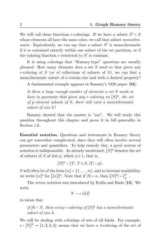
Figure 1.4. A graph G = (V,E) is shown on the left. Themiddle graph is a subgraph of G, but not an induced subgraph,
while the graph on the right is an induced subgraph of G.
Definition 1.7. A path P = (V,E) is any graph (or subgraph) where
V = {x0, x1, . . . , xn} and E = {{x0, x1},{x1, x2}, . . . ,{xn−1, xn}}.
Note that the definition of path requires all vertices xi along the
path to be distinct—along a path, we can visit each vertex only once.
The size of the edge set in a path is called the length of the path. We
allow paths of length 0, which are just single vertices. Rather than as
a graph, we can also think of a path as a finite sequence of vertices
which begin at x0 and end at xn. If n ≥ 2 and x0 and xn are adjacent,
we can extend the path to a cycle or closed path, beginning and
ending at x0.
If there exists a path that begins at vertex u and ends at vertex
v, then we say u and v are connected. Connectedness is a good
example of an equivalence relation:
● it is reflexive—every vertex u is connected to itself (by a
path of length 0);
● it is symmetric—if u is connected to v, then v is connected
to u (we just reverse the path);
● it is transitive—if u is connected to v and v is connected to
w, then u is connected to w (intuitively by concatenating
the two paths, but a formal proof would have to be more
careful, since the paths could share edges and vertices, so
we would not be able to concatenate them directly).
Recall the general definition of an equivalence relation. A binary
relation R on a set X is an equivalence relation if for all x, y, z ∈ X,
(E1) xRx,
1.2. The basics of graph theory 9
(E2) xRy implies yRx, and
(E3) if xRy and yRz then xRz.
Every equivalence relation partitions its underlying set into equiva-
lence classes;
[x]R = {yRx ∶ y ∈ X}denotes the equivalence class of x. The connectedness relation parti-
tions the vertex set into equivalence classes called connected com-
ponents of the graph. We call a graph connected if it has only one
connected component, that is, if any vertex is accessible to any other
vertex via a path.
Exercise 1.8. Prove that a graph of order n which has more than
(n − 1)(n − 2)2
edges must be connected.
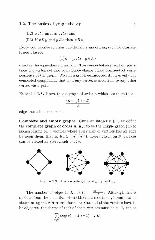
Complete and empty graphs. Given an integer n ≥ 1, we define
the complete graph of order n, Kn, to be the unique graph (up to
isomorphism) on n vertices where every pair of vertices has an edge
between them; that is, Kn ≅ ([n], [n]2). Every graph on N vertices
can be viewed as a subgraph of KN .
1
2
3
4
12
34
5
12
3
4 5
6
Figure 1.5. The complete graphs K4, K5, and K6
The number of edges in Kn is (n2
) = n(n−1)2
. Although this is
obvious from the definition of the binomial coefficient, it can also be
shown using the vertex-sum formula: Since all of the vertices have to
be adjacent, the degree of each of the n vertices must be n−1, and so
∑v∈V
deg(v) = n(n − 1) = 2∣E∣.

10 1. Graph Ramsey theory
1
2
3
4
5
6
7
Figure 1.6. The set {1,2,3,4} forms a 4-clique, whereas theset {5,6,7} is independent.
The complete graph is on one extreme end of a spectrum where
every possible edge is included in the edge set. On the other end,
we would have the graph where none of the vertices are adjacent.
The edge set of this graph is empty, and so we call it the empty
graph. Note that the complete and empty graphs on n vertices are
complements of each other.
Given a graph G = (V,E), if V ′ is a subset of V and G∣V ′ is
complete, then we say that V ′ is a clique. Specifically, if V ′ has
order k, then V ′ is a k-clique.
On the other hand, if G∣V ′ is an empty graph, then we say that
V ′ is independent (see Figure 1.6).
Bipartite and k-partite graphs. Let G = (V,E) be a graph, and
let V be partitioned into V1 and V2; that is, V1∪V2 = V and V1∩V2 = ∅.
Consider the case where E ⊆ V1 × V2 ⊂ [V ]2, so that each edge has
one endpoint in V1 and one endpoint in V2. Such a graph is called a
bipartite graph. An equivalent definition is that the vertex set can
be partitioned into two independent subsets.
Notice that in the right example in Figure 1.7, no more edges
could have been added to that graph without destroying its bipar-
titeness; every vertex in the left column is adjacent to every vertex

1.2. The basics of graph theory 11
1
1
1
1
1
1
1
1
1
1
1
1
1
1
Figure 1.7. Two bipartite graphs
1
1
1 1
1
1
1
11 1
Figure 1.8. A 3-partite graph
in the right column. If G = (V1 ∪ V2,E) is a bipartite graph where
∣V1∣ = n and ∣V2∣ = m, and every vertex in V1 is adjacent to every
vertex in V2, then G is the complete bipartite graph of order
n,m, and we denote it by Kn,m.
Exercise 1.9. Describe the complement of Kn,m.
We can generalize the definition of bipartite to say that a graph
is k-partite if the vertex set can be partitioned into k independent
subsets.
If G is a k-partite graph whose vertex set is partitioned into V1
through Vk, where ∣Vi∣ = ni and each vertex of Vi is adjacent to every
vertex in all the Vj with j ≠ i, then our graph is the complete k-
partite graph of order n1, . . . , nk, and we denote it by Kn1,...,nk.

12 1. Graph Ramsey theory
Exercise 1.10. Prove that the total number of edges in Kn1,...,nkis
∑1≤i<j≤k
ninj .
Trees. A tree is a connected graph which contains no cycles. Trees
show up in many fields of math, but also across many disciplines,
from decision trees to phylogenetic trees.
1
1
1
1
1
1
1
1
1
1
1
1
Figure 1.9. A tree
Theorem 1.11. A graph is a tree if and only if there is a unique
path between any two vertices.
Proof. Assume there are two paths that connect vertices u and v. We
may also assume that the two paths do not share any vertices except
for u and v, since in that case we could replace u or v by the first vertex
that the two paths share (and obtain two shorter paths to which we
could apply the argument). We can create a cycle by concatenating
the paths in the following way: If the first path goes through the
vertices u, x1, . . . , xn, v and the second path goes through the vertices
u, y1, . . . , ym, v, take u, x1, . . . , xn, v, ym, . . . , y1, u. Therefore, a tree
will always have a unique path between any two vertices.
On the other hand, assume that we have a graph G which is not
a tree. This means that either G is disconnected or there is a cycle in
G. If G is disconnected, then there are two vertices u and v that are
in different connected components and so do not have a path between
them. If G has a cycle, the cycle contains at least two vertices, u′ and
v′. This path can then be decomposed into two paths, one from u′

1.2. The basics of graph theory 13
to v′ and one from v′ to u′, which means that there is more than one
path between the two vertices. Therefore, any graph in which there is
a unique path between any two vertices would be a connected graph
with no cycles, a tree. �
Exercise 1.12. Prove that a graph is a tree if and only if removing
an edge makes the graph disconnected.
Exercise 1.13. Prove that a connected graph on n vertices is a tree
if and only if it has n − 1 edges.
The fact that two vertices are connected by a unique path lets us
organize a tree in a hierarchical manner. We designate one vertex in
a tree to be the root of the tree. Then, any other vertex in the tree
with degree 1 is called a leaf. Once a root has been chosen, we can
reorient any tree with the root at the bottom and all the leaves at
the top, like a real tree.
After choosing a root vertex, we can partially order the vertices
of a tree, based on their distance from the root. Given a vertex v,
consider the unique path from the root r to v. If this path goes
through a vertex u, then we say that v is a successor of u, or that u
is a predecessor of v, and we write u < v.
This order is partial in the sense that if u ≠ v are not on the same
path from the root, they are not comparable, that is, neither u < v
nor v < u.
The root is the unique vertex which is a predecessor of all other
vertices. A path from the root r to v can be represented as the
sequence of vertices
r = v0 < v1 < ⋯ < vn−1 < vn = v,
where each vi is an immediate successor of vi−1.
The induced partial order is an important aspect of trees, and we
will return to it in Section 2.2.
Graph colorings. Graph colorings generally come in two varieties:
edge colorings and vertex colorings. Since we are using graphs as a
means of illustrating subsets of [V ]2 as edges, we will be primarily

14 1. Graph Ramsey theory
interested in edge colorings. Given a graph G = (V,E), an r-edge
coloring, or simply r-coloring, of G is a function c ∶ E → [r].Any graph G = (V,E) on N vertices induces a 2-coloring on KN
in the following way: If two vertices are adjacent in G, paint their
edge in KN blue; otherwise paint it red.
12
3
4 5
6
An arbitrary graph of order 6
12
3
4 5
6
The induced coloring of K6
Figure 1.10. Translating between arbitrary graphs and edgecolorings of a complete graph (⋯ = blue, −− = red)
The induced coloring can also be seen as a set partition of [V ]2into two complementary parts E1 and E2; we can color the edges in
E1 blue and those in E2 red, and (V,E1) and (V,E2) will be graph
complements in KN . Likewise, we can view an r-coloring as repre-
senting a set partition of [V ]2 into r parts, resulting in r mutually
exclusive graphs.
1.3. Ramsey’s theorem for graphs
Suppose you arrive at a party. As you browse the room, you see some
familiar faces, whereas others are complete strangers to you. As you
make your way to the buffet, a curious thought enters your mind:
Will there be at least three people who all know each other? And if
not, are there three people who have never met before?
As you are mathematically inclined, you notice your question
has a graph-theoretic formulation: We can represent each guest by a
vertex. If two guests know each other, we draw a blue line between
them, and if they have never met, we draw a red line between them.

1.3. Ramsey’s theorem for graphs 15
What we have is a representation of the party as a 2-coloring of Kn,
where n is the number of guests.
Now the original question becomes:
If we 2-color the edges of Kn, can we find a red or a blue
triangle?
Exercise 1.14. Show that if only five people attend, the answer to
your question can be negative. In other words, find a 2-coloring of
K5 without a monochromatic triangle.
So let us assume there are at least six people attending and con-
sider any 2-coloring of K6. Let us call the vertices v1, v2, . . . , v6 and
consider, without loss of generality, the first vertex v1. Vertex v1 is
connected to five other vertices. If we let R be the set of vertices con-
nected to v1 by a red edge and let B be the set of vertices connected
to v1 by a blue edge, then by the pigeonhole principle, either ∣R∣ ≥ 3
or ∣B∣ ≥ 3; we will assume ∣R∣ ≥ 3. If any two elements in R, say v2 and
v3, are connected by a red edge, then v1, v2, and v3 are the vertices
of a red triangle. On the other hand, if all the elements in R are
connected by blue edges, then we have a blue triangle since there are
at least three vertices in R. In either case, we have a monochromatic
triangle (Figure 1.11).
In arrow notation, we just showed that 6 �→ (3)22. (Keep in
mind that the subscript is denoting that we are using 2 colors, and
the superscript is denoting that we are coloring 2-element subsets.)
Surely this result will hold if our original complete graph was on
more than six vertices; simply pick six of the vertices and consider
the induced subgraph on those vertices, which is necessarily K6, and
then use the result. Since we previously showed that five vertices is
not enough, we have proven the following.
Proposition 1.15. N �→ (3)22 if and only if N ≥ 6.
We should note how important the pigeonhole principle was to
our argument, specifically that 5 �→ (3)12. Note also that while we
end up with a monochromatic subset, we do not know in advance
which color it will have. This only becomes clear during the process
of finding it.

16 1. Graph Ramsey theory
v1v2
v3
v4 v5
v6
We start with a 2-colored K6. Pickan arbitrary vertex, for example v1.
v1v2
v3
v4 v5
v6
Three edges connecting v1 to theother vertices are “red” (dashed).The vertices at the other end of these
edges are v2, v3, and v4.
v1v2
v3
v4 v5
v6
The edges between v2, v3, and v4 areall “blue” (dotted), yielding the de-sired monochromatic K3. Were oneof the edges red, its vertices, togetherwith v1, would give rise to a red
(dashed) triangle.
Figure 1.11. Proving 6 → (3)22
If the party has more guests, can we find even larger cliques (of
mutual friends or mutual strangers)? This is the subject of Ramsey’s
theorem for graphs.
Theorem 1.16 (Ramsey’s theorem for 2-colored graphs). For any
k ≥ 2, there exists some integer N such that any 2-coloring of a graph

1.3. Ramsey’s theorem for graphs 17
of at least N vertices contains a complete monochromatic subgraph
on k vertices.
Proposition 1.15 was a special case of this statement. There, we
saw that for k = 3 we can choose N = 6. The dual form of the theorem,
using cliques and independent sets, reads as follows.
Corollary 1.17 (Ramsey’s theorem for graphs, dual form). For any
k ≥ 2, there exists some integer N such that any graph of at least N
vertices contains a complete subgraph on k vertices or an independent
subgraph on k vertices.
In the course of this book, we will encounter several proofs of
Theorem 1.16. We start with the one that is not the most elegant
but arguably the most elementary, as it uses the pigeonhole principle
in an almost “brute force” way.
Proof of Theorem 1.16. Consider KN , the complete graph on N
vertices, where we think of N for now as a sufficiently large integer.
Suppose the edges of KN are 2-colored, red and blue.
We will construct a monochromatic Kk in two stages. In the first
stage, we pick a sequence of vertices
v1, v2, v3, . . .
such that vi is connected to all following vertices by an edge of the
same color. This color, however, may change from vertex to vertex.
In the second stage, we select a subsequence from the vi that yields
a monochromatic Kk.
Stage 1: We start by picking an arbitrary vertex v1 and consider
theN−1 remaining vertices. These are split into two subsets: the ones
we call the blue vertices because they connect to v1 via a blue edge,
and the red vertices that connect via a red edge. By the pigeonhole
principle, there are either ⌈(N −1)/2⌉ red or ⌈(N −1)/2⌉ blue vertices.Call the color for which this holds c1 and let V2 be the set of color-c1vertices, that is, vertices that connect to v1 via an edge of color c1.
V2 induces a subgraph G2 = (V2,E2) (E2 contains all edges between
vertices in V2).

18 1. Graph Ramsey theory
We now continue working in G2 and repeat the whole process
by choosing an arbitrary vertex v2 ∈ V2. G2 has at least ⌈(N − 1)/2⌉vertices, so again by the pigeonhole principle, there are at least
⌈⌈N−1
2⌉ − 1
2⌉ ≥ ⌈N − 3
4⌉
vertices in G2 that are connected to v2 by an edge of the same color.
Call this color c2. We collect the vertices adjacent to v2 via these
edges in the set V3, which in turn induces a new subgraph G3 of G2.
If we continue this process, we get a sequence of vertices
v1, v2, v3, . . . , vt
and a sequence of colors
c1, c2, c3, . . . , ct
(and a sequence subgraphs G = G1 ⊃ G2 ⊃ G3 ⊃ ⋅ ⋅ ⋅ ⊃ Gt). Since we
“take out” at least one vertex in each step, the process will terminate
after finitely many, say t, steps, because the graph we started with
has only finitely many vertices. By the way we chose these sequences,
they have the following property:
For any vertex vi in the sequence, all later vertices vj with
j > i are connected to vi by an edge of color ci.
We are not quite done yet, because the colors ci can be different for
each vertex. If these colors were all identical, the whole sequence
v1, v2, . . . would induce a complete monochromatic subgraph.
Stage 2: We use the pigeonhole principle one more time. Among
the color sequence c1, c2, c3, . . . , ct, one color must occur at least half
the time. Let c be such a color. Now consider all the vertices vifor which ci = c. Collect them in a vertex set Vc. We claim that Vc
induces a complete monochromatic subgraph of color c. Let v and
w be two vertices in Vc. They have entered the sequence at different
stages, say v = vi0 and w = vi1 , where i0 > i1. But, by definition of Vc,
every edge between vi0 and a later vertex is of color ci0 = c. Since v
and w were arbitrary vertices of Vc, all edges between vertices in Vc
have color c.

1.3. Ramsey’s theorem for graphs 19
v1 connects via a blue edge
v1 connects via a red edge
v2 connects via a blue edgev1
v2
Figure 1.12. Selecting the sequence of nodes v1, v2, . . .
We have hence a set of vertices Vc of cardinality ≥ ⌈t/2⌉ that
induces a monochromatic subgraph. We want a complete graph with
k vertices. That means we need to choose N large enough so that
⌈t/2⌉ ≥ k.
A straightforward induction yields that for s < t,
∣Gs+1∣ ≥ ⌈N − (2s − 1)2s
⌉ ≥ N
2s− 1.
This means that Stage 1 has at least ⌊log2N⌋ have steps, i.e. t ≥⌊log2N⌋. This in turns implies that if we let
N = 22k,

20 1. Graph Ramsey theory
we get a monochromatic complete subgraph of size
log2 22k
2= k.
�Exercise 1.18. Use Ramsey’s theorem for graphs to show that for
every positive integer k there exists a number N(k) such that if
a1, a2, . . . , aN(k) is a sequence ofN(k) integers, it has a non-increasing
subsequence of length k or a non-decreasing subsequence of length k.
Show further that N(k + 1) > k2.
(Hint: Find a way to translate information about sequences rising orfalling into a graph coloring.)
Multiple colors. In our treatment so far we have dealt with 2-
colorings of complete graphs, mainly because of the nice correspon-
dence between monochromatic complete subgraphs and cliques/inde-
pendent sets as described in Figure 1.10. But Theorem 1.16 can be
extended to hold for any finite number of colors.
Theorem 1.19. For any k ≥ 2 and for any r ≥ 2 there exists some
integer N such that any r-coloring of a complete graph of at least N
vertices contains a complete monochromatic subgraph on k vertices.
The proof of this theorem is very similar to the proof of Theo-
rem 1.16. One can in fact go through it line by line and adapt it to
the case of r colors; we will simply give the broad strokes.
In Stage 1, we choose a vertex v0 and partition the other vertices
by the color of the edge they share with v0. The largest of the subsets
will have size at least 1/r times the first set. If we started with N
vertices, this process will terminate in t steps where t ≥ ⌊logr N⌋. So
if we choose N = rrk, then our process will terminate in rk steps or
more.
Now, in Stage 2, we have a sequence of rk vertices, each connected
to all of the following vertices by the same color. This color, however,
can differ from vertex to vertex, one of r many colors. Another ap-
plication of the pigeonhole principle as in the proof of Theorem 1.16
gives us a set of k vertices that all connect to all subsequent vertices
by a single color. These vertices form a monochromatic k-clique.
Therefore, rrk �→ (k)2r.

1.4. Ramsey numbers and probabilistic method 21
Exercise 1.20. Prove Schur’s theorem: For every positive integer k
there exists a number M(k) such that if the set {1, 2, . . . ,M(k)} is
partitioned into k subsets, at least one of them contains a set of the
form {x, y, x + y}.
(Hint: Consider a complete graph on vertices {0, 1, 2, . . . ,M}, where
M is an integer. Devise a k-coloring of the graph such that the color of
an edge reflects an arithmetic relation between the vertices with respect to
the k-many partition sets.)
1.4. Ramsey numbers and the probabilisticmethod
As we described in the introduction, Ramsey’s theorem is remarkable
in the sense that it guarantees regular substructures in any sufficiently
large graph, no matter how “randomly” that graph is chosen. But how
large is “sufficiently large”?
Definition 1.21. The Ramsey number R(k) is the least natural
number N such that N �→ (k)22.
From our proof of Ramsey’s theorem (Theorem 1.16) we obtain an
upper bound R(k) ≤ 22k. Is this bound sharp? It gives us R(3) ≤ 64,
while we already saw in the previous section that R(3) = 6 (Proposi-
tion 1.15). The proof yields R(10) ≤ 220 = 1 048 576, but it was shown
in 2003 [59] that R(10) ≤ 23 556; in fact the true value of R(10) could
still be much lower. It seems that we have just been a little “wasteful”
when proving Ramsey’s theorem for graphs, using way more vertices
in our argument than actually required. This leads us to the ques-
tion of finding better upper and lower bounds for Ramsey numbers, a
notoriously difficult problem.
In 1955, Greenwood and Gleason published a paper [27] which
provided the first exact Ramsey numbers for k > 3, as well as answers
to generalizations of the problem. Their proof is a nice example of
the fact that sometimes it is easier to prove a more general statement.
Instead of finding monochromatic cliques of the same order, one
can break the symmetry and look for cliques of different orders—for
example, either a red m-clique or a blue n-clique. We can extend our

22 1. Graph Ramsey theory
arrow notation by saying that
N �→ (m,n)22if every 2-coloring of a complete graph of order N has either a red
complete subgraph on m vertices or a blue complete subgraph on n
vertices.
Definition 1.22. The generalized Ramsey number R(m,n) is
the least integer N such that N �→ (n,m)22.
The Ramsey number R(k) introduced at the beginning of this
section is equal to the diagonal generalized Ramsey number R(k, k).It is clear that R(m,n) exists for every pair m,n, since R(m,n) ≤
R(k) when k = max(m,n). On the other hand, R(m,n) ≥ R(k) when
k = min(m,n). Since one can swap the colors on all the edges from
red to blue or from blue to red, R(m,n) = R(n,m).Some values of R(m,n) are known. We put R(m, 1) = R(1, n) = 1
for all m,n, since K1 has no edges. Any single vertex is, trivially, a
monochromatic 1-clique of any color.5 If we consider finding R(m, 2),we are looking for either a red m-clique or a blue 2-clique. But if any
edge in a coloring is blue, its endpoint vertices form a monochromatic
2-clique. If a graph does not have a blue edge, it must be completely
red. Therefore R(m, 2) = m, and similarly R(2, n) = n.
Greenwood and Gleason proved a recursive relation between the
Ramsey numbers R(m,n). As their result does not assume the exis-
tence of any diagonal Ramsey number R(k), we in particular obtain
a new, elegant proof of Theorem 1.16.
Theorem 1.23 (Greenwood and Gleason). The Ramsey numbers
R(m,n) exist for all m,n ≥ 1 and satisfy
(1.1) R(m,n) ≤ R(m − 1, n) + R(m,n − 1)for all m,n ≥ 2.
Proof. Wewill proceed by simultaneous induction onm and n, mean-
ing that we deduce that R(m,n) exists using the fact that both
R(m,n−1) and R(m−1, n) exist. To be more specific, we can arrange
5We use this definition only to aid us in induction in the following proofs. Wewill generally ignore this case in discussion.

1.4. Ramsey numbers and probabilistic method 23
the pairs m,n in a matrix and then use the truth of the statement for
values in the ith diagonal of the matrix to prove the statement in the
(i + 1)st diagonal. In each diagonal, the sum m + n is constant, and
so we can view the simultaneous induction on m and n as a standard
induction on the value m + n.
For the base case of the induction (m = n = 2), (1.1) follows easily
from the fact that R(2, n) = n and R(m, 2) = m. For the inductive
step, let N = R(m−1, n) +R(m,n−1). Consider a 2-colored KN and
let v be an arbitrary vertex. Define Vred and Vblue to be the vertices
connected to v via a red edge or a blue edge, respectively. Then
(1.2) ∣Vred∣ + ∣Vblue∣ = N − 1 = R(m − 1, n) + R(m,n − 1) − 1.
By the pigeonhole principle, either ∣Vred∣ ≥ R(m − 1, n) or ∣Vblue∣ ≥R(m,n−1). For if ∣Vred∣ ≤ R(m−1, n) −1 and ∣Vblue∣ ≤ R(m,n−1) −1,
then
∣Vred∣ + ∣Vblue∣ ≤ R(m − 1, n) + R(m,n − 1) − 2.
We want to argue that in either case, KN has either a complete
red subgraph on m vertices or a complete blue subgraph on n vertices.
Let us first assume ∣Vred∣ ≥ R(m − 1, n). From the definition of the
Ramsey number, Vred has either a complete red subgraph on m − 1
vertices or a complete blue subgraph on n vertices. In the second case
we are done right away. In the first case, we can add our chosen v
to the set Vred and the new red subgraph is complete on m vertices.
The argument for ∣Vblue∣ ≥ R(m,n − 1) is similar. �
There is a certain similarity between the inequality in (1.1) and
the famous relationship between binomial coefficients:
(nm
) = (n − 1
m) + (n − 1
m − 1).
We can exploit this recursive relation to arrive at an upper bound for
R(k) which is better than the one we had before.
Theorem 1.24. For all m,n ≥ 2, the Ramsey number R(m,n) sat-
isfies
R(m,n) ≤ (m + n − 2
m − 1).
24 1. Graph Ramsey theory
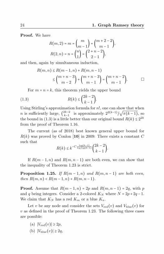
Proof. We have
R(m, 2) = m = ( m
m − 1) = (m + 2 − 2
m − 1),
R(2, n) = n = (n1
) = (2 + n − 2
2 − 1),
and then, again by simultaneous induction,
R(m,n) ≤ R(m − 1, n) + R(m,n − 1)
≤ (m + n − 3
m − 2) + (m + n − 3
m − 1) = (m + n − 2
m − 1). �
For m = n = k, this theorem yields the upper bound
(1.3) R(k) ≤ (2k − 2
k − 1).
Using Stirling’s approximation formula for n!, one can show that when
n is sufficiently large, (2k−2k−1 ) is approximately 22(k−1)/
√π(k − 1), so
the bound in (1.3) is a little better than our original bound R(k) ≤ 22k
from the proof of Theorem 1.16.
The current (as of 2018) best known general upper bound for
R(k) was proved by Conlon [10] in 2009: There exists a constant C
such that
R(k) ≤ k−Clog(k−1)
log log(k−1) (2k − 2
k − 1).
If R(m − 1, n) and R(m,n − 1) are both even, we can show that
the inequality of Theorem 1.23 is strict.
Proposition 1.25. If R(m − 1, n) and R(m,n − 1) are both even,
then R(m,n) < R(m − 1, n) + R(m,n − 1).
Proof. Assume that R(m − 1, n) = 2p and R(m,n − 1) = 2q, with p
and q being integers. Consider a 2-colored KN where N = 2p+ 2q − 1.
We claim that KN has a red Km or a blue Kn.
Let v be any node and consider the sets Vred(v) and Vblue(v) for
v as defined in the proof of Theorem 1.23. The following three cases
are possible:
(a) ∣Vred(v)∣ ≥ 2p,
(b) ∣Vblue(v)∣ ≥ 2q,

1.4. Ramsey numbers and probabilistic method 25
(c) ∣Vred(v)∣ = 2p − 1 and ∣Vblue(v)∣ = 2q − 1.
In cases (a) and (b), we can argue as in the proof of Theorem 1.23
that a monochromatic Km or Kn exists. Case (c) requires a counting
argument, where we will use the parity assumption.
As v was arbitrary, we can carry out the above argument for
all nodes. If for any node (a) or (b) holds, we are done. So let us
assume that for every node v, (c) holds. Every edge has two ends.
We identify the color of the ends with the color of the edge. Since
(c) holds for every node, (2p + 2q − 1)(2p − 1) of the edges have red
ends. (2p + 2q − 1)(2p − 1) is an odd number, but every edge has
two ends, which implies an even number of red ends, leading to a
contradiction. �
Some exact values. For some small values of m,n, we are able
to determine R(m,n) exactly. We have already mentioned that for
m,n ≥ 2, R(m, 2) = m and R(2, n) = n. We have also proved in
Section 1.3 that R(3, 3) = 6.
Proposition 1.26. R(3, 4) = 9 and R(3, 5) = 14
Proof. From Theorem 1.23, we have that R(3,4) ≤ R(3, 3)+R(2, 4) =6 + 4 = 10, and by Proposition 1.25, the inequality is strict. So
R(3, 4) ≤ 9.
Greenwood and Gleason were able to describe a graph of order
13 which has neither a red 3-clique nor a blue 5-clique, implying
that R(3, 5) > 13. Then 14 ≤ R(3, 5) ≤ R(2, 5) + R(3, 4), and since
R(2, 5) = 5, we have R(3, 4) ≥ 9, which proves R(3, 4) = 9; plugging
that back into the inequality gives us R(3, 5) = 14. �
Proposition 1.27. R(4, 4) = 18.
Proof. From Theorem 1.23 and the previous proposition, we have
that R(4, 4) ≤ R(3, 4) + R(4, 3) = 18.
To prove that 18 is the actual value of R(4, 4), we have to producea 2-coloring of a K17 that does not have a monochromatic K4; in fact,
there is exactly one such coloring, which is defined using ideas from
elementary number theory.

26 1. Graph Ramsey theory
Let p be any prime which is congruent to 1 modulo 4. An integer
x is a quadratic residue modulo p if there exists an integer z such
that z2 ≡ xmod p. We can define the Paley graph of order p as
the graph on [p] where the vertices x, y ∈ {1, 2, . . . , p} have an edge
between them if and only if x−y is a quadratic residue modulo p. This
definition does not depend on whether we consider x−y or y−x, since
p ≡ 1 mod 4 and −1 is a square for such prime p. The set of quadratic
residues is always equal in size to the set of quadratic non-residues,
both sets having p−12
elements, as 0 is considered neither a residue
nor a non-residue. The symmetry between quadratic residues and
non-residues also causes the Paley graphs to be self-complementary,
that is, the complement of a Paley graph is isomorphic to itself. At
the root of all this lies the law of quadratic reciprocity, first proved by
Gauss in his Disquisitiones Arithmeticae [18].6
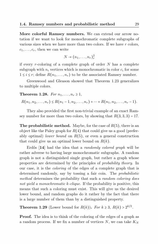
Figure 1.13 shows the Paley graph of order 17; we can use this
graph to induce a 2-coloring on K17. It can be shown using a bit of
elementary number theory that this graph does not have a 4-clique.
Since the graph is also self-complementary, it has no independent sets
of 4 vertices either. Therefore, R(4) = 18. �
Despite their rather regular appearance, the Paley graphs are im-
portant objects in the study of random graphs, as they share many
statistical properties with graphs for which the edge relation is deter-
mined by a random coin toss.
Moving on to higher Ramsey numbers, can we get an exact value
for R(5)? As both R(3, 5) and R(4, 4) are even, Proposition 1.25
gives us
R(4, 5) ≤ R(3, 5) + R(4, 4) − 1 = 31,
and hence
R(5, 5) ≤ R(4, 5) + R(5, 4) ≤ 62.
However, in this case the upper bound for R(4, 5) turned out
not to be exact. In 1995, McKay and Radziszowski [45] showed that
R(4, 5) = 25. This in turn improved the upper bound for R(5, 5) to
R(5, 5) ≤ 49.
6For a proof of the reciprocity law as well as for further background in numbertheory, the book by Hardy and Wright [31] is a classic yet hardly surpassed text.

1.4. Ramsey numbers and probabilistic method 27
1
2
3
45 6
7
8
9
10
11
12
131415
16
17
Figure 1.13. The Paley graph of order 17. The quadraticresidues modulo 17 are 1, 2, 4, 8, 9, 13, 15, and 16. Thisgraph does not contain K4 as a subgraph.
At this point, one may ask: There are only finitely many 2-
colorings of a complete graph of any finite order. Could we not cycle
through all colorings of K48 one by one (preferably on a fast com-
puter) and check whether each has either a red or a blue 5-clique? If
not, then R(5) = 49. If yes, then we could test all 2-colorings of a
K47, and so on. Eventually we will have determined the fifth Ramsey
number.
The problem with this strategy is that there are simply too many
graphs to check! How many colorings are there? A K48 has (482
) =1128 edges. Each edge can be colored in two ways, giving us
21128 ≈ 3.6 × 10339
colorings to check. At the time this book was written, the world’s
fastest supercomputer, the Cray Titan, could perform about 20×1015
floating-point operations per second (FLOPS). Under the unrealistic
28 1. Graph Ramsey theory
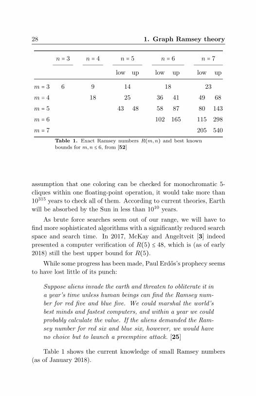
n = 3 n = 4 n = 5 n = 6 n = 7
low up low up low up
m = 3 6 9 14 18 23
m = 4 18 25 36 41 49 68
m = 5 43 48 58 87 80 143
m = 6 102 165 115 298
m = 7 205 540
Table 1. Exact Ramsey numbers R(m,n) and best knownbounds for m,n ≤ 6, from [52]
assumption that one coloring can be checked for monochromatic 5-
cliques within one floating-point operation, it would take more than
10315 years to check all of them. According to current theories, Earth
will be absorbed by the Sun in less than 1010 years.
As brute force searches seem out of our range, we will have to
find more sophisticated algorithms with a significantly reduced search
space and search time. In 2017, McKay and Angeltveit [3] indeed
presented a computer verification of R(5) ≤ 48, which is (as of early
2018) still the best upper bound for R(5).While some progress has been made, Paul Erdos’s prophecy seems
to have lost little of its punch:
Suppose aliens invade the earth and threaten to obliterate it in
a year’s time unless human beings can find the Ramsey num-
ber for red five and blue five. We could marshal the world’s
best minds and fastest computers, and within a year we could
probably calculate the value. If the aliens demanded the Ram-
sey number for red six and blue six, however, we would have
no choice but to launch a preemptive attack. [25]
Table 1 shows the current knowledge of small Ramsey numbers
(as of January 2018).
1.4. Ramsey numbers and probabilistic method 29
More colorful Ramsey numbers. We can extend our arrow no-
tation if we want to look for monochromatic complete subgraphs of
various sizes when we have more than two colors. If we have r colors,
c1, . . . , cr, then we can write
N → (n1, . . . , nr)2rif every r-coloring of a complete graph of order N has a complete
subgraph with ni vertices which is monochromatic in color ci for some
1 ≤ i ≤ r; define R(n1, . . . , nr) to be the associated Ramsey number.
Greenwood and Gleason showed that Theorem 1.23 generalizes
to multiple colors.
Theorem 1.28. For n1, . . . , nr ≥ 1,
R(n1, n2, . . . , nr) ≤ R(n1 − 1, n2, . . . , nr) + ⋯ + R(n1, n2, . . . , nr − 1).
They also provided the first non-trivial example of an exact Ram-
sey number for more than two colors, by showing that R(3, 3, 3) = 17.
The probabilistic method. Maybe, for the case ofR(5), there is anobject like the Paley graph for R(4) that could give us a good (prefer-
ably optimal) lower bound on R(5), or even a general construction
that could give us an optimal lower bound on R(k).Erdos [14] had the idea that a randomly colored graph will be
rather adverse to having large monochromatic subgraphs. A random
graph is not a distinguished single graph, but rather a graph whose
properties are determined by the principles of probability theory. In
our case, it is the coloring of the edges of a complete graph that is
determined randomly, say by tossing a fair coin. The probabilistic
method determines the probability that such a random coloring does
not yield a monochromatic k-clique. If the probability is positive, this
means that such a coloring must exist. This will give us the desired
lower bound, and random graphs do it rather by the fact that there
is a large number of them than by a distinguished property.
Theorem 1.29 (Lower bound for R(k)). For k ≥ 3, R(k) > 2k/2.
Proof. The idea is to think of the coloring of the edges of a graph as
a random process. If we fix a number of vertices N , we can take KN

30 1. Graph Ramsey theory
and color each of the (N2
) edges based on a fair coin flip, say red for
heads and blue for tails. Since the coin flips are independent, there
will be a total of 2(N2) different 2-colorings of KN , each occurring with
equal probability.
Pick k vertices in your graph. There are 2(k2) possible 2-colorings
of this subgraph and exactly 2 of them are monochromatic. Therefore,
the probability of randomly getting a monochromatic subgraph on
these k vertices is 21−(k2). There are (N
k) different k-cliques in KN ,
so the probability of getting a monochromatic subgraph on any k
vertices is (Nk
)21−(k2).Now suppose N = 2k/2. We want to show that there is a positive
probability that a random coloring ofKN will have no monochromatic
k-clique (and hence deduce that R(k) > 2k/2, proving the theorem).
We bound the probability that a random coloring will give us a
monochromatic k-clique from above:
(Nk
)21−(k2) = N !
k!(N − k!)21−(k2)
≤ Nk
k!21−(
k2) (since N !
(N − k)! ≤ Nk)
= 2k2/2
k!21−(k
2−k)/2
= 21+k/2
k!.
If k ≥ 3, then 21+k/2
k!< 1. (This is easily verified by induction.) There-
fore, it is not certain to always obtain a monochromatic clique of size
k, which in turn means that there is a positive probability that a
random coloring of KN will have no monochromatic k-clique. �
While Erdos was not the first to use this kind of argument, he
certainly popularized it and, through his results, helped it become an
important tool not only in graph theory and combinatorics but also
in many other areas of mathematics (see for example [2]).

1.5. Turan’s theorem 31
1.5. Turan’s theorem
While Ramsey’s theorem tells us that in a 2-coloring of a sufficiently
large complete graph we always find a monochromatic clique, we do
not know what color that clique will be. One would think that if there
were quite a few more red edges than blue edges, we would be assured
a red clique—but how many “more” red than blue do we need?
As before, rather than talking about 2-colorings of a complete
graph, we can rephrase this discussion in terms of the existence of
cliques. We should expect that a graph with a lot of edges should
contain a complete subgraph, but what do we mean by “a lot”? This
is the subject of Turan’s theorem [65].
Theorem 1.30 (Turan’s theorem). Let G = (V,E), where ∣V ∣ = N ,
and let k ≥ 2. If
∣E∣ > (1 − 1
k − 1) N2
2,
then G has a k-clique.
In graph theory texts, this often phrased as a result about k-
clique-free graphs: If a graph has no k-clique, then it has at most
(1 − 1k−1) N2
2edges. In his proof, Turan provided examples of graphs,
now called Turan graphs, which have exactly (1 − 1k−1) N2
2edges and
no k-cliques. Turan graphs are the largest graphs such that adding
any edge would create a k-clique, and are therefore considered to
be extremal. Extremal graphs, the largest (or smallest) graphs with
a certain property, are the objects of interest in the field of extremal
graph theory, for which Turan’s theorem is one of the founding results.
If we begin with k = 3, our goal is to find a graph on N vertices
with as many edges as possible but with no triangles. For this, we
have to look no further than bipartite graphs. Indeed, if {v1, v2} and
{v2, v3} are in the edge set of some bipartite graph, then v1 and v3are elements of the same part, and are therefore not connected. This
is true for any bipartite graph, but the complete bipartite graphs will
have the most edges.
For N = 6, we can look at the bipartite graphs K1,5, K2,4, and
K3,3 and note that these graphs have 5, 8, and 9 edges respectively.

32 1. Graph Ramsey theory
Objects in mathematics tend to achieve maxima when the sizes of
parts involved are balanced. The rectangle with the largest area-to-
perimeter ratio is the one where the sides have equal length. Likewise,
our graph Kn,m will have a maximal number of edges when the sizes
n and m are balanced.
We can extend this example to k > 3 by considering complete
(k − 1)-partite graphs. It is clear by the pigeonhole principle that
these graphs have no k-clique; any complete subgraph can choose
only one vertex from each of the (k − 1) subsets of vertices. Proving
Turan’s theorem would just require us to optimize this process for a
maximal number of edges.
As before, our graph Kn1,...,nk−1will have a maximal number of
edges when the ni are balanced so that the subsets all have the same
number of vertices, or at worst are within 1 of each other when the
total number of vertices is not evenly divisible by k − 1. For if our
subset sizes were unbalanced, that is, if ni − nj ≥ 2 for some Vi and
Vj , we can switch a vertex from Vi to Vj . Then the number of edges
between Vi and Vj changes from ninj to
(ni − 1)(nj + 1) = ninj + ni − nj − 1 > ninj .
We also have that the number of edges between Vi and Vj with any
other set does not change. So, heuristically, the optimal graphs for
this approach are Kn1,...,nk−1where ∣ni − nj ∣ ≤ 1 for all i, j; these are
called Turan graphs.
In particular, if we can equally distribute the N vertices (that
is, N is divisible by k − 1), we get the Turan graph K(n,...,n) where
n = Nk−1 . The number of edges in this graph is
(k − 1
2)n2 = (k − 1)(k − 2)
2
N2
(k − 1)2 = (1 − 1
k − 1) N2
2.
This value is known as the (k−1)st Turan number, tk−1(N). In 1941,
Pal Turan proved that these graphs do in fact provide the best bound
possible. Next, we give a formal proof of this result.
Proof of Turan’s theorem. Let G = (V,E) be a graph on N ver-
tices which does not have a k-clique. We are going to transform G
into a graph H which has at least as many edges as G and still does

1.5. Turan’s theorem 33
vmax
S T
Figure 1.14. Constructing the graph H: The edges betweennodes in S remain (dotted); the edges between nodes in T areremoved; every vertex in S is connected to every vertex in T(dashed).
not have a k-clique in the following manner: Choose a vertex vmax
of maximal degree. We can now partition our vertex set into two
subsets; let S be the subset of vertices in G adjacent to vmax and
let T ∶= V ∖ S. To go from G to H, first remove any edges between
vertices in T . Then, for every vertex v ∈ T and vertex v′ ∈ S, connect
v to v′ (if they are not already connected). See Figure 1.14. Note
that vmax ∈ T .We will now demonstrate that the number of edges in H is no
smaller than the number of edges in G. To do so, we will utilize the
fact that
∣E∣ = 1
2∑v∈V
d(v),
where d(v) is the degree of the vertex v. It is enough to show that
dH(v) ≥ dG(v) for every v ∈ V , i.e. every vertex has degree at least as
high in H as in G.
If v ∈ T , then, by our construction, dH(v) = dG(vmax) ≥ dG(v)since vm had maximal degree.
If v ∈ S, we know the degree of v in H can only increase since it
is adjacent to the same vertices in S and now also adjacent to every
vertex in T .

34 1. Graph Ramsey theory
We claim that H has no k-clique. Clearly, any clique can have at
most one vertex in T and so it suffices to show that S does not have
a (k − 1)-clique. However, this is true since G has no k-cliques: If we
had a (k − 1)-clique in S, we could add the vertex vmax, which would
be adjacent to every vertex in the clique, thus forming a k-clique in
G.
We can now apply the same transformation to the subgraph in-
duced by S, and inductively to the corresponding version of S in that
graph. In this way, we eventually end up with a (k−1)-partite graph.(Note that, by construction, none of the vertices in T share an edge
in H.) And our construction also shows that if G is a graph on N
vertices with no k-clique, there is also a (k − 1)-partite graph on N
vertices that has at least as many edges as G. But we already know
that among the (k − 1)-partite graphs, the Turan graphs have the
maximal number of edges. �
1.6. The finite Ramsey theorem
Two-element subsets of a set S can be represented as graphs, and
this provided a visual framework for much of this chapter. Ramsey’s
theorem, however, holds not only for pairs, but in general for arbitrary
p-element subsets.
Theorem 1.31 (Ramsey’s theorem in its general form). For any
r, k ≥ 2 and p ≥ 1, there exists some integer N such that
N �→ (k)pr .
One can represent p-element subsets as hypergraphs. In a hyper-
graph, any (non-zero) number of vertices can be joined by an edge,
instead of just two (as in graphs). In other words, for a hypergraph,
the edge set is a subset of P(V ) ∖ {∅}, where P(V ) is the power set
of V . If the number of vertices in an edge is constant throughout the
hypergraph, we speak of a uniform hypergraph. The hypergraphs of
interest in the general Ramsey theorem are therefore p-uniform hyper-
graphs. For example, in Figure 1.15 we see 3-uniform hypergraphs.
Recall that when we first proved Ramsey’s theorem for graphs
(the p = 2 case of the theorem above), we relied heavily on the pi-
geonhole principle (the p = 1 case). This suggests that we might want
1.6. The finite Ramsey theorem 35
to try to use induction on p. With this in mind, let’s see how we can
prove the p = 3 case from what we already know, and then show how
to proceed with the induction. We will also focus on the case of two
colors (r = 2) for now and then discuss what needs to be changed to
adapt our argument for more than two colors.
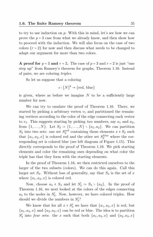
A proof for p = 3 and r = 2. The case of p = 3 and r = 2 is just “one
step up” from Ramsey’s theorem for graphs, Theorem 1.16. Instead
of pairs, we are coloring triples.
So let us suppose that a coloring
c ∶ [N]3 → {red, blue}
is given, where as before we imagine N to be a sufficiently large
number for now.
We can try to emulate the proof of Theorem 1.16. There, we
started by picking a arbitrary vertex v1 and partitioned the remain-
ing vertices according to the color of the edge connecting each vertex
to v1. This suggests starting by picking two numbers, say a1 and a2,
from {1, . . . ,N}. Let S2 ∶= {1, . . . ,N} ∖ {a1, a2}. We can partition
S2 into two sets: one set Sred2 containing those elements x ∈ S2 such
that {a1, a2, x} is colored red and the other set Sblue2 where the cor-
responding set is colored blue (see left diagram of Figure 1.15). This
directly corresponds to the proof of Theorem 1.16. We pick starting
elements and color the remaining ones depending on what color the
triple has that they form with the starting elements.
In the proof of Theorem 1.16, we then restricted ourselves to the
larger of the two subsets (colors). We can do this again. Call this
larger set S3. Without loss of generality, say that S3 is the set of x
where {a1, a2, x} is colored red.
Now, choose a3 ∈ S3 and let S′3 ∶= S3 ∖ {a3}. In the proof of
Theorem 1.16, we next looked at the colors of the edges connecting
a3 to the nodes in S′3. Now, however, we have colored triples. How
should we divide the numbers in S′3?
We know that for all x ∈ S′3 we have that {a1, a2, x} is red, but
{a1, a3, x} and {a2, a3, x} can be red or blue. The idea is to partition
S′3 into four sets: the x such that both {a1, a3, x} and {a2, a3, x}

36 1. Graph Ramsey theory
a1
a2
Coloring the remaining numbers
a1
a2
a3
x
The color configuration of x is
(red, blue).
Figure 1.15. The proof of Ramsey’s theorem for triples
are red, the x such that both triples are blue, the x where the first
triple is red and the second is blue, and the x where the first triple
is blue and the second is red. Each set represents how x is colored
with respect to the numbers already selected. Think of these sets as
“coloring configurations” (see right diagram of Figure 1.15).
One of these four sets must be the largest (or, at least, not smaller
than any of the other three); call this largest set S4. Note that if i
and j are distinct elements from {1, 2, 3}, then c(ai, aj , x) is constant
for all x ∈ S4 and therefore depends not on our choice of x but only
on ai and aj .
We can then continue inductively to find a sequence of elements
a1, a2, . . . , at: At the beginning of stage t, we have already defined
a set St−1 = {a1, a2, . . . , at−1}. We first pick an arbitrary element atin St−1 and put S′t−1 = St−1 ∖ {at}. Next, we determine the color
configurations of all x ∈ S′t−1. This involves checking the color of all
triples {ai, at, x} where i < t. Each color configuration can be thought
of as a sequence of length t−1 recording the colors of the {ai, at, x}, for

1.6. The finite Ramsey theorem 37
example (red, blue, red, red, . . . ). We see that there are 2t−1 possible
color configurations for x. Now partition S′t−1 into 2t−1 sets, where x
and y are in the same set if they have the same color configuration.
From these 2t−1 sets, pick one of maximal size and make this set St.
As before, we have that if 1 ≤ i < j ≤ t, then c(ai, aj , x) is constant
for all x ∈ St. The color depends only on our choice of i and j.
We can carry out this construction till we run out of numbers,
that is, till St consists of one number only; call this number at+1.
We have constructed a sequence a1, a2, . . . , at+1. This sequence
does not yet define a monochromatic subset, but by the way we con-
structed it we can trim it down to one. The crucial property this
sequence inherits from our construction is the following:
(1.4)Whenever we pick 1 ≤ i < j < s ≤ t + 1,
c(ai, aj , as) depends only on i and j, not on s.
The reason is simple: as is eventually chosen from Ss−1, which
is a subset of Sj , and for all numbers x ∈ Sj , we know they have
the same color configuration when forming triples with numbers from
{a1, . . . , aj}. In particular, {ai, aj , x} has the same color for all x ∈Sj+1.
In the proof of Theorem 1.16, we used the pigeonhole principle
in Stage 2 to trim the sequence of an down to a monochromatic one.
Now we use Ramsey’s theorem for graphs (i.e. this theorem for p = 2)
to do so.
We define a new coloring of pairs from the sequence (a1, . . . , at):
c∗ ∶ [N]2 → {red, blue}c∗(ai, aj) ∶= c(ai, aj , as),
where i < j < s ≤ t + 1. This coloring is well-defined by virtue of
(1.4). Now, by Ramsey’s theorem for graphs, if t is large enough
so that t �→ (k)22, we have a monochromatic subset {b1, . . . , bk} ⊆{a1, . . . , at} for c∗. By our definition of c∗, this implies the existence
of a monochromatic subset for c, because for any {bj1 , bj2 , bj3} with
j1 < j2 < j3 we know that
c(bj1 , bj2 , bj3) = c∗(bj1 , bj2)
is constant.
38 1. Graph Ramsey theory
To complete the proof, we have to argue that t can indeed be
obtained large enough so t → (k)22. This is just a matter of picking
the right starting size N . At each stage s of the construction of
the ai, we restrict ourselves to the largest set of remaining numbers
with equal color configurations. As we argued above, there are 2s−1
possible color configurations, so if we have Ns−1 numbers left entering
stage s, we have at leastNs−1 − 1
2s−1
numbers left over after the completion of stage s. If we choose N
large enough, then the sequence
N,N − 2
2,
N−22
− 1
4,
N−22−1
4− 1
8, . . .
reaches 1 after more than R(k) many steps, where R(k) = R(k, k) is
the kth diagonal Ramsey number (see Definition 1.21). Therefore if
N is chosen so that
N ≥ 2(2R(k))2
,
a crude estimate, we obtain a monochromatic subset of size k.
From triples to p-tuples. It should now be clear how to lift this
proof from p = 3 to arbitrary p, using induction. We construct a
sequence of numbers a1, a2, a3, . . . , at+1 such that
(∗p) whenever we pick 1 ≤ i1 < i2 < ⋅ ⋅ ⋅ < ip−1 < s ≤ t + 1, the color
of {ai1 , ai2 , . . . , aip−1 , as} depends only on i1, i2, . . . , ip−1, not
on s.
The construction of such a sequence proceeds similarly to the case
of p = 3, except that at stage t we look at the color configuration of
p-sets {ai1 , ai2 , . . . , aip−1 , x}.We also define a coloring c∗ as
c∗ ∶ [N]p−1 → {red, blue}c∗(ai1 , ai2 , . . . , aip−1) ∶= c(ai1 , ai2 , . . . , aip−1 , as),
where c∗ is well-defined by virtue of (∗p). The inductive hypothesis
is that Ramsey’s theorem holds for p − 1 and r = 2, and this gives

1.6. The finite Ramsey theorem 39
us, provided t is large enough so that t → (k)p−12 , a monochromatic
subset for c.
Again, an argument similar to that in the p = 3 case yields that
N can indeed be chosen sufficiently large. But if we go over this
calculation to find an estimate for N , we will see that the bookkeeping
becomes even harder.
A different proof. We finish this section by giving a complete proof
for the general case of p-sets and r-coloring. It is due to J. Nesetril
[46]. We denote by R(p, k, r) the least natural number N such that
N �→ (k)pr . Thus, R(k) = R(2, k, 2). The claim is that R(p, k, r)exists for all k, p, r ≥ 1.
Call an r-coloring c ∶ [X]p → {0, . . . , r − 1} good if for any x, y ∈[X]p, if minx = min y, then c(x) = c(y); that is, if two p-sets have the
same beginning, then they have the same color. (We will encounter
colorings of this type again in Section 4.6.)
Claim I: If c ∶ [r(k − 1) + 1]p → {0, . . . , r − 1} is good, then there
exists H ⊆ [r(k − 1) + 1] of size k such that c is monochromatic on
[H]p.To see this, define a coloring c∗ ∶ [r(k − 1) + 1] → {0, . . . , r − 1} by
letting
c∗(j) = the unique color of every p-set with beginning j
if j ≤ r(k − 1) + 1 − p and c∗(j) = 0 otherwise.
By the pigeonhole principle, there exists a set Y ⊂ [r(k−1)+1] ofsize k such that c∗ is monochromatic on Y . But c∗ being monochro-
matic implies that c is monochromatic on [Y ]p, since c is good.
By Claim I, it suffices to show that for any p, k, r ≥ 1 there exists
an N such that whenever c is an r-coloring of [N]p, there exists a
H ⊆ [N] such that c is good on [H]p (since this implies that R(p, k, r)exists and is at most r(N − 1) + 1).
We use the following arrow notation for such an N :
Ngood�→ (k)pr .

40 1. Graph Ramsey theory
Claim II: For any p, k, r ≥ 1, there exists N with
Ngood�→ (k)pr .
One proves this claim by double induction on p and k. The in-
ductive hypothesis is that for all k, there exists N with
Ngood�→ (k)p−1r .
Furthermore, the inductive hypothesis also assumes there exists N
such that
Ngood�→ (k)pr .
We then show that there exists an N such that
Ngood�→ (k + 1)pr .
Note that Claim I is verified independently and without induc-
tion, so we can assume not only that for all k there exists N with
Ngood�→ (k)p−1r , but also that R(p − 1, k, r) exists.
Assume Ngood�→ (k)pr . We want to find M such that
Mgood�→ (k + 1)pr .
We claim that M = 1 + R(p − 1,N, r) suffices. Namely, suppose c ∶[M]p → {0, . . . , r − 1}. Consider the coloring c′ of [{2, . . . ,M}]p−1given by
c′(b1, . . . , bp−1) = c(1, b1, . . . , bp−1).By the choice ofM there exists a monochromatic subset Y of {2, . . . ,M}of size N . By the definition of c′, all p-sets in [M] containing 1 have
the same c-color. One can say that the coloring is good on 1. Now
we have to refine the set Y to make it a good coloring overall.
But we know that Ngood�→ (k)pr and ∣Y ∣ = N , so we can find Z ⊂ Y
with ∣Z ∣ = k, such that c is good on Z. Then c is also good on {1}∪Z,
a set of size k + 1, as desired.

Chapter 2
Infinite Ramsey theory
2.1. The infinite Ramsey theorem
In this chapter, we will look at Ramsey’s theorem for colorings of
infinite sets. We start with the simplest infinite Ramsey theorem.
We carry over the notation from the finite case. Given any set Z and
a natural number p ≥ 1, [Z]p denotes the set of all p-element subsets
of Z, or simply the p-sets of Z.
Theorem 2.1 (Infinite Ramsey theorem). Let Z be an infinite set.
For any p ≥ 1 and r ≥ 1, if [Z]p is colored with r colors, then there
exists an infinite set H ⊆ Z such that [H]p is monochromatic.
Compared with the finite versions of Ramsey’s theorem in Chap-
ter 1, the statement of the theorem seems rather elegant. This is due
to a robustness of infinity when it comes to subsets: It is possible to
remove infinitely many elements from an infinite set and still have
an infinite set. It is customary to call a monochromatic set H as in
Theorem 2.1 a homogeneous (for c) subset, and from here on we
will use monochromatic and homogeneous interchangeably.
Proof. Fix r ≥ 1. We will proceed via induction on p. For p =1 the statement is the simplest version of an infinite pigeonhole
principle:
41

42 2. Infinite Ramsey theory
If we distribute infinitely many objects into finitely many
drawers, one drawer must contain infinitely many objects.
In our case, the drawers are the colors 1, . . . , r, and the objects are
the elements of Z.
Next assume p > 1 and let c ∶ [Z]p → {1, . . . , r} be an r-coloring
of the p-element subsets of Z.
To use the induction hypothesis, we fix an arbitrary element z0 ∈Z and use c to define a coloring of (p − 1)-sets: For {b1, . . . , bp−1} ∈[Z ∖ {z0}]p−1, define
c0(b1, . . . , bp−1) ∶= c(z0, b1, . . . , bp−1).
Note that Z∖{z0} is still infinite. Hence, by the inductive hypoth-
esis, there exists an infinite homogeneous Z1 ⊆ Z ∖ {z0} for c0, which
in turn means that all p-sets {z0, b1, . . . , bp−1} with b1, . . . , bp−1 ∈ Z1
have the same c-color.
Pick an element z1 of Z1. Now define a coloring of the (p−1)-setsof Z1 ∖ {z1}: For b1, . . . , bp−1 ∈ Z1 ∖ {z1}, put
c1(b1, . . . , bp−1) ∶= c(z1, b1, . . . , bp−1).
Again, our inductive hypothesis tells us that there is an infinite
homogeneous subset Z2 ⊆ Z1 ∖ {z1} for c1.
We can continue this construction inductively and obtain infinite
sets Z ⊃ Z1 ⊃ Z2 ⊃ Z3 ⊃ ⋯, where Zi+1 is homogeneous for a coloring
ci of the (p−1)-sets of Zi that is derived from c by fixing one element
zi of Zi, and thus all p-sets of {zi} ∪ Zi+1 that contain zi have the
same ci-color.
By virtue of our choice of the Zi and the zi, the sequence of the
zi has the crucial property that for any i ≥ 0,
{zi+1, zi+2, . . .}
is homogeneous for ci (namely, it is a subset of Zi+1). Let ki de-
note the color (∈ {1, . . . , r}) for which the homogeneous set Zi+1 is
monochromatic.
Now use the infinite pigeonhole principle one more time: At least
one color, say k∗, must occur infinitely often among the ki. Collect

2.2. Konig’s lemma and compactness 43
the corresponding zi’s in a set H. We claim that H is homogeneous
for c.
To verify the claim, let {h1, h2, . . . , hp} ⊂ H. Every element of H
is a zi, i.e. there exist i1, . . . , ip such that
h1 = zi1 , . . . , hp = zip .
Without loss of generality, we can assume that i1 < i2 < ⋅ ⋅ ⋅ < ip(otherwise reorder). Then {h1, h2, . . . , hp} ⊂ Zi1 , and hence the color
of {h1, h2, . . . , hp} is ki1 = k∗ (all the colors corresponding to a zj in
H are equal to k∗). The choice of {h1, h2, . . . , hp} was arbitrary, and
thus H is homogeneous for c. �
Conceptually, this proof is not really different from the proofs of
the finite Ramsey theorem, Theorem 1.31. We start with an arbitrary
element of Z and “thin out” the set N so that all possible completions
of this element to a p-set have the same c-color. We pick one of the
remaining elements and do the same for all other remaining elements,
and so on. Then we apply the pigeonhole principle one more time
to homogenize the colors. The difference is that in the finite case we
argued that if we start with enough numbers (or vertices), the process
will produce a large enough finite sequence of numbers (vertices). In
the infinite case, the process never stops. This is the robustness of
infinity mentioned above: It is possible to take out infinitely many
elements infinitely many times from an infinite set and still end up
with an infinite set. In some sense, the set we end up with (H) is
smaller than the set we started with (Z). But in another sense, it is
of the same size: it is still infinite.
This touches on the important concept of infinite cardinalities, to
which we will return in Section 2.5.
2.2. Konig’s lemma and compactness
As noted before, the infinite Ramsey theorem is quite elegant, in
that its nature seems more qualitative than quantitative. We do not
have to worry about keeping count of finite cardinalities. Instead, the
robustness of infinity takes care of everything.

44 2. Infinite Ramsey theory
It is possible to exploit infinitary results to prove finite ones. This
technique is usually referred to as compactness. The essential ingre-
dient is a result about infinite trees known as Konig’s lemma. This
is a purely combinatorial statement, but we will see in the next section
that it can in fact be seen as a result in topology, where compactness
is originally rooted.
Using compactness relieves us of much of the counting and book-
keeping we did in Chapter 1, but usually at the price of not being
able to derive bounds on the finite Ramsey numbers. In fact, using
compactness often introduces huge numbers. In Chapters 3 and 4, we
will see how large these numbers actually get.
Partially ordered sets. In Section 1.2, we introduced trees as a
special family of graphs (those without cycles). We also saw that
every tree induces a partial order on its vertex set. Conversely, if
a partial order satisfies certain additional requirements, it induces a
tree structure on its elements, on which we will now elaborate.
Orders play a fundamental role not only in mathematics but in
many other fields from science to finance. Many things we deal with
in our life come with some characteristics that allow us to compare
and order them: gas mileage or horse power in cars, interest rates for
mortgages, temperatures in weather reports—the list of examples is
endless. Likewise, the mathematical theory of orders studies sets that
come equipped with a binary relation on the elements, the order.
Most mathematical orders you encounter early on are linear, and
they are so natural that we often do not even realize there is an
additional structure present. The integers, the rationals, and the reals
are all linearly ordered: If we pick any two numbers from these sets
one will be smaller than the other. But we can think of examples
where this is not necessarily the case. For example, take the set
{1, 2, 3} and consider all possible subsets:
∅,{1},{2},{3},{1, 2},{1, 3},{2, 3},{1, 2, 3}.
We order these subsets by saying that A is smaller than B if A ⊂ B.
Then {1} is smaller than {1, 2}, but what about {1, 2} and {1, 3}?Neither is contained in the other, and so the two sets are incomparable
with respect to our order—the order is partial (Figure 2.1).

2.2. Konig’s lemma and compactness 45
{1, 2, 3}
{1, 2} {1, 3} {2, 3}
{1} {2} {3}
∅
Figure 2.1. The subset partial order on {1,2,3}
The notion of a partially ordered set captures the minimum
requirements for a binary relation on a set to be meaningfully con-
sidered a partial order.
Definition 2.2. Let X be a set. A partial order on X is a binary
relation < on X such that
(P1) for all x ∈ X, x ≮ x (irreflexive);
(P2) for all x, y, z ∈ X, if x < y and y < z, then x < z (transitive).
The pair (X,<) is often simply called a poset. A partial order < on
X is linear (also called total) if additionally
(L) for all x, y ∈ X, x < y or x = y or y < x.
If (X,<) is a poset one writes, as usual, x ≤ y to express that
either x < y or x = y. As we saw above, the usual order on the integers,
rationals, and reals is linear, while the subset-ordering of the subsets
of {1, 2, 3} is a partial order but not linear. Another example of a
partial order that is not linear is the following: Let X = R2, and for
x = (x1, x2) and y = (y1, y2) in R2 put
x < y ⇐⇒ ∥x∥ < ∥y∥,that is, we order vectors by their length. This order is not linear
since for each length l > 0, there are infinitely many vectors of length
l (which therefore cannot be compared).

46 2. Infinite Ramsey theory
Trees from partial orders. Let (T,<) be a partially ordered set.
(T,<) is called a tree (as a partial order) if
(T1) there exists an r ∈ T such that for all x ∈ T , r ≤ x
(r is the root of the tree);
(T2) for any x ∈ T , the set of predecessors of x, {y ∈ T ∶ y < x}, isfinite and linearly ordered by <.
Note that not every poset is a tree. For example, in the set of
all subsets of {1, 2, 3}, the predecessors of {1, 2, 3} are not linearly
ordered. Often a poset also lacks a root element. For example, the
usual ordering of the integers Z, ⋅ ⋅ ⋅ < −2 < −1 < 0 < 1 < 2 < ⋯, satisfies
neither (T1) nor (T2).
Trees arising from partial orders can be interpreted as graph-
theoretic trees, as introduced in Section 1.2. In fact, the elements
of T are called nodes, and sets of the form {y ∈ T ∶ y ≤ x} are called
branches.
Exercise 2.3. Let (T,<) be a tree (partial order). Define a graph by
letting the node set be T and connect two nodes if one is an immediate
predecessor of the other. (Node s is an immediate predecessor of t if
s < t and if for all u ∈ T , u < t implies u ≤ s.) Show that the resulting
graph is a tree in the graph-theoretic sense.
As an example, consider the set {0, 1}∗ of all binary strings . A
binary string σ is a finite sequence of 0s and 1s, for example,
σ = 01100010101.
We order strings via the initial segment relation: σ < τ if σ is shorter
than τ and the two strings agree on the bits of σ. For example, 011
is an initial segment of 01100, but 010 is not (the two strings disagree
on the third bit). It is not hard to verify that (P1) and (P2) hold for
this relation. Furthermore, the empty string λ is an initial segment
of any other string and the initial segments of a string are linearly
ordered by <; for example, for σ = 010010,
λ < 0 < 01 < 010 < 0100 < 01001 < σ.
Therefore, ({0, 1}∗,<) is a tree, the full binary tree (Figure 2.2).

2.2. Konig’s lemma and compactness 47
λ
0
00
000 001
01
010 011
1
10
100 101
11
110 111
Figure 2.2. The full binary tree up to strings of length 3
Paths and Konig’s lemma. While we think of branches as some-
thing finite—due to (T2)—a sequence of them can give rise to an
infinite branch, also called an infinite path.
Definition 2.4. An infinite path in a tree (T,≤) is a sequence
r = x0 < x1 < x2 < ⋯ where all xi ∈ T and for all i, {x ∈ T ∶ x < xi} ={x0, x1, . . . , xi−1}.
One can think of an infinite path as a sequence of elements on
the tree where each element is a “one-step” extension of the previous
one. In the full binary tree, an infinite path corresponds to an infinite
sequence of zeros and ones.
It is clear that if a tree T has a path, then it must be infinite (i.e.
T as a set is infinite). But does the converse hold? That is:
If a tree is infinite, does it have a path?
It is easy to give an example to show that this is not true. Consider
the tree on N where 0 is the root and every number n ≥ 1 is an
immediate successor of 0 (an infinite fan of depth one).
Definition 2.5. A tree (T,≤) is finitely branching if for every x ∈ T ,there exist at most finitely many y1, . . . , yn ∈ T such that whenever
z > x for some z ∈ T , we have z ≥ yi for some i. (That is, every x ∈ T
has at most finitely many immediate successors.)
48 2. Infinite Ramsey theory
Our example of the full binary tree {0, 1}∗ is finitely branching.
Theorem 2.6 (Konig’s lemma). If an infinite tree (T,<) is finitely
branching, then it has an infinite path.
Proof. We construct an infinite sequence on T by induction. Let
x0 = r. Given any x ∈ T , let Tx denote the part of T “above” x, i.e.
Tx = {y ∈ T ∶ x ≤ y}.
Tx inherits a tree structure from T by letting x be its root. Note that
T = Tr. Let y(r)1 , . . . , y
(r)n be the immediate successors of r in T . Since
we assume T to be infinite, by the infinite pigeonhole principle, one
of the trees Ty(r)1
, . . . , Ty(r)n
must be infinite, say Ty(r)i
. Put x1 = y(r)i .
We can now iterate this construction, using the infinite pigeon-
hole principle on the finitely many disjoint trees above the immediate
successors of x1, and so on. Since we always maintain an infinite tree
above our current xk, the construction will carry on indefinitely and
we obtain an infinite sequence x0 < x1 < x2 < ⋯, an infinite path
through T . �
Proving finite results from infinite ones. We can use Konig’s
lemma and the infinite Ramsey theorem (Theorem 2.1) to prove the
general finite Ramsey theorem (Theorem 1.31).
Assume, for the sake of contradiction, that for some k, p, and r,
the statement of the finite Ramsey theorem does not hold. That is, for
all n there exists at least one coloring cn ∶ [n]p → 1, . . . , r such that no
monochromatic subsets of size k exist. Collect these counterexamples
cn, for all n, in a single set T , and order them by extension: Let
cm < cn if and only if m < n and the restriction of cn to [m]p is equal
to cm, i.e. cm extends cn as a function.
We make three crucial observations:
(1) (T,<) is a tree; the root r is the empty function and the
predecessors of a coloring cn ∈ T are the restricted colorings
∅ < cn ∣[p]p< cn ∣[p+1]p< ⋯ < cn ∣[n−1]p< cn.
(2) T is finitely branching; this is clear since for every n there
are only finitely many functions c ∶ [n]p → {1, . . . , r} at all.

2.2. Konig’s lemma and compactness 49
(3) T is infinite; this is true because we are assuming that at
least one such coloring exists for all n.
Therefore, we can apply Konig’s lemma and obtain an infinite
path
∅ < cp < cp+1 < cp+2 < ⋯.
Since each cn on our path is an extension of all the previous functions
on the path, we can construct a well-defined function C ∶ [N]p →{1, . . . , r} which has the property that C ∣[n]p= cn. That is, if X is a
p-set of N where N is the largest integer in X, then C(X) = cN(X).Now we have a coloring on N and we can apply the infinite Ram-
sey theorem to deduce that there exists an infinite subset H ⊆ N such
that [H]p is monochromatic.
We write H = {h1 < h2 < h3 < ⋯} and let N = hk. Since H
is monochromatic for the coloring C, so is every subset of H. In
particular, Hk ∶= {h1 < h2 < ⋯ < hk} is a monochromatic subset of
size k for the coloring C. But we have C(Hk) = cN(Hk), and therefore
cN has a monochromatic subset of size k, which contradicts our initial
assumption.
A blueprint for compactness arguments. We can use the pre-
vious proof as a prototype for future uses of compactness. Suppose
we have a statement P (π) with a vector of parameters π that asserts
the existence of a certain object, and we want to show that for a
sufficiently large finite set {1, . . . ,N}, P (π) is always true. Suppose
further that we have shown P (π) is true for N. Here is a blueprint
for an argument using compactness:
(1) Assume, for a contradiction, that the finite version of P fails.
(2) Then we can find counterexamples for every set [n].(3) Collect these counterexamples in a set T , order them by
extension, and show that under this ordering T forms an
infinite, finitely branching tree.
(4) Apply Konig’s lemma to obtain an infinite path in T , which
corresponds to an instance of our statement P (π) for N.
(5) Since P (π) is true for N, we can choose a witness example
for this instance.

50 2. Infinite Ramsey theory
(6) By restricting the witness to a sufficiently large subset, we
obtain a contradiction to the fact that T contains only coun-
terexamples to P .
We will later see that the introduction of infinitary methods
opens a fascinating metamathematical door: There exist “finitary”
statements (in the sense that all objects involved—sets, functions,
numbers–are finite) for which only infinitary proofs exist. In a certain
sense, the finite sets whose existence the infinitary methods establish
are so huge that a “finitary accounting method” cannot keep track of
them. We will investigate this phenomenon in Chapter 4.
2.3. Some topology
If you have learned about compactness in a topology or analysis class,
you might be wondering why we are using this word. We will show
that Konig’s lemma can be rephrased in terms of sequential compact-
ness. While we will provide all the necessary definitions, we can of
course not even scratch the surface of the theory of metric spaces and
topology. For a reader who has no previous experience in this area,
we recommend consulting on the side one of the numerous textbooks
on analysis or topology, for example [51].
Metric spaces. The concept of a metric space is a generalization of
distance. We use it to describe how close or far two elements in a set
are from each other.
Definition 2.7. A metric on a set X is any function d ∶ X2 → R
such that for all x, y, z ∈ X:
(1) d is non-negative, that is, d(x, y) ≥ 0, and moreover d(x, y) =0 if and only if x = y;
(2) d is symmetric, that is, d(x, y) = d(y, x); and(3) d satisfies the triangle inequality, that is, d(x, z) ≤ d(x, y) +
d(y, z).
A metric space (X,d) is a set X together with a metric d.
The prototypical examples of metric spaces include R with the
standard distance d(x, y) = ∣x − y∣, or R2 with the distance function

2.3. Some topology 51
which comes from the Pythagorean theorem,
d(x, y) =√
(x1 − y1)2 + (x2 − y2)2.These are both examples of the n-dimensional Euclidean metric: For
x, y ∈ Rn,
d(x, y) = (n
∑i=1
(xi − yi)2)1/2
.
This metric is the natural function with which we associate the idea
of “distance” between two points. However, there are many other
important metrics. For any non-empty set X, we can consider the
discrete metric, defined by
d(x, y) =⎧⎪⎪⎨⎪⎪⎩
0 if x = y
1 if x /= y
This is a metric where every two distinct points are the same distance
away—a rather crude measure of distance.1 One can refine this idea
to take the combinatorial structure into account. For any connected
graph G, we can define a metric on G by letting
d(v,w) = length of the shortest path between v and w.
Exercise 2.8. Show that d(v,w) defines a metric on a connected
graph G.
Neighborhoods and open sets. Given a point x in a metric space
(X,d) and a real number ε, the ε-neighborhood of x is the set
Bε(x) ∶= {y ∈ X ∶ d(x, y) < ε},i.e. all points which are less than ε away from x.
For example, an open ball Bε(x) (with respect to the Euclidean
metric) on the real line R is just an open interval of the form (x −ε, x + ε).
An open set is any set U ⊆ X where, for every x in U , there
exists an ε > 0 such that Bε(x) is contained entirely in U . The union
of open sets is also an open subset. The complement of an open set is
called a closed set. Note that in any metric space (X,d), the entire
set X and the empty set ∅ are both open and closed.
1The mathematician Stanislaw Ulam once wrote that Los Angeles is a discretemetric space, where the distance between any two points is an hour’s drive [67].

52 2. Infinite Ramsey theory
We can now define the topological notion of compactness using
open coverings: A collection of open subsets {Ui}i∈I is defined to be
an open cover of Y if Y ⊆ ⋃Ui.
Definition 2.9. A subset Y in a metric space (X,d) is compact if
whenever {Ui}i∈I is an open cover of Y , there is a finite subset J ⊆ I
such that {Uj}j∈J is also an open cover of Y , in other words, if every
open cover has a finite subcover.
Suppose we cover R with balls Bε(x) for an arbitrarily small ε, so
that every x ∈ R contributes an interval (x − ε, x + ε). Together theseintervals clearly cover all of R. It is easy to see that this covering has
no finite subcover, as choosing finitely many of the Bε(x) covers at
most an interval of the form (−M,M), where M < ∞. Therefore, R
with the Euclidean metric is not a compact space.
This example suggests that compact sets, although possibly infi-
nite (as sets), should somehow be considered “finite”. In Euclidean
space this is confirmed by the Heine-Borel theorem: A set X ⊆ Rn
is compact if and only if it is closed and bounded, that is, X is con-
tained in some n-dimensional cube (−M,M)n.
Sequential compactness. Given a sequence of points (xi) in a met-
ric space (X,d), the sequence converges to a point x if
limi→∞
d(xi, x) = 0.
A metric space (X,d) is sequentially compact if every sequence has
a convergent subsequence. In metric spaces, the notion of compact-
ness and sequential compactness are equivalent (see [51]), although
this is not true for general topological spaces.
In Rn (with the Euclidean metric) the equivalence of compactness
and sequential compactness follows from the Bolzano-Weierstrass the-
orem: Every bounded sequence has a convergent subsequence.
Exercise 2.10. Use the infinite Ramsey theorem to prove that every
sequence in R has a monotone subsequence. As any bounded, mono-
tone sequence converges in R, this implies the Bolzano-Weierstrass
theorem.

2.3. Some topology 53
Infinite trees as metric spaces. Given an infinite, finitely branch-
ing tree T , Konig’s lemma tells us that there will be at least one
infinite path. We can collect all of the infinite paths into a set, de-
noted by [T ]. It will be useful to visualize the elements of [T ] not
just as paths on a tree, but also as infinitely long sequences of nodes.
Suppose we have two elements of [T ], s and t, and their sequences
of nodes
s = {r = s0 < s1 < s2 < ⋯} and t = {r = t0 < t1 < t2 < ⋯}.
To define a notion of distance, two paths will be regarded as “close”
if their sequences agree for a long time. We put, for distinct s and t,
Ds,t = min{i ≥ 0∶ si ≠ ti}
and then define our distance function as
d(s, t) =⎧⎪⎪⎨⎪⎪⎩
0 if s = t,
2−Ds,t if s /= t.
We claim that d is a metric on [T ] and will call it the path metric
on [T ]. Non-negativity and symmetry are clear from the definition of
d. To verify the triangle inequality, suppose s, t, and u are pairwise
distinct paths in [T ]. (If any two of the sequences are identical, the
statement is easy to verify.) We distinguish two cases:
Case 1: Ds,u ≤ Ds,t.
This means that s agrees at least as long with t as with u.
But this implies that t agrees with u precisely as long as s
does, which in turn means Dt,u = Ds,u, and hence
d(s, u) = 2−Ds,u = 2−Dt,u ≤ 2−Ds,t + 2−Dt,u = d(s, t) + d(t, u).
Case 2: Ds,u > Ds,t.
In this case s agrees with u longer than it agrees with t. But
this directly implies that
d(s, u) = 2−Ds,u < 2−Ds,t ≤ 2−Ds,t + 2−Dt,u = d(s, t) + d(t, u).
What do the neighborhoods Bε(s) look like for this metric? A
sequence t is in Bε(s) if and only if 2−Ds,t < ε, which means Ds,t >− log2 ε. Hence t is in the ε-neighborhood of s if and only if it agrees
with s on the first ⌈− log2 ε⌉ bits.

54 2. Infinite Ramsey theory
Exercise 2.11. Draw a picture of B1/8(10101010 . . .).
Konig’s lemma and compactness. We can now interpret Konig’s
lemma as an instance of topological compactness.
Theorem 2.12. If T is a finitely branching tree, then [T ] with the
path metric is a compact metric space.
Proof. Assume that [T ] is not empty. Let (sn) be a sequence in
[T ]. (We use the vector notation, afterall.) This means that every
sn is itself a sequence r = s0n < s1n < s2n < ⋯ in T . We will construct
a convergent subsequence (sni). It follows that [T ] is sequentially
compact and therefore compact.
Let T ∗ be the subtree of T defined as follows: Let σ ∈ T ∗ if and
only if σ = r or σ = sin for some i and n; that is, σ is in T ∗ if and only
if it occurs in one of the paths sn.
We observe that T ∗ is infinite, because each sn is an infinite path.
It is also finitely branching as it is a subtree of the finitely branching
tree T .
By Konig’s lemma, T ∗ has an infinite path t of the form r = t0 <t1 < t2 < t3 < ⋯. We use this path to identify a subsequence of (sn)that converges to t ∈ [T ].
The path t is built from nodes that occur as a node in some path
sn. This means that for every i there exists an n such that ti = sin.
We use this to define a subsequence of (sn) as follows: Let
ni = min{n∶ sin = ti}.
Claim: (sni) converges to t.
By the definition of the path metric d,
d(sni, t) i→∞�→ 0 iff sni
and t agree
on longer and longer segments.
But this is built into the definition of (sni): We have
sini= ti,
and since initial segments in trees are unique, this implies that
s0ni= t0, s1ni
= t1, . . . , si−1ni= ti−1.

2.4. Ordinals, well-orderings, and axiom of choice 55
Therefore, sniand t have an agreement of length i, and thus
d(sni, t) i→∞�→ 0.
�
Exercise 2.13. Every real number x ∈ [0, 1] has a dyadic expansion
s(x) ∈ {0, 1}∞ such that
x = ∑i
s(x)i 2−i.
The expansion is unique except when x is of the form m/2n, withm,n ≤ 1 integer. To make it unique, we require the dyadic expansion
to eventually be constant ≡ 1.
Show that a sequence (xi) of real numbers in [0, 1] converges withrespect to the Euclidean metric if and only if (s(xi)) converges with
respect to the path metric d.
2.4. Ordinals, well-orderings, and the axiom ofchoice
The natural numbers form the mathematical structure that we use to
count things. In the process of counting, we bestow an order on the
objects we are counting. We speak of the first, the second, the third
element, and so on. The realm of the natural numbers is sufficient as
long as we count only finite objects. But how can we count infinite
sets? This is made possible by the theory of ordinal numbers.
Properties of ordinals. Ordinal numbers are formally defined using
set theory, as transitive sets that are well-ordered by the element
relation ∈. We will not introduce ordinals formally here, but instead
simply list some crucial properties of ordinal numbers that let us
extend the counting process into the infinite realm. For a formal
development of ordinals, see for example [35].

56 2. Infinite Ramsey theory
(O1) Every natural number is an ordinal number.
(O2) The ordinal numbers are linearly ordered, and 0 is the least
ordinal.
(O3) Every ordinal has a unique successor (the next number);
that is, for every ordinal α there exists an ordinal β > α
such that
(∀γ) α < γ ⇒ β ≤ γ.
The successor of α is denoted by α + 1.
(O4) For every set A of ordinals, there exists an ordinal β that is
the least upper bound of A, that is,
for all α ∈ A,
α ≤ β and β is the least number with this property.
If we combine (O1) and (O4), there must exist a least ordinal that
is greater than every natural number. This number is called ω. (O3)
tells us that ω has a successor, ω + 1, which in turn has a successor
itself, (ω+1)+1, which we write as ω+2. We can continue this process
and obtain
ω, ω + 1, ω + 2, ω + 3, . . . , ω + n, . . . .
But the ordinals do not stop here. Applying (O4) to the set {ω+n∶n ∈N}, we obtain a number that is greater than any of these, denoted by
ω+ω. Here is a graphical representation of these first infinite ordinals:
ω ○ ○ ○ ⋯ω + 1 ○ ○ ○ ⋯ ●ω + 2 ○ ○ ○ ⋯ ● ○ω + ω ○ ○ ○ ⋯ ● ○ ○ ⋯
One can continue enumerating:
ω + ω + 1, ω + ω + 2, . . . , ω + ω + ω, . . . , ω + ω + ω + ω, . . . .
In this process we encounter two types of ordinals.
● Successor ordinals: Any ordinal α for which there exists an
ordinal β such that α = β + 1. Examples include all natural
numbers greater than 0, ω + 1, and ω + ω + 3.
2.4. Ordinals, well-orderings, and axiom of choice 57
● Limit ordinals: Any ordinal that is not a successor ordinal,
for example 0, ω, and ω + ω + ω.
Since there is always a successor, the process never stops. An
attentive reader will remark that, on the other hand, we could apply
(O4) to the set of all ordinals. Would this not yield a contradiction?
This is known as the Burali-Forti paradox. We have to be careful
which mathematical objects we consider a set and which not. And in
our case we say:
There is no set of all ordinals.
There are simply too many to form a set. The ordinals form what is
technically referred to as a proper class, which we will denote by Ord.
Other examples of proper classes are the class of all sets and the class
of all sets that do not contain themselves (this is Russell’s paradox ).
The assumption that either of these is a set leads to a contradiction
similar to assuming that a set of all ordinals exists. Classes behave
in many ways like sets—for example, we can talk about the elements
of a class. But these elements cannot be other classes; classes are too
large to be an element of something.
Ordinal arithmetic. The counting process above indicates that we
can define arithmetical operations on ordinals similar to the oper-
ations we have on the natural numbers. For the natural numbers,
addition and multiplication are defined by induction, by means of the
following identities.
● m + (n + 1) = (m + n) + 1,
● m ⋅ (n + 1) = m ⋅ n + m.
For ordinals, we use transfinite induction. This is essentially the same
as “ordinary” induction, except that we also have to account for limit
ordinals in the induction step.
Addition of ordinals.
α + 0 = α,
α + (β + 1) = (α + β) + 1,
α + λ = sup{α + γ∶ γ < λ} if λ is a limit ordinal.

58 2. Infinite Ramsey theory
There is an important aspect in which ordinal addition behaves very
differently from addition for natural numbers. Take, for example,
1 + ω = sup{1 + n∶ n ∈ N} = sup{m∶ m ∈ N} = ω ≠ ω + 1.
So ordinal addition is not commutative; that is, it is not true
in general that α + β = β + α.
Multiplication of ordinals.
α ⋅ 0 = 0,
α ⋅ (β + 1) = (α ⋅ β) + α,
α ⋅ λ = sup{α ⋅ γ∶ γ < λ} if λ is a limit ordinal.
Let us calculate a few examples.
ω ⋅ 2 = ω(1 + 1) = ω + ω,
and similarly ω ⋅ 3 = ω +ω +ω, ω ⋅ 4 = ω +ω +ω +ω, and so on. On the
other hand,
2 ⋅ ω = sup{2n∶ n ∈ N} = sup{m∶ m ∈ N} = ω.
(Think of α ⋅ β as “α repeated β-many times.”) Hence ordinal multi-
plication is not commutative either. Moreover, we have
ω ⋅ ω = sup{ω ⋅ n∶ n ∈ N}.
Hence we can view ω ⋅ ω as the limit of the sequence
ω, ω + ω, ω + ω + ω, ω + ω + ω + ω, . . . .
Similarly, we can now form the sequence
ω, ω ⋅ ω, ω ⋅ ω ⋅ ω, . . . .
What should the limit of this sequence be? If we let ourselves be
guided by the analogy of the finite world of natural numbers, it ought
to be
ωω.
Just as multiplication is obtained by iterating addition, exponenti-
ation is obtained by iterating multiplication. We can do this for
ordinals, too.

2.4. Ordinals, well-orderings, and axiom of choice 59
Exponentiation of ordinals.
α0 = 1,
αβ+1 = αβ ⋅ α,αλ = sup{αγ ∶ γ < λ} if λ is a limit ordinal.
By this definition, ωω is the limit of ω,ω2, ω3, . . . indeed.
Using exponentiation, we can form the sequence
ω,ωω, ωωω
, . . . .
The limit of this sequence is called ε0. It is the least ordinal with
the property that
ωε0 = ε0.
This property seems rather counterintuitive, since in the finite realm
mn is much larger than n as m and n grow larger and larger.
Ordinals, well-orderings and the axiom of choice. Let’s look
at the sequence of ordinals we have encountered so far:
0 < 1 < 2 < ⋅ ⋅ ⋅ < ω < ω + 1 < ⋅ ⋅ ⋅ < ω + ω < ⋅ ⋅ ⋅ < ωω < ⋅ ⋅ ⋅ < ωω < ⋅ ⋅ ⋅ < ε0.
Property (O2) requires that the ordinal numbers be linearly ordered,
and our initial list above clearly reflects this property. It turns out
that the ordinals are a linear ordering of a special kind, a well-
ordering .
Definition 2.14. Assume that (S,<) is a linearly ordered set. We
say that (S,<) is a well-ordering if every non-empty subset of S has
a <-least element.
In particular, this means that S itself must have a <-minimal
element. Therefore, Z,Q, and R are not well-orderings. On the
other hand, the natural numbers with their standard ordering are
a well-ordering—in every non-empty subset of N there is a least num-
ber. If we restrict the rationals (or reals) to [0, 1], we do not get a
well-ordering, since the subset {1/n∶ n ≥ 1} does not have a minimal
element in the subset.
The last example hints at an equivalent characterization of well-
orderings.

60 2. Infinite Ramsey theory
Proposition 2.15. A linear ordering (S,<) is a well-ordering if and
only if there does not exist an infinite descending sequence
s0 > s1 > s2 > ⋯
in S.
Proof. It is clear that if such a sequence exists, then the ordering
cannot be a well-ordering, since the set {s0, s1, s2, . . .} does not have
a minimal element.
On the other hand, suppose (S,<) is not a well-ordering. Then
there exists a non-empty subset M ⊆ S that has no minimal element
with respect to <. We use this fact to construct a descending sequence
s0 > s1 > s2 > ⋯ in M .
Let s0 be any element of M ; then s0 cannot be a minimum of M ,
since M does not have a minimum. Hence we can find an element
s1 < s0 in M . But s1 cannot be a minimum of M either, and hence
we can find s2 < s1, and so on. �
This characterization shows us that well-orderings have a strong
asymmetry. While we can “count up” unboundedly through an in-
finite well-ordering, we cannot “count down” in the same way. No
matter how we do it, after finitely many steps we reach the end, i.e.
the minimal element.
We now verify that the ordinals are well-ordered by <.
Proposition 2.16. Any set of ordinal numbers is well-ordered by <.
Proof. Suppose S is a set of ordinals not well-ordered by <. Then
there is an infinite descending sequence α0 > α1 > ⋯ in S. Let M be
the set of all ordinals smaller than every element of the sequence, i.e.
M = {β∶β < αi for all i}.
By (O4), M has a least upper bound γ. Now γ has to be below all
αi as well, because otherwise every αi < γ would be a smaller upper
bound for M . Therefore, γ ∈ M .
By (O3), there exists a smallest ordinal greater than γ, namely
its successor γ + 1. But γ + 1 cannot be in M , for otherwise γ would
not be an upper bound for M . Hence there must exist an i such that

2.4. Ordinals, well-orderings, and axiom of choice 61
αi < γ + 1. But since γ + 1 is the smallest ordinal greater than γ, it
follows that αi+1 < αi ≤ γ, contradicting that γ ∈ M . �
As we have mentioned above, the collection of all ordinals does
not form a set. But if we fix any ordinal β, the initial segment of
Ord up to β,
Ord↾β= {α∶ α is an ordinal and α < β},does form a set, and the proof as above shows that this initial segment
is well-ordered.
Of course not every set that comes with a partial ordering is a
well-ordering (or even a linear ordering). But if we are given the
freedom to impose our own ordering, can every set be well-ordered?
This appears to be clear for finite sets. Suppose S is a non-empty
finite set. We pick any element, declare it to be the minimal element,
and pick another (different) element, which we declare to be the min-
imum of the remaining elements. We continue this process till we
have covered the whole set. What we are really doing is constructing
a bijection π ∶ {0, 1, . . . , n−1} → S, where n is a natural number. The
well-ordering of S is then given by
(2.1) s < t ∶⇔ π−1(s) < π−1(t).
Can we implement a similar process for infinite sets? We have
introduced the ordinals as a transfinite analogue of the natural num-
bers, so what we could try to do is find a bijection π between our set
and an initial segment of the ordinals of the form
{α∶ α is an ordinal and α < β},where β is an ordinal. Then, as can be easily verified, (2.1) again
defines a well-ordering on our set.
Another way to think of a well-ordering of a set S is as an enu-
meration of S indexed by ordinals : If we let sξ = π(ξ), thenS = {s0 < s1 < s2 < ⋯} = {sξ ∶ ξ < β}
for some ordinal β.
If a set is well-ordered, one can in turn show that the ordering is
isomorphic to the well-ordering of an initial segment of Ord.

62 2. Infinite Ramsey theory
Proposition 2.17. Suppose (A,≺) is a well-ordering. Then there
exists a unique ordinal β and a bijection π ∶ A → {α∶α < β} such that
for all a, b ∈ Aa ≺ b ⇔ π(a) < π(b).
We call β the order type of the well-ordering (A,≺).You can try to prove Proposition 2.17 yourself as an exercise,
but you will need to establish some more (albeit easy) properties of
ordinals and well-orderings along the way. You can also look up a
proof, for example in [35].
One can furthermore show that the order type of Ord↾β is β. For
this reason, ordinals are usually identified with their initial segments
in Ord.
Returning to our question above, is it possible to well-order any
set? The answer to this question is, maybe somewhat surprisingly, a
hesitant “it depends”.
The axiom of choice and the well-ordering principle. Intu-
itively, an argument for the possibility of well-ordering an arbitrary
set S might go like this:
Let S′ = S. If S′ ≠ ∅, let ξ be the least ordinal to which we
have not yet assigned an element of S. Pick any x ∈ S′, map
ξ ↦ x, put S′ ∶= S′ ∖ {x}, and iterate.
The problem here is the “pick any x ∈ S′”. It seems an innocent
step; after all, S′ is assumed to be non-empty. But we have to look
at the fact that we repeatedly apply this step. In fact, what we seem
to assert here is the existence of a special kind of choice function:
There exists a function f whose domain is the set of all non-empty
subsets of S, P0(S) = {S′∶ ∅ ≠ S′ ⊆ S}, such that for all S′ ∈ P0(S),
f(S′) ∈ S′.
Indeed, equipped with such a function, we can formalize our argument
above.
If S = ∅, we are done. So assume S ≠ ∅. Put s0 = f(S).

2.4. Ordinals, well-orderings, and axiom of choice 63
Suppose now we have enumerated elements
{sξ ∶ ξ < α}
from S. If S ∖ {sξ ∶ ξ < α} is non-empty, put
sα = f(S ∖ {sξ ∶ ξ < α}).
Now iterate. This procedure has to stop at some ordinal, i.e. there
exists an ordinal β such that
S = {sξ ∶ ξ < β}.
If not, that is, if the procedure traversed all ordinals, we would have
constructed an injection F ∶ Ord → S. Using some standard axioms
about sets, this would imply that, since Ord is not a set, S cannot be
a set (it would be as large as the ordinals, which form a proper class),
which is a contradiction.
Does such a choice function exist? Most mathematicians are
comfortable to assume this, or at least they do not feel that there
is overwhelming evidence against it. It turns out, however, that the
existence of general choice functions is a mathematical principle that
cannot be reduced to or proved from other, more evident principles
(this is the result of some seminal work on the foundations of math-
ematics first by Godel [20] and then by Cohen [8,9]). It is therefore
usually stated as an axiom.
Axiom of choice (AC): Every family of non-empty sets has
a choice function. That is, if S is a family of sets and ∅ ∉ S,
then there exists a function f on S such that f(S) ∈ S for all
S ∈ S.
The axiom of choice is equivalent to the following principle.
Well-ordering principle (WO): Every set can be well-
ordered.
We showed above that (AC) implies (WO). It is a nice exercise
to show the converse.
Exercise 2.18. Derive (AC) from (WO).

64 2. Infinite Ramsey theory
There are some consequences of the axiom of choice that are, to
say the least, puzzling. Arguably the most famous of these is the
Banach-Tarksi paradox: Assuming the axiom of choice, it
is possible to partition a unit ball in R3 into finitely many
pieces and rearrange the pieces so that we get two unit balls
in R3.
Why has the Banach-Tarski paradox not led to an outright rejec-
tion of the axiom of choice, as this consequence clearly seems to run
counter to our geometric intuition?
The reason is that our intuitions about notions such as length
and volume are not so easy to formalize mathematically. The pieces
obtained in the Banach-Tarksi decomposition of a ball are what is
called non-measurable, meaning essentially that the concept of vol-
ume in Euclidean space as we usually think about it (the Lebesgue
measure) is not applicable to these pieces.
For now, let us just put on record that the use of the axiom of
choice may present some foundational issues. By using a choice func-
tion without specifying further the specific objects which are chosen,
the axiom introduces a non-constructive aspect into proofs. For this
reason, one often tries to clarify whether the axiom of choice is needed
in its full strength, whether it can be replaced by weaker (and founda-
tionally less critical) principles such as the axiom of countable choice
(ACω) or the axiom of dependent choice (DC), or whether it can be
avoided altogether (for example by giving an explicit, constructive
proof).
The book by Jech [36] is an excellent source on many questions
surrounding the axiom of choice.
2.5. Cardinality and cardinal numbers
We introduced ordinals as a continuation of the counting process
through the transfinite. In the finite realm, one of the main pur-
poses of counting is to establish cardinalities. We count a finite set
by assigning its elements successive natural numbers. In other words,
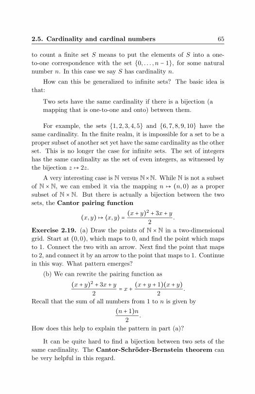
2.5. Cardinality and cardinal numbers 65
to count a finite set S means to put the elements of S into a one-
to-one correspondence with the set {0, . . . , n − 1}, for some natural
number n. In this case we say S has cardinality n.
How can this be generalized to infinite sets? The basic idea is
that:
Two sets have the same cardinality if there is a bijection (a
mapping that is one-to-one and onto) between them.
For example, the sets {1, 2, 3, 4, 5} and {6, 7, 8, 9, 10} have the
same cardinality. In the finite realm, it is impossible for a set to be a
proper subset of another set yet have the same cardinality as the other
set. This is no longer the case for infinite sets. The set of integers
has the same cardinality as the set of even integers, as witnessed by
the bijection z ↦ 2z.
A very interesting case is N versus N×N. While N is not a subset
of N × N, we can embed it via the mapping n ↦ (n, 0) as a proper
subset of N × N. But there is actually a bijection between the two
sets, the Cantor pairing function
(x, y) ↦ ⟨x, y⟩ = (x + y)2 + 3x + y
2.
Exercise 2.19. (a) Draw the points of N × N in a two-dimensional
grid. Start at (0, 0), which maps to 0, and find the point which maps
to 1. Connect the two with an arrow. Next find the point that maps
to 2, and connect it by an arrow to the point that maps to 1. Continue
in this way. What pattern emerges?
(b) We can rewrite the pairing function as
(x + y)2 + 3x + y
2= x + (x + y + 1)(x + y)
2.
Recall that the sum of all numbers from 1 to n is given by
(n + 1)n2
.
How does this help to explain the pattern in part (a)?
It can be quite hard to find a bijection between two sets of the
same cardinality. The Cantor-Schroder-Bernstein theorem can
be very helpful in this regard.

66 2. Infinite Ramsey theory
Theorem 2.20. If there is an injection f ∶ X → Y and an injection
g ∶ Y → X, then X and Y have the same cardinality.
You can find a proof in [35]. You can of course try proving it
yourself, too.
Exercise 2.21. Use the Cantor-Schroder-Bernstein theorem to show
that R and [0, 1] have the same cardinality.
Being able to map a set bijectively to another set is another im-
portant example of an equivalence relation (see Section 1.2). Let us
write
A ∼ B∶ ⇔ there exists a bijection π ∶ A → B.
Exercise 2.22. Show that ∼ is an equivalence relation, that is, it is
reflexive, symmetric, and transitive.
We could define the cardinality of a set to be its equivalence class
with respect to ∼. (This would indeed be a proper class, not a set.)
While this is mathematically sound, it makes thinking about and
working with cardinalities rather cumbersome.
One way to overcome this is to pick a canonical representative for
each equivalence class and then study the system of representatives.
In the case of cardinalities, what should be our representatives?
For finite sets, we use natural numbers. For infinite sets, we can
try to use ordinals, as they continue the counting process beyond the
finite realm. Counting, in this generalized sense, means establishing a
bijection between the set we are counting and an ordinal. If we assume
the axiom of choice, the well-ordering principle ensures that every set
can be well-ordered, so every set would have a representative. The
only problem is that an infinite set can be well-ordered in more than
one way.
Consider for instance the set of integers, Z. We can well-order Z
as follows:
0 < 1 < −1 < 2 < −2 < 3 < ⋯.
This gives a well-ordering of order type ω. But we could also proceed
like this:
1 < −1 < 2 < −2 < 3 < −3 < ⋅ ⋅ ⋅ < 0,

2.5. Cardinality and cardinal numbers 67
that is, we put 0 on top of all other numbers. This gives a well-
ordering of order type ω+1. Or we could put all the negative numbers
on top of the positive integers:
0 < 1 < 2 < 3 < ⋅ ⋅ ⋅ < −1 < −2 < −3 < ⋯,
which gives a well-ordering of type ω + ω.
This implies, in particular, that ω, ω + 1, and ω + ω all have
the same cardinality. Recall that we identify ordinals with their
initial segment, i.e. we put β = {α ∈ Ord∶ α < β}. Hence ω + 1 ={0, 1, 2, . . . , ω}, and we can map ω + 1 bijectively to ω as follows
ω ↦ 0, 0 ↦ 1, 1 ↦ 2, . . .
Exercise 2.23. Show that ωω has the same cardinality as ω.
To obtain a unique representative for each cardinality, we pick
the least ordinal in each equivalence class. (Here it comes in very
handy that the ordinals are well-ordered.)
Definition 2.24. An ordinal κ is a cardinal if for all ordinals β < κ,
β ≁ κ.
For example, ω + 1 is not a cardinal, while ω is—every ordinal
below ω is finite and hence not of the same cardinality as ω. Thus, ω
enjoys a special status in that it is the first infinite cardinal.
Exercise 2.25. Show that every cardinal greater than ω is a limit
ordinal.
To define the cardinality of a set S, denoted by ∣S∣, we now
simply pick out the one ordinal among all possible order types of S
that is a cardinal
∣S∣ = min{α∶ there exists a well-ordering of S of order type α}= the unique cardinal κ such that S ∼ κ.
Note that this definition uses the axiom of choice, since we have
to ensure that each set has at least one well-ordering.
Exercise 2.26. Show that ∣A∣ ≤ ∣B∣ if and only if there exists a one-
to-one mapping A → B.

68 2. Infinite Ramsey theory
How many cardinals are there? Infinitely many. This is Cantor’s
famous theorem.
Theorem 2.27. For every set S, there exists a set of strictly larger
cardinality.
Proof. Consider P(S) = {X ∶X ⊆ S}, the power set of S. The map-
ping S → P(S) given by s ↦ {s} is clearly injective, so ∣S∣ ≤ ∣P(S)∣.We claim that there is no bijection f ∶ S → P(S). Suppose there
were such a bijection f , that is, in particular,
P(S) = {f(x)∶ x ∈ S}.
Every subset of S is the image of an element of S under f . To get
a contradiction, we exhibit a set X ⊆ S for which this is impossible,
namely by letting
x ∈ X ∶⇔ x ∉ f(x).Now, if there were x0 ∈ S such that f(x0) = X, then, by the definition
of X,
x0 ∈ X ⇔ x0 ∉ f(x0) ⇔ x0 ∉ X,
a contradiction. This is a set-theoretic version of Cantor’s diagonal
argument. �
The power set operation always yields a set of higher cardinality.
But by how much? Since the ordinals are well-ordered, so are the
cardinals. We can therefore define, for any cardinal κ,
κ+ = the least cardinal greater thanκ.
Cardinal arithmetic. We now define the basic arithmetic opera-
tions on cardinals. Given cardinals κ and λ, let A and B be sets such
that ∣A∣ = κ, ∣B∣ = λ, and A ∩ B = ∅. Let
κ + λ = ∣A ∪ B∣,(2.2)
κ ⋅ λ = ∣A × B∣,(2.3)
κλ = ∣AB ∣ = ∣{f ∶ f maps B to A}∣.(2.4)
Exercise 2.28. Verify that the definitions above are independent of
the choice of A and B.

2.5. Cardinality and cardinal numbers 69
The power operation 2κ is particularly important because it co-
incides with the cardinality of the power set of κ:
2κ = cardinality of P(κ).
In some ways, cardinal arithmetic behaves just like the familiar
arithmetic of real numbers.
Exercise 2.29. Let κ,λ, and μ be cardinals. Show that
(κλ)μ = κλ⋅μ.
But in other regards, cardinal arithmetic is very different.
Proposition 2.30. Let κ and λ be infinite cardinals. Then
κ + λ = κ ⋅ λ = max{κ,λ}.
Exercise 2.31. Prove Proposition 2.30.
Note that for many arguments involving cardinals and cardinal
arithmetic, the axiom of choice is needed.
Alephs and the continuum hypothesis. Let us denote the car-
dinality of N by ℵ0, i.e. any countable, infinite set has cardinality ℵ0.
Pronounced “aleph”, ℵ is the first letter of the Hebrew alphabet. The
cardinal ℵ0 is the smallest infinite cardinal. We know that the real
numbers R are uncountable, i.e. ∣R∣ > ℵ0, and it is not hard to show
(identifying reals with their binary expansions, which in turn can be
interpreted as characteristic functions of subsets of N) that ∣R∣ = 2ℵ0 .
But is the cardinality of the reals actually the smallest uncountable
cardinality? That is, is it true that
ℵ+0 = 2ℵ0?
This is the continuum hypothesis (CH). Like the axiom of choice,
the continuum hypothesis is independent over the most common ax-
iom system for set theory, ZF. This means that the continuum hy-
pothesis can be neither proved nor disproved in this axiom system.
We will say more about independence in Chapter 4.
Since every cardinal has a successor cardinal (just like ordinals),
we can use ordinals to index cardinals: We let
ℵ1 = ℵ+0 ,

70 2. Infinite Ramsey theory
and more generally, for any ordinal α,
ℵα+1 = ℵ+α.We use ωα instead of ℵα to denote the order type of the cardinal ℵα.
If λ is a limit ordinal, we define
ℵλ = sup{ωα∶α < λ}.
Exercise 2.32. Show that αλ as defined above is indeed a cardinal.
In other words, if S is a set of cardinals, so is the supremum of S.
Exercise 2.33. Show that every cardinal is an aleph, i.e. if κ is a
cardinal, then there exists an ordinal α such that κ = ℵα.
Generalized continuum hypothesis (GCH):
For any α, ℵα+1 = 2ℵα .
If the GCH is true, it means that cardinalities are neatly aligned
with the power set operation. The beth function ℶα is defined
inductively as
ℶ0 = ℵ0, ℶα+1 = 2ℶα , ℶλ = sup{ℶα∶α < λ} for λ a limit ordinal.
That is, ℶα enumerates the cardinalities obtained by iterating the
power set operation, starting with N. If the GCH holds, then ℶα = ℵα
for all α.
2.6. Ramsey theorems for uncountable cardinals
Equipped with the notion of a cardinal, we can now attack the ques-
tion of whether Ramsey’s theorem holds for uncountable sets. It also
makes sense now to consider colorings with infinitely many colors—
the corresponding Ramsey statements are not trivially false anymore.
We will also look at colorings of sets of infinite tuples over a set.
It is helpful to extend the arrow notation for these purposes.
Recall that N �→ (k)pr means that every r-coloring of [N]p has a
monochromatic subset of size k. This is really a statement about
cardinalities, which we can extend from natural numbers to cardinals.
Let κ,μ, η, and λ be cardinals, where μ, η ≤ κ.
κ �→ (η)μλ

2.6. Ramsey theorems for uncountable cardinals 71
means:
If ∣X ∣ ≥ κ and c ∶ [X]μ → λ, then there exists H ⊆ X with
∣H ∣ ≥ η such that c∣[H]μ is constant.
Here [X]μ is the set of all subsets of X of cardinality μ:
[X]μ = {D∶D ⊆ X and ∣D∣ = μ}.
The following lemma keeps track of the cardinality of [X]μ.
Lemma 2.34. If κ ≥ μ are infinite cardinals and ∣A∣ = κ, then
[A]μ = {D∶D ⊆ A and ∣D∣ = μ}
has cardinality κμ.
Proof. As ∣A∣ = κ, any element of κμ corresponds to a mapping
f ∶ μ → A, which is a subset of μ × A. Moreover, any such f satisfies
∣f ∣ = μ. Hence κμ ≤ ∣[μ × A]μ∣ = ∣[A]μ∣, as ∣μ × A∣ = ∣A∣.On the other hand, we can define an injection [A]μ → Aμ: If
D ⊆ A with ∣D∣ = μ, we can choose a function fD ∶ μ → A whose range
is D. Then the mapping D ↦ fD is one-to-one. �
As ℵ0 is the smallest infinite cardinal, we can now write the infi-
nite Ramsey theorem, Theorem 2.1, as
ℵ0 �→ (ℵ0)pr (for any p, r ∈ N).
Finite colorings of uncountable sets. Does the infinite Ramsey
theorem still hold if we pass to uncountable cardinalities?
Let us try to lift the proof from N to ℵ1. To keep things simple,
let us assume we are coloring pairs of real numbers with two colors.
In the proof of ℵ0 �→ (ℵ0)22, one proceeds by constructing a sequence
of natural numbers
z0, z1, z2, . . .
along with a sequence of sets
N = Z0 ⊇ Z1 ⊇ Z2 ⊇ ⋯

72 2. Infinite Ramsey theory
such that
● zi ∈ Zi;
● for each i, the color of {zi, zj} is the same for all j > i; and
● each Zi is infinite.
It was possible to find these sequences because of the simple in-
finite pigeonhole principle: If we partition an infinite set into finitely
many parts, one of them must be infinite.
This principle still holds for uncountable sets: Any finite partition
of an uncountable set must have an uncountable part. In fact, we have
something stronger:
In any partition of an uncountable set into countably many
parts, one of the parts must be uncountable.
Using the language of cardinals, we can state and prove a formal
version of this principle.
Proposition 2.35. If κ is an uncountable cardinal and f ∶ κ → ω,
then there exists an α < ω such that ∣f−1({α})∣ = ℵ1.
Proof. Assume for a contradiction that κα = ∣f−1({α})∣ is countablefor all α < ω. Then
κ = ⋃α<ω
κα
would be a countable union of countable sets, which is countable—a
contradiction. �
Looking at the countable infinite case, one might conjecture that
an even stronger pigeonhole principle should be true, namely that
there is an α such that ∣f−1({α})∣ = κ. This is not quite so; it touches
on an aspect of cardinals called cofinality. We will learn more about
it when we look at large cardinals.
The pigeonhole principle is one instance where uncountable car-
dinals can behave rather differently from ℵ0. We will see that this
has consequences for Ramsey’s theorem.
We return to Ramsey’s theorem and try to prove ℵ1 �→ (ℵ1)22.We start with the usual setup. We choose z0 ∈ ℵ1 and look at all
z ∈ ℵ1∖{z0} such that {z0, z} is red. If the set of such z is uncountable,

2.6. Ramsey theorems for uncountable cardinals 73
then we put Z1 = {z∶ c(z0, z) = red}. Otherwise, by the uncountable
pigeonhole principle, {z∶ c(z0, z) = blue} is uncountable, and we let Z1
be this set. We can now continue as usual inductively and construct
the sequences z0, z1, z2, . . . and Z1 ⊇ Z2 ⊇ Z3 ⊇ ⋯, where each Zi
is uncountable. In the countable case, we were almost done, since it
took only one more application of the (countable) pigeonhole principle
to select an infinite homogeneous subsequence from the zi. Now,
however, we cannot do this, since we are looking for an uncountable
homogeneous set. We therefore need to continue our sequence into
the transfinite. How can this be done? We need to choose a “next”
element of our sequence. We have learned in Section 2.4 that ordinals
are made for exactly that purpose. Hence we would index the next
element by zω. But what should the corresponding set Zω be? We
required Z1 ⊇ Z2 ⊇ Z3 ⊇ ⋯, and hence we should have that
Z1 ⊇ Z2 ⊇ Z3 ⊇ ⋅ ⋅ ⋅ ⊇ Zω.
The only possible choice would therefore be
Zω = ⋂i
Zi.
But this is a problem, because the intersection of countably many
uncountable nested sets is not necessarily uncountable. Consider for
instance the intersection of countably many open intervals
⋂n
(0, 1/n),
which is empty. Indeed, this obstruction is not a coincidence.
Proposition 2.36. Ramsey’s theorem does not hold for the real num-
bers:
∣R∣ = 2ℵ0 /�→ (2ℵ0)22.
We will, in fact, show something slightly stronger:
2ℵ0 /�→ (ℵ1)22.
Of course, if the continuum hypothesis holds, this is equivalent to the
previous statement.
Proof. The proof is based on the fact that a well-ordering of R must
look very different from the usual ordering of the real line.

74 2. Infinite Ramsey theory
Using the axiom of choice, let ≺ be any well-ordering of R. Hence
we can write
R = {x0 ≺ x1 ≺ ⋅ ⋅ ⋅ ≺ xα ≺ xα+1 ≺ ⋯} with all α < 2ℵ0 .
We define a coloring c ∶ [R]2 → {red, blue}. Let y ≠ z be real
numbers and denote the usual ordering of R by <R. Let
c(y, z) =⎧⎪⎪⎨⎪⎪⎩
red if (y <R z and y ≺ z) or (z <R y and z ≺ y),blue otherwise.
Here <R denotes the usual order of R. In other words, we color a set
{y, z} red if the two orderings <R and ≺ agree for y and z. If they
differ, we color the pair blue.
Assume for a contradiction that H is a homogeneous subset for
c of size ℵ1. We can write H as
H = {xα0≺ xα1
≺ ⋅ ⋅ ⋅ ≺ xαξ≺ ⋯} with ξ < ℵ1.
If c↾[H]2≡ red, then we have by definition of c that also
xα0<R xα1
<R ⋅ ⋅ ⋅ <R xαξ<R ⋯,
that is, H gives us a <R-increasing sequence of length ℵ1. If c↾[H]2≡blue, then we get a <R-decreasing sequence of length ℵ1.
We claim that there cannot be such a sequence.
The rationals are dense in R with respect to <R, i.e. between
any two real numbers is a rational number (not equal to either of
them). If there were a strictly <R-increasing or strictly <R-decreasing
sequence of length ℵ1, there would also have to be a strictly <R-
increasing/decreasing sequence of rational numbers of length ℵ1, but
this is impossible, since the rationals are countable. �
The essence of the proof lies in the fact that a homogeneous set
would “line-up” the well-ordering ≺ with the standard ordering <R of
R. If this line-up is too long (uncountable), we get a contradiction
due to the fact that R contains Q as a dense “backbone” (under <R).
The proof also links back to the difficulties encountered earlier
when trying to lift Ramsey’s theorem to 2ℵ0 .

2.6. Ramsey theorems for uncountable cardinals 75
We are dealing with two orderings here: a well ordering ≺ of R
and the familiar linear ordering <R of the real line. Let us call the
first one the “enumeration” ordering, since it determines the order
in which we enumerate R and which element we choose next during
our attempted construction—the ≺-least available. We do not know
much about this ordering other than that it is a well-ordering. (In
fact, there are some metamathematical issues that prevent us from
proving that any explicitly defined function from R to an ordinal is a
bijection.)
The standard ordering <R, on the other hand, is the “color” or-
dering, since going up or down along it determines whether we color
red or blue.
Let us try to follow the construction of a homogeneous set in
the proof of Theorem 2.1 and see where it fails for coloring c. Pick
the ≺-first element of Z0 = R, say xα0. Next check whether the set
{y∶ c(xα0, y) = red} is uncountable. This is the case, since there are
uncountably many y “to the right” of xα0, and also uncountably many
y not yet enumerated (these appear after xα0in the well-ordering).
Hence we put Z1 = {y∶ c(xα0, y) = red} and repeat the argument
for Z1: Pick the ≺-least element of Z1 (which must exist since ≺ is
a well-ordering) and observe that {y ∈ Z1∶ c(xα0, y) = red} is again
uncountable. Inductively, we construct an increasing sequence
xα0<R xα1
<R xα2<R ⋯
and a nested sequence of sets
Z0 ⊃ Z1 ⊃ Z2 ⊃ ⋯
such that
(xαn,∞) ⊇ Zn+1.
But if xαn→ ∞ (which might well be the case), this implies
⋂n
Zn = ∅,
and hence after ω-many steps we cannot continue our construction.
We could try to select the αn a little more carefully; in particular,
we could, for instance, let xαn+1be the ≺-least element of Zn+1 such
that xαn<R xαn+1
< xαn+1/2n. This way we would guarantee that we

76 2. Infinite Ramsey theory
could continue our construction beyond stage ω and into the transfi-
nite. In fact, by choosing the xα carefully enough, we can ensure that
the construction goes on for β-many stages for any fixed countable
ordinal β. But the cardinality argument of the proof above tells us it
is impossible to do this for ℵ1-many stages.
Exercise 2.37. Show that Proposition 2.36 generalizes to
2κ /�→ (κ+)22.
(Hint: Show that {0, 1}κ has no increasing or decreasing sequence of
length κ+.)
An obvious question now arises: If we allow higher cardinalities κ
beyond 2ℵ0 , does κ → (ℵ1)22 become true eventually? The Erdos-Rado
theorem shows that we in fact only have to pass to the next higher
cardinality.
Theorem 2.38 (Erdos-Rado theorem).
(2ℵ0)+ �→ (ℵ1)22.
Compared to the counterexample in Proposition 2.36, the extra
cardinal gives us some space to
set aside an uncountable set such that whenever we extend
our current homogeneous set, we leave this set untouched,
i.e. we do not add elements from it.
In this way, we can now guarantee that the sets Zα will have a non-
empty, in fact uncountable, intersection.
This “setting aside” happens by virtue of the following lemma.
Lemma 2.39. There exists a set R ⊂ (2ℵ0)+ of cardinality ∣R∣ = 2ℵ0
such that for every countable D ⊆ R and for every x ∈ (2ℵ0)+ ∖ D,
there exists an r ∈ R ∖ D such that for all d ∈ D,
(2.5) c(x, d) = c(r, d).
Informally, whenever we choose an x and a countable D ⊂ R, we
can find a “replacement” for x in R that behaves in a color-identical
manner with respect to D. This will enable us, in our construction

2.6. Ramsey theorems for uncountable cardinals 77
of a homogeneous set of size ℵ1, to choose the xα from a set of size
2ℵ0 , leaving a “reservoir” of uncountable cardinality.
Proof. We construct the set R by extending it step by step, adding
the witnesses required by (2.5).
We start by putting R0 = 2ℵ0 . We have to ensure that (2.5) holds
for every countable subset D ⊂ R0 and every x ∈ (2ℵ0)+ ∖ D. To
simplify notation, let us put
cx(y) = c(x, y).
Hence every x fixes a function cx ∶ (2ℵ0)+ ∖ {x} → {0, 1}. We are
interested in the functions cx ↾D for countable D ⊂ R0. Each such
function maps a countable subset of R0 to {0, 1}.We count the number of such functions. If we fix a countable
D ⊂ R0, there are at most 2ℵ0-many ways to map D to {0, 1}. By
Lemma 2.34, there are
(2ℵ0)ℵ0 = 2ℵ0 ⋅ℵ0 = 2max{ℵ0,ℵ0} = 2ℵ0
countable subsets of 2ℵ0 . Therefore, there are at most
2ℵ0 ⋅ 2ℵ0 = 2ℵ0
possible functions cx↾D. (Note that while each x ∈ (2ℵ0)+ gives rise
to such a function, many of them will actually be identical, by the
pigeonhole principle.)
Therefore, we need to add at most 2ℵ0-many witnesses to R0,
one r ∈ (2ℵ0)+ for each function cx↾D (of which there are at most 2ℵ0-
many). This gives us R1, and R1 in turn gives rise to new countable
subsets D which we have to witness by possibly adding new elements
from (2ℵ0)+ to R1. But the crucial fact here is that the cardinality
of R1 is still 2ℵ0 , since 2ℵ0 + 2ℵ0 = 2ℵ0 , and therefore we can resort
to the same argument as before, adding at most 2ℵ0-many witnesses,
resulting in a set R2 of cardinality 2ℵ0 .
We have to run our construction into the transfinite. Let α be a
countable ordinal, and assume that we have defined sets
R0 ⊆ R1 ⊆ ⋅ ⋅ ⋅ ⊆ Rβ ⊆ ⋯

78 2. Infinite Ramsey theory
for all β < α, ∣Rβ ∣ = 2ℵ0 . If α is a successor ordinal, α = β+1, we define
Rα by the argument given above, adding at most 2ℵ0 new witnesses.
If α is a limit ordinal, we put
Rα = ⋃β<α
Rβ.
This is a countable union of sets of cardinality 2ℵ0 , and hence is also
of cardinality 2ℵ0 (see Proposition 2.30).
Finally, put
R = ⋃α<ω1
Rα.
We claim that this R has the desired property. First note that the
cardinality of R is
ℵ1 ⋅ 2ℵ0 = max{ℵ1, 2ℵ0} = 2ℵ0 .
LetD ⊂ R be countable and let x ∈ (2ℵ0)+∖D. The crucial observation
is that
all elements ofD must have been added by some stage α < ω1,
i.e. there exists an α < ω1 such that D ⊆ Rα.
If this were not the case, every stage would add a new element of D,
which would mean D has at least ω1-many elements, in contradiction
to D being countable. But then the necessary witness for cx ↾D is
present in Rα+1; that is, there exists an r ∈ Rα+1 ⊆ R such that
cr ↾D= cx ↾D.
This completes the proof of the lemma. �
We can now use the lemma to modify our construction of a ho-
mogeneous set H.
Proof of the Erdos-Rado theorem. Let x∗ be an arbitrary ele-
ment of (2ℵ0)+ ∖ R. This will be our “anchor point”. Choose x0 ∈ R
arbitrary.
Suppose now, given α < ω1, we have chosen xβ for all β < α.
Let
D = {xβ ∶β < α}.This is a countable set (since α < ω1). By Lemma 2.39, there exists
an r ∈ R such that cx∗ ↾D= cr ↾D. Put xα = r.

2.6. Ramsey theorems for uncountable cardinals 79
By the pigeonhole principle, there exists i ∈ {0, 1} such that
H = {xα∶ α < ω1, c(x∗, xα) = i}
is uncountable. We claim that c↾[H]2≡ i, i.e. H is homogeneous for c.
For suppose xζ , xξ ∈ H and ζ < ξ. Then, by definition of xξ,
c(xξ, xζ) = cξ(xζ) = cx∗(xζ) = c(x∗, xα) = i.
�
Note that the proof becomes quite elegant once we have proved
the lemma. After we ensured the existence of the set R, we can work
in some sense “backwards”: We choose a single “anchor point” x∗
from the reserved set (2ℵ0)+∖R. You can think of x∗ as always being
the next point chosen in the sense of the standard construction, only
then to be replaced by an element from R which behaves exactly like
it in terms of color pairings with the already constructed xβ .
Note also that we do not need to construct a sequence of shrinking
sets Zα anymore. In the standard construction, the Zα represent the
reservoir from which the next potential elements of the homogeneous
set are chosen. They are no longer needed since x∗ is always available
(as explained above).
We also do not need to keep track of the color choices we made
along the way, as x∗ does this job for us, too. For example, if
c(x∗, x0) = 0, it follows by construction that c(xβ , x0) = 0 for all
β > 0, which in the previous constructions means that we restrict the
Z to all elements which color 0 with x0.
Exercise 2.40. Generalize the proof of the Erdos-Rado theorem (and
Lemma 2.39) to show that
ℶ+n �→ (ℵ1)n+1ℵ0 .
Infinite colorings. The Erdos-Rado theorem holds for countable
colorings, too (see Exercise 2.40). What else can we say about infinite
colorings? Clearly, the number of colors should be smaller than the
set we are trying to color. For example,
ℵ0 /�→ (2)1ℵ0 .

80 2. Infinite Ramsey theory
But even if we make the colored set larger than the number of colors,
this does not mean we can find even a finite homogeneous set.
Proposition 2.41. For any infinite cardinal κ,
2κ /�→ (3)2κ.
Proof. We define c ∶ [2κ]2 → κ as follows. An element of 2κ corre-
sponds to a {0, 1}-sequence (xβ ∶β < κ) of length κ (recall that 2κ is
the cardinality of the power set of κ, and every element of the power
set can be coded by its characteristic sequence; (xβ ∶β < κ) is such a
characteristic sequence). Given two such sequences (xβ) ≠ (yβ), welet
c((xβ), (yβ)) = the least α < κ such that xα ≠ yα.
Now assume that (xβ), (yβ), (zβ) are pairwise distinct. Let c((xβ),(yβ)) = α. Without loss of generality, xα = 0 and yα = 1. Now zα ∈{0, 1}, so either zα = xα or zα = yα. In the first case c((xβ), (zβ)) ≠ α
and in the second case c((yβ), (zβ)) ≠ α. Therefore, there cannot
exist a c-homogeneous subset of size 3. �
2.7. Large cardinals and Ramsey cardinals
The results of the previous section make the set of natural numbers
stand out among the infinite sets not only because ℵ0 is the first
infinite cardinal but also for another reason: With respect to finite
colorings of finite tuples, the natural numbers admit a homogeneous
subset of the same size, or, in the Ramsey arrow notation,
ℵ0 �→ (ℵ0)prfor any positive integers p and r.
In the previous section, we saw that this is no longer true for ℵ1
(Proposition 2.36). In fact, for any infinite cardinal κ,
2κ /�→ (κ+)22,so in particular
2κ /�→ (2κ)22for any infinite cardinal κ.
This in turn means that any cardinal λ that can be written as λ =2κ cannot satisfy λ �→ (λ)22. But are there any cardinals that cannot

2.7. Large cardinals and Ramsey cardinals 81
be written this way? ℵ0, the cardinality of N, is such a cardinal—the
power set of a finite set is still finite. But other than N?
Definition 2.42. A cardinal λ is a limit cardinal if λ = ℵγ for some
limit ordinal γ. λ is a strong limit cardinal if for all cardinals κ < λ,
2κ < λ.
Any strong limit cardinal is a limit cardinal. For if λ is a succes-
sor cardinal, then λ = ℵα+1 = ℵ+α ≤ 2ℵα . Is being strong limit truly
stronger than being limit? Well, it depends. If the GCH holds, then
2ℵα = ℵ+α = ℵα+1 for all α, and therefore every limit cardinal is actually
a strong limit cardinal.
For now just let us assume that κ is a strong limit cardinal. Is
this sufficient for
κ �→ (κ)22 ?Take for example ℵω. This is clearly a limit cardinal and, if the GCH
holds, also a strong limit cardinal. Does it hold that
ℵω �→ (ℵω)22?The problem is that we can “reach” ℵω rather “quickly” from below,
since
ℵω = ⋃n<ω
ℵn.
We can use this fact to devise a coloring of ℵω that cannot have a
homogeneous subset of size ℵω. Namely, let us put, for each n < ω,
Xn+1 = ℵn+1 ∖ ℵn.
Then ℵω is the disjoint union of the Xn, and the cardinality of each
Xn is strictly less than ℵω. Now define a coloring c ∶ [ℵω]2 → {0, 1}by
c(x, y) =⎧⎪⎪⎨⎪⎪⎩
1 if x and y are in different Xn,
0 if x and y are in the same Xn.
Let H ⊂ ℵω be a homogeneous subset for c. If c↾[H]2≡ 1, then no two
elements of H can be in the same Xn, but there are only ℵ0-many
Xn, and hence H is countable. If c ↾[H]2≡ 0, then all elements of H
have to be in the same Xn, but as noted above, ∣Xn∣ < ℵω for each n.
The proof works in general for any cardinal κ that we can reach
in fewer than κ steps. This brings us to the notion of cofinality.

82 2. Infinite Ramsey theory
Definition 2.43. The cofinality of a limit ordinal α, cf(α), is the
least ordinal β such that there exists an increasing sequence (αγ)γ<βof length β such that αγ < α for all α and
α = limγ→β
αγ = sup{ξγ ∶γ < β}.
Obviously, we always have cf(α) ≤ α. Here are some examples as
an exercise.
Exercise 2.44. Prove the following cofinalities:
(i) cf(ω) = ω,
(ii) cf(ω + ω) = ω,
(iii) cf(α) = ω for every countable, infinite α,
(iv) cf(ω1) = ω1 (if we assume AC),
(v) cf(ωω) = ω.
The last statement can be generalized to
cf(ωλ) = cf(λ),
where λ is any limit ordinal.
If κ is an infinite cardinal and cf(κ) < κ, it means that κ can
be reached from below by means of a “ladder” that has fewer steps
than κ. Such a cardinal is called singular. If cf(κ) = κ, κ is called
regular. Hence ℵ0 and ℵ1 are regular cardinals, while ℵω is singular.
Assuming the axiom of choice, one can show that every successor
cardinal, that is, a cardinal of the form ℵα+1, is a regular cardinal.
It seems much harder for a limit cardinal to be regular. For this
to be true, the following must hold:
ℵλ = cf(ℵλ) = cf(λ) ≤ λ.
But since clearly ℵλ ≥ λ, this means that
if ℵλ is regular (λ limit), then ℵλ = λ.
This seems rather strange. Going, for example, from ℵ0 to ℵ1, we
traverse ω1-many ordinals, but the jump “costs” only one step in
terms of cardinals. That means we have to go a long, long way if we
ever want to “catch up” with the alephs again.

2.7. Large cardinals and Ramsey cardinals 83
Anyway, let us capture the notions of large cardinals we have
found so far in a formal definition.
Definition 2.45. Let κ be an uncountable cardinal.
(i) κ isweakly inaccessible if it is regular and a limit cardinal.
(ii) κ is (strongly) inaccessible if it is regular and a strong
limit cardinal.
(iii) κ is Ramsey if κ �→ (κ)22.
Usually, strongly inaccessible cardinals are called simply inacces-
sible. Our investigation leading up to Definition 2.45 now yields the
following.
Theorem 2.46. Every Ramsey cardinal is inaccessible.
Do Ramsey cardinals exist? We cannot answer this question here,
nor will we in this book. In fact, in a certain sense we cannot answer
this question at all. More precisely, the existence of Ramsey cardinals
cannot be proved in ZF. As mentioned before in Section 2.5, ZF is a
common axiomatic framework for set theory in which most of con-
temporary mathematics can be formalized. We will say more about
axiom systems and formal proofs in Chapter 4.


Chapter 3
Growth of Ramseyfunctions
3.1. Van der Waerden’s theorem
In this chapter, we return from the infinite realm to the finite, but we
will see how we can approximate the infinite through really big finite
numbers. This may sound absurd, but will hopefully make some sense
by the end of Chapter 4.
We have seen in Chapter 1 that the diagonal Ramsey numbers
R(n) = R(n,n) grow rather fast. Nobody knows how fast exactly,
but the upper and lower bounds proved in Chapter 1 tell us that the
growth is exponential of some sort. Loosely speaking, there has to be
a lot of chaos to guarantee the existence of a little bit of order inside.
It turned out that many other results in Ramsey theory exhibit
a similar behavior. Arguably the most famous theorem of this kind
(which actually preceded Ramsey’s theorem by a few years) is van
der Waerden’s theorem on arithmetic progressions [68]. We will see,
in fact, that the analysis of the associated van der Waerden numbers
gives rise to an interesting metamathematical perspective.
An arithmetic progression (AP) of length k is a sequence of
the form
a, a + m, a + 2m, . . . , a + (k − 1)m,
85

86 3. Growth of Ramsey functions
where a and m are integers. We will call arithmetic progressions of
length k simply k-APs.
Theorem 3.1 (Van der Waerden’s theorem). Given integers r, k ≥ 1,
for any r-coloring of N there exists a monochromatic k-AP.
In other words, in any finite coloring of the natural numbers we
can find arithmetic progressions of arbitrary length. It is important to
be aware that “arbitrary length” here means “arbitrary finite length”.
It is not true that any finite coloring of N has a monochromatic arith-
metic progression of infinite length.
Exercise 3.2. Construct a 2-coloring of N such that neither color
contains an infinite arithmetic progression.
(Hint: Alternate between longer and longer blocks of 1’s and 2’s.)
The exact location of the first k-AP will of course depend on
the particular coloring. It is, however, possible to bound this first
occurrence from above a priori, that is, independent of any coloring.
Theorem 3.3 (Van der Waerden’s theorem, finite version). Given
integers r, k ≥ 1, there exists a number W such that any r-coloring of
{1, . . . ,W} has a monochromatic k-AP.
The smallest possible W is called the van der Waerden num-
ber for k and r, and in the following we will denote it by W (k, r).That the finite version is a consequence of the first version is
not completely obvious. It could be that for every n, we could find
one specific coloring of {1, . . . , n} such that no monochromatic k-AP
exists for that coloring. However, we could, as in the proof of the finite
Ramsey theorem via compactness, collect these examples in a tree and
find an infinite path, yielding a coloring of N. A similar argument to
that in the Ramsey case would then yield a contradiction.
Exercise 3.4. Give a detailed derivation of the finite version of van
der Waerden’s theorem from Theorem 3.1 using compactness. Follow
the template outlined at the end of Section 2.2.

3.1. Van der Waerden’s theorem 87
Van der Waerden himself gave a wonderful account of how he (to-
gether with E. Artin and O. Schreier) found the proof of the theorem
that now bears his name [69,70]. We will try to follow his exposition
here.
“Start with the very simple examples” (Hilbert).
One easily sees that W (2, r) = r + 1. Any two numbers x and
y form an arithmetic progression of length 2, by setting a = x and
m = y − x. Thus, to have a monochromatic 2-AP it suffices to have
two numbers of the same color. But by the pigeonhole principle, any
r-coloring of {1, . . . , r+1} has at least two numbers of the same color.
And we also see that the bound r + 1 is optimal in this case.
As the case of r = 2 and k = 3 is not nearly as simple, van der
Waerden first checked some cases by hand (literally using pencil and
paper, we have to guess, as the year was 1927 and no computers were
available). He found a 2-coloring of {1, . . . , 8} that does not have a
monochromatic 3-AP (Figure 3.1):
blue
red
1 2 3 4 5 6 7 8
Figure 3.1. A coloring of {1, . . . ,8} with no monochromatic 3-AP1
But then he saw that no matter how you color {1, . . . , 9} (29 =512 possible colorings), there will always be a monochromatic 3-AP.
In other words, W (3, 2) = 9. Keep in mind, though, that van der
Waerden was originally trying to prove Theorem 3.1, not the finite
version, Theorem 3.3. As we outlined above, the mere existence of
W (3, 2) is not clear at all from the statement of Theorem 3.1. But
the three mathematicians were able to deduce Theorem 3.3 given
that Theorem 3.1 holds by an argument similar to the compactness
argument we have used. (They did not call it compactness though.)
1Our diagrams follow the design of van der Waerden [69]. In the case of twocolors, the top line will always represent the color blue and the bottom one always red.

88 3. Growth of Ramsey functions
Two colors versus many.
Artin, Schreier, and van der Waerden thenceforth tried to prove
the existence of the numbers W (k, r) through induction. Artin re-
marked that the finite version of the theorem made an induction ap-
proach easier, since one could use the existence of W (k, r), which is
a specific natural number, in an attempt to establish the existence of
W (k + 1, r).Artin made another key observation:
(3.1) If W (k, 2) exists for every k, then W (k, r) exists for all r and
k.In other words, if we know that the finite theorem holds for r = 2 and
all k, then it holds for all r and k.
Take for example r = 3 and consider a 3-coloring of N. This in-
duces a 2-coloring if we identify colors 1 and 2. For this 2-coloring we
know there exists a monochromatic arithmetic progression of length
W (k, 2). If the color of this arithmetic progression is 3, then we are
done (since W (k, 2) ≥ k). Otherwise we have a 2-colored arithmetic
progression
a, a + m, a + 2m, . . . , a + (W (k, 2) − 1)m,
not quite what we want yet. But if we renumber the terms of our
progression as 1, 2, 3, . . . , we induce a 2-coloring of {1, . . . ,W (k, 2)}.By definition of W (k, 2) (and the assumption that it exists), there
exists a monochromatic k-AP for this coloring. This k-AP in turn
translates into a monochromatic sub-k-AP of the first progression.
We therefore have shown that W (k, 3) ≤ W (W (k, 2), 2). It should
now be clear how this proof can be continued by induction.
Note, however, that in order to show that W (k, 3) exists, we have
used the existence of W (l, 2) for potentially much larger l. We have
to keep this in mind when we try to prove the existence of W (k, r) by
some form of double induction, as we have to avoid circular arguments
(e.g., using the existence of W (l, 2) to prove the existence of W (k, 3)for k < l, but using W (k, 3) in turn to establish the existence of
W (l, 2)).

3.1. Van der Waerden’s theorem 89
Block progressions.
Being able to use more than two colors turned out to play a crucial
role in establishing the existence of W (k, 2) by induction. The colors
occur as “block colors”, in the following sense. Suppose we have a 2-
coloring of N. For some fixed m ≥ 1, consider now consecutive blocks
of m numbers, i.e.
1, 2, . . . ,m, m+1,m+2, . . . , 2m, 2m+1,m+2, . . . , 3m, . . . .
Every one of those blocks has a corresponding color sequence of
length m. For example, if m = 5, then
or, in short, 1 2 2 1 1
would be a possible color block. There are 2m such potential color
blocks overall. The key idea is to
(3.2) regard an m-block as a single entity and consider these
entities 2m-colored
.
Artin suggested that one could apply an induction hypothesis
for W (k − 1, 2m), that is, the existence of (k − 1)-many m-blocks in
arithmetic progression, each of which has the same m-color pattern.
It was, however, unclear at that point how exactly this might be
helpful.
Van der Waerden’s breakthrough.
Being able to use more than two colors to establish the existence
of W (k, 2) proved crucial for the proof, together with the following
principle, which we applied above:
(3.3) Any arithmetic progression “inside” an arithmetic progres-
sion is again an arithmetic progression.
Let us try to deduce that W (3, 2) exists, by a formal deduction
instead of a brute force argument where we simply check all the cases.
It is helpful to imagine an evil adversary who counters every guess
we make by choosing a coloring that makes it as hard as possible for
us to find monochromatic arithmetic progressions. We have to corner
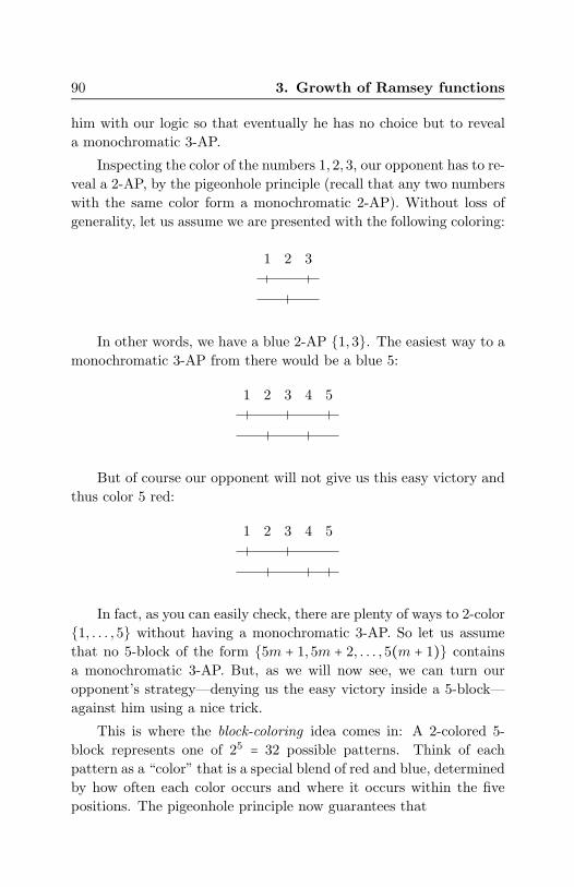
90 3. Growth of Ramsey functions
him with our logic so that eventually he has no choice but to reveal
a monochromatic 3-AP.
Inspecting the color of the numbers 1, 2, 3, our opponent has to re-
veal a 2-AP, by the pigeonhole principle (recall that any two numbers
with the same color form a monochromatic 2-AP). Without loss of
generality, let us assume we are presented with the following coloring:
1 2 3
In other words, we have a blue 2-AP {1, 3}. The easiest way to a
monochromatic 3-AP from there would be a blue 5:
1 2 3 4 5
But of course our opponent will not give us this easy victory and
thus color 5 red:
1 2 3 4 5
In fact, as you can easily check, there are plenty of ways to 2-color
{1, . . . , 5} without having a monochromatic 3-AP. So let us assume
that no 5-block of the form {5m + 1, 5m + 2, . . . , 5(m + 1)} contains
a monochromatic 3-AP. But, as we will now see, we can turn our
opponent’s strategy—denying us the easy victory inside a 5-block—
against him using a nice trick.
This is where the block-coloring idea comes in: A 2-colored 5-
block represents one of 25 = 32 possible patterns. Think of each
pattern as a “color” that is a special blend of red and blue, determined
by how often each color occurs and where it occurs within the five
positions. The pigeonhole principle now guarantees that

3.1. Van der Waerden’s theorem 91
among the first 33 5-blocks (i.e. the numbers {1, . . . , 165}divided into consecutive blocks of 5 numbers), one color (i.e.
5-pattern) must occur twice.
To make the argument more concrete, suppose that the blocks
B8 = {36, 37, 38, 39, 40} and B21 = {101, 102, 103, 104, 105} have the
same 2-coloring pattern. (There is nothing particular about these
two blocks; the argument works just as well for any other pair, with
slightly adjusted numbers.) Now, as above, if we consider only the
color of B8, the pigeonhole principle tells us that two of 36, 37, and 38
must have the same color. Denote these elements by i and j so that
i ∈ {36, 37} and j ∈ {37, 38}. The step-width of this 2-AP is m = j − i.
We also have i+2m ≤ 40, so we could theoretically complete this into
a 3-AP inside B8, but as we said, our opponent will not grant us this
easy victory.
Let us assume, again for illustrative purposes, that i = 36 and
j = 38 are colored blue, while i + 2m = 40 is colored red. B21 has the
same coloring pattern and, depending on how 39 is colored, we might
have the following picture:
B8 B21
36 40 101 105
Figure 3.2. The 5-blocks B8 and B21 have the same coloringpatterns.
The two blocks together still do not give us a 3-AP. But the
picture changes when we consider the 3-AP of 5-blocks generated by
B8, B21, and B34. In other words, we consider a 3-AP of blocks
corresponding to their indices.
Of course, the coloring pattern of B34 might be completely dif-
ferent from that of B8 and B21. But the crucial fact, as simple as it
may sound, is that the last element of B34, 170, is assigned a color.
How would this help us? Let’s look at the three blocks together:

92 3. Growth of Ramsey functions
∣∣
∣∣∣
B8
∣∣
∣∣∣
B21 B34
40 105 170
Figure 3.3. Extending the block-2-AP B8,B21 to a block-3-AP B8,B21,B34
Since the blocks are in arithmetic progression, the numbers inside
the blocks are approximately in arithmetic progression. If we take the
kth number from each block (1 ≤ k ≤ 5), we obtain in fact an exact
arithmetic progression, such as 37, 102, 166 (the second element of
each block). This is the principle stated in (3.3): Any arithmetic pro-
gression inside an arithmetic progression is an arithmetic progression.
But there are other ones: the progression 36, 102, 168, for example,
consisting of the first element of B8, the second of B21, and the third
of B34, or 36, 103, 170 (the first, third, and fifth elements, respec-
tively). The one that matters for us is the one corresponding to the
monochromatic 2-AP in B8 and B21. In our example, this was the
one given by the first and third elements (36 and 38, or 101 and 103,
respectively). Now we “stretch out” this 3-AP over all three blocks:
36, 103, 170.
Is this a monochromatic 3-AP? Not necessarily, as 170 might be
colored red. But in this case 40, 105, 170 is a red 3-AP.
By making 170 the “focal point” of two 3-APs, both of which are
monochromatic in their first two terms (and with different colors),
we have cornered our opponent. No matter what color he chooses for
170, it will complete a monochromatic 3-AP.
∣∣
∣∣∣
B8
∣∣
∣∣∣
B21 B34
40 105 170
Figure 3.4. No matter how 170 is colored, we will get amonochromatic 3-AP: either 36,103,170 (blue) or 40,105,170(red).
3.1. Van der Waerden’s theorem 93
It should be clear how to reproduce this argument for other in-
stances. In particular, we see that in the worst case, we need to
consider the block-3-AP B1,B33,B65. (This is the one that is most
spread out.) In other words, our argument shows that
W (3, 2) ≤ 65 ⋅ 5 = 325.
While this seems a rather large bound considering one can estab-
lish W (3, 2) = 9 by checking all cases, the way we arrived at it can be
generalized to higher orders.
Let us try to capture the essential steps in this argument.
1. Choose a block size. Our block size was 5 since it guaranteed
the existence of a monochromatic 2-AP that can be extended
to a 3-AP (not necessarily monochromatic) within the block.
2. Find an arithmetic progression of block-coloring patterns.
There are 25 = 32 possible 2-colorings of 5-blocks. Hence
among 33 5-blocks, two must be the same. These blocks
form a 2-AP of blocks.
3. Extend the arithmetic progression of block patterns by one
block. The additional block may not have the same coloring
pattern, but we will use it to “force” a monochromatic AP
in the next step.
4. Consider arithmetic progressions of numbers inside the block
progression. One element of the additional block will be the
“focal point” of a monochromatic AP, either by collecting
the elements in each block at a constant position, or by ex-
tending a “diagonal” AP, such as, in our example, elements
1, 3, and 5 from blocks B8, B21, and B34, respectively.
Exercise 3.5. Follow the template above to argue that W (4, 2) ex-
ists. You may assume that all numbers of the form W (3, r) exist. It
helps to make a drawing like we did above.
1. We need a block size that guarantees the existence of a
monochromatic 3-AP that can be extended to a 4-AP (not
necessarily monochromatic). Express this in terms ofW (3, 2).2. Let M be the block size. There are 2M ways to color such a
block. But now we need to find not only two but three blocks

94 3. Growth of Ramsey functions
with an identical color pattern (since we want to extend to a
4-AP). Above we used the pigeonhole principle, but we can
also say we used the existence of W (2, 32) = 33. Which van
der Waerden number W (3, ⋅) would we use in this case?
3. How far would we have to go next to extend this 3-AP of
blocks by one block?
4. Find the focal point of two monochromatic 3-APs and argue
as above that the focal point must extend one of them to a
monochromatic 4-AP.
Working through this example, it hopefully becomes clear how
one can apply the template to show that W (k, 2) exists for an arbi-
trary k, assuming that W (k − 1, r) exists for all r.
Can this method be adapted to show the existence of W (k, r)for r > 2? Before we think about this, did we not show in (3.1) that
once we have proved the result for r = 2, it follows for all r > 2? Yes,
but the crux is that in the proof of (3.1), we needed the existence of
W (W (k, 2), 2) to establish the existence of W (k, 3). And above we
saw that to establish the existence of W (4, 2), we need the existence
of numbers W (3, r). Hence we cannot combine the two proofs, as
it would yield a circular argument. Observation (3.1) only assured
Artin, Schreier, and van der Waerden that an inductive approach
using the block-coloring method was possible, since there would be
no “holes” in the table of numbers W (k, r). But the actual proof of
going from W (k, 2) to W (k, 3) would have to proceed differently to
avoid the circularity outlined above.
We again follow van der Waerden in demonstrating that W (3, 3)exists. We start by choosing a block size that ensures the existence
of a monochromatic 2-AP with a possible extension to a 3-AP. As
we have three colors now, a monochromatic 2-AP will appear among
four numbers instead of three, and to extend it to a 3-AP we need a
block size of 7 instead of 5.
We can apply the previous line of reasoning and get a 3-AP of
blocks, the first two of which have an identical coloring pattern. These
three blocks span, in the worst case, the numbers from 1 to 7 ⋅37 +7+7 ⋅ 37 = 7 ⋅ (2 ⋅ 37 + 1). But the “focal point” argument does not work

3.1. Van der Waerden’s theorem 95
anymore (or at least not right away), since the “focal number” could
now be colored with the third color, say green.
∣∣
∣∣∣
∣∣
∣∣∣
∣
Figure 3.5. Escaping a monochromatic 3-AP by coloring thefocal point green
But we can apply the block argument again—to the big block of
size M = 7 ⋅ (2 ⋅ 37 + 1). There are
3M = 37⋅(2⋅37+1) possible 2-colorings of such a block.
Hence, among 3M + 1 such blocks, we must see two with the same
coloring pattern.
∣∣
∣∣∣
∣∣
∣∣∣
∣
∣∣
∣∣∣
∣∣
∣∣∣
∣
Figure 3.6. A 2-AP of blocks each containing a 3-AP of blocks
And again, they define a 2-AP of blocks. Once more, we extend
this 2-AP to a 3-AP:
∣∣∣∣
∣∣∣∣∣
∣∣
∣∣∣∣
∣∣∣∣∣
∣∣
Figure 3.7. Extending the 2-AP of “big blocks” to a 3-AP
We do not know what the coloring of the third big block is, but
arguing as before, one element in the third (inner) 7-block of the
third (outer) M -block becomes the focal point of three arithmetic
progressions, as indicated in the following picture:

96 3. Growth of Ramsey functions
∣∣∣∣
∣∣∣∣∣
∣∣
∣∣∣∣
∣∣∣∣∣
∣∣
Figure 3.8. Finding a focal point of three different 3-APs
Each of the three arithmetic progressions is monochromatic in
the first two terms, and each has a different color. Hence no matter
what color the focal point is, it will complete a monochromatic 3-AP.
Exercise 3.6. Show that the above argument establishes thatW (3, 3)≤ 5 ⋅ 1014616.
(Hint: 5 ⋅ 1014616 > (2 ⋅ 37⋅(2⋅37+1) + 1) ⋅ (2 ⋅ 37 + 1) ⋅ 7.)
Note that our argument uses only the pigeonhole principle (i.e.
the existence of W (2, r) for r = 3M ). The existence of W (k, r) for
k > 2 and r ≥ 2 is not needed.
Exercise 3.7. Generalize the previous argument to show thatW (3, r)exists for any r ≥ 2. Can you derive a bound for W (3, r)?
Exercise 3.8. Sketch a proof that W (4, 3) exists by combining the
arguments for W (3, 3) and W (4, 2). A careful drawing can represent
most of the argument. What should the initial block size be in this
case? The existence of which numbers W (k, r) do we have to assume?
The general case.
Let us now try to generalize the previous arguments to arbitrary
k, r. The idea remains the same: Find (k − 1)-APs of larger and
larger block patterns, until we can construct a number that is the
“focal point” of r-many (k − 1)-APs, each of a different color.
Formally, we will define a function U(k, r) by recursion, which es-
tablishes an upper bound on W (k, r), using van der Waerden’s tech-
nique. Keep in mind that the actual van der Waerden numbers can
be quite a bit smaller, as we have seen in the case of k = 3 and r = 2:
The actual value is W (3, 2) = 9, while U(3, 2) = 325.
We start with the “innermost” block. For 3-APs, that block size
was determined by taking r + 1 = W (2, r) (i.e. the smallest number

3.1. Van der Waerden’s theorem 97
for which a monochromatic 2-AP exists) and extending it sufficiently
so that we can extend our 2-AP to a 3-AP. In the worst case, our
2-AP is given by the numbers 1 and r + 1, and hence its extension to
a 3-AP would be
1, r + 1, 2r + 1,
which means that the first box size is 2r + 1. In the general case
U(k, r), we start with a (k − 1)-AP over r colors, i.e. the interval
{1, . . . , U(k − 1, r)}, and have to extend it by
⌊U(k − 1, r) − 1
k − 2⌋ .
Hence the block size for the innermost block would be
(3.4) b1 = U(k − 1, r) + ⌊U(k − 1, r) − 1
k − 2⌋ .
Next, we consider coloring patterns of blocks of size b1. There
are rb1 possibilities for each block, so to find a (k−1)-AP of b1-blocks
with the same coloring pattern we need U(k − 1, rb1) of them. By
putting
b2 = U(k − 1, rb1) + ⌊U(k − 1, rb1) − 1
k − 2⌋ ,
we guarantee that among b2 blocks of size b1, there are k blocks in
arithmetic progression, the first k − 1 blocks of which have the same
coloring pattern.
We can now continue inductively. Let
(3.5) bj+1 = U(k − 1, rbj ) + ⌊U(k − 1, rbj ) − 1
k − 2⌋ ,
and put
(3.6) U(k, r) = br ⋯ b2 b1.
Then van der Waerden’s argument yields that
W (k, r) exists and is at most U(k, r).
It hopefully is clear why the argument (and the numbers) work. A
formal proof is a little tedious—a double induction on k and r: Fixing
k, we prove the result (inductively) for all r, and then use this (as we

98 3. Growth of Ramsey functions
do in the definition of the numbers U(k, r)) to prove W (k + 1, 2) ≤U(k + 1, 2).
Arguably the shortest and most elegant proof along the lines of
van der Waerden’s original ideas was given by Graham and Roth-
schild [23]. Another good presentation (with weaker but simpler
bounds) can be found in the book by Khinchin [41].
A density version of van der Waerden’s theorem. Turan’s the-
orem shows that if we assume a certain density of edges, a complete
subgraph of a certain size must be present. One can ask a similar
question for van der Waerden’s theorem: If a color is present with a
certain density, do arithmetic progressions in that color exist? The
answer is yes, and the result is known as Szemeredi’s theorem,
arguably one of the great results of 20th century mathematics.
Theorem 3.9 (Szemeredi’s theorem [64]). Let A ⊂ N. If
lim supn→∞
∣A ∩ {1, 2, . . . , n}∣n
> 0,
then for any k ≥ 1, A contains infinitely many arithmetic progressions
of length k.
We will not prove Szemeredi’s theorem here, but we wanted to
at least state it, as the result has inspired some truly important de-
velopments in mathematics, from Furstenberg’s ergodic-theoretic ap-
proach [17] to Gowers’ uniformity norms [22] to the Green-Tao the-
orem on arithmetic progressions in the primes [26].
3.2. Growth of van der Waerden bounds
How good is the upper bound U(k, r)? It turned out not to be very
good in the end, but it took quite a long time until significantly
better bounds were discovered. And to this day, only slightly more
than a handful of actual van der Waerden numbers are known for
k ≥ 3. We seem to encounter a phenomenon similar to what we saw
for the Ramsey numbers: They grow fast and are notoriously difficult
to compute. But in a certain sense, van der Waerden numbers (or
rather, our bounds U(k, r)) are taking this phenomenon to the next
level.

3.2. Growth of van der Waerden bounds 99
If you tried Exercise 3.6, you have probably seen that our upper
bound U(3, 3) = (2 ⋅ 37⋅(2⋅37+1) + 1) ⋅ (2 ⋅ 37 + 1) ⋅ 7 is huge compared
to U(3, 2) = 325. You can probably imagine what will happen for
U(3, 4).Let us try to compute U(4, 2), using the definitions given by
formulas (3.4), (3.5), and (3.6).
The innermost block size is given by
b1 = U(3, 2) + ⌊U(3, 2) − 1
2⌋ = 325 + 324
2= 487.
Then
b2 = (U(3, 2487) + ⌊U(3, 2487) − 1
2⌋) ⋅ 487.
Hence to compute U(4, 2), we will need to know U(3, 2487). In
other words, we want a 3-AP for a 2487-coloring. We have seen that
U(3, 3) is already huge, but U(3, 2487) seems truly astronomical (in
fact, both numbers are already way, way larger than the number of
atoms in the universe).
What is responsible for this explosive growth? Van der Waer-
den’s argument uses a particular kind of recursion that generates
such behavior. Incidentally, at about the same time van der Waerden
proved the existence of monochromatic algebraic progressions, this
kind of recursion came to prominence in the study of the foundations
of mathematics.
The Ackermann function. We have seen in Chapter 1 that the
diagonal Ramsey numbers R(k) are bounded by 22k. Although we do
not know an exact expression for R(k), we say that the growth of the
function R(k) is at most exponential, as it is eventually dominated by
a function of the form 2ck for some constant c. A function f ∶ N → N
eventually dominates another function g ∶ N → N if there exists a
k0 such that for all k ≥ k0, f(k) ≥ g(k). If we can choose k0 = 0, i.e.
if for all k, f(k) ≥ g(k), then we simply say that f dominates g.
What about the van der Waerden bound U(k, r)? As U is a
binary function, we can measure its growth with respect to either
variable, k or r, or look at the diagonal U(m,m).

100 3. Growth of Ramsey functions
Let us first fix k and study the growth of U(k, r) as a function of
r. For k = 2, this is rather easy, since
U(2, r) = W (2, r) = r + 1;
in other words, U(2, r) is of linear growth. Moving on to k = 3, recall
from (3.6) that
U(k, r) = b1⋯br,
where
b1 = U(k − 1, r) + ⌊U(k − 1, r) − 1
k − 2⌋ ,
bj+1 = U(k − 1, rbj ) + ⌊U(k − 1, rbj ) − 1
k − 2⌋ .
As we are interested in a lower bound for these values, we consider
b∗1 = U(k − 1, r) ≤ b1,
b∗j+1 = U(k − 1, rb∗j ) ≤ bj+1.
This will make the computations that follow a little easier.
For k = 3, since U(2, r) = r + 1, we then have
b∗1 ≥ r, b∗j+1 ≥ rb∗j ≥ rr
⋰r
O(j+1) copies of r
.
This means that
U(3, r) ≥ br ≥ b∗r ≥ rr⋰r
Or copies of r
.
This is a function that is not eventually dominated by any exponential
function 2cr, nor by a double exponential function 22cr
, nor, in fact,
by any finite-order exponential function 22⋰2cr
, as the length of the
exponential tower grows with the argument r. This “tower” operation
x Q→ xx⋰x
Ox copies of x
is called tetration. It is not very common, as we rarely encounter
processes in mathematical or scientific practice that exhibit this kind
of growth. This is arguably also the reason why we do not have a well-
known notation for it (as we have for addition or exponentiation, for

3.2. Growth of van der Waerden bounds 101
example). For the van der Waerden bounds, however, tetration is just
the beginning.
The important fact for us is that tetration can be defined recur-
sively from exponentiation. What we mean by this is that we can set
a ground value and then inductively define higher values by iterating
exponentiation.
For example, multiplication is defined by iterating addition:
x ⋅ 0 = 0,
x ⋅ (y + 1) = x + x ⋅ y.
And exponentiation is defined by multiplication:
x0 = 1,
xy+1 = x ⋅ (xy).
Provided we know how to multiply two numbers, this gives us a recipe
for computing the exponential of any pair of numbers, by calling the
multiplication routine recursively. For example,
53 = 5 ⋅ 52 = 5 ⋅ (5 ⋅ 51) = 5 ⋅ (5 ⋅ (5 ⋅ (50)))= 5 ⋅ (5 ⋅ (5 ⋅ (1))) = 125.
In the first line we expand the definition backwards until we reach
0 in the exponent, for which we have a preset value, and then we
substitute the value into the second line and evaluate forward.
In the same way we can define tetration from exponentiation. Let
us use, as suggested by Knuth [42], the symbol ↑↑:
x ↑↑ 0 ∶= 1,
x ↑↑ (y + 1) ∶= x(x↑↑y).
Tetration is the fourth operation we obtain using the recursive itera-
tion scheme, starting with addition, hence the name tetra, Greek for
four.
102 3. Growth of Ramsey functions
If you unravel the definition, you will see that tetration indeed
results in a tower of exponentiation
x ↑↑ y = xx⋅⋅x
Oy times
.
Our simple computation above shows that U3(r) ∶= U(3, r) dominates
r ↑↑ r. As U(k+1, r) is defined by iterating U(k, r), we would expect
that U(4, r) grows even faster, at least as fast as the iteration of ↑↑.This is indeed the case, and to discuss this we introduce a general
framework.
In 1928, the German mathematician Wilhelm Ackermann [1] de-
fined a function ϕ(x, y, n) that captured the idea of creating a new
operation by iterating the previous one. Think of the third input n
as an indicator for the level of the binary operation applied to the
first two inputs.
Definition 3.10. The (3-place) Ackermann function ϕ is defined
via the recursion
ϕ(x, y, 0) = x + y,
ϕ(x, 0, n + 1) =
⎧⎪⎪⎪⎪⎪⎨⎪⎪⎪⎪⎪⎩
0 if n = 0,
1 if n = 1,
x if n ≥ 2,
ϕ(x, y + 1, n + 1) = ϕ(x,ϕ(x, y, n + 1), n).
Anchoring the recursion is a bit more complicated because the
number 0 behaves differently with respect to addition, multiplication,
and exponentiation. But of course the last line contains the key idea:
One iteration step at the (n + 1)st level consists of applying the nth
level-operation to a and the current iteration result at the (n + 1)stlevel, ϕ(a, b, n + 1).
It is not completely clear that ϕ is well-defined. The recursion
could be circular. One can show by double induction (the main induc-
tion on x, the side induction on y) that this is not the case, i.e. that
by expanding the right-hand side of the recursion a finite number of
times, we can express ϕ(x, y, n) as an arithmetic combination of base

3.2. Growth of van der Waerden bounds 103
terms. The function ϕ is now known as the Ackermann function, al-
though most texts usually present a binary variant due to Peter [50].
Let us define the nth level of the Ackermann function as
ϕn(x, y) ∶= ϕ(x, y, n).
The recursion becomes
ϕn+1(x, y + 1) = ϕn(x,ϕn+1(x, y)).
The function ϕn is more or less the same as the binary operation
↑(n−1) defined later by Knuth [42] (by, as you may guess, iterating
the ↑↑ function).
Exercise 3.11. Show that
ϕ1(x, y) = x ⋅ y,ϕ2(x, y) = xy,
ϕ3(x, y) = x ↑↑ (y + 1).
Exercise 3.12. Show that the Ackermann function ϕ is monotone
in all three places:
ϕ(x0, y, n) ≤ ϕ(x1, y, n) whenever x0 ≤ x1,
ϕ(x, y0, n) ≤ ϕ(x, y1, n) whenever y0 ≤ y1,
ϕ(x, y,m) ≤ ϕ(x, y, n) whenever 2 ≤ m ≤ n.
For n ≥ 3, the functions ϕn grow extremely fast, even for small
values. Let us compute ϕ4(2, 3).
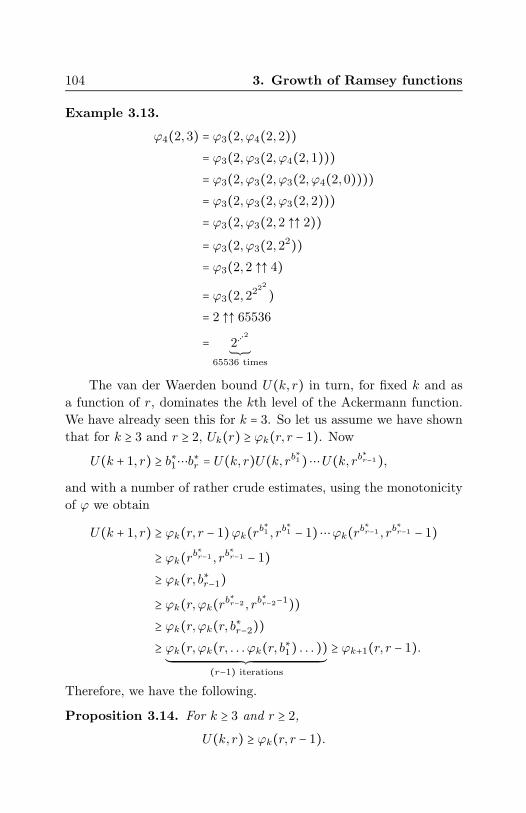
104 3. Growth of Ramsey functions
Example 3.13.
ϕ4(2, 3) = ϕ3(2, ϕ4(2, 2))= ϕ3(2, ϕ3(2, ϕ4(2, 1)))= ϕ3(2, ϕ3(2, ϕ3(2, ϕ4(2, 0))))= ϕ3(2, ϕ3(2, ϕ3(2, 2)))= ϕ3(2, ϕ3(2, 2 ↑↑ 2))= ϕ3(2, ϕ3(2, 22))= ϕ3(2, 2 ↑↑ 4)
= ϕ3(2, 2222
)= 2 ↑↑ 65536
= 2⋰2
T65536 times
The van der Waerden bound U(k, r) in turn, for fixed k and as
a function of r, dominates the kth level of the Ackermann function.
We have already seen this for k = 3. So let us assume we have shown
that for k ≥ 3 and r ≥ 2, Uk(r) ≥ ϕk(r, r − 1). Now
U(k + 1, r) ≥ b∗1⋯b∗r = U(k, r)U(k, rb∗1) ⋯U(k, rb
∗r−1),
and with a number of rather crude estimates, using the monotonicity
of ϕ we obtain
U(k + 1, r) ≥ ϕk(r, r − 1)ϕk(rb∗1 , rb
∗1 − 1) ⋯ϕk(rb
∗r−1 , rb
∗r−1 − 1)
≥ ϕk(rb∗r−1 , rb
∗r−1 − 1)
≥ ϕk(r, b∗r−1)
≥ ϕk(r,ϕk(rb∗r−2 , rb
∗r−2−1))
≥ ϕk(r,ϕk(r, b∗r−2))≥ ϕk(r,ϕk(r, . . . ϕk(r, b∗1) . . . ))
UVVVVVVVVVVVVVVVVVVVVVVVVVVVVVVVVVVVVVVVVVVVVVVVVVVVVVVVVVVVVVVVVVVVVVVVVVVVVVVVVVVVVVVVVVVVVWVVVVVVVVVVVVVVVVVVVVVVVVVVVVVVVVVVVVVVVVVVVVVVVVVVVVVVVVVVVVVVVVVVVVVVVVVVVVVVVVVVVVVVVVVVVX(r−1) iterations
≥ ϕk+1(r, r − 1).
Therefore, we have the following.
Proposition 3.14. For k ≥ 3 and r ≥ 2,
U(k, r) ≥ ϕk(r, r − 1).

3.3. Hierarchies of growth 105
While, as we have seen, the growth of ϕk(r, r) is already rather
impressive for k ≥ 4, truly “explosive” growth is generated when we
allow k to vary, too.
Exercise 3.15. Show that Uω(k) = U(k, k) eventually dominates
ϕm(k, k) for any m.
3.3. Hierarchies of growth
In the previous section we introduced the Ackermann function ϕ. We
saw that the associated level functions, ϕk, track the growth of the
kth van der Waerden bound Uk(r). In this section we will connect
these functions to important concepts from computability theory, the
notion of a primitive recursive function and the Grzegorczyk hier-
archy. We will also see how we can generate even faster-growing
functions, by extending the construction into the transfinite. This is
where ordinals will be needed again.
Primitive recursive functions. When we introduced the Acker-
mann function ϕ (Definition 3.10), we observed that each level ϕk
is obtained by iterating the previous one—multiplication iterates ad-
dition, exponentiation iterates multiplication, and so on. We also
defined an upper bound U(k, r) for the van der Waerden number
W (k, r) using a similar iteration. The actual definition of U(k, r)was a bit more complicated than that of ϕ, but essentially we used
two basic operations to define U(k, r):
Composition: Given functions h(x1, . . . , xm) and
g1(x1, . . . , xn), . . . , gm(x1, . . . , xn), we can compose these
functions to define a new function
f(x1, . . . , xm) = h(g1(x1, . . . , xn), . . . , gm(x1, . . . , xn)).
Recursion: Given functions g(x1, . . . , xn) and h(x1, . . . , xn, y, z),we can define f by recursion from g and h as
f(x1, . . . , xn, 0) = g(x1, . . . , xn),f(x1, . . . , xn, y + 1) = h(x1, . . . , xn, y, f(x1, . . . , xn, y)).
The arities of the functions considered here are arbitrary but have to
be finite.

106 3. Growth of Ramsey functions
Each function ϕk, as well as each kth level of the van der Waerden
bound Uk, can be obtained by a finite number of applications of these
two operations to a set of basic functions: x+ y in the case of ϕ, r+1
(the value of W (2, r)), multiplication, exponentiation, and integer
division for U .
Functions that can be obtained this way belong to an important
family of functions—the primitive recursive functions. To define them
for all finite arities, we introduce the following basic functions.
Zero function: Zero(x) = 0.
The successor function: S(x) = x + 1.
The projection functions: P in(x1, . . . , xn) = xi.
Definition 3.16. The family of primitive recursive functions is
the smallest family of functions f ∶ Nn → N (where n ∈ N can be
arbitrary) that contains the three basic functions and is closed under
composition and recursion.
In other words, a function is primitive recursive if it can be ob-
tained from the basic functions by a finite number of applications
of composition and recursion. For example, addition + is primitive
recursive as it can be defined as follows:
x + 0 = P 11 (x),
x + (y + 1) = S(P 13 (x, y,+(x, y))).
One can continue inductively and obtain the following.
Proposition 3.17. Every level ϕk(x, y) of the Ackermann function
is primitive recursive.
The family of primitive recursive functions includes many more
functions. For example, the common functions of elementary num-
ber theory, such as gcd and remainder, are primitive recursive. The
verification of this is often a little tedious. One has to build up a
“library” of primitive recursive functions. We give some examples.
Lemma 3.18. The predecessor function
x Y 1 =⎧⎪⎪⎨⎪⎪⎩
x − 1 if x > 0,
0 if x = 0
is primitive recursive.

3.3. Hierarchies of growth 107
Proof. We can define this recursively as
0 Y 1 = 0 = Zero(0),(x + 1) Y 1 = x = (x Y 1) + 1 = S(x Y 1).
�
Exercise 3.19. Show that the following functions are primitive re-
cursive:
x Y y, max(x, y), min(x, y), ∣x − y∣.
An important property of the primitive recursive functions is their
closure under bounded search procedures.
Definition 3.20. Given a predicate P (x, y) on Nn+1, the bounded
μ-operator applied to a predicate P (x, y) is defined as
μz < y [P (x, z)] =⎧⎪⎪⎪⎪⎨⎪⎪⎪⎪⎩
z if z is the least natural number < y
such that P (x, y) holds
,
y if no such z exists.
This means that the bounded μ-operator applied to a predicate re-
turns the least witness less than y such that the predicate holds.
Proposition 3.21. If g(x, y) is primitive recursive, then so is
f(x, y) = μz < y [g(x, z) = 0].
For a proof see, for example, [54, Section 6.1].
Exercise 3.22. Use the closure under the bounded μ-operator to
show that the following functions are primitive recursive:
div(x, y) = result of integer division of x by y,
rem(x, y) = remainder of integer division of x by y.
In the late 19th century, work by Dedekind [11] and Peano [48,
49] demonstrated that definitions by induction play an important role
in the development of number theory from first principles (axioms),
and that any axiomatic framework for number theory must include a
principle ensuring that functions described by induction (recursion)
are indeed well-defined. This led to the introduction of the family

108 3. Growth of Ramsey functions
of primitive recursive functions as the closure of the basic arithmetic
functions under composition and inductive definitions.
Furthermore, every primitive recursive function is computable (in
an intuitive sense), as we can compute any value using a finite de-
terministic procedure, unraveling the recursion, as we did in Exam-
ple 3.13. Moreover, all the usual number-theoretic functions, which
are intuitively computable, can also be shown to be primitive recur-
sive.
The Grzegorczyk hierachy. The Ackermann function provided the
first example of a computable function (in the intuitive as well as in
a formal sense) that was not primitive recursive. The key here is
that the diagonal Ackermann function eventually dominates every
primitive recursive function. In fact, the levels ϕk of the Ackermann
function form a kind of “spine” of the primitive recursive functions,
in terms of their growth behavior. To formulate this, it will be useful
to have a unary version of the Ackermann level functions.
Definition 3.23. The family of functions {Φn∶n ∈ N} is defined by
Φn(x) =⎧⎪⎪⎨⎪⎪⎩
2 if n = 0,
ϕn(2, x) if n > 0.
Hence we have
Φ0(x) = x + 2,
Φ1(x) = 2x,
Φ2(x) = 2x,
Φ3(x) = 2 ↑↑ (x + 1),
and in general, for n ≥ 1,
Φn+1(0) = 2,
Φn+1(x + 1) = Φn(Φn+1(x)).
In other words, Φn+1 is obtained by iterating Φn. If we denote the
n-iteration of a function f by f (n), then
Φn+1(x) = Φ(x)n (2).

3.3. Hierarchies of growth 109
We already observed that by iterating a function we are able to
generate another function that grows much faster than the original
function. This can be made precise by defining a hierarchy on the
family of primitive recursive functions that categorizes them accord-
ing to their growth behavior. Such a hierarchy was introduced by
Grzegorczyk [28] and has since become known as the Grzegorczyk
hierarchy
E0 ⊂ E1 ⊂ E2 ⊂ ⋯.
E0 is the smallest family of functions containing the base functions
Zero, x + y (instead of successor), and P in and that is closed under
composition and limited recursion with respect to E0. Here limited
recursion means that if f is defined via recursion from g, h ∈ E0 and
there exists a function j ∈ E0 such that for all x1, . . . , xn, y ∈ N,
f(x1, . . . , xn, y) ≤ j(x1, . . . , xn, y),
then f ∈ E0. In other words, to add a function to E0, the growth of
the function has to be bounded by a witness j already known to be
in E0.
Once En is defined, En+1 is defined as the smallest family of func-
tions containing all functions from En, the function Φn (or rather,
a slight variant thereof) and which is closed under composition and
limited recursion.
Defining En via a closure property ensures that each En is very
robust with respect to operations of its own type. For example, E2
contains the multiplication function, and if we multiply two functions
from E2, we obtain a function in E2 again. On the other hand, if
we iterate a function from En, we obtain a function in En+1. More
generally, if g, h ∈ En and f is defined from g and h via recursion, then
f ∈ En+1. Moreover, for all n, Φn ∈ En+1 ∖ En. In other words, the
hierarchy is proper.
The Grzegorczyk hierarchy captures all primitive recursive func-
tions with respect to their growth behavior in the following sense.
Theorem 3.24.
(a) Every primitive recursive function is contained in some En.

110 3. Growth of Ramsey functions
(b) If f is a unary function in En, then f is eventually domi-
nated by Φn.
It would go beyond the scope of this book to prove the theorem
here, so we refer to the book by Rose [56].
Corollary 3.25. The diagonal function Φω(x) = Φx(x) is not prim-
itive recursive.
Proof. If Φω were primitive recursive, there would exist k and x0
such that for all x > x0,
Φω(x) ≤ Φk(x).
But for x > max(k, x0), we have by the monotonicity of the Φn that
Φk(x) < Φx(x) = Φω(x),
which is a contradiction. �
Corollary 3.26. The Ackermann function ϕ(x, y, n) and the van der
Waerden upper bound U(k, r) are not primitive recursive.
A word of caution: You may be tempted to think now that if
a function is bounded by some Φn, it is primitive recursive. How-
ever, this is far from the truth. In Chapter 4, we will encounter a
{0, 1}-valued function that is not even (Turing) computable, let alone
primitive recursive.
Extending the hierarchy. The functions Φn and diagonal function
Φω(x) = Φx(x) give us a blueprint of how to construct ever faster-
growing functions.
We iterated Φn to create the faster-growing function Φn+1. Let
us apply this now to the diagonal function Φω:
Φω+1(0) = 2,
Φω+1(x + 1) = Φω(Φω+1(x)).
As you can probably tell, we have chosen the index ω with the idea
in mind that the ordinals will help us index our extended hierarchy

3.3. Hierarchies of growth 111
beyond the finite levels. So, in general, assume that we have defined
the function Φα(x) for some ordinal α, and let
Φα+1(0) = 2,
Φα+1(x + 1) = Φα(Φα+1(x)).
Note that even though the functions are indexed by ordinals, they are
still functions from N to N.
What this definition does not tell us is how to define Φα in the
case where α is a limit ordinal. For α = ω, we took the diagonal of
the functions “leading up to it”. We can do something similar for an
arbitrary limit ordinal α by putting
Φα(x) = Φαx(x),
where αx is a sequence of ordinals with limit α, i.e. sup{αx∶x ∈ N} = α.
Any such sequence is called a fundamental sequence for α.
There are two issues: First, this only works for limit ordinals with
cofinality ω (recall the definition of cofinality, Definition 2.43). As we
are only interested in Φα for countable α, this does not really present
a problem. Second, there are multiple ways to choose a fundamental
sequence. For example, if α = ω + ω, both
ω + 1, ω + 3, ω + 5, . . . and ω + 2, ω + 4, ω + 6, . . .
converge to α. Is there a canonical way of selecting a fundamental
sequence? If we consider only α < ε0 (recall that ε0 was the least
ordinal ε for which ωε = ε), there is indeed such a way, given through
the Cantor normal form.
Theorem 3.27 (Cantor normal form). Every ordinal 0 < α < ε0 can
be represented uniquely in the form
α = ωβ1 + ⋯ + ωβn ,
where n ≥ 1 and α > β1 ≥ ⋅ ⋅ ⋅ ≥ βn.
In fact, if we only require α ≥ β1, every ordinal α has a unique
representation of this form.
For example, α = ωω2+3 + ω2 + ω2 + 1 + 1 + 1 is in Cantor normal
form. (Recall that ω0 = 1.)

112 3. Growth of Ramsey functions
Proof. We proceed by induction. For α = 1, we have α = ω0. Suppose
now that the assertion holds for all β < α. Let
γ∗ = sup{γ∶ ωγ ≤ α}.
Then γ∗ is the largest ordinal such that ωγ∗ ≤ α, and as α < ε0, γ∗ < α.
Note that for any two ordinals δ ≤ α, there exists a unique ρ
such that α = δ + ρ. We simply let ρ be the order type of the set
{β∶ δ < β ≤ α}.Now let ρ be the unique ordinal such that α = ωγ∗ + ρ. By the
choice of γ∗, we must have ρ < α (see Exercise 3.28), and by the
inductive hypothesis, ρ has a normal form
ρ = ωγ1 + ⋯ + ωγk .
Then
α = ωγ∗ + ωγ1 + ⋯ + ωγk ,
with γ∗ ≥ γ1 ≥ ⋅ ⋅ ⋅ ≥ γk, as desired. �
Exercise 3.28. Show that ωγ + α = α implies ωγ+1 ≤ α.
Exercise 3.29. Use transfinite induction to show that the Cantor
normal form is unique.
How can we use the Cantor normal form in selecting a fundamen-
tal sequence for α?
Suppose we have
α = ωβ1 + ⋯ + ωβn ,
with β1 ≥ ⋅ ⋅ ⋅ ≥ βn. If α is a limit ordinal, we must have βn ≥ 1. If βn
is a successor ordinal, i.e. if βn = γ + 1, we can let
αk = ωβ1 + ⋯ + ωγ ⋅ k,
and so limk αk = α. If βn is a limit ordinal, we have βn < α (since
α < ε0), and we can construct a fundamental sequence by induc-
tion: Assume that we have constructed one for βn, say (γk)k∈N; then(αk)k∈N given by
αk = ωβ1 + ⋯ + ωβn−1 + ωγk
is a fundamental sequence for α.

3.4. The Hales-Jewett theorem 113
To make our definition of Φα rigorous (assuming α < ε0 is a
limit ordinal), let us write α[k] for the kth term in the canonical
fundamental sequence for α defined above. We put
Φα(x) = Φα[x](x).
Finally we define β1 = ω and βn+1 = ωβn , that is, βn is a tower of
n-many ω’s. Then let
Φε0(x) = Φβx(x).
The functions Φα, α ≤ ε0, are known as the Wainer hierarchy.
They are still functions from N to N. We can even write a computer
program to evaluate them. This seems strange at first sight, as the
ordinals used to index them are infinite. But they are defined via
recursion, and there are no infinite descending chains of ordinals.
Only finitely many steps of “unraveling” are required. Try to compute
Φω2+17(3), and you will get the idea. (Of course the running time of
this algorithm on any computer would exceed the expected life of this
computer by far.)
Still, the Φα, in particular Φε0 , seem somewhat unreal, a pure
construct based on the infinitude of ordinals. Are there any “real”
mathematical objects tied to this kind of growth?
The remaining two sections of this chapter will go in opposite
directions with respect to this question. First, we will bring the van
der Waerden numbers to level Φ4. After that, we will see that a rather
simple modification of Ramsey’s original theorem will produce a true
growth behavior at the level of ε0.
3.4. The Hales-Jewett theorem
While van der Waerden’s theorem proved the existence of patterns in
sequences of numbers, the theorem of Hales and Jewett [29], origi-
nally proven in 1963, deals with more general combinatorial geometric
objects.
The combinatorial cube Cnt is the set of n-tuples with entries
in [t] ∶= {1, . . . , t}; each n-tuple is called a combinatorial point. One
can picture this as an n-dimensional cubic array with side length t.
An r-coloring on a combinatorial cube is then a function c ∶ Cnt →

114 3. Growth of Ramsey functions
[r]. Each cell in the array is labeled with one of r colors. As an
example, consider the game tic-tac-toe. A standard tic-tac-toe board
is a representation of the combinatorial cube C23 , and a game of tic-
tac-toe is essentially taking turns defining a 2-coloring on the cube.
With the game of tic-tac-toe in mind, it makes sense to ask about
the existence of monochromatic lines.
Definition 3.30. For n, t > 1, a combinatorial line in Cnt is a
subset of t distinct combinatorial points L1, . . . , Lt where, for each
1 ≤ i ≤ n, either
Lτ,i = Lσ,i for all 1 ≤ τ, σ ≤ t,
that is, the ith coordinate is constant, or
Lτ,i = τ for all 1 ≤ τ ≤ t,
which means that the ith coordinate varies with τ .
Note that in a combinatorial line, at least one coordinate has to
vary with τ . An example of a combinatorial line in C45 is
L1 = (1 4 1 2),L2 = (2 4 2 2),L3 = (3 4 3 2),L4 = (4 4 4 2),L5 = (5 4 5 2).
The notion of a combinatorial line is slightly stricter than for instance
the lines allowed in tic-tac-toe, because the diagonal from the upper
left to the lower right corner on a tic-tac-toe board,
(1 3)(2 2)(3 1),
is not a combinatorial line, while the lower left to upper right diagonal
(1 1)(2 2)(3 3)
is.
Exercise 3.31. Determine all combinatorial lines for C24 . How many
are there?

3.4. The Hales-Jewett theorem 115
We will often use an alternative notation for combinatorial lines.
A (t, n)-∗-word is a sequence over {1, . . . , t}∪{∗} of length n where at
least one entry is a ∗. Any (t, n)-∗-word L represents a combinatorial
line in Cnt by simultaneously substituting τ for every occurrence of ∗
in L, for 1 ≤ τ ≤ t. We denote the resulting point in Cnt by L(τ). The
first example above corresponds to the ∗-word L = (∗ 4 ∗ 2), whilethe diagonal on a tic-tac-toe board is given by (∗ ∗).
Exercise 3.32. Represent the combinatorial lines in C24 using ∗-
words. Derive a general formula for the number of combinatorial
lines in Cnt .
Theorem 3.33 (Hales and Jewett). For any integers t, r > 1, there
exists an integer HJ (t, r) such that for any n ≥ HJ (t, r), every r-
coloring of Cnt has a monochromatic combinatorial line.
The integers HJ (r, t) are called the Hales-Jewett numbers.
It is well known that the standard tic-tac-toe is a boring game; with
optimal strategies, the game will always end in a tie. This means that
there exist (lots of) 2-colorings of C23 which contain no monochromatic
combinatorial lines, and therefore HJ (3, 2) > 2. In 2014, Hindman
and Tressler [33] proved that HJ (3, 2) = 4. We should probably play
tic-tac-toe in four-dimensions.
The rather geometric concept of combinatorial lines is very ver-
satile. Many combinatorial statements can be transformed into an
equivalent statement about combinatorial lines. This makes the Hales-
Jewett theorem extremely powerful. We illustrate this by deriving van
der Waerden’s theorem from it.
Proposition 3.34. If HJ (t, r) exists, then W (t, r) exists and it holds
that W (t, r) ≤ tHJ(t,r), where W (t, r) is the van der Waerden number
(defined in Theorem 3.3).
Proof. Consider the integers from {0, . . . , tn − 1} in their base-t rep-
resentation:
x = x0 + x1t + ⋯ + xntn−1,
where 0 ≤ xi ≤ t − 1. We can identify x with (x0, x1, . . . , xn), and this
provides a bijection p ∶ {0, . . . , tn−1} → Cnt . (Note that we are slightly

116 3. Growth of Ramsey functions
deviating from our previous notation by having the coordinates range
from 0 to t − 1 rather than from 1 to t.) Then, any r-coloring on
[0, tn − 1] induces an r coloring on Cnt .
If we assume that the Hales-Jewett theorem is true and that n >HJ (t, r), then Cn
t has a monochromatic line, say L. Let A be the
subset of {0, . . . , n−1} for which the entries of L are a ∗ and let B be
{0, . . . , n − 1} ∖ A. Then the preimage in {0, . . . , tn − 1} of any point
on the line L is of the form
x = p−1(L(τ)) =n
∑i=1
L(τ)i ti−1 = ∑i∈A
τti−1 + ∑i∈B
Liti−1.
If we let D = ∑i∈A ti−1 and C = ∑i∈B Liti−1, then x = Dτ + C, and
therefore the preimage of L forms a monochromatic arithmetic pro-
gression in {0, . . . , tn−1} of length t. �
Exercise 3.35. Determine the arithmetic progression in N induced
by L = (∗ 3 ∗) in C34 .
The original proof by Hales and Jewett used a double induc-
tion and hence gave bounds that, similar to van der Waerden’s the-
orem, grow in an Ackermann-like fashion. In 1988, Shelah [58] gave
a completely new proof that brought the growth of the Hales-Jewett
numbers (and hence, by Proposition 3.34, also the Van der Waerden
numbers) “down to Earth”, by establishing the existence of HJ (t, r)as a single induction on t (with r arbitrary but fixed).
The proof of the Hale-Jewett theorem given here follows the one
by Shelah, where we adopt some of the organizational structure (and
notation) from the presentation of [24].
Shelah was able to reduce the problem for r-colorings of Cnt to r-
colorings of Cnt−1. In fact, if the given coloring is not able to distinguish
between t − 1 and t, we can extend a monochromatic line of length
t − 1 to one of length t.
To be specific, two points x = (x1, . . . , xn) and y = (y1, . . . , yn) in
Cnt are t-close if for all i ≤ n,
(a) xi < t − 1 if and only if yi < t − 1, and
(b) xi < t − 1 implies xi = yi.

3.4. The Hales-Jewett theorem 117
In other words, x and y agree on entries below t− 1 and can differ by
at most 1 on the other entries. For example,
(1 2 4 4 1 3) and (1 2 3 4 1 4)are 4-close points in C6
4 , whereas
(1 2 4 2 1 3) and (4 2 3 4 1 4)are not.
An r-coloring c on Cnt is t-blind if any pair of t-close points has
the same color.
Lemma 3.36. If HJ (t−1, r) exists, n ≥ HJ (t−1, r), and c is a t-blind
r-coloring on Cnt , then there exists a monochromatic line.
Proof. Restrict c to a coloring on Cnt−1 ⊂ Cn
t . By assumption, there
is a monochromatic line L in Cnt−1. This line is a set of t − 1 points
and is a subset of a unique line L+ in Cnt having one additional point
which is equal to L(t). We have the following:
(a) c(L(1)) = c(L(2)) = ⋯ = c(L(t−1)), because L is monochro-
matic in Cnt−1;
(b) c(L(t − 1)) = c(L(t)), because L(t − 1) and L(t) are t-close
and the coloring is t-blind.
Therefore, the entire line L is monochromatic in Cnt . �
Of course not every coloring of Cnt is t-blind. But Shelah managed
to show that for any coloring on a sufficiently large cube, there is a
subset of a combinatorial substructure where the coloring is t-blind.
In the following, if a coloring restricted to a combinatorial structure
is t-blind, we will call this structure t-blind, too. For example, we will
speak of blind combinatorial lines.
Shelah’s combinatorial substructures are built from rather simple
blocks. For 1 ≤ a ≤ b ≤ n, define a Shelah line2 La,b in Cnt as the
∗-word of the form
(t − 1 ⋯ t − 1UVVVVVVVVVVVVVVVVVVVVVVVVVVVWVVVVVVVVVVVVVVVVVVVVVVVVVVX(a − 1)-many
∗ ⋯ ∗^
(b − a + 1)-many
t ⋯ tO
(n − b)-many
)
2The naming of these combinatorial structures after Shelah is due to Graham,Rothschild, and Spencer [24], and we follow them here.

118 3. Growth of Ramsey functions
In C64 , the Shelah line L3,5 is the ∗-word (3 3 ∗ ∗ ∗ 4), which
induces the line
(3 3 1 1 1 4),(3 3 2 2 2 4),(3 3 3 3 3 4),(3 3 4 4 4 4).
Let us call a point on a Shelah line a Shelah point. Such a point
depends only on a, b, and the value τ of ∗. Therefore, there are no
more than t ⋅ n2 Shelah points in Cnt .
3
Lemma 3.37 (Shelah line pigeonhole principle). If n ≥ r, then for
any r-coloring c of Cnt , there exists a Shelah line restricted to which
c is t-blind.
Proof. For 0 ≤ i ≤ n, let Pi ∈ Cnt be the point where the first i
coordinates are equal to t − 1 and the last n − i coordinates are equal
to t. There are n+1 such points, and each has been colored with one
of r colors, so by the pigeonhole principle, at least two such points
have the same color, say Pi and Pj . Note that these are both Shelah
points on the same line with Pj = Li+1,j(t − 1) and Pi = Li+1,j(t), soc(Li+1,j(t − 1)) = c(Li+1,j(t)) and therefore the Shelah line Li+1,j is
t-blind. �
A single Shelah line will not be enough for our purposes; we need
the simultaneous existence of multiple Shelah lines.
A combinatorial s-space, Σs, is the concatenation of s combi-
natorial lines of variable dimensions over the same alphabet. We can
represent the space as the set of s-tuples whose entries are points on
combinatorial lines,
(L1(τ1), L2(τ2), . . . , Ls(τs)).
Each Li is a combinatorial line in Cnit for some ni, and each τi can
vary independently. The combinatorial s-space Σs can be realized as
a subset of Cnt where n = ∑ni.
3This bound is clearly not optimal, but it facilitates counting later while havinglittle impact on the overall growth estimate.

3.4. The Hales-Jewett theorem 119
A Shelah s-space is a combinatorial space whose coordinates are
all Shelah lines. A Shelah line has one degree of freedom (the value
of the ∗-block), so there is a canonical bijection between a Shelah
s-space S and Cst . Let us denote this bijection by π ∶ Cs
t → S. For
example, consider the Shelah 3-space
(2 2 ∗ 3) × (2 ∗) × (2 ∗ ∗ ∗ 3 3).
While points in this space live in C123 , any such point is completely
determined by the respective values of ∗ in the three Shelah lines.
Therefore, there is a canonical bijection between the space and C33 .
Given a coloring c of a Shelah s-space, we call c t-blind if the
induced coloring c∗ = c ○ π is t-blind.
Lemma 3.38 (Existence of blind Shelah spaces). Given integers
r, s, t ≥ 1, there exists an N such that every r-coloring of CNt con-
tains a Shelah s-space on which the coloring is t-blind.
Proof. Suppose a sufficiently large N is given and we want to find a
partition
N = N1 + ⋯ + Ns
such that there exists a blind Shelah space the lines of which lie in
CNit . We can define the Ni and the corresponding Shelah lines via
reverse induction: Starting with Ns, at each step i we determine how
large to choose Ni in relation to the precedingNj , j < i, so that we can
not only find a t-blind Shelah line in CNit but also leave enough points
in the preceding CNj
t color compatible with the Shelah line in CNit .
The main tool for this will be an iterated application of Lemma 3.37,
the Shelah line pigeonhole principle.
Let us assume N = N1 + ⋯ + Ns and thus
(CN1t , . . . , CNs
t ) ≅ CNt .
Given a coloring c on CNt , we define an equivalence relation on CNs
t
as follows: For two points y, y∗ ∈ CNst , we will say that y and y∗ are
equivalent if for all Shelah points xi in CNit with i < s,
c(x1, . . . , xs−1, y) = c(x1, . . . , xs−1, y∗).

120 3. Growth of Ramsey functions
Two points are hence equivalent if they have identical coloring be-
havior with respect to all (s−1)-combinations of Shelah point prede-
cessors.
Since each CNit has no more than tN2
i Shelah points, each point
in CNst has at most
ts−1s−1
∏j=1
N2j =∶ Ms
such Shelah (s−1)-predecessors. Moreover, each of these Shelah (s−1)-predecessors is colored one of r ways, so each point y ∈ CNs has
rMs possible coloring behaviors with respect to its Shelah (s − 1)-predecessors. Therefore, there are at most rMs equivalence classes.4
Equivalence relations naturally correspond to colorings (by as-
signing each equivalence class a different color). Our equivalence re-
lation thus defines an rMs-coloring on CNst . If we require Ns ≥ rMs ,
we can apply the Shelah line pigeonhole principle (Lemma 3.37) and
conclude that CNst contains a t-blind Shelah line with respect to this
new coloring, that is, a line Ls in CNst where the points Ls(t−1) and
Ls(t) are in the same equivalence class.
Now that we have found a t-blind Shelah line in CNst , we will work
inductively backward to complete our t-blind Shelah space, while at
the same time bounding the Nj in terms of their predecessors (and
their predecessors only). Assume that we have found t-blind Shelah
lines Li+1, . . . , Ls in the last s − i cubes CNi+1t , . . . , CNs
t .
We define an equivalence relation on CNit similar to the one on
CNst : Two points y, y∗ ∈ CNi
t are equivalent if
c(x1, . . . , xi−1, y, zi+1, . . . , zs) = c(x1, . . . , xi−1, y∗, zi+1, . . . , zs)
for all Shelah points xj ∈ CNj
t , j < i, and all points zk ∈ Lk, k > i.
That is, the colorings agree with respect to all Shelah points in the
preceding components and all points chosen from the Shelah lines
already fixed in the subsequent components.
There are fewer equivalence classes now, though, because while
we can choose any Shelah point from CN1t through CNi−1
t , we have
4This is similar to the block-coloring patterns in the proof of van der Waerden’stheorem.

3.4. The Hales-Jewett theorem 121
restricted ourselves to only one of t Shelah points from CNi+1t through
CNst . Therefore, there are at most
i−1
∏j=1
(tN2j ) ⋅ ts−i = ts−1
i−1
∏j=1
N2j =∶ Mi
possible choices for the xj and zk. As before, this means that there
are rMi equivalence classes. We require Ni ≥ rMi , and as before the
Shelah line pigeonhole principle implies that CNj
t contains a t-blind
Shelah line, Li, with respect to this equivalence relation.
Continuing in this way, we obtain Shelah lines L1, . . . , Ls and
claim that the original coloring c is t-blind for the corresponding She-
lah s-space S.
It suffices to verify the following: If (z1, . . . , zi−1, y, zi+1, . . . , zs)and (z1, . . . , zi−1, y∗, zi+1, . . . , zs) are two points in S with y = t − 1
and y∗ = t, then the points have the same color.
By construction,
(x1, . . . , xi−1, y, zi+1, . . . , zs) and (x1, . . . , xi−1, y∗, zi+1, . . . , zs)
have the same color for any Shelah points x1 ∈ CN1t , . . ., xi−1 ∈ CNi−1
t .
But since each zj , j < i, is on the Shelah line Lj , the zj are clearly
Shelah points, from which the claim follows immediately.
Therefore, if we set the Ni as required in the construction,
(3.7)
N1 ∶= rts−1
,
Mi ∶= ts−1i−1
∏j=1
N2j and Ni ∶= rMi (1 < i ≤ s),
N ∶=s
∑i=1
Ni,
the existence of the constructed Shelah space is ensured and the
lemma is proved. �
The Hales-Jewett theorem can be deduced rather easily now.
Proof of the Hales-Jewett theorem. For any fixed r, we know
that HJ (1, r) = 1. Now assume that s ∶= HJ (t− 1, r) exists and let N
be defined as in the statement of Lemma 3.38. Let c be an r-coloring

122 3. Growth of Ramsey functions
of CNt . Lemma 3.38 guarantees the existence of a Shelah s-space
Σs = (L1, . . . , Ls) on which c is t-blind.
As before, we let π ∶ Cst → Σs be the canonical bijection between
Cst and Σs. We can pull back c to a coloring c∗ on Cs
t by letting
c∗ = π ○ c. By choice of s and Lemma 3.36, Cst has a monochromatic
line. The image of this line under π is a monochromatic line in Σs,
which is in CNt . �
As indicated earlier, Shelah’s proof gives a primitive recursive
bound on HJ(t, r) (and hence also on W (k, r)).
Corollary 3.39. For every r ≥ 1, HJ (t, r) (as a function of t) is
eventually dominated by Φ5(t).
Proof. Let S(t) be the function defined in the proof of Lemma 3.38,
that is, let S(1) = 1. For s = S(t − 1), let S(t) = N , where N is as
in the last line of (3.7). Inspecting the definition of S, we see that
from some point on, S(t) is significantly larger than both r and t. In
particular, with s = S(t − 1) we have
N1 = rts−1
≤ sss
≤ Φ3(s)and
Mi = ts−1i−1
∏j=1
N2j ≤ (Ni−1)3s,
and thus, for sufficiently large t (and hence sufficiently large s),
Ni ≤ r(Ni−1)3s ≤ 222Ni−1
.
Every iteration of Ni adds three more exponents to an exponential
tower (the ↑↑ function), and hence adds 3 to an argument of Φ3.
Therefore,
Ns ≤ Φ3(s + 3(s − 1)) ≤ Φ3(4s),and
S(t) = N = N1 + ⋯ + Ns ≤ 2Ns ≤ Φ3(4s + 1).A direct calculation shows that S(3) ≤ Φ4(8). So if we assume, in-
ductively, that S(t − 1) ≤ Φ4(2t), thenS(t) ≤ Φ3(4s + 1) = Φ3(4S(t − 1) + 1)
≤ Φ3(4Φ4(2t) + 1) ≤ Φ3(Φ4(2t + 1)) = Φ4(2(t + 1)).

3.5. A really fast-growing Ramsey function 123
Therefore S(t) is eventually dominated by a function that is a com-
bination of two functions from E5 and therefore, by Theorem 3.24, is
eventually dominated by Φ5. �
Of course, better bounds can be extracted from Shelah’s proof,
but here we were interested only in giving an explicit bound, as sim-
ply as possible, in terms of the Grzegorczyk hierarchy. By Proposi-
tion 3.34, the van der Waerden bound W (k, r) is also in E5.
3.5. A really fast-growing Ramsey function
Using a seemingly small tweak to Ramsey’s theorem, one can en-
sure that the corresponding Ramsey numbers grow faster than any
primitive recursive function. This was shown by Paris and Harring-
ton [47] and forms an integral part of their metamathematical anal-
ysis of Ramsey-type theorems, which we will describe in Chapter 4.
Let us call a set Y ⊆ N relatively large if
∣Y ∣ > minY.
Theorem 3.40 (Fast Ramsey theorem [47]). For all integers m,p, r ≥1, there exists N ∈ N such that whenever [N]p is r-colored, there exists
a relatively large, homogeneous subset Y ⊆ [N] of size at least m.
The only difference from the usual finite Ramsey theorem (The-
orem 1.31) is that the homogeneous set Y is required to be relatively
large. Given m,p, and r, we denote by PH (m,p, r) the least N with
the property asserted in the statement of the theorem.
Proof. The proof is a simple application of the compactness princi-
ple. We follow the blueprint given in Section 2.2.
Suppose that for some m, p, and r, there is no N which satisfies
the statement of the theorem. For each natural number n, let
Tn = {f ∶ [n]p → r such that there is
no homogeneous Y which is relatively large}.
This set is finite for all n. Moreover, for each f ∈ Tn+1 there is a unique
g ∈ Tn such that f is an extension of g, that is, g ⊂ f . Therefore, we

124 3. Growth of Ramsey functions
have that the partially ordered set
T ∶= ⋃Tn
is a finitely branching tree which, by the assumption that Tn is non-
empty for all n, is infinite.
By Konig’s lemma (Theorem 2.6), we have an infinite path
f1 ⊂ f2 ⊂ ⋯
in T with each fi ∈ Ti. Let f = ⋃ fi, which is an r-coloring of the
natural numbers. By the infinite Ramsey theorem (Theorem 2.1),
there exists an infinite, homogeneous X ⊂ N, say
{x1 < x2 < x3 < ⋯}.
If we now restrict this set to the first s ∶= x1 + 1 elements
{x1, x2, . . . , xs},
the set is a homogeneous subset of [xs] which is relatively large. This
is a contradiction. �
We will show that PH grows very fast. To facilitate the analy-
sis, we introduce a slight variant of the function family {Φn∶n ∈ N}.Define functions Ψn by
Ψ0(x) = x + 1,
Ψn+1(x) = Ψ(x)n (x).
Compare this with Definition 3.23.
Exercise 3.41. Show that Ψ1(x) = 2x and Ψ2(x) = x ⋅ 2x.
The functions Ψn have a growth behavior similar to the Φn. In
fact, each Ψn appears at the same level of the Grzegorczyk hierarchy
{En∶n ∈ N} as Φn.
Theorem 3.42. For every n ≥ 1, PH (n + 2, 2, n + 1) ≥ Ψn(n + 1).
Proof. We define a 2-coloring c1 as follows: Split the set [2,∞) into
intervals [x, 2x), i.e.
[2, 4) ∪ [4, 8) ∪ [8, 16) ∪ ⋯.

3.5. A really fast-growing Ramsey function 125
Call these intervals the type 1 blocks. If i and j lie in the same type 1
subset, put c(i, j) = 1. Otherwise, let c1(x, y) = 0.
If A is a homogeneous subset of color 1, then A ⊂ [x, 2x) for
some x, which means that ∣A∣ ≤ x and hence A is not relatively large.
Therefore, any relatively large, homogeneous subset Amust have color
0, and if ∣A∣ ≥ 3, then A has to contain at most one element each from
[2, 4) and [4, 8). Therefore, PH (3, 2, 2) ≥ 4 = Ψ1(2).Next, we define a type 2 block structure in a similar way. Split
[2,∞) into sets [x, x ⋅ 2x) (note that Ψ2(x) = x ⋅ 2x):
[2, 8) ∪ [8, 8 ⋅ 28) ∪ ⋯.
We keep the c1 color if c1(x, y) = 1. Additionally, we color the set
{i, j} with color 2 if i and j are in the same type 2 block but not the
same type 1 block.
Suppose A is a relatively large, homogeneous set. We argue as
before that the color of A cannot be 1. If it is 2, A must be a subset of
some interval [x, x ⋅2x). This interval is split into type 1 subintervals,
[x, 2x) ∪ [2x, 4x) ∪ ⋯ ∪ [x ⋅ 2x−1, x ⋅ 2x).
As we see, there are (x−1) such subintervals, and A contains at most
one element from each of these type 1 blocks (otherwise there would
be a pair of color 1). Therefore, ∣A∣ ≤ x holds in this case, too. It
follows that any relatively large, homogeneous subset of cardinality
greater than or equal to 4 must have at most one element from each
of
[2,Ψ2(2)), [Ψ2(2),Ψ2(Ψ2(2))), [Ψ(2)2 (2),Ψ(3)2 (2)),
and therefore
PH (4, 2, 3) ≥ Ψ(2)2 (2) ≥ Ψ2(3).
We can now continue inductively. The type n + 1 blocks have the
form [x,Ψn+1(x)) (where x itself is of the form Ψ(k)(3)), and to
define coloring cn+1 we keep cn except that we color {i, j} with color
n+ 1 if both i and j lie in the same type s+ 1 block but not the same
type s block.

126 3. Growth of Ramsey functions
By the definition of Ψn+1,
[x,Ψn+1(x)) = [x,Ψ(x+1)n (x))
= [x,Ψn(x)) ∪ ⋯ ∪ [Ψ(x)n (x),Ψ(x+1)n (x))UVVVVVVVVVVVVVVVVVVVVVVVVVVVVVVVVVVVVVVVVVVVVVVVVVVVVVVVVVVVVVVVVVVVVVVVVVVVVVVVVVVVVVVVVVVVVVVVVVVVVVVVVVVVVVVVVVVVVVVVVVVVVVVVVVVVVVVVVVVWVVVVVVVVVVVVVVVVVVVVVVVVVVVVVVVVVVVVVVVVVVVVVVVVVVVVVVVVVVVVVVVVVVVVVVVVVVVVVVVVVVVVVVVVVVVVVVVVVVVVVVVVVVVVVVVVVVVVVVVVVVVVVVVVVVVVVVVVVX
(x − 1) intervals
.
An argument similar to the one in the n = 2 case then yields
PH (n + 3, 2, n + 2) ≥ Ψn+1(n + 2),
which, by way of induction, proves the theorem. �
Corollary 3.43. The function f(x) = PH (x + 3, 2, x + 1) eventually
dominates Ψn, for all n, and therefore also every primitive recursive
function.
One can continue along these lines for higher values of p (that is,
look at p-sets instead of just pairs). The analysis becomes much more
involved. In a landmark paper, Ketonen and Solovay [40] were able
to show that
PH (x + 1, 3, x) eventually dominates every Φα(x) with α < ωω,
PH (x + 1, 4, x) eventually dominates every Φα(x) with α < ωωω
,
⋮
The diagonal function PH(x + 1, x, x) will then eventually dominate
every function Φα(x) with α < ε0.
Ketonen and Solovay’s argument is an elementary combinatorial
analysis, but rather complicated and long, and we will not reproduce
it here. We hope nevertheless to have conveyed some of the explo-
sive growth that is produced by requiring homogeneous sets to be
relatively large. The basic idea is that certain colorings can force a
relatively large homogeneous set to have rather large gaps. This is a
phenomenon we will encounter again.
On its own, the results of this section might appear to be a mere
mathematical curiosity—a slight variation on Ramsey’s theorem caus-
ing explosive growth of the accordant Ramsey numbers. Their sig-
nificance lies in the ties to the metamathematics of arithmetic, and

3.5. A really fast-growing Ramsey function 127
to the seminal developments in this area in the 20th century, most
notably Godel’s incompleteness theorems. It takes a bit of work to
develop the necessary background for this, and we will embark on it
in the next chapter.


Chapter 4
Metamathematics
4.1. Proof and truth
When do we consider a mathematical proposition to be true?
The longer one thinks about it, the more delicate this question
may become.
Some statements seem to be so obvious that their truth is self-
evident, such as the fact that there is no greatest natural number.
For other statements, less obvious ones, we require a proof to con-
vince ourselves. As an example, take the proposition that there is no
greatest prime number.
But what if we cannot find a proof, nor are we able to disprove
the assertion? The famous open mathematical problems come to
mind. Consider the Goldbach conjecture, for example, which states
that every even integer greater than 2 can be written as the sum of
two primes. This is a perfectly reasonable mathematical statement,
and probably most mathematicians would say that the conjecture
either holds or fails, but we just do not know yet which is the case.
When light is finally shed on the Goldbach conjecture, it will be in
the form of a proof of either the statement
∀m ∈ Z (m > 2 and m even ⇒ ∃p1, p2 prime (p1 + p2 = m))
or its negation
∃m ∈ Z (m > 2 and m even and ∀p1, p2 prime (p1 + p2 ≠ m)).
129

130 4. Metamathematics
Note that to prove the negation, all we have to do is exhibit a single
even number m and check for all pairs of prime numbers smaller than
m that they do not sum to m. It is a simple task that a computer
could do. And mathematicians have been using computers to search
for such an m, but so far, they have not found one.1
But why should we assume that a proof will in fact be found?
Could it even be that no proof exists? What would that even mean?
It is a remarkable achievement of mathematical logic to not only
rigorously define what constitutes a mathematical proof (in other
words, proofs are established as mathematical objects, the same way
that continuous functions are mathematical objects) but also show
that there are statements which, in a certain well-defined sense, can-
not be settled by proof at all, that is, neither the statement nor its
negation is provable.
What exactly constitutes a proof? We have already given plenty
of proofs in this book, and if we try to extract the essential features
common to all of them, we might come up with the following list:
● A proof derives the statement we want to prove from other
statements, either statements we have proved before, or ba-
sic assumptions we make about the objects we are dealing
with (usually referred to as “axioms”).
● The derivation consists of finitely many steps. In each step
we advance the argument by applying a logical rule, such as
if A implies B and A holds, then B holds.
● Each step should be so simple that everyone, even a com-
puter, can check its validity.
● If we prove something, it should of course be true.
While the first point is hopefully acceptable, the other three are more
problematic. Are proofs really finite? Of course, no one would be
able to read a proof of infinite length, but don’t we sometimes have
to check infinitely many cases? We do not check them all in the end,
but usually do one case and then argue something like “the other
cases are similar”. Furthermore, not every step in a proof seems to
1At the time this book was written, all numbers up to 4×10¹⁷ have been checked.

4.1. Proof and truth 131
be the application of a simple logical rule. When we take derivatives,
we might apply (sometimes highly sophisticated) symbolic rules. And
finally, as you may have experienced yourself, proofs given in books
or papers are often not as simple and clear as one would wish. Often
details, important or not, are left out. While we might blame the
authors for that, one could reply that many mathematical arguments
are so complex that spelling them out completely would require hun-
dreds or even thousands of pages, most of which are not necessary for
a mathematically educated reader. But the idea is that we could do
just that for every proof. After all, as Weinberger [72] writes, “proofs
should not be a matter of opinion”. But this still leaves the question
of when are the steps simple enough for everyone, even a computer?
It turns out we can avoid these pitfalls if we regard proofs as a
completely syntactical affair. If we can regard every mathematical
statement featured in the stages of a proof as a sequence of symbols,
and we agree on a fixed set of logical rules we can use to pass from
one stage to another, then a step in the proof (i.e. the application of
a rule) amounts to a manipulation of symbols. And this can indeed
be checked algorithmically.
Such an approach, however, requires that we can actually com-
pletely formalize mathematical statements. We give a brief introduc-
tion on how to do this in the next section.
But before we progress, we want to point out that, while for-
malization may enable us to rigorously specify what a mathematical
proof is, it might result in the loss of the desired connection between
proof and truth—purely symbolic relations need not have any seman-
tic content. A formula itself is just a sequence of symbols. It has no
meaning, just as the word “lamp” is just a sequence of letters, ‘l’, ‘a’,
‘m’, and ‘p’. We attach meaning to a word by relating it to objects
in the real world, in this case the collection of all lamps. Similarly,
we give meaning to a mathematical formula by interpreting it in the
“real mathematical world”, associating it with a specific mathemati-
cal object. This way we can say that a formula is true relative to this
object.

132 4. Metamathematics
We will make all this more precise below; here we just want to
indicate that once a formal definition of proof is given, the connection
between proof and truth needs to be rigorously (re-)established.
That all this is possible is one of the great triumphs of mathe-
matical logic in the 20th century.
Mathematical syntax. Formal mathematical statements are formed
according to rules. If you have learned a programming language, this
concept will be familiar, as the rules for forming mathematical state-
ments are very similar to the rules that govern the formation of a
valid Python program, for example.
It is important that we agree upon a fixed set of symbols that we
are allowed to use.
The basic symbols provided by first-order predicate logic are
always available:
● logical symbols: ∀ (for all), ∃ (exists), ∧ (and), ∨ (or), ¬(not), ⇒ (implies), (, ), =;
● variable symbols: x0, x1, x2, . . ..
The non-logical symbols will depend on what kind of math-
ematical objects we want to study. Suppose we are interested in
groups. What kind of symbols do we need to express statements about
groups? Every group has a binary operation that takes two elements
of a group and assigns them a third element of the group (possibly
equal to one of the two). For example, in the additive group of the in-
tegers Z, this operation is addition, while for the general linear group
GL(n,R), that operation is matrix multiplication. Furthermore, ev-
ery group has a neutral element with respect to the group operation.
This suggests that we need two symbols to talk about groups, one for
the group operation, say ‘○’, and one for the neutral element, say ‘e’.
The language of group theory has the non-logical symbols
○, e.
In this book we are interested in the natural numbers, and we will
consider three basic operations:
● the successor operation S ∶ x ↦ S(x) = x + 1,

4.1. Proof and truth 133
● addition (x, y) ↦ x + y,
● multiplication (x, y) ↦ x ⋅ y.
Furthermore, the number 0 (which we count among the natural num-
bers) has a special status, because, for example:
● it is the smallest natural number;
● it is the only natural number that is not the successor of
another natural number;
● adding it to another number does not change that number.
Therefore, the language of arithmetic LA has the four symbols
S, +, ⋅, 0 .
For other mathematical structures, we would choose yet a different
set of non-logical symbols. For orders, we would need ‘<’; for set
theory, ‘∈’.
Formulas are built from symbols via rules. What these rules are
specifically, and how they are used to form formulas, is not important
at this point (although we have to consider it in more detail later on).
All that matters for now is that the rules enable us to distinguish
between valid formulas, such as
∀x0∀x1(x0 + x1 = x1 + x0), ∃x0(x0 = x0), 0 + x5 = x5,
and invalid ones, such as
()x6 = 00), (((((()))))), x0x7 == .
Furthermore, we can write a computer program to check whether a
finite sequence of symbols from our symbol set is a valid formula.
(This is exactly the task done by a syntax checker when you compile
a computer program.)
We have to address the relation between variables and quantifiers.
Variables take values in the mathematical structure we are analyzing.
The truth of a formula may depend on the value of the variable. For
example, in N,
x0 + 3 = 4

134 4. Metamathematics
is true for x0 = 1 but false for x0 = 2. Quantifying a variable removes
this uncertainty.
∃x0 (x0 + 3 = 4)
represents the statement “for some x0, the equation x0+3 = 4 holds”.
There is no more ambiguity—the statement is either true or false
(true, in this case). Similarly,
∀x0 (x0 + 3 = 4)
means “for all x0, the equation x0 + 3 = 4 holds” (which is false). In
both examples, we say that the variable x0 is bound by the quantifier
∃ or ∀, respectively.Accordingly, a variable is called free if it is not bound by a quan-
tifier. In x0 + 3 = 4, the variable x0 occurs free. A formula can have
both free and bound variables. In the formula
∃x0 (x1 + x0 = 0),
the variable x1 is free while the variable x0 is not. A sentence is a
formula with no free variables. In the three examples of valid formulas
above, the first two are sentences while the third is not. Formulas like
0 + 0 = 0
are also sentences because they have no variables at all.
Remark. Strictly speaking, the notions “formula” and “sentence”
make sense only if a language L is given. Therefore, we should always
be speaking of “L-formulas” and “L-sentences”. However, in the
following we will often suppress the “L-”, because the language is
either clear or irrelevant.
Axiom systems. An axiom system is simply a set of sentences in
a fixed language L. An axiom system may be finite or infinite, but
in any case we require that we be able to recognize algorithmically
whether an L-formula is an axiom. Similar to the syntax checker,
which checks whether a finite sequence of symbols is a valid L-formula,
there should be an axiom checker, a computer program that decides
whether a given L-formula is an axiom.

4.1. Proof and truth 135
If the axiom system is finite, this will be no problem. For example,
take the language of group theory, LG = {○, e}. The group axioms can
be formalized as
(G1) ∀x0 (x0 ○ e = x0 ∧ e ○ x0 = x0),(G2) ∀x0, x1, x2 (x0 ○ (x1 ○ x2) = (x0 ○ x1) ○ x2 ),(G3) ∀x0∃x1 (x0 ○ x1 = e ∧ x1 ○ x0 = e).
We can simply store all three axioms in the memory of the machine
and compare any given formula successively with each of them. How-
ever, this procedure is impossible if the axiom system is infinite. In
this case the sentences of the system must be describable in a sys-
tematic (algorithmic) way.
The axiom system we will be particularly interested in is Peano
arithmetic (PA), formalized in the language of arithmetic LA and
described by the following axioms:
(PA1) ∀x S(x) ≠ 0
(PA2) ∀x∀y (S(x) = S(y) ⇒ x = y)(PA3) ∀x (x + 0 = x)(PA4) ∀x∀y (x + S(y) = S(x + y))(PA5) ∀x (x ⋅ 0 = 0)(PA6) ∀x∀y (x ⋅ S(y) = x ⋅ y + x)
In addition to (PA1)–(PA6), the system PA also includes an in-
duction scheme: For every LA-formula ϕ(x, y) (which may have any
number of free variables y = y1, . . . , yn), the sentence
(Indϕ) ∀y [ (ϕ(0, y) ∧ ∀x (ϕ(x, y) → ϕ(S(x), y)) ) → ∀x ϕ(x, y) ]
is an axiom of PA. As there are infinitely many LA-formulas, this
results in infinitely many different axioms (Indϕ). We are therefore
not able to list them all here (after all this book has only finitely many
pages), but the mechanism by which they are added is clear. This is
why it is called a scheme. In particular, an axiom checker for PA, as
required above, exists: Given an LA-formula ψ, we first compare ψ
(symbol by symbol) with any of the six axioms (PA1)–(PA6). If ψ is

136 4. Metamathematics
not among those, we parse ψ to see if it is of the form prescribed by
the scheme (Ind), identifying a subformula ϕ with ψ ≡ Indϕ.
The axioms (PA1)–(PA6) describe some basic properties of nat-
ural numbers. In particular, they ensure that addition is defined
recursively from the successor operation and multiplication is defined
recursively from addition, as we already observed in Section 3.2. The
scheme (Ind) ensures that this method of induction actually works
for any property or function defined by a formula.
Induction comes in many guises, and towards the end of this
chapter we will use a principle equivalent to induction, the least
number principle:
(LNPϕ) ∀w[∃v ϕ(v, w) → ∃z(ϕ(z, w) ∧ ∀y < z ¬ϕ(y, w))]
In other words, the LNP says if a formula has a witness, it has
a least such witness. It is not hard to find structures in which the
least number principle fails. Take for example the real numbers R
and let ϕ(v) be the statement v > 0. However, the LNP is equivalent
to induction. One can show this formally by introducing a new kind
of axiom system in which essentially the induction scheme (Indϕ) is
replaced by the scheme (LNPϕ) and then showing that this axiom
system proves all instances of (Indϕ), and vice versa.
Exercise 4.1. Argue (informally) that induction and the least num-
ber principle are equivalent.
Remark: The careful reader may already have noticed that we have
become a little sloppy concerning formal notation—we left out a
parenthesis here and there, and we used x, y to denote variables in-
stead of x0 and x1. All this is done to improve readability.
Proofs. Suppose that A is an axiom system for some fixed language
L and σ is an L-sentence. We want to define what a proof of σ from
A is.
Definition 4.2. A proof of σ from A is a sequence (ϕ1, . . . , ϕn)such that ϕn = σ and for all i < n, ϕi either

4.1. Proof and truth 137
(1) is an axiom ψ ∈ A, or
(2) is a logical axiom, i.e. a formula from a fixed set of universally
valid formulas such as x = x or ψ ∨ ¬ψ, or(3) has been obtained from formulas ϕ1, . . . , ϕi−1 by application
of a deduction rule. For example, if ϕ2 is ϕ1 ⇒ ψ, then
we are allowed to deduce ψ. In other words, if we have
previously established ϕ1 and ϕ1 ⇒ ψ, we may deduce ψ by
applying the logical rule called modus ponens.
The choice of the logical axioms (2) and the choice of deduc-
tion rules (3) define a proof system. The precise nature of such a
proof system is of no importance here. What matters for us is that
the system is sound and complete (properties we will discuss below).
Readers can find various such systems in the books by Shoenfield [60]
and Rautenberg [54].
In mathematical practice, a proof is usually not given in this form.
It would be very hard to digest for a human reader who wants to follow
an argument. Proofs in mathematical papers and books (such as this
one) are usually given in a hybrid form: formal computations paired
with a deduction given in English or another language. But the idea
is that every proof can be brought into the form of Definition 4.2.
And once this is done, it should not be very hard (though it would be
tedious) to go through the proof literally line by line to check whether
every step is valid. In fact, we could leave this task to a computer.
In recent years enormous progress has been made in developing
proof assistants2, which help humans to turn their “human” proofs
into fully formal arguments the correctness of which can then be
checked by computers. Several important theorems of mathemat-
ics have successfully been verified this way, for example proofs of the
Kepler conjecture in geometry [30] and the Feit-Thompson theorem
in group theory [21].
Truth. If a mathematical statement is just a sequence of symbols
and a mathematical proof is just a sequence of statements—that is,
2Coq, HOL, Isabelle, Lean, to name just a few.

138 4. Metamathematics
a sequence of sequences of symbols, hence itself just a sequence of
symbols—how do we guarantee that a statement we proved is true?
A sentence itself is neither true nor false (it is just a sequence of
symbols, strictly speaking). It is given meaning by interpreting it in
a mathematical structure. Let us consider the sentence
∀x0∃x1(x0 + x1 = 0).
This sentence is false when interpreted in the natural numbers N,
since adding two natural numbers at least one of which is positive
will always result in a positive number. On the other hand, if we
interpret the sentence in the integers Z, it would be true since we can
simply choose x1 = −x0.
In general, to give meaning to a sentence in this way requires two
things:
(i) We need to specify a set, called the universe, over which our
variables range.
(ii) We need to interpret the non-logical symbols. For example,
we need to specify what the symbol ‘+’ means in our uni-
verse.
Usually, the choice of symbols indicates what interpretation we
have in mind (such as ‘+’ meaning addition in N and Z). But in other
cases, the interpretations can be quite different. For example, if we
are studying groups, we have the symbol ○, and we can interpret it
as addition over the real numbers, but we could also interpret it as
matrix multiplication for the group of all invertible n × n matrices.
Given a language L, a universe together with an interpretation
of the symbols is called an L-structure.
If a sentence σ holds for a given structure A, we write
A ⊧ σ
and say that “A models σ” or “σ is true in A”. For example,
Z ⊧ ∀x0∃x1(x0 + x1 = 0) but N ⊭ ∀x0∃x1(x0 + x1 = 0).
Here, you have to think of Z and N not only as sets, but as sets
together with the operation +.
4.1. Proof and truth 139
More generally, if ϕ(x1, . . . , xn) is an L-formula with free vari-
ables x1, . . . , xn, A is an L-structure, and a1, . . . , an ∈ A, we write
A ⊧ ϕ[a1, . . . , an]
to indicate that ϕ holds in A if the free variables x1, . . . , xn are eval-
uated as a1, . . . , an, respectively.
For example, let ϕ(x1, x2) ≡ ∃y (x1 + x2 = 2y).3 Then
Z ⊧ ϕ[2, 4] but Z ⊭ ϕ[2, 5].
Models of Peano arithmetic. A model of an axiom system S is
a mathematical structure A in which every sentence of the axiom
system is true. In other words,
for all σ ∈ S, A ⊧ σ.
For example, a model of the group axioms (G1)–(G3) is simply a
mathematical group.
We are interested in models of Peano arithmetic, so let us think
about what they might look like.
The Peano axioms are intended to capture arithmetic operations
on the natural numbers, and obviously the structure N, in which we
interpret the symbol ‘+’ as addition on N, ‘⋅’ as multiplication on N,
‘S’ as the successor function S ∶ x ↦ x + 1, and ‘0’ as the natural
number 0, satisfies all the axioms (PA1)–(PA6). N also satisfies all
induction axioms (Indϕ): Suppose that for some formula ϕ(x, y), theconclusion ∀xϕ(x, y) is violated. Then there exists a least x for which
this happens, and this in turn yields that either ϕ(0, y) does not hold
or ∀x (ϕ(x, y) → ϕ(x + 1, y)) is violated.
The standard model of arithmetic is the set (universe) N
of natural numbers with the successor function S(n) = n + 1,
addition n+m, multiplication n ⋅m, and ‘0’ interpreted as the
natural number 0.
3You may have noticed the use of ≡ here to denote equality between formulas.This is to distinguish it from the logical symbol =, which is used inside formulas.

140 4. Metamathematics
Our intention is to prove facts about the natural numbers while
only assuming very basic facts about them. So, do we really need the
induction axioms?
It turns out that if we drop the induction scheme, we can have
models that look a bit like the natural numbers, but which can still
be very different. Consider, for example, the set R≥0, consisting of all
non-negative real numbers.
Exercise 4.3. Verify that with the usual operations x ↦ x+1,+, ⋅, 0,R≥0 forms a model of (PA1)–(PA6).
But clearly R≥0 is in many respects very different from N. For
example, consider the statement
(4.1) ∀x(x ≠ 0 → ∃y S(y) = x),which says that if a number is not zero, it is the successor of another
number. This is clearly true for the standard model of arithmetic,
if we interpret S(y) as y + 1 (and it can be proved using induction).
But it does not hold for R≥0: 1/2 is not a successor of anything, since
we are only allowing non-negative real numbers.
Now you may suggest: (4.1) is a simple enough statement, and
clearly true of N. Why do we not add it as axiom (PA7) to our list?
While this certainly makes sense, it will not rule out “undesired”
models completely.
Z[X] is the set of all polynomials with integer coefficients. Let
Z[X]+ be the subset of Z[X] that includes the zero polynomial p(x) ≡0 and all polynomials the leading terms of which have positive coef-
ficients, i.e. if
p(x) = anxn + an−1x
n−1 + ⋯ + a0
(and p(x) is not the zero polynomial), we require that an > 0. How
would we interpret S,+, ⋅, 0 over this set?
Now the symbol ‘0’ must be a polynomial, and it is obvious to
take the zero polynomial. We can add and multiply polynomials, too,
so let us interpret + and ⋅ as polynomial addition and multiplication,
respectively. But what should be the “successor” of a polynomial?
Let us try the following: Put S(p) ∶= p + 1, i.e.
S(anxn + an−1xn−1 + ⋯ + a0) = anx
n + an−1xn−1 + ⋯ + (a0 + 1).

4.1. Proof and truth 141
Exercise 4.4. Show that Z[X]+ with these interpretations satisfies
(PA1)–(PA6) and (4.1) a.k.a. (PA7).
(Hint: Polynomials in Z[X]+ may have negative coefficients; just the
leading one has to be positive.)
Exercise 4.5. Find other models, different from the standard model,
which satisfy as many axioms from (PA1)–(PA6) as possible. Try
adding additional elements to the standard model “at the end” and
extend the operations S,+, ⋅ accordingly.
If we add the induction scheme (Indϕ), Z[X]+ ceases to be a
model.
Exercise 4.6. (a) Use induction to show that N ⊧ ∀x∃y (2y = x ∨2y + 1 = x). In other words, every natural number is either even or
odd. (It is not hard, albeit a little tedious, to turn this into a a formal
proof from PA.)
(b) Show that the above formula does not hold in Z[X]+. Con-
clude that Z[X]+ is not a model of PA.
(Hint: Consider the polynomial p(x) = x.)
Does the axiom system PA have any models other than the stan-
dard model N?
The answer is, maybe a bit surprisingly, “yes”. To see why, we
need to return to our brief introduction to mathematical logic and
talk about the relation between proof and truth.
Proof versus truth. If a statement σ is provable from an axiom
system A, is the statement true? Now that we have a mathematical
definition of truth, we can make this question precise.
Let us write
A ⊢ σ
to denote that σ is provable from A. On the other hand, we introduced
the notation
A ⊧ σ
to express that
σ holds in every structure that satisfies the axioms of A.

142 4. Metamathematics
For example, if G is the set of group axioms (G1)–(G3), then G ⊧ σ
means σ is a statement that holds in every group. If this is the
case, we can say that σ is a logical consequence of the group axioms.
Furthermore, σ is what is usually called a theorem of group theory.
For this reason, axiom systems are also called theories.
We can now formulate the requirement that whatever we prove
is true as
A ⊢ σ implies A ⊧ σ.
If this is the case, we call our proof system sound. It is usually not
hard to establish the soundness of a proof system. The reason is that
the transformations allowed in a proof are of a logically simple nature.
But if we consider establishing logical consequences as our main
goal (such as establishing theorems about groups), then soundness is
the bare minimum we should expect of our formal notion of proof.
What we really want is the opposite direction: if something is a log-
ical consequence of the axioms, there should be a proof for it. More
formally, for any axiom system A and any sentence σ in the same
language,
A ⊧ σ implies A ⊢ σ.
This property is referred to as the completeness of the proof
system. We have to be very careful with this notion, as there is also
the property of completeness of a theory, which will play an important
role later.
It was one of Kurt Godel’s many remarkable contributions to
mathematical logic to show that there exist proof systems that are
sound and complete.
Theorem 4.7 (Godel completeness theorem). For any axiom system
A,
A ⊢ σ if and only if A ⊧ σ.
A proof of the completeness theorem can be found in numerous
textbooks on logic (for example, [13,54,60]).
The completeness theorem is a truly remarkable fact. Consider
the task of establishing a theorem about groups, i.e. a logical con-
sequence of the group axioms. Following the definition of logical
4.1. Proof and truth 143
consequence, this would mean checking for every group whether the
statement holds in that particular group. But there are way too many
groups. In fact, the family of all mathematical groups is not even a
set, but a proper class, just like the class of all ordinals.
Of course, nobody proves theorems about groups this way. We
deduce them from the group axioms. What the completeness theorem
tells us is that
every statement true in all groups has a proof from the group
axioms, and this proof can be completely formalized.
The completeness theorem also has some important consequences
at the other extreme: inconsistent theories.
A theory T is inconsistent if for some sentence σ,
T ⊢ σ and T ⊢ ¬σ.
(Note that, by the completeness theorem, we could use ⊧ instead of
⊢.) In any fixed mathematical structure M, we have either M ⊧ σ
or M ⊧ ¬σ, but never both (since a sentence is either true or not,
in which case its negation is true). Therefore, if T is inconsistent,
it cannot have any models. The other direction of the completeness
theorem tells us in turn that if a theory does not have any models,
then it must be inconsistent.
Corollary 4.8. A theory T is consistent if and only if T has a model.
Exercise 4.9. Show that if T is inconsistent, T ⊢ σ for every sentence
σ. In other words, an inconsistent theory proves everything.
(Hint: If T ⊭ τ for some τ , then there has to be some structure wit-
nessing this.)
If T has a model, it is called satisfiable. The relation between
consistency and satisfiability also hints at a possible way to show that
a statement is not provable from a theory.
Lemma 4.10. T does not prove σ if and only if T ∪{¬σ} has a model.
Proof. (⇒) If T ∪ {¬σ} has no model, it is inconsistent. This means
that T ∪ {¬σ} proves everything (see Exercise 4.9); in particular T ∪{¬σ} ⊢ σ. The deduction theorem, which can be proved without using

144 4. Metamathematics
the completeness theorem (see e.g. [60]), states that if T is a theory
and τ and σ are sentences, then
T ∪ {τ} ⊢ σ implies T ⊢ ¬τ ∨ σ.
Applying the deduction theorem to τ = ¬σ, we see that T ⊧¬¬σ ∨σ, and since ¬¬σ is logically equivalent to σ, T ⊢ σ, as desired.
(⇐) If T ∪ {¬σ} has a model, then there exists a model of T in
which σ does not hold. Hence T ⊭ σ, and therefore by the complete-
ness theorem, T does not prove σ. �
Exercise 4.11. Show that the deduction theorem can be easily de-
duced from the completeness theorem.
To show that a statement is not provable from a set of axioms, it
therefore suffices to find a model of the axioms in which the statement
does not hold. But how do we find such models? At this point, a
principle surfaces again that has played an important role throughout
this book: compactness .
Compactness in first-order logic. The completeness theorem tells
us that if a statement σ is a logical consequence of an axiom system
A, then there is a formal proof of this. Since a proof has only finitely
many steps, it follows that a proof can use at most finitely many
axioms from A.
Corollary 4.12. If A ⊧ σ, then A0 ⊧ σ for some finite A0 ⊆ A.
This is an easy observation, but it has an important consequence.
Theorem 4.13 (Compactness theorem of first-order logic). Let T be
a set of sentences in a language L. If every finite subset of T has a
model, then T has a model.
Exercise 4.14. Deduce the compactness theorem from Corollary 4.12.
Note that the statement of the compactness theorem does not
mention logical consequence (or, equivalently, proof) anymore. You
may wonder why it is called the compactness theorem. As we saw
in Chapter 2, compactness is a general finiteness principle, and the
compactness theorem for logic says that the existence of a model for

4.2. Non-standard models of Peano arithmetic 145
an infinite axiom system can be reduced to models for finite sub-
systems. In a more topological language (albeit loose), whenever T
“covers” (i.e. implies) a sentence σ, there exists a finite subcovering
T0 of σ. One can indeed prove the compactness theorem as a purely
topological result, and you can find a presentation of this in [57].
4.2. Non-standard models of Peano arithmetic
The compactness theorem has an important consequence for models
of PA. In a nutshell, even by adding the induction axioms we cannot
rule out the existence of strange models that look very different from
the standard model N. Such models are called, not surprisingly, non-
standard, and they will play a crucial role in this chapter.
In the language of arithmetic LA, we have the constant symbol
‘0’. This means that we can directly name the special zero element
in any LA-structure, and we can use it in formulas. But we can also
name its successor using the term S(0). In general, we can name
the “number” n using the term S(S(. . . S(0) . . .)), by n applications
of S. Let us write n as an abbreviation for this term. Note that
n is just a formal expression, and depending on what LA-structure
we are considering, it is not necessarily a number. For example, if
we consider the structure Z[X]+, n will be the constant polynomial
p(x) ≡ n. But, of course, in the standard model n denotes the natural
number n. And since every model of PA must have a value for each
term n,
every model of PA contains a “version” of N.
More precisely, if N is a model of PA, let
NN = {nN ∶n ∈ N},
where nN denotes the interpretation of the expression n in the struc-
ture N . Furthermore, since every model of PA satisfies axiom (PA4),
we have that for any x,
x + 1 = x + S(0) = S(x);
that is, in any model of PA the successor operation must be the same
as addition by 1.

146 4. Metamathematics
Now consider the sentence
(4.2) ϕn ≡ ∃x (x > n).
The careful reader will notice that this is not an LA-formula, since in
LA we do not have a ‘<’ symbol. This is not really a problem since
we can simply define the usual order on N using + and 0:
(4.3) x < y ∶⇔ ∃z (z ≠ 0 ∧ x + z = y).
From now on we will use ‘<’ just as it were another symbol of
the language. But strictly speaking, we would have to replace every
instance of it by its definition given above.
It is obvious that ϕn holds in the standard model, for every n. Let
us reformulate this rather trivial fact a little bit, using the framework
of languages, axioms, and their structures and models. We add a
new symbol to the language of arithmetic, say ‘c’. Let us call the new
language LcA,
LcA = {S,+, ⋅, 0, c}.
c is a constant symbol, just like 0, meaning it will have to be inter-
preted as a fixed element in a structure of the new language.
We can use the new constant symbol in formulas, such as
ϕcn ≡ c > n.
We obtain an LcA-structure by taking any LA-structure, such as N,
and interpreting the symbol c as some fixed number in N. If we
interpret c as n+ 1, then the sentence ϕcn becomes true in this “new”
structure, since it holds that n + 1 > n.
Every formula ϕn (defined in (4.2)) is true in the standard model
N, since there is no largest natural number. The latter fact can also
be expressed in the extended language as
for every n, the LcA-axiom system (PA + ϕc
n) has a model.
But why would we choose this rather artificial form of expressing it?
There is a crucial difference between ϕn and ϕcn that becomes visible
only when we look at all formulas simultaneously.
Let S be the set of LA-formulas
S = {ϕn∶n ∈ N}.

4.2. Non-standard models of Peano arithmetic 147
As we noted above, every sentence ϕn is true in N and therefore the
standard model N is also a model of the theory PA + S. Now let us
do the same with ϕcn. Let S
c be the set of LcA-formulas
Sc = {ϕcn∶n ∈ N}.
Is N a model of PA+Sc? If so, there would have to be a single number
m ∈ N, the interpretation of the constant symbol c, such that N ⊧ ϕcn
for all n. This number would have to be the same for all ϕcn. Hence
there would have to be a natural number greater than all natural
numbers, which is not true. Note the important difference between
S and Sc: To make all formulas in S true, we can choose a different
witness for each ϕn, while for Sc the witness has to be the same for
every ϕcn, since the interpretation of a constant symbol is fixed.
Therefore, N cannot be turned into a model of PA + Sc by a
suitable interpretation of the constant symbol c. But that does not
mean that PA+Sc has no model at all. The existence of a model is in
fact an easy consequence of the compactness theorem. PA + Sc has a
model if and only if every finite subset of PA+Sc has a model. So let
T ⊆ PA+Sc be finite. T can contain two kinds of statements: axioms
of PA and formulas ϕcn. In particular, there will be only finitely many
formulas of the second kind, say
c > 12, c > 298, c > 8623, c > 19191919.
But for these finitely many formulas, we can easily give a model: Take
N (which satisfies PA and, in particular, every finite subset of PA) and
interpret c as 19191920, that is, one larger than the largest number
occurring in any of the formulas ϕcn of T . This gives us a model of T .
By compactness, PA + Sc has a model, say N . N satisfies every
axiom of PA, and it must also interpret the constant c so that every
statement
c > n (n ∈ N)
is true. In other words, N must have an element that is larger than
every natural number (or rather, every element of N ’s version of N).
Such an element is called a non-standard number.

148 4. Metamathematics
The structure of non-standard models. Once the existence of
non-standard models is established, one can go ahead and figure out
more about the structure of non-standard models.
Induction is a crucial tool in establishing the following properties.
They are not hard to prove, but may require a lot of intermediate
steps. You should try to prove them, or at least sketch a proof.
Details can be found the book by Kaye [39].
Properties of non-standard models of PA
● Every non-standard model has infinitely many non-
standard elements (since if a is non-standard, so are
S(a), S(S(a)), . . . ).● The relation < as defined by (4.3) defines a linear
order on every model of PA with 0 as a minimal
element.
● For any model N of PA, NN is an initial segment of
N ; that is, if c ∉ NN is a non-standard element of
N , then c > nN for all n ∈ N.
We can say more about the non-standard part. Suppose a is non-
standard. Any non-zero element in a model of PA has an immediate
predecessor, i.e. there exists b such that S(b) = a. Since the immediate
successor of a natural number is always a natural number, it follows
that b must be non-standard and has, in turn, its own non-standard
predecessor. It follows that for every non-standard element a there
must be non-standard elements
. . . a − 3, a − 2, a − 1, a, a + 1, a + 2, a + 3 . . . (n ∈ N).
Order-wise, this means that the non-standard part contains a copy
of Z.
Furthermore, the model must also contain a+ a, a+ a+ a, . . . , i.e.
n ⋅ a for all n ∈ N. Since a > n for every n ∈ N and it is easy to show
by induction that in any model of PA,
a < b implies a + c < b + c for all c,
it follows that a + n < 2a for all n. One can even show that 2a −m > a + n for any m,n ∈ N. This means that the non-standard part

4.2. Non-standard models of Peano arithmetic 149
contains another copy of Z above the Z-copy about a, and another
Z-copy above that, and so on. Because of the way non-standard
elements interact with each other arithmetically, one can even show
that between any two Z-copies there must be another Z-copy.
Cuts. We have seen that N is an initial segment of any model of PA.
Formally, an initial segment of a model N is a subset I such that
x ∈ I and y < x ⇒ y ∈ I.
N is not only an initial segment but also closed under the successor
function S. Non-empty initial segments with this additional property
are called cuts.
Exercise 4.15. Let N be a model of PA and let a ∈ N . Show that
aN = {x ∶ x < an for some n ∈ N}
is a cut in N .
A very interesting (and most important) fact about cuts is that
they are very hard to describe. This assertion seems to contradict
the example we gave above: N is always a cut, and it is very easy to
describe!
While, of course, N is easy to describe in a certain sense, this
depends on our capability to look at a model of PA “from outside”.
Imagine you are being tossed into a non-standard model of PA, and
land on some element a. You know nothing about the model other
than that it is a model of PA. Can you tell, by looking at the elements
around you, whether you are in the standard or non-standard part?
In other words, is there a property that distinguishes the standard
elements from the non-standard elements?
To make this question more precise, we have to say what we mean
by “property”.
Definition 4.16. Let L be a language, and let M be an L-structure.
A set A ⊆ Mn is definable if there exists an L-formula ϕ(x1, . . . , xn)with n free variables x1, . . . , xn such that
(a1, . . . , an) ∈ A ⇔ M ⊧ ϕ[a1, . . . , an].
150 4. Metamathematics
We view ϕ(x1, . . . , xn) as a property and view the set A defined
by ϕ as the set of elements having the property ϕ.
Example 4.17.
(1) In any group G, the centralizer can be defined via
ϕ(x) ≡ ∀y (y ○ x = x ○ y).
(2) In any LA-structure, the set of even elements is defined by
ϕ(x) ≡ ∃y (x = y + y).
In the second example, if we consider the standard model of PA,
we get exactly the even natural numbers. But in a non-standard
model, the definition will also include non-standard even numbers—
any number that satisfies the definition.
Can we define only the even standard numbers? This leads us
back to the original question: why a cut cannot be easily described.
While the set of even standard numbers is not itself a cut, it can
be easily turned into one by closing it downwards under <. If we can
define the even standard numbers, say by a formula ϕE(x), we can
define the cut N given by all standard numbers through
x ∈ N ⇔ ∃y (ϕE(y) ∧ x < y).
This means that if the even standard numbers are definable, so is the
set of all standard numbers.
Proposition 4.18. Suppose I is a cut in a non-standard model Nof PA, and suppose I is proper, that is, I is not all of N . Then I is
not definable.
Proof. Assume for a contradiction that I is definable via a formula
ϕ, that is,
a ∈ I ⇔ N ⊧ ϕ[a].Since I ≠ ∅ and is closed downwards under <, 0 ∈ I and thus ϕ[0]holds in N . Furthermore, if a ∈ I, then S(a) ∈ I, because I is a cut.
This means in turn that
∀x (ϕ(x) → ϕ(S(x)))

4.2. Non-standard models of Peano arithmetic 151
holds in N . But N satisfies the induction axiom corresponding to ϕ,
and we just established that the antecedent of the axiom
ϕ(0) ∧ ∀x (ϕ(x) → ϕ(S(x)))
is true in N . This means that, as a consequence of the induction
axiom,
N ⊧ ∀x ϕ(x).
In other words, I = N , contradicting our assumption that I is proper.
�
This proposition tells us that there can be no (definable) property
that distinguishes between the elements of a cut and the elements of
its complement. In particular, there is no definable property that
expresses “x is a standard number”.
You may raise the following objection:
Numbers in the standard part have at most finitely many pre-
decessors, while numbers in the non-standard part have infin-
itely many. Is this not a definable property?
The problem here lies with “finitely/infinitely many”. How would
you write down a formula for this? The above proof in fact shows
that we cannot express this in the language of arithmetic.
Since N is a cut in any model of PA, it follows that any definable
property that holds for infinitely many standard numbers must hold
for a non-standard number, too. This is called overspill.
Corollary 4.19 (Overspill). Suppose M is a non-standard model of
PA and ϕ(x) is an LA-formula. If there exist infinitely many n ∈ N
such that M ⊧ ϕ[n], then there exists a c ∈ M∖N such that M ⊧ ϕ[c].
Proof. If no such c existed, we could define N in M since
N = {a ∈ M ∶ exists b > a M ⊧ ϕ[b]}.
�

152 4. Metamathematics
4.3. Ramsey theory in Peano arithmetic
All proofs in this book so far have not been fully formalized proofs
in the sense of Definition 4.2. Instead, we gave what one might call
“semi-formal” proofs. We used natural language mixed with mathe-
matical notation and calculations to describe the essential deductive
steps.
What would fully formal proofs look like? Let us consider the
finite Ramsey theorem, Theorem 1.31. Is this formally provable in
Peano arithmetic? If we look at the statement of Theorem 1.31, we
notice that it does not immediately translate to a formal sentence in
the language of arithmetic LA, since it uses symbols not available in
LA. In a first step, we would have to show how to formulate this
statement using only S,+, ⋅, 0. This already proves rather tedious.
Let us first restate the theorem, this time without using the arrow
notation.
Theorem 4.20. For any natural numbers k, p, and r there exists a
natural number N such that for every function c ∶ [N]p → {1, . . . , r}there exists a subset H of {1, . . . ,N} of cardinality k and a number
j, 1 ≤ j ≤ r, such that for all p-element subsets {a1, . . . , ap} of H,
c({a1, . . . , ap}) = j.
This is already a complicated statement, but it is far from being
a statement in the language of arithmetic. For example, we have
no symbols to speak about subsets or functions (other than S,+, ⋅).We would have to show that these notions can be defined over PA.
In (4.3) we defined the < symbol by giving a formula that could be
“plugged in” every time the symbol occurs in a formula. Can we do
something similar for subsets? The problem is that sets of numbers
are of a different type than numbers.
The solution to this problem introduces a fundamental concept
in mathematical logic, Godelization. In a nutshell, this is the process
of coding objects by natural numbers, so that we can use LA-formulas
to express facts about them.
Coding functions. We have already encountered a coding function
for pairs, Cantor’s pairing function ⟨x, y⟩, in Section 2.5. To code

4.3. Ramsey theory in Peano arithmetic 153
arbitrary sequences, we could iterate the pairing function by letting
ρ2(x, y) = ⟨x, y⟩ and define ρn+1 ∶ Nn+1 → N by
ρn+1(x1, . . . , xn+1) = ⟨x1, ρn(x1, . . . , xn)⟩.
This, however, would give us a whole family (πn) of functions, one
for every length.
It is possible to code sequences of natural numbers by a single
function, independent of their lengths. Let
(4.4) ρ((a1, . . . , ak)) = 2a1+1 ⋅ 3a2+1⋯pak+1k ,
where pk is the kth prime number. The uniqueness of prime de-
composition ensures that this is a one-to-one function, so every code
number represents a unique sequence. Not every number will be a
code number in this way: for example, 45 = 32 ⋅ 5 is not, since every
code number has 2 as a factor (note that we add 1 to every expo-
nent in the definition above). But given a number, we can effectively
(meaning by using a computer program) recognize whether a number
is the code of a sequence and, if so, compute the coded sequence. We
could, therefore, effectively renumber the codes so that every number
represents a code: Find the least number that represents a code and
assign it code 0, then find the second smallest number that represents
a code and assign it 1, and so forth.
This coding function works very well, but it has one big caveat:
In the language of arithmetic LA, we do not have a symbol for expo-
nentiation, so we cannot directly express the coding function above
in LA.Godel found a coding scheme that works in formal arithmetic (in
particular, it works in PA).
For this, we need the remainder function:
rem(x, y) = the remainder when x is divided by y (as integers).
Of course, rem(x, y) is not a symbol of LA either, but we can define
it (or rather, its graph) easily:
(4.5) rem(x, y) = z ⇐⇒ 0 ≤ z < y ∧ ∃c ≤ x (x = cy + z).
154 4. Metamathematics
Similar to <, we can now use rem in LA-formulas. We write
x ≡ a (mod y) if rem(x − a, y) = 0, i.e. y divides x − a,
and say that x is congruent to a modulo y. If a < y, then x ≡ a
(mod y) implies rem(x, y) = a. We further say that two integers x
and y are relatively prime if they have no common prime factors, that
is, if gcd(x, y) = 1.
Theorem 4.21 (Chinese remainder theorem). Let m0, . . . ,mn−1 be
pairwise relatively prime integers. Given any sequence of integers
a0, . . . , an−1, there exists an integer x such that for i = 0, . . . , n − 1,
x ≡ ai (mod mi).
In other words, for pairwise relatively prime integers, a system
of equations of multiple congruences always has a solution. There
are many proofs known for the Chinese remainder theorem. Rauten-
berg [54] and Smorynski [62] give elementary proofs that can easily
be formalized in PA.
Godel’s idea was to use a solution x as a code for the sequence
(a0, . . . , an−1). If we can find a suitable sequence of pairwise relatively
prime m0, . . . ,mn−1 with mi > ai for 0 ≤ i < n, then to decode x we
would only have to determine the remainder of x divided by mi for
each i, a very simple arithmetic operation.
Lemma 4.22. For any integer l > 0, the integers
1 + l!, 1 + 2 ⋅ l!, . . . , 1 + l ⋅ l!are pairwise relatively prime.
Proof. Suppose there exists a prime p that divides both 1+ i ⋅ l! and1 + j ⋅ l! for i < j. Then p also divides
(1 + j ⋅ l!) − (1 + i ⋅ l!) = (j − i) ⋅ l!.Since p is a factor of 1 + i ⋅ l!, it cannot be a factor of l!. As l! has all
numbers ≤ l as its factors, it must hold that p > l. On the other hand,
since p is prime, it follows that p divides j − i. (Recall that p is prime
if and only if whenever p divides ab, it must divide at least one of a
and b.) This would imply that
1 < p ≤ j − i < l,
which contradicts p > l. �

4.3. Ramsey theory in Peano arithmetic 155
The lemma tells us that we can generate sequences of pairwise
relatively prime numbers of arbitrary length l. If we combine this with
the Chinese remainder theorem, we get the desired coding function.
Definition 4.23 (Godel β-function). For arbitrary natural numbers
c, d, and i, let
β(c, d, i) = rem(c, 1 + (i + 1)d).
Theorem 4.24. Let a0, . . . , an−1 be a finite sequence of natural num-
bers. There exist c and d such that for each i = 0, . . . , n − 1,
β(c, d, i) = ai.
Proof. The main point is to choose a large enough l and then ap-
ply Lemma 4.22. Let a = max{a0, . . . , an−1} and put l = an. By
Lemma 4.22, the numbers
1 + l!, . . . , 1 + l ⋅ l!are pairwise relatively prime. By the Chinese remainder theorem,
there exists c such that for i = 0, . . . , n − 1,
c ≡ ai (mod 1 + (i + 1)l!).Since
ai ≤ a ≤ an = l ≤ l! < 1 + (i + 1)l!,we have that rem(c, 1 + (i + 1)l!) = ai, and thus, if we let d = l!,
β(c, d, i) = ai. �
We can view the numbers c and d together as a code for the
sequence a0, . . . , an−1. Using the Cantor pairing function, we can
combine them into a single number ⟨c, d⟩.We demonstrate the usefulness of the β-function by defining ex-
ponentiation. In Definition 4.16, we laid out what it means for a
subset of a structure to be definable. As any function can be iden-
tified with its graph, we can extend this definition to functions as
follows.
Definition 4.25. Suppose M is an L-structure and f is a function
from Mk to M . f is definable (in M) if there exists an L-formula
ϕ(x1, . . . , xk, y) such that for all a1, . . . , ak, b ∈ M ,
f(a1, . . . , ak) = b ⇔ M ⊧ ϕ[a1, . . . , ak, b].

156 4. Metamathematics
Proposition 4.26. The function (x, y) ↦ xy is definable in N (in
the language LA).
Proof. For any x, y, z ∈ N, xy = z if and only if the following formula
holds in N:
(4.6) ∃c∃d [β(c, d, 0) = S(0) ∧∀v < y β(c, d, S(v)) = β(c, d, v) ⋅ x ∧ β(c, d, y) = z].
�
The formula in (4.6) expresses that the β-code ⟨c, d⟩ codes a
sequence that represents a correct computation of xy, by iterating
multiplication by x, starting from x0 = 1 and ending at xy = z. In
Chapter 3, we defined new functions ϕn+1 by iterating ϕn. Using the
β-function, we can code these definitions as well and define the func-
tions ϕn via formulas. More generally, with the help of the β-function
it is not hard to show that
(1) the basic primitive recursive functions Zero, S, and P in are
definable;
(2) if f and g are definable, then the composition f ○ g and the
function h obtained by recursion from f and g are definable.
These basic functions and elementary operations were defined in Sec-
tion 3.3, and we can now see the following.
Proposition 4.27. Every primitive recursive function f ∶ Nk → N is
definable in N in the language of arithmetic LA.
For a full proof, see for example [13] or [54]. The proposition
gives us a first glimpse of a powerful connection between logic and
computation, a connection that will feature prominently in the next
section.
Coding number-theoretic statements in PA. Coding via the β-
function has some peculiarities: Every sequence has multiple β-codes;
and the β-function is defined for every input (c, d, i), not just the
“intended” i, which means that the length of the sequence coded by
⟨c, d⟩ is not clearly defined.

4.3. Ramsey theory in Peano arithmetic 157
Let us formally define the decoding function decode(x, i) as fol-
lows:
Find the unique c and d such that x = ⟨c, d⟩ and let
decode(x, i) = rem(c, 1 + (i + 1)d).
Many authors use (x)i to denote decode(x, i).To resolve the length issue, we will assume that the 0-entry of
any sequence is its length. We define
length(x) = (x)0 = decode(x, 0).
Exercise 4.28. Show that both decode and length are definable in
N.
Using codes, we can express relations between finite sets of num-
bers as arithmetic relations between codes. For example, we can
express “x codes a finite set of cardinality k” as
length(x) = k ∧ ∀i, j ((1 ≤ i, j ≤ k ∧ i < j)⇒ decode(x, i) < decode(x, j)).
As you see, we require that the elements of the set be coded in in-
creasing order.
We will use the predicate set(x, k) to denote the formula above.
As functions on N correspond to sequences of values, we can use codes
to represent functions defined on finite initial segments of N, too. Let
the predicate func(x, k) be defined as
length(x) = 2 ∧ length(decode(x, 1)) = k ∧length(decode(x, 2)) = k ∧ set(decode(x, 1)),
which expresses the property that x codes two sequences, both of
length k, and the first sequence is a set (the domain of the function).
If func(x, k), we define, for i ≤ k,
arg(x, i) = decode(decode(x, 1), i),val(x, i) = decode(decode(x, 2), i),
which returns the ith argument and the value of the function at the
ith argument, respectively.

158 4. Metamathematics
We can finally state the finite Ramsey theorem fully formalized
(if we expand the abbreviations above) in the language of arithmetic:
∀k, p, r∃N∀f [
∃l (func(f, l) ∧
∀i ≤ l (set(arg(f, i), p) ∧∀j ≤ p(decode(arg(f, i), j) ≤ N)) ∧
∀y ((set(y, p) ∧ ∀j ≤ p(decode(y, j) ≤ N))⇒ ∃j(arg(f, j) = y))
∀j ≤ l (val(f, j) ≤ r))
o⇒
∃z, j (j ≤ r ∧ set(z, k) ∧
∀i ≤ k (decode(z, i) ≤ N) ∧
∀i ≤ k ∀m ≤ l(arg(f,m) = decode(z, i) ⇒ val(f,m) = j))]
The upper half of the formula expresses that f is a function from
[N]p to {1, . . . , r}, while the lower part formalizes the existence of a
homogeneous subset of size k.
As we see, formalization in PA is a rather tedious business. And
we have only formalized the statement of Ramsey’s theorem itself so
far. What we would really like to affirm is that the proof can be
formalized, too.
Recall from Definition 4.2 that a formal proof is a sequence of
formulas such that each formula is either an axiom or obtained from
previous formulas through an application of the deduction rule. Is this
possible for the proof of Ramsey’s theorem, Theorem 1.31? It is. We
hope the reader will take our word for it, as we will not present such a
formalization here. Of course, we encourage everyone to carry out at
least a few steps of such a formal proof herself. A good “compromise”

4.4. Incompleteness 159
would be to go over the essential steps in the proof and check that they
can be established simply by using the basic properties of addition
and multiplication via induction. (If you are willing to study a little
more mathematical logic, you will acquire some nice tools such as
upward absoluteness that make this a lot easier.)
We can also point to the rich efforts of a community of math-
ematicians aimed at formalizing proofs of major results so that the
correctness of the proofs can subsequently be checked by a computer.
This has been done multiple times for Ramsey’s theorem; see for ex-
ample [55].
Which other number-theoretic theorems can be proven in Peano
arithmetic? It turns out that in the vast majority of cases, if you can
formalize the statement in arithmetic, then it is provable in PA. Eu-
clid’s theorem on the infinitude of primes, van der Waerden’s theorem
(Theorem 3.3), the law of quadratic reciprocity—all are provable in
PA.4 This is good evidence that PA is quite strong as a formal system
and captures most of elementary number theory.
On the other hand, one might ask:
Are there true statements about the natural numbers that can-
not be proved in PA?
This question spurred some of the greatest achievements in math-
ematical logic in the 20th century. Along the way, the optimism that
mathematics could be put on a completely solid foundation was shat-
tered. But it also produced some beautiful mathematics, in which
Ramsey theory played no small part.
4.4. Incompleteness
The natural numbers N (just like any other LA-structure) have the
property that any LA-sentence is either true or false in N, and in the
latter case this means that the negation of the sentence must be true.
For any sentence σ, either N ⊧ σ or N ⊧ ¬σ.If a theory has this property, it is called complete.
4A notable uncertainty at the time this book was written concerns Wiles’s proof ofFermat’s last theorem, but there is optimism among experts that it can be formalizedin PA as well.

160 4. Metamathematics
Definition 4.29. A theory T is complete if for every sentence σ,
either T ⊢ σ or T ⊢ ¬σ.
Note that according to this definition, complete theories are au-
tomatically consistent.5 It is important to distinguish between com-
pleteness of theories and the completeness of a logic (via a proof
system, as discussed in Section 4.1).
Exercise 4.30. Show that the set of consequences of a complete
theory T ,
T⊧ = {σ∶ T ⊧ σ},
is maximally consistent, that is, T⊧ is consistent and no proper exten-
sion of T⊧ is consistent.
Exercise 4.31. Given a language L and an L-structure M, the L-
theory of M is defined as
Th(M) = {σ∶ σ is an L-sentence and M ⊧ σ}.
Show that Th(M) is always a complete theory.
Completeness itself is not a mathematical virtue. Many axiom
systems, such as the group axioms G, describe very general structures.
Groups occur in so many different forms and settings that it would be
very surprising if all groups would satisfy exactly the same statements
in the language of group theory. Consider, for example, the statement
∀x, y (x ○ y = y ○ x).
The statement says that a group is Abelian, i.e. the group operation
commutes. G has no opinion about this statement, since it neither
proves the statement nor disproves it (i.e. proves its negation). Some
groups are Abelian, others not. Hence the theory of groups is incom-
plete.
Exercise 4.32. Give some other examples of incomplete theories.
5Some authors define completeness using a non-exclusive or. Completeness in thesense of Definition 4.29 would then be equivalent to being complete and consistent.
4.4. Incompleteness 161
The situation is different if we want to axiomatically describe a
single mathematical structure. PA is an attempt to capture number-
theoretic properties about the natural numbers expressible in first-
order logic.
Since N is a model of PA, everything PA proves must be true
in N. And if PA were complete, everything that is true in N would
be provable in PA: If N ⊧ σ but PA ⊬ σ, then, since PA is complete,
PA ⊢ ¬σ and hence N ⊧ ¬σ, a contradiction. In other words, if PA were
complete, PA would prove exactly the true statements about N. In
the notation of Exercises 4.30 and 4.31, we would have PA⊧ = Th(N).This would be strong evidence of PA being the “right” first-order
axiomatization of arithmetic. While we cannot avoid the existence of
non-standard models (even if PA is complete), it would tell us that we
can axiomatize the theory of N by means of a simple (though infinite)
axiom system.
So we arrive at the following question:
Is PA complete?
It turns out that if PA were complete, we would be able to solve
problems via computer that are demonstrably not solvable. In partic-
ular, we would be able to solve the halting problem. Therefore, PA is
not complete. We will try to elaborate on this, returning, as promised,
to the fascinating connection between logic and computability.
The Entscheidungsproblem. In 1928, David Hilbert [32] asked
whether there is an algorithm that, given as input a formula of first-
order logic, decides whether this formula is universally valid, that
is, holds in every structure.6 This question became known as the
Entscheidungsproblem (decision problem).
We can ask a similar question with respect to truth in N:
Is there an algorithm that, given as input an LA-sentenceσ, decides whether it holds in N or not (that is, whether
σ ∈ Th(N) or ¬σ ∈ Th(N))?
6An example of such a formula would be ∀x (x = x)
162 4. Metamathematics
The proof that a general solution to the Entscheidungsproblem,
for general validities and for the theory of the natural numbers as
formulated above, is impossible marks one of the great milestones
of mathematical logic as well as the beginning of modern computer
science.
How can one show that there is no computer program that can
perform the task above, or, in general, any given task? Of course, one
would have to agree on a mathematically rigorous definition of what
constitutes being solvable by a computer. In this day and age, where
computers, algorithms, and programming languages are ubiquitous
and part of everyday life, everyone has some idea of what this means,
but when the Entscheidungsproblem was first formulated in the 1920s,
things were different.
Computable functions and Godelization. Intuitively, a function
f ∶ Nn → N is computable if there exists an algorithm that on input
x follows an effective, deterministic, finite procedure and eventually
outputs f(x). In his groundbreaking work in 1936 [66], Alan Turing
introduced a model of an abstract machine with which he tried to
capture both the notion of an “algorithm” and the “calculation pro-
cedure” mathematically. This machine model now carries his name:
the Turing machine. As a Turing machine is a rigorously specified
mathematical concept, one can formally define a function f ∶ N → N
to be computable if there exists a Turing machine M such that for any
x, M ’s computation on input x terminates after a finite number of
steps and outputs f(x). A set A ⊆ N is computable if its characteristic
function is:
χA(n) =⎧⎪⎪⎨⎪⎪⎩
1 if n ∈ A,
0 if n /∈ A.
We will not give a definition of Turing machines here, but you
can find one in any good textbook on computability theory (such
as [63]). However, we point out two central features of Turing ma-
chines which they share with modern computation devices (program-
ming languages such as Python, C++, or Java, and hardware on
which programs can be executed):

4.4. Incompleteness 163
● A Turing machine program is a finite list of instructions,
which are finite strings over a finite alphabet of symbols.
● During the execution of a Turing machine program, at any
time the current configuration of the machine can be de-
scribed in a finite way. Think of a snapshot of a computer
running a program—pretty much what happens when you
debug code. It would consist of the current contents of mem-
ory and hard drive, the program line that is currently being
executed, the current values of variables, and so on; it could
all be “dumped” into one big file, say “snapshot.txt”.
In fact, one could define computable functions using Python, C++,
Java, or whatever your favorite programming language is. Turing
machines have the advantage that they are, on the one hand, based
on a very simple model that is amenable to rigorous mathematical
analysis. On the other hand, they are just as powerful as any modern
computer and any modern programming language, in the sense that
they give rise to the same family of computable functions.
The notion of Turing computability also turns out to be equiva-
lent to a number of other formalizations of computability that have
been suggested over the years, from register machines to the λ-calculus.
They all define the same notion of what it means for a problem to be
algorithmically solvable. This further confirmed that Turing’s analy-
sis of the intuitive notion of algorithm was adequate, and gave rise to
the Church-Turing thesis. The thesis states that any problem that
is informally solvable by an algorithm is solvable by a Turing machine
(or any of the notions equivalent to it). We will frequently appeal to
this thesis in what follows by describing informal algorithms when
proving that a certain function is computable.
Every primitive recursive function (see Definition 3.16) is com-
putable: The three basic functions are computable. Both composition
and recursion can be simulated by a Turing machine, and hence any
function that is the result of a finite number of applications of basic
functions, composition, and recursion is computable. There are, as
we saw in Corollary 3.26, computable functions that are not primi-
tive recursive, such as the Ackermann function ϕ(x, y, n). It is in fact

164 4. Metamathematics
not very hard to write a Python, C, or Java program to compute ϕ
(though it would take a very long time to run it).
A program (Turing machine or other) is just a finite string of
symbols. Whenever we have a finite string of symbols over a finite
(or countably infinite) alphabet, we can devise an algorithmic cod-
ing scheme that assigns each program a natural number, its Godel
number. The basic idea is very similar to the Godel numbering of fi-
nite sequences of natural numbers that we introduced in the previous
section. In the following, we develop a Godel numbering for formulas
of first-order arithmetic. Formulas are, after all, finite sequences over
a countable alphabet, too.
The basic idea is to assign numbers to the basic symbols and
then, as before, use products and powers of prime numbers to en-
code sequences of symbols. The usual notation for Godel numbers of
formulas is ⌜ϕ⌝. First we define
⌜0⌝ = 1,
⌜xi⌝ = 2i+1,
which assigns a Godel number to all variables and the constant sym-
bol 0. Next, we assign Godel numbers to all terms, i.e. expressions
that can be obtained by applying the operations S,+, ⋅ to variables,
constants, and other terms. Suppose s and t have already been as-
signed Godel numbers. Then we put
⌜S(t)⌝ = 3 ⋅ 7⌜t⌝ ,
⌜s + t⌝ = 32 ⋅ 7⌜s⌝ ⋅ 11
⌜t⌝ ,
⌜s ⋅ t⌝ = 33 ⋅ 7⌜s⌝ ⋅ 11
⌜t⌝ .
Finally, we assign Godel numbers to formulas:
⌜s = t⌝ = 5 ⋅ 7⌜s⌝ ⋅ 11
⌜t⌝ ,
⌜¬ϕ⌝ = 52 ⋅ 7⌜ϕ⌝ ,
⌜ϕ ∧ ψ⌝ = 53 ⋅ 7⌜ϕ⌝ ⋅ 11
⌜ψ⌝ ,
⌜∃xi(ϕ)⌝ = 54 ⋅ 7i+1 ⋅ 11⌜ϕ⌝ .

4.4. Incompleteness 165
For example, the formula ∃x0(x0 +x1 = x0 ⋅x2) has the Godel number
54 ⋅ 71 ⋅ 11⌜x0+x1=x0 ⋅x2
⌝
= 54 ⋅ 7 ⋅ 115⋅7⌜x0+x1
⌝⋅11⌜x0 ⋅x2
⌝
= 54 ⋅ 7 ⋅ 115⋅732 ⋅72 ⋅112
2
⋅1133 ⋅72 ⋅112
3
.
Exercise 4.33. Compute the Godel numbers of 0 + x5 = x5 and
¬∃x1(S(x1) = 0).
There are, of course, other ways to devise a Godel numbering of
LA-formulas. The important properties of any Godel numbering for
formulas are the following:
● The mapping ϕ ↦ ⌜ϕ⌝ from formulas to Godel numbers is
injective.
● Given a numberm ∈ N, we can algorithmically check whether
m is the Godel number of some formula ϕ.
● If m is the Godel number of an LA-formula ϕ, we can com-
pute ϕ from m.
In the encoding defined above, all properties are ensured through the
effectiveness and uniqueness of the prime decomposition of a number.
Exercise 4.34. Devise (informally) a Godel numbering of programs
in your favorite programming language.
As before, we can also rearrange the Godel numbers so that every
number becomes the Godel number of a formula, that is, the mapping
ϕ ↦ ⌜ϕ⌝ is one-to-one and onto. Similarly, we can do this for a Godel
numbering of Python programs or Turing machines.
So let us assume now that we have fixed a Godel numbering
M0,M1,M2, . . .
of Turing machines. Here, Mi denotes the Turing machine with Godel
number i.
As you may have learned the hard way while learning how to
program, a computer program may fail to terminate. For instance,
you could implement a WHILE-loop whose exit condition is never met.
The same holds true for Turing machines. They may fail to terminate

166 4. Metamathematics
on certain inputs, while for other inputs they finish and output a
result after finitely many steps.
Using the Godel numbering of Turing machines, we can define
the following set of natural numbers:
K = {x∶ Mx halts after finitely many steps on input x}.
The set K is known as the halting problem for Turing machines.
There is in fact nothing special about Turing machines here. Given a
suitable Godel numbering scheme, one can define it for other machine
models or programming languages, too.
The following is one of the fundamental results of the theory of
computability.
Theorem 4.35 (Unsolvability of the halting problem; Turing [66]).
The halting problem for Turing machines is unsolvable, that is, the
set K defined above is not computable.
Proof. We identify Mi with the partial function it computes and
write Mi(x) ↓= y if on input x, Mi halts after finitely many steps and
outputs y; we write Mi(x) ↑ if on input x, Mi does not halt.
Assume for a contradiction that K is computable. Then there
exists a Turing machine M that computes the characteristic function
of K. Let d be an index for M , i.e. d is such that M = Md. Then
Md(x) =⎧⎪⎪⎨⎪⎪⎩
1, if Mx(x) ↓,0, if Mx(x) ↑ .
Using Md we can define its “evil twin” M : On input x we first run
Md on input x. If Md(x) = 1, we send M into an infinite loop (that is,
it will not halt on input x). If Md(x) = 0, we terminate the program
and output 1. Hence we have
M(x) =⎧⎪⎪⎨⎪⎪⎩
↑ if Md(x) = 1,
1 if Md(x) = 0.
Note that M “swaps” the halting behavior of Mx: If Mx(x) ↓, thenMd(x) = 1 and hence M(x) =↑. If Mx(x) ↑, then Md(x) = 0 and thus
M(x) =↓ 1.

4.4. Incompleteness 167
Since M is a machine, it has an index, say M = Me. Now comes
the crucial question: Does M halt on input e?
We have
M(e) ↓ ⇒ Me(e) ↓ ⇒ Md(e) = 1 ⇒ M(e) ↑
and
M(e) ↑ ⇒ Me(e) ↑ ⇒ Md(e) = 0 ⇒ M(e) ↓,which is a contradiction. It follows that Md cannot exist. �
One can paraphrase this theorem as follows: It is impossible to
write the “ultimate, ultimate debugger”, a program that inspects any
other program and determines correctly whether, on a given input,
this program terminates after finitely many steps or runs forever.
Seemingly unrelated at first sight, the unsolvability of the halting
problem also implies the undecidability of the theory of first-order
arithmetic.
Theorem 4.36 (Unsolvability of the Entscheidungsproblem for N;
Turing [66], Church [6,7]). The function g defined as
g(⌜σ⌝) =⎧⎪⎪⎨⎪⎪⎩
1 if N ⊧ σ,
0 if N ⊭ σ
is not computable.
The reason for this is that we can express facts about Turing
machine computations as formulas of first-order arithmetic. In the
previous section, we stated Godel’s result that every primitive recur-
sive function is definable over N (Proposition 4.27). Kleene extended
this to all computable functions and relations.
Theorem 4.37 (Kleene; see [63]). There exists an LA-formula
Ψ(x0, x1, x2)
such that
N ⊧ Ψ[e, a, b] ⇔the eth Turing machine halts on input a and outputs b.

168 4. Metamathematics
If the function g defined above were computable, K would be,
too, since
x ∈ K ⇔ g(⌜∃yΨ(x, x, y)⌝) = 1;
hence g cannot be computable. (Recall that x is the constant term
representing the number x defined in Section 4.2.) Here we also see
why it is important that a Godel numbering is effective.
Finally, the undecidability of the theory of N implies that PA is
incomplete (a weak form of Godel’s first incompleteness theorem).
Theorem 4.38. Peano arithmetic is incomplete, that is, there exists
an LA-sentence σ such that
neither PA ⊢ σ nor PA ⊢ ¬σ.
Proof. Assume for a contradiction that PA is complete, i.e., for every
LA-sentence σ,
either PA ⊢ σ or PA ⊢ ¬σ.We claim that in this case the function
P (x) =
⎧⎪⎪⎪⎪⎪⎨⎪⎪⎪⎪⎪⎩
0 if x is the Godel number of a sentence σ and PA ⊢ σ,
1 if x is the Godel number of a sentence σ and PA ⊢ ¬σ,2 if x is not the Godel number of any sentence
is computable. We can algorithmically check whether a number is
the Godel number of an LA-sentence, so in case it is not, we can
terminate the algorithm right away and output 2. In the case where
x is the Godel number of a sentence σ, we start the following search
procedure:
[1] Put a = 1.
[2] Interpret a as a code of a finite sequence of natural numbers
(a1, . . . , an) as defined in (4.4).
[3] Check whether each ai, i = 1, . . . , n, is the Godel number of
an LA-formula. If not, put a ∶= a + 1 and go to [2].
[4] Check if the sequence of formulas coded by (a1, . . . , an) rep-
resents a valid proof of σ or ¬σ from PA. If this is not the
case, put a ∶= a + 1 and go to [2].
[5] If (a1, . . . , an) codes a proof of σ, terminate and return 0; if
it codes a proof of ¬σ, terminate and return 1.
4.4. Incompleteness 169
There are two important points. First, checking whether a se-
quence of formulas is a PA-proof of σ (or ¬σ) can be done algorith-
mically. By the definition of a formal proof (Definition 4.2), we are
able to check whether a formula is an axiom (of PA or is a logical ax-
iom) or the result of a rule application. The deduction rules and the
logical axioms are of an easy syntactical nature and can be checked
algorithmically. The same holds for the axioms of PA. We can write
a computer program that tells us whether an LA-formula is an axiom
of PA. This is crucial for our algorithm to work. If the axioms of PA
were some random collection of formulas, the procedure above could
not be implemented as an algorithm.
Second, since we assume that PA is complete, the algorithm will
terminate for any input. By the Church-Turing thesis, P (x) is com-
putable.
The computability of P (x) implies that the set
⌜PA⊧⌝ = {⌜σ⌝∶ PA ⊢ σ}
is computable. As we argued earlier in this section, if PA is complete,
then PA⊧ = Th(N). Together, these two facts imply that the function
g from Theorem 4.36 is computable, contradicting Theorem 4.36. �
Since for any sentence σ, either σ or ¬σ must hold in N, it follows
that there are true statements about N that PA cannot prove.
Godel’s first incompleteness theorem actually went a lot further
than the theorem above. He was able to show that any computable,
consistent extension of PA (in fact, a very simple, finite subsystem of
PA) is incomplete. In other words, no matter how we try to extend
PA to make it into a complete theory, as long as we stay consistent
and we are able to algorithmically decide whether a formula is an
axiom, we are bound to fail.
Of course, the incompleteness theorem raises another question:
What does a statement that is true but not provable look like? It
is possible to extract such a statement from the undecidability of
the halting problem and the connection between computation and
definability in arithmetic. Godel himself gave an explicit statement
that is based on similar ideas.

170 4. Metamathematics
However, these statements, as theorems of arithmetic, seem rather
artificial in that they are of a self-referential nature. (Godel’s proof
is often described as a formalization of the liar paradox regarding the
impossibility of assigning a truth value to the sentence “This state-
ment is false.”) Are there “normal” number-theoretic theorems not
provable in PA? In 1977, Paris and Harrington [47] were able to pro-
duce such a statement using Ramsey theory. In fact, we have already
encountered this statement in Chapter 3; it is the statement we called
the fast Ramsey theorem:
For allm,p, r ≥ 1, there existsN such that for every r-coloring
of [N]p, there exists a homogeneous subset H of size at least
m such that ∣H ∣ > minH.
Note that all objects in the statement are of a finite nature, and
it is possible to formalize this statement in LA via a process like the
one we outlined for the finite Ramsey theorem in Section 4.3.
Exercise 4.39. Using the coding functions introduced in Section 4.3,
formalize the statement of the fast Ramsey theorem in LA.
If you go back to Section 3.5 and revisit the proof of the fast
Ramsey theorem (Theorem 3.40), you will see that we used compact-
ness to infer it from the infinite Ramsey theorem. The problem with
formalizing this proof in PA is that the coding methods in Section 4.3
apply only to finite sequences of numbers, not infinite sets. Cardinal-
ity considerations aside (there are uncountably many subsets of N),
one can devise other effective coding methods for a certain subfam-
ily of subsets of N (for example, consider Godel numbers of Turing
machines computing the set). But it is possible to show that the in-
finite Ramsey theorem is not formalizable in PA for such an effective
coding. This was proved by Jockusch [37].
The question is whether there might be an alternative proof of the
fast Ramsey theorem that utilizes only finite objects, as it is possible
for the finite Ramsey theorem. In 1977, Paris and Harrington [47]
showed that this is impossible, and this impossibility result has be-
come known as the Paris-Harrington theorem.

4.5. Indiscernibles 171
We will devote the remainder of this chapter to proving this result.
Our presentation follows the approach of Kanamori and McAloon [38]
and is greatly inspired by the account given in the book by Marker [44].
4.5. Indiscernibles
We want to show that a certain statement of first-order arithmetic is
not provable in PA. How do we accomplish this? By Godel’s com-
pleteness theorem, we can show that
PA ⊬ σ
by constructing a model M of PA such that M ⊭ σ. The compactness
theorem in turn gave us a tool to construct models for PA other than
N, non-standard models. So far, however, we have had little control
over the nature of a non-standard model, other than that it has non-
standard elements.
In this section, we will describe a technique that allows us to
construct non-standard models with additional properties. Perhaps
somewhat surprisingly, Ramsey theory will play a key role.
When two objects are identical, they will have exactly the same
properties. But what about the converse: If two objects have the
exact same properties, are they identical?
While this is ultimately a philosophical question, there is a way
to frame it mathematically. We could, for instance, say that two
elements a and b of an L-structure M are indiscernible if we cannot
tell them apart by any L-formula ϕ(x, y). That is, for any such
formula,
M ⊧ ϕ[a, b] ⇔ M ⊧ ϕ[b, a].For example, we can consider a graph G = (V,E) as a structure over
the language L = {E} with just one binary relation symbol (the edge
relation). In a complete graph Kn, any two vertices would be indis-
cernible in this sense.
In models of PA, however, we have a general obstruction to indiscern-
ibility—the models are linearly ordered. For any two elements a ≠ b,
either a < b or b < a. Therefore, the formula ϕ(x, y) ≡ x < y will
discern a from b.

172 4. Metamathematics
We can take this into account when defining indiscernibility. This
leads to the notion of order indiscernibles.
Definition 4.40. Let Γ be a set of LA-formulas. We say that
X ⊆ N is a set of order indiscernibles for Γ if for every formula
ϕ(x1, . . . , xm) ∈ Γ, the following holds: If ϕ has m free variables, then
for every pair of sequences a1 < ⋅ ⋅ ⋅ < am and b1 < ⋅ ⋅ ⋅ < bm from X,
N ⊧ ϕ[a1, . . . , am] ⇔ N ⊧ ϕ[b1, . . . , bm].
There is a natural connection between formulas and colorings:
Given a formula ϕ(x1, . . . , xm), it induces a 2-coloring of [N]m by col-
oring {a1, . . . , am} blue if N ⊧ ϕ[a1, . . . , am] and red if N ⊭ ϕ[a1, . . . ,am]. We can therefore use Ramsey’s theorem to construct sets of
indiscernibles.
Theorem 4.41. For every finite set of LA-formulas Γ there exists
an infinite set of order indiscernibles for Γ.
Proof. Suppose Γ = {ϕ1, . . . , ϕk}. There are at most finitely many
variables with a free occurrence in any formula in Γ. By re-indexing
variables, we can assume that every formula in Γ has free variables
among x1, . . . , xl.
We consider the 2-coloring of [N]l associated with each formula:
ci(a1, . . . , al) =⎧⎪⎪⎨⎪⎪⎩
1 if N ⊧ ϕi[a1, . . . , al],0 if N ⊭ ϕi[a1, . . . , al].
This way, any l-element subset {a1, . . . , al} of N receives k colorings,
one for each formula ϕ1, . . . , ϕk. We can collect these colorings in one
“big” coloring with 2k different colors. The “color” of {a1, . . . , al} in
this coloring corresponds to the set
{i∶N ⊧ ϕi[a1, . . . , al]}.
By the infinite Ramsey theorem (Theorem 2.1), there exists an
infinite, homogeneous subset H ⊂ N for this coloring. By definition of
the 2k-coloring, H is a set of indiscernibles for Γ. �
Exercise 4.42. Use a compactness argument to show that if Γ is the
set of all LA-formulas, there exists a model of PA with an infinite set
of indiscernibles for Γ.

4.5. Indiscernibles 173
(Hint: Follow the construction of a non-standard model from Sec-
tion 4.2. Start with PA. Add new constant symbols (ci)i∈N to the language,
together with new axioms forcing these constants to be pairwise distinct
and indiscernible. Use compactness and the previous theorem to show that
the new theory has a model.)
If we strengthen the notion a bit more, indiscernibles will help us
construct models of PA. To simplify notation, we write a ∈ M for a
tuple of elements of M and a < b to express that every entry of a is
less than b.
Definition 4.43. Let Γ be a set of LA-formulas, and suppose M is
a model of PA. A set X ⊆ M is a set of diagonal indiscernibles for
Γ if for every ϕ(x1, . . . , xm, y1, . . . , yn) ∈ Γ, for any
b, b1, . . . , bn, b∗1, . . . , b
∗n ∈ X
with b < b1 < ⋅ ⋅ ⋅ < bn and b < b∗1 < ⋅ ⋅ ⋅ < b∗n, and for all a ∈ M with a < b,
M ⊧ ϕ[a, b] ⇔ M ⊧ ϕ[a, b∗]
Diagonal indiscernibles seem rather technical, but we will see next
what the more involved definition is needed for. Let us not worry for
the moment about the existence of diagonal indiscernibles, but assume
we are given an infinite sequence b1 < b2 < ⋯ of diagonal indiscernibles
in some model M of PA. How can we use this to construct another
model of PA? The basic idea is to look at the initial segment defined
by a set of diagonal indiscernibles in a model of PA,
N = {y ∈ M ∶ y < bi for some i ∈ N}.
It turns out that the indiscernibles are growing fast enough to make
N closed under addition and multiplication, and are “indiscernible”
enough to make it closed under induction, and thus yield a model of
PA.
Before we prove this, however, we need to introduce an important
type of formula.
Δ0-formulas. The complexity of a mathematical statement can be
tied to the number of quantifiers it contains or, more precisely, the
number of quantifier changes. Many students find the ε-δ definition

174 4. Metamathematics
of continuity to be more difficult to handle than, say, the definition
of the range of a function. Continuity is a ∀∃∀-statement, while the
range is defined via a simple ∃-formula.
Following this idea, the simplest statements are those with no
quantifiers at all. In the language of arithmetic, any LA-sentencewithout quantifiers is indeed very easy, such as
3 + 5 = 8 or 1 + 1 ≠ 334 ∨ 2 = 2.
The left formula does not contain any logical symbols other than
‘=’. Such LA-formulas are called atomic—they cannot be broken
up further into simpler subformulas. The formula on the right is
a Boolean combination of atomic formulas. The atomic parts are
ϕ ≡ 1 + 1 = 334 and ψ ≡ 2 = 2, and the formula is given as ¬ϕ ∨ ψ.
The important point about quantifier-free LA-formulas is that,
for the standard model N, we can check whether these statements are
true by means of a computer program. For statements with quanti-
fiers, such as the Goldbach conjecture (a ∀-statement), this may no
longer be possible. In a “brute force” attempt, a computer would have
to check infinitely many instances (every even integer) and hence, if
the conjecture is true, run forever.
Similarly, an ∃-statement can be interpreted as an unbounded
search, since we are looking for a witness to the existential statement
over the whole structure. If no such witness exists, our search will go
on forever, and how and when would we decide whether that’s the
case? This is essentially the same question as the halting problem,
which we have seen to be undecidable (Theorem 4.35).
However, if we bound our search in advance, say by looking only
at numbers less than 106, we know that eventually our search will end,
either because it has found a witness, or because there is none among
the numbers up to 106. It might take a long time, but it will end.
Syntactically, a bounded search corresponds to a bounded quantifier.
For example,
∀x < 65536 (x > 2 even ⇒ ∃p1, p2 < x (p1, p2 prime ∧ p1 + p2 = x))

4.5. Indiscernibles 175
asserts that the Goldbach conjecture holds up to 216 (which in fact it
does). The bound in a bounded quantifier
∀x < t or ∃x < t
can be any term t in which x does not occur. A term is either a
constant (such as 65536), a variable, or an expression that can be
formed from constants and variables using + and ⋅ (such as 3 ⋅ y + 4).
Formally, (∃x < t)ϕ and (∀x < t)ϕ are seen as abbreviations for
LA-formulas
∃x (x < t ∧ ϕ) and ∀x (x < t ⇒ ϕ)
respectively.
Definition 4.44. An LA-formula is a Δ0-formula if all its quanti-
fiers are bounded.
The intuition that a formula containing only bounded quantifiers
is algorithmically verifiable is made rigorous by the following propo-
sition.
Proposition 4.45. Let ϕ(x1, . . . , xn) be a Δ0-formula. Then the
relation R ⊆ Nn defined by ϕ,
R(a1, . . . , an) ∶⇔ N ⊧ ϕ[a1, . . . , an],
is primitive recursive (and therefore computable).
Informally, one proves the proposition by showing that atomic
formulas give rise to primitive recursive relations (as they invoke only
very simple functions) and then using the closure of primitive recur-
sive functions under the bounded μ-operator (Proposition 3.21).
While Theorem 4.36 states that in general the truth of sentences
over N is undecidable, Proposition 4.45 establishes that if we restrict
ourselves to a family of simple formulas (the Δ0 ones), we can decide
their truth value effectively—in fact, primitive recursively.

176 4. Metamathematics
Consider the set
Sat = {(l, c, a) ∶ c is the Godel number of a Δ0-formula ϕ(x1, . . . , xl)
with l free variables,
a codes a sequence a1, . . . , al of length l, and
N ⊧ ϕ[a1, . . . , al]}.
Since the Godel numbering of formulas is effective, Proposition 4.45
implies that Sat is a computable set.7 Recall from Section 4.4 that
every computable set is definable (Theorem 4.37). Hence there exists
a formula ϕSat(x, y, z) such that N ⊧ ϕSat[l, c, a] if and only if c is the
Godel number of a Δ0-formula ϕ(x1, . . . , xl) with l free variables, a
codes a sequence a1, . . . , al of length l, and N ⊧ ϕ[a1, . . . , al]. So we
can capture the truth of Δ0-formulas by a formula. Even better, this
formula is again rather simple (not quite Δ0, but close), so simple
that it works even in other models of PA. This will be tremendously
useful later on, and we will come back to it in due time.
Models from indiscernibles. We now put the Δ0-formulas to use
in finding new models of PA inside given models.
Proposition 4.46. Suppose that M is a model of Peano arithmetic
and b1 < b2 < ⋯ is a sequence of diagonal indiscernibles for all Δ0-
formulas. Let N be the initial segment of M given by
N = {y ∈ M ∶ y < bi for some i ∈ N}.
Then N is closed under S, +, and ⋅, and hence M restricted to N
forms an LA-structure, denoted by N . Furthermore, N is a model of
PA.
Proof.
(i) Closure under basic arithmetic operations: Closure under S is
easy, since in any model of PA it holds that if a < b and b < c, then
S(a) < c (this can be proved via induction). And so, as we have an
infinite strictly increasing sequence b1 < b2 < ⋯, N is closed under S.
7Sat stands for satisfaction relation (⊧).

4.5. Indiscernibles 177
Addition is a bit harder. Here we need to use indiscernibility for
the first time. Suppose x < bi and y < bj . We need to show that
x + y < bk for some k. It turns out that we can take any bk with
k > i, j (which tells us that the bi must be growing rather quickly).
For suppose x+y ≥ bk. As y < bj , this means x+bj > bk. As M satisfies
all the rules of elementary arithmetic, we can find a ∈ M with a < x
and a + bj = bk. Now indiscernibility strikes: Consider the formula
ϕ(x, y, z) ≡ x + y = z.
M ⊧ ϕ[a, bj , bk] holds and hence by indiscernibility M ⊧ ϕ[a, bj , bl]for any bl > bk (you should check that all the necessary assumptions
for diagonal indiscernibility are met), which, by elementary arith-
metic, would imply that
bk = bl,
a contradiction. So x + y < bk, as desired.
We also want to deduce xy < bk for k > i, j, thereby showing that
N is closed under multiplication. Suppose xy ≥ bk. This would imply
xbj > bk. We cannot divide in models of PA, so we cannot assume the
existence of an a < x such that abj = bk. Instead, we pick a such that
(4.7) abj < bk ≤ (a + 1)bj .
Applying indiscernibility, we get abj < bl ≤ (a + 1)bj for any l > k.
Now add bj to all parts of (4.7), and we get
(a + 1)bj < bk + bj ≤ (a + 2)bj ,
and thus
bl ≤ (a + 1)bj < bj + bk.
But the argument for addition yielded that bj + bk < bl whenever
j, k < l, so we have arrived at a contradiction and must conclude that
xy < bk for any k > i, j.
(ii) N satisfies the axioms of PA: N inherits the properties of the
bigger structure M to a certain extent. The axioms (PA1) through
(PA6) state that a simple property (such as x + 0 = x) holds for all
elements. In fact, all of the axioms (PA1) through (PA6) are of the
form
∀x [Δ0-formula].

178 4. Metamathematics
The truth values of Δ0-formulas themselves persist when we pass to
an initial segment of M closed under the basic arithmetic operations
(such as our N here).
Lemma 4.47. Suppose M is a model of PA and N ⊆ M is such that
(1) N is closed under S,+, ⋅ (as given by M), and
(2) N is an initial segment, that is, if b ∈ N and a ∈ M is such
that a < b, then a ∈ N .
(These two conditions in particular imply that the structure N =(N, SM ↾N , +M ↾N , ⋅M ↾N , 0M) is an LA-structure.) Then for any
Δ0-formula ϕ(x1, . . . , xn) and any a1, . . . , an ∈ N ,
N ⊧ ϕ[a1, . . . , an] ⇔ M ⊧ ϕ[a1, . . . , an].
Proof sketch. The lemma is proved by induction on the formula
structure. This means that we first verify the claim for atomic for-
mulas (in the case of LA-formulas these are just equations over S,+, ⋅and 0). Then, assuming we have verified the claim for formulas ϕ and
ψ, we deduce it for formulas ¬ϕ, ϕ∨ψ, and (∃x < t)ψ. Most cases are
straightforward, since atomic relations are not affected when passing
to a smaller structure. Only quantification is an issue, as the witness
to an ∃-statement in M may no longer be available in N . But in
a bounded statement, these witnesses have to come from the smaller
structure, because it is an initial segment.
A full proof has to address some technical issues such as the
interpretation of terms, which we have avoided in our presentation
in order to keep things simple. You can find a full proof in most
textbooks on mathematical logic, such as [54]. �
Equipped with this lemma, we can argue that axioms (PA1)–
(PA6) hold in N . In fact, we argue in general that for any sentence
ϕ of the form
∀x ψ(x),
where ψ is a Δ0-formula, we have that
M ⊧ ϕ implies N ⊧ ϕ.

4.5. Indiscernibles 179
For suppose M ⊧ ϕ. This means that for all a ∈ M , M ⊧ ψ[a]. In
particular, M ⊧ ψ[a] for all a ∈ N . By Lemma 4.47, N ⊧ ψ[a] for all
a ∈ N , which in turn implies that N ⊧ ψ.
It might be tempting to apply the same argument to the induction
scheme (Indϕ), as on the surface it looks as if there are only univer-
sal quantifiers (∀) occurring. But keep in mind that ϕ can be any
formula, and for more complicated formulas it is not clear at all how
the properties they define would persist when passing from M to N .
This is where indiscernibles come in: They allow us to reduce truth
in N to truth for Δ0-formulas, and as we saw above, Δ0-formulas are
very well behaved when passing from M to a smaller substructure.
Recall that the induction axiom for ϕ is
(Indϕ) ∀w[(ϕ(0, w) ∧ ∀v (ϕ(v, w) → ϕ(S(v), w))) → ∀v ϕ(v, w)].
We first simplify our life a bit by only considering formulas of a certain
canonical form. A formula is in prenex normal form if all quantifiers
are on the “outside”. For example, if ψ is quantifier free, then
(4.8) ∃x1∀x2 . . .∃xn ψ(v, w, x)
is in prenex normal form. Every formula is logically equivalent to a
formula in prenex normal form via logical equivalences such as
(∃xϕ) ∨ ψ is equivalent to ∃x(ϕ ∨ ψ),
provided x does not occur as a free variable in ψ, and
¬∃xϕ is equivalent to ∀x¬ϕ.
Hence we can assume that ϕ is in prenex normal form. Moreover,
observe that in the above example, ∃ and ∀ are alternating. We can
also assume this for ϕ, since using coding we can contract multiple
quantifiers to one. For example, in PA,
∃x1∃x2ϕ(x1, x2)
is equivalent to
∃xϕ(decode(x, 1),decode(x, 2)).
So, by contracting quantifiers and possibly adding “dummy” variables
and expressions like xi = xi, we can assume that ϕ is of the form given
in (4.8).

180 4. Metamathematics
Let us consider first a formula ∃x θ(x). Since the bi are un-
bounded in N , we have
N ⊧ ∃x θ(x) iff exists a ∈ N such that N ⊧ θ[a],iff exist a ∈ N, i ∈ N such that a < bi and N ⊧ θ[a],iff exists i ∈ N such that N ⊧ (∃x < y θ(x))[bi].
While the bi are, strictly speaking, not part of the language, for the
sake of readability, in what follows we write the latter expression as
N ⊧ ∃x < bi θ(x).
Similarly, we have
N ⊧ ∀x θ(x) iff for all i ∈ N, N ⊧ ∀x < bi θ(x).
Now suppose ϕ(v, w) written in prenex normal form is
∃x1∀x2 . . .∃xn ψ(v, w, x)
and a, c ∈ N . Choose i0 such that a, c < bi0 . Inductively applying the
equivalences above, we get that8
N ⊧ ∃x1∀x2 . . .∃xn ψ(a, c, x)
is equivalent to
∃i1 > i0 ∀i2 > i1 . . . ∃in > in−1
N ⊧ ∃x1 < bi1 ∀x2 < bi2 . . . ∃xn < bin ψ(a, c, x).
Note that the “meta”-quantifiers, ∃i1 > i0 ∀i2 > i1 . . . ∃in > in−1, are
just an abbreviation of the long statement “there exists i1 > i0 such
that for all . . .”. The formula on the right-hand side is Δ0, since
all quantified variables are bounded, and hence by Lemma 4.47 the
previous statement is equivalent to
∃i1 > i0 ∀i2 > i1 . . . ∃in > in−1
M ⊧ ∃x1 < bi1 ∀x2 < bi2 . . . ∃xn < bin ψ(a, c, x).
8The notation in the succeeding formula is again a little sloppy. As a and c arenot variables but elements of the structure over which we interpret, we should writeψ(x)[a, c], but that makes it rather hard to read.

4.5. Indiscernibles 181
Since the bi are diagonal indiscernibles for all Δ0-formulas, it does
not really matter which bj we use to bound the quantifiers, so the
last statement is equivalent to
M ⊧ ∃x1 < bi0+1 ∀x2 < bi0+2 . . . ∃xn < bi0+n ψ(a, c, x).
To sum up, if a, c ∈ N and i0 is such that a, c < bi0 , then
N ⊧ ϕ[a, c] iff M ⊧ ∃x1 < bi0+1 ∀x2 < bi0+2 . . . ∃xn < bi0+n ψ(a, c, x).
Note that the statement on the right-hand side is a “pure” Δ0-
statement; it has no more meta-quantifiers.
We finally show that N satisfies induction. Recall that (Ind)
is equivalent to the least number principle (LNP); see Section 4.1.
Suppose N ⊧ ϕ[a, c], where ϕ(v, w) is given in prenex normal form
as
∃x1∀x2 . . .∃xn ψ(v, w, x), with ψ quantifier free.
As before, we choose i0 such that a, c < bi0 and obtain the equivalence
N ⊧ ϕ[a, c] iff M ⊧ ∃x1 < bi0+1 ∀x2 < bi0+2 . . . ∃xn < bi0+n ψ(a, c, x).
Since induction (and hence the LNP) holds in M, there exists a least
a < bi0 such that
M ⊧ ∃x1 < bi0+1 ∀x2 < bi0+2 . . . ∃xn < bi0+n ψ(a, c, x).
By the definition of N , the existence of a ∈ N , and the equivalence
above, N ⊧ ϕ[a, c]. Finally, a has to be the smallest witness to ϕ in
N , because any smaller witness would also be a smaller witness in
M. This concludes the proof of Proposition 4.46. �

182 4. Metamathematics
The construction of N hinged on two crucial points:
● the use of indiscernibles to relate truth of general formulas
to truth of Δ0-formulas, and
● the absoluteness (that is, the persistence of truth) of Δ0-
formulas between models of PA and sufficiently closed initial
segments.
Our next goal is to actually construct a sequence of diagonal indis-
cernibles. For this, we return to Ramsey theory.
4.6. Diagonal indiscernibles via Ramsey theory
We have already seen how to use Ramsey’s theorem to construct
indiscernibles. Can we use the same technique to construct diagonal
indiscernibles? The key idea in using Ramsey theory in this context
was to color sets {a1, . . . , al} according to their truth behavior in N
with respect to formulas ϕi. A homogeneous subset then guaranteed
that all l-subsets from the set have the same truth behavior.
For diagonal indiscernibles, however, the situation is more com-
plicated. If you revisit Definition 4.43, you will see that the no-
tion depends on the truth behavior not only among the indiscernibles
themselves, but also in relation to arbitrary numbers that are all
dominated by the tuple of indiscernibles in question. This will re-
quire a slightly different notion of homogeneity, which is, as we will
see, closely related to the fast Ramsey theorem (Theorem 3.40).
Definition 4.48. Let X ⊆ N and n ≥ 1, and suppose f ∶ [X]n → N.
A set M ⊆ X is min-homogeneous if for f and only s, t ∈ [M]n,
min s = min t ⇒ f(s) = f(t).
A function f = (f1, . . . , fm) ∶ [X]n → Nm is min-homogeneous if every
component fi is.
On a min-homogeneous set, f depends only on the least argu-
ment, just as the truth behavior of diagonal indiscernibles only de-
pends on the lower bound of a tuple of indiscernibles.
We now show how to use min-homogeneous functions to construct
diagonal indiscernibles in N.

4.6. Diagonal indiscernibles via Ramsey theory 183
Lemma 4.49. For any c, e, k, n,m ≥ 1 and Δ0-formulas
ϕ1(x1, . . . , xm, y1, . . . , yn), . . . , ϕe(x1, . . . , xm, y1, . . . , yn),
there is a k-element subset H of N such that H is a set of diagonal
indiscernibles for ϕ1, . . . , ϕe and minH ≥ c.
Proof. For technical purposes, we assume k > 2n.
By the finite Ramsey theorem, there exists a w ∈ N such that
w �→ (n + k)2n+1e+1 .
Now let us assume that W is a sufficiently large number (how large we
will see below). We define two functions, f = (f1, . . . , fm) and i, on
(2n+1)-element subsets of {0, . . . ,W −1}. Let b0 < b1 < ⋅ ⋅ ⋅ < b2n < W .
If for all a < b0 and all j,
N ⊧ ϕj[a, b1, . . . , bn] ⇔ N ⊧ ϕj[a, bn+1, . . . , b2n],
then let
f(b0, b1, . . . , b2n) = (0, . . . , 0) and i(b0, b1, . . . , b2n) = 0.
If there exist a < b0 and j such that
N ⊧ ϕj[a, b1, . . . , bn] ⇎ N ⊧ ϕj[a, bn+1, . . . , b2n],
fix any such a and j and put
f(b0, b1, . . . , b2n) = a and i(b0, b1, . . . , b2n) = j.
Now suppose W is so large that there exists a subset H0 ⊆{0, . . . ,W − 1} such that H0 is min-homogeneous for f and
∣H0∣ ≥ w and minH0 ≥ c.
It is not obvious at all that such a W exists, but let us assume for
now that it does exist. We will of course have to return to this point
later (Lemma 4.52).
We continue by homogenizing H0 with respect to i: By choice of
w, there exists a subset H1 ⊆ H0 of cardinality k + n such that i is
constant on [H1]2n+1. The ideal case for us is that the homogeneous
value is i ≡ 0. This means that all the (2n+1)-sets B behave the same
with respect to all formulas ϕj , and we can use this to define a set of
diagonal indiscernibles: Let H = {b1 < ⋯ < bk} be the first k elements
184 4. Metamathematics
of H1. Since ∣H1∣ = k+n, H1 has n additional elements, which we call
z1 < ⋯ < zn. Thus
b1 < ⋯ < bk < z1 < ⋯ < zn.
Now for any b0 < b1 < ⋅ ⋅ ⋅ < bn and b0 < b∗1 < ⋅ ⋅ ⋅ < b∗n from H, since
f(b0, b1, . . . , bn, z1, . . . , zn) = 0 and f(b0, b∗1 , . . . , b∗n, z1, . . . , zn) = 0, we
have that
N ⊧ ϕj[a, b1, . . . , bn] ⇔ N ⊧ ϕj[a, z1, . . . , zn] ⇔ N ⊧ ϕj[a, b∗1 , . . . , b∗n]for all a < b0.
What about the other cases? Assume i ≡ j > 0. Let b0 < ⋅ ⋅ ⋅ < b3nbe elements from H1. This is where we use the assumption k ≥ 2n+1.
By the min-homogeneity of f on H1, there exists a < b0 such that
f(b0, b1, . . . , bn, bn+1, . . . , b2n) = f(b0, b1, . . . , bn, b2n+1, . . . , b3n)= f(b0, bn+1, . . . , b2n, b2n+1, . . . , b3n)= a.
This means that
N ⊧ ϕj[a, b1, . . . , bn] ⇎ N ⊧ ϕj[a, bn+1, . . . , b2n],N ⊧ ϕj[a, b1, . . . , bn] ⇎ N ⊧ ϕj[a, b2n+1, . . . , b3n],
N ⊧ ϕj[a, bn+1, . . . , b2n] ⇎ N ⊧ ϕj[a, b2n+1, . . . , b3n].But this is impossible, since there are only two possible truth values.
Therefore, the case i > 0 is impossible, and we have constructed a set
of diagonal indiscernibles for ϕ1, . . . , ϕe. �
We took a leap of faith in the above proof and assumed that we
can always find min-homogeneous functions, provided our choice of
W is large enough. The problem here is that we do not have a coloring
by a fixed number of colors in the traditional sense. The values of f
can be arbitrarily large. They are bounded by W −2n−1, but W is the
number we are trying to find, so if we make W larger we also make the
range of f larger, which in turn makes it harder to find homogeneous
objects. And in general, finding even small min-homogeneous subsets
can be impossible.
Exercise 4.50. Find a function f ∶ [N]2 → N for which there does
not exist any min-homogeneous set.

4.6. Diagonal indiscernibles via Ramsey theory 185
However, if you look back at the function f we defined in the proof
above, you should notice that for all X ∈ [N]2n+1, all components of
f(X) are smaller than minX.
Definition 4.51. For n,m ≥ 1 and A ⊆ N, a function f ∶ [A]n → N is
called regressive if for all X ∈ [A]n, f(X) < minX. A vector-valued
function f = (f1, . . . , fm) is regressive if every component fj is.
The restriction on the range that regressiveness imposes makes
it possible to find min-homogeneous sets. To do this, we use the fast
Ramsey theorem.
Lemma 4.52 (Principle (∗)). For any c, k, n,m ≥ 1 there exists a
W ∈ N such that every regressive function f ∶ [W ]n → Nm has a
min-homogeneous set H ⊆ {0, . . . ,W − 1} with ∣H ∣ ≥ k and minH ≥ c.
Proof. A slight modification of the proof of the fast Ramsey theorem
yields that there exists a number W such that for every function
g ∶ [W ]n+1 → 3m, there exists a set Y ⊆ {0, . . . ,W} such that Y is
homogeneous for g and
(4.9) ∣Y ∣ ≥ k + n, ∣Y ∣ ≥ minY + n + 1, and minY ≥ c.
(See Exercise 4.53 below.)
We claim that W is large enough to guarantee the existence of
the min-homogeneous set we are looking for.
Let f ∶ [W ]n → Nm be regressive. We can write f as a vector of
m functions,
f = (f1, . . . , fm).For any b0 < b1 < ⋅ ⋅ ⋅ < bn < W and every i = 1, . . . ,m, we define
gi(b0, b1, . . . , bn) =
⎧⎪⎪⎪⎪⎪⎨⎪⎪⎪⎪⎪⎩
0 if fi(b0, b1, . . . , bn−1) = fi(b0, b2, . . . , bn),1 if fi(b0, b1, . . . , bn−1) > fi(b0, b2, . . . , bn),2 if fi(b0, b1, . . . , bn−1) < fi(b0, b2, . . . , bn).
Together, the gi give us a coloring
g = (g1, . . . , gm) ∶ [W ]n+1 → {0, 1, 2}m.
For the purpose of this proof, we can identify g with a coloring g ∶[W ]n+1 → 3m.

186 4. Metamathematics
By the choice of W , there exists a set Y that is homogeneous
for g and satisfies (4.9). As g is constant on [Y ]n+1, so are all the
gi. We claim that the value of each gi on [W ]n+1 is 0. This will let
us find a min-homogeneous subset (for f) in W . The idea is that
if gi∣[W ]n+1 ≢ 0, fi would have to take too many values for f to be
regressive.
Fix i ≤ m and let us first list Y as
Y = {y0 < y1 < ⋅ ⋅ ⋅ < ys}.
If we let Yj = {yj , yj+1, . . . , yj+n−1} for j = 1, . . . , s − n + 1, then, since
f is regressive,
fi({y0} ∪ Yj) < y0 for all j.
How many different Yj are there? This is where we need the bounds
on ∣Y ∣:s + 1 = ∣Y ∣ ≥ minY + n + 1 = y0 + n + 1,
and hence
s − n + 1 ≥ y0 + 1.
Thus, there are at least y0 + 1 “blocks” Yj for y0 possible values
0, . . . , y0 − 1, which by the pigeonhole principle means that
fi({y0} ∪ Yj) = fi({y0} ∪ Yl)
for some j ≠ l. Since gi is constant on [Y ]n+1, the sequence
fi({y0} ∪ Y1), fi({y0} ∪ Y2), . . . , fi({y0} ∪ Ys−n+1)
is either strictly increasing, strictly decreasing, or constant. As two
values are identical, the sequence must be constant and gi∣[W ]n+1 ≡ 0.
We can now construct our min-homogeneous set. This is similar
to the proof of Lemma 4.49 in that we use some elements of Y as
“anchor points” to establish min-homogeneity. Let H = {b1 < ⋯ < bk}be the first k elements of Y , and let z1 < ⋅ ⋅ ⋅ < zn−1 be the next n − 1
elements of Y , that is,
b1 < ⋯ < bk < z1, . . . , zn−1.

4.6. Diagonal indiscernibles via Ramsey theory 187
As ∣Y ∣ ≥ k +n, this is possible. Suppose b1 < b2 < ⋅ ⋅ ⋅ < bn ∈ H and also
b1 < b∗2 < ⋅ ⋅ ⋅ < b∗n ∈ H. Then, as gi∣[W ]n+1 ≡ 0 for all i ≤ m,
fi(b1, b2, . . . , bn) = fi(b1, b3, . . . , bn, z1)= fi(b1, b4, . . . , bn, z1, z2)⋮= fi(b1, z1, z2, . . . , zn−1).
And likewise,
fi(b1, b∗2 , . . . , b∗n) = fi(b1, b∗3, . . . , b∗n, z1)= fi(b1, b∗4, . . . , b∗n, z1, z2)⋮= fi(b1, z1, z2, . . . , zn−1).
Hence
fi(b1, b2, . . . , bn) = fi(b1, b∗2 , . . . , b∗n),and since this holds for any i ≤ m, it shows thatH is min-homogeneous
for f . Finally, minH ≥ c since minY ≥ c. �Exercise 4.53. Prove the modification of the fast Ramsey theorem
needed in the proof above. Show that for any k, n, r, c ∈ N there exists
a number W such that for every function g ∶ [W ]n+1 → {1, . . . , r},there exists a set Y ⊆ {0, . . . ,W} such that Y is homogeneous for g
and
(4.10) ∣Y ∣ ≥ k + n, ∣Y ∣ ≥ minY + n + 1, and minY ≥ c.
Before we move on, it is important to reflect on the formal aspects
of the previous two proofs. While we are trying to show that the fast
Ramsey theorem is not provable in PA, its statement is formalizable
in PA (Exercise 4.39). The same holds for Principle (∗).If you peruse the proof of Lemma 4.52, you will notice that the
steps themselves are finite combinatorial assertions in N that can be
formalized in PA. The lemma establishes that
PA ⊢ (fast Ramsey theorem ⇒ Principle (∗)).Exercise 4.54. Using the encoding of predicates defined in Sec-
tion 4.3 (such as length(x), set(x), or decode(x, i)), formalize in LAthe property “the set H is an initial segment of the set Y of size n”.

188 4. Metamathematics
Lemma 4.49 is formalizable in PA, too, although this is a little
harder to see. First of all, the concept of (diagonal) indiscernibles is a
semantic notion: It is defined based on the truth behavior of formulas
in a structure. If we want to formalize this in PA, we have to replace
this semantic notion by something that is expressible in LA. This is
where the truth predicate ϕSat comes in. It lets us talk about truth
in N in LA.Moreover, to work in PA, we will have to replace the standard
model N by an arbitrary PA-model M. For this, we need that ϕSat
works uniformly for any model of PA.
In Lemma 4.47, we saw that truth values of Δ0-formulas persist
between models of PA and sufficiently closed initial segments. Simi-
larly, simple formulas define properties that persist between models of
PA. In M, the formula ϕSat will hold for all triples (l, c, a) ∈ M3 such
that if c is a Godel number of ψ(x1, . . . , xl) and a codes a1, . . . , al,
then M ⊧ ψ[a1, . . . , al]. You can find a thorough development of such
a formula ϕSat in the book by Kaye [39].
With the help of ϕSat, we can formally define Δ0-indiscernibles
in LA and also formalize the steps of the proof.
4.7. The Paris-Harrington theorem
We can finally put all the pieces together.
Theorem 4.55 (Paris and Harrington [47]). The fast Ramsey theo-
rem is not provable in PA.
We present the main steps of the proof (using the Kanamori-
McAloon approach [38]) along with some important details.
Proof of the Paris-Harrington theorem.
(1) Reduce to Principle (∗).The proof below will actually show that Principle (∗) (Lemma 4.52)
is not provable in PA. We argued at the end of the previous section
that
PA ⊢ fast Ramsey theorem ⇒ (∗)
4.7. The Paris-Harrington theorem 189
Hence if PA proved the fast Ramsey theorem, PA would also prove
(∗), since we could first use the proof of the fast Ramsey theorem
and then “append” a proof of (fast Ramsey ⇒ (∗)) to get a proof of
(∗) in PA.
(2) Use a non-standard model .
By Lemma 4.10, to show that PA ⊬ (∗) it suffices to find a model N of
PA in which (∗) does not hold. Using infinitary methods, we already
showed that the fast Ramsey theorem holds in the standard model
N, and hence (∗) also holds in N. So we have to look among the
non-standard models of PA. Let M be such a model. If we happened
to pick one where M ⊭ (∗), then great, we are done. So let us assume
M ⊧ (∗) and let c ∈ M ∖ N be a non-standard element of M.
At this point it is important to keep the following in mind: To us,
who know that M is a non-standard model, c “looks” infinite because
it is bigger than every natural number. M, however, “thinks” it is a
perfectly normal model of PA and that c is a perfectly good citizen
that looks just like every other number. In particular, as long as
we are working with statements provable in PA, M can apply these
statements to any of its elements, c or any other number. Making
the distinction between “inside M” and “outside M” will be crucial
later on.
(3) Since the model M satisfies (∗), we can use it to find diagonal
indiscernibles.
This is the metamathematically most subtle step. The finite Ramsey
theorem is provable in PA; there exists a least w ∈ M such that
M ⊧ w → (3c + 1)2c+1c .
Keep in mind that w and numbers like 3c + 1 are non-standard, too.
Since M ⊧ (∗), there also exists a least W ∈ M such that for any
regressive function f ∶ [W ]2c+1 → N, there exists a set H ⊆ {a ∈ M ∶a <W} with minH ≥ c and ∣H ∣ ≥ w such that H is min-homogeneous for
f .
We should reflect for a moment what a statement such as the
above means if non-standard numbers are involved. To M itself it
looks perfectly normal: It is just an instance of the finite Ramsey

190 4. Metamathematics
theorem after all, and as we pointed out above, to M, all its elements
“look” finite. But what does it mean “from the outside” that, for
example, ∣H ∣ ≥ w if w is non-standard?
Going back to Section 4.3, the formalized version of “∣H ∣ ≥ w”
states that a code a (for H) exists such that a codes a set and the
length of a is at least w. We defined the length of a code simply
as the 0-entry in its decoding sequence. But can such an entry be
non-standard? In other words, can the result of
rem(c, 1 + (1 + i)d)
be non-standard? Of course it can. If c = d + e, where e < d, then
rem(c, d) = e. This holds for any c, d, and e, no matter whether they
are standard or not. Now we reason that the basic arithmetic facts
(such as Euclidean division) are provable in PA and hence must hold
in any model. And since the β-function is defined using only elemen-
tary arithmetic operations, it works in arbitrary models of PA. This
means that the same formula that defines “∣H ∣ ≥ w” in N (for finite
sets) works also in M, where it can code sets that look finite inside
the model but infinite from the outside (recall that the operation
rem(c, 1 + (1 + i)d) is defined for any c, d, and i, standard or not).
We would like to find a sequence of diagonal indiscernibles in Mand apply Proposition 4.46 to find another model of PA inside M.
Lemma 4.49 tells us that we can use Principle (∗) to find such indis-
cernibles. However, there is a crucial discrepancy: Proposition 4.46
requires a set of indiscernibles for all Δ0-formulas, while Lemma 4.49
will give them for a finite number of formulas only.
Let us rephrase Lemma 4.49:
For any e,m,n, k, and l, there exists a set H with at least k
elements, with minimal element ≥ l, which is a set of diagonal
indiscernibles for the first e Δ0-formulas with at most m +n free variables (according to our Godel numbering of LA-formulas).
As noted in Section 4.6, this is provable from PA+ (∗). In particular,
it holds in M and we can “plug in” any numbers we like, standard or

4.7. The Paris-Harrington theorem 191
non-standard. So let us do it for k = l = c, where c is the non-standard
element chosen above.
Since we can effectively recover a formula from its Godel number,
all computable relations are definable by a relatively simple formula,
and since relatively simple formulas define properties that persist be-
tween models of PA, there exists an LA-formula θ(x) such that for
all j ∈ N, M ⊧ θ[j] if and only if the above statement holds for
e = m = n = j and k = l = c in M. Clearly, M ⊧ θ[j] for all j ∈ N.
By overspill (Corollary 4.19), there exists a non-standard b ∈ M such
that M ⊧ θ[b].What does θ[b] mean when b is non-standard? The statement
in this case says we have diagonal indiscernibles for the first b Δ0-
formulas with at most 2b free variables. Non-standard Godel num-
bers might code objects that are not formulas in the strict syntactical
sense, but only “look” to M like valid Godel numbers. The impor-
tant thing, however, is that the Δ0-formulas with Godel number at
most b include all formulas with finite Godel number, and “with at
most 2b free variables” includes all formulas with any finite number
of variables. Furthermore, finite Godel numbers (the ones of stan-
dard formulas) represent the same formulas between N and M. This
follows from the fact that being a Godel number of an LA-formula is
a computable, hence simply definable property and simply definable
properties do not change between models of PA.
It follows—and this is a crucial fact—that H is a set of indis-
cernibles (over M) for all standard Δ0-formulas, and we can apply
Proposition 4.46.
(4) Use the indiscernibles to find a new PA-model inside M.
Now that we have a set H of at least c-many indiscernibles for all
Δ0-formulas, we can take the first N ones, H ′ = {h1 < h2 < ⋯}, andapply Proposition 4.46. This yields a model N of PA such that the
universe N of N contains c (since all elements of the set H are ≥ c)
and does not contain W (because of the way the indiscernibles are
constructed from a regressive function).
(5) Because N is a model of PA, we can do finite Ramsey theory
inside it. If N does not satisfy (∗), we are done. So let us assume

192 4. Metamathematics
N ⊧ (∗) and derive a contradiction. Since N ⊧ PA and PA proves the
finite Ramsey theorem, and since c ∈ N , there exists a least w′ ∈ N
such that w′ → (3c + 1)2c+1c . We have already chosen such a number
for M, namely w, and we have chosen it so that it is minimal with
this property in M .
Can it be that w′ < w? Since N ⊆ M (and hence w′ ∈ M),
this seems to contradict the minimality of w in M. This is indeed
so, but again things are a little more complicated because we are
working with non-standard models. The formalized version of the
finite Ramsey theorem works via codes, in the sense that
for every p that codes a function [w′]2c+1 → c, there exists a
code q for a homogeneous set of size ≥ 3c + 1.
Since c is non-standard, there will be a lot of possible functions
[w′]2c+1 → c (uncountably many), and not all of them might be coded
in N . But again due to the simple (i.e., easily definable) nature of
codes, every such set and function coded in M is also coded in N .
This means that w′ < w would indeed contradict the minimality of w
in M. Therefore w ≤ w′, and hence w ∈ N .
Now, since N ⊧ PA + (∗) and w ∈ N , we can execute the proof of
Principle (∗) (Lemma 4.52) inside N and obtain W ′ such that every
regressive function defined on [W ′]n has a min-homogeneous set H
of cardinality w with minH ≥ c. By the same argument as above,
this W ′ would also work for M. But W /∈ N and hence W ′ < W ,
contradicting the minimality of W in M. Therefore, N ⊭ (∗). This
completes the proof.
We finish with a brief summary of the argument: W is the min-
imal number that allows us to find min-homogeneous functions of a
certain size inside M (as (∗) holds in M). The min-homogeneous
functions, in turn, allow us to find diagonal indiscernibles, which in
turn yield a model N of PA inside M which does not contain W . Be-
cause of the way codes and Godel numbers subsist between models of
PA, (∗) cannot hold in N , as it does not contain the “witness” W .

4.8. More incompleteness 193
4.8. More incompleteness
We mentioned at the end of Section 3.5 that the diagonal Paris-
Harrington function
F (x) = PH (x + 1, x, x)will eventually dominate every function Φα with α < ε0. Ketonen and
Solovay’s proof [40] of this fact uses only elementary combinatorics.
There is also a metamathematical argument for this, and it is implicit
in the Paris-and-Harrington theorem.
Let us call a function f ∶ N → N provably total in PA if there
exists an LA-formula ϕ(x, y) such that
(i) ϕ is of the form ∃z ψ(x, y, z) where ψ is Δ0;
(ii) for all m,n ∈ N, PA ⊢ ϕ(m,n) if and only if f(m) = n; and
(iii) PA ⊢ ∀x∃y ϕ(x, y).
Intuitively, f is provably total if there exists a reasonably simple
formula as in (i) that correctly defines f in PA, as in (ii), and PA can
prove that ϕ defines a total function, as in (iii).
Wainer [71] showed that the growth of provably total functions
is bounded by Φε0 .
Theorem 4.56. If f ∶ N → N is provably total in PA, then f is
eventually dominated by some Φα with α < ε0. Conversely, for every
α < ε0, Φα is provably total.
The proof of the Paris-Harrington theorem can be adapted to
show that F (x) eventually dominates every function that is provably
total in PA. The key idea is that if g is provably total, g(x) ≥ F (x)infinitely often, and one can use a compactness argument to show
that there exists a non-standard model M of PA with a non-standard
element a ∈ M such that F (a) ≤ g(a). One can then use the method
of diagonal indiscernibles to construct a cut in M that is bounded by
g(a). This means that g(a) cannot be in the induced model N of PA,
and therefore N ⊭ ∃y (g(a) = y). This contradicts the assumption
that g is provably total.
Together with Wainer’s result, this yields the lower bound on the
growth of the diagonal Paris-Harrington function.

194 4. Metamathematics
Theorem 4.57. F (x) = PH (x + 1, x, x) eventually dominates every
function Φα with α < ε0.
On the other hand, if one combines Ketonen and Solovay’s com-
binatorial proof of Theorem 4.57 with Wainer’s analysis of the prov-
ably total functions, one obtains an alternative proof of the Paris-
Harrington theorem.
The second Godel incompleteness theorem. The result by Paris
and Harrington gives us an example of a statement that is true in N
but not provable in PA. An essential ingredient in the proof is the
fact that the fast Ramsey theorem allows one to construct models of
PA, and this construction can be formalized in PA.
This touches directly on Godel’s second incompleteness theorem.
Combining Godelization for formulas and sequences of natural num-
bers, we can devise a Godel numbering for sequences of formulas.
Given a Godel number x = ⌜σ⌝ and another Godel number y =⌜⟨ϕ1, . . . , ϕn⟩⌝, we can ask whether y represents a proof of x. Since
we can effectively check this, the relation
Proof(x, y) ∶⇔ (y codes a proof in PA for the formula coded by x)
is decidable. That is, there exists a Turing machine M such that
M(⟨x, y⟩) =⎧⎪⎪⎨⎪⎪⎩
1 if Proof(x, y) holds,
0 if Proof(x, y) does not hold.
Let e be a Godel number for this Turing machine. Using the predicate
Ψ from Theorem 4.37, we define
Provable(x) ≡ ∃yΨ(e, ⟨x, y⟩, 1).
Provable(x) is an LA-formula that expresses that the formula with
Godel number x is provable in PA. We can use the predicate Provable
to make statements about PA “inside” PA. For example, let us define
the sentence
ConPA ≡ ¬Provable(⌜0 ≠ 0⌝).This is an LA-formula asserting that PA cannot prove 0 ≠ 0, in other
words, asserting that PA is consistent. A special case of Godel’s sec-
ond incompleteness theorem states the following.
4.8. More incompleteness 195
Theorem 4.58 (Godel [19]). If PA is consistent, ConPA is not prov-
able in PA.
Corollary 4.8 established that a theory is consistent if and only if
it has a model. And clearly (or not so clearly?), N is a model of PA.
Therefore, PA must be consistent. The problem with this argument is
that it cannot be formalized in PA (this is what Godel’s result says). If
we assume the fast Ramsey theorem, however, Paris and Harrington
showed that we can use it to construct models of PA and this proof
can be formalized in PA.
Theorem 4.59 (Paris and Harrington [47]). The fast Ramsey theo-
rem implies ConPA.
The fast Ramsey theorem turns out to be a powerful metamath-
ematical principle. While it looks like a finitary statement about
natural numbers, its true nature seems to transcend the finite world.
It now seems much closer to infinitary principles such as compactness.
These results offer a first glimpse into what has become a very
active area in mathematical logic: reverse mathematics . The basic
question is to take a mathematical theorem and ask which founda-
tional principles or axioms it implies. We reverse the usual nature
of mathematical inquiry: Instead of proving theorems from the ax-
ioms, we try to prove the axioms from the theorems. Ramsey theory
has proved to be a rich and important source for this endeavor, and
the Paris-Harrington theorem is just one aspect of it. We have seen
that compactness can be used to prove many results. Now one can
ask, for example, whether the infinite Ramsey theorem in turn im-
plies the compactness principle. We cannot answer these questions
here, but instead refer the interested reader to the wonderful book by
Hirschfeldt [34] or the classic by Simpson [61].
Incompleteness in set theory. Godel showed that the second in-
completeness theorem applies not only to PA but to any consistent
computable extension of PA. That is, no such axiom system can prove
its own consistency. Moreover, if one can define a version of PA inside
another system (one says that the other system interprets PA), the

196 4. Metamathematics
second incompleteness theorem holds for these systems, too. One im-
portant example is Zermelo-Fraenkel set theory with the axiom
of choice, ZFC.
Just as PA collects basic statements about natural numbers, ZFC
consists of various statements about sets. For example, one axiom
asserts that if X and Y are sets, so is {X,Y }. Another axiom asserts
the existence of the power set P(X) for any set X. You can find
the complete list in any book on set theory (such as [35]). ZFC is
a powerful axiom system. Most mathematical objects and theories
(from analysis to group theory to algebraic topology) can be formal-
ized in it. ZFC interprets PA and one can also formalize the proof
that N is a model of PA in ZFC, which means that ZFC proves the
consistency of PA. However, it also means that ZFC cannot prove its
own consistency, in the sense formulated above. One would have to
resort to an even stronger axiom system to prove the consistency of
ZFC. The stronger system, if consistent, in turn cannot prove its own
consistency, and so on.
There is something similar to a standard model of PA in ZFC:
the von Neumann universe V . It is a cumulative hierarchy of sets,
built from the empty set by iterating the power set operation and
taking unions: For ordinals α and λ, we define
V0 = ∅,
Vα+1 = P(Vα), and
Vλ = ⋃β<λ
Vβ if λ is a limit ordinal.
The proper class
V = ⋃α∈Ord
Vα
satisfies all the axioms of ZFC, but by the second incompleteness
theorem, the proof of this cannot be formalized in ZFC.
We ended Chapter 2 with the introduction of Ramsey cardinals.
We did not answer the question of whether Ramsey cardinals exist
back then. We will not be able to do this now either, but we can at
least explain a bit more about why this question is difficult to answer.
4.8. More incompleteness 197
In Theorem 2.46, we showed that every Ramsey cardinal is in-
accessible. Inaccessible cardinals are important stages in the von
Neumann hierarchy.
Theorem 4.60. The following is provable in ZFC:
κ inaccessible ⇒ all axioms of ZFC hold in Vκ.
Therefore, if ZFC is consistent and could prove the existence of
an inaccessible cardinal, ZFC could prove the existence of a model of
ZFC, which by the completeness theorem implies the consistency of
ZFC. Thus, ZFC could prove its own consistency, which is impossible
by the second incompleteness theorem.
It follows that the existence of inaccessible cardinals, and there-
fore that of Ramsey cardinals, cannot be proved in ZFC. Even worse,
if ZFC is consistent, we cannot even show that the existence of inac-
cessible cardinals is consistent with ZFC (another consequence of the
second incompleteness theorem; see [35]).
There seems to be a murky abyss lurking at the bottom of math-
ematics. While in many ways we cannot hope to reach solid ground,
mathematicians have built impressive ladders that let us explore the
depths of this abyss and marvel at the limits and at the power of
mathematical reasoning at the same time. Ramsey theory is one of
those ladders.


Bibliography
[1] W. Ackermann, Zum Hilbertschen Aufbau der reellen Zahlen (German), Math.Ann. 99 (1928), no. 1, 118–133, DOI 10.1007/BF01459088. MR1512441
[2] N. Alon and J. H. Spencer, The probabilistic method, 4th ed., Wiley Series inDiscrete Mathematics and Optimization, John Wiley & Sons, Inc., Hoboken, NJ,2016. MR3524748
[3] V. Angeltveit and B. D. McKay, R(5,5) ≤ 48, arXiv:1703.08768, 2017.
[4] R. A. Brualdi, Introductory combinatorics, 5th ed., Pearson Prentice Hall, UpperSaddle River, NJ, 2010. MR2655770
[5] P. L. Butzer, M. Jansen, and H. Zilles, Johann Peter Gustav Lejeune Dirichlet(1805–1859): Genealogie und Werdegang (German), Durerner Geschichtsblatter71 (1982), 31–56. MR690659
[6] A. Church, A note on the Entscheidungsproblem., Journal of Symbolic Logic 1(1936), 40–41.
[7] A. Church, An unsolvable problem of elementary number theory, Amer. J. Math.58 (1936), no. 2, 345–363, DOI 10.2307/2371045. MR1507159
[8] P. J. Cohen, The independence of the continuum hypothesis, Proc. Nat. Acad.Sci. U.S.A. 50 (1963), 1143–1148. MR0157890
[9] P. J. Cohen, The independence of the continuum hypothesis. II, Proc. Nat. Acad.Sci. U.S.A. 51 (1964), 105–110. MR0159745
[10] D. Conlon, A new upper bound for diagonal Ramsey numbers, Ann. of Math. (2)170 (2009), no. 2, 941–960, DOI 10.4007/annals.2009.170.941. MR2552114
[11] R. Dedekind, Was sind und was sollen die Zahlen? (German), 8te unveranderteAufl, Friedr. Vieweg & Sohn, Braunschweig, 1960. MR0106846
[12] R. Diestel, Graph theory, 5th ed., Graduate Texts in Mathematics, vol. 173,Springer, Berlin, 2017. MR3644391
[13] H. B. Enderton, A mathematical introduction to logic, 2nd ed., Harcourt/Aca-demic Press, Burlington, MA, 2001. MR1801397
[14] P. ErdH øs, Some remarks on the theory of graphs, Bull. Amer. Math. Soc. 53(1947), 292–294, DOI 10.1090/S0002-9904-1947-08785-1. MR0019911
[15] P. Erdos and R. Rado, A problem on ordered sets, J. London Math. Soc. 28(1953), 426–438, DOI 10.1112/jlms/s1-28.4.426. MR0058687
199

200 Bibliography
[16] L. Euler, Solutio problematis ad geometriam situs pertinentis, CommentariiAcademiae Scientiarum Imperialis Petropolitanae 8 (1736), 128–140.
[17] H. Furstenberg, Ergodic behavior of diagonal measures and a theorem of Sze-meredi on arithmetic progressions, J. Analyse Math. 31 (1977), 204–256, DOI10.1007/BF02813304. MR0498471
[18] C. F. Gauss, Disquisitiones arithmeticae, Springer-Verlag, New York, 1986.Translated and with a preface by Arthur A. Clarke; Revised by William C. Wa-terhouse, Cornelius Greither and A. W. Grootendorst and with a preface by Wa-terhouse. MR837656
[19] K. Godel, Uber formal unentscheidbare Satze der Principia Mathematica undverwandter Systeme I (German), Monatsh. Math. Phys. 38 (1931), no. 1, 173–198, DOI 10.1007/BF01700692. MR1549910
[20] K. Godel, The Consistency of the Continuum Hypothesis, Annals of MathematicsStudies, no. 3, Princeton University Press, Princeton, NJ, 1940. MR0002514
[21] G. Gonthier, A. Asperti, J. Avigad, et al., A machine-checked proof of theodd order theorem, Interactive theorem proving, Lecture Notes in Comput. Sci.,vol. 7998, Springer, Heidelberg, 2013, pp. 163–179, DOI 10.1007/978-3-642-39634-2 14. MR3111271
[22] W. T. Gowers, A new proof of Szemeredi’s theorem, Geom. Funct. Anal. 11(2001), no. 3, 465–588, DOI 10.1007/s00039-001-0332-9. MR1844079
[23] R. L. Graham and B. L. Rothschild, Ramsey theory (1980), ix+174. Wiley-Interscience Series in Discrete Mathematics; A Wiley-Interscience Publication.MR591457
[24] R. L. Graham, B. L. Rothschild, and J. H. Spencer, Ramsey theory, 2nd ed.,Wiley-Interscience Series in Discrete Mathematics and Optimization, John Wiley& Sons, Inc., New York, 1990. A Wiley-Interscience Publication. MR1044995
[25] R. L. Graham and J. H. Spencer, Ramsey theory, Scientific American 263 (1990),no. 1, 112–117.
[26] B. Green and T. Tao, The primes contain arbitrarily long arithmetic pro-gressions, Ann. of Math. (2) 167 (2008), no. 2, 481–547, DOI 10.4007/an-nals.2008.167.481. MR2415379
[27] R. E. Greenwood and A. M. Gleason, Combinatorial relations and chro-matic graphs, Canad. J. Math. 7 (1955), 1–7, DOI 10.4153/CJM-1955-001-4.MR0067467
[28] A. Grzegorczyk, Some classes of recursive functions, Rozprawy Mat. 4 (1953),46. MR0060426
[29] A. W. Hales and R. I. Jewett, Regularity and positional games, Trans. Amer.Math. Soc. 106 (1963), 222–229, DOI 10.2307/1993764. MR0143712
[30] T. Hales, M. Adams, G. Bauer, T. D. Dang, J. Harrison, Le Truong Hoang, C.Kaliszyk, V. Magron, S. McLaughlin, T. T. Nguyen, Q. T. Nguyen, T. Nipkow,S. Obua, J. Pleso, J. Rute, A. Solovyev, T. H. A. Ta, N. T. Tran, T. D. Trieu, J.Urban, K. Vu, and R. Zumkeller, A formal proof of the Kepler conjecture, ForumMath. Pi 5 (2017), e2, 29, DOI 10.1017/fmp.2017.1. MR3659768
[31] G. H. Hardy and E. M. Wright, An introduction to the theory of numbers, Oxford,at the Clarendon Press, 1954. 3rd ed. MR0067125
[32] D. Hilbert and W. Ackermann, Grundzuge der theoretischen Logik, Springer-Verlag, Berlin, 1928.
[33] N. Hindman and E. Tressler, The first nontrivial Hales-Jewett number is four,Ars Combin. 113 (2014), 385–390. MR3186481
Bibliography 201
[34] D. R. Hirschfeldt, Slicing the truth. On the computable and reverse mathematicsof combinatorial principles, Lecture Notes Series. Institute for Mathematical Sci-ences. National University of Singapore, vol. 28, World Scientific Publishing Co.Pte. Ltd., Hackensack, NJ, 2015. Edited and with a foreword by Chitat Chong,Qi Feng, Theodore A. Slaman, W. Hugh Woodin and Yue Yang. MR3244278
[35] T. J. Jech, Set theory, Springer Monographs in Mathematics, Springer-Verlag,Berlin, 2003. The third millennium edition, revised and expanded. MR1940513
[36] T. J. Jech, The axiom of choice, North-Holland Publishing Co., Amsterdam-London; Amercan Elsevier Publishing Co., Inc., New York, 1973. Studies in Logicand the Foundations of Mathematics, Vol. 75. MR0396271
[37] C. G. Jockusch Jr., Ramsey’s theorem and recursion theory, J. Symbolic Logic37 (1972), 268–280, DOI 10.2307/2272972. MR0376319
[38] A. Kanamori and K. McAloon, On Godel incompleteness and finite combi-natorics, Ann. Pure Appl. Logic 33 (1987), no. 1, 23–41, DOI 10.1016/0168-0072(87)90074-1. MR870685
[39] R. Kaye, Models of Peano arithmetic, Oxford Logic Guides, vol. 15, The Claren-don Press, Oxford University Press, New York, 1991. Oxford Science Publications.MR1098499
[40] J. Ketonen and R. Solovay, Rapidly growing Ramsey functions, Ann. of Math.(2) 113 (1981), no. 2, 267–314, DOI 10.2307/2006985. MR607894
[41] A. Y. Khinchin, Three pearls of number theory, Graylock Press, Rochester, NY,1952. MR0046372
[42] D. E. Knuth, Mathematics and computer science: coping with finiteness, Science194 (1976), no. 4271, 1235–1242, DOI 10.1126/science.194.4271.1235. MR534161
[43] B. M. Landman and A. Robertson, Ramsey theory on the integers, 2nd ed., Stu-dent Mathematical Library, vol. 73, American Mathematical Society, Providence,RI, 2014. MR3243507
[44] D. Marker, Model theory: an introduction, Graduate Texts in Mathematics,vol. 217, Springer-Verlag, New York, 2002. MR1924282
[45] B. D. McKay and S. P. Radziszowski, R(4,5) = 25, J. Graph Theory 19 (1995),no. 3, 309–322, DOI 10.1002/jgt.3190190304. MR1324481
[46] J. Nesetril, Ramsey theory, Handbook of combinatorics, Vol. 1, 2, Elsevier Sci. B.V., Amsterdam, 1995, pp. 1331–1403. MR1373681
[47] J. Paris and L. Harrington, A mathematical incompleteness in Peano arith-metic, Handbook of mathematical logic, Stud. Logic Found. Math., vol. 90, North-Holland, Amsterdam, 1977, pp. 1133–1142. MR3727432
[48] G. Peano, Arithmetices principia: nova methodo, Fratres Bocca, 1889.
[49] G. Peano, Sul concetto di numero, Rivista di Matematica 1 (1891), 256–267.
[50] R. Peter, Uber die mehrfache Rekursion (German), Math. Ann. 113 (1937), no. 1,489–527, DOI 10.1007/BF01571648. MR1513105
[51] C. C. Pugh, Real mathematical analysis, 2nd ed., Undergraduate Texts in Math-ematics, Springer, Cham, 2015. MR3380933
[52] S. Radziszowski, Small Ramsey numbers, Electron. J. Comb., http://www.combinatorics.org/files/Surveys/ds1/ds1v15-2017.pdf, 2017.
[53] F. P. Ramsey, On a problem of formal logic, Proc. London Math. Soc. (2) 30(1929), no. 4, 264–286, DOI 10.1112/plms/s2-30.1.264. MR1576401
[54] W. Rautenberg, A concise introduction to mathematical logic, Based on the sec-ond (2002) German edition, Universitext, Springer, New York, 2006. With a fore-word by Lev Beklemishev. MR2218537
[55] T. Ridge, Hol/library/ramsey.thy.

202 Bibliography
[56] H. E. Rose, Subrecursion: functions and hierarchies, Oxford Logic Guides, vol. 9,The Clarendon Press, Oxford University Press, New York, 1984. MR752696
[57] P. Rothmaler, Introduction to model theory, Algebra, Logic and Applications,vol. 15, Gordon and Breach Science Publishers, Amsterdam, 2000. Prepared byFrank Reitmaier; Translated and revised from the 1995 German original by theauthor. MR1800596
[58] S. Shelah, Primitive recursive bounds for van der Waerden numbers, J. Amer.Math. Soc. 1 (1988), no. 3, 683–697, DOI 10.2307/1990952. MR929498
[59] L. Shi, Upper bounds for Ramsey numbers, Discrete Math. 270 (2003), no. 1-3,251–265, DOI 10.1016/S0012-365X(02)00837-3. MR1997902
[60] J. R. Shoenfield, Mathematical logic, Association for Symbolic Logic, Urbana,IL; A K Peters, Ltd., Natick, MA, 2001. Reprint of the 1973 second printing.MR1809685
[61] S. G. Simpson, Subsystems of second order arithmetic, 2nd ed., Perspectives inLogic, Cambridge University Press, Cambridge; Association for Symbolic Logic,Poughkeepsie, NY, 2009. MR2517689
[62] C. Smorynski, Logical number theory. I. An introduction, Universitext, Springer-Verlag, Berlin, 1991. MR1106853
[63] R. I. Soare, Turing computability: theory and applications, Theory and Applica-tions of Computability, Springer-Verlag, Berlin, 2016. MR3496974
[64] E. Szemeredi, On sets of integers containing no k elements in arithmetic pro-gression, Acta Arith. 27 (1975), 199–245, DOI 10.4064/aa-27-1-199-245. Collec-tion of articles in memory of Juriı Vladimirovic Linnik. MR0369312
[65] P. Turan, Eine Extremalaufgabe aus der Graphentheorie (Hungarian, with Ger-man summary), Mat. Fiz. Lapok 48 (1941), 436–452. MR0018405
[66] A. M. Turing, On computable numbers, with an application to the Entschei-dungsproblem, Proc. London Math. Soc. (2) 42 (1936), no. 3, 230–265, DOI10.1112/plms/s2-42.1.230. MR1577030
[67] S. M. Ulam, Adventures of a mathematician, University of California Press, 1991.
[68] B. L. van der Waerden, Beweis einer Baudetschen Vermutung, (German), NieuwArch. Wiskd., II. Ser. 15 (1927), 212–216.
[69] B. L. van der Waerden, Wie der Beweis der Vermutung von Baudet gefun-den wurde (German), Abh. Math. Sem. Univ. Hamburg 28 (1965), 6–15, DOI10.1007/BF02993133. MR0175875
[70] B. L. van der Waerden, How the proof of Baudet’s conjecture was found, Studiesin Pure Mathematics (Presented to Richard Rado), Academic Press, London, 1971,pp. 251–260. MR0270881
[71] S. S. Wainer, A classification of the ordinal recursive functions, Arch.Math. Logik Grundlagenforsch. 13 (1970), 136–153, DOI 10.1007/BF01973619.MR0294134
[72] S. Weinberger, Computers, rigidity, and moduli. The large-scale fractal geometryof Riemannian moduli space, M. B. Porter Lectures, Princeton University Press,Princeton, NJ, 2005. MR2109177

Notation
Symbol Meaning Page
[n] the set of integers from 1 to n 1
∣S∣ cardinality of a set S 2
[S]p the set of p-element subsets of S 2
[n]p the set of p-element subsets of [n] 2
N → (k)pr every r-coloring of [S]p with ∣S∣ ≥ N has
a k-element monochromatic subset
2
Kn complete graph on n vertices 9
Kn,m complete bipartite graph of order n,m 11
R(n) nth Ramsey number 21
R(m,n) generalized Ramsey number 22
ω first infinite ordinal 56
Ord class of all ordinal numbers 57
ε0 least ordinal such that ωε0 = ε0 59
P(S) power set of S, P(S) = {A∶A ⊆ S} 68
203
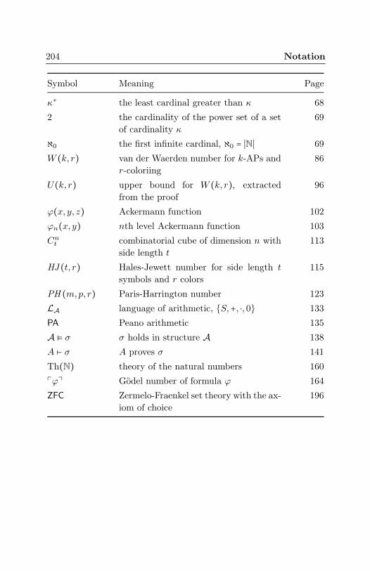
204 Notation
Symbol Meaning Page
κ+ the least cardinal greater than κ 68
2κ the cardinality of the power set of a set
of cardinality κ
69
ℵ0 the first infinite cardinal, ℵ0 = ∣N∣ 69
W (k, r) van der Waerden number for k-APs and
r-coloriing
86
U(k, r) upper bound for W (k, r), extracted
from the proof
96
ϕ(x, y, z) Ackermann function 102
ϕn(x, y) nth level Ackermann function 103
Cnt combinatorial cube of dimension n with
side length t
113
HJ (t, r) Hales-Jewett number for side length t
symbols and r colors
115
PH (m,p, r) Paris-Harrington number 123
LA language of arithmetic, {S,+, ⋅, 0} 133
PA Peano arithmetic 135
A ⊧ σ σ holds in structure A 138
A ⊢ σ A proves σ 141
Th(N) theory of the natural numbers 160⌜ϕ⌝ Godel number of formula ϕ 164
ZFC Zermelo-Fraenkel set theory with the ax-
iom of choice
196

Index
Ackermann function, 102, 105, 106,
108, 110
alephs, 69
arithmetic progression, 85
arrow notation, 2
axiom of choice, 63, 67
Banach-Tarksi paradox, 64
binary string, 46
bounded μ-operator, 107
Burali-Forti paradox, 57
cardinal, 67
inaccessible, 83, 197
limit, 81
Ramsey, 83, 197
regular, 82
singular, 82
strong limit, 81
cardinal arithmetic, 68
cardinality (of a set), 67
Church-Turing thesis, 163
closed, 51
cofinality, 82, 111
coloring, 2
edge, 14
combinatorial
s-space, 118
combinatorial line, 114
compactness, xi, 49, 86, 123, 144
sequentially compact, 52
topological, 52
complete (proof system), 142, 160
complete (theory), 159
computable, 162
continuum hypothesis, 69
generalized, 70, 81
cut, 149
definable, 149, 155
degree (graphs), 6
dominating function, 99
eventually, 99
equivalence relation, 8, 66
free variable, 134
fundamental sequence, 111
Godel β-function, 155, 190
Godel number, 164
Goldbach conjecture, 129
graph, 5
k-partite, 11
bipartite, 10, 31
clique, 10
complement, 6
complete, 9
complete bipartite, 11
connected, 9
cycle, 8
205
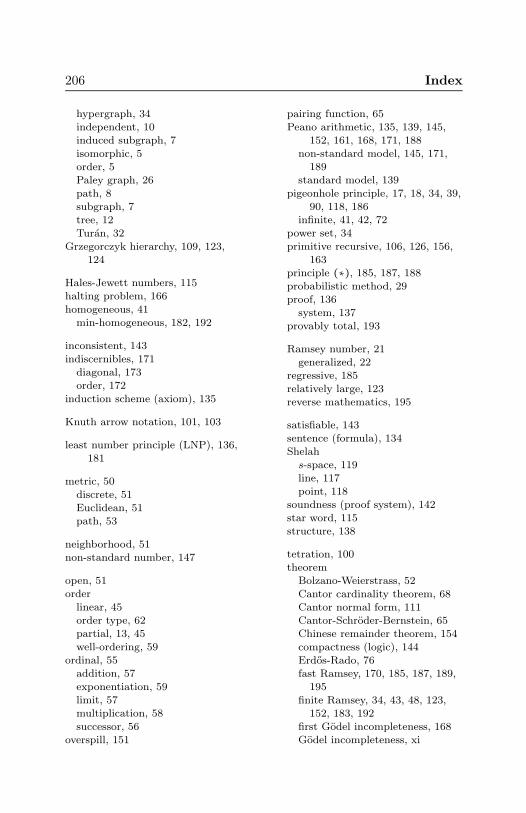
206 Index
hypergraph, 34independent, 10induced subgraph, 7
isomorphic, 5order, 5Paley graph, 26
path, 8subgraph, 7tree, 12
Turan, 32Grzegorczyk hierarchy, 109, 123,
124
Hales-Jewett numbers, 115halting problem, 166
homogeneous, 41min-homogeneous, 182, 192
inconsistent, 143
indiscernibles, 171diagonal, 173order, 172
induction scheme (axiom), 135
Knuth arrow notation, 101, 103
least number principle (LNP), 136,181
metric, 50
discrete, 51Euclidean, 51path, 53
neighborhood, 51non-standard number, 147
open, 51order
linear, 45order type, 62partial, 13, 45
well-ordering, 59ordinal, 55
addition, 57
exponentiation, 59limit, 57multiplication, 58
successor, 56overspill, 151
pairing function, 65Peano arithmetic, 135, 139, 145,
152, 161, 168, 171, 188non-standard model, 145, 171,
189standard model, 139
pigeonhole principle, 17, 18, 34, 39,90, 118, 186
infinite, 41, 42, 72power set, 34
primitive recursive, 106, 126, 156,163
principle (∗), 185, 187, 188probabilistic method, 29proof, 136
system, 137provably total, 193
Ramsey number, 21generalized, 22
regressive, 185
relatively large, 123reverse mathematics, 195
satisfiable, 143sentence (formula), 134Shelah
s-space, 119line, 117point, 118
soundness (proof system), 142
star word, 115structure, 138
tetration, 100theorem
Bolzano-Weierstrass, 52
Cantor cardinality theorem, 68Cantor normal form, 111Cantor-Schroder-Bernstein, 65Chinese remainder theorem, 154
compactness (logic), 144Erdos-Rado, 76fast Ramsey, 170, 185, 187, 189,
195
finite Ramsey, 34, 43, 48, 123,152, 183, 192
first Godel incompleteness, 168Godel incompleteness, xi

Index 207
Godel completeness, 142Greenwood and Gleason bound,
22Hales-Jewett, 113Heine-Borel, 52infinite Ramsey, 41, 52, 71, 124,
172Konig’s lemma, 48, 49, 54, 124Paris-Harrington, xi, 170, 193Ramsey (for graphs), 16, 37Schur, 21second Godel incompleteness,
195, 197Szemeredi, 98Turan, 31, 98unsolvability
Entscheidungsproblem, 167unsolvability of halting problem,
166van der Waerden, ix, 86, 115, 159
tree, 12, 46binary, 46
finitely branching, 47infinite path, 47
Turing machine, 162
van der Waerden number, 86
Wainer hierarchy, 113well-ordering principle, 63
Zermelo-Fraenkel set theory with
choice (ZF), 69Zermelo-Fraenkel set theory with
choice (ZFC), 196

SELECTED PUBLISHED TITLES IN THIS SERIES
87 Matthew Katz and Jan Reimann, An Introduction to Ramsey Theory,2018
86 Peter Frankl and Norihide Tokushige, Extremal Problems for FiniteSets, 2018
85 Joel H. Shapiro, Volterra Adventures, 2018
84 Paul Pollack, A Conversational Introduction to Algebraic NumberTheory, 2017
83 Thomas R. Shemanske, Modern Cryptography and Elliptic Curves, 2017
82 A. R. Wadsworth, Problems in Abstract Algebra, 2017
81 Vaughn Climenhaga and Anatole Katok, From Groups to Geometryand Back, 2017
80 Matt DeVos and Deborah A. Kent, Game Theory, 2016
79 Kristopher Tapp, Matrix Groups for Undergraduates, Second Edition,2016
78 Gail S. Nelson, A User-Friendly Introduction to Lebesgue Measure andIntegration, 2015
77 Wolfgang Kuhnel, Differential Geometry: Curves — Surfaces —
Manifolds, Third Edition, 2015
76 John Roe, Winding Around, 2015
75 Ida Kantor, Jirı Matousek, and Robert Samal, Mathematics++,2015
74 Mohamed Elhamdadi and Sam Nelson, Quandles, 2015
73 Bruce M. Landman and Aaron Robertson, Ramsey Theory on theIntegers, Second Edition, 2014
72 Mark Kot, A First Course in the Calculus of Variations, 2014
71 Joel Spencer, Asymptopia, 2014
70 Lasse Rempe-Gillen and Rebecca Waldecker, Primality Testing forBeginners, 2014
69 Mark Levi, Classical Mechanics with Calculus of Variations and OptimalControl, 2014
68 Samuel S. Wagstaff, Jr., The Joy of Factoring, 2013
67 Emily H. Moore and Harriet S. Pollatsek, Difference Sets, 2013
66 Thomas Garrity, Richard Belshoff, Lynette Boos, Ryan Brown,
Carl Lienert, David Murphy, Junalyn Navarra-Madsen, PedroPoitevin, Shawn Robinson, Brian Snyder, and Caryn Werner,Algebraic Geometry, 2013
65 Victor H. Moll, Numbers and Functions, 2012
For a complete list of titles in this series, visit theAMS Bookstore at www.ams.org/bookstore/stmlseries/.

This book takes the reader on a journey through Ramsey theory, from graph theory and combinatorics to set theory to logic and metamath-ematics. Written in an informal style with few requisites, it develops two basic principles of Ramsey theory: many combinatorial properties persist under partitions, but to witness this persistence, one has to start with very large objects. The interplay between those two principles not only produces beautiful theorems but also touches the very foundations of mathematics. In the course of this book, the reader will learn about both aspects. Among the topics explored are Ramsey’s theorem for graphs and hypergraphs, van der Waerden’s theorem on arithmetic progressions, infi-nite ordinals and cardinals, fast growing functions, logic and provability, Gödel incompleteness, and the Paris-Harrington theorem.
Quoting from the book, “There seems to be a murky abyss lurking at the bottom of mathematics. While in many ways we cannot hope to reach solid ground, mathematicians have built impressive ladders that let us explore the depths of this abyss and marvel at the limits and at the power of mathematical reasoning at the same time. Ramsey theory is one of those ladders.”
For additional information and updates on this book, visit
www.ams.org/bookpages/stml-87
STML/87