An Introduction to NMR-based Metabolomics and Statistical

Data Analysis using MetaboAnalyst

Rohit Mahar (PhD)

Department of Biochemistry and molecular Biology

University of Florida

2

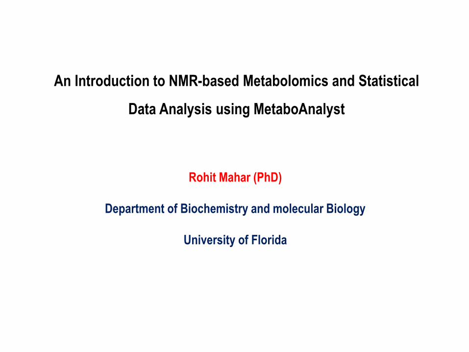
Chemometrics or Multivariate Statistical Analysis: “Chemometrics is the chemical discipline that uses

mathematics and statistics to design experimental procedures for maximum relevant chemical information by

analyzing chemical data and obtain knowledge about chemical systems”

(1) Pattern recognition (2) Sample classification

NMR spectroscopy along with Chemometrics play a vital role in the field of Metabolomics.

General routes of metabolomics

Routes of Metabolomics

3

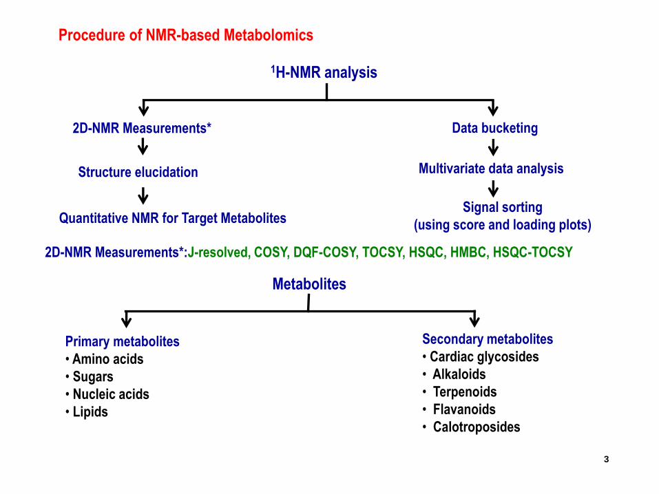
Procedure of NMR-based Metabolomics

2D-NMR Measurements*:J-resolved, COSY, DQF-COSY, TOCSY, HSQC, HMBC, HSQC-TOCSY

Multivariate data analysis

Signal sorting

(using score and loading plots)Quantitative NMR for Target Metabolites

1H-NMR analysis

Data bucketing2D-NMR Measurements*

Structure elucidation

Metabolites

Secondary metabolites

• Cardiac glycosides

• Alkaloids

• Terpenoids

• Flavanoids

• Calotroposides

Primary metabolites

• Amino acids

• Sugars

• Nucleic acids

• Lipids

4

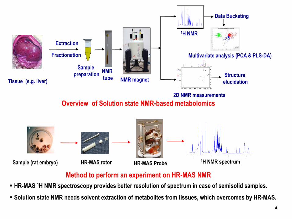
Extraction

Fractionation

Sample

preparation

1H NMR

NMR magnet

2D NMR measurements

Structure

elucidation

NMR

tube

Data Bucketing

Multivariate analysis (PCA & PLS-DA)

Overview of Solution state NMR-based metabolomics

Tissue (e.g. liver)

Sample (rat embryo) HR-MAS rotor HR-MAS Probe

Method to perform an experiment on HR-MAS NMR

1H NMR spectrum

HR-MAS 1H NMR spectroscopy provides better resolution of spectrum in case of semisolid samples.

Solution state NMR needs solvent extraction of metabolites from tissues, which overcomes by HR-MAS.

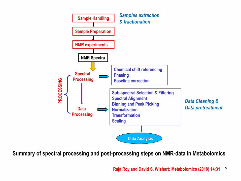
Raja Roy and David S. Wishart; Metabolomics (2018) 14:31

Sample Handling

Sample Preparation

NMR experiments

NMR Spectra

Chemical shift referencing

Phasing

Baseline correction

Sub-spectral Selection & Filtering

Spectral Alignment

Binning and Peak Picking

Normalization

Transformation

Scaling

Spectral

Processing

Data

Processing

PR

OC

ES

SIN

G

Data Analysis

Summary of spectral processing and post-processing steps on NMR-data in Metabolomics

Samples extraction

& fractionation

Data Cleaning &

Data pretreatment

5

6

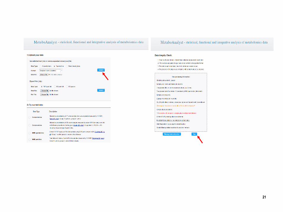
Data Integrity Check:

Checking the class labels - at least three replicates are required in each class.

If the samples are paired, the pair labels must conform to the specified format.

The data (except class labels) must not contain non-numeric values.

The presence of missing values or features with constant values (i.e. all zeros).

7

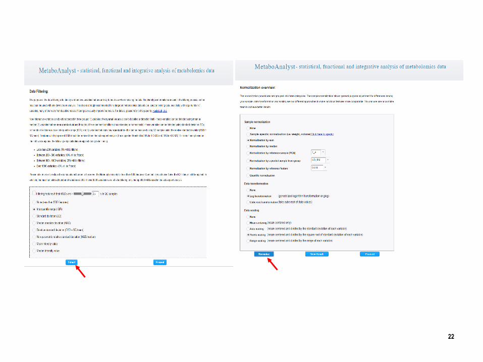
Data Cleaning:

This step is strongly recommended for untargeted metabolomics.

Datasets (i.e. spectral binning data, peak lists) with large number of variables, many of

them are from baseline noises.

Data Filtering methods are used to remove bins that are null and do not displays any

changes among spectra series.

Non-informative variables can be characterized in three groups:

1) Variables of very small values (close to baseline or detection limit) - these variables

can be detected using mean or median.

2) Variables that are near-constant values throughout the experiment conditions

(housekeeping or homeostasis) - these variables can be detected using standard

deviation (SD); or the robust estimate such as interquantile range (IQR).

3) Variables that show low repeatability - this can be measured using the relative

standard deviation (RSD = SD/mean).

8

Rules for Data Cleaning:

Filtering Variable (bin) shows zeros among all rows (spectra) is discarded.

In practice Standard Deviation, Median Absolute Deviation and Interquartile Range are

calculated for all bins.

In Standard Deviation, MAD and IQR a fixed fraction (default 10%) of the bins is discarded

(e.g. if the matrix is composed by 100 bins it means that 10 bins are discarded, and the

selection is based on the Filter method chosen).

An amount of bins (with the lowest SD, or MAD or IQR values) are discarded with respect

a percentage value of the total bins.

The following empirical rules are applied during data filtering:

• Less than 250 variables: 5% will be filtered.

• Between 250 - 500 variables: 10% will be filtered.

• Between 500 - 1000 variables: 25% will be filtered.

• Over 1000 variables: 40% will be filtered.

9

Methods of normalization

Sample normalization (row-wise)

To remove systematic variation between experimental conditions unrelated to the

biological differences (i.e. dilutions, mass).

Feature normalization (column-wise)

To bring variances of all features close to equal.

Normalization: Why normalization is essential?

To ensure that peak intensities are relatively similar from sample to sample.

Correction for sample variation due to sample dilution or sample concentration

(technical or biological).

10

Sample normalization:

Row-wise normalization aims to normalize each sample (row) so that it is comparable to the other.

it is an operation that is performed on the rows of the matrix

Sample-specific normalization (i.e. weight, volume)

Normalization by sum

every element on a row is divided by the sum of all elements of the same row

Normalization by median

every element on a row is reduced by the median value of all the bins that constitute the same row

Normalization by reference sample (PQN)

every element of a row is divided by the corresponding element of the row of the selected

reference spectrum.

A most probable quotient between the signals of the corresponding spectrum and of a reference

spectrum is calculated as normalization factor.

Normalization by a pooled sample from group

If you select a bundle of spectra (like all spectra belonging to the same class) normalization is

performed on the calculated average spectrum.

Normalization by reference feature (selected bin)

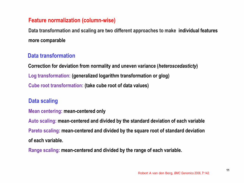
Feature normalization (column-wise)

Data transformation and scaling are two different approaches to make individual features

more comparable

Data transformation

Correction for deviation from normality and uneven variance (heteroscedasticty)

Log transformation: (generalized logarithm transformation or glog)

Cube root transformation: (take cube root of data values)

Data scaling

Mean centering: mean-centered only

Auto scaling: mean-centered and divided by the standard deviation of each variable

Pareto scaling: mean-centered and divided by the square root of standard deviation

of each variable.

Range scaling: mean-centered and divided by the range of each variable.

11Robert A van den Berg, BMC Genomics 2006, 7:142.

12

Interpretation of Scores and Loadings

Relationship of Scores (samples) information to Loadings (variables) information.

Principal Component Analysis (PCA)

Principal Component Analysis (PCA) is a dimension-reduction tool that can be used to reduce a

large set of variables to a small set that still contains most of the information in the large set.

PCA uses orthogonal transformation to convert a set of observations from correlated variables

into a set of values of linearly uncorrelated variables (principal components).

PCA can be used to answer questions such as:

1) What is the pattern of sample distribution?

2) Which variables describe the differences between samples?

3) Which variables contribute most to an observed difference?

4) Which variables contribute in the same way (i.e. are correlated)?

13

PCA model is characterized by three complementary sets of attributes:

Scores

Scores describe the properties of the samples and are usually shown as a map of

one PC plotted against another.

Loadings

Loadings describe the relationships between variables and may be plotted as a

line (commonly used in spectral data interpretation) or a map (commonly used in

process or sensory data analysis).

Explained (or Residual) Variances

These are error measures that tell how much information is taken into account by

each PC.

14

Partial-least squares discriminant analysis (PLS-DA):

PLS-DA is a supervised method that uses multiple linear regression technique to

find the direction of maximum covariance between a data set (X) and the class

membership (Y).

PLS discriminant analysis is used to explain and predict the membership of

observations to several classes using quantitative or qualitative explanatory

variables or parameters.

The quality of the mathematical model was described by the cross-validation

parameters R2 and Q2.

R2 is the goodness of fit and Q2 indicates the predictive ability and indicates the

robustness of model.

Typically, Q2 is lower than R2 for the PLS-DA.

15

PLS-DA tends to overfit the data and therefore the model needs

to be validated to see whether the separation is statistically

significant or is due to random noise.

In each permutation, a PLS-DA model is built between the data (X)

and the permuted class labels (Y) using the optimal number of

components determined by cross validation for the model based

on the original class assignment.

Statistical Data Analysis on Murine’s Urine Samples

Two Groups of samples

1. KO_D3P

2. WT_D1A

16

Case Study

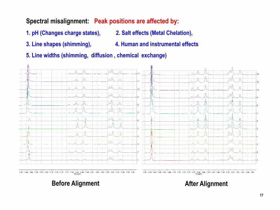
After AlignmentBefore Alignment

Spectral misalignment: Peak positions are affected by:

1. pH (Changes charge states), 2. Salt effects (Metal Chelation),

3. Line shapes (shimming), 4. Human and instrumental effects

5. Line widths (shimming, diffusion , chemical exchange)

17

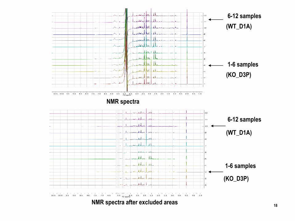
NMR spectra

NMR spectra after excluded areas

1-6 samples

(KO_D3P)

6-12 samples

(WT_D1A)

1-6 samples

(KO_D3P)

6-12 samples

(WT_D1A)

18

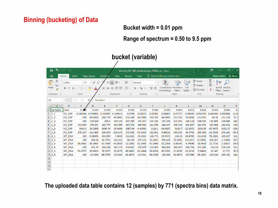
Binning (bucketing) of Data

bucket (variable)

Bucket width = 0.01 ppm

Range of spectrum = 0.50 to 9.5 ppm

The uploaded data table contains 12 (samples) by 771 (spectra bins) data matrix.19

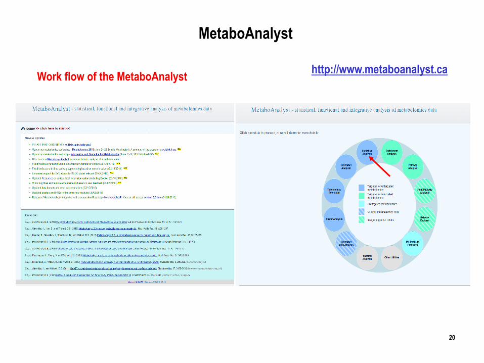
MetaboAnalyst

Work flow of the MetaboAnalyst

20

http://www.metaboanalyst.ca

21

22

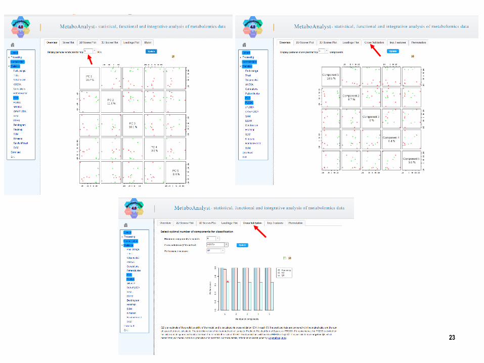
23

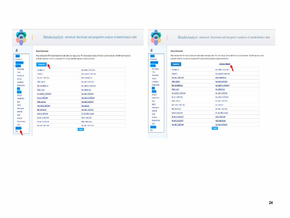
24

25

Statistical Data Analysis of Urine NMR-data recorded

On 600 MHz

26

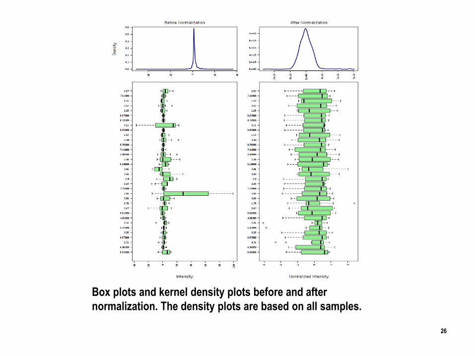
Box plots and kernel density plots before and after

normalization. The density plots are based on all samples.

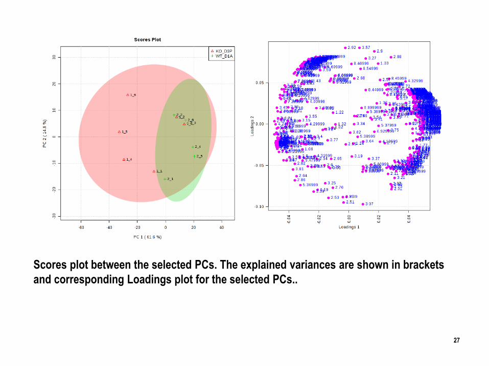
Scores plot between the selected PCs. The explained variances are shown in brackets

and corresponding Loadings plot for the selected PCs..

27

28

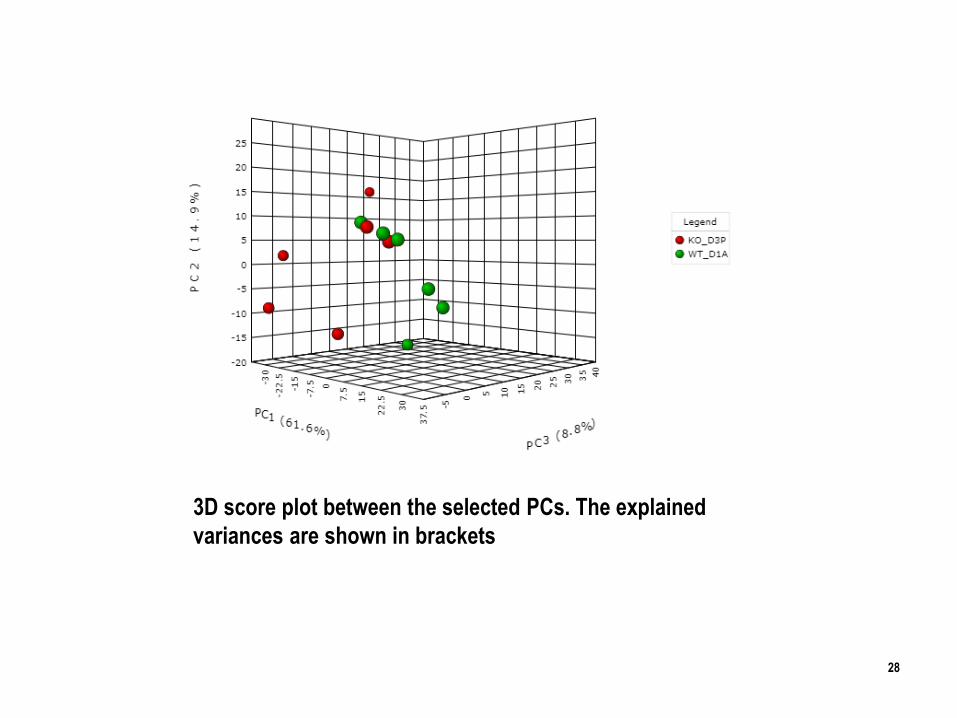
3D score plot between the selected PCs. The explained

variances are shown in brackets

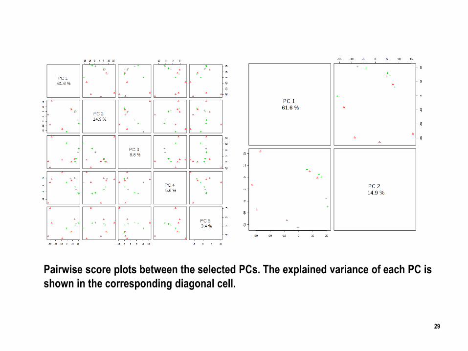
Pairwise score plots between the selected PCs. The explained variance of each PC is

shown in the corresponding diagonal cell.

29

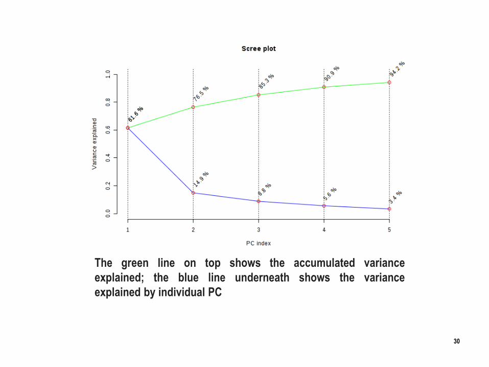
The green line on top shows the accumulated variance

explained; the blue line underneath shows the variance

explained by individual PC

30

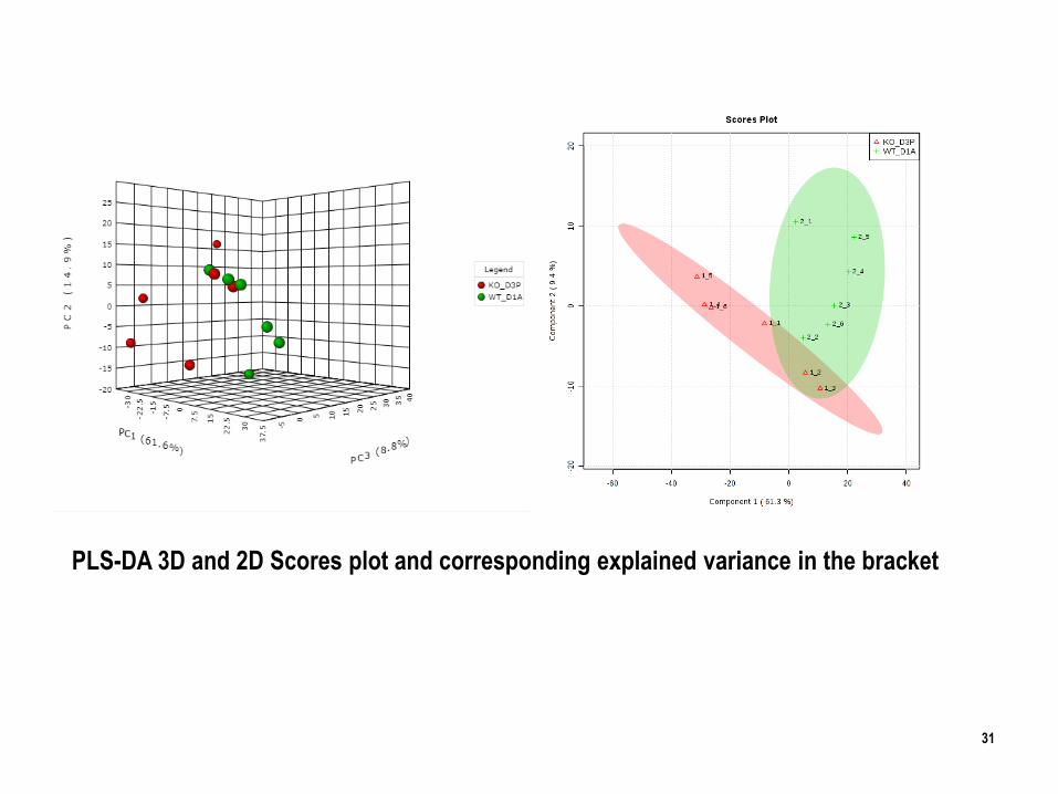
31

PLS-DA 3D and 2D Scores plot and corresponding explained variance in the bracket

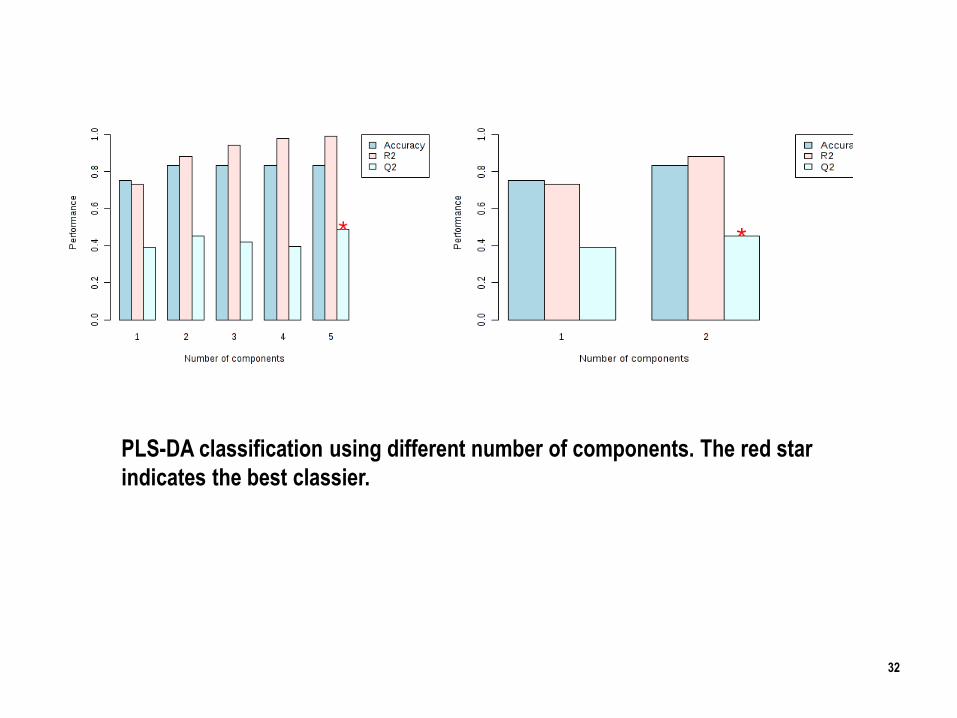
32

PLS-DA classification using different number of components. The red star

indicates the best classier.

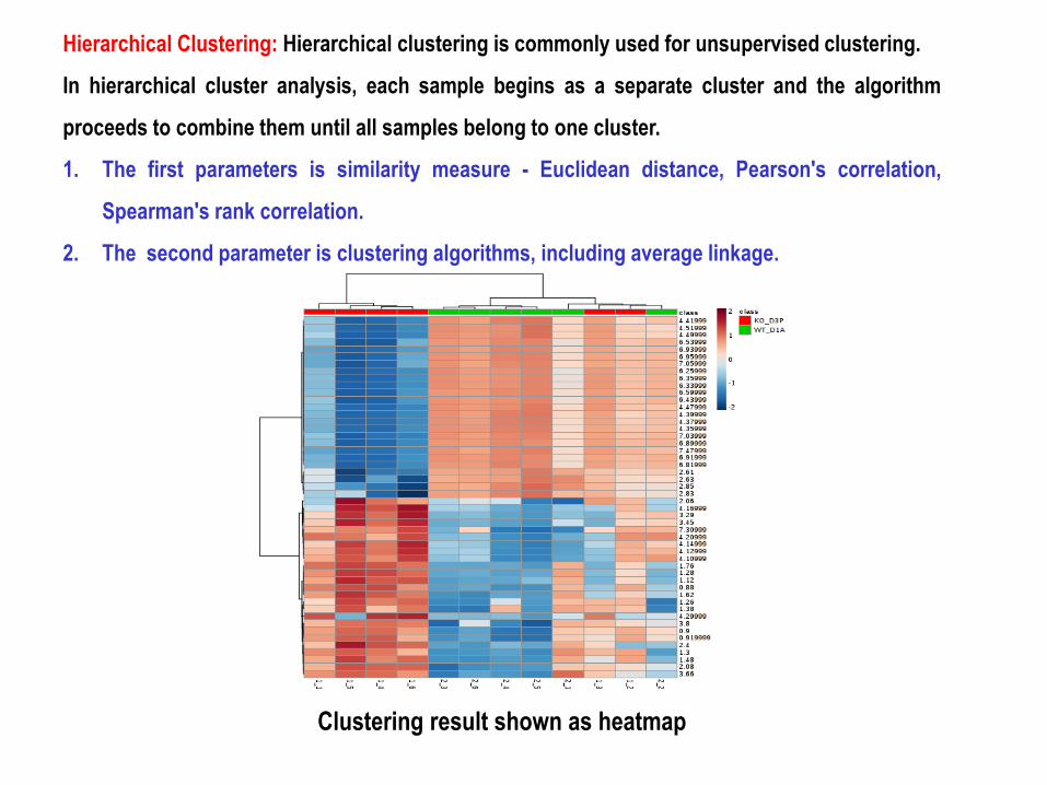
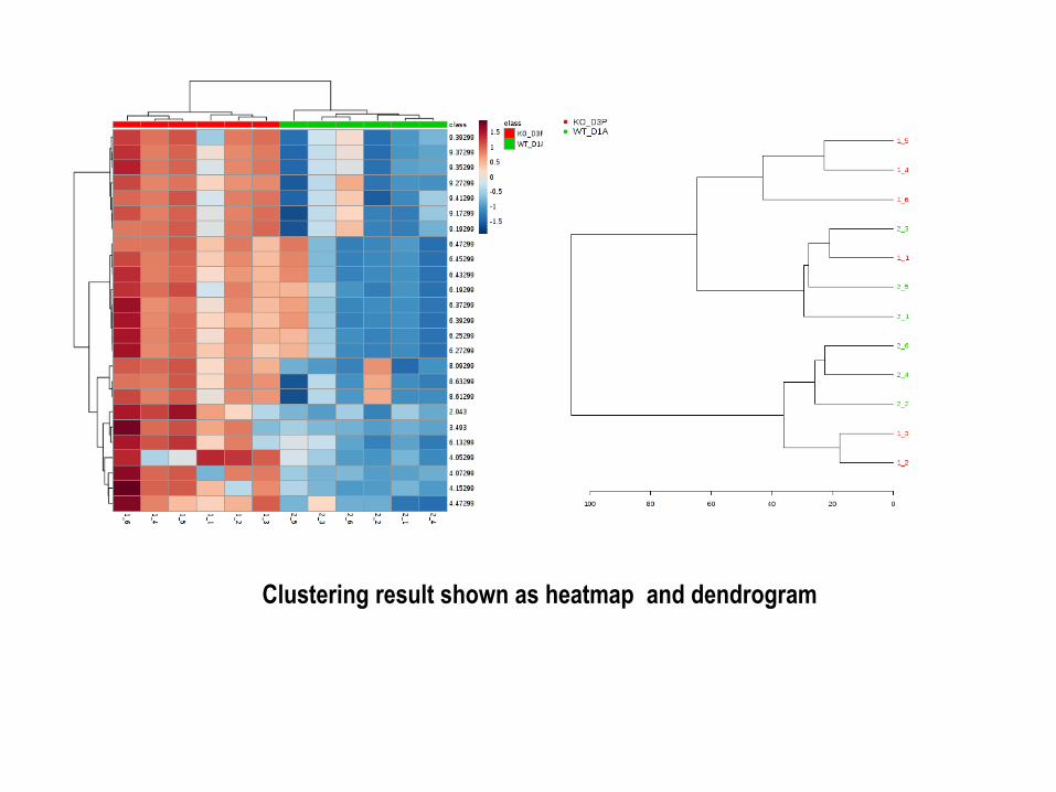
Clustering result shown as heatmap

Hierarchical Clustering: Hierarchical clustering is commonly used for unsupervised clustering.

In hierarchical cluster analysis, each sample begins as a separate cluster and the algorithm

proceeds to combine them until all samples belong to one cluster.

1. The first parameters is similarity measure - Euclidean distance, Pearson's correlation,

Spearman's rank correlation.

2. The second parameter is clustering algorithms, including average linkage.

34

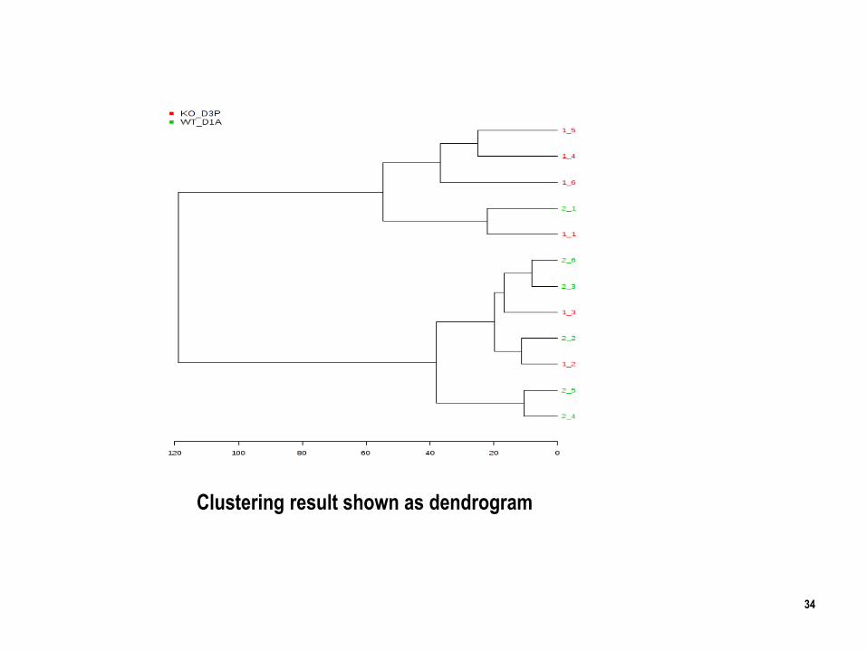
Clustering result shown as dendrogram

35

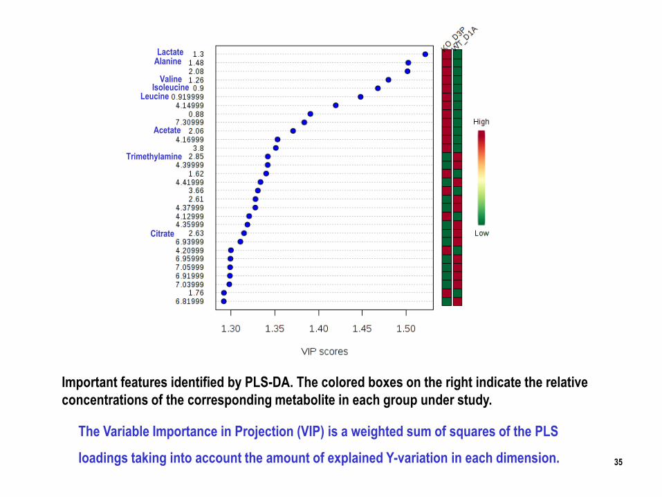
The Variable Importance in Projection (VIP) is a weighted sum of squares of the PLS

loadings taking into account the amount of explained Y-variation in each dimension.

Important features identified by PLS-DA. The colored boxes on the right indicate the relative

concentrations of the corresponding metabolite in each group under study.

Acetate

Alanine

Citrate

Trimethylamine

Lactate

IsoleucineLeucine

Valine

36

Statistical Data Analysis of Urine NMR-data recorded

On 500 MHz

37

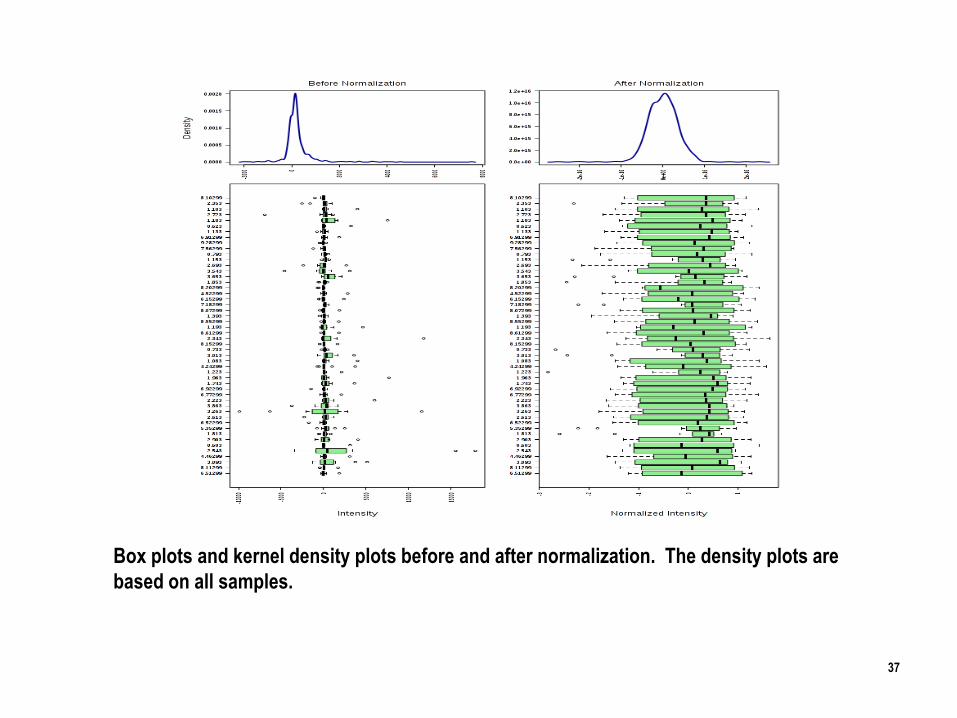
Box plots and kernel density plots before and after normalization. The density plots are

based on all samples.

38

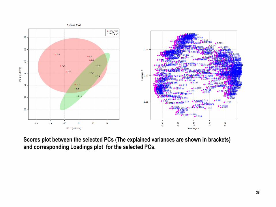
Scores plot between the selected PCs (The explained variances are shown in brackets)

and corresponding Loadings plot for the selected PCs.

39

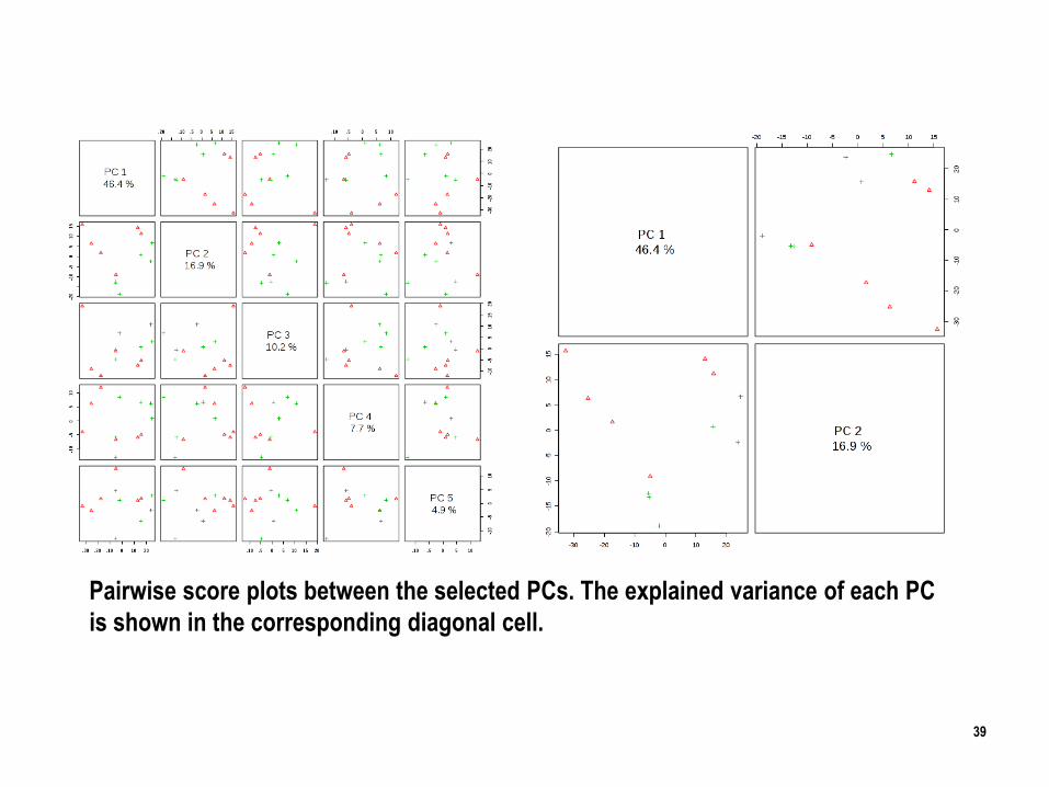
Pairwise score plots between the selected PCs. The explained variance of each PC

is shown in the corresponding diagonal cell.

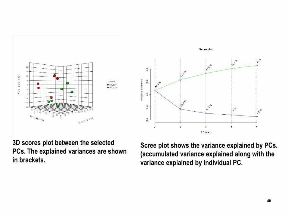
40

Scree plot shows the variance explained by PCs.

(accumulated variance explained along with the

variance explained by individual PC.

3D scores plot between the selected

PCs. The explained variances are shown

in brackets.

41

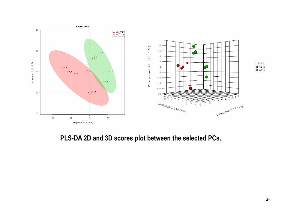
PLS-DA 2D and 3D scores plot between the selected PCs.

42

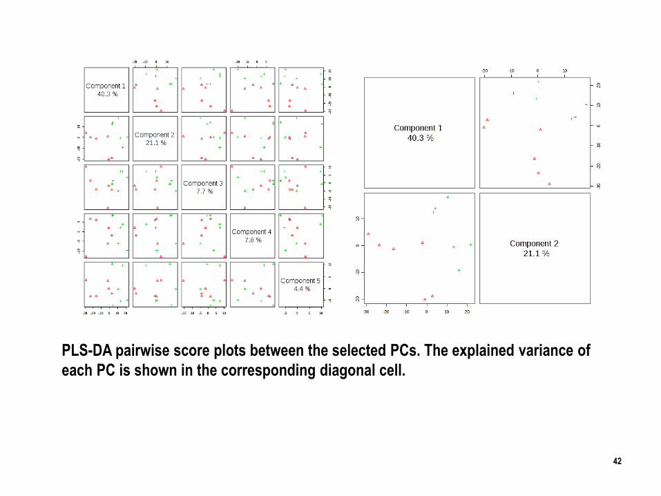
PLS-DA pairwise score plots between the selected PCs. The explained variance of

each PC is shown in the corresponding diagonal cell.

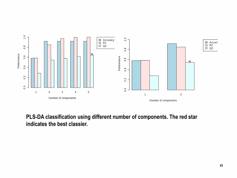
43

PLS-DA classification using different number of components. The red star

indicates the best classier.

Clustering result shown as heatmap and dendrogram

45

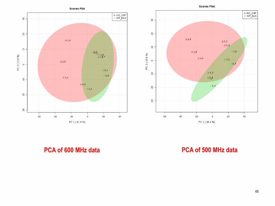
PCA of 500 MHz dataPCA of 600 MHz data

46

47

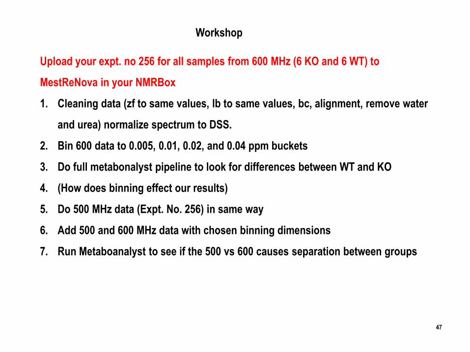
Workshop

Upload your expt. no 256 for all samples from 600 MHz (6 KO and 6 WT) to

MestReNova in your NMRBox

1. Cleaning data (zf to same values, lb to same values, bc, alignment, remove water

and urea) normalize spectrum to DSS.

2. Bin 600 data to 0.005, 0.01, 0.02, and 0.04 ppm buckets

3. Do full metabonalyst pipeline to look for differences between WT and KO

4. (How does binning effect our results)

5. Do 500 MHz data (Expt. No. 256) in same way

6. Add 500 and 600 MHz data with chosen binning dimensions

7. Run Metaboanalyst to see if the 500 vs 600 causes separation between groups