Embed Size (px)
Citation preview

An Introduction to Flow Visualization
Next Time
2
Scientific Visualization
TensorFields
ScalarFields
GeometricMethods
TopologicalVisualization
Feature-Based Texture-Based
VectorFields

An Introduction to Flow Visualization
Lagrangian Flow Analysis
3
Q: Galilean Invariance of FTLE?

An Introduction to Flow Visualization
Lagrangian Flow Analysis
3
Q: Galilean Invariance of FTLE?

An Introduction to Flow Visualization
Lagrangian Flow Analysis
3
Q: Galilean Invariance of FTLE?

An Introduction to Flow Visualization
Lagrangian Flow Analysis
3
The map Φ is called flow map.
Q: Galilean Invariance of FTLE?

An Introduction to Flow Visualization
Lagrangian Flow Analysis
3
The map Φ is called flow map.
Q: Galilean Invariance of FTLE?

An Introduction to Flow Visualization
Lagrangian Flow Analysis
3
!!t(t, x) :=1
!tln
!
"max (Dx #!t(t, x))
Mathematical description:
The map Φ is called flow map.
Q: Galilean Invariance of FTLE?

An Introduction to Flow Visualization
Lagrangian Flow Analysis
3
!!t(t, x) :=1
!tln
!
"max (Dx #!t(t, x))
Mathematical description:
The map Φ is called flow map.
The scalar field σ is called Finite-Time Lyapunov exponent.
Q: Galilean Invariance of FTLE?

An Introduction to Flow Visualization
Lagrangian Flow Analysis
Typical computation:• : Integration of a dense set of pathlines on a regular grid
over the domain of interest
• : numerical derivative + maximum eigenvalue
• Requires high number of pathline computations• Can use GPUs for “simple” data.• Non-simple: adaptive approximation.
!
!
4

An Introduction to Flow Visualization
Lagrangian Flow Analysis
In practice: significant reduction in flow map evaluations
5

An Introduction to Flow Visualization
Lagrangian Flow Analysis
In practice: significant reduction in flow map evaluations
5

An Introduction to Flow Visualization
Incremental Flow Map Approximation
Adaptive resolution of fine detail
6

An Introduction to Flow Visualization
Incremental Flow Map Approximation
Adaptive resolution of fine detail
6

An Introduction to Flow Visualization
Lagrangian Visualization
• Other applications: Medical / DT-MRI• Interest in coherent fiber bundles / bundle separation
Bra
in S
can C
anine Heart
7

An Introduction to Flow Visualization
Lagrangian Visualization
• Other applications: Fusion• Coherent Structures: Island Chain Boundaries
8

An Introduction to Flow Visualization 9

An Introduction to Flow Visualization
Next Time
10
Scientific Visualization
TensorFields
ScalarFields
GeometricMethods
TopologicalVisualization
Feature-Based Texture-Based
VectorFields

An Introduction to Flow Visualization 11
Features?
• Vortices
• Flow separation and attachment

An Introduction to Flow Visualization 12
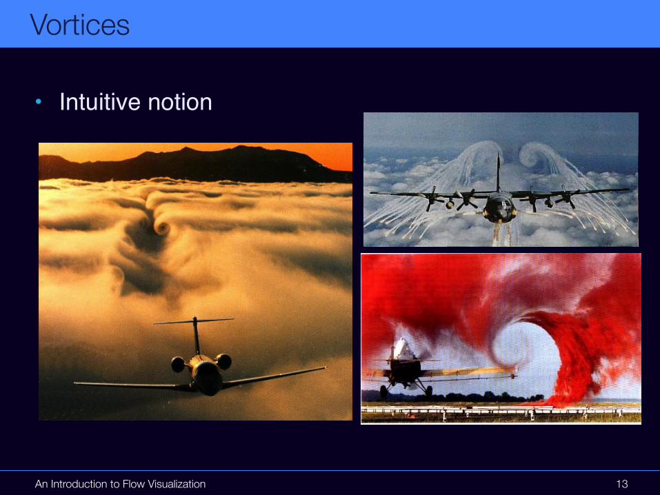
Vortices
• Intuitive notion
http://www.cse.ohio-state.edu/~jiang/Vortex/ieeeVis02.ppt
An Introduction to Flow Visualization 13
Vortices
• Intuitive notion

An Introduction to Flow Visualization 14
Vortices
• “A vortex is the rotating motion of a multitude of material particles around a common center“
H. J. Lugt, The dilemma of defining a vortex, Recent Developments in Theoretical and Experimental Fluid Mechanics, Springer, 1979
• “A vortex exists when its streamlines, mapped onto a plane normal to its core, exhibit a circular or spiral pattern, under an appropriate reference frame.”S. K. Robinson, Coherent motions in the turbulent boundary layer, Ann. Rev. Fluid Mech., vol. 23, 1991
• “A vortex is comprised of a central core region surrounded by swirling streamlines.”
L. M. Portela, Identification and characterization of vortices in the turbulent boundary layer. Ph.D. thesis, Stanford University, 1997

An Introduction to Flow Visualization
Vortices
Rotation around axis + Motion along axis = Vortex
15
+ =
Center of rotational motion is called vortex core line.
“Region of influence” of the vortex core line is called vortex core.

An Introduction to Flow Visualization
Vortex Extraction from CFD Data
• Based on specific feature definition, usually from one of two categories:
• Region-Type → Vortex Cores• subset of a dataset where a certain criterion
holds for the whole subset
• Line-Type → Vortex Core Lines• (connected) line segments indicate the center line of rotation• allows for a abstract representation of vortices (skeleton)
16

An Introduction to Flow Visualization
Vortex Extraction from CFD Data
Specific application example: delta-wing aircraft
Vortices are key:• main source of lift and
good maneuverability • primary, secondary, tertiary
vortices form a system abovethe wing
17
An Introduction to Flow Visualization
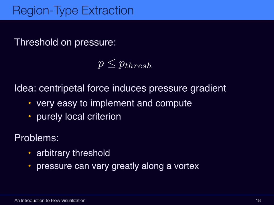
Region-Type Extraction
Threshold on pressure:
Idea: centripetal force induces pressure gradient• very easy to implement and compute• purely local criterion
Problems:• arbitrary threshold• pressure can vary greatly along a vortex
18
p ≤ pthresh

An Introduction to Flow Visualization
Region-Type Extraction
Threshold on pressure
19

An Introduction to Flow Visualization
Region-Type Extraction
Threshold on vorticity magnitude:
Idea: strong infinitesimal rotation• common in fluid dynamics community• very easy to implement and compute, purely local
Problems:• arbitrary threshold• vorticity often highest near boundaries• vortices can have vanishing vorticity
20
|∇× v| ≥ ωthresh

An Introduction to Flow Visualization
Region-Type Extraction
Threshold on vorticity magnitude
21

An Introduction to Flow Visualization
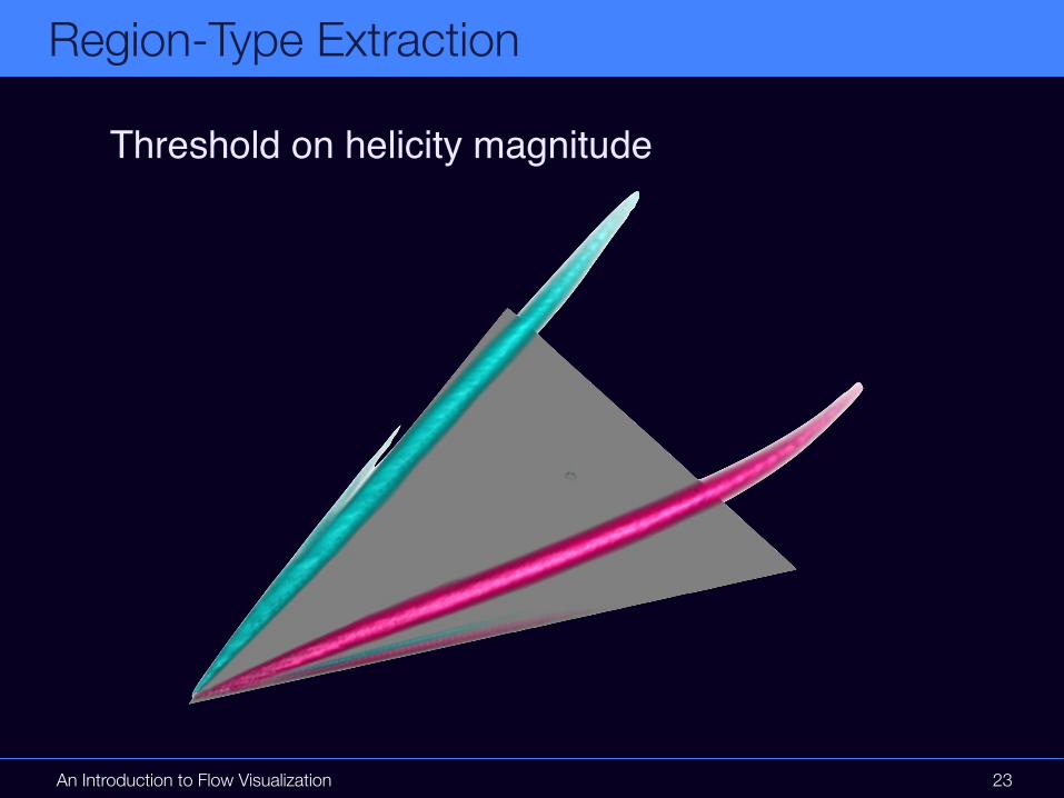
Region-Type Extraction
Threshold on (normalized) helicity magnitude:
Idea: use vorticity but exclude shear flow• still easy to implement and compute, purely local
Problems:• arbitrary threshold• fails for curved shear layers• vortices can have vanishing vorticity
22
|(∇× v) · v| ≥ hthresh
An Introduction to Flow Visualization
Region-Type Extraction
Threshold on helicity magnitude
23

An Introduction to Flow Visualization
Region-Type Extraction
Q-criterion (Jeong, Hussain 1995) positive 2nd invariant of Jacobian
Idea: Q > 0 implies local pressure smaller than surrounding pressure. Condition can be derived from characteristic polynomial of the Jacobian.
• common in CFD community
• can be physically derived from kinematic vorticity (Obrist, 1995)
• need good quality derivatives, can be hard to compute
24
Q = J11J22 − J12J21 + J11J33 − J13J31 + J22J33 − J23J32

An Introduction to Flow Visualization
Region-Type Extraction
Q > 0
25

An Introduction to Flow Visualization
Region-Type Extraction
-criterion
Define as the second largest eigenvalue of
Vortical motion where .• precise threshold, nearly automatic• very widely used in CFD• susceptible to high shear• insufficient separation of close vortices
shear contribution of J rotational contribution of J
26
λ2
S :=1
2(J + JT ) Ω :=
1
2(J − JT )
λ2
S2 + Ω2
λ2 < 0

An Introduction to Flow Visualization
Region-Type Extraction
27

An Introduction to Flow Visualization
A Brief Survey of Methods
Line-Type Methods
28

An Introduction to Flow Visualization
Line-Type Extraction
Line-type vortex core extraction methods allow a further classification into several types:
• pattern matching(based on a specific physical pattern)
• geometric(involving the geometry of streamlines/surfaces)
• integration-based(extraction of core lines as integral curves)
• topological(identifying vortex core lines as part of the topological skeleton of a dataset)
None of these classes is a priori superior to the others.29

An Introduction to Flow Visualization
Line Type Extraction
Banks-Singer (1994):
Idea: Assume a point on a vortex core is known.
• Then, take a step in vorticity direction (predictor).
• Project the new location to the pressure minimum perpendicular to the vorticity (corrector).
• Break if correction is too far from prediction.
9
We next refine the position of the seed point so that it is not constrained to lie on the grid.
The seed point moves in the plane perpendicular to the vorticity vector until it reaches the
location of the local pressure minimum. From this seed point we develop the vortex skeleton
in two parts, forward and backward, to reach the endpoints of the vortex tube.
3.2 Growing the Skeleton
The predictor-corrector algorithm is illustrated in the schematic diagrams of fig. 2. The details
for continuing the calculation from one point to the next are indicated by the captions. Steps
1-2 represent the predictor stage of the algorithm. The corrector stage is summarized by steps
3-4.
Once a seed point has been selected, the skeleton of the vortex core can be grown from the seed.
The next position of the vortex skeleton is predicted by integrating along the vorticity vector (fig. 2,
top) which is equivalent to Euler integration of a vorticity line. The predicted point typically misses the
vortex core.
Next we invoke the heuristic that centripetal acceleration within a vortex is supported by low pres-
sure at the core. In a plane perpendicular to the core, the pressure minimum is expected to coincide
with the point where the core pierces the plane. The predicted point must be corrected to the pressure
minimum in the plane that (1) is perpendicular to the core and (2) contains the predicted point. The
location of the nearest core point is the unknown quantity, so condition (1) can only be satisfied
approximately. We approximate the desired plane by choosing the plane perpendicular to the vorticity
vector (fig. 2, bottom).
pi!i
pi+1
pi+1
(1) (2)
(3) (4)
Figure 2.
Four steps of the predictor-corrector
algorithm.
P
!i+1
Compute the vorticity at apoint on the vortex core.
Step in the vorticity directionto predict the next point.
Compute the vorticity atthe predicted point.
Correct to the pressure minin the perpendicular plane.
Image from Banks, Singer, Vis 1994
30

An Introduction to Flow Visualization
Line Type Extraction
Banks-Singer, contʼd.
Results in core lines that are roughly vorticity lines and pressure valleys.
• Seeding point set can be large(e.g. local pressure minima)
• Requires additional logic to identify unique lines
31

An Introduction to Flow Visualization
3 Line-Type Features: The State of the Art 3.4 Lin e-Ty p e D e fin itio ns o f th e V ort ex C or e
46
By traversing all tetrahedra, the algorithm builds a list of straight line segments which in their
entirety make up the vortex cores of the data set extracted by the algorithm. Obviously, the cal-
culation for each tetrahedron is independent, so this is a trivially parallelizable algorithm. It is
important to note that the line segments produced by this algorithm do not connect to a (poly-)
line due to the chosen piecewise linear interpolation (constant Jacobian), which causes discon-
tinuities (jumps) in the Jacobian across each face of the tetrahedrization and causes mismatch
in the vortex cores on the two sides of the face unless the field is truly linear across both tetra-
hedra.
We will further analyze this algorithm and its underlying definition of a vortex core in section
5.2.5. We will see that the definition can be put in much simpler terms than reciting the above
algorithm. Also, we will see that the algorithm preforms perfectly for all globally linear vector
fields.
The eigenvector method was applied in a 1997 case study by Kenwright and Haimes [67],
depicted in Fig. 3.17. Especially the video sequences presented in this case study, where the
vortex core method is applied to a large time-dependent aerodynamic simulations, impressively
illustrate the merits of feature-based visualization to find essential features in huge data sets.
Interestingly, the method is able to represent a skeleton of continuous vortex cores reasonably
in spite of the fact that the method produces a set of line segments which are not continuous, but
amost aligned in areas where the vortex core is straight.
Fig. 3.16: Sketch of steps in the Sujudi/Haimes algorithm.
velocities reduced velocities core segment
line of zero
reduced velocity
direction of real
eigenvector
Line Type Extraction
Sujudi-Haimes (1995)Idea: pattern matching on tetrahedral cells• identify cells with complex eigenvalue pair in the Jacobian
(indicates rotation)
• subtract remaining eigenvector
• compute center of rotation on cell faces and connect by a line segment
Figure from M. Roth, PhD thesis 32

An Introduction to Flow Visualization
Line Type Extraction
Sujudi-Haimes
33

An Introduction to Flow Visualization
Line Type Extraction
Sujudi-Haimes, contʼd.
• de-facto standard method in CFD• criterion is local per cell and readily parallelized• resulting line segments are disconnected
(Jacobian is assumed piecewise linear)• numerical derivative computation can cause noisy results• has problems with curved vortex core lines
(sought-for pattern is straight)
34

An Introduction to Flow Visualization
Line Type Extraction
Plethora of other pattern matching schemes:• Miruda-Kida
(sectional minima of pseudo-pressure)
• Strawn-Kenwright-Ahmda(lines of max. vorticity magnitude perp. to vorticity)
• Levi-Degani-Seginer(lines where normalized helicity approaches +-1)
Most of these schemes are rarely usedand complex to implement.
35
An Introduction to Flow Visualization
Line Type Extraction
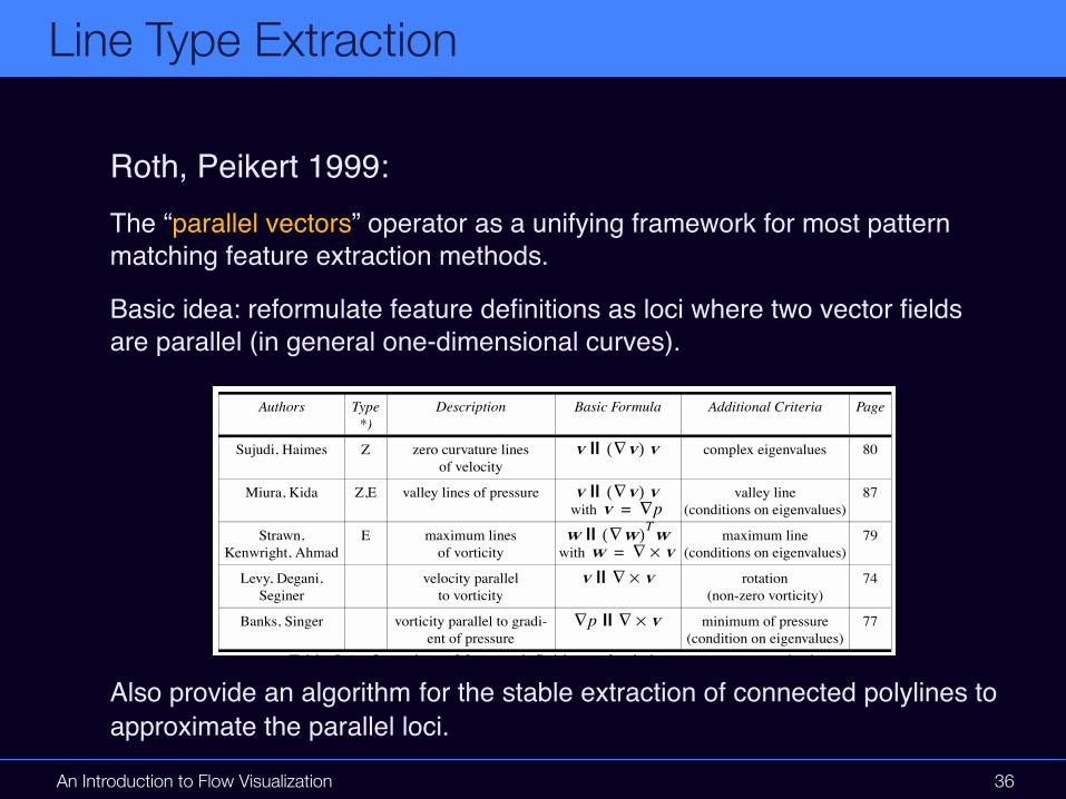
Roth, Peikert 1999:The “parallel vectors” operator as a unifying framework for most pattern matching feature extraction methods.
Basic idea: reformulate feature definitions as loci where two vector fields are parallel (in general one-dimensional curves).
Also provide an algorithm for the stable extraction of connected polylines to approximate the parallel loci.
5 Analysis of Line-Type Features 5.3 Syst e m a ti c O v e rv i e w
88
So we can put the same definition in much simpler words: the vortex cores are the valley lines
of (pseudo-) pressure. We can also use one of the standard parallel vectors operator implemen-
tations to find the vortex core lines without having to resort to approximations and needing arbi-
trary thresholds.
5.3 Systematic Overview
In the last section, we saw how each of the line-type features from chapter 5 can be expressed
using the parallel vectors operator. We also saw that there are generalized features, namely min-
imum and maximum lines, the loci of zero curvature and ridge and valley lines.
Table 5-1 lists the methods for vortex core lines. Each of the methods can be expressed using
the parallel vectors operator combined with some Boolean criteria, typically on the eigenvalues.
The parallel vectors operator allows us to express each of these definitions in a common math-
ematical language, which also is very compact compared with the original descriptions of each
of these methods. It also allows to use a common implementation in the form of a set of modules
such as the collection of AVS 5 modules we published (appendix D).
In the following, we organize the various feature definitions into a hierarchy. Fig. 5.7 attempts
to visualize this hierarchy as three related trees. On the left are line-type features of a scalar data
set, in the center are those of a vector data set. On the right are line-types features of a data set
consisting of two vector fields.
Each box represents a particular class of feature definitions, referred by name and sometimes
by the formula. Subsets are below their superset, slightly indented and connected to their super-
set by a line. Since Fig. 5.7 attempts to capture one of the most important results of this research
project, we will in the following describe how to interpret it.
Authors Type
*)
Description Basic Formula Additional Criteria Page
Sujudi, Haimes Z zero curvature lines
of velocity
complex eigenvalues 80
Miura, Kida Z,E valley lines of pressure
with
valley line
(conditions on eigenvalues)
87
Strawn,
Kenwright, Ahmad
E maximum lines
of vorticity with
maximum line
(conditions on eigenvalues)
79
Levy, Degani,
Seginer
velocity parallel
to vorticity
rotation
(non-zero vorticity)
74
Banks, Singer vorticity parallel to gradi-
ent of pressure
minimum of pressure
(condition on eigenvalues)
77
Table 5-1: Overview of feature definitions of existing vortex core methods
Type *): Z = zero curvature lines, E = extremum lines
v || !v( ) v
v || !v( ) vv !p=
w || !w( )Tww ! v"=
v || ! v"
!p || ! v"
36

An Introduction to Flow Visualization
Line Type Extraction
Sahner et al. 2005
Idea: construct a special vector field that allows to model ridge/valley-lines as integral curves (“feature flow field”).Authors applied it to Q-criterion and λ2-criterion. • Works well in practice
• Feature flow field requires high-order partial derivativesdifficult to compute in certain dataset types
• Seed point set required (usually minimal points)
37

An Introduction to Flow Visualization
Line Type Extraction
Sahner et al. / Galilean Invariant Vortex Core Lines
(a) Visualized using illuminated field lines [ZSH96] and a
LIC-textured stream surface [BSH96]. Vortex core lines following
the approach of [SH95, PR99] displayed as gray lines.
(b) Isosurfaces of λ2.
(c) Galilean invariant vortex core lines. (d) Comparison between λ2-isosurfaces and our vortex core lines.
View from top.
Figure 5: Bubble chamber. Vortex core lines extracted, colored and scaled according to λ2. Same colormap as in figure 4.
of 200 and at a spanwise wavelength of 4 diameters. This
flow exhibits periodic vortex shedding leading to the well
known von Kármán vortex street. This phenomenon plays an
important role in many industrial applications, like mixing
in heat exchangers or mass flow measurements with vortex
counters. However, this vortex shedding can lead to undesir-
able periodic forces on obstacles, like chimneys, buildings,
bridges and submarine towers. The chain of vortices with
their alternating orientation of rotation is clearly depicted in
figure 4 due to the usage of spiraling orbits. This is a major
property of the von Kármán vortex street. Furthermore, it can
be seen that downstream the vortices loose their strength.
Figure 5 shows the geometry of a bubble chamber and its
interior flow. The flow has been measured experimentally on
a 11× 11× 10 uniform grid by a biplanar x-ray angiogra-
phy in a biofluidmechanics laboratory. The bubble chamber
is used as a biochemical reactor. Air injection into the liquid
through holes in the floor plate is used to improve the re-
action. The dataset was provided by Axel Seeger, Biofluid-
mechanics Lab, Charite Berlin. Figure 5a shows a Galilean
variant vortex core line according to [SH95, PR99] around
which the flow spirals. Figure 5b shows isosurfaces of λ2
corresponding to different isovalues. In Figure 5c, the vor-
tex core lines with respect to λ2 extracted by our method are
c The Eurographics Association 2005.
Sahner et al. / Galilean Invariant Vortex Core Lines
(a) Original frame of reference. Vortex core lines following theapproach of [SH95, PR99].
(b) Alternative frame of reference. Vortex core lines following theapproach of [SH95, PR99].
(c) Our Galilean invariant approach. Vortex core lines extracted asvalley lines of λ2.
Figure 1: Flow behind a circular cylinder. Vortex regionsvisualized as transparent isosurfaces of λ2. Vortex core linesdisplayed as cylindrical lines.
variant part, i.e., they depend on a certain frame of refer-ence (Figures 1a-b). In contrast to vortex region detectiondescribed above, the extraction of those lines is parame-ter free in the sense that their definition does not refer toa range of values. This eliminates the need of choosingcertain thresholds.
In this paper we present an approach to extracting vortexcore lines that is invariant under Galilean changes of the ref-erence frame. I.e., the extracted features remain unchangedwhen a constant vector is added to the flow field. Instead ofusing swirling stream line behavior as indication of a vor-tex core line, we consider ridge or valley lines of Galileaninvariant vortex region quantities (Figure 1c). Furthermore,we show that those line type features have a higher dimen-sional generalization, e.g., surfaces.
The article is organized as follows: sections 2.1 and 2.2review the most important approaches to vortex region de-tection and vortex core line extraction. While section 2.3treats the theory of ridge and valley lines, section 3 dealswith implementation issue for their extraction. In Section 4we present an iconic representation for vortex core lines thatencodes the most relevant information like strength of thecoherent structure as well as rotation direction. We apply ourtechnique to several data sets in section 5.
2. Theoretical Background
We now give a short introduction to the two vortex detectionapproaches mentioned above and suggest a combination ofboth in subsection 2.3.
2.1. Vortex Region Detection
There are several derived scalar quantities that indicate vor-tex activities. Ranging from simple to involved, vorticesmight be defined as regions of high magnitude of vorticityω = (ω1,ω2,ω3)t =∇×v, low pressure p, rotation strength∆, positive Q-criterion and negative λ2-criterion. In the fol-lowing, we give some details on the three latter quantities.
Rotation strength ∆ as used in [SP03], see also [CPC90]is linked to the intuitive understanding that a vortex exhibitsspiraling stream lines with respect to some specific referenceframe. Within this reference frame, the stream line pattern ofa flow field is dominated by its Jacobian Jv. If J has a conju-gate pair of complex eigenvalues, the flow locally spirals in aplane corresponding to those eigenvectors. ∆ is then definedas the magnitude of the imaginary part of those complexconjugate eigenvalues. So large values of ∆ indicate strongspiraling patterns within the right reference frame. Where∆ = 0, no such reference frame can be found. By consideringthe orientation of the corresponding eigenbasis, a rotationangle ϕ ∈ (−π,π) can also be extracted. When ϕ > 0, theflow spirals counter clockwise around the eigenvector corre-sponding to the real eigenvalue, clockwise, if ϕ < 0.
The closely linked quantities Q and λ2 are related to theNavier Stokes equations and reflect the amount of strain andvortical motions in the vector field. Due to this fact thosequantities are the most popular among fluid mechanicists.Let∇v denote the gradient of the vector field. Then the straintensor S is defined as its symmetric part S = 1
2 (∇v +∇vt).
c The Eurographics Association 2005.
38
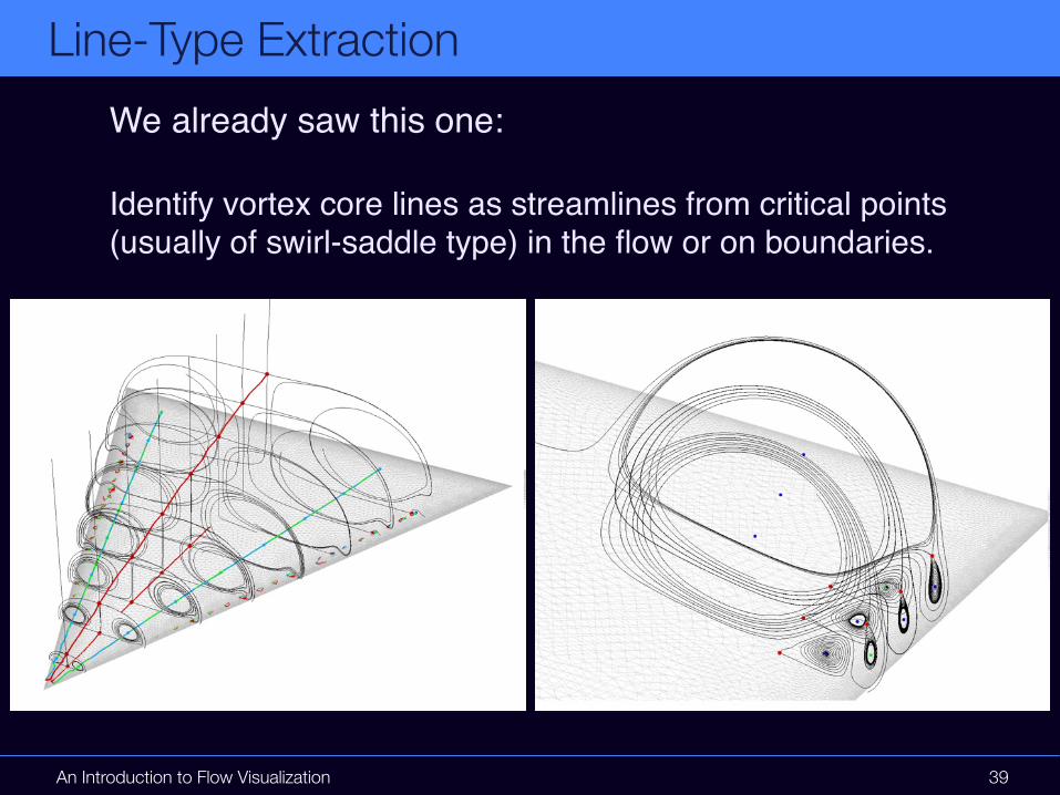
We already saw this one:
Identify vortex core lines as streamlines from critical points (usually of swirl-saddle type) in the flow or on boundaries.
An Introduction to Flow Visualization
Line-Type Extraction
39

An Introduction to Flow Visualization
Line-Type Extraction
Geometric methods:• Jiang et al. 2002:
Combinatorial topology approach (based on Spernerʼs lemma and Poincaré index theory)
• Jiang et al. 2002:Purely geometric verification ofvortex core lines
Purely geometric methods are mostlyuseful for verification tasks and are often computationally intensive.
Jiang, Machiraju, and Thompson / A Novel Approach To Vortex Core Region Detection
Figure 13: Bent-helical vortex
Figure 14: Blunt fin vortices
Figure 15: Delta wing vortices
c The Eurographics Association 2002.
Figure 5: Steady progression of the verification process for theRankine vortex: (left) one-third and (right) two-third of a completespiral.
probe vectors. And Figure 4(c) is the tangent space, in which thetangent vectors are projected onto the (x,y)-plane to generate thetangent profile.
To illustrate the geometric verification process, we seeded astreamline near the vortex core and traced it for one-third of a spiral,and then for another one-third. This is illustrated in Figure 5. Fig-ure 5(left) illustrates the first third and Figure 5(right), the secondthird. Note the steady progression of the tangent profile around the(x,y)-plane as the streamline spirals around the vortex core. Eachcomplete spiral corresponds to a complete revolution in the (x,y)-plane of the tangent space.
5.2 Bent Helical Vortex
The bent helical vortex is an important model for turbomachineryflow fields [14]. The model consists of a helical flow field built froma rigid rotation in the (x,z)-plane, a constant motion in y-directionand a bent of radius R in the (x,y)-plane. The velocity field for thebent helical vortex is given in the (x,y,z) coordinate system by
ux = !! x z Rr2
! " yr
uy = !! y z Rr2
+ " xr
uz =!R ! R2
r
"!
(2)
where r =#x2+ y2.
R is the radius to which the vortex core is bent, " is the axialcomponent along the core, and ! is the rotation component aboutthe core. This flow field has zero divergence (i.e. it conserves massfor a incompressible medium), but it is not an exact solution ofthe Navier-Stokes equations, and it possesses a singularity on thez-axis. However, in the vortex core region there are no singulari-ties or critical points, and similar flow patterns have been found innumerical solutions from a Navier-Stokes solver [14].
Figure 6: Bent helical vortex [14]
Figure 6 illustrates a bent helical vortex with R = 1, ! = 6 and" = 0.5. The velocity field was generated on a 1283 cartesian grid.The yellow region represents the detected vortex core, and the bluelines, the swirling streamlines. Clearly, the vortex core is curvedwith a nontrivial curvature. To illustrate the efficacy of our localalignment transformation, we seed a streamline near one end ofthe bent vortex core and compute its tangent space both with andwithout the transformation. Figure 7(left) illustrates the streamline,along with its tangent vectors and probe vectors. Figure 7(right)illustrates both tangent spaces. The difference between the two isquite clear: without transformation, the tangent vectors can pointin various directions without any particular order, and with trans-formation, the tangent vectors uniformly revolve around the z-axis,forming a cone shape with its apex at the origin of the tangent space.
Figure 7: Difference between tangent profiles with (bottom) andwithout (top) the local alignment transformation.
To demonstrate the effectiveness of our geometric verificationalgorithm on slowly rotating, curved vortices, we conducted severalexperiments using the bent helical vortex model, with R = 1, " =0.5, and ! varying from 6 down to 1. Figure 8(left) illustrates theresults for ! = 4, and Figure 8(right), the results for ! = 2. For! < 1, the tangent profiles did not satisfy the 2# swirling criterion(i.e. they did not complete a revolution in the (x,y)-plane).
40

Garth et al. 2005: hybrid geomtric/integration-based
Extraction using stream surfaces.
Idea: Assume that the locationof a vortex is roughly known(application-specific knowledgeor obtained from other scheme).Then...
An Introduction to Flow Visualization
Line-Type Extraction - Hybrid Approaches
41

Determine center of rotation on a plane roughly perpendicular to the presumed core line (critical point in the plane)
An Introduction to Flow Visualization
Line-Type Extraction - Hybrid Approaches
42

Surround the center with a circular curve and integrate a stream surface from this curve.
An Introduction to Flow Visualization
Line-Type Extraction - Hybrid Approaches
43

While the stream surface exhibits rotating behavior, extract its center of gravity line as an approximation of the vortex core line.
An Introduction to Flow Visualization
Line-Type Extraction - Hybrid Approaches
t0 t1 t2 t3
44

An Introduction to Flow Visualization
Line-Type Extraction - Hybrid Approaches
45

An Introduction to Flow Visualization
Line-Type Extraction - Hybrid Approaches
Garth et al. contʼd.
Further contribution: grow vortex region from vortex core line using the physical Rankine vortex model:
circumferential velocity
center
radius
vortex core boundary
46

An Introduction to Flow Visualization
Line-Type Extraction - Hybrid Approaches
47

An Introduction to Flow Visualization
Open Topics
Did not touch a number of relevant issues here:
• Growing CFD datasets with complex geometries• can possibly have 100s or 1000s of vortices• challenge for both algorithms and visualization• scale dependence – large vortices lost in small-scale noise
• Exact and general vortex definition• Haller 2005: “An objective vortex criterion” –
interesting, but extremely complex
• Frame-of-reference dependence / Galilean invariance• for most methods, results change heavily if FOR change
• Tracking over time?• available for some methods
λ248