Embed Size (px)
Citation preview
HAL Id: hal-00558477https://hal.archives-ouvertes.fr/hal-00558477
Submitted on 21 Jan 2011
HAL is a multi-disciplinary open accessarchive for the deposit and dissemination of sci-entific research documents, whether they are pub-lished or not. The documents may come fromteaching and research institutions in France orabroad, or from public or private research centers.
L’archive ouverte pluridisciplinaire HAL, estdestinée au dépôt et à la diffusion de documentsscientifiques de niveau recherche, publiés ou non,émanant des établissements d’enseignement et derecherche français ou étrangers, des laboratoirespublics ou privés.
An introduction to finite volumes for gas dynamicsFrançois Dubois
To cite this version:François Dubois. An introduction to finite volumes for gas dynamics. Vladimir V. Shaidurov et OlivierPironneau. Encyclopedia Of Life Support Systems, Mathematical Sciences, Computational Methodsand Algorithms, EOLSS, volume 2, p. 36-105., 2009. �hal-00558477�
An introduction to finite volumes
for gas dynamics
Francois Dubois
Conservatoire National des Arts et Metiers15 rue Marat, F-78 210 Saint Cyr l’Ecole, France.
andCentre National de la Recherche Scientifique
Laboratoire ASCI, bat. 506, BP 167, F-91 403 Orsay Cedex.
October 2000
Summary
We propose an elementary introduction to the finite volume method inthe context of gas dynamics conservation laws. Our approach is founded on theadvection equation, the exact integration of the associated Cauchy problem, andthe so-called upwind scheme in one space dimension. It is then extended in threedirections : hyperbolic linear systems and particularily the system of acoustics,gas dynamics with the help of the Roe matrix and two space dimensions byfollowing the approach proposed by Van Leer. A special emphasis on boundaryconditions is proposed all along the text.
AMS Subject Classification: 35L40, 35L60, 35L65, 35Q35, 76N15.
Keywords: Advection, Characteristics, Roe matrix, Van Leer method.
Research report CNAM-IAT no342-2000. Published with the title “An In-troduction to Finite Volumes Methods” in Encyclopedia Of Life Support Sys-tems (EOLSS, Unesco), Mathematical Sciences, Computational Methods andAlgorithms, Vladimir V. Shaidurov and Olivier Pironneau Editors, volume 2,p. 36-105, 2009. Present edition 21 January 2011.
Francois Dubois
Contents
1) Advection equation and method of characteristics1.1 Advection equation 31.2 Initial-boundary value problems for the advection equation 41.3 Inflow and outflow for the advection equation 6
2) Finite volumes for linear hyperbolic systems2.1 Linear advection 82.2 Numerical flux boundary conditions 132.3 A model system with two equations 142.4 Unidimensional linear acoustics 172.5 Characteristic variables 212.6 A family of model systems with three equations 252.7 First order upwind-centered finite volumes 27
3) Gas dynamics with the Roe method3.1 Nonlinear acoustics in one space dimension 293.2 Linearization of the gas dynamics equations 303.3 Roe matrix 333.4 Roe flux 353.5 Entropy correction 383.6 Nonlinear flux boundary conditions 40
4) Second order and two space dimensions4.1 Towards second order accuracy 424.2 The method of lines 434.3 The method of Van Leer 454.4 Second order accurate finite volume method for fluid problems 494.5 Explicit Runge-Kutta integration with respect to time 54
5) References 55
• Acknowledgments. The author thanks Alexandre Gault, listener at thespring 2000 “lectures in computational acoustics” at the Conservatoire Nationaldes Arts et Metiers (Paris, France), for providing his personal manuscript notes.
An introduction to finite volumes for gas dynamics
1) Advection equation and method of characteristics.
1.1 Advection equation.• We consider a given real number a > 0 and we wish to solve theso-called advection equation of unknown function u(x, t) :
(1.1.1)∂u
∂t+ a
∂u
∂x= 0 , t ≥ 0 , x ∈ IR .
We first look to the homogeneity coherence of the different terms of equation(1.1.1). On one hand, the ratio ∂u
∂t is homogeneous to the dimension [u] of
function u(•, •) divided by the dimension [t] of the time and we have : ∂u∂t ∼
[u][t] . On the other hand the expression a ∂u
∂x is homogeneous to the dimension
[a] of scalar a multiplied by the ratio [u][x] and we have a ∂u
∂x ∼ [a] [u][x] . From
equation (1.1.1), the two previous terms ∂u∂t and a ∂u
∂x have the same dimension
and we deduce from the previous formulae the equality : 1[t] ∼ [a]
[x] . Then we
have established that the constant a is homogeneous to a celerity :
(1.1.2) [a] ∼ [x]
[t].
• The Cauchy problem for the model equation (1.1.1) is composed by theequation (1.1.1) itself and the following initial condition :(1.1.3) u(x, 0) = u0(x) , x ∈ IR ,where IR ∋ x 7−→ u0(x) ∈ IR is some given function. We observe that thesolution of equation (1.1.1) is constant along the characteristic (straight) linesthat satisfy the differential equation
(1.1.4)dx
dt= a .
Proposition 1.1. The solution is constant along the characteristic lines.Let 0 ≤ λ ≤ t be some given parameter and u(•, •) a solution of equation(1.1.1). Then function u(•, •) is constant along the characteristic lines, i.e.(1.1.5) u(x− aλ, t− λ) = u(x, t) , ∀ x, t, λ .
• The proof of Proposition 1.1 is obtained as follows. We considera fixed point (x, t) in space-time IR × [0, +∞[ and the auxiliary function[0, t] ∋ λ 7−→ v(λ) = u(x − aλ, t − λ) . We have, due to the usual chain rulefor derivation of operators :dv
dλ=[(−a) ∂u
∂x− ∂u
∂t
](x−aλ, t−λ) = 0 if function u(•, •) is solution
of the advection equation (1.1.1). Then v(λ) does not depend on variable λand we have in particular v(λ) = v(0) , which exactly expresses the relation
Francois Dubois
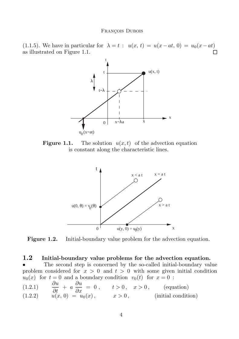
(1.1.5). We have in particular for λ = t : u(x, t) = u(x−at, 0) = u0(x−at)as illustrated on Figure 1.1.
t
xx
t
t−λ
λ
x−λa
u (x−at)0
u(x, t)
AAAA
0
Figure 1.1. The solution u(x, t) of the advection equationis constant along the characteristic lines.
x
t
u(y, 0) = u (y)0
x = a t
AAAAx < a t
u(0, θ) = v (θ)0
0
x > a tAAAAAAAAA
Figure 1.2. Initial-boundary value problem for the advection equation.
1.2 Initial-boundary value problems for the advection equation.• The second step is concerned by the so-called initial-boundary valueproblem considered for x > 0 and t > 0 with some given initial conditionu0(x) for t = 0 and a boundary condition v0(t) for x = 0 :
(1.2.1)∂u
∂t+ a
∂u
∂x= 0 , t > 0 , x > 0 , (equation)
(1.2.2) u(x, 0) = u0(x) , x > 0 , (initial condition)
An introduction to finite volumes for gas dynamics
(1.2.3) u(0, t) = v0(t) , t > 0 , (boundary condition).
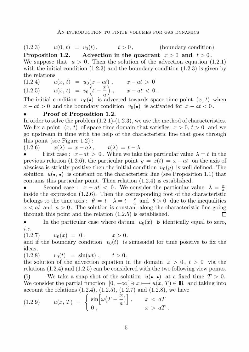
Proposition 1.2. Advection in the quadrant x > 0 and t > 0 .We suppose that a > 0 . Then the solution of the advection equation (1.2.1)with the initial condition (1.2.2) and the boundary condition (1.2.3) is given bythe relations(1.2.4) u(x, t) = u0(x− at) , x− at > 0
(1.2.5) u(x, t) = v0
(t − x
a
), x− at < 0 .
The initial condition u0(•) is advected towards space-time point (x, t) whenx− at > 0 and the boundary condition v0(•) is activated for x− at < 0 .
• Proof of Proposition 1.2.In order to solve the problem (1.2.1)-(1.2.3), we use the method of characteristics.We fix a point (x, t) of space-time domain that satisfies x > 0, t > 0 and wego upstream in time with the help of the characteristic line that goes throughthis point (see Figure 1.2) :(1.2.6) x(λ) = x− aλ , t(λ) = t− λ .• First case : x−at > 0 . When we take the particular value λ = t in theprevious relation (1.2.6), the particular point y = x(t) = x− at on the axis ofabscissa is strictly positive then the initial condition u0(y) is well defined. Thesolution u(•, •) is constant on the characteristic line (see Proposition 1.1) thatcontains this particular point. Then relation (1.2.4) is established.• Second case : x − at < 0 . We consider the particular value λ = x
ainside the expression (1.2.6). Then the corresponding foot of the characteristicbelongs to the time axis : θ = t−λ = t− x
a and θ > 0 due to the inequalitiesx < at and a > 0 . The solution is constant along the characteristic line goingthrough this point and the relation (1.2.5) is established.
• In the particular case where datum u0(x) is identically equal to zero,i.e.(1.2.7) u0(x) = 0 , x > 0 ,and if the boundary condition v0(t) is sinusoıdal for time positive to fix theideas,(1.2.8) v0(t) = sin(ωt) , t > 0 ,the solution of the advection equation in the domain x > 0 , t > 0 via therelations (1.2.4) and (1.2.5) can be considered with the two following view points.
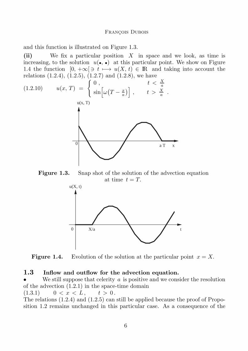
(i) We take a snap shot of the solution u(•, •) at a fixed time T > 0.We consider the partial function [0, +∞[ ∋ x 7−→ u(x, T ) ∈ IR and taking intoaccount the relations (1.2.4), (1.2.5), (1.2.7) and (1.2.8), we have
(1.2.9) u(x, T ) =
{sin[ω(T − x
a
)], x < aT
0 , x > aT .
Francois Dubois
and this function is illustrated on Figure 1.3.
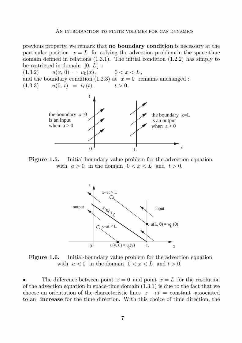
(ii) We fix a particular position X in space and we look, as time isincreasing, to the solution u(•, •) at this particular point. We show on Figure1.4 the function [0, +∞[∋ t 7−→ u(X, t) ∈ IR and taking into account therelations (1.2.4), (1.2.5), (1.2.7) and (1.2.8), we have
(1.2.10) u(x, T ) =
{0 , t < X
a
sin[ω(T − x
a
)], t > X
a .
x0
u(x, T)
a T
Figure 1.3. Snap shot of the solution of the advection equationat time t = T.
t0
u(X, t)
X/a
Figure 1.4. Evolution of the solution at the particular point x = X.
1.3 Inflow and outflow for the advection equation.• We still suppose that celerity a is positive and we consider the resolutionof the advection (1.2.1) in the space-time domain(1.3.1) 0 < x < L , t > 0 .The relations (1.2.4) and (1.2.5) can still be applied because the proof of Propo-sition 1.2 remains unchanged in this particular case. As a consequence of the
An introduction to finite volumes for gas dynamics
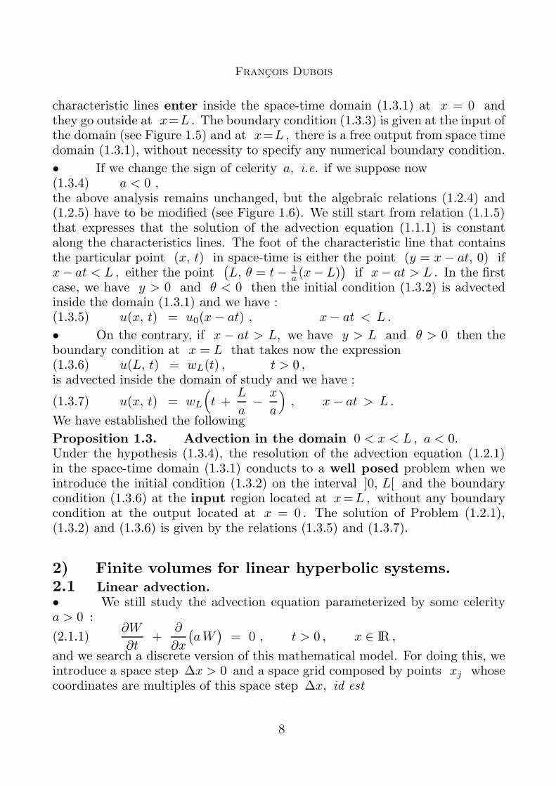
previous property, we remark that no boundary condition is necessary at theparticular position x = L for solving the advection problem in the space-timedomain defined in relations (1.3.1). The initial condition (1.2.2) has simply tobe restricted in domain ]0, L[ :(1.3.2) u(x, 0) = u0(x) , 0 < x < L ,and the boundary condition (1.2.3) at x = 0 remains unchanged :(1.3.3) u(0, t) = v0(t) , t > 0 .
x
t
0
the boundary x=0is an input when a > 0
L
the boundary x=Lis an output when a > 0
Figure 1.5. Initial-boundary value problem for the advection equationwith a > 0 in the domain 0 < x < L and t > 0.
x
t
u(y, 0) = u (y)0
x−at > L
u(L, θ) = w (θ)L
0 L
inputoutput
AAAA
AA
x−at = L
x−at < L
Figure 1.6. Initial-boundary value problem for the advection equationwith a < 0 in the domain 0 < x < L and t > 0.
• The difference between point x = 0 and point x = L for the resolutionof the advection equation in space-time domain (1.3.1) is due to the fact that wechoose an orientation of the characteristic lines x − at = constant associatedto an increase for the time direction. With this choice of time direction, the
Francois Dubois
characteristic lines enter inside the space-time domain (1.3.1) at x = 0 andthey go outside at x=L . The boundary condition (1.3.3) is given at the input ofthe domain (see Figure 1.5) and at x=L , there is a free output from space timedomain (1.3.1), without necessity to specify any numerical boundary condition.
• If we change the sign of celerity a, i.e. if we suppose now(1.3.4) a < 0 ,the above analysis remains unchanged, but the algebraic relations (1.2.4) and(1.2.5) have to be modified (see Figure 1.6). We still start from relation (1.1.5)that expresses that the solution of the advection equation (1.1.1) is constantalong the characteristics lines. The foot of the characteristic line that containsthe particular point (x, t) in space-time is either the point (y = x− at, 0) ifx− at < L , either the point
(L, θ = t− 1
a (x−L))
if x− at > L . In the firstcase, we have y > 0 and θ < 0 then the initial condition (1.3.2) is advectedinside the domain (1.3.1) and we have :(1.3.5) u(x, t) = u0(x− at) , x− at < L .
• On the contrary, if x − at > L, we have y > L and θ > 0 then theboundary condition at x = L that takes now the expression(1.3.6) u(L, t) = wL(t) , t > 0 ,is advected inside the domain of study and we have :
(1.3.7) u(x, t) = wL
(t +
L
a− x
a
), x− at > L .
We have established the following
Proposition 1.3. Advection in the domain 0 < x < L , a < 0.Under the hypothesis (1.3.4), the resolution of the advection equation (1.2.1)in the space-time domain (1.3.1) conducts to a well posed problem when weintroduce the initial condition (1.3.2) on the interval ]0, L[ and the boundarycondition (1.3.6) at the input region located at x=L , without any boundarycondition at the output located at x = 0 . The solution of Problem (1.2.1),(1.3.2) and (1.3.6) is given by the relations (1.3.5) and (1.3.7).
2) Finite volumes for linear hyperbolic systems.2.1 Linear advection.• We still study the advection equation parameterized by some celeritya > 0 :
(2.1.1)∂W
∂t+
∂
∂x
(aW
)= 0 , t > 0 , x ∈ IR ,
and we search a discrete version of this mathematical model. For doing this, weintroduce a space step ∆x > 0 and a space grid composed by points xj whosecoordinates are multiples of this space step ∆x, id est
An introduction to finite volumes for gas dynamics
(2.1.2) xj = j∆x , j ∈ ZZ .For a finite domain, ]0, L[ to fix the ideas, the above grid is limited to integervalues j such that
(2.1.3) 0 ≤ j ≤ J =L
∆xand the vertices (xj)0≤j≤J are usually used in the context of the finite differ-ence method. The intervals Kj+1/2 = ]xj , xj+1[ between two vertices can beconsidered as finite elements (or finite volumes in our study) and they cover theentire domain ]0, L[ :
(2.1.4) [0, L] =⋃
0≤j≤J−1
[xj , xj+1] ,
as proposed in the general context of meshes (see e.g. Ciarlet [Ci78]). Weintroduce also a time step ∆t > 0 and the discrete time values at integermultiples of the above quantum :(2.1.5) tn = n∆t , n ∈ IN .
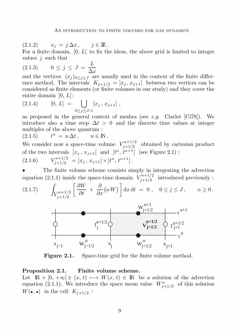
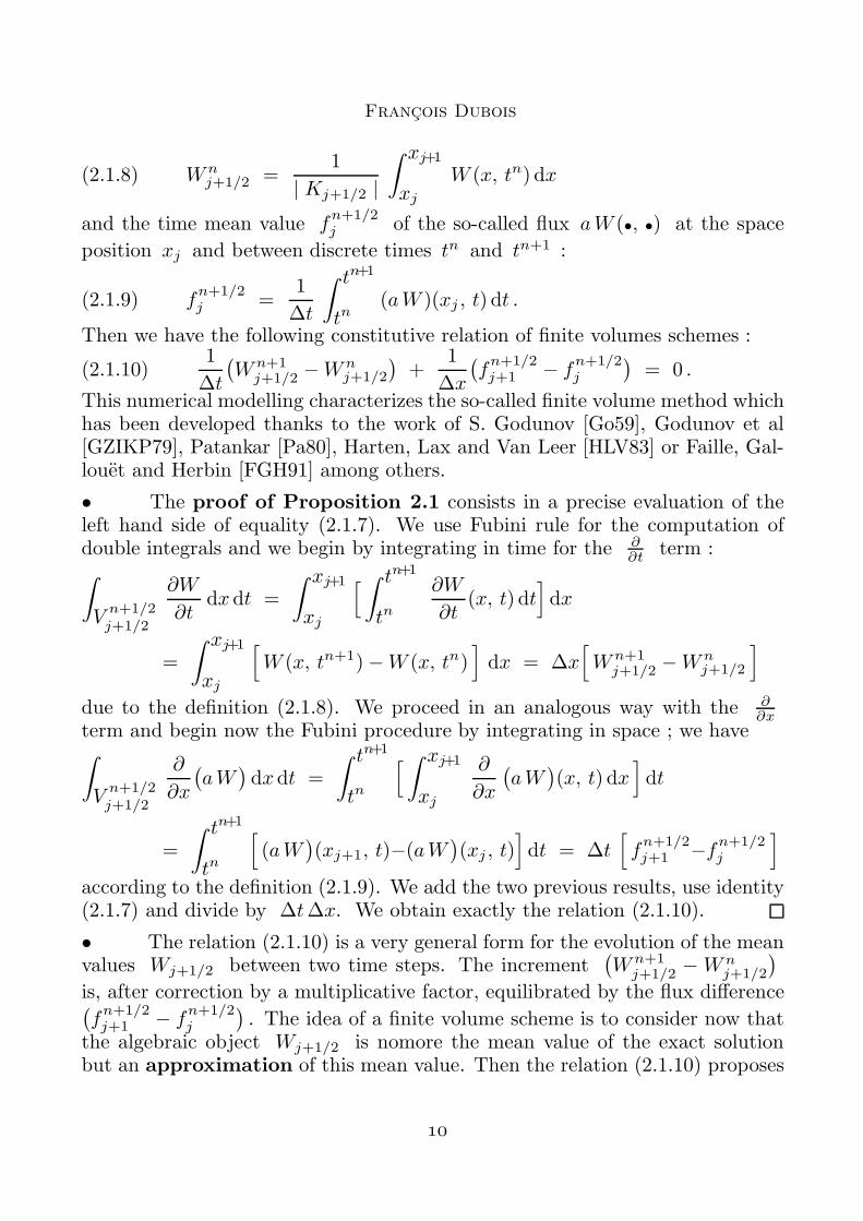
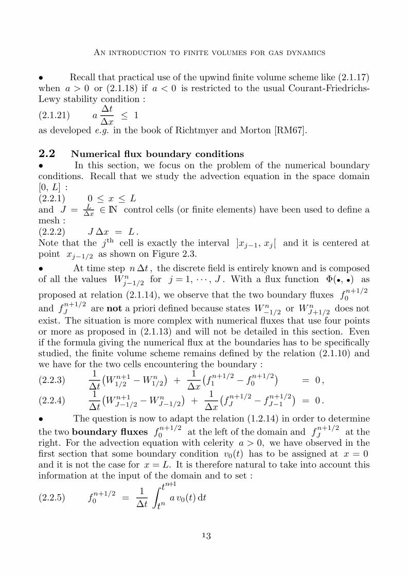
We consider now a space-time volume Vn+1/2j+1/2 obtained by cartesian product
of the two intervals ]xj , xj+1[ and ]tn, tn+1[ (see Figure 2.1) :
(2.1.6) Vn+1/2j+1/2 = ]xj , xj+1[× ]tn, tn+1[ .
• The finite volume scheme consists simply in integrating the advection
equation (2.1.1) inside the space-time domain Vn+1/2j+1/2 introduced previously :
(2.1.7)
∫
Vn+1/2j+1/2
[∂W
∂t+
∂
∂x
(aW
) ]dxdt = 0 , 0 ≤ j ≤ J , n ≥ 0 .
Wn+1j+1/2
Wnj+1/2
fn+1/2j f
n+1/2j+1
x j+1xj
tn+1
tn
Vn+1/2j+1/2
Wnj−1/2x j−1
Figure 2.1. Space-time grid for the finite volume method.
Proposition 2.1. Finite volume scheme.Let IR × [0, +∞[∋ (x, t) 7−→ W (x, t) ∈ IR be a solution of the advectionequation (2.1.1). We introduce the space mean value Wn
j+1/2 of this solution
W (•, •) in the cell Kj+1/2 :
Francois Dubois
(2.1.8) Wnj+1/2 =
1
| Kj+1/2 |
∫ xj+1
xjW (x, tn) dx
and the time mean value fn+1/2j of the so-called flux aW (•, •) at the space
position xj and between discrete times tn and tn+1 :
(2.1.9) fn+1/2j =
1
∆t
∫ tn+1
tn(aW )(xj , t) dt .
Then we have the following constitutive relation of finite volumes schemes :
(2.1.10)1
∆t
(Wn+1
j+1/2 −Wnj+1/2
)+
1
∆x
(fn+1/2j+1 − f
n+1/2j
)= 0 .
This numerical modelling characterizes the so-called finite volume method whichhas been developed thanks to the work of S. Godunov [Go59], Godunov et al[GZIKP79], Patankar [Pa80], Harten, Lax and Van Leer [HLV83] or Faille, Gal-louet and Herbin [FGH91] among others.
• The proof of Proposition 2.1 consists in a precise evaluation of theleft hand side of equality (2.1.7). We use Fubini rule for the computation ofdouble integrals and we begin by integrating in time for the ∂
∂t term :∫
Vn+1/2j+1/2
∂W
∂tdxdt =
∫ xj+1
xj
[ ∫ tn+1
tn∂W
∂t(x, t) dt
]dx
=
∫ xj+1
xj
[W (x, tn+1)−W (x, tn)
]dx = ∆x
[Wn+1
j+1/2 −Wnj+1/2
]
due to the definition (2.1.8). We proceed in an analogous way with the ∂∂x
term and begin now the Fubini procedure by integrating in space ; we have∫
Vn+1/2j+1/2
∂
∂x
(aW
)dxdt =
∫ tn+1
tn
[ ∫ xj+1
xj
∂
∂x
(aW
)(x, t) dx
]dt
=
∫ tn+1
tn
[(aW
)(xj+1, t)−(aW
)(xj , t)
]dt = ∆t
[fn+1/2j+1 −fn+1/2
j
]
according to the definition (2.1.9). We add the two previous results, use identity(2.1.7) and divide by ∆t∆x. We obtain exactly the relation (2.1.10).
• The relation (2.1.10) is a very general form for the evolution of the meanvalues Wj+1/2 between two time steps. The increment
(Wn+1
j+1/2 −Wnj+1/2
)
is, after correction by a multiplicative factor, equilibrated by the flux difference(fn+1/2j+1 − f
n+1/2j
). The idea of a finite volume scheme is to consider now that
the algebraic object Wj+1/2 is nomore the mean value of the exact solutionbut an approximation of this mean value. Then the relation (2.1.10) proposes
An introduction to finite volumes for gas dynamics
a numerical scheme for the discrete evolution of the approximated mean valuesWj+1/2 , j = 0, · · · , J−1. Nevertheless, the numerical scheme is not entirelydefined by the relation (2.1.10). Starting from mean values at the initial timestep, i.e.
(2.1.11) W 0j+1/2 =
1
∆x
∫ xj+1
xjW0(x) dx , j = 0, · · · , J−1 ,
we are able to increment the time step with relation (2.1.10) only if all the fluxes
fn+1/2j , j = 0, · · · , J have been a priori first determined as a functional of theprevious values. In a very general way, we say that the finite volume scheme
(2.1.10) is an explicit scheme if each flux fn+1/2j is a given function Ψj of
the mean values(Wn
k+1/2
)k=1,···, J−1
at the preceding time step number n :
(2.1.12) fn+1/2j = Ψj
({Wn
k+1/2, k = 0, · · · , J−1}), j = 0, · · · , J−1 .
The function Ψj is called the local numerical flux function at point xj and,joined with the evolution equation (2.1.10), its choice determines the numericalscheme.
• A natural hypothesis claims that we have translation invariance forthe evaluation of the flux if we move the discrete data in the same way ; in otherwords, the numerical flux function Ψj only depends on the p first neighborsof the interface xj . Then the explicit numerical flux is a given function Φ ofthe p first neighbors and we have :
(2.1.13) fn+1/2j = Φ
(Wn
j+1/2−p, · · · , Wnj−1/2, W
nj+1/2, · · · , Wn
j+1/2+p−1
).
A very important particular case is one of a two-point scheme for the evaluationof the numerical flux. We have in this particular case :
(2.1.14) fn+1/2j = Φ
(Wn
j−1/2, Wnj+1/2
).
With this particular choice, the numerical scheme for incrementing in time ofthe mean values takes the form :
(2.1.15)
1
∆t
(Wn+1
j+1/2 −Wnj+1/2
)+
+1
∆x
(Φ(Wn
j+1/2, Wnj+3/2
)− Φ
(Wn
j−1/2, Wnj+1/2
))= 0 .
It is also a three-point finite difference scheme. The finite volume scheme (2.1.10)(2.1.13) is said to be consistent with the advection equation (2.1.1) when thenumerical flux function Φ satisfies the condition(2.1.16) Φ
(W, · · · , W, W, · · · , W
)= aW , ∀W ∈ IR .
• The crucial question is how to choose a numerical finite volume scheme.The simplest choice consists in a two point explicit scheme such that the fi-nite difference scheme is identical to the upstream-centered scheme (see e.g.Richtmyer-Morton [RM67]). It takes the following expressions :
Francois Dubois
(2.1.17)1
∆t
(Wn+1
j+1/2 −Wnj+1/2
)+ a
(Wn
j+1/2 −Wnj−1/2
)= 0 , a > 0
(2.1.18)1
∆t
(Wn+1
j+1/2 −Wnj+1/2
)+ a
(Wn
j+3/2 −Wnj+1/2
)= 0 , a < 0 .
The corresponding flux function is called the first order upstream-centeredflux, is simply given by the following relations :
(2.1.19) Φ(Wl, Wr) =
{aWl , a > 0aWr , a < 0 .
When this flux function acts at a given point xj of the mesh, we have :
(2.1.20) fn+1/2j = Φ
(Wn
j−1/2, Wnj+1/2
)=
{aWn
j−1/2 , a > 0
aWnj+1/2 , a < 0 .
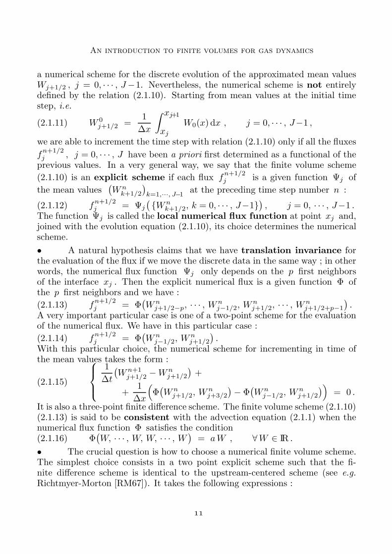
If a > 0, the exact solution of the advection equation propagates the informationfrom the left to the right ; the flux at the interface xj is issued from the cellat the left of the interface and this cell at the number j−1/2 . If a < 0, thepropagation of the information with the advection equation is from right to left ;the interface flux at the abscissa xj is due to the control volume on the right,i.e. with number j+1/2 as depicted on Figure 2.2.
xj
Wn
j−1/2 a > 0
Wnj+1/2
a < 0
Figure 2.2. Upwinding of the information for the advection equation.
0x = 0
1x ...
j−1x
jx ...
J−1x
Jx = L
W1/2f0 f
J
WJ−1/2
Wj−1/2
j−1/2x
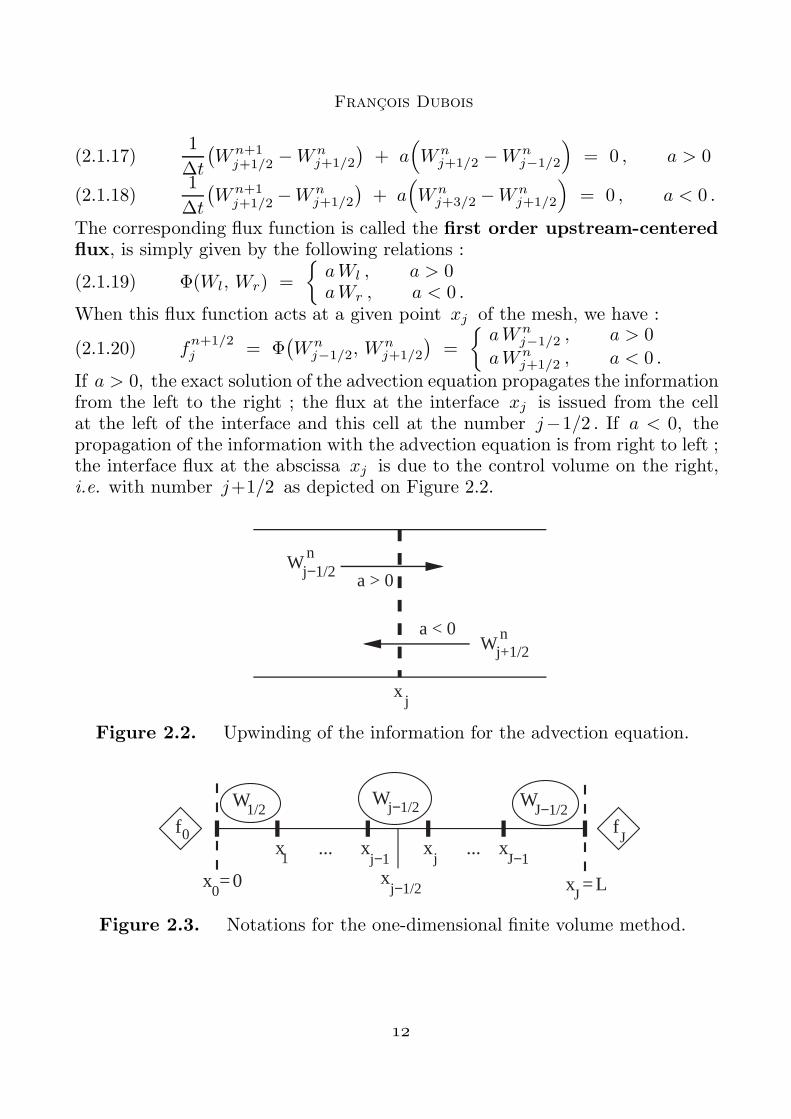
Figure 2.3. Notations for the one-dimensional finite volume method.
An introduction to finite volumes for gas dynamics
• Recall that practical use of the upwind finite volume scheme like (2.1.17)when a > 0 or (2.1.18) if a < 0 is restricted to the usual Courant-Friedrichs-Lewy stability condition :
(2.1.21) a∆t
∆x≤ 1
as developed e.g. in the book of Richtmyer and Morton [RM67].
2.2 Numerical flux boundary conditions• In this section, we focus on the problem of the numerical boundaryconditions. Recall that we study the advection equation in the space domain[0, L] :(2.2.1) 0 ≤ x ≤ Land J = L
∆x ∈ IN control cells (or finite elements) have been used to define amesh :(2.2.2) J ∆x = L .Note that the jth cell is exactly the interval ]xj−1, xj [ and it is centered atpoint xj−1/2 as shown on Figure 2.3.
• At time step n∆t , the discrete field is entirely known and is composedof all the values Wn
j−1/2 for j = 1, · · · , J . With a flux function Φ(•, •) as
proposed at relation (2.1.14), we observe that the two boundary fluxes fn+1/20
and fn+1/2J are not a priori defined because states Wn
−1/2 or WnJ+1/2 does not
exist. The situation is more complex with numerical fluxes that use four pointsor more as proposed in (2.1.13) and will not be detailed in this section. Evenif the formula giving the numerical flux at the boundaries has to be specificallystudied, the finite volume scheme remains defined by the relation (2.1.10) andwe have for the two cells encountering the boundary :
(2.2.3)1
∆t
(Wn+1
1/2 −Wn1/2
)+
1
∆x
(fn+1/21 − f
n+1/20
)= 0 ,
(2.2.4)1
∆t
(Wn+1
J−1/2 −WnJ−1/2
)+
1
∆x
(fn+1/2J − f
n+1/2J−1
)= 0 .
• The question is now to adapt the relation (1.2.14) in order to determine
the two boundary fluxes fn+1/20 at the left of the domain and f
n+1/2J at the
right. For the advection equation with celerity a > 0, we have observed in thefirst section that some boundary condition v0(t) has to be assigned at x = 0and it is not the case for x = L. It is therefore natural to take into account thisinformation at the input of the domain and to set :
(2.2.5) fn+1/20 =
1
∆t
∫ tn+1
tna v0(t) dt
Francois Dubois
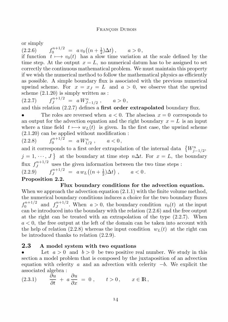
or simply
(2.2.6) fn+1/20 = a v0
((n+ 1
2 )∆t), a > 0 ,
if function t 7−→ v0(t) has a slow time variation at the scale defined by thetime step. At the output x = L, no numerical datum has to be assigned to setcorrectly the continuous mathematical problem. We must maintain this propertyif we wish the numerical method to follow the mathematical physics as efficientlyas possible. A simple boundary flux is associated with the previous numericalupwind scheme. For x = xJ = L and a > 0, we observe that the upwindscheme (2.1.20) is simply written as :
(2.2.7) fn+1/2J = aWn
J−1/2 , a > 0 ,
and this relation (2.2.7) defines a first order extrapolated boundary flux.
• The roles are reversed when a < 0. The abscissa x = 0 corresponds toan output for the advection equation and the right boundary x = L is an inputwhere a time field t 7−→ wL(t) is given. In the first case, the upwind scheme(2.1.20) can be applied without modification :
(2.2.8) fn+1/20 = aWn
1/2 , a < 0 ,
and it corresponds to a first order extrapolation of the internal data{Wn
j−1/2,
j = 1, · · · , J}
at the boundary at time step n∆t. For x = L, the boundary
flux fn+1/2J uses the given information between the two time steps :
(2.2.9) fn+1/2J = awL
((n+ 1
2 )∆t), a < 0 .
Proposition 2.2.Flux boundary conditions for the advection equation.
When we approach the advection equation (2.1.1) with the finite volume method,the numerical boundary conditions induces a choice for the two boundary fluxes
fn+1/20 and f
n+1/2J . When a > 0, the boundary condition v0(t) at the input
can be introduced into the boundary with the relation (2.2.6) and the free outputat the right can be treated with an extrapolation of the type (2.2.7). Whena < 0, the free output at the left of the domain can be taken into account withthe help of relation (2.2.8) whereas the input condition wL(t) at the right canbe introduced thanks to relation (2.2.9).
2.3 A model system with two equations• Let a > 0 and b > 0 be two positive real number. We study in thissection a model problem that is composed by the juxtaposition of an advectionequation with celerity a and an advection with celerity −b. We explicit theassociated algebra :
(2.3.1)∂u
∂t+ a
∂u
∂x= 0 , t > 0 , x ∈ IR ,
An introduction to finite volumes for gas dynamics
(2.3.2)∂v
∂t− b
∂v
∂x= 0 , t > 0 , x ∈ IR .
We associate the two equations (2.3.1) and (2.3.2) and consider a unique problemwith a vector field as unknown. We set :
(2.3.3) ϕ =
(uv
)
and the set of equations (2.3.1)-(2.3.2) can naturally be written as a system :
(2.3.4)∂ϕ
∂t+
(a 00 −b
)∂ϕ
∂x= 0 .
By introducing the flux function F (ϕ) according to the relation
(2.3.5) F (ϕ) =
(au−b v
)
the system (2.3.4) takes the general conservative form :
(2.3.6)∂ϕ
∂t+
∂
∂x
(F (ϕ)
)= 0 .
• The approximation of system (2.3.6) with a grid parameterized by aspace step ∆x and a time step ∆t is conducted exactly as in the case of theadvection equation. The following property is a straightforward generalizationof Proposition 2.1. We left the proof to the reader.
Proposition 2.3. Finite volume scheme.Let IR × [0, +∞[ ∋ (x, t) 7−→ ϕ(x, t) ∈ IR × IR be a solution of the linearconservation law (2.3.6). We define the space mean value ϕn
j+1/2 of this solution
ϕ(•, •) in the cell Kj+1/2 :
(2.3.7) ϕnj+1/2 =
1
| Kj+1/2 |
∫ xj+1
xjϕ(x, tn) dx
and the time mean value fn+1/2j of the flux function introduced in (2.3.5) at
the space position xj between discrete times tn and tn+1 :
(2.3.8) fn+1/2j =
1
∆t
∫ tn+1
tnF(ϕ(xj , t)
)dt .
We have the following relation that characterizes the finite volumes schemes :
(2.3.9)1
∆t
(ϕn+1j+1/2 − ϕn
j+1/2
)+
1
∆x
(fn+1/2j+1 − f
n+1/2j
)= 0 .
• We have now to propose a precise numerical flux function analogousto the relation (2.1.12) to transform the conservation property (2.3.9) into afinite volume numerical scheme able to propagate the discrete values ϕn
j+1/2
up to the discrete time tn+1. For internal interfaces xj , j = 1, · · · , J−1 , it isnatural to apply the upwinding scheme (2.1.20) with a left upwinding for the first
Francois Dubois
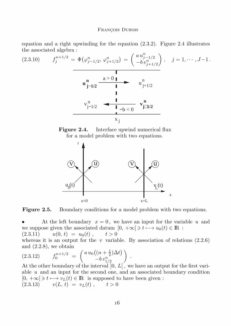
equation and a right upwinding for the equation (2.3.2). Figure 2.4 illustratesthe associated algebra :
(2.3.10) fn+1/2j = Φ
(ϕnj−1/2, ϕ
nj+1/2
)=
(aunj−1/2
−b vnj+1/2
), j = 1, · · · , J−1 .
unj+1/2
v nj−1/2
x j
−b < 0
a > 0u n
j−1/2
v nj+1/2
Figure 2.4. Interface upwind numerical fluxfor a model problem with two equations.
t
x
x=Lx=0
u (t)0 v (t)
L
uv v u
Figure 2.5. Boundary conditions for a model problem with two equations.
• At the left boundary x = 0 , we have an input for the variable u andwe suppose given the associated datum [0, +∞[∋ t 7−→ u0(t) ∈ IR :(2.3.11) u(0, t) = u0(t) , t > 0whereas it is an output for the v variable. By association of relations (2.2.6)and (2.2.8), we obtain
(2.3.12) fn+1/20 =
(au0
((n+ 1
2 )∆t)
−b vn1/2
).
At the other boundary of the interval ]0, L[ , we have an output for the first vari-able u and an input for the second one, and an associated boundary condition[0, +∞[∋ t 7−→ vL(t) ∈ IR is supposed to have been given :(2.3.13) v(L, t) = vL(t) , t > 0
An introduction to finite volumes for gas dynamics
as illustrated on Figure 2.5. The numerical flux at the right is evaluated byassociation of the relations (2.2.7) and (2.2.9) :
(2.3.14) fn+1/2L =
(aunJ−1/2
−b vL((n+ 1
2 )∆t)).
2.4 Unidimensional linear acoustics• We consider a gas in a pipe of uniform section at normal conditionsof temperature and pressure. The reference density is denoted by ρ0 and thereference pressure is named p0. The sound celerity c0 of this gas satisfies therelation
(2.4.1) c0 =
√γp0ρ0
with γ = 1.4 as proved e.g. in the book of Landau and Lifchitz [LL54]. Asound wave is a small perturbation of this reference state. The differences ofdensity, pressure and velocity fields are denoted respectively by ρ, p and u. Thehypothesis of a small perturbation implies that the entropy of the reference stateis maintained for all the time evolution and in consequence, it is easy to establishthe following relation between the perturbations of density and pressure :(2.4.2) p = c20 ρ .
• The conservation of mass leads to a first order linear conservation law :
(2.4.3)∂ρ
∂t+ ρ0
∂u
∂x= 0
and the conservation of momentum links the time evolution of velocity with thespatial gradient of pressure :
(2.4.4) ρ0∂u
∂t+
∂p
∂x= 0 .
We introduce the vector W =
(pu
)of unknowns. Then the equations (2.4.3)
and (2.4.4) can be written as a linear hyperbolic system of conservation laws :
(2.4.5)∂W
∂t+ A
∂W
∂x= 0
with
(2.4.6) A =
(0 ρ0 c
20
1ρ0
0
).
• When we consider the eigenvalues and eigenvectors of matrix A, it isnatural to introduce the characteristic variables defined respectively by(2.4.7) ϕ+ = p + ρ0 c0 u(2.4.8) ϕ− = p − ρ0 c0 uand the quantity ρ0 c0 is named the acoustic impedance. We have from therelations (2.4.3) and (2.4.4) :
Francois Dubois
∂ϕ+
∂t+ c0
∂ϕ+
∂x=(∂p∂t
+ ρ0 c0∂u
∂t
)+(c0∂p
∂x+ ρ0 c
20
∂u
∂x
)
= c20
(∂ρ∂t
+ ρ0∂u
∂x
)+ c0
(ρ0∂u
∂t+
∂p
∂x
)= 0 ,
∂ϕ−
∂t− c0
∂ϕ−
∂x=(∂p∂t
− ρ0 c0∂u
∂t
)− c0
(∂p∂x
− ρ0 c0∂u
∂x
)
= c20
(∂ρ∂t
+ ρ0∂u
∂x
)− c0
(ρ0∂u
∂t+
∂p
∂x
)= 0 ,
and we recover a system of the type (2.3.4) studied previously :
(2.4.9)∂
∂t
(ϕ−
ϕ+
)+
(−c0 00 c0
)∂
∂t
(ϕ−
ϕ+
)= 0 .
• A typically physical problem is the following : a given acoustic pressurewave [0, +∞[ ∋ t 7−→ Π(t) > 0 is injected at the left x = 0 of the pipe andthe waves go away freely at the right boundary x=L . At t = 0, the velocityand pressure of the fluid are given :(2.4.10) u(x, 0) = u0(x) , 0 < x < L(2.4.11) p(x, 0) = p0(x) , 0 < x < L .From a mathematical viewpoint, the boundary conditions have to respect thedynamics of this system of acoustic equations written in diagonal form (2.4.9) :the variable ϕ+ must be given at x= 0 and the variable ϕ− at the abscissax=L. From (2.4.7) and (2.4.8), we determine the pressure as a function of thetwo characteristics variables ϕ+ and ϕ− :
(2.4.12) p =1
2
(ϕ+ + ϕ−
)
and if the pressure is imposed at x = 0, the relation (2.4.12) can be writtenunder the form :(2.4.13) ϕ+(0, t) = −ϕ−(0, t) + 2Π(t) , x = 0 , t > 0 ,that makes in evidence a reflection operator : the input variable ϕ+ is a givenaffine function of the output variable ϕ− . At the other boundary x=L , thenotion of free output expresses that the waves that go outside of the domainof study have no reflection at the boundary. When x = L , the characteristicvariable ϕ+ is going outside and there is no boundary condition for this variable.We have to express also that this wave has no influence on the characteristic ϕ−
that wish to go inside the domain ]0, L[. In other terms, the input value ϕ− isindependent of the variable ϕ+ and also of time. We have in consequence
(2.4.14)∂
∂tϕ−(L, t) = 0 .
We have established
An introduction to finite volumes for gas dynamics
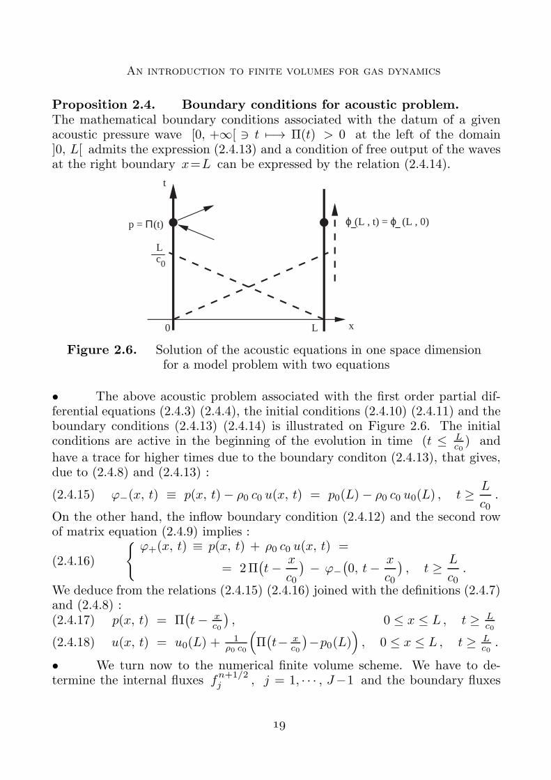
Proposition 2.4. Boundary conditions for acoustic problem.The mathematical boundary conditions associated with the datum of a givenacoustic pressure wave [0, +∞[ ∋ t 7−→ Π(t) > 0 at the left of the domain]0, L[ admits the expression (2.4.13) and a condition of free output of the wavesat the right boundary x=L can be expressed by the relation (2.4.14).
0 L x
Lc0
p = Π(t)
t
ϕ (L , t) = ϕ (L , 0)− −
Figure 2.6. Solution of the acoustic equations in one space dimensionfor a model problem with two equations
• The above acoustic problem associated with the first order partial dif-ferential equations (2.4.3) (2.4.4), the initial conditions (2.4.10) (2.4.11) and theboundary conditions (2.4.13) (2.4.14) is illustrated on Figure 2.6. The initialconditions are active in the beginning of the evolution in time (t ≤ L
c0) and
have a trace for higher times due to the boundary conditon (2.4.13), that gives,due to (2.4.8) and (2.4.13) :
(2.4.15) ϕ−(x, t) ≡ p(x, t)− ρ0 c0 u(x, t) = p0(L)− ρ0 c0 u0(L) , t ≥ L
c0.
On the other hand, the inflow boundary condition (2.4.12) and the second rowof matrix equation (2.4.9) implies :
(2.4.16)
{ϕ+(x, t) ≡ p(x, t) + ρ0 c0 u(x, t) =
= 2Π(t− x
c0
)− ϕ−
(0, t− x
c0
), t ≥ L
c0.
We deduce from the relations (2.4.15) (2.4.16) joined with the definitions (2.4.7)and (2.4.8) :(2.4.17) p(x, t) = Π
(t− x
c0
), 0 ≤ x ≤ L , t ≥ L
c0
(2.4.18) u(x, t) = u0(L) +1
ρ0 c0
(Π(t− x
c0
)−p0(L)
), 0 ≤ x ≤ L , t ≥ L
c0.
• We turn now to the numerical finite volume scheme. We have to de-termine the internal fluxes f
n+1/2j , j = 1, · · · , J−1 and the boundary fluxes
Francois Dubois
fn+1/20 and f
n+1/2J . Recall first that the physical flux F (W ) function for the
acoustic equation (2.4.5) is equal to
(2.4.19) F (W ) =
(ρ0 c
20 u
1ρ0
p
)with W =
(pu
).
Proposition 2.5. Upwind scheme for computational acoustics.The extension of the upwind finite volume scheme (2.3.10), (2.3.12) and (2.3.14)is determined by the following relations :
(2.4.20) fn+1/2j =
(ρ0 c2
0
2
(unj−1/2 + unj+1/2
)− c0
2
(pnj+1/2 − pnj−1/2
)1
2 ρ0
(pnj−1/2 + pnj+1/2
)− c0
2
(unj+1/2 − unj−1/2
))
for the internal fluxes, i.e. for indexes j that satisfy 1 ≤ j ≤ J−1 . The twoboundary fluxes follow the following relations :
(2.4.21) fn+1/20 =
(ρ0 c
20 u
n1/2 + c0
(Π((n+ 1
2)∆t
)− pn1/2
)
1ρ0
Π((n+ 1
2 )∆t)
)
(2.4.22) fn+1/2J =
(ρ0 c2
0
2
(unJ−1/2 + u0J−1/2
)− c0
2
(p0J−1/2 − pnJ−1/2
)1
2 ρ0
(pnJ−1/2 + p0J−1/2
)− c0
2
(u0J−1/2 − unJ−1/2
)).
• The internal fluxes are determined with the scheme (2.3.10) applied withthe diagonal form of relation (2.4.9). We have
(2.4.23) ϕn+1/2+, j = ϕn
+, j−1/2 ≡ pnj−1/2 + ρ0 c0 unj−1/2
(2.4.24) ϕn+1/2−, j = ϕn
−, j+1/2 ≡ pnj+1/2 − ρ0 c0 unj+1/2
then the relation (2.4.20) is established.The left boundary flux uses the extension of relation (2.3.12). We first determinethe characteristic variables on the left boundary according to relation (2.4.13)
(2.4.25) ϕn+1/2+, 0 = 2Π
((n+
1
2)∆t
)− ϕ
n+1/2−, 0
and use a first order extrapolation of the outgoing characteristic variable :
(2.4.26) ϕn+1/2−, 0 = ϕn
−, 1/2 ≡ pn1/2 − ρ0 c0 un1/2 .
Then we solve the system (2.4.25) (2.4.26) and find finally the relation (2.4.21).The process is analogous for the right boundary. The input datum is imposedaccording to the relation (2.4.14) :
(2.4.27) ϕn+1/2−, J = ϕ0
−, J ≡ p0(L)− ρ0 c0 u0(L) ≈ p0J−1/2 − ρ0 c0 u0J−1/2
and the output characteristic variable is extrapolated from the interior of thedomain :(2.4.28) ϕ
n+1/2+, J = ϕn
+, J−1/2 ≡ pnJ−1/2 + ρ0 c0 unJ−1/2 .
The relation (2.4.22) follows after two steps of elementary algebra.
An introduction to finite volumes for gas dynamics
• We remark that both relations (2.4.20) and (2.4.22) are identical, exceptthat the boundary state W0(L) ≈W 0
J−1/2 has replaced the right state Wnj+1/2 .
Moreover the flux boundary condition (2.4.21) that involves the pressure is anatural discretization of the exact characteristic solution (2.4.17) (2.4.18) atx=0 .
2.5 Characteristic variables.• We suppose now to fix the ideas that the unknown vector W (•, •)(2.5.1) [0, L]× [0, +∞[ ∋ (x, t) 7−→W (x, t) ∈ IR3
has three real components w1, w2 and w3. We suppose also that the functionW (•, •) is solution of a conservation law of the type
(2.5.2)∂W
∂t+
∂
∂xF (W ) = 0
where the flux F (W ) is a linear function of vector W :(2.5.3) F (W ) = A •Wand A is a 3 by 3 diagonalizable real matrix.
• We first detail the fact that matrix A is a diagonalizable matrix. Thereexists three non null real vectors r1 , r2 , r3 and three real scalars λ1 , λ2 ,λ3 in such a way that(2.5.4) A • rj = λj rj , j = 1, 2, 3.¿From a matricial viewpoint, we denote by Rk j the k0 component of theeigenvector rj , i.e.
(2.5.5) rj =
R1 j
R2 j
R3 j
≡
(rj)1(
rj)2(
rj)3
and we introduce the 3 by 3 matrix R composed by the scalars Rk j . The vectorrj is the k0 column of matrix R. The relation (2.5.4) can also be written as(2.5.6) A •R = R •Λ ,and Λ is the diagonal matrix whose diagonal terms are equal to the eigenvaluesλj :
(2.5.7) Λ =
λ1 0 00 λ2 00 0 λ3
.
• We consider now two distinct bases for linear space IR3 : on one handthe canonical basis
(ej)j=1, 2, 3
defined by
(2.5.8) e1 =
100
, e2 =
010
, e3 =
001
Francois Dubois
where the vector W admits the natural decomposition introduced above :
(2.5.9) W =∑k=3
k=1 wk ek ,
and on the other hand the basis of IR3 composed by the eigenvectors (rj)j=1, 2, 3.In the latter, the vector W can be decomposed with a formula of the type
(2.5.10) W =∑j=3
j=1 ϕj rj
and the scalar ϕj define the characteristic variables associated with thesystem (2.5.2) (2.5.3). The link between the relations (2.5.9) and (2.5.10) isclassical : we consider the components Rk j of vector rj inside the canonicalbasis and we get from the relation (2.5.5) :
(2.5.11) wk =∑j=3
j=1 ϕj Rk j .
Then the relation (2.5.11) can be re-written under a matricial form :
(2.5.12) W = R •ϕ .
• The relation (2.5.12) proposes to change the unknown function, i.e.to replace the research of W (x, t) ∈ IR3 by the equivalent research of thecharacteristic vector ϕ(x, t) ∈ IR3 and defined by :
(2.5.13) ϕ = R−1•W .
Proposition 2.6. Characteristic variables satisfy advection equations.
The vector [0, L]×[0, +∞[ ∋ (x, t) 7−→ ϕ(x, t) ∈ IR3 of characteristic variablessatisfy the matrix equation
(2.5.14)∂ϕ
∂t+ Λ •
∂ϕ
∂x= 0
that takes also the equivalent scalar form :
(2.5.15)∂ϕj
∂t+ λj
∂ϕj
∂x= 0 , j = 1, 2, 3 .
• We have from (2.5.2), (2.5.3), (2.5.6) and (2.5.12) :
∂W
∂t+ A
∂W
∂x= R •
∂ϕ
∂t+ A •R •
∂ϕ
∂x= R •
(∂ϕ
∂t+ R−1
•A •R •∂ϕ
∂x
)
= R •
(∂ϕ
∂t+ Λ •
∂ϕ
∂x
)= 0 ,
and since the matrix R is invertible, we deduce from the previous calculus therelation (2.5.14). The relation (2.5.15) is an immediate consequence of (2.5.14)and (2.5.7).
An introduction to finite volumes for gas dynamics
λ2
λ3
λ1
λ3
λ2λ
1
x = 0 x = L
t
x
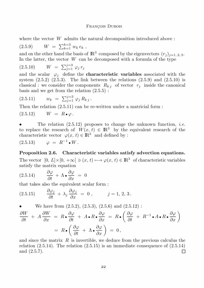
Figure 2.7. Linear hyperbolic system with three equationsand eigenvalues satisfying λ1 < 0 < λ2 < λ3.
• To fix the ideas, we suppose that the eigenvalues λj of matrix Aare distinct, enumerated with an increasing order and with distinct signs asillustrated on Figure 2.7 :
(2.5.16) λ1 < 0 < λ2 < λ3 .
The propagation of the first variable ϕ1 goes from right to left (because λ1 < 0 )with celerity |λ1 |, the second characteristic variable ϕ2 from left to right withcelerity λ2 and the same property holds for variable ϕ3 with eigenvalue λ3.
• A set of well posed boundary conditions is a consequence of the diagonalform (2.5.15) of the equations and of the particular choice (2.5.16) for the signs.The directions associated with eigenvalues λ2 and λ3 are ingoing at x=0 andwe have to give some boundary condition for ϕ2 and ϕ3 at this point :
(2.5.17) ϕ2(x=0, t) = β0(t)
(2.5.18) ϕ3(x=0, t) = γ0(t) .
The direction associated with the eigenvalue λ1 is ingoing at the abscisssa x=L,and this condition imposes to have some datum concerning ϕ1 at this particularpoint :
(2.5.19) ϕ1(x=L, t) = αL(t) .
The previous boundary conditions (2.5.17) to (2.5.19) define a well posed prob-lem. Nevertheless, the introduction of physically relevant boundary conditions(as a pressure condition as seen in the previous section) requires a more generalformulation of the boundary condition. In the linear case, the stability studydeveloped by Kreiss [Kr70] shows that the ingoing characteristic can be an affinefunction of the outgoing characteristic through a reflection operator at theboundary. We can explicit the former with the above example.
Francois Dubois
λ3
λ2
λ1
x = 0
t
x
p
q
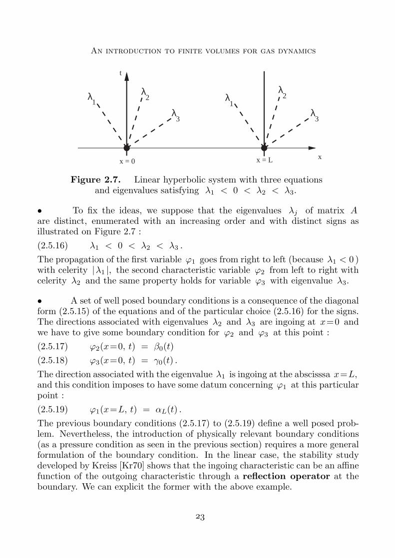
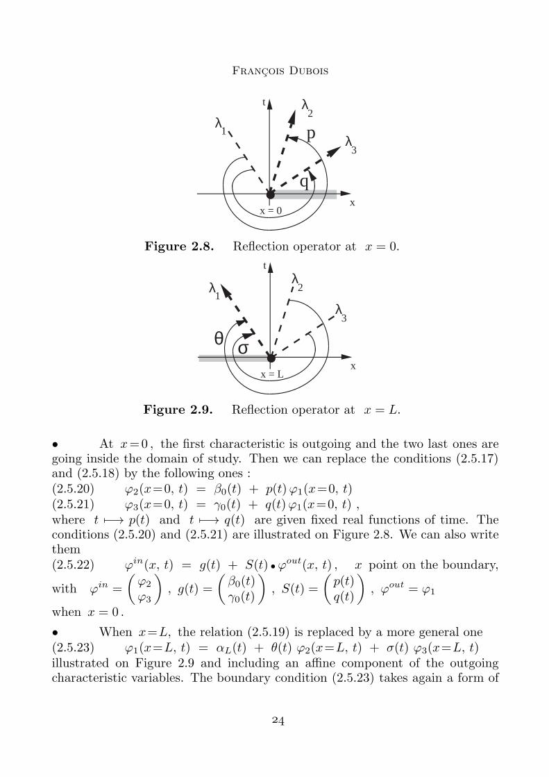
Figure 2.8. Reflection operator at x = 0.
λ3
λ2λ
1
x = L
t
x
θ σ
Figure 2.9. Reflection operator at x = L.
• At x=0 , the first characteristic is outgoing and the two last ones aregoing inside the domain of study. Then we can replace the conditions (2.5.17)and (2.5.18) by the following ones :(2.5.20) ϕ2(x=0, t) = β0(t) + p(t)ϕ1(x=0, t)(2.5.21) ϕ3(x=0, t) = γ0(t) + q(t)ϕ1(x=0, t) ,where t 7−→ p(t) and t 7−→ q(t) are given fixed real functions of time. Theconditions (2.5.20) and (2.5.21) are illustrated on Figure 2.8. We can also writethem(2.5.22) ϕin(x, t) = g(t) + S(t) •ϕout(x, t) , x point on the boundary,
with ϕin =
(ϕ2
ϕ3
), g(t) =
(β0(t)γ0(t)
), S(t) =
(p(t)q(t)
), ϕout = ϕ1
when x = 0 .
• When x=L, the relation (2.5.19) is replaced by a more general one(2.5.23) ϕ1(x=L, t) = αL(t) + θ(t) ϕ2(x=L, t) + σ(t) ϕ3(x=L, t)illustrated on Figure 2.9 and including an affine component of the outgoingcharacteristic variables. The boundary condition (2.5.23) takes again a form of
An introduction to finite volumes for gas dynamics
the type (2.5.22) with this time the following relations : ϕin = ϕ1 , g(t) =
αL(t) , S(t) =(θ(t) σ(t)
), ϕout =
(ϕ2
ϕ3
)when x=L .
2.6 A family of model systems with three equations• We still study a 3 by 3 linear hyperbolic system of the type (2.5.2)(2.5.3) with the condition (2.5.16) to fix a particular example. We suggest in
this section to explicit a way for evaluation of the numerical flux fn+1/2j that
is the key point for the discrete evolution in time of the mean values Wj+1/2 :
(2.6.1)1
∆t
(Wn+1
j+1/2 − Wnj+1/2
)+
1
∆x
(fn+1/2j+1 − f
n+1/2j
)= 0 .
The internal fluxes(fn+1/2j
)j=1,···, J−1
are evaluated with the help of a two-
point numerical flux function Φ(•, •) :
(2.6.2) fn+1/2j = Φ(Wn
j−1/2, Wnj+1/2)
and the boundary fluxes fn+1/20 and f
n+1/2J are detailed in a forthcoming
sub-section.t
Wleft
Wright
x
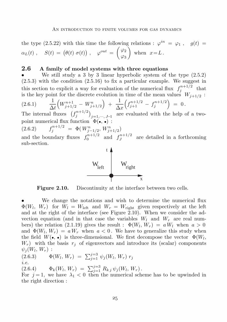
Figure 2.10. Discontinuity at the interface between two cells.
• We change the notations and wish to determine the numerical fluxΦ(Wl, Wr) for Wl = Wleft and Wr = Wright given respectively at the leftand at the right of the interface (see Figure 2.10). When we consider the ad-vection equation (and in that case the variables Wl and Wr are real num-bers) the relation (2.1.19) gives the result : Φ(Wl, Wr) = aWl when a > 0and Φ(Wl, Wr) = aWr when a < 0 . We have to generalize this study whenthe field W (•, •) is three-dimensional. We first decompose the vector Φ(Wl,Wr) with the basis rj of eigenvectors and introduce its (scalar) componentsψj(Wl, Wr) :
(2.6.3) Φ(Wl, Wr) =∑j=3
j=1 ψj(Wl, Wr) rji.e.(2.6.4) Φk(Wl, Wr) =
∑j=3j=1 Rk j ψj(Wl, Wr) .
For j = 1, we have λ1 < 0 then the numerical scheme has to be upwinded inthe right direction :
Francois Dubois
(2.6.5) ψ1(Wl, Wr) = λ1 ϕ1, r
whereas for j=2 or j=3, we have λ2 > 0 and λ3 > 0 and the scheme mustbe upwinded to the left. It comes(2.6.6) ψ2(Wl, Wr) = λ2 ϕ2, l , ψ3(Wl, Wr) = λ3 ϕ3, l .In consequence of the relations (2.6.3) to (2.6.6), the numerical flux functionΦ(•, •) can be written globally :(2.6.7) Φ(Wl, Wr) = λ1 ϕ1, r r1 + λ2 ϕ2, l r2 + λ3 ϕ3, l r3 ,or in an equivalent way with introducing the Cartesian components :(2.6.8) Φk(Wl, Wr) = λ1 ϕ1, r Rk 1 + λ2 ϕ2, lRk 2 + λ3 ϕ3, lRk 3 , k=1, 2, 3 .
• We can also re-write the relation (2.6.8) for the particular interface xj :(2.6.9) Wl = Wleft = Wn
j−1/2 , Wr = Wright = Wnj+1/2 .
We first decompose the vector W on the eigenvectors of matrix A as in (2.5.11) :
(2.6.10)(Wn
j+1/2
)k
=∑i=3
i=1 ϕni, j+1/2 Rk i , k = 1, 2, 3 , j = 1, · · · , J−1 ,
then we introduce the component number k of the flux fn+1/2j , i.e. (f
n+1/2j )k
= Φk(Wnj−1/2, W
nj+1/2) at the interface xj :
(2.6.11)(fn+1/2j
)k= λ1 ϕ
n1, j+1/2Rk 1 +λ2 ϕ
n2, j−1/2Rk 2 +λ3 ϕ
n3, j−1/2Rk 3 .
• We detail in this sub-section the determination of the numerical fluxfn+1/20 at the boundary x = 0. We first recall that the continuous boundaryconditions at this point take the form given in (2.5.20) (2.5.21). The idea is to try
to apply the upwind scheme (2.6.11) at the particular vertex j=0 : fn+1/20 =
λ1 ϕn1, 1/2 r1 + +λ2 ϕ
n2,−1/2 r2 + λ3 ϕ
n3,−1/2 r3 and then to replace the charac-
teristic values ϕn2,−1/2 and ϕn
3,−1/2 (that are not defined on the mesh) by their
values evaluated after a rough discretization of relations (2.5.20) and (2.5.21) :
ϕn2,−1/2 = β
n+1/20 + + pn+1/2 ϕn
1, 1/2 , ϕn3,−1/2 = γ
n+1/20 + qn+1/2 ϕn
1, 1/2 .
We obtain in consequence the following expression for the boundary flux atx=0 :
(2.6.12) fn+1/20 =
{λ1 ϕ
n1, 1/2 r1 + λ2
(βn+1/20 + pn+1/2 ϕn
1, 1/2
)r2 +
+λ3(γn+1/20 + qn+1/2 ϕn
1, 1/2
)r3
or in an equivalent way :
(2.6.13) fn+1/20 =
{ϕn1, 1/2
(λ1 r1 + λ2 p
n+1/2 r2 + λ3 qn+1/2 r3
)+
+ λ2 βn+1/20 r2 + λ3 γ
n+1/20 r3 .
• The determination of the boundary flux fn+1/2J can be conducted
in the same way. Starting from the expression of the upwind scheme (2.6.11)
when j = J , i.e. formally fn+1/2J = λ1 ϕ
n1, J+1/2 r1 + λ2 ϕ
n2, J−1/2 r2 +
An introduction to finite volumes for gas dynamics
λ3 ϕn3, J−1/2 r3 , we replace the first characteristic variable that appears ex-
ternal of the domain by its value given by the boundary condition (2.5.23) :
ϕn1, J+1/2 = α
n+1/2L + θn+1/2 ϕn
2, J−1/2 + +σn+1/2 ϕn3, J−1/2 . We deduce :
(2.6.14) fn+1/2J =
{λ1(αn+1/2L + θn+1/2 ϕn
2, J−1/2 + σn+1/2 ϕn3, J−1/2
)r1
+ λ2 ϕn2, J−1/2 r2 + λ3 ϕ
n3, J−1/2 r3
or in an equivalent manner :
(2.6.15) fn+1/2J =
{λ1 α
n+1/2L r1 + ϕn
2, J−1/2
(λ1 θ
n+1/2 r1 + λ2 r2)+
+ ϕn3, J−1/2
(λ1 σ
n+1/2 r1 + λ3 r3).
2.7 First order upwind-centered finite volumes• We consider now a general system of conservation laws
(2.7.1)∂W
∂t+
∂
∂xF (W ) = 0
with an unknown vector W (•, •) that belongs to linear space IRm :(2.7.2) [0, L]× [0, +∞[ ∋ (x, t) 7−→W (x, t) ∈ IRm
and a linear flux function F (•)(2.7.3) F (W ) = A •Wassociated with a diagonalizable matrix A with eigenvalues λj and eigenvectorsrj(2.7.4) A • rj = λj rj , j = 1, 2, · · · , m .Introducing the m×m matrix R as in relation (2.5.5) and the diagonal matrixΛ of eigenvalues as in relation (2.5.7), we have :(2.7.5) A •R = R •Λ .
• We propose here to determine a first order upwind flux Φ(Wl, Wr) be-tween the two states Wleft =Wl and Wright =Wr that generalizes the relation(2.6.7) when we have not done any hypothesis of the type (2.5.16) concerningthe sign of the eigenvalues λj . We decompose any state W on the basis of spaceIRm characterized by the eigenvectors rj :
(2.7.6) W =∑j=m
j=1 ϕj rj , Wl =∑j=m
j=1 ϕj, l rj , Wr =∑j=m
j=1 ϕj, r rj ,and due to the structure introduced at Proposition 2.6, we obtain an advectionequation for the jo characteristic variable ϕj :
(2.7.7)∂ϕj
∂t+ λj
∂ϕj
∂x= 0 , j = 1, 2, · · · , m .
Therefore it is natural to introduce the components ψj(Wl, Wr) of the numer-ical flux on the basis of the eigenvectors :
(2.7.8) Φ(Wl, Wr) =∑j=3
j=1 ψj(Wl, Wr) rj
Francois Dubois
and the first order upwind finite volume scheme is defined by the way we eval-uate the coefficient ψj(Wl, Wr) with the upwind scheme associated with theadvection equation (2.7.7) :
(2.7.9) ψj(Wl, Wr) =
{λj ϕj, l if λj > 0λj ϕj, r if λj < 0 .
• For any real number µ , we introduce the positive part µ+ and thenegative part µ− by the relations
(2.7.10) µ+ =
{µ if µ ≥ 00 if µ ≤ 0
, µ− =
{0 if µ ≥ 0µ if µ ≤ 0 .
We remark that we have(2.7.11) µ ≡ µ+ + µ− , ∀µ ∈ IR(2.7.12) |µ | ≡ µ+ − µ− , ∀µ ∈ IR .We introduce also the absolute value | Λ | of the diagonal matrix Λ by thecondition :(2.7.13) |Λ | ≡ |diag
(λ1, · · · , λm
)| = diag
(|λ1 |, · · · , |λm |
)
and due to the relation (2.7.5), the absolute value | A | of the matrix A isdefined by :(2.7.14) |A | = R • |Λ | •R−1 .
Proposition 2.7. Three expressions of the upwind first order scheme.Let Φ(Wl, Wr) the upwind flux defined by the relations (2.7.8) and (2.7.9).Then we have the three equivalent expressions :
(2.7.15) Φ(Wl, Wr) = F (Wl) +∑j=m
j=1 λ−j(ϕj, r − ϕj, l
)rj
(2.7.16) Φ(Wl, Wr) = F (Wr) − ∑j=mj=1 λ+j
(ϕj, r − ϕj, l
)rj
(2.7.17) Φ(Wl, Wr) = 12
(F (Wl) + F (Wr)
)− 1
2 |A | • (Wr − Wl
).
• We write the relation (2.7.9) under the form :(2.7.18) ψj(Wl, Wr) = λ+j ϕj, l + λ−j ϕj, r
and we have :Φ(Wl, Wr) =
∑j=mj=1
(λ+j ϕj, l + λ−j ϕj, r
)rj
=∑j=m
j=1
((λj − λ−j ) ϕj, l + λ−j ϕj, r
)rj due to (2.7.11)
=∑j=m
j=1 λj ϕj, l rj +∑j=m
j=1 λ−j(ϕj, r − ϕj, l
)rj
and the relation (2.7.15) is established. In an analogous way, we have :
Φ(Wl, Wr) =∑j=m
j=1
(λ+j ϕj, l + λ−j ϕj, r
)rj
=∑j=m
j=1
(λ+j ϕj, l + (λj − λ+j ) ϕj, r
)rj due to (2.7.11)
Φ(Wl, Wr) =∑j=m
j=1 λj ϕj, r rj − ∑j=mj=1 λ+j
(ϕj, r − ϕj, l
)rj
and the relation (2.7.16) holds. We remark that
An introduction to finite volumes for gas dynamics
|A | • (Wr −Wl) = R • |Λ | •R−1•R • (ϕr −ϕl) due to (2.7.14) and (2.5.12)
= R • |Λ | • (ϕr − ϕl)
=∑k=m
k=1
∑j=mj=1 Rk j |λj | (ϕj, r − ϕj, l) ek then
(2.7.19) |A | • (Wr −Wl) =∑j=m
j=1 |λj | (ϕj, r − ϕj, l) rj .
We add the previous results (2.7.15) with (2.5.16), and we divide by two. Weobtain :Φ(Wl, Wr) = 1
2
(F (Wl) + F (Wr)
)− 1
2
∑j=mj=1
(λ+j − λ−j
) (ϕj, r − ϕj, l
)rj
= 12
(F (Wl) + F (Wr)
)− 1
2
∑j=mj=1 |λj |
(ϕj, r − ϕj, l
)rj due to (2.7.12)
= 12
(F (Wl) + F (Wr)
)− 1
2 |A | • (Wr − Wl)due to the relation (2.7.19). Then the relation (2.7.17) is established and theproposition 2.7 is proven.
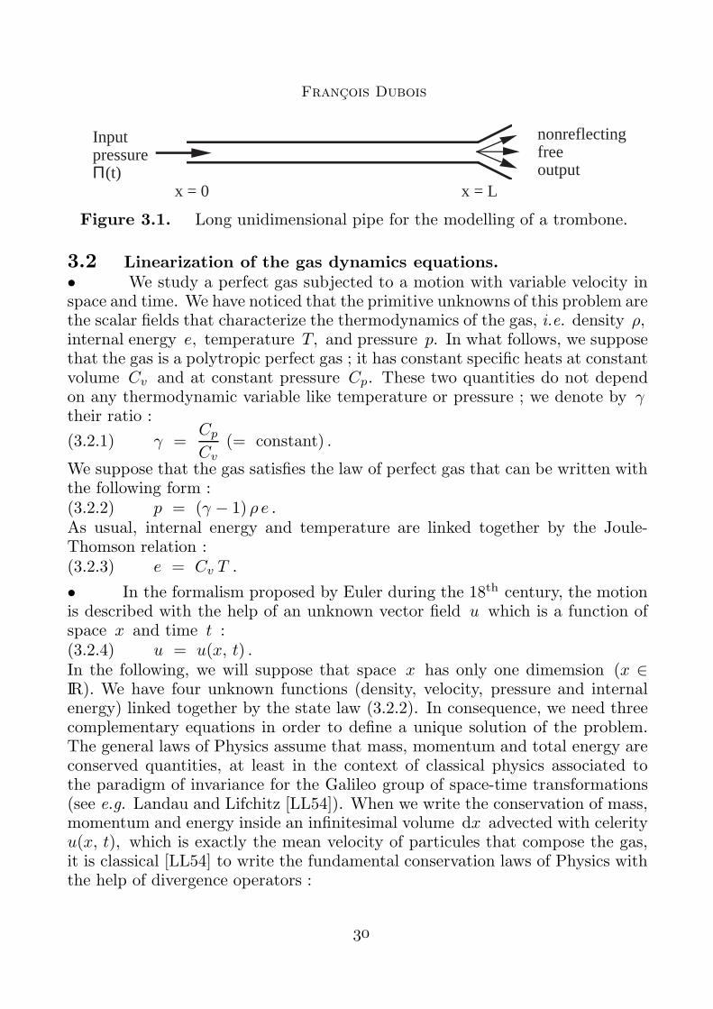
3) Gas dynamics with the Roe method.3.1 Nonlinear acoustics in one space dimension.• We propose here to describe quickly a physical problem that comesfrom the theoretical modelling of trombone, detailed for instance in the workof Hirschberg et al [HGMW96] or in our study [MD99] with R. Msallam. In afirst approximation, the duct of a trombone is a long cylinder with a constantsection and the acoustic waves propagate only in the longitudinal direction. Wecan use a one-dimensional description of the geometry (see Figure 3.1) and inwhat follows, the trombone is modelled by a real space variable x that rangesfrom x=0 at the input to x=L at the output.
• At the input x=0, a given non-stationary pressure wave t 7−→ Π(t) isemitted ; this wave is a perturbation of the ambiant pressure p0 of the air :(3.1.1) |Π(t)− p0 | << p0 , t > 0 .At the output x = L, the waves go outside without any reflection due to thepresence of a pavilion and the boundary condition is a “free output” and a non-reflecting boundary condition has to be used. At the initial time t=0, wecan consider that the air satisfies the usual conditions of pressure p(x, 0) ≡ p0 ,temperature T (x, 0) ≡ T0 and density ρ(x, 0) ≡ ρ0. We study in this section afinite volume method able to treat nonlinearities in the acoustic modelling andbased on the characteristic decompositions developed in the previous section.
Francois Dubois
Input pressureΠ(t)
nonreflectingfreeoutput
x = 0 x = L
Figure 3.1. Long unidimensional pipe for the modelling of a trombone.
3.2 Linearization of the gas dynamics equations.• We study a perfect gas subjected to a motion with variable velocity inspace and time. We have noticed that the primitive unknowns of this problem arethe scalar fields that characterize the thermodynamics of the gas, i.e. density ρ,internal energy e, temperature T, and pressure p. In what follows, we supposethat the gas is a polytropic perfect gas ; it has constant specific heats at constantvolume Cv and at constant pressure Cp. These two quantities do not dependon any thermodynamic variable like temperature or pressure ; we denote by γtheir ratio :
(3.2.1) γ =Cp
Cv(= constant) .
We suppose that the gas satisfies the law of perfect gas that can be written withthe following form :(3.2.2) p = (γ − 1) ρ e .As usual, internal energy and temperature are linked together by the Joule-Thomson relation :(3.2.3) e = Cv T .
• In the formalism proposed by Euler during the 18th century, the motionis described with the help of an unknown vector field u which is a function ofspace x and time t :(3.2.4) u = u(x, t) .In the following, we will suppose that space x has only one dimemsion (x ∈IR). We have four unknown functions (density, velocity, pressure and internalenergy) linked together by the state law (3.2.2). In consequence, we need threecomplementary equations in order to define a unique solution of the problem.The general laws of Physics assume that mass, momentum and total energy areconserved quantities, at least in the context of classical physics associated tothe paradigm of invariance for the Galileo group of space-time transformations(see e.g. Landau and Lifchitz [LL54]). When we write the conservation of mass,momentum and energy inside an infinitesimal volume dx advected with celerityu(x, t), which is exactly the mean velocity of particules that compose the gas,it is classical [LL54] to write the fundamental conservation laws of Physics withthe help of divergence operators :
An introduction to finite volumes for gas dynamics
(3.2.5)∂ρ
∂t+
∂
∂x
(ρu)
= 0
(3.2.6)∂
∂t
(ρu)
+∂
∂x
(ρu2 + p
)= 0
(3.2.7)∂
∂t
(12ρu2 + ρ e
)+
∂
∂x
( (12ρu2 +
p
γ − 1
)u + pu
)= 0 .
• We introduce the specific total energy E by unity of volume(3.2.8) E = 1
2u2 + e ,
the sound celerity c following the classical expression :
(3.2.9) c =
√γ p
ρ,
and total enthalpy H defined according to(3.2.10) H ≡ E + p
ρ = 12u
2 + 1γ−1 c
2 .
The vector W is therefore composed by the “conservative variables” or moreprecisely by the “conserved variables” :
(3.2.11) W =(ρ , ρ u , ρE
)t ≡(ρ , q , ǫ
)t.
The conservation laws (3.2.5)-(3.2.7) take the following general form of a systemof conservation laws :
(3.2.12)∂W
∂t+
∂
∂xF (W ) = 0
where the flux vector W 7−→ F (W ) satisfies the following algebraic expression :
(3.2.13) F (W ) =(ρu , ρ u2 + p , ρ uH
)tthat can be explicited as a true function of state vector W, on one hand withthe pressure law P (W ) computed with (3.2.2), (3.2.8) and (3.2.11) :
(3.2.14) P (W ) = (γ−1)
(ǫ− q2
2 ρ
)
and on the other hand with an explicit use of the conserved variables ρ, q andǫ. We obtain :
(3.2.15) F (W ) =(q ,
q2
ρ+ P (W ) ,
q ǫ
ρ+ P (W )
q
ρ
).
Proposition 3.1. Jacobian matrix of gas dynamics.• The Jacobian matrix dF (W ) of the flux function W 7−→ F (W ) for theEuler equations of the gas dynamics admits the following expression :
(3.2.16) dF (W ) =
0 1 0(γ−1)H − u2 − c2 (3− γ)u γ − 1(γ−2)uH − u c2 H − (γ−1)u2 γu
.
• The matrix dF (W ) is diagonalizable ; the eigenvalues λj(W ) satisfy therelations
Francois Dubois
(3.2.17) λ1(W ) ≡ u− c < λ2(W ) ≡ u < λ3(W ) ≡ u+ c .and the associated eigenvectors rj(W ) are proportional to the following ones :
(3.2.18) r1(W ) =
1u− cH − u c
, r2(W ) =
1u
12u
2
, r3(W ) =
1u+ cH + u c
.
• We first differentiate the pressure law W 7−→ P (W ) given in (3.2.14) :
(3.2.19)∂P
∂ρ=
γ−1
2u2 = (γ−1)H−c2 , ∂P
∂q= −(γ−1)u , ∂P
∂ǫ= (γ−1)
and the second row of the matrix (3.2.16) is a direct consequence of the relations∂
∂ρ
(q2ρ
)= −u2 and
∂
∂q
(q2ρ
)= 2u .
• The calculus of the third row of matrix in (3.2.16) demands first evalu-ation of the gradient of ρuE = u ǫ relatively to the state W. We get
(3.2.20)∂
∂ρ
(q ǫρ
)= −uE , ∂
∂q
(q ǫρ
)= E ,
∂
∂ǫ
(q ǫρ
)= u .
We have also ∂∂W (P u) = ∂P
∂W u + p ∂∂W
(qρ
)then we deduce from (3.2.19)
and the following expressions for the gradient of velocity ∂∂ρ
(qρ
)= −u
ρ and
∂∂q
(qρ
)= 1
ρ :
(3.2.21)
∂
∂ρ
(P qρ
)=
γ−1
2u3 − u p
ρ,
∂
∂q
(P qρ
)= −(γ−1)u2 +
p
ρ,
∂
∂ǫ
(P qρ
)= (γ−1)u .
We add the relations (3.2.20) and (3.2.21) ; then the third row of matrix (3.2.16)admits the following expression :
(γ−12 u3 − uH , H − (γ−1)u2 , γ u
)and
this result is exactly the third row of the right hand side of (3.2.16) when wetake into account the relation (3.2.10) between H, u2 and c2. The relations(3.2.17) and (3.2.18) are elementary to satisfy ; they express simply the threerelations :(3.2.22) dF (W ) • rj(W ) = λj(W ) rj(W ) , j = 1, 2, 3and Proposition 3.1 is established.
• We keep into memory the following expression of the Jacobian matrixdF (W ) :
(3.2.23) dF (W ) =
0 1 0γ−32 u2 (3− γ)u γ − 1
γ−12 u3 − uH H − (γ−1)u2 γu
that needs only the datum of velocity u and total enthalpy H of the state W.
An introduction to finite volumes for gas dynamics
3.3 Roe matrix.• We consider two states Wleft ≡ Wl and Wright ≡ Wr relatively to thegas dynamics, i.e. they both belong to space IR3 and have an expression ofthe form (3.2.11). By definition, a Roe matrix A(Wl, Wr) between these twostates is a 3 by 3 matrix that satisfy the three following properties :(3.3.1) A(Wl, Wr) is a diagonalizable matrix on the field IR of real numbers(3.3.2) A(W, W ) = dF (W )(3.3.3) F (Wr)− F (Wl) = A(Wl, Wr) • (Wr −Wl) .In his original article, P. Roe [Roe81] has proposed a very simple algebraic wayto construct a Roe matrix for the dynamics of polytropic gas. We propose it inthe following Proposition.
Proposition 3.2. Algebraic construction of a Roe matrix [Roe81].Let Wl and Wr be two states for gas dynamics, defined by their densities ρland ρr, their velocities ul and ur and their total enthalpies Hl and Hr. Weintroduce an intermediate state W ∗(Wl, Wr) by its density ρ∗, its velocityu∗ and its total enthalpy H∗ according to the following relations :(3.3.4) ρ∗ =
√ρl ρr
(3.3.5) u∗ =
√ρl ul +
√ρr ur√
ρl +√ρr
(3.3.6) H∗ =
√ρlHl +
√ρrHr√
ρl +√ρr
.
Then the matrix A(Wl, Wr) defined as the Jacobian matrix of the flux for theintermediate state W ∗(Wl, Wr), i.e.(3.3.7) A(Wl, Wr) = dF
(W ∗(Wl, Wr)
)
is a Roe matrix.
• Due to the expression (3.2.23) of the Jacobian matrix of gas dynamics,we remark that the formula (3.3.4) giving the density ρ∗ is not necessary for thedetermination of the matrix dF (W ∗(Wl, Wr)) and an entire family of statesW ∗(Wl, Wr) define a Roe matrix according to the relations (3.3.5), (3.3.6) and(3.3.7). Nevertheless, we keep this definition of density ρ∗ by convenience andsimplicity for future algebraic expressions. The proof of Proposition 3.2 needssome algebraic developments. We begin by the following technical lemma.
Proposition 3.3.Under the hypotheses of Proposition 3.2, we have the following relations :(3.3.8) (u∗)2 (ρr − ρl) − 2u∗ (ρr ur − ρl ul) + (ρr u
2r − ρl u
2l ) = 0
(3.3.9)
{−u∗H∗ (ρr − ρl) + H∗ (ρr ur − ρl ul) + u∗ (ρrHr − ρlHl) =
= ρr urHr − ρl ulHl .
Francois Dubois
• We first evaluate the left hand side of relation (3.3.8) :(u∗)2 (ρr − ρl) − 2u∗ (ρr ur − ρl ul) + (ρr u
2r − ρl u
2l ) =
= u∗(√ρr−
√ρl) (
√ρr ur+
√ρl ul)− 2u∗(ρr ur−ρl ul) + (ρr u
2r−ρl u2l )
= u∗(√ρl (
√ρl +
√ρr)ul −
√ρr (
√ρl +
√ρr)ur
)+ (ρr u
2r − ρl u
2l )
= (√ρl ul +
√ρr ur) (
√ρl ul −
√ρr ur) + (ρr u
2r − ρl u
2l )
= 0 and the relation (3.3.8) is established.
• We work on the left hand side of (3.3.9) as follows :−u∗H∗ (ρr − ρl) + H∗ (ρr ur − ρl ul) + u∗ (ρrHr − ρlHl) == −u∗(√ρr −
√ρl) (
√ρlHl+
√ρrHr) + H∗ (ρr ur −ρl ul) + u∗ (ρrHr −ρlHl)
=√ρl ρr u
∗ (Hr −Hl) + H∗ (ρr ur − ρl ul)
=
√ρl√ρr (
√ρl ul +
√ρr ur) (−Hl +Hr) + (−ρl ul + ρr ur) (
√ρlHl +
√ρrHr)√
ρl +√ρr
=1√
ρl +√ρr
[−ρl (
√ρl +
√ρr)ulHl + ρr (
√ρl +
√ρr)urHr
]
= ρr urHr − ρl ulHl
and the proposition 3.3 is established.
• The proof of Proposition 3.2 consists in satisfying the three hypothe-ses that define a Roe matrix. First, due to the fact that the relation (3.3.7)defines the matrix A(Wl, Wr) as a Jacobian of some state, this matrix is diag-onalizable with real elements due to the result of Proposition 3.1 and the firstproperty (3.3.1) is satisfied. The second property (3.3.2) is a simple consequenceof the fact that if Wl = Wr = W, then we have from the relations (3.3.4) to(3.3.6) : W ∗(Wl, Wr) = W and the property results from (3.3.7).
• The third property (3.3.3) needs more work. We remark that the firstrow of this matricial relation is clear. For the second row, we have :Second row of matrix A(Wl, Wr) • (Wr −Wl) =
=γ−3
2(u∗)2 (ρr − ρl) + (3−γ)u∗ (ρr ur − ρl ul) + (γ−1) (ρr Er − ρlEl)
=γ−3
2
[(u∗)2 (ρr −ρl) − 2u∗ (ρr ur −ρl ul)
]+γ−1
2(ρr u
2r −ρl u2l ) + (pr − pl)
= (ρr u2r − ρl u
2l ) + (pr − pl) due to (3.3.8)
= second row of the flux difference F (Wr)− F (Wl) .
• We have also, in consequence of (3.2.23),Third row of matrix A(Wl, Wr) • (Wr −Wl) =
= u∗(γ−1
2(u∗)2 −H∗
)(ρr − ρl) + (H∗ − (γ−1) (u∗)2) (ρr ur − ρl ul)+
+ γ u∗ (ρr Er − ρlEl)
=γ−1
2u∗[(u∗)2 (ρr − ρl) − 2u∗ (ρr ur − ρl ul)
]+
An introduction to finite volumes for gas dynamics
+[−H∗ u∗ (ρr − ρl) + H∗ (ρr ur − ρl ul)
]+ γ u∗ (ρr Er − ρlEl)
=γ−1
2u∗[(u∗)2 (ρr − ρl) − 2u∗ (ρr ur − ρl ul)
]− u∗ (ρrHr − ρlHl)+
+ (ρr urHr−ρl ulHl) + γ u∗ (ρr Er−ρl El) due to (3.3.9)
=γ−1
2u∗[(u∗)2 (ρr − ρl) − 2u∗ (ρr ur − ρl ul) + ρr u
2r − ρl u
2l
]+
+u∗ (−γ ρr er + γ ρl el + γ ρr er − γ ρl el) + ρr urHr − ρl ulHl
= ρr urHr−ρl ulHl due to (3.3.8)= third row of the flux difference F (Wr)− F (Wl)in the view of relation (3.2.13). The proposition 3.2 is established.
3.4 Roe flux.• The principal interest of the Roe matrix is to be able to use all what hasbeen developed for linear hyperbolic systems in Section 2. In particular, thefollowing linear hyperbolic system defined with a given Roe matrix A(Wl, Wr)
(3.4.1)∂W
∂t+ A(Wl, Wr) •
∂W
∂x= 0
can be treated with the upwind scheme defined at proposition 2.7. We obtainby doing this the following
Proposition 3.4. Three formulae for a flux.• Let Wl and Wr be two fluid states and W ∗ the intermediate statedefined by the relations (3.3.4) to (3.3.6). The sound celerity c∗ of state W ∗
is defined with the help of relation (3.2.10), i.e.
(3.4.2) c∗ =
√(γ−1)
(H∗ − (u∗)2
2
),
and the eigenvalues λ∗j of the Roe matrix A(Wl, Wr) ≡ dF (W ∗(Wl, Wr))are given by a relation analogous to (3.2.17).(3.4.3) λ∗1 ≡ u∗ − c∗ < λ∗2 ≡ u∗ < λ∗3 ≡ u∗ + c∗ .The associated eigenvectors r∗j ≡ rj(W
∗) are proportional to the followingones :
(3.4.4) r∗1 =
1u∗ − c∗
H∗ − u∗ c∗
, r∗2 =
1u∗
12 (u
∗)2
, r∗3 =
1u∗ + c∗
H∗ + u∗ c∗
.
• We introduce the decomposition of vector Wr −Wl in the basis r∗j :
(3.4.5) Wr −Wl =∑j=3
j=1 αj r∗j .
The three following relations define a unique numerical flux Φ(Wl, Wr) namedthe Roe flux between the two states Wl and Wr :(3.4.6) Φ(Wl, Wr) = F (Wl) +
∑j=3j=1 (λ
∗j )
− αj r∗j
(3.4.7) Φ(Wl, Wr) = F (Wr) − ∑j=3j=1 (λ
∗j )
+ αj r∗j
Francois Dubois
(3.4.8) Φ(Wl, Wr) = 12
(F (Wl) + F (Wr)
)− 1
2 |A(Wl, Wr) | • (Wr −Wl
).
• The first non-obvious point is to verify that the relation (3.4.2) definesa real number c∗. We have
H∗ − (u∗)2
2=
√ρlHl +
√ρrHr√
ρl +√ρr
− 1
2
( √ρl ul +
√ρr ur√
ρl +√ρr
)2=
=1
(√ρl +
√ρr)2
[(√ρl+
√ρr)(√
ρl(12u2l +
1
γ−1c2l)+
√ρr(12u2r+
1
γ−1c2r) )
− 1
2
(ρl u
2l + 2 ρ∗ ul ur + ρr u
2r
) ]
=1
(√ρl +
√ρr)2
[ 12
(ρ∗ u2l − 2 ρ∗ ul ur + ρ∗ u2r
)+
ρl + ρ∗
γ−1c2l +
ρ∗ + ρrγ−1
c2r
]
=1
(√ρl +
√ρr)2
[ 12ρ∗ (ur − ul)
2 +ρl + ρ∗
γ−1c2l +
ρ∗ + ρrγ−1
c2r
]> 0
and
(3.4.9) c∗ =
√γ−12 ρ∗ (ur − ul)2 + (ρl + ρ∗) c2l + (ρ∗ + ρr) c2r
√ρl +
√ρr
.
• We make the difference between the right hand sides of (3.4.6) and (3.4.7).We get :
F (Wr)− F (Wl) − ∑j=3j=1
((λ∗j )
+ + (λ∗j )−)αj r
∗j =
= A(Wl, Wr) • (Wr −Wl) − ∑j=3j=1 λ
∗j αj r
∗j due to (3.3.3) and (2.7.11)
= A(Wl, Wr) •(∑j=3
j=1 αj r∗j
)− ∑j=3
j=1 λ∗j αj r
∗j due to (3.4.5)
= 0 because A(Wl, Wr) • r∗j = λ∗j r
∗j for each integer j.
The proof of relation (3.4.8) is obtained by taking the half sum of (3.4.6) and(3.4.7). It is analogous to the one done for Proposition 2.7. The proof of Propo-sition 3.4 is completed.
• We make explicit the parameters αj introduced in relation (3.4.5)in order to be complete for the implementation of the above formulae on acomputer.
Proposition 3.5. New acoustic impedance.With the notations introduced at Proposition 3.4, and denoting by pl and prthe respective pressures of states Wl and Wr, we have the following relations forthe scalar components αj of the state difference Wr −Wl in relation (3.4.5) :
(3.4.10) α1 =1
2 (c∗)2[(pr − ρ∗ c∗ ur) − (pl − ρ∗ c∗ ul)
]
(3.4.11) α2 = − 1
(c∗)2[(pr − (c∗)2 ρr) − (pl − (c∗)2 ρl)
]
An introduction to finite volumes for gas dynamics
(3.4.12) α3 =1
2 (c∗)2[(pr + ρ∗ c∗ ur) − (pl + ρ∗ c∗ ul)
]
with acoustic impedance ρ∗ c∗ that is nomore the one ρ0 c0 of a referencestate as in traditional acoustics but an impedance associated with the Roe in-termediate state W ∗(Wl, Wr) of relations (3.3.4) to (3.3.6).
• We have just to explicit the three components of the relation (3.4.5). Itcomes :
ρr − ρl
ρr ur − ρl ulρr Er − ρlEl
=
α1 + α2 + α3
α1 (u∗ − c∗) + α2 u
∗ + α3 (u∗ + c∗)
α1 (H∗ − u∗ c∗) + α2
(u∗)2
2 + α3 (H∗ + u∗ c∗)
(3.4.13) α1 + α2 + α3 = ρr − ρl ,and we deduce after multiplying the equation (3.4.13) by −u∗ and adding tothe second equation of the above matrix equality :c∗ (α3 − α1) = ρr ur − ρl ul − u∗ (ρr − ρl)
= ρr ur − ρl ul − (√ρr −
√ρl) (
√ρl ul +
√ρr ur) ,
then(3.4.14) c∗ (−α1 + α3) = ρ∗ (ur − ul) .
• We deduce from the third equation of relation (3.4.5) :(c∗)2
γ−1(α1 + α3) = ρr Er − ρlEl −
1
2(u∗)2 (ρr − ρl) − u∗ c∗ (α3 − α1)
=1
γ−1(pr −pl) +
1
2(ρr u
2r −ρl u2l ) +
1
2(u∗)2 (ρr −ρl) − u∗ (ρr ur −ρl ul)
=1
γ−1(pr − pl) due to (3.3.8). Then we have :
(3.4.15) (c∗)2 (α1 + α3) = pr − pl .
• The solution of the 2 by 2 linear system with unknowns α1 and α3
defined by the relations (3.4.14) and (3.4.15) directly gives the relations (3.4.10)and (3.4.12). The expression (3.4.11) of variable α2 is a direct consequence ofthe relations (3.4.10), (3.4.12) and (3.4.13) and Proposition 3.5 is proven.
Proposition 3.6. An algorithm for the Roe flux.Let Wl and Wr be two compressible fluid states. The computation of theRoe flux Φ(Wl, Wr) of relations (3.4.6)-(3.4.8) between these two states issummarized by the following points :• Evaluation of density ρ∗, velocity u∗ and total enthalpy H∗ of theintermediate state W ∗ with the relations (3.3.4) to (3.3.6),• Determination of the sound celerity c∗ of the intermediate state W ∗ fromthe previous data with the relation (3.4.2),• Eigenvectors r∗j of the Roe matrix with the relations (3.4.4),
Francois Dubois
• Computation of the characteristic variables αj in (3.4.5) for the differenceWr −Wl with the relations (3.4.10) to (3.4.12),• Final computation of the Roe flux Φ(Wl, Wr) with the minimum of work :(3.4.16) Φ(Wl, Wr) = F (Wl) if u∗ − c∗ ≥ 0(3.4.17) Φ(Wl, Wr) = F (Wl) + (u∗− c∗) α1 r
∗1 if u∗− c∗ ≤ 0 < u∗
(3.4.18) Φ(Wl, Wr) = F (Wr) − (u∗+c∗) α3 r∗3 if u∗ ≤ 0 < u∗+c∗
(3.4.19) Φ(Wl, Wr) = F (Wr) if u∗ + c∗ ≤ 0 .
• The proof of the relations (3.4.16)-(3.4.19) is obtained by starting fromthe expression of the Roe flux given in (3.4.6). We know that λ1 = u∗ − c∗,λ2 = u∗, λ3 = u∗ + c∗. If u∗ − c∗ ≥ 0, then u∗ ≥ 0 and u∗ + c∗ ≥ 0, so therelation (3.4.6) reduces to (3.4.16) because, due to (2.7.10), µ− = 0 if µ is apositive real number. If u∗−c∗ ≤ 0 < u∗ < u∗+c∗, the term containing (λ∗1)
−
is the only one that contributes in relation (3.4.6) and the relation (3.4.17) is adirect consequence of this remark. If u∗ − c∗ < u∗ ≤ 0 < u∗ + c∗, the termthat contains (λ∗3)
+ is the only nonzero element among the three inside therelation (3.4.7) and we deduce the relation (3.4.18) from this property. Whenu∗ − c∗ < u∗ < u∗ + c∗ ≤ 0, the term F (Wr) is the only to subsist inside therelation (3.4.7) and the relation (3.4.19) is established. We remark also that thealgebraic expression (3.4.11) for α2 is not necessary for the implementation ofthe algorithm.
3.5 Entropy correction.• The Roe flux replaces the nonlinear waves of the gas dynamics, i.e.the rarefactions and the shock waves by linear waves that are the contactdiscontinuities. If sufficiently weak shock waves occur for a given discontinuitybetween two states Wleft and Wright, the Roe flux presented above is a goodapproximation, but if a rarefaction containing a sonic point is present amongthe nonlinear waves that solves the discontinuity problem between Wleft andWright, it has been early remarked that for this very particular situation, theRoe flux does not satisfy the entropy condition (see e.g. Godlewski and Raviart[GR96]).
• A popular response has been proposed by Harten [Ha83] with a tuningparameter that plays in fact the role of an artificial viscosity and P. Roe himself[Roe85] has proposed a nonparameterized entropy correction for his flux. WithG. Mehlman, we have treated the same subject by the introduction of hyperbolicnonlinear models with nonconvex flux functions and have proved a discrete en-tropy inequality if sufficiently weak nonlinear waves are present in the problem[DM96]. We detail here the modification of the algorithm that we have proposedand tested numerically for various gas dynamics problems.
An introduction to finite volumes for gas dynamics
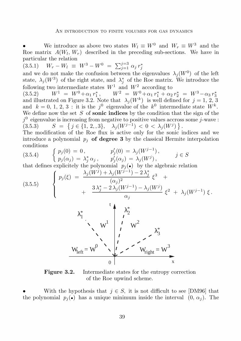
• We introduce as above two states Wl ≡ W 0 and Wr ≡ W 3 and theRoe matrix A(Wl, Wr) described in the preceding sub-sections. We have inparticular the relation
(3.5.1) Wr −Wl ≡ W 3 −W 0 =∑j=3
j=1 αj r∗j
and we do not make the confusion between the eigenvalues λj(W0) of the left
state, λj(W3) of the right state, and λ∗j of the Roe matrix. We introduce the
following two intermediate states W 1 and W 2 according to(3.5.2) W 1 = W 0+α1 r
∗1 , W 2 = W 0+α1 r
∗1 + α2 r
∗2 = W 3−α3 r
∗3
and illustrated on Figure 3.2. Note that λj(Wk) is well defined for j = 1, 2, 3
and k = 0, 1, 2, 3 : it is the j0 eigenvalue of the k0 intermediate state W k.We define now the set S of sonic indices by the condition that the sign of thej0 eigenvalue is increasing from negative to positive values accross some j-wave :(3.5.3) S =
{j ∈ {1, 2, , 3}, λj(W
j−1) < 0 < λj(Wj)}.
The modification of the Roe flux is active only for the sonic indices and weintroduce a polynomial pj of degree 3 by the classical Hermite interpolationconditions
(3.5.4)
{pj(0) = 0 , p′j(0) = λj(W
j−1) ,
pj(αj) = λ∗j αj , p′j(αj) = λj(Wj) ,
j ∈ S
that defines explicitely the polynomial pj(•) by the algebraic relation
(3.5.5)
pj(ξ) =λj(W
j) + λj(Wj−1)− 2λ∗j
(αj)2ξ3 +
+3λ∗j − 2λj(W
j−1)− λj(Wj)
αjξ2 + λj(W
j−1) ξ .
t
x
W = Wright3
W = W0
left
λ1* λ2
*
λ3*
W2
W1
0
Figure 3.2. Intermediate states for the entropy correctionof the Roe upwind scheme.
• With the hypothesis that j ∈ S, it is not difficult to see [DM96] thatthe polynomial pj(•) has a unique minimum inside the interval (0, αj). The
Francois Dubois
argument ξ∗j of this point of minimum is given according to :
(3.5.6) ξ∗j =−λj(W j−1) αj( (
3λ∗j − 2λj(Wj−1)− λj(W
j))+
+
√(3λ∗j − λj(W j)− λj(W j−1)
)2 − λj(W j−1)λj(W j)
) .
Since pj(ξ∗j) is the unique minimum of the polynomial pj(•) on the inter-
val (0, αj), we havepj(ξ
∗
j)
αj≤ 0 and
pj(ξ∗
j)
αj≤ λ∗j . Then the modified flux
Φmodif(Wl, Wr) is defined from the Roe flux Φ(Wl, Wr) by the relation
(3.5.7) Φmodif(Wl, Wr) = Φ(Wl, Wr)+∑
j∈S
max
(pj(ξ∗j)
αj,pj(ξ∗j)
αj−λ∗j
)αj r
∗j
that makes the added numerical viscosity explicit.
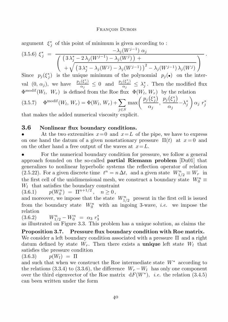
3.6 Nonlinear flux boundary conditions.• At the two extremities x=0 and x=L of the pipe, we have to expresson one hand the datum of a given nonstationary pressure Π(t) at x=0 andon the other hand a free output of the waves at x=L.
• For the numerical boundary condition for pressure, we follow a generalapproach founded on the so-called partial Riemann problem [Du01] thatgeneralizes to nonlinear hyperbolic systems the reflection operator of relation(2.5.22). For a given discrete time tn = n∆t, and a given state Wn
1/2 ≡Wr in
the first cell of the unidimensional mesh, we construct a boundary state Wn0 ≡
Wl that satisfies the boundary constraint(3.6.1) p(Wn
0 ) = Πn+1/2 , n ≥ 0 ,and moreover, we impose that the state Wn
1/2 present in the first cell is issued
from the boundary state Wn0 with an ingoing 3-wave, i.e. we impose the
relation(3.6.2) Wn
1/2 −Wn0 = α3 r
∗3
as illustrated on Figure 3.3. This problem has a unique solution, as claims the
Proposition 3.7. Pressure flux boundary condition with Roe matrix.We consider a left boundary condition associated with a pressure Π and a rightdatum defined by state Wr. Then there exists a unique left state Wl thatsatisfies the pressure condition(3.6.3) p(Wl) = Πand such that when we construct the Roe intermediate state W ∗ according tothe relations (3.3.4) to (3.3.6), the difference Wr −Wl has only one componentover the third eigenvector of the Roe matrix dF (W ∗), i.e. the relation (3.4.5)can been written under the form
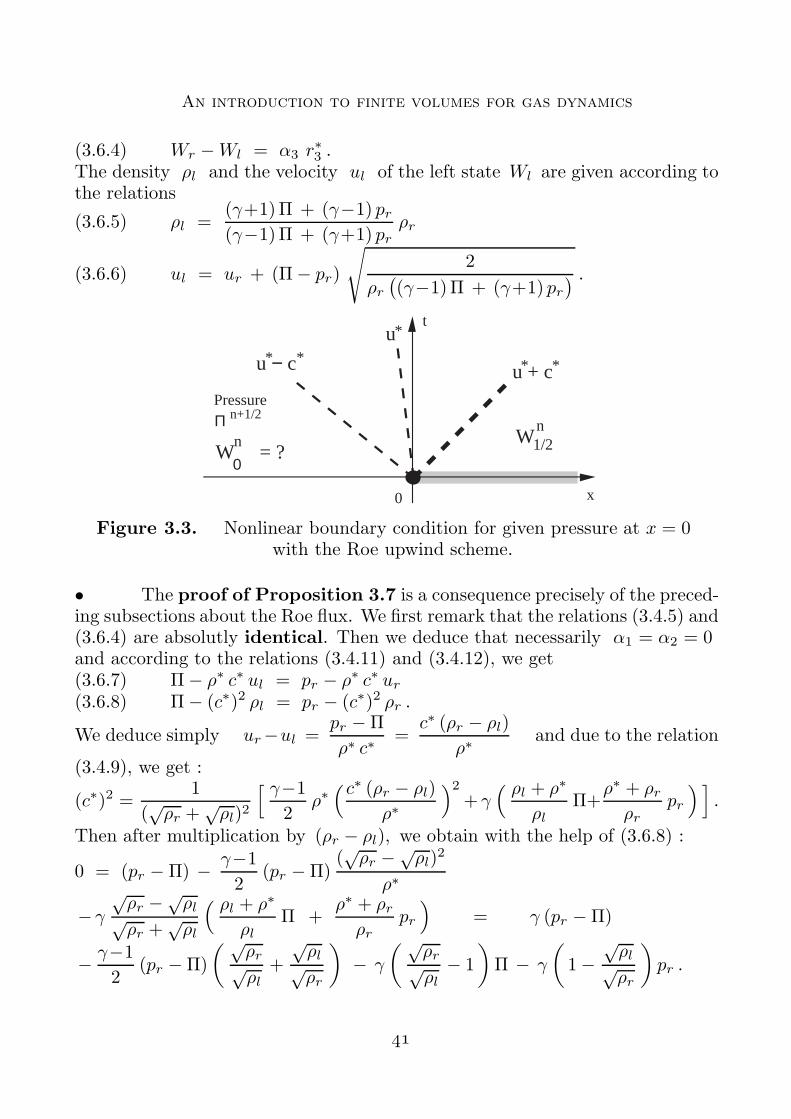
An introduction to finite volumes for gas dynamics
(3.6.4) Wr −Wl = α3 r∗3 .
The density ρl and the velocity ul of the left state Wl are given according tothe relations
(3.6.5) ρl =(γ+1)Π + (γ−1) pr(γ−1)Π + (γ+1) pr
ρr
(3.6.6) ul = ur + (Π− pr)
√2
ρr((γ−1)Π + (γ+1) pr
) .
t
x
W1/2n
u*
u + c* *
0
u − c* *
W = ?0n
Pressure n+1/2Π
Figure 3.3. Nonlinear boundary condition for given pressure at x = 0with the Roe upwind scheme.
• The proof of Proposition 3.7 is a consequence precisely of the preced-ing subsections about the Roe flux. We first remark that the relations (3.4.5) and(3.6.4) are absolutly identical. Then we deduce that necessarily α1 = α2 = 0and according to the relations (3.4.11) and (3.4.12), we get(3.6.7) Π− ρ∗ c∗ ul = pr − ρ∗ c∗ ur(3.6.8) Π− (c∗)2 ρl = pr − (c∗)2 ρr .
We deduce simply ur−ul =pr −Π
ρ∗ c∗=
c∗ (ρr − ρl)
ρ∗and due to the relation
(3.4.9), we get :
(c∗)2 =1
(√ρr +
√ρl)2
[ γ−1
2ρ∗(c∗ (ρr − ρl)
ρ∗
)2+ γ
( ρl + ρ∗
ρlΠ+
ρ∗ + ρrρr
pr
) ].
Then after multiplication by (ρr − ρl), we obtain with the help of (3.6.8) :
0 = (pr − Π) − γ−1
2(pr −Π)
(√ρr −√
ρl)2
ρ∗
− γ√ρr −√
ρl√ρr +
√ρl
( ρl + ρ∗
ρlΠ +
ρ∗ + ρrρr
pr
)= γ (pr −Π)
− γ−1
2(pr −Π)
( √ρr√ρl
+
√ρl√ρr
)− γ
( √ρr√ρl
− 1
)Π − γ
(1−
√ρl√ρr
)pr .
Francois Dubois
We multiply the previous equality by√
ρl
ρrand we get :
−γ−1
2(pr − Π) ( 1 +
ρlρr
) − γΠ + γρlρrpr = 0 ,
id est[−γ−1
2(pr −Π) + γ pr
] ρlρr
= γΠ +γ−1
2(pr − Π)
and the relation (3.6.5) is established.
• We deduce from the previous relation :
ρ∗ =
√(γ+1)Π + (γ−1) pr(γ−1)Π + (γ+1) pr
ρr , ρr − ρl =2 (pr − Π)
(γ−1)Π + (γ+1) prρr
and due to the relation (3.6.8) :
(c∗)2 =(γ−1)Π + (γ+1) pr
2 ρr, ρ∗ c∗ =
√(γ−1)Π + (γ+1) pr
2
√ρr
and the relation (3.6.6) is an easy consequence of the last equality joined with(3.6.7). The proposition 3.7 is established.
• The determination of a nonlinear nonreflecting boundary conditionat x=L is still an open mathematical problem. We recommand for deriving aflux boundary condition for such a situation to impose that no wave are presentat the interaction for the last interface j=J. We just write
(3.6.9) fn+1/2J = F (Wn
J−1/2) , n ≥ 0which is equivalent of introducing a right boundary state Wn
J according to thesimple relation Wn
J = WnJ−1/2 and then making these two states interacting
with the Roe flux : fn+1/2J = Φ(Wn
J−1/2, WnJ ). This last definition is equivalent
to the one proposed in (3.6.9) due to the property (3.3.2) of the Roe matrix.
4) Second order and two space dimensions.4.1 Towards second order accuracy.• The finite volume method described in the previous sections is a naturalmethod for the discretization of systems of m conservation laws. It conductsto an explicit scheme in time : the evaluation of the field Wn+1 at time step(n+1)∆t needs only the knowledge of the field Wn
j+1/2 for j = 0, · · · , J−1
at the preceding time step n∆t. This evaluation needs a certain number ofauxiliary computations without the resolution of any linear system involving thenew field. The method is parameterized by the choice of a numerical flux and agreat flexibility can be adopted at this level. We have proposed two fluxes fornonlinear problems related to nonlinear acoustics and gas dynamics, the Roe flux
An introduction to finite volumes for gas dynamics
Φ(•, •) of relations (3.4.6)-(3.4.8) that conduct to a discrete scheme accordingto the relation(4.1.1) f
n+1/2j = Φ(Wn
j−1/2, Wnj+1/2) ,
and the modified Roe flux Φmodif(•, •) of relation (3.6.7) that enforces theentropy condition. This explicit version of the finite volume method is submittedto a stability condition that can be written as a first approximation for linearcases as :
(4.1.2) c0∆t
∆x≤ 1 .
• Nevertheless, the above finite volume method is only first order accu-rate. If we insert an exact solution W (x, t) of the conservation law
(4.1.3)∂W
∂t+
∂
∂xF (W ) = 0
inside the formal expression of the flux (4.1.1), it is easy to see that the finite
difference 1∆x (f
n+1/2j+1 − f
n+1/2j ) is first order accurate :
(4.1.4)1
∆x
(fn+1/2j+1 − f
n+1/2j
)=
(∂F (W )
∂x
)n+1/2
j+1/2
+ O(∆t+∆x
).
In a similar way, the use of an explicit scheme in time conducts to
(4.1.5)1
∆t(Wn+1
j+1/2 −Wnj+1/2) +
1
∆x
(fn+1/2j+1 − f
n+1/2j
)= 0
and maintains this first order accuracy for the finite volume scheme.
• We develop in this section the fact that it is possible to improve themethod, i.e. to define a method with a relation of the type (4.1.5), and thatconduct to a troncation error of second order :
(4.1.6)
1
∆t(Wn+1
j+1/2 −Wnj+1/2) +
1
∆x
(fn+1/2j+1 − f
n+1/2j
)=
=
(∂W
∂t+
∂
∂xF (W )
)n+1/2
j+1/2
+ O(∆t2 +∆x2
).
The price to pay is to develop flux formulae much more complicated than thesimple relation (4.1.1). When the second order precision (4.1.6) is achieved witha stable scheme, the precision is sufficient to develop predictive computations inacoustics and aerodynamics, whereas that is not the case with the initial scheme(4.1.1) (4.1.5).
4.2 The method of lines.• The simplest way to extend the first order finite volume scheme is first todevelop a new vision of the method with emphasis more on abstraction. We havepresented a method founded on the integration of the conservation law (4.1.3)
Francois Dubois
inside the space-time domain Vn+1/2j+1/2 = ]xj , xj+1[× ]tn, tn+1[ as suggested in
(2.1.6). With the method of lines, we just integrate the conservation (4.1.3)in space in each control volume Kj+1/2 = ]xj , xj+1[. It is straightforward tointroduce the mean value Wj+1/2(t) in this finite element :
(4.2.1) Wj+1/2(t) =1
| Kj+1/2 |
∫ xj+1
xjW (x, t) dx ;
then we integrate the conservation law (4.1.3) in space in the cell Kj+1/2 and
taking into account the relation ddtWj+1/2(t) = 1
∆x
∫ xj+1xj
∂W∂t (x, t) dx, we get
simply
(4.2.2)d
dtWj+1/2(t) +
1
∆x
[fj+1(t) − fj(t)
]= 0
with(4.2.3) fj(t) = F
(W (xj , t)
).
• As usual with the finite volume method, a numerical scheme can beobtained from the relations (4.2.2) (4.2.3) by replacing the relation (4.2.3) bysome explicit function over the set of all discrete variables introduced for therelation (4.2.1). To fix the ideas, we introduce a dynamic state vector Z(t)composed by all the dynamic variables on the finite mesh :(4.2.4) Z(t) =
(W1/2(t), · · · , Wj+1/2(t), · · · , WJ−1/2(t)
)∈ (IRm)J .
The discretization in space is achieved if we are able to determine the numericalflux fj(t) with the help of both the dynamic state vector Z(•) and the bound-ary conditions, that is the input pressure Π(t) in the example considered inthe last section. As in relation (2.1.12), we introduce a local numerical fluxfunction Ψj(•, •) relative to the vertex xj :(4.2.5) fj(t) = Ψj
(Π(t), Z(t)
).
We replace the relation (4.2.3) by the numerical approximation (4.2.5) insidethe equation (4.2.2) of dynamic evolution of the state variable Wj+1/2(•). Weobtain the following ordinary differential equation
(4.2.6)d
dtWj+1/2(t) +
1
∆x
[Ψj+1
(Π(t), Z(t)
)− Ψj
(Π(t), Z(t)
) ]= 0 .
• The method of lines is a semi-discrete version of the finite volumemethod. It is obtained by integration in space of the conservation law withoutintegration in time. The result is not a numerical scheme but just an ordinarydifferential equation for the dynamic state vector Z(•) described component bycomponent with the equation (4.2.6). The method is parameterized by the localnumerical flux functions Ψj
(•, •) and take the general form of a dynamical
system parameterized by the pressure function t 7−→ Π(t) :
(4.2.7)d
dtZ(t) = G(Z, t) .
An introduction to finite volumes for gas dynamics
The discrete dynamic function (IRm)J × [0, +∞[ ∋ (Z, t) 7→ G(Z, t) ∈(IRm)J is a vector valued expression with J components :(4.2.8) G(Z, t) =
(G1/2(Z, t), · · · , Gj+1/2(Z, t), · · · , GJ−1/2(Z, t)
)∈ (IRm)J
and it is defined from the (J+1) local numerical fluxes (Ψj)j=0, ···, J with thevery simple algebra relative to the finite volume method :
(4.2.9) Gj+1/2(Z, t) = − 1
∆x
(Ψj+1(Π(t), Z)−Ψj(Π(t), Z)
), 0 ≤ j ≤ J−1 .
Proposition 4.1. Explicit Euler scheme.With the choice of the first order scheme in space, that is(4.2.10) Ψj
(Πn, Zn
)= Φ(Wn
j−1/2, Wnj+1/2) if j = 1, · · · , J−1,
and the first order explicit forward Euler scheme for the ordinary differentialequation (4.2.7), id est
(4.2.11)1
∆t(Zn+1 − Zn) = G(Zn, tn) ,
we recover the previous first order finite volume scheme
(4.2.12)
1
∆t
(Wn+1
j+1/2 −Wnj+1/2
)+
1
∆x
(Φ(Wn
j+1/2, Wnj+3/2
)
− Φ(Wn
j−1/2, Wnj+1/2
))= 0 for j = 1, · · · , J−2.
• We write the relation (4.2.10) for the particular control volume Kj+1/2
and we get : Wn+1j+1/2 = Wn
j+1/2 + ∆t G(zn, tn) due to (4.2.11), then
Wn+1j+1/2 = Wn
j+1/2 − 1
∆x
(Ψj+1(Π
n, Zn) − Ψj(Πn, Zn)
)due to (4.2.9)
= Wnj+1/2 − 1
∆x
(Φ(Wn
j+1/2, Wnj+3/2)−Φ(Wn
j−1/2, Wnj+1/2)
)c.f. (4.2.10)
and the relation (4.2.12) is established.
4.3 The method of Van Leer.• We turn now to the construction of a second order accurate version of thefinite volume method as proposed initially with the “Multidimensional Upwind-centered Scheme for Conservation Laws” of B. Van Leer [VL79]. The fundamen-tal idea of this scheme is the reconstruction of a function IR ∋ x 7−→W (x) ∈ IRfrom his mean values Wj+1/2 in each cell Kj+1/2 . The reconstructed functionis regular inside each control volume Kj+1/2 and is discontinuous at the in-terfaces xl between two control volumes. The application to the finite volumemethod replaces the scheme (4.1.1) by the same Roe flux interaction Φ(•, •)considered for the two extrapolated data W−
j and W+j on each side of the
boundary :(4.3.1) fj = Φ(W−
j , W+j ) .
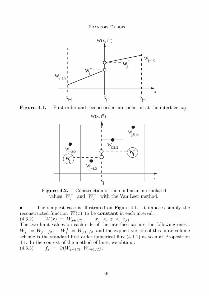
Francois Dubois
W(x, t )n
x
xj+1
xj
xj−1
Wj+1/2
Wj−1/2
Wj−
Wj+
Figure 4.1. First order and second order interpolation at the interface xj .
W(x, t )n
x
Wj−
AAAAAA
Wj−1/2
Wj−3/2
Wj+1/2
Wj+3/2
Wj+
AAAAAA
xj
Figure 4.2. Construction of the nonlinear interpolatedvalues W−
j and W+j with the Van Leer method.
• The simplest case is illustrated on Figure 4.1. It imposes simply thereconstructed function W (x) to be constant in each interval :(4.3.2) W (x) ≡ Wj+1/2 , xj < x < xj+1 .The two limit values on each side of the interface xj are the following ones :W−
j = Wj−1/2 , W+j = Wj+1/2 and the explicit version of this finite volume
scheme is the standard first order numerical flux (4.1.1) as seen at Proposition4.1. In the context of the method of lines, we obtain :(4.3.3) fj = Φ(Wj−1/2, Wj+1/2) .
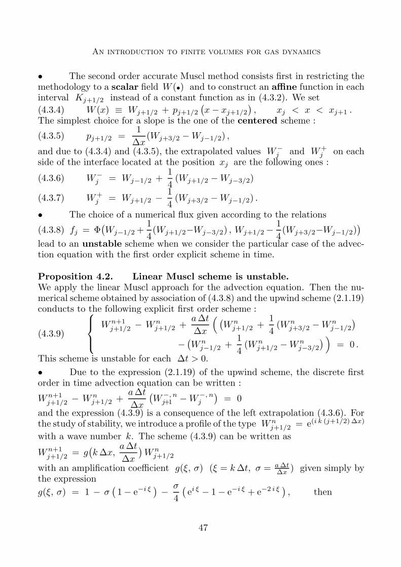
An introduction to finite volumes for gas dynamics
• The second order accurate Muscl method consists first in restricting themethodology to a scalar field W (•) and to construct an affine function in eachinterval Kj+1/2 instead of a constant function as in (4.3.2). We set
(4.3.4) W (x) ≡ Wj+1/2 + pj+1/2
(x− xj+1/2
), xj < x < xj+1 .
The simplest choice for a slope is the one of the centered scheme :
(4.3.5) pj+1/2 =1
∆x(Wj+3/2 −Wj−1/2) ,
and due to (4.3.4) and (4.3.5), the extrapolated values W−j and W+
j on eachside of the interface located at the position xj are the following ones :
(4.3.6) W−j = Wj−1/2 +
1
4(Wj+1/2 −Wj−3/2)
(4.3.7) W+j = Wj+1/2 − 1
4(Wj+3/2 −Wj−1/2) .
• The choice of a numerical flux given according to the relations
(4.3.8) fj = Φ(Wj−1/2 +
1
4(Wj+1/2−Wj−3/2) , Wj+1/2 −
1
4(Wj+3/2−Wj−1/2)
)
lead to an unstable scheme when we consider the particular case of the advec-tion equation with the first order explicit scheme in time.
Proposition 4.2. Linear Muscl scheme is unstable.We apply the linear Muscl approach for the advection equation. Then the nu-merical scheme obtained by association of (4.3.8) and the upwind scheme (2.1.19)conducts to the following explicit first order scheme :
(4.3.9)
Wn+1j+1/2 − Wn
j+1/2 +a∆t
∆x
( (Wn
j+1/2 +1
4(Wn
j+3/2 −Wnj−1/2
)
−(Wn
j−1/2 +1
4(Wn
j+1/2 −Wnj−3/2
) )= 0 .
This scheme is unstable for each ∆t > 0.
• Due to the expression (2.1.19) of the upwind scheme, the discrete firstorder in time advection equation can be written :
Wn+1j+1/2 − Wn
j+1/2 +a∆t
∆x
(W−, n
j+1 −W−, nj
)= 0
and the expression (4.3.9) is a consequence of the left extrapolation (4.3.6). Forthe study of stability, we introduce a profile of the type Wn
j+1/2 = e(i k (j+1/2)∆x)
with a wave number k. The scheme (4.3.9) can be written as
Wn+1j+1/2 = g
(k∆x,
a∆t
∆x
)Wn
j+1/2
with an amplification coefficient g(ξ, σ) (ξ = k∆t, σ = a∆t∆x ) given simply by
the expression
g(ξ, σ) = 1 − σ(1− e−i ξ
)− σ
4
(ei ξ − 1− e−i ξ + e−2 i ξ
), then
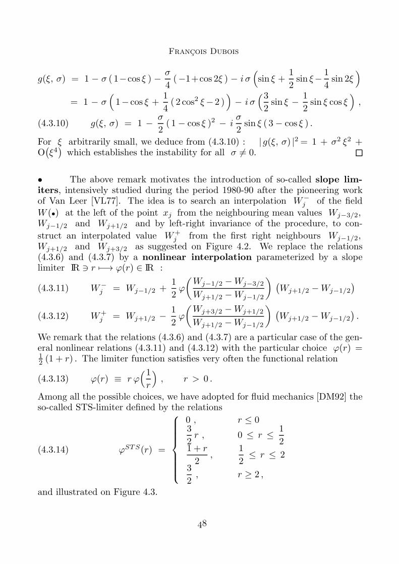
Francois Dubois
g(ξ, σ) = 1 − σ ( 1−cos ξ ) − σ
4(−1+cos 2ξ ) − i σ
(sin ξ +
1
2sin ξ− 1
4sin 2ξ
)
= 1 − σ(1− cos ξ +
1
4( 2 cos2 ξ−2 )
)− i σ
(32sin ξ − 1
2sin ξ cos ξ
),
(4.3.10) g(ξ, σ) = 1 − σ
2( 1− cos ξ )2 − i
σ
2sin ξ ( 3− cos ξ ) .
For ξ arbitrarily small, we deduce from (4.3.10) : |g(ξ, σ) |2 = 1 + σ2 ξ2 +O(ξ4)which establishes the instability for all σ 6= 0.
• The above remark motivates the introduction of so-called slope lim-iters, intensively studied during the period 1980-90 after the pioneering workof Van Leer [VL77]. The idea is to search an interpolation W−
j of the field
W (•) at the left of the point xj from the neighbouring mean values Wj−3/2,Wj−1/2 and Wj+1/2 and by left-right invariance of the procedure, to con-
struct an interpolated value W+j from the first right neighbours Wj−1/2,
Wj+1/2 and Wj+3/2 as suggested on Figure 4.2. We replace the relations(4.3.6) and (4.3.7) by a nonlinear interpolation parameterized by a slopelimiter IR ∋ r 7−→ ϕ(r) ∈ IR :
(4.3.11) W−j = Wj−1/2 +
1
2ϕ
(Wj−1/2 −Wj−3/2
Wj+1/2 −Wj−1/2
) (Wj+1/2 −Wj−1/2
)
(4.3.12) W+j = Wj+1/2 − 1
2ϕ
(Wj+3/2 −Wj+1/2
Wj+1/2 −Wj−1/2
) (Wj+1/2 −Wj−1/2
).
We remark that the relations (4.3.6) and (4.3.7) are a particular case of the gen-eral nonlinear relations (4.3.11) and (4.3.12) with the particular choice ϕ(r) =12 (1 + r) . The limiter function satisfies very often the functional relation
(4.3.13) ϕ(r) ≡ r ϕ(1r
), r > 0 .
Among all the possible choices, we have adopted for fluid mechanics [DM92] theso-called STS-limiter defined by the relations
(4.3.14) ϕSTS(r) =
0 , r ≤ 03
2r , 0 ≤ r ≤ 1
21 + r
2,
1
2≤ r ≤ 2
3
2, r ≥ 2 ,
and illustrated on Figure 4.3.
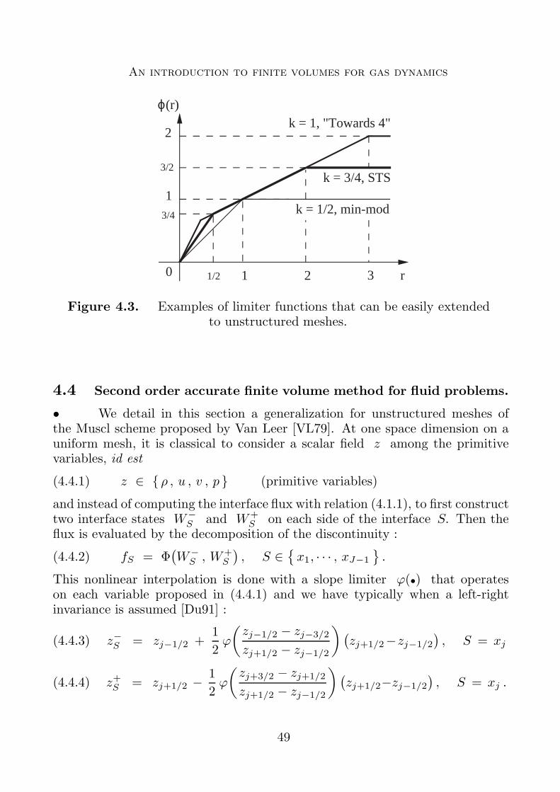
An introduction to finite volumes for gas dynamics
ϕ(r)
2
0
1
3 r21/2
k = 1, "Towards 4"
k = 3/4, STS
k = 1/2, min-mod3/4
3/2
1
Figure 4.3. Examples of limiter functions that can be easily extendedto unstructured meshes.
4.4 Second order accurate finite volume method for fluid problems.
• We detail in this section a generalization for unstructured meshes ofthe Muscl scheme proposed by Van Leer [VL79]. At one space dimension on auniform mesh, it is classical to consider a scalar field z among the primitivevariables, id est
(4.4.1) z ∈ { ρ , u , v , p } (primitive variables)
and instead of computing the interface flux with relation (4.1.1), to first constructtwo interface states W−
S and W+S on each side of the interface S. Then the
flux is evaluated by the decomposition of the discontinuity :
(4.4.2) fS = Φ(W−
S , W+S
), S ∈
{x1, · · · , xJ−1
}.
This nonlinear interpolation is done with a slope limiter ϕ(•) that operateson each variable proposed in (4.4.1) and we have typically when a left-rightinvariance is assumed [Du91] :
(4.4.3) z−S = zj−1/2 +1
2ϕ
(zj−1/2 − zj−3/2
zj+1/2 − zj−1/2
)(zj+1/2−zj−1/2
), S = xj
(4.4.4) z+S = zj+1/2 − 1
2ϕ
(zj+3/2 − zj+1/2
zj+1/2 − zj−1/2
)(zj+1/2−zj−1/2
), S = xj .
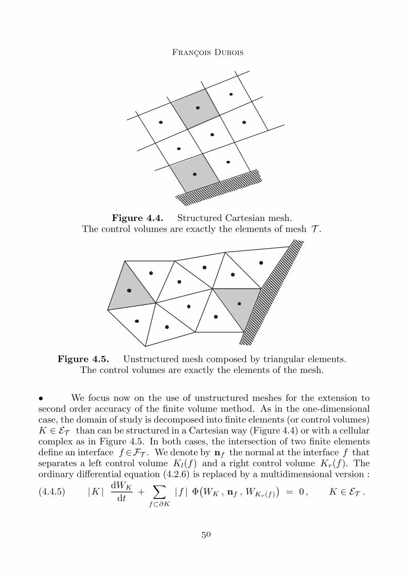
Francois Dubois
AAAAAAAAAAAAAAAAAAAAAAAAAAAAAAAA
Figure 4.4. Structured Cartesian mesh.The control volumes are exactly the elements of mesh T .
AAAAAAAAAAAAAAAAAAAAAAAAAAAAAAAAAAAAAAAAAAAAAAAA
Figure 4.5. Unstructured mesh composed by triangular elements.The control volumes are exactly the elements of the mesh.
• We focus now on the use of unstructured meshes for the extension tosecond order accuracy of the finite volume method. As in the one-dimensionalcase, the domain of study is decomposed into finite elements (or control volumes)K ∈ ET than can be structured in a Cartesian way (Figure 4.4) or with a cellularcomplex as in Figure 4.5. In both cases, the intersection of two finite elementsdefine an interface f ∈FT . We denote by nf the normal at the interface f thatseparates a left control volume Kl(f) and a right control volume Kr(f). Theordinary differential equation (4.2.6) is replaced by a multidimensional version :
(4.4.5) |K | dWK
dt+
∑
f⊂∂K
|f | Φ(WK , nf , WKr(f)
)= 0 , K ∈ ET .
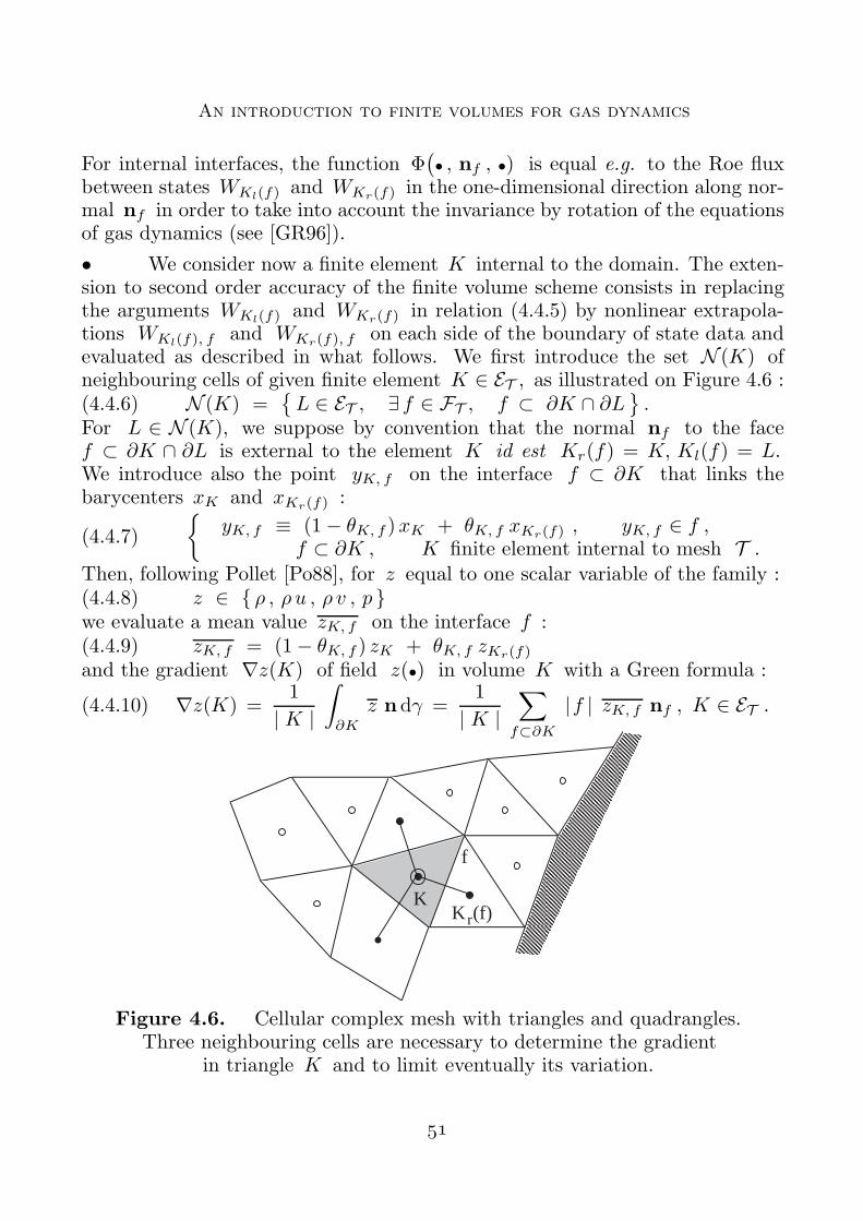
An introduction to finite volumes for gas dynamics
For internal interfaces, the function Φ(• , nf , •) is equal e.g. to the Roe flux
between states WKl(f) and WKr(f) in the one-dimensional direction along nor-mal nf in order to take into account the invariance by rotation of the equationsof gas dynamics (see [GR96]).
• We consider now a finite element K internal to the domain. The exten-sion to second order accuracy of the finite volume scheme consists in replacingthe arguments WKl(f) and WKr(f) in relation (4.4.5) by nonlinear extrapola-tions WKl(f), f and WKr(f), f on each side of the boundary of state data andevaluated as described in what follows. We first introduce the set N (K) ofneighbouring cells of given finite element K ∈ ET , as illustrated on Figure 4.6 :(4.4.6) N (K) =
{L ∈ ET , ∃ f ∈ FT , f ⊂ ∂K ∩ ∂L
}.
For L ∈ N (K), we suppose by convention that the normal nf to the facef ⊂ ∂K ∩ ∂L is external to the element K id est Kr(f) = K, Kl(f) = L.We introduce also the point yK, f on the interface f ⊂ ∂K that links thebarycenters xK and xKr(f) :
(4.4.7)
{yK, f ≡ (1− θK, f )xK + θK, f xKr(f) , yK, f ∈ f ,
f ⊂ ∂K , K finite element internal to mesh T .Then, following Pollet [Po88], for z equal to one scalar variable of the family :(4.4.8) z ∈ { ρ , ρ u , ρ v , p }we evaluate a mean value zK, f on the interface f :(4.4.9) zK, f = (1− θK, f ) zK + θK, f zKr(f)
and the gradient ∇z(K) of field z(•) in volume K with a Green formula :
(4.4.10) ∇z(K) =1
| K |
∫
∂K
z ndγ =1
| K |∑
f⊂∂K
|f | zK, f nf , K ∈ ET .
AAAAAAAAAAAAAAAAAAAAAAAAAAAAAAAAAAAAAAAAAAAAAAAAAAAAAAAAAAAAAAAAAA
K
f
K (f)r
Figure 4.6. Cellular complex mesh with triangles and quadrangles.Three neighbouring cells are necessary to determine the gradient
in triangle K and to limit eventually its variation.
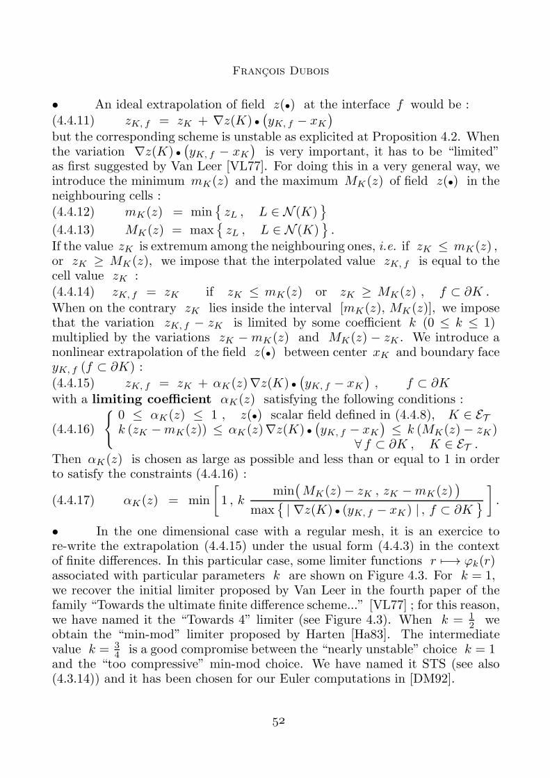
Francois Dubois
• An ideal extrapolation of field z(•) at the interface f would be :(4.4.11) zK, f = zK + ∇z(K) •
(yK, f − xK
)
but the corresponding scheme is unstable as explicited at Proposition 4.2. Whenthe variation ∇z(K) •
(yK, f − xK
)is very important, it has to be “limited”
as first suggested by Van Leer [VL77]. For doing this in a very general way, weintroduce the minimum mK(z) and the maximum MK(z) of field z(•) in theneighbouring cells :
(4.4.12) mK(z) = min{zL , L ∈ N (K)
}
(4.4.13) MK(z) = max{zL , L ∈ N (K)
}.
If the value zK is extremum among the neighbouring ones, i.e. if zK ≤ mK(z) ,or zK ≥ MK(z), we impose that the interpolated value zK, f is equal to thecell value zK :(4.4.14) zK, f = zK if zK ≤ mK(z) or zK ≥ MK(z) , f ⊂ ∂K .
When on the contrary zK lies inside the interval [mK(z), MK(z)], we imposethat the variation zK, f − zK is limited by some coefficient k (0 ≤ k ≤ 1)multiplied by the variations zK −mK(z) and MK(z) − zK . We introduce anonlinear extrapolation of the field z(•) between center xK and boundary faceyK, f (f ⊂ ∂K) :
(4.4.15) zK, f = zK + αK(z)∇z(K) •(yK, f − xK
), f ⊂ ∂K
with a limiting coefficient αK(z) satisfying the following conditions :
(4.4.16)
{0 ≤ αK(z) ≤ 1 , z(•) scalar field defined in (4.4.8), K ∈ ETk (zK −mK(z)) ≤ αK(z)∇z(K) •
(yK, f − xK
)≤ k (MK(z)− zK)
∀ f ⊂ ∂K , K ∈ ET .Then αK(z) is chosen as large as possible and less than or equal to 1 in orderto satisfy the constraints (4.4.16) :
(4.4.17) αK(z) = min
[1 , k
min(MK(z)− zK , zK −mK(z)
)
max{| ∇z(K) • (yK, f − xK) | , f ⊂ ∂K
}].
• In the one dimensional case with a regular mesh, it is an exercice tore-write the extrapolation (4.4.15) under the usual form (4.4.3) in the contextof finite differences. In this particular case, some limiter functions r 7−→ ϕk(r)associated with particular parameters k are shown on Figure 4.3. For k = 1,we recover the initial limiter proposed by Van Leer in the fourth paper of thefamily “Towards the ultimate finite difference scheme...” [VL77] ; for this reason,we have named it the “Towards 4” limiter (see Figure 4.3). When k = 1
2 weobtain the “min-mod” limiter proposed by Harten [Ha83]. The intermediatevalue k = 3
4 is a good compromise between the “nearly unstable” choice k = 1and the “too compressive” min-mod choice. We have named it STS (see also(4.3.14)) and it has been chosen for our Euler computations in [DM92].
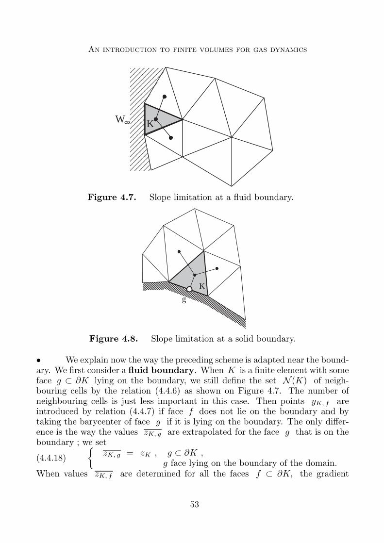
An introduction to finite volumes for gas dynamics
AAAAAAAAAAAAAAAAAAAAAAAAAAAAAAAA
W K∞
Figure 4.7. Slope limitation at a fluid boundary.
AAAAAAAAAAAAAAAAAAAAAAAAAAAAAAAAAAAAAAAAAAAAAAAAAAAAAAAAAAAA
K
g
Figure 4.8. Slope limitation at a solid boundary.
• We explain now the way the preceding scheme is adapted near the bound-ary. We first consider a fluid boundary. When K is a finite element with someface g ⊂ ∂K lying on the boundary, we still define the set N (K) of neigh-bouring cells by the relation (4.4.6) as shown on Figure 4.7. The number ofneighbouring cells is just less important in this case. Then points yK, f areintroduced by relation (4.4.7) if face f does not lie on the boundary and bytaking the barycenter of face g if it is lying on the boundary. The only differ-ence is the way the values zK, g are extrapolated for the face g that is on theboundary ; we set
(4.4.18)
{zK, g = zK , g ⊂ ∂K ,
g face lying on the boundary of the domain.When values zK, f are determined for all the faces f ⊂ ∂K, the gradient
Francois Dubois
∇z(K), the minimal mK(z) and maximal MK(z) values among the neigh-bouring cells are still determined with the relations (4.4.10), (4.4.12) and (4.4.13)respectively. The constraints (4.4.16) remain unchanged except that no limita-tion process is due to the faces lying on the boundary. In a precise way, weset :
(4.4.19)
αK(z) =
min
[1,
k min(MK(z)− zK , zK −mK(z)
)
max{|∇z(K)•(yK, f − xK) |, f ⊂ ∂K, Kr(f) ∈ N (K)
}].
Then the interpolated values zK, f for all the faces f ⊂ ∂K are again predictedwith the help of relation (4.4.15).• For a rigid wall, the limitation process is a little modified, as presentedat Figure 4.8. We first introduce the limit face g inside the set of neighbouringcells :
(4.4.20) N (K) =
{L∈ET , ∃f⊂∂K ∩ ∂L
}∪{
g∈FT , g ⊂ ∂K, g on the boundary}.
For the face(s) g ⊂ ∂K lying on the solid boundary, we determine preliminaryvalues zK, g by taking in consideration at this level the impenetrability bound-ary condition u •ng = 0. We introduce the two components nx
g and nyg of
the normal ng at the boundary and we set, in coherence with variables (4.4.8) :
(4.4.21)
ρK, g = ρKρK, g uK, g = ρK
(uK − (uK •ng)n
xg
)
ρK, g vK, g = ρK(vK − (uK •ng)n
yg
)
pK, g = pK .We consider also these values for the limitation algorithm. We define “externalvalues” zL for L=g and face g lying on the boundary as equal to the onesdefined in relation (4.4.21) :(4.4.22) zg ≡ zK, g , z(•) field defined in (4.4.21), g ⊂ ∂K on the boundary.Then the extrapolation algorithm that conducts to relation (4.4.15) for extrap-olated values zK, f is used as in the internal case.
4.5 Explicit Runge-Kutta integration with respect to time.• When all values zK, f are known for all control volumes K ∈ ET , allfaces f⊂K and all fields z(•) defined at relation (4.4.8), extrapolated statesWK, f are naturally defined by going back to the conservative variables. Thenwe introduce these states as arguments of the flux function Φ
(• , nf , •) and
obtain by this way a new system of ordinary differential equations :
(4.5.1) |K | dWK
dt+
∑
f⊂∂K
|f | Φ(WK, f , nf , WKr(f), f
)= 0 , K ∈ ET .
An introduction to finite volumes for gas dynamics
• The numerical integration of such kind of system is done with a Runge-Kutta scheme as presented in [CDV92]. We have used with success in [DM92] theHeun scheme of second order accuracy for discrete integration of (4.5.1) betweentime steps n∆t and (n+1)∆t :
(4.5.2)|K |∆t
(WK−Wn
K
)+∑
f⊂∂K
|f | Φ(Wn
K, f , nf , WnKr(f), f
)= 0 , K ∈ ET
(4.5.3)|K |∆t
( ˜WK−WK
)+∑
f⊂∂K
|f | Φ(WK, f , nf , WKr(f), f
)= 0 , K ∈ ET
(4.5.4) Wn+1K =
1
2
( ˜WK + Wn
K
), K ∈ ET .
5) References.[CDV92] D. Chargy, F. Dubois, J.P. Vila. Methodes numeriques pour le calcul
d’ecoulements compressibles, applications industrielles, cours de l’Institutpour la Promotion des Sciences de l’Ingenieur, Paris, septembre 1992.
[Ci78] P.G. Ciarlet. The Finite Element Method for Elliptic Problems, NorthHolland, Amsterdam, 1978.
[DM92] F. Dubois, O. Michaux. Solution of the Euler Equations Around a Dou-ble Ellipsoıdal Shape Using Unstructured Meshes and Including Real GasEffects, Workshop on Hypersonic Flows for Reentry Problems, (Desideri-Glowinski-Periaux Editors), Springer Verlag, vol. II, p. 358-373, 1992.
[DM96] F. Dubois, G. Mehlman. A non-parameterized entropy correctionfor Roe’s approximate Riemann solver, Numerische Mathematik, vol 73,p. 169-208, 1996.
[Du91] F. Dubois. Nonlinear Interpolation and Total Variation DiminishingSchemes, Third International Conference on Hyperbolic Problems, (Eng-quist-Gustafsson Editors), Chartwell-Bratt, p. 351-359, 1991. See alsohal-00493555.
[Du01] F. Dubois. Partial Riemann problem, Boundary conditions and gasdynamics, in Artificial Boundary Conditions, with Applications to Com-putational Fluid Dynamics Problems, (L. Halpern and L. Tourette Eds),Nova Science Publishers, p. 16-77, 2001. See also hal-00555600.
[FGH91] I. Faille, T. Gallouet, R. Herbin. Les Mathematiciens decouvrent lesVolumes Finis, Matapli, no 23, p. 37-48, octobre 1991.
[GR96] E. Godlewski, P.A. Raviart. Numerical Approximation of HyperbolicSystems of Conservation Laws, Applied Mathematical Sciences, vol. 118,Springer, New York, 1996.
Francois Dubois
[Go59] S.K. Godunov. A Difference Method for the Numerical Computationof Discontinuous Solutions of the Equations of Fluid Dynamics, Math.Sbornik, vol. 47, p. 271-290, 1959.
[GZIKP79] S.K. Godunov, A. Zabrodine, M. Ivanov, A. Kraiko, G. Prokopov.Resolution numerique des problemes multidimensionnels de la dynamiquedes gaz, Editions de Moscou, 1979.
[Ha83] A. Harten. High Resolution Schemes for Hyperbolic Conservation Laws,Journal of Computational Physics, vol. 49, p. 357-393, 1983.
[HLV83] A. Harten, P.D. Lax, B. Van Leer. On Upstream Differencing andGodunov-type Schemes for Hyperbolic Conservation Laws, SIAM Review,vol. 25, no 1, p. 35-61, January 1983.
[HGMW96] A. Hirschberg, J. Gilbert, R. Msallam, A.P.J. Wijnands. Shockwaves in trombones, J. Acoust. Soc. Am., vol. 99, no3, p. 1754-1758, 1996.
[Kr70] H.O. Kreiss. Initial Boundary Value Problems for Hyperbolic Systems,Comm. Pure Applied Math., vol. 23, p. 277-298, 1970.
[LL54] L. Landau, E. Lifchitz. Fluid Mechanics, Pergamon Press, 1954.
[MD99] R. Msallam, F. Dubois. Mathematical model for coupling a quasi-unidi-mensional perfect flow with an acoustic boundary layer, Research reportCNAM-IAT no 326/99, 1999. See also hal-00491417.
[Pa80] S.V. Patankar. Numerical Heat Transfer and Fluid Flow, Hemispherepublishing, 1980.
[Po88] M. Pollet. Methodes de calcul relatives aux interfaces missiles-propul-seurs, Internal report, Aerospatiale Les Mureaux, 1988.
[Roe81] P. Roe. Approximate Riemann Solvers, Parameter Vectors and Dif-ference Schemes, Journal of Computational Physics, vol. 43, p. 357-372,1981.
[Roe85] P. Roe. Some contributions to the Modelling of Discontinuous Flows, inLectures in Applied Mathematics, vol. 22, (Engquist, Osher, SommervilleEds), AMS, p. 163-193, 1985.
[RM67] R.D. Richtmyer, K.W. Morton. Difference Methods for Initial-ValueProblems, Interscience Publishing, J. Wiley & Sons, New York, 1967.
[VL77] B. Van Leer. Towards the Ultimate Conservative Difference SchemeIV. A New Approach to Numerical Convection, Journal of ComputationalPhysics, vol. 23, p. 276-299, 1977.
[VL79] B. Van Leer. Towards the Ultimate Conservative Difference Scheme V.A Second Order Sequel to Godunov’s Method, Journal of ComputationalPhysics, vol 32, n0 1, p. 101-136, 1979.