Marginal Likelihood Estimation with the

Cross-Entropy Method

Joshua C.C. Chan1 Eric Eisenstat2

1 Research School of Economics,

Australian National University, Australia2Faculty of Business Administration,

University of Bucharest and RIMIR, Romania

September 2012

Abstract

We consider an adaptive importance sampling approach to estimating the marginal likeli-hood, a quantity that is fundamental in Bayesian model comparison and Bayesian modelaveraging. This approach is motivated by the difficulty of obtaining an accurate estimatethrough existing algorithms that use Markov chain Monte Carlo (MCMC) draws, wherethe draws are typically costly to obtain and highly correlated in high-dimensional settings.In contrast, we use the cross-entropy (CE) method, a versatile adaptive Monte Carlo algo-rithm originally developed for rare-event simulation. The main advantage of the importancesampling approach is that random samples can be obtained from some convenient densitywith little additional costs. As we are generating independent draws instead of correlatedMCMC draws, the increase in simulation effort is much smaller should one wish to reducethe numerical standard error of the estimator. Moreover, the importance density derived viathe CE method is grounded in information theory, and therefore, is in a well-defined senseoptimal. We demonstrate the utility of the proposed approach by two empirical applicationsinvolving women’s labor market participation and U.S. macroeconomic time series. In bothapplications the proposed CE method compares favorably to existing estimators.

Keywords: importance sampling, model selection, probit, logit, time-varying parametervector autoregressive model, dynamic factor model

JEL classification codes: C11, C15, C32, C52

Acknowledgment: J. C. C. Chan’s research is supported by the Australian Research Council(Discovery Grant DP0985177 and DP0987170).

1 Introduction

This paper proposes a simple yet effective adaptive importance sampling approach to estimatingmarginal likelihoods that is readily implementable in a vast variety of econometric applications.The calculation of marginal likelihood, which is obtained by integrating the likelihood functionwith respect to the prior distribution, has attracted considerable interest in the Bayesian litera-ture due to its importance in Bayesian model comparison and Bayesian model averaging. In fact,there is a vast literature on estimating the normalizing constant of a given density by Markovchain Monte Carlo (MCMC) methods; see Gelfand and Dey (1994), Newton and Raftery (1994),Chib (1995), Gelman and Meng (1998), Chib and Jeliazkov (2001), Fruhwirth-Schnatter andWagner (2008) and Friel and Pettitt (2008), among many others. Although substantial progresshas been made from the statistics side in the last two decades, estimation of marginal likeli-hood, particularly in high-dimensional settings, remains a difficult problem. It continues to beespecially elusive in applied economic work due to the practical and computational burdenscharacterizing existing methods.

More specifically, not only do existing approaches often require nontrivial programming efforts,most involve using MCMC draws to compute certain Monte Carlo averages, which are then usedto derive an estimate of the normalizing constant. One major drawback of this approach is thatMCMC draws are typically costly to obtain. To compound the problem in high-dimensionalsettings, the draws are also often highly correlated. This is especially problematic, for example,when the researcher wishes to compare several similar models with a small dataset, wherethe marginal likelihoods under each model are expected to be similar, and therefore accurateestimates are required. For instance, to reduce the numerical standard error of an estimatorwith independent samples by a tenfold, one needs to increase the simulation effort by a factorof 100. With correlated MCMC draws, however, the increase in sample size could be muchlarger. In a typical situation in high-dimensional settings where the effective sample size is, say,0.02 (i.e., inefficiency factor equals 50), one needs to increase the simulation effort by 5000 toachieve the same reduction in the numerical standard error. In addition, since posterior drawsare usually costly to obtain, the computational effort required to discern the competing modelsmay be formidable.

In view of these drawbacks, we consider instead an adaptive importance sampling approachto estimating the marginal likelihood, where random samples can be obtained from some con-venient density with little additional costs. In addition, since we are generating independentdraws, the increase in simulation effort is much smaller should one wish to reduce the numeri-cal standard error of the estimator. The importance sampling approach is perhaps one of theearliest attempts to tackle the problem of marginal likelihood estimation; in fact, an early ap-plication of the importance sampling idea can be traced back to Geweke (1989). Of course,the trade-off in applying direct importance sampling is the complexity related to choosing animportance density from which to sample, and such a choice is not obvious in general. Typi-cally, for importance sampling to be successful, the importance density should at least satisfythe following three properties: (i) it is heavier-tailed than the target density, such that theresulting estimator has finite variance, (ii) it is practically simple to draw samples from, and(iii) it is easy to evaluate at any particular point in its support. Consequently, an ad hoc choiceof the importance density is likely to render the method impractical; yet, the choice of a “good”importance density is not always trivial.

2

Recently, Hoogerheide et al. (2007) present an innovative technique for estimation by fittingadaptively a mixture of Student-t distributions to the posterior density. Importance samplingis then used to obtain various quantities of interest, using the fitted mixture as an importancedensity. Ardia et al. (2010) later show that this approach allows an efficient and reliable esti-mation of marginal likelihood that performs well against existing methods. We build on thisline of research by proposing a methodological procedure for deriving an importance densitythat is in a well-defined sense optimal. Moreover, the proposed approach is generally applicableto a vast class of econometric models, including various high-dimensional latent data models(see Section 5). More specifically, we use the cross-entropy (CE) method, which is a versatileadaptive Monte Carlo algorithm originally developed for rare-event simulation by Rubinstein(1997). Since its inception, it has been applied to a diverse range of estimation problems, suchas network reliability estimation in telecommunications (Hui et al., 2005), efficient simulationof buffer overflow probabilities in queuing networks (de Boer et al., 2004), adaptive indepen-dence sampler design for MCMC methods (Keith et al., 2008), estimation of large portfolio lossprobabilities in credit risk models (Chan and Kroese, 2010), and other rare-event probabilityestimation problems involving light- and heavy-tailed random variables (Kroese and Rubinstein,2004; Asmussen et al., 2005). A recent review of the CE method and its applications can befound in Kroese (2010), and a book-length treatment is given in Rubinstein and Kroese (2004).

The CE method for importance sampling involves the following fundamental insights. First,for marginal likelihood estimation there exists an importance density that gives a zero-varianceestimator.1 In fact, if we use the posterior density as the importance density, then the associatedimportance sampling estimator has zero variance. Clearly, while in principle the posteriordensity gives the best estimator possible, it cannot be used in practice as its normalizing constantis the very unknown quantity we seek to estimate. On the other hand, a computationallytractable density that is “close” to the posterior density should be a good candidate, in the sensethat its associated estimator has a small variance. The CE method for importance samplingseeks to locate within a given parametric family the importance density that is the “closest” tothe zero-variance importance density, using the Kullback-Leibler divergence, or the cross-entropydistance as a measure of closeness between the two densities. As long as the parametric familyembodies the properties of convenient density evaluation and sample generation, the resultingdensity will typically yield an efficient and straightforward importance sampling algorithm.

From a statistics perspective, therefore, estimating the marginal likelihood by the CE methodproposed here is attractive because it inherits the well-known properties of importance sam-pling estimation. Moreover, employing an information-theoretic criterion for optimality is bothconceptually and practically appealing to economists. Indeed, information theory presents afamiliar approach in contemporary econometrics. For example, Zellner (1991) showed that min-imizing the Jeffreys-Kullback-Leibler distance between input information and output informa-tion in the process of learning from data leads to exactly the Bayes’ Rule upon which Bayesianinference is founded. Moreover, applying Bayes’ Rule results in the equivalence between inputinformation and output information such that Bayesian information processing is 100% efficient.Another important application of information theory in econometrics is formalized as maximumentropy econometrics (Golan et al., 1996) where emphasis is placed on efficiently extracting in-formation from the data with minimal a priori assumptions about the data-generating process.In this framework, rather than specifying and estimating a parametric likelihood function, the

1More generally, zero-variance importance distributions exist for estimation problems of the form EH(X),where H is a positive function.

3

researcher instead estimates an empirical distribution composed of a set of weights assigned tothe data points. To choose one of the infinitely many possible sets of weights, entropy is used toestablish the information-theoretic criterion that is minimized subject to the observed samplemoments. Maasoumi (1993) and Golan (2008) provide comprehensive overviews of informationtheory applications in econometrics. Tools offered by information theory have also been em-ployed (dating back to Arrow, 1970; Marschak, 1971) by economists in the theoretical modelingof risk and uncertainty.

On the practical side, it turns out that deriving the importance density by minimizing its cross-entropy distance to the posterior amounts to an exercise identical to likelihood maximization.Finally, we note that although the proposed approach also requires MCMC draws for obtainingthe optimal importance density, the number of draws needed is typically small (a few thousandsor less). In consequence, one obtains a marginal likelihood estimator that is relatively simpleto implement and does not require auxiliary reduced-run simulations in a wide variety of ap-plications. In addition, the proposed approach leads to a straightforward procedure to performprior sensitivity analysis without the need to have multiple MCMC runs. This is important asthe value of the marginal likelihood is often sensitive to the prior specification. It is thereforesensible to investigate if the conclusions based on the marginal likelihood criterion are robustunder different, yet reasonable, priors.

Despite their marked importance, model comparison and prior sensitivity analysis are oftenomitted in applied econometric work due to the programming and computational complexi-ties characterizing the existing methods for computing marginal likelihoods. The CE methodaims to overcome this by providing a more accessible methodology to applied economists with-out sacrificing effectiveness: as demonstrated by the empirical examples of Section 5, the CEmethod generally compares favorably with the most popular existing methods — and quiteoften provides substantial gains — in terms of computational efficiency.

The rest of this article is organized as follows. We first review the problem of estimating themarginal likelihood in Section 2, which is of importance in Bayesian econometrics and statistics.We then discuss two practical adaptive importance sampling approaches to tackle the problemin Section 3: the variance minimization (VM) and cross-entropy (CE) methods, with particularfocus on the latter. We then discuss in Section 4 a straightforward procedure to perform aprior sensitivity analysis via the proposed approach without having multiple MCMC runs. InSection 5 we present two empirical examples to demonstrate the utility and effectiveness of theproposed approach. The first example involves women’s labor market participation. There wecompare three different binary response models in order to find the one that best fits the data.The second example considers three popular vector autoregressive (VAR) models to analyze theinterdependence and structural stability of four U.S. macroeconomic time series: GDP growth,inflation, unemployment rate and interest rate.

2 Marginal Likelihood Estimation

To set the stage, consider the problem of comparing a collection of models M1, . . . ,MK. Eachmodel Mk is formally defined by a likelihood function p(y |θk,Mk) and a prior on the model-specific parameter vector θk denoted as p(θk |Mk). A popular criterion to compare between

4

models Mi and Mj is the posterior odds ratio between the two models:

POij ≡p(Mi |y)p(Mj |y)

=p(Mi)

p(Mj)× p(y |Mi)

p(y |Mj),

where p(Mk |y) is the posterior model probability of model Mk and

p(y |Mk) =

∫p(y |θk,Mk)p(θk |Mk)dθk

is the marginal likelihood under model Mk. The ratio p(y |Mi)/p(y |Mj) is often referred to asthe Bayes factor in favor of model Mi against model Mj . If both models are equally probable apriori, i.e., p(Mi) = p(Mj), the posterior odds ratio between the two models is then equal to theBayes factor. In addition, if we assume that the set of models under consideration is exhaustive,i.e.,

∑Kk=1

p(Mk |y) = 1, we can use the posterior odds ratios to obtain the posterior modelprobabilities. Specifically, it is easy to check that

p(Mi |y) =

1 +

K∑

k 6=i

POki

−1

.

For a more detailed discussion of the marginal likelihood and its role in Bayesian model com-parison and model averaging, see Gelman et al. (2003) and Koop (2003).

For moderately high-dimensional problems, analytic calculation of the marginal likelihood is al-most never possible. But with the advent of the Markov chain Monte Carlo methods, substantialprogress has been made to estimate this quantity using simulation methods. For notational con-venience, we suppress the model index from here onwards and write the marginal likelihood asp(y). There are many different approaches to estimate p(y) via MCMC methods, and here wemention two popular ones. Gelfand and Dey (1994) first realize that for any probability densityfunction f with support contained in the support of the posterior density, one has

E

[f(θ)

p(θ)p(y |θ)

∣∣∣∣ y]

=

∫f(θ)

p(θ)p(y |θ)p(θ |y)dθ

=

∫f(θ)

p(θ)p(y |θ)p(θ)p(y |θ)

p(y)dθ = p(y)−1. (1)

Therefore, they propose the following estimator for p(y):

pGD(y) =

1

L

L∑

l=1

f(θl)

p(y |θl)p(θl)

−1

, (2)

where θ1, . . . ,θL are posterior draws. Even though the equality in (1) holds for any densityfunction f , the estimator pGD(y) is biased, i.e., E[pGD(y)] 6= p(y) in general. Moreover, itsaccuracy depends crucially on the choice of the tuning function f . In view of this, Geweke (1999)proposes choosing f to be a normal approximation to the posterior density with a tail truncationdetermined by asymptotic arguments. We note in passing that the CE method described inthis paper may be easily adapted to provide an alternative to the tuning function suggestedin Geweke (1999). However, the resulting estimator pGD(y) would nevertheless be based oncorrelated MCMC draws from the posterior distribution, rather than truly independent draws

5

from the importance density, thereby still embodying a disadvantage relative to importancesampling algorithm we propose.

Another approach to computing the marginal likelihood, which is due to Chib (1995), does notrequire a tuning function. Indeed, the principal motivation for this approach is that “good”tuning functions are often difficult to find. To proceed, note that the marginal likelihood canbe written as

p(y) =p(y |θ)p(θ)p(θ |y) .

Hence, a natural estimator for p(y) is the quantity (written in logarithmic scale)

log p(y) = log p(y |θ∗) + log p(θ∗)− log p(θ∗ |y)

where θ∗ is any point in the support of the posterior distribution. In practice, it is often chosento be some “high density” point such as the posterior mean or mode. The only unknownquantity is the posterior ordinate p(θ∗ |y), which may be estimated by Monte Carlo methods.In particular, if posterior draws are obtained via the Gibbs sampler — i.e., when all the fullconditional distributions are known — then p(θ∗ |y) can be estimated by sampling draws from aseries of suitably designed Gibbs samplers, the so-called reduced runs. This approach, however,requires complete knowledge of all conditional distributions in the Gibbs scheme, which greatlyrestricts its applicability in practice. To overcome this limitation, Chib and Jeliazkov (2001)extend the basic approach to include cases when the full conditional distributions are intractableand Metropolis-Hastings steps are required. However, implementation of these extensions areconsiderably more involved, especially for computing numerical standard errors of marginallikelihood estimates. In addition, like the estimator of Gelfand and Dey (1994), the Chib’sestimator is also biased. There are many other approaches to marginal likelihood estimation,and we refer interested readers to the articles Han and Carlin (2001) and Friel and Pettitt (2008)for a more comprehensive review.

3 The Proposed Cross-Entropy Estimator

3.1 Importance Sampling and the Cross-Entropy Method

The basic idea of importance sampling — a fundamental Monte Carlo approach to estimatingthe expected value of an arbitrary function of random variables — is to bias the samplingdistribution in such a way that more “important values” are generated in the simulation. Thesimulation output is then weighted to correct for the use of the biased distribution to give anunbiased estimator. Specifically, to estimate the marginal likelihood p(y) =

∫p(y |θ)p(θ)dθ,

we consider the following importance sampling estimator:

pIS(y) =1

N

N∑

n=1

p(y |θn)p(θn)

g(θn), (3)

where θ1, . . . ,θN are independent draws obtained from the importance density g(·) that domi-nates p(y | ·)p(·), i.e., g(x) = 0 ⇒ p(y |x)p(x) = 0. Although the estimator in (3) is unbiased andconsistent for any such g, the performance of the estimator, particularly its variance, depends

6

critically on the choice of the importance density. In what follows, we apply the cross-entropy(CE) method, which establishes a well-defined criterion for the optimal choice of g, and gen-erates a straightforward procedure to derive the optimal importance density. The CE methodderives its name from the cross-entropy or Kullback-Leibler divergence — a fundamental con-cept in modern information theory. Textbook treatments of the CE method can be found inRubinstein and Kroese (2004) and Kroese et al. (2011, ch. 13); a recent survey of entropy andinformation-theoretic methods in econometrics is given in Golan (2008).

As previously discussed, the principal motivation of the CE approach is the fact that there existsan importance density that gives a zero variance estimator. That is, if we use the posteriordensity as the importance density, i.e., g(θ) = p(θ |y) = p(y |θ)p(θ)/p(y), then the associatedimportance sampling estimator (3) has zero variance:

pIS(y) =1

N

N∑

n=1

p(y |θn)p(θn)

g(θn)=

1

N

N∑

n=1

p(θn)p(y |θn)

p(θn)p(y |θn)/p(y)= p(y),

and we need to produce only N = 1 sample. For later reference we denote this zero-varianceimportance density as g∗. Although in principle g∗ gives the best possible estimator for p(y),it cannot be used in practice because the normalization constant of the density depends on themarginal likelihood, which is exactly the quantity one wishes to estimate. However, this suggestsa practical approach to obtain an optimal importance density. Intuitively, if one chooses g “closeenough” to g∗ so that both behave similarly, the resulting importance sampling estimator shouldhave reasonable accuracy. Hence, our goal is to locate a convenient density that is in a well-defined sense “close” to g∗. To this end, consider a parametric family F = f(θ;v) indexedby some parameter vector v within which we locate the importance density. We will shortlydiscuss various considerations in choosing such a family; for the moment we assume that Fis given. Now, we wish to find the density f(θ;v∗) ∈ F such that it is the “closest” to g∗.We consider two popular directed divergence measures of densities, which correspond to thevariance minimization (VM) and cross-entropy methods (CE). Let h1 and h2 be two probabilitydensity functions. The Pearson χ2 measure between h1 and h2 is defined as:

D2(h1, h2) =1

2

(∫h1(x)

2

h2(x)dx− 1

).

Since every density in F can be represented as f(·;v) for some v, the problem of obtaining theoptimal importance density now reduces to the following parametric minimization problem:

v∗vm = argmin

v

D2(g∗, f(·;v)).

Note that the value that minimizes any affine transformation of D2(g∗, f(·;v)) also minimizes

D2(g∗, f(·;v)) itself. Hence, we also have

v∗vm = argmin

v

p(y)2[2D2(g∗, f(·;v)) + 1] = argmin

v

∫p(y |θ)2p(θ)2

f(θ;v)dθ. (4)

From this it can be shown that minimizing the Pearson χ2 measure is the same as minimizingthe variance of the associated importance sampling estimator. In other words, f(θ;vvm) givesthe minimum variance estimator within the parametric class F . For this reason, this procedureis termed the variance minimization method. For a more detailed discussion of the Pearson χ2

measure and its applications, we refer the readers to Botev and Kroese (2011).

7

In practice, the optimization problem in (4) is often difficult to solve analytically. Instead, weconsider its stochastic counterpart:

vvm = argminv

1

L

L∑

l=1

p(y |θl)p(θl)

f(θl;v), (5)

where θ1, . . . ,θL are draws obtained from the posterior density p(θ |y) ∝ p(y |θ)p(θ). Notethat the optimization problem in (5) is equivalent to solving the following equation

1

L

L∑

l=1

p(y |θl)p(θl)

f(θl;v)∇v log f(θl;v) = 0, (6)

where ∇v is the gradient operator, which can be solved by various root-finding algorithms. TheVM method is summarized as follows:

Algorithm 1. VM Algorithm for Marginal Likelihood Estimation

1. Obtain a sample θ1, . . . ,θL from the posterior density g∗(θ) = p(θ |y) ∝ p(y |θ)p(θ) andfind the solution to (5) or equivalently (6), which is denoted as v∗

vm.

2. Generate a random sample θ1, . . . ,θN from the density f(·; v∗vm) and estimate p(y) via

importance sampling, as in (3).

One potential problem with the VM method is that in high-dimensional settings, the optimiza-tion problem in (5) or (6) might be difficult to solve. This motivates the consideration of a moreconvenient measure of “distance” between densities that leads to straightforward optimizationroutines in obtaining the optimal importance density. Let h1 and h2 be two probability den-sity functions. The Kullback-Leibler divergence, or cross-entropy distance between h1 and h2 isdefined as follows:

D1(h1, h2) =

∫h1(x) log

h1(x)

h2(x)dx.

As before, given the cross-entropy distance and a parametric family F , we then locate thedensity f(·;v) ∈ F such that D1(g

∗, f(·;v)) is minimized:

v∗ce = argmin

v

D1(g∗, f(·;v))

= argminv

(∫g∗(θ) log g∗(θ)dθ − p(y)−1

∫p(y |θ)p(θ) log f(θ;v)dθ

),

where we used the fact that g∗(θ) = p(y |θ)p(θ)/p(y). Since the term∫g∗(θ) log g∗(θ)dθ does

not depend on v, solving the CE minimization problem is equivalent to finding

v∗ce = argmax

v

∫p(y |θ)p(θ) log f(θ;v)dθ. (7)

Once again, we consider the stochastic counterpart of (7):

v∗ce = argmax

v

1

L

L∑

l=1

log f(θl;v), (8)

8

where θ1, . . . ,θL are draws from the posterior density. In other words, v∗ce is exactly the

maximum likelihood estimate for v if we view f(θ;v) as the likelihood function with parametervector v and θ1, . . . ,θL an observed sample. Since finding the maximum likelihood estimator(MLE) is a very well understood problem, solving (8) is typically easy. We summarize the CEmethod as below:

Algorithm 2. CE Algorithm for Marginal Likelihood Estimation

1. Obtain a sample θ1, . . . ,θL from the posterior density g∗(θ) = p(θ |y) ∝ p(y |θ)p(θ) andfind the solution to (8), which is denoted as v∗

ce.

2. Generate a random sample θ1, . . . ,θN from the density f(·; v∗ce) and estimate p(y) via

importance sampling, as in (3).

3.2 Choice of the Parametric Family F

We now discuss various considerations in choosing the parametric family F . First of all, it isobvious that it should be easy to generate random samples from any members of F ; otherwiseit would defeat the purpose of the proposed approach. This requirement, however, can beeasily met as efficient random variable generation is a very well-understood research area, andthere is a large variety of densities at our disposal from which samples can be readily obtained.Second, the computational burden of evaluating the density f(θ;v) at any point θ should besufficiently low, as this evaluation must be performed for each importance draw. To that end,most multivariate distributions that satisfy the first criterion of easy random sample generationare likewise straightforward to evaluate.

Additionally, the optimization problem (8) should be easily solved either analytically or nu-merically. Once again, this requirement can be easily met as solving (8) amounts to findingthe MLE if one views f(·;v) ∈ F as the likelihood for v. In fact, for the applications in thenext section, the optimization problem (8) can either be solved analytically, or reduced to aone-dimensional maximization problem. In addition, by choosing f(θ;v) as a product of densi-ties, e.g., f(θ;v) = f(θ1;v1) × · · · × f(θB ;vB), where θ = (θ1, . . . ,θB) and v = (v1, . . . ,vB),one can reduce the possibly high-dimensional maximization problem (8) into B low-dimensionalproblems, which can then be readily solved (albeit at some expense of “closeness” in the result-ing importance density to the posterior). It is likewise worth mentioning that the exponentialfamily provides a particularly appealing class of distributions in choosing F , since analyticalsolutions to (8) can often be found explicitly for such distributions (e.g., Rubinstein and Kroese,2004, p. 70).

A final, and slightly less obvious to handle consideration is that the importance density must beheavier-tailed than the posterior density in order for pIS(y) to have finite variance. Suppose thatthe posterior/likelihood is sufficiently peaked and well-behaved such that

∫p(y |θ)2p(θ)dθ < ∞,

then the crude Monte Carlo estimator, i.e., the importance sampling estimator associated withthe importance density g(θ) = p(θ), has finite variance. Hence, if we choose the family Fsuch that p(θ) ∈ F , then by construction the estimator associated with f(·;v∗

vm) has a smallervariance than the crude Monte Carlo estimator, and consequently its variance is also finite; seeProposition 2 in the next section for the exact statement, and Appendix B for the proof. Asfor the CE estimator (with importance density f(·;v∗

ce)), although the question of whether it

9

always provides variance reduction (compared to the crude Monte Carlo estimator) remainsopen in general, in a wide variety of applications the CE and VM estimators have very similarperformance. For example, in estimating buffer overflow probabilities, de Boer et al. (2004)find that the CE and VM estimators are essentially identical; in the settings of estimating theprobabilities that sums of independent random variables are larger than a given threshold, Chanet al. (2011) find that in all the cases studied both VM and CE methods prescribe the sameimportance sampling parameters. Furthermore, there are numerous heuristics to monitor thestability of the importance sampling estimator. For example, if the variance is indeed finite, weshould observe that an increase in the size of the importance sample by a factor of φ decreasesthe numerical standard error by a factor of

√φ. Since sampling from any member of F is by

construction inexpensive, this monitoring presents little additional difficulty. Consequently, ifone finds that additional sampling fails to decrease the numerical standard error of the marginallikelihood estimate, the parametric family should be appropriately expanded/modified. Weemphasize, however, that in our experience this complication is rarely present, and in suchexceptional cases when it does occur, the adjustments to F necessary to achieve the finitevariance property are often obvious.

3.3 Properties of the Proposed Estimators

In this section we document various desirable properties of the VM and CE estimators. Recallthat both are importance sampling estimators of the form given in (3), where the importancedensity g(θ) is f(·;v∗

vm) for the VM estimator and f(·;v∗ce) for the CE estimator. In particular,

one can easily show that both the VM and CE estimators are unbiased, in contrast to theestimators of Gelfand and Dey (1994) and Chib (1995), which are biased. Throughout thissection we assume:

Assumption 1. For any given data y, the likelihood function is bounded in the parametervector θ, i.e., there exists θ such that p(y |θ) 6 p(y | θ) for all θ in the parameter space.

Assumption 1 is a mild regularity condition that, for example, is necessary for the existenceof the maximum likelihood estimator. We need this assumption to show that the marginallikelihood p(y) is in fact finite.

Proposition 1. Suppose p(θ) is a proper prior and Assumption 1 holds. Further assume thatboth f(·;v∗

vm) and f(·;v∗ce) dominate p(y | ·)p(·), i.e., f(x;v∗

vm) = 0 ⇒ p(y |x)p(x) = 0. Thenthe VM and CE estimators are consistent and unbiased.

The proof is given in Appendix B. In addition, if the likelihood is sufficiently well-behaved, onecan further show that the variance of the VM estimator is finite, and therefore the central limittheorem applies to give an asymptotic distribution for the estimator.

Proposition 2. Suppose∫p(y |θ)2p(θ)dθ < ∞ and Assumption 1 holds. If the parametric

family F contains the prior density p(θ), then the variance of the VM estimator is finite.Furthermore, the VM estimator has an asymptotic normal distribution.

The reader is referred to Appendix B for a detailed proof.

10

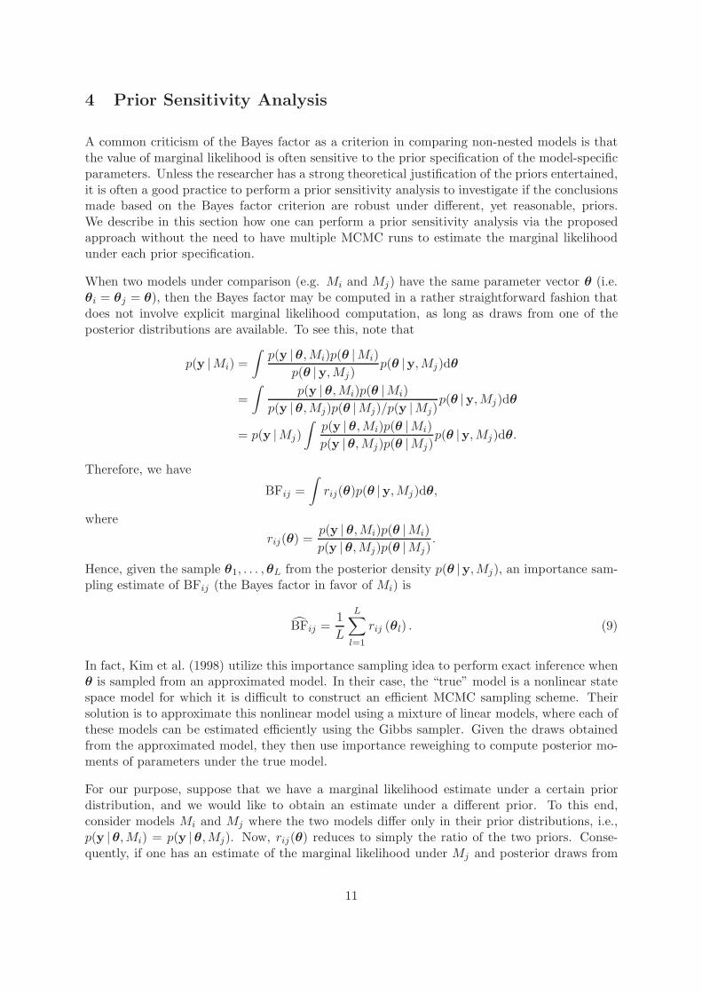
4 Prior Sensitivity Analysis

A common criticism of the Bayes factor as a criterion in comparing non-nested models is thatthe value of marginal likelihood is often sensitive to the prior specification of the model-specificparameters. Unless the researcher has a strong theoretical justification of the priors entertained,it is often a good practice to perform a prior sensitivity analysis to investigate if the conclusionsmade based on the Bayes factor criterion are robust under different, yet reasonable, priors.We describe in this section how one can perform a prior sensitivity analysis via the proposedapproach without the need to have multiple MCMC runs to estimate the marginal likelihoodunder each prior specification.

When two models under comparison (e.g. Mi and Mj) have the same parameter vector θ (i.e.θi = θj = θ), then the Bayes factor may be computed in a rather straightforward fashion thatdoes not involve explicit marginal likelihood computation, as long as draws from one of theposterior distributions are available. To see this, note that

p(y |Mi) =

∫p(y |θ,Mi)p(θ |Mi)

p(θ |y,Mj)p(θ |y,Mj)dθ

=

∫p(y |θ,Mi)p(θ |Mi)

p(y |θ,Mj)p(θ |Mj)/p(y |Mj)p(θ |y,Mj)dθ

= p(y |Mj)

∫p(y |θ,Mi)p(θ |Mi)

p(y |θ,Mj)p(θ |Mj)p(θ |y,Mj)dθ.

Therefore, we have

BFij =

∫rij(θ)p(θ |y,Mj)dθ,

where

rij(θ) =p(y |θ,Mi)p(θ |Mi)

p(y |θ,Mj)p(θ |Mj).

Hence, given the sample θ1, . . . ,θL from the posterior density p(θ |y,Mj), an importance sam-pling estimate of BFij (the Bayes factor in favor of Mi) is

BFij =1

L

L∑

l=1

rij (θl) . (9)

In fact, Kim et al. (1998) utilize this importance sampling idea to perform exact inference whenθ is sampled from an approximated model. In their case, the “true” model is a nonlinear statespace model for which it is difficult to construct an efficient MCMC sampling scheme. Theirsolution is to approximate this nonlinear model using a mixture of linear models, where each ofthese models can be estimated efficiently using the Gibbs sampler. Given the draws obtainedfrom the approximated model, they then use importance reweighing to compute posterior mo-ments of parameters under the true model.

For our purpose, suppose that we have a marginal likelihood estimate under a certain priordistribution, and we would like to obtain an estimate under a different prior. To this end,consider models Mi and Mj where the two models differ only in their prior distributions, i.e.,p(y |θ,Mi) = p(y |θ,Mj). Now, rij(θ) reduces to simply the ratio of the two priors. Conse-quently, if one has an estimate of the marginal likelihood under Mj and posterior draws from

11

p(y |θ,Mj), one can obtain an estimate for the marginal likelihood under Mi via (9). However,it is readily observed that for the importance sampling estimator (9) to work well, it is crucialthat the variability of the ratio rij(θ) is small under the posterior distribution p(y |θ,Mj);otherwise, estimates of BFij might be driven by a select few realizations of θ, and hence, berendered rather unstable. In other words, this approach can only reasonably accommodatesubtle to moderate differences in prior specifications. For radical differences, they will needto be compared by computing marginal likelihoods p(y |Mi) and p(y |Mj), separately. Hence,the accurate computation of marginal likelihoods is of central concern in model comparisonexercises and related interests.

To that end, we note that the proposed importance sampling approach of Section 3 likewiseprovides a straightforward way to perform a prior sensitivity analysis without the need to havemultiple MCMC runs. In addition, unlike the approach in (9), it is robust across rather differentprior specifications, as long as the posterior distribution does not change drastically under thedifferent priors. To motivate the procedure, recall that the CE method consists of two steps:first, we obtain MCMC draws (under a certain prior) to locate the optimal importance density.Second, we generate independent draws from the importance density to give an estimate asin (3). Now suppose that we have posterior draws from p(θ |y,Mj), and wish to estimate themarginal likelihood p(y |Mi) with the corresponding prior p(θ |Mi). As shown previously, thezero-variance importance density for estimating p(y |Mi) is the posterior density p(θ |y,Mi).However, in many situations, even though the priors are very different under the two modelsMi and Mj, the corresponding posterior distributions are similar (e.g., when the sample size ismoderately large). In those cases, draws from p(θ |y,Mj) are a good representation of drawsfrom p(θ |y,Mi). Hence, we can simply use the MCMC draws from the former to obtain v∗

ce

as in (8), then deliver the importance sampling estimator (3) with the prior p(θ |Mi). In whatfollows, we demonstrate that this approach works well across quite different prior specifications,and further show that the numerical standard error of the importance sampling estimator hardlychanges.

5 Empirical Applications

In this section, we present two empirical examples to illustrate the proposed importance sam-pling approach for estimating the marginal likelihood. In each of these examples, the implemen-tation is straightforward, and the estimate is accurate even for relatively small sample sizes. Inthe first example we consider three binary response models for women’s labor market partici-pation with logit, probit and t links. Since the link function is often chosen out of conveniencerather than being based on modeling considerations, a formal model comparison exercise seemsappropriate to determine which model best fits the data. The second empirical example is con-cerned with the US post-war macroeconomic time-series data involving GDP growth, inflation,unemployment and interest rate. We fit three popular vector autoregressive (VAR) models andformally compare them.

12

5.1 Binary Response Models for Women’s Labor Market Participation

In the first application we analyze a dataset from Mroz (1987) that deals with the labor marketparticipation decision of 200 married women using three binary response models with logit,probit and t links. Eight covariates are used to explain the binary indicator of labor marketparticipation — a constant, non-wife income, number of years of education, years of experience,experience squared (divided by 100), age, number of children less than six years of age in thehousehold, and number of children older than six years of age in the household. The likelihoodfor each of the binary response models has the form

p(y |β) =200∏

i=1

pyii (1− pi)1−yi , (10)

where β is a k × 1 parameter vector, pi = F (x′iβ) is the probability that the ith subject will

participate in the labor market, F (·) is a cumulative distribution function (cdf), yi ∈ 0, 1 isthe binary outcome variable, and xi is the covariate vector of the ith subject in the sample.

For the binary logit model, the cdf F is assumed to be logistic: F (z) = (1 + e−z)−1; for thebinary probit model, F (z) = Φ(z), where Φ is the cdf of the standard normal distribution.Lastly, F is assumed to be the cdf of a standard t distribution with degree of freedom ν = 10in the t model.

5.1.1 The Priors and Marginal Likelihood Estimation

For each of the three models, we assume a multivariate normal prior for β: β ∼ N(β0,V0) withβ0 = 0. Since the three models imply different variances (π2/3 for the logit model, 1 for theprobit model, and ν/(ν − 2) for the t model), we scale the covariance matrix V0 accordinglyto ensure the same prior is assumed across models. Specifically, we set V0 = τI for the logitmodel, V0 = 3/π2 × τI for the probit model, and V0 = 3ν/(π2(ν − 2)) × τI for the t model.The form of the prior (multivariate normal) is chosen for computational convenience — it is aconjugate prior for both the probit and the t-link models — and is standard in the literature. Toinvestigate the effect of the hyperparameters of the prior, we include a prior sensitivity analysisover a set of reasonably weakly-informative priors (with τ = 5, 10, 100) in the subsequent modelcomparison exercise.

We locate the optimal importance density within the parametric family F = fN(β;b,B)indexed by (b,B), where fN(· ;µ,Σ) is the multivariate normal density with mean vector µ andcovariance matrix Σ. Let β1, . . . ,βN be the posterior draws from a given model. To obtainthe CE reference parameters (b, B) for the optimal importance density, we need to solve themaximization problem (8). It is easy to check that the solution is simply

b =1

N

N∑

i=1

βi, B =1

N

N∑

i=1

(βi − b)(βi − b)′. (11)

In this case, therefore, the somewhat “obvious” choice of importance density, i.e. multivariatenormal parameterized by the posterior mean and posterior variance, is justified as the optimalchoice among all possible multivariate normal distributions. That is, setting the mean and

13

variance at the respective posterior counterparts minimizes its cross-entropy distance to theposterior density. As it turns out, it also leads to a well-performing importance samplingalgorithm that generates efficient estimates of the marginal likelihood.

To demonstrate the latter, for each of the three models we obtain a sample of size L = 5000 fromthe posterior density under the prior variance τ = 10 after a burn-in period of 500 draws, andcompute b and B as in (11). Given the optimal importance density fN(β; b, B), we estimate themarginal likelihoods of the three models, each with three different prior variances (τ = 5, 10, 100)by the importance sampling estimator in (3). For the main importance sampling run, we setthe sample size to be N = 5000.

5.1.2 Empirical Results

The importance sampling estimates for the log marginal likelihoods of the binary logit, probitand t models, as well as their numerical standard errors, are given in Table 1. Since the datasetis relatively small (sample size 200), the estimated marginal likelihoods for the three modelsare similar. Therefore, it is important in this case for the numerical standard errors for theestimates to be small. Under the set of priors considered, the probit model seems to be favoredby the data. In fact, if one assumes that the three models are equally likely a priori, thenthe posterior probabilities for the logit, probit and t models are respectively about 25%, 45%and 30% under all three prior specifications. Hence, for this particular dataset, the data showsmoderate support for the probit model, while the logit and t models are more or less equallylikely.

Table 1: Log marginal likelihood (numerical standard error) for the logit, probit and t modelsfor various prior specifications.

logit probit t-link

τ = 5 −138.68(0.005) −138.13(0.004) −138.85(0.004)τ = 10 −141.24(0.004) −140.67(0.003) −141.08(0.003)τ = 100 −150.23(0.005) −149.64(0.004) −150.06(0.005)

We also report the model parameter estimates for the probit model for τ = 10 in Table 2,together with the posterior standard deviations and the probabilities that the parameters arepositive. All parameter estimates have signs that are consistent with economic theory. Forinstance, non-wife income, age and the number of children in the household have a negativeimpact on the probability that an average woman will participate in the labor market. Onthe other hand, education and experience both have a positive impact, though the impactof experience is diminishing (the impact is quadratic in years of experience). However, notethe large posterior standard errors for the coefficients associated with the variables experiencesquared and children older than six.

14

Table 2: Parameter posterior means, standard deviations, and probabilities being positive forthe probit model.

Covariate E(· |y)√

Var(· |y) P(· > 0 |y)Constant 0.282 0.832 0.631Non-wife income −0.012 0.009 0.085Education 0.113 0.046 0.995Experience 0.100 0.041 0.992Experience squared −0.074 0.147 0.292Age −0.049 0.014 0.001Children younger than six −0.811 0.222 0Children older than six −0.005 0.080 0.475

5.1.3 Comparison with Other Methods

We now compare the empirical performance of the proposed CE estimator with two otherpopular methods for estimating the marginal likelihood. The first is the estimator of Gelfandand Dey (1994) with the tuning function suggested in Geweke (1999) — more precisely, amultivariate normal density truncated to its 95% highest density region — and we call thisthe GD-G method. The second estimator is the the method of Chib (1995) (for Gibbs output)and Chib and Jeliazkov (2001) (for Metropolis-Hastings output), and we refer to this the CJmethod. We use each of the three methods to estimate the marginal likelihoods of the threebinary response models, and compare the methods in terms of computation time and numericalaccuracy. Implementation details are given as follows. For the CE method, we first use L = 2500MCMC draws to compute the optimal importance sampling density for each of the three models,and then sample N = 50000 draws from the density obtained for the main importance samplingrun. For both the GD-G and CJ methods, we use L = 50000 MCMC draws to estimate themarginal likelihood. But instead of one long chain, we run 10 parallel chains each of lengthL = 5000, so that the numerical standard errors of the estimates can be readily computed.2

It is worth noting the different factors affecting the computation times of the three methods.Since both the GD-G and CJ methods require a lot of MCMC draws, when those draws aremore costly to obtain (e.g., more costly in the t-link model than in the probit model), bothmethods tend to be slower. When reduced runs are required, as in the logit model, the CJmethod tends to be slower (the other two methods do not require reduced runs). Finally, whenthe evaluation of the (integrated) likelihood function is more costly (e.g., more costly in thet-link model than in the probit model), the GD-G and CE methods — both require numerousevaluations of the likelihood function — tend to be slower.

2More precisely, the numerical standard error is calculated as the sample standard deviation of the 10 estimatesdivided by

√

10.

15

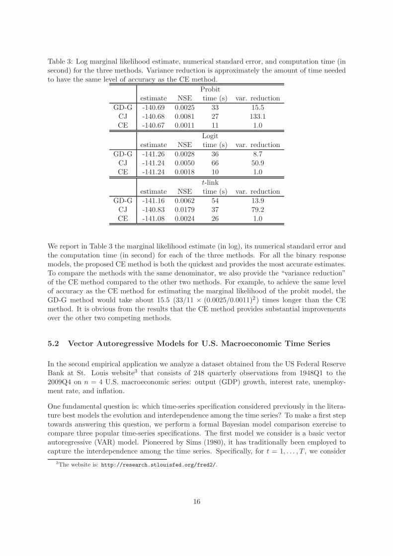
Table 3: Log marginal likelihood estimate, numerical standard error, and computation time (insecond) for the three methods. Variance reduction is approximately the amount of time neededto have the same level of accuracy as the CE method.

Probitestimate NSE time (s) var. reduction

GD-G -140.69 0.0025 33 15.5CJ -140.68 0.0081 27 133.1CE -140.67 0.0011 11 1.0

Logitestimate NSE time (s) var. reduction

GD-G -141.26 0.0028 36 8.7CJ -141.24 0.0050 66 50.9CE -141.24 0.0018 10 1.0

t-linkestimate NSE time (s) var. reduction

GD-G -141.16 0.0062 54 13.9CJ -140.83 0.0179 37 79.2CE -141.08 0.0024 26 1.0

We report in Table 3 the marginal likelihood estimate (in log), its numerical standard error andthe computation time (in second) for each of the three methods. For all the binary responsemodels, the proposed CE method is both the quickest and provides the most accurate estimates.To compare the methods with the same denominator, we also provide the “variance reduction”of the CE method compared to the other two methods. For example, to achieve the same levelof accuracy as the CE method for estimating the marginal likelihood of the probit model, theGD-G method would take about 15.5 (33/11 × (0.0025/0.0011)2 ) times longer than the CEmethod. It is obvious from the results that the CE method provides substantial improvementsover the other two competing methods.

5.2 Vector Autoregressive Models for U.S. Macroeconomic Time Series

In the second empirical application we analyze a dataset obtained from the US Federal ReserveBank at St. Louis website3 that consists of 248 quarterly observations from 1948Q1 to the2009Q4 on n = 4 U.S. macroeconomic series: output (GDP) growth, interest rate, unemploy-ment rate, and inflation.

One fundamental question is: which time-series specification considered previously in the litera-ture best models the evolution and interdependence among the time series? To make a first steptowards answering this question, we perform a formal Bayesian model comparison exercise tocompare three popular time-series specifications. The first model we consider is a basic vectorautoregressive (VAR) model. Pioneered by Sims (1980), it has traditionally been employed tocapture the interdependence among the time series. Specifically, for t = 1, . . . , T , we consider

3The website is: http://research.stlouisfed.org/fred2/.

16

the first-order VAR model

yt = µ+ Γyt−1 + εt, εt ∼ N(0,Ω), (12)

where yt is a vector containing measurements on the aforementioned n = 4 macroeconomicvariables (output growth, unemployment, income, and inflation), µ is an n× 1 vector of inter-cepts, Γ is an n × n matrix of parameters that governs the interdependence among the timeseries, and Ω is an unknown n × n positive definite covariance matrix. The analysis is per-formed conditionally on the initial data point and consequently our sample consists of T = 247observations.

For the purpose of estimation, (12) is rewritten in the form of a seemingly unrelated regression(SUR) model as follows:

yt = Xtβ + εt, (13)

whereXt = I⊗(1,y′t−1), β is a q×1 (q = n2+n) vector containing the corresponding parameters

from µ and Γ, ordered equation by equation, i.e., β = vec ((µ,Γ)′), and the vec(·) operatorstacks the columns of a matrix into a vector. Stacking the observations in (13) over t, we have

y = Xβ + ε, ε ∼ N(0, I ⊗Ω),

where

y =

y1

...yT

, X =

X1

...XT

, ε =

ε1...εT

.

Although the traditional VAR model is a popular specification for macroeconomic series, it is notflexible enough to accommodate potential structural instabilities in the times series. In view ofthis, in our second specification we extend the basic VAR model (12) by allowing the parametervector β to evolve over time in order to study the potential structural change of the time series.In particular, we consider the following first-order time-varying parameter vector autoregressive(TVP-VAR) model (e.g., Canova, 1992; Carter and Kohn, 1994; Koop and Korobilis, 2010):

yt = µt + Γtyt−1 + εt, εt ∼ N(0,Ω), (14)

where the parameters µt and Γt now have a subscript t to denote the time period. The evolutionof the parameter vector βt = vec ((µt,Γt)

′) for t = 2, . . . , T is governed by the evolution equation

βt = βt−1 + νt, (15)

with β1 ∼ N(0,D), where νt ∼ N(0,Σ), and Σ = diag(σ21, . . . , σ2

q ) is an unknown q×q diagonalmatrix. The transition equation (15) allows the elements of βt to evolve gradually over timeby penalizing large changes between successive values, thus a priori favoring the simple VARmodel with time-invariant parameters.

Another approach to extend the traditional VAR model (12) is the following dynamic factorVAR (DF-VAR) model (e.g., Bernanke et al., 2005; Koop and Korobilis, 2010):

yt = µ+ Γyt−1 +Aft + εt, εt ∼ N(0,Ω), (16)

17

where Ω = diag(ω21 , . . . , ω

2n) is a diagonal matrix, A is an n× 1 vector of factor loadings, and ft

is an unobserved factor that captures economy-wide macroeconomic volatility, which is assumedto evolve as

ft = γft−1 + ηt, ηt ∼ N(0, σ2

f ), (17)

for t = 2, . . . , T , and the initial factor f1 is distributed according to the stationary distributionf1 ∼ N(0, σ2

f/(1 − γ2)) with |γ| < 1. Since neither the factor loadings A nor the factorft isobserved, the scale and sign of A and ft are not individually identified becauseAft = (cA)(ft/c)for any c 6= 0. One popular identification assumption is to fixed the first element of A at 1, i.e.,A = (1,a′)′ and a is an (n − 1)× 1 vector of free parameters. With this assumption, both thesign and scale identification problems are resolved.

5.2.1 The Priors and Marginal Likelihood Estimation

In this subsection we describe the priors used in the three models and provide the implemen-tation details of the proposed importance sampling approach. Since the value of marginallikelihood in general is sensitive to the choice of priors, we maintain the same priors acrossmodels where appropriate. In addition, we consider a set of reasonable yet weakly-informativepriors in a prior sensitivity analysis to see how the marginal likelihood estimates are affectedby the choice of priors.

For the VAR model, the parameters are β and Ω with independent prior distributions: Ω ∼IW(ν0,S0) and β ∼ N(β0,Vβ), where IW(·, ·) is the inverse-Wishart distribution, ν0 = n +3,β0 = 0 and Vβ = 10× I. These are conjugate priors and are standard in the literature. ForS0 we consider two cases: S0 = I and S0 = 0.1×I. Standard results from the SUR model can beapplied to sample from the posterior density, e.g., see Koop (2003). To estimate the marginallikelihood of the model, we consider the parametric family F = fN(β;b,B)fIW(Ω; ν,S), wherefIW(·; ν,S) is the density of IW(ν,S). Given the posterior output βl,ΩlLl=1

, the optimal CE

reference parameters b and B can be obtained as in (11). As for ν and S, first note that

S−1 =1

νL

L∑

l=1

Ω−1

l .

Now by substituting S = S−1 into the density fIW(·; ν,S), ν can be obtained by any one-dimensional root-finding algorithm (e.g., Newton-Raphson method). Alternatively, simply fixingν = T also gives reasonable results. The former approach is the one we use for the empiricalexample.

For the TVP-VAR model, we assume that Ω ∼ IW(ν0,S0) and each diagonal element of Σfollows, independently, an inverse-gamma distribution: σ2

i ∼ IG(ν0i/2, S0i/2), for i = 1, . . . , q,with D = 10 × I, ν0 = n + 3, and ν0i = 6, S0i = 0.01 for i = 1, . . . , q. For S0, we consider twocases: S0 = I and S0 = 0.1 × I. Posterior inference is based on a recently proposed algorithmin Chan and Jeliazkov (2009), which we briefly describe in Appendix A. More importantlyfor our purpose, it also gives an efficient way to evaluate the integrated likelihood, defined asthe likelihood function marginal of the state vector β (see Appendix A for details). Hence,to compute the marginal likelihood of the TVP-VAR model, we can work with the integratedlikelihood f(y |Ω,Σ) rather than the complete-data likelihood f(y |β,Ω,Σ). This approachsubstantially reduces the variance of the importance sampling estimator as we analytically

18

“integrate out” β that consists of 247 βt’s, each of which is a 20-dimensional vector. Generally,in situations where the integrated likelihood f(y |θ) cannot be efficiently evaluated, one hasto work with the complete-data likelihood f(y | z,θ), where z is the latent variable vector.The proposed approach proceeds as before, with the optimal importance density f(θ, z; vce)constructed from the posterior draws. In this case, however, the variance of the associatedestimator is no smaller than the case where integrated likelihood f(y |θ) can be efficientlyevaluated. Now, to obtain the optimal importance density for the TVP-VAR model, we considerthe parametric family

F = fIW(Ω; ν,S)

q∏

i=1

fIG(σ2i ;mi, si).

The optimal CE parameters ν , S are obtained as in the previous case. Moreover, since theinverse-gamma density is a special case of the inverse-Wishart density, (mi, si), i = 1, . . . , q canbe obtained similarly.

Lastly, the priors for the parameters in the DF-VAR model are given as follows: β ∼ N(β0,Vβ),a ∼ N(a0,Va), and γ is distributed uniformly on the interval (−1, 1), with β0 = 0, Vβ = 10× I

and a0 = 0. For Va, we consider two cases Va = I and Va = 5 × I. In addition, eachdiagonal element ofΩ = diag(ω2

1, . . . , ω2

q ) follows, independently, an inverse-gamma distribution:ω2i ∼ IG(ν0i/2, S0i/2), for i = 1, . . . , q, and finally, σ2 ∼ IG(νf , Sf ), where νf = ν0i = 6,

Sf = S0i = 1. Posterior inference is based an efficient MCMC sampler discussed in Chanand Jeliazkov (2009). Specifically, instead of sequentially drawing from the full conditionals,we implement the following collapsed Markov sampler that substantially improves the mixingproperties and reduces the autocorrelation of the Markov chain:

Algorithm 3. Collapsed MCMC Sampling of β and A

1. [β |y,A,Ω, γ, σ2], which does not depend on f = (f1, . . . , fT )′

2. [a, f |y,β,Ω, γ, σ2], which is done using

(a) [a |y,β,Ω, γ, σ2], which does not depend on f

(b) [f |y,β,A,Ω, γ, σ2]

3. [Ω |y,β,A, f ]

4. [γ | f , σ2]

5. [σ2 | f , γ]

Again, the integrated likelihood is evaluated using the efficient algorithm described in Ap-pendix A. Now, to locate the optimal importance density, we consider the following parametricfamily

F =

fN(θ;bθ,Bθ)fN(γ; bγ , Bγ)fIG(σ

2;m, s)q∏

i=1

fIG(ω2i ;mi, si)

,

where θ = (β′,a′)′. Since the densities are either normal or inverse-gamma, the optimal CEreference parameters can be obtained exactly in the same way as before.

19

5.2.2 Empirical Results

Estimation results of the VAR, TVP-VAR and DF-VAR models for the U.S. macroeconomicdata are each based on a sample of L = 10000 MCMC draws after a burn-in of 500 draws, whichare obtained by the MCMC samplers described in Section 5.2.1. We first present in Figure 1 themain parameter of interest in the TVP-VAR model, β, the time-varying intercepts and VARcoefficients. The figure reveals that except for those coefficients in the unemployment equation,all the others exhibit considerable instability over the sampled periods, particularly the earlypart of the sample and the late 70s/early 80s. This suggests that the TVP-VAR model, whichallows for structural changes in the time series, seems to be a more suitable model for the U.S.data compared to the restrictive VAR model, which assumes constant coefficients over time.In fact, results from a formal exercise of Bayesian model comparison shows that this is indeedthe case (see below). Another point that is worth noting is that the impact of all the laggedmacroeconomic variables on GDP growth appears to have drifted towards zero in the latter partof the sample. This supports the contention of a “Great Moderation” in U.S. output growthvolatility that economic growth in the U.S. has become more stable over time due to lowerdependence on past outcomes.

1960 1980 2000−1

−0.5

0

0.5GDP growth equation

1960 1980 2000−0.4

−0.2

0

0.2

0.4

0.6Inflation rate equation

1960 1980 2000−0.5

0

0.5

1

1.5Unemployment equation

1960 1980 2000−1

0

1

2

3Interest rate equation

µt−1

GDPt−1

inflationt−1

unempt−1

interestt−1

Figure 1: Evolution of the parameters βt in the TVP-VAR model.

20

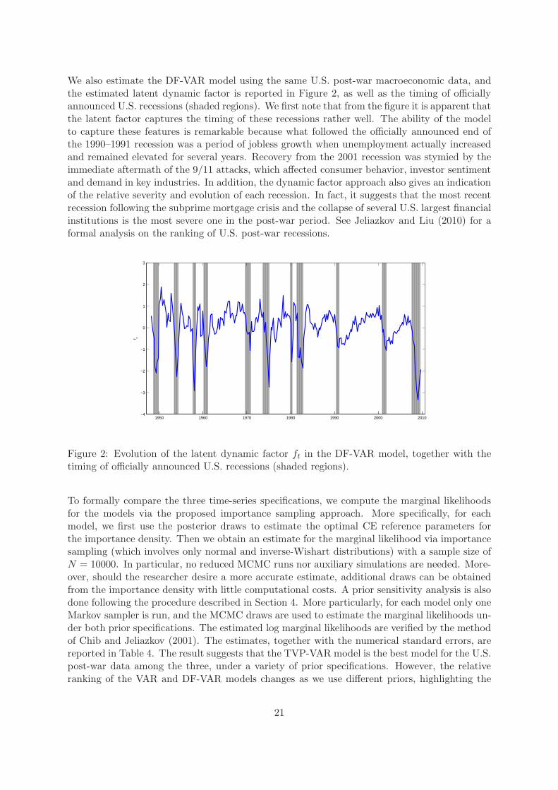
We also estimate the DF-VAR model using the same U.S. post-war macroeconomic data, andthe estimated latent dynamic factor is reported in Figure 2, as well as the timing of officiallyannounced U.S. recessions (shaded regions). We first note that from the figure it is apparent thatthe latent factor captures the timing of these recessions rather well. The ability of the modelto capture these features is remarkable because what followed the officially announced end ofthe 1990–1991 recession was a period of jobless growth when unemployment actually increasedand remained elevated for several years. Recovery from the 2001 recession was stymied by theimmediate aftermath of the 9/11 attacks, which affected consumer behavior, investor sentimentand demand in key industries. In addition, the dynamic factor approach also gives an indicationof the relative severity and evolution of each recession. In fact, it suggests that the most recentrecession following the subprime mortgage crisis and the collapse of several U.S. largest financialinstitutions is the most severe one in the post-war period. See Jeliazkov and Liu (2010) for aformal analysis on the ranking of U.S. post-war recessions.

1950 1960 1970 1980 1990 2000 2010

f t

−4

−3

−2

−1

0

1

2

3

Figure 2: Evolution of the latent dynamic factor ft in the DF-VAR model, together with thetiming of officially announced U.S. recessions (shaded regions).

To formally compare the three time-series specifications, we compute the marginal likelihoodsfor the models via the proposed importance sampling approach. More specifically, for eachmodel, we first use the posterior draws to estimate the optimal CE reference parameters forthe importance density. Then we obtain an estimate for the marginal likelihood via importancesampling (which involves only normal and inverse-Wishart distributions) with a sample size ofN = 10000. In particular, no reduced MCMC runs nor auxiliary simulations are needed. More-over, should the researcher desire a more accurate estimate, additional draws can be obtainedfrom the importance density with little computational costs. A prior sensitivity analysis is alsodone following the procedure described in Section 4. More particularly, for each model only oneMarkov sampler is run, and the MCMC draws are used to estimate the marginal likelihoods un-der both prior specifications. The estimated log marginal likelihoods are verified by the methodof Chib and Jeliazkov (2001). The estimates, together with the numerical standard errors, arereported in Table 4. The result suggests that the TVP-VAR model is the best model for the U.S.post-war data among the three, under a variety of prior specifications. However, the relativeranking of the VAR and DF-VAR models changes as we use different priors, highlighting the

21

importance of a prior sensitivity analysis in marginal likelihood estimation.

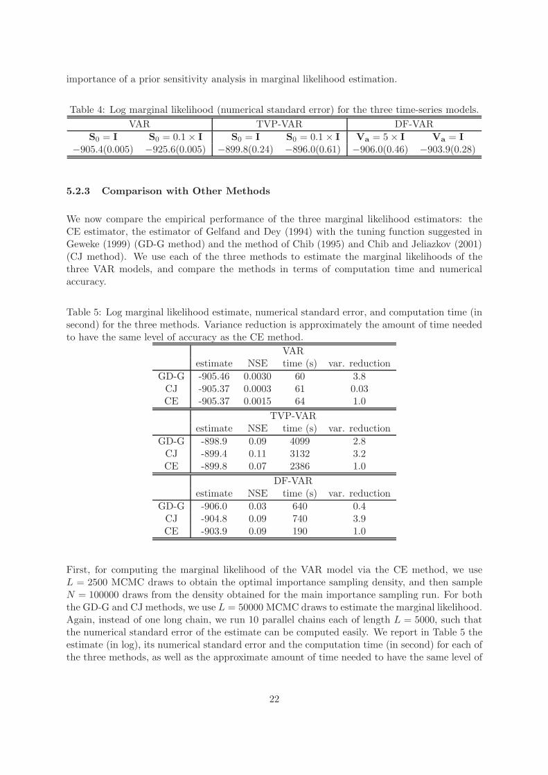
Table 4: Log marginal likelihood (numerical standard error) for the three time-series models.

VAR TVP-VAR DF-VAR

S0 = I S0 = 0.1× I S0 = I S0 = 0.1 × I Va = 5× I Va = I

−905.4(0.005) −925.6(0.005) −899.8(0.24) −896.0(0.61) −906.0(0.46) −903.9(0.28)

5.2.3 Comparison with Other Methods

We now compare the empirical performance of the three marginal likelihood estimators: theCE estimator, the estimator of Gelfand and Dey (1994) with the tuning function suggested inGeweke (1999) (GD-G method) and the method of Chib (1995) and Chib and Jeliazkov (2001)(CJ method). We use each of the three methods to estimate the marginal likelihoods of thethree VAR models, and compare the methods in terms of computation time and numericalaccuracy.

Table 5: Log marginal likelihood estimate, numerical standard error, and computation time (insecond) for the three methods. Variance reduction is approximately the amount of time neededto have the same level of accuracy as the CE method.

VARestimate NSE time (s) var. reduction

GD-G -905.46 0.0030 60 3.8CJ -905.37 0.0003 61 0.03CE -905.37 0.0015 64 1.0

TVP-VARestimate NSE time (s) var. reduction

GD-G -898.9 0.09 4099 2.8CJ -899.4 0.11 3132 3.2CE -899.8 0.07 2386 1.0

DF-VARestimate NSE time (s) var. reduction

GD-G -906.0 0.03 640 0.4CJ -904.8 0.09 740 3.9CE -903.9 0.09 190 1.0

First, for computing the marginal likelihood of the VAR model via the CE method, we useL = 2500 MCMC draws to obtain the optimal importance sampling density, and then sampleN = 100000 draws from the density obtained for the main importance sampling run. For boththe GD-G and CJ methods, we use L = 50000 MCMC draws to estimate the marginal likelihood.Again, instead of one long chain, we run 10 parallel chains each of length L = 5000, such thatthe numerical standard error of the estimate can be computed easily. We report in Table 5 theestimate (in log), its numerical standard error and the computation time (in second) for each ofthe three methods, as well as the approximate amount of time needed to have the same level of

22

accuracy as the CE method. For this relatively low-dimensional model, all three methods workvery well, and the CJ method gives the most accurate estimate per unit of computation time.

We then perform the same exercise for the TVP-VAR model. The CE method uses L = 5000MCMC draws for obtaining the optimal importance sampling density and N = 100000 draws forthe main importance sampling run; both the GD-G and CJ methods use L = 100000 MCMCdraws. Estimation of the marginal likelihood is much more time-consuming for this high-dimensional model: the GD-G, CJ and CE methods take respectively 68, 52 and 40 minutes.For the TVP-VAR model, the CE method is the fastest and most accurate. For instance, the CJmethod would need about 129 minutes to achieve the same level of accuracy as the CE method(which takes only 40 minutes).

Finally, for the DF-VAR model, the CE method uses L = 5000 MCMC draws and N = 100000draws from the importance density; both the GD-G and CJ methods use L = 100000 MCMCdraws. Although the CE method is the fastest, the GD-G method seems to provide the mostaccurate estimate given the same computation time. However, it is also worth noting that theGD-G estimate is slightly different from those obtained via the CJ and CE methods (takinginto account of the small numerical standard errors). Since both the CJ and GD-G methodsgive biased estimates, while the CE estimate is unbiased, this small discrepancy in the estimatesmight reflect a non-negligible bias in the GD-G estimate in this particular example.

6 Concluding Remarks

In this article we introduce the CE method to tackle an important problem in Bayesian econo-metrics and statistics, namely, the estimation of marginal likelihood. Although the problem iswell-studied and many approaches already exist, the proposed method has the merit of beingboth conceptually and computationally simple. In particular, it is essentially an importancesampling approach, with the choice of importance density guided by a methodology foundedon formal optimization by minimizing the cross-entropy distance to the posterior density (i.e.the intractable zero-variance importance density). Therefore, the importance density is cho-sen to systematically minimize the variance of the resulting estimate, yet random samples canbe obtained from it conveniently with negligible computational costs. Furthermore, since thedraws are independent by construction, the simulation effort is much less compared to otherapproaches should one wish to reduce the numerical standard error of the estimator. In the twoempirical applications studied, the CE method compares favorably to existing estimators.

Generally, this approach relies on the researcher designating a family of densities on which theCE-based optimization method is implemented to operate. For many applications, as demon-strated through two empirical examples in the text, this choice of distribution family is relativelystraightforward. Typically, it will be sufficient to match the chosen family with the class of priordistributions employed by the model. Regardless of the family chosen, however, the eventualoptimization over this collection, as prescribed by the CE approach, amounts to an exercisedirectly analogous to likelihood maximization.

This suggests, therefore, that when a particular choice of distribution family is inadequate,straightforward extensions are readily available. For example, it may be worthwhile to considerexpanding a family of multivariate normal distributions to one consisting of a mixture of mul-

23

tivariate normal distributions. Such a generalization presents little additional computationaldifficulties – multivariate normal mixture likelihoods, while no longer analytically tractable, areeasily maximized by Expectation-Maximization based techniques. To that end, an interestingand important extension of the algorithm presented in this paper would be one incorporatingthe automatic selection of the parametric family. We leave the latter open for future work.

Aside from the fact that following the CE approach leads to a simple, yet methodological con-struction of importance densities, the empirical examples discussed in Section 5 further illustratethe overall utility of implementing importance sampling in this way to estimate marginal likeli-hoods. In both cases, the proposed algorithm is not only fast and and easy to implement, butit also gives very accurate marginal likelihood estimates with a relatively small sample size.

Appendix A: Efficient Simulation of the Gaussian State Space

Models

In this appendix we present an efficient Markov sampler proposed in Chan and Jeliazkov (2009)for simulation and integrated likelihood estimation in state space models. We consider thefollowing linear Gaussian state space model:

yt = Xtβ +Gtηt + εt, (18)

ηt = Ztγ + Ftηt−1 + νt, (19)

for t = 1, . . . , T , where yt is an n×1 vector of observations, ηt is a q×1 latent state vector, (19)is initialized with η1 ∼ N(Z1γ,D), and

(εtνt

)∼ N

(0,

(Ω11 0

0 Ω22

)).

Equation (18) is often referred to as the measurement or observation equation, while (19) iscalled the transition or evolution equation. Define y = (y1, . . . ,yT ) and η = (η1, . . . ,ηT ), andlet θ represent the parameters in the state space model (i.e. β, γ, Gt, Ft, and the uniqueelements of Ω11, Ω22, and D). The covariates Xt and Zt are taken as given and will besuppressed in the conditioning sets below.

From (18)–(19) it is easily seen that the joint sampling density f(y |θ,η) is Gaussian. In fact,stacking (18)–(19) over the T time periods, we have

y = Xβ +Gη + ε,

where

X =

X1

...XT

, G =

G1

. . .

GT

, ε =

ε1...εT

,

with ε ∼ N(0, I ⊗Ω11). A change of variable from ε to y implies that

f(y |θ,η) = fN(y |Xβ +Gη, I⊗Ω11). (20)

24

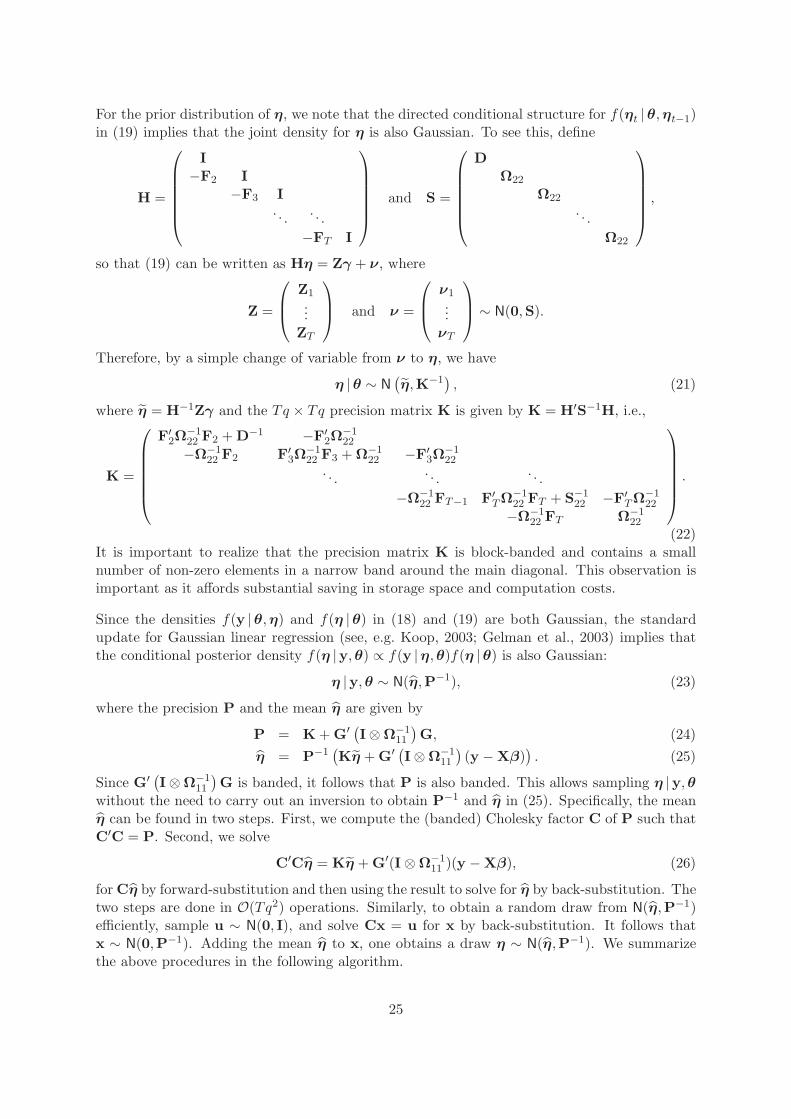
For the prior distribution of η, we note that the directed conditional structure for f(ηt |θ,ηt−1)in (19) implies that the joint density for η is also Gaussian. To see this, define

H =

I

−F2 I

−F3 I. . .

. . .

−FT I

and S =

D

Ω22

Ω22

. . .

Ω22

,

so that (19) can be written as Hη = Zγ + ν, where

Z =

Z1

...ZT

and ν =

ν1

...νT

∼ N(0,S).

Therefore, by a simple change of variable from ν to η, we have

η |θ ∼ N(η,K−1

), (21)

where η = H−1Zγ and the Tq × Tq precision matrix K is given by K = H′S−1H, i.e.,

K =

F′2Ω

−1

22F2 +D−1 −F′

2Ω−1

22

−Ω−1

22F2 F′

3Ω−1

22F3 +Ω−1

22−F′

3Ω−1

22

. . .. . .

. . .

−Ω−1

22FT−1 F′

TΩ−1

22FT + S−1

22−F′

TΩ−1

22

−Ω−1

22FT Ω−1

22

.

(22)It is important to realize that the precision matrix K is block-banded and contains a smallnumber of non-zero elements in a narrow band around the main diagonal. This observation isimportant as it affords substantial saving in storage space and computation costs.

Since the densities f(y |θ,η) and f(η |θ) in (18) and (19) are both Gaussian, the standardupdate for Gaussian linear regression (see, e.g. Koop, 2003; Gelman et al., 2003) implies thatthe conditional posterior density f(η |y,θ) ∝ f(y |η,θ)f(η |θ) is also Gaussian:

η |y,θ ∼ N(η,P−1), (23)

where the precision P and the mean η are given by

P = K+G′(I⊗Ω−1

11

)G, (24)

η = P−1(Kη +G′

(I⊗Ω−1

11

)(y −Xβ)

). (25)

Since G′(I⊗Ω−1

11

)G is banded, it follows that P is also banded. This allows sampling η |y,θ

without the need to carry out an inversion to obtain P−1 and η in (25). Specifically, the meanη can be found in two steps. First, we compute the (banded) Cholesky factor C of P such thatC′C = P. Second, we solve

C′Cη = Kη +G′(I ⊗Ω−1

11)(y −Xβ), (26)

forCη by forward-substitution and then using the result to solve for η by back-substitution. Thetwo steps are done in O(Tq2) operations. Similarly, to obtain a random draw from N(η,P−1)efficiently, sample u ∼ N(0, I), and solve Cx = u for x by back-substitution. It follows thatx ∼ N(0,P−1). Adding the mean η to x, one obtains a draw η ∼ N(η,P−1). We summarizethe above procedures in the following algorithm.

25

Algorithm 4. Efficient State Smoothing and Simulation

1. Compute P in (24) and obtain its Cholesky factor C such that P = C′C.

2. Smoothing: Solve (26) by forward- and back-substitution to obtain η.

3. Simulation: Sample u ∼ N(0, I), and solve Cx = u for x by back-substitution and takeη = η + x, so that η ∼ N(η,P−1).

Lastly, we describe an efficient method to evaluate the integrated likelihood f(y |θ), defined as

f(y |θ) =∫

f(y |θ,η)f(η |θ)dη, (27)

where f(y |θ,η) is the likelihood and f(η |θ) represents the prior. This quantity is often usedin likelihood evaluation for classical and Bayesian problems involving optimization and modelcomparison. Evaluating the integrated likelihood via the multivariate integration in (27) iscomputationally intensive and often impractical. However, the derivation of the full condi-tional density f(η|y,θ) discussed above provides a simple way to evaluate f(y |θ) withoutinvoking (27). Specifically, it follows from the Bayes’ theorem that integrated likelihood as

f(y |θ) = f(y |θ,η)f(η |θ)f(η |y,θ) , (28)

where f(η |y,θ) denotes the full conditional posterior density of η given (y,θ). Due to thebanded nature of the prior and posterior precision matrices (K and P, respectively), evaluationof the integrated likelihood f(y |θ) at the point θ can be done efficiently simply by evaluating theright-hand-side of (28) at a single point (θ,η). Note that the choice is arbitrary, in particular,the choice η = η eliminates the need to compute the exponential part of the density functionin the denominator density.

Appendix B: Proofs of Propositions

Proof of Proposition 1. We first show that the marginal likelihood p(y) is finite for any giveny. Using Assumption 1 and the fact that the prior is proper, we have

p(y) =

∫p(y |θ)p(θ)dθ 6 p(y | θ)

∫p(θ)dθ = p(y | θ) < ∞.

Now write the VM estimator as the the average of N iid copies of the random variable Zn:

pvm(y) =1

N

N∑

n=1

Zn,

where Zn = p(y |θn)p(θn)/f(θn;v∗vm) and θn ∼ f(θn;v

∗vm). It is easy to see that

EZn =

∫p(y |θn)p(θn)

f(θn;v∗vm)

f(θn;v∗vm)dθn =

∫p(y |θn)p(θn)dθn = p(y) < ∞.

26

Therefore, by the (weak) law of large number, pvm(y) converges in probability to p(y) asN → ∞. Next, note that

E [pvm(y)] = E

[1

N

N∑

n=1

Zn

]=

1

N

N∑

n=1

p(y) = p(y).

That is, the VM estimator is also unbiased.

The case for the CE estimator is similar. As before, write the CE estimator as the the averageof N iid copies of the random variable Wn:

pce(y) =1

N

N∑

n=1

Wn,

where Wn = p(y |θn)p(θn)/f(θn;v∗ce) and θn ∼ f(θn;v

∗ce). Then, we have

EWn =

∫p(y |θn)p(θn)

f(θn;v∗ce)

f(θn;v∗ce)dθn =

∫p(y |θn)p(θn)dθn = p(y) < ∞.

Since EWn = p(y) < ∞, by the (weak) law of large number, pce(y) converges in probability top(y) as N → ∞. Finally,

E [pce(y)] = E

[1

N

N∑

n=1

Wn

]=

1

N

N∑

n=1

p(y) = p(y).

Therefore, the CE estimator is also unbiased and consistent.

If the parametric family F contains the prior density p(·), then the variance of the VM estimatoris finite. Furthermore, the VM estimator has an asymptotic normal distribution.

Proof of Proposition 2. Let Z = p(y |θ)p(θ)/f(θ;v∗vm), where θ ∼ f(θ;v∗

vm). Then the VMestimator pvm(y) is simply the average of N independent copies of Z. We will first show thatthe second moment of Z, EZ2, is finite. By the definition of v∗

vm in (4) and the assumptionthat the prior density p(θ) is in the parametric family F , it follows that

EZ2 =

∫p(y |θ)2p(θ)2f(θ;v∗

vm)dθ 6

∫p(y |θ)2p(θ)2

p(θ)dθ =

∫p(y |θ)2p(θ)dθ < ∞.

Now, we have

Var(pvm(y)) =Var(Z)

N6

EZ2

N< ∞.

Since EZ = p(y) and σ2 ≡ Var(Z) < ∞, by the central limit theorem, we finally have

√N(pvm(y)− p(y))

d→N(0, σ2),

as N → ∞.

27

References

D. Ardia, N. Basturk, L. Hoogerheide, and H. K. van Dijk. A comparative study of MonteCarlo methods for efficient evaluation of marginal likelihood. Computational Statistics andData Analysis, 2010. In press.

K. J. Arrow. Essays in the Theory of Risk Bearing. North-Holland, Amsterdam, 1970.

S. Asmussen, R. Y. Rubinstein, and D. P. Kroese. Heavy tails, importance sampling and cross-entropy. Stochastic Models, 21:57–76, 2005.

B. Bernanke, J. Boivin, and P. S. Eliasz. Measuring the effects of monetary policy: A factor-augmented vector autoregressive (FAVAR) approach. The Quarterly Journal of Economics,120(1):387–422, 2005.

Z. I. Botev and D. P. Kroese. The generalized cross-entropy method, with applications toprobability density estimation. Methodology and Computing in Applied Probability, 13:1–27,2011.

F. Canova. Modelling and forecasting exchange rates with a Bayesian time-varying coefficientmodel. Journal of Economic Dynamics and Control, 17:233–262, 1992.

C. K. Carter and R. Kohn. On Gibbs sampling for state space models. Biometrika, 81:541–553,1994.

J. C. C. Chan and I. Jeliazkov. Efficient simulation and integrated likelihood estimation in statespace models. International Journal of Mathematical Modelling and Numerical Optimisation,1:101–120, 2009.

J. C. C. Chan and D. P. Kroese. Efficient estimation of large portfolio loss probabilities int-copula models. European Journal of Operational Research, 205:361–367, 2010.

J. C. C. Chan, P. W. Glynn, and D. P. Kroese. A comparison of cross-entropy and varianceminimization strategies. Journal of Applied Probability, 48A:183–194, 2011.

S. Chib. Marginal likelihood from the Gibbs output. Journal of the American StatisticalAssociation, 90:1313–1321, 1995.

S. Chib and I. Jeliazkov. Marginal likelihood from the Metropolis-Hastings output. Journal ofthe American Statistical Association, 96:270–281, 2001.

P. T. de Boer, D. P. Kroese, and R. Y. Rubinstein. A fast cross-entropy method for estimatingbuffer overflows in queueing networks. Management Science, 50:883–895, 2004.

N. Friel and A. N. Pettitt. Marginal likelihood estimation via power posteriors. Journal RoyalStatistical Society Series B, 70:589–607, 2008.

S. Fruhwirth-Schnatter and Helga Wagner. Marginal likelihoods for non-Gaussian models usingauxiliary mixture sampling. Computational Statistics and Data Analysis, 52(10):4608 – 4624,2008.

A. E. Gelfand and D. K. Dey. Bayesian model choice: Asymptotics and exact calculations.Journal of the Royal Statistical Society Series B, 56(3):501–514, 1994.

28

A. Gelman and X. Meng. Simulating normalizing constants: From importance sampling tobridge sampling to path sampling. Statistical Science, 13:163–185, 1998.

A. Gelman, J. B. Carlin, H. S. Stern, and D. B. Rubin. Bayesian Data Analysis. Chapman &Hall, New York, second edition, 2003.

J. Geweke. Exact predictive densities for linear models with ARCH disturbances. Journal ofEconometrics, 40(1):63 – 86, 1989.

J. Geweke. Using simulation methods for Bayesian econometric models: inference, development,and communication. Econometric Reviews, 18(1):1–73, 1999.

A. Golan. Information and entropy econometrics – a review and synthesis. Foundations andTrends in Econometrics, 2(1-2):1–145, 2008.

A. Golan, G. G. Judge, and D. Miller. Maximum Entropy Econometrics: Robust Estimationwith Limited Data. Wiley, New York, 1996.

C. Han and B. P. Carlin. Markov chain Monte Carlo methods for computing Bayes factors: acomparative review. Journal of the American Statistical Association, 96:1122–1132, 2001.

L. F. Hoogerheide, J. F. Kaashoek, and H. K. van Dijk. On the shape of posterior densities andcredible sets in instrumental variable regression models with reduced rank: An application offlexible sampling methods using neural networks. Journal of Econometrics, 139(1):154–180,2007.

K-P. Hui, N. Bean, M. Kraetzl, and D. P. Kroese. The cross-entropy method for networkreliability estimation. Annals of Operations Research, 134:101–118, 2005.

I. Jeliazkov and R. Liu. A model-based ranking of U.S. recessions. Economics Bulletin, 30(3):2289–2296, 2010.

J. M. Keith, D. P. Kroese, and G. Y. Sofronov. Adaptive independence samplers. Statistics andComputing, 18:409–420, 2008.

S. Kim, N. Shephard, and S. Chib. Stochastic volatility: Likelihood inference and comparisonwith ARCH models. Review of Economic Studies, 65(3):361–393, 1998.

G. Koop. Bayesian Econometrics. Wiley & Sons, New York, 2003.

G. Koop and D. Korobilis. Bayesian multivariate time series methods for empirical macroeco-nomics. Foundations and Trends in Econometrics, 3(4):267–358, 2010.

D. P. Kroese. The cross-entropy method. In James J. Cochran, Louis A. Cox, Pinar Keskinocak,Jeffrey P. Kharoufeh, and J. Cole Smith, editors, Wiley Encyclopedia of Operations Researchand Management Science. Wiley & Sons, New York, 2010.

D. P. Kroese and R. Y. Rubinstein. The transform likelihood ratio method for rare eventsimulation with heavy tails. Queueing Systems, 46:317–351, 2004.

D. P. Kroese, T. Taimre, and Z. I. Botev. Handbook of Monte Carlo Methods. John Wiley &Sons, New York, 2011.

29

E. Maasoumi. A compendium to information theory in economics and econometrics. Econo-metric Reviews, 12:137–181, 1993.

J. Marschak. Economics of information systems. Journal of the American Statistical Association,66:192–219, 1971.

T. A. Mroz. The sensitivity of an empirical model of married women’s hours of work to economicand statistical assumptions. Econometrica, 55:765–799, 1987.

M. A. Newton and A. E. Raftery. Approximate Bayesian inference with the weighted likelihoodbootstrap. Journal of the Royal Statistical Society Series B, 56:3–48, 1994.

R. Y. Rubinstein. Optimization of computer simulation models with rare events. EuropeanJournal of Operational Research, 99:89–112, 1997.

R. Y. Rubinstein and D. P. Kroese. The Cross-Entropy Method: A Unified Approach to Combi-natorial Optimization Monte-Carlo Simulation, and Machine Learning. Springer-Verlag, NewYork, 2004.

C. A. Sims. Macroeconomics and reality. Econometrica, 48:1–48, 1980.

A. Zellner. Bayesian methods and entropy in economics and econometrics. In W. T. Grandy andL. H. Schick, editors, Maximum Entropy and Bayesian Methods, volume 43 of FundamentalTheories of Physics, pages 17–31. Springer Netherlands, 1991.

30