An Introduction & Reference For - Purdue Engineeringbiehl/MultiSpec/MultiSpec_Intro_9... · An Introduction & Reference For MultiSpec© Version 9.2011 Program Concept and Introduction

An Introduction & Reference For MultiSpec©

Version 9.2011

Program Concept and Introduction Notes by

David Landgrebe and Larry Biehl

MultiSpec Programming by Larry Biehl

School of Electrical and Computer Engineering

Purdue University

MultiSpec is a data analysis software system implemented for Macintosh and Windows computers. MultiSpec is intended for the analysis of multispectral image data, such as that from the Landsat series of Earth observational satellites or hyperspectral data such as from AVIRIS, MODIS, Hyperion, and other systems which contain many bands. The primary purpose of the system is to make new algorithms resulting from our research into hyperspectral data analysis conveniently available for others to try, although it has found additional uses in other circumstances, such as university and K-12 education, and in the government and commercial sectors. The system presumes access to a Macintosh or a PC-Windows machine with a color display. The tutorial in section II requires a copy of the Thematic Mapper data set labeled TipJul1.tif (or TipJul1.lan). Current information, such as the availability of new updates to MultiSpec and a substantial amount of additional documentation on its use is available from the World Wide Web at URL: https://engineering.purdue.edu/~biehl/MultiSpec/

Questions or comments regarding MultiSpec may be directed to:

Larry Biehl ITaP / RCAC / Scientific Solutions

Purdue University West Lafayette, Indiana USA 47907

[email protected]

© MultiSpec and this document are copyrighted 1991-2011 by Purdue Research Foundation

West Lafayette, Indiana 47907-1285 Permission is hereby granted to reproduce this

document for any non-commercial purpose.

Introduction to MULTISPEC

Version 9.2011 - ii - Table of Contents

How to use this document. There are three major sections to this document following a brief background in Section I.

• A Tutorial. Section II provides a brief tutorial in the use of only the most basic of system capabilities, with program command steps described in a quite detailed fashion. It is intended as a first contact with MultiSpec.

• Using MultiSpec. Section III illustrates a number of additional system capabilities and their use in the context of multispectral image data analysis, but with a less detailed set of instructions on how to invoke them.

• MultiSpec Reference. Section IV describes the function of each of the items on each of the menus; it is intended for use as a point of reference after one has learned to use the basic system capabilities.

Though attempts have been made to make use of the program as intuitive as possible, it is recommended that the new user read and follow through the steps of Sections II and III before attempting the analysis of new data. Further, a "familiarity reading" of Section IV will be very useful, as there are many additional features and capabilities described in it which do not occur in the earlier sections. This document focuses on MultiSpec, itself, and how its various options may be invoked. Information on how its various algorithms may best be applied to actually analyze a data set are discussed in documents entitled,

1. On Information Extraction Principles for Hyperspectral Data This is a white paper that begins by providing a general background to multispectral data. It discusses the various ways multispectral data may be viewed, what such data is like, and general concepts for data analysis. It presents results of research into unique (and perhaps non-intuitive) characteristics of high dimensional data feature spaces, and provides an approach to analyzing hyperspectral data.

2. Multispectral Data Analysis: A Signal Theory Perspective

This document provides a sketch of the theory and concepts implemented into MultiSpec. It also follows step by step through two example analyses, one for a nine-band data set, the second for the 220-band hyperspectral version of the same data. It thus provides a comparative example of the added power of hyperspectral data over conventional multispectral data.

3. An Example Hyperspectral Data Set Analysis This document provides an example of an analysis of an airborne hyperspectral data set over the Washington DC mall area. The processing steps are listed giving the processor or operator time needed for each in order to illustrate that, though data volumes for hyperspectral data may be large, processing times and analyst times need not be. These documents may be viewed or download from the Documentation page of the MultiSpec web site:

https://engineering.purdue.edu/~biehl/MultiSpec/

Apple, the Apple Logo and Macintosh are registered trademarks of Apple, Inc. Microsoft, Microsoft Word and Microsoft Excel are registered trademarks of Microsoft Corporation.

ERDAS is a registered trademark of ERDAS, Inc., Matlab is a registered trademark of The Math Works.


Version 9.2011 - iii - Table of Contents

Table of Contents I. BACKGROUND ....................................................................................................................................................1

A. TYPICAL PROCESSING SCENARIO ...............................................................................................................1 B. THE MULTISPEC IMPLEMENTATION ...........................................................................................................2

II. A TUTORIAL EXAMPLE .................................................................................................................................5 A. DISPLAY AND INSPECTION OF THE DATA ...............................................................................................................5 B. TRAINING SAMPLE SELECTION ...............................................................................................................................7 C. CLASSIFICATION .....................................................................................................................................................9 D. OBTAINING A HARD COPY PRINTOUT ..................................................................................................................11 E. QUANTITATIVE CHECK OF ACCURACY .................................................................................................................12 F. CLUSTERING ALGORITHMS ...................................................................................................................................13 G. THE FEATURE SELECTION PROCESSOR ................................................................................................................13 H. EXAMPLE USE OF OTHER SOFTWARE. ..................................................................................................................15

III. USING MULTISPEC .......................................................................................................................................16 A. IMPORTING DATA .................................................................................................................................................16 B. ANALYZING DATA ................................................................................................................................................18

Background and Procedure. ...............................................................................................................................18 Some Example Uses of System Capabilities. .......................................................................................................20 Enhance Statistics. ..............................................................................................................................................28 Feature Extraction. .............................................................................................................................................34 BiPlot Of Data (Macintosh version only) ...........................................................................................................39 Spectral Graph. ...................................................................................................................................................40 Statistics Image Display (Macintosh version only) .............................................................................................40

IV. MULTISPEC REFERENCE ...........................................................................................................................42 MULTISPEC WINDOWS .............................................................................................................................................42

Output Text Window ............................................................................................................................................45 Image Windows ...................................................................................................................................................46 Project Window ...................................................................................................................................................56 Graph Windows ...................................................................................................................................................66 Coordinate View ..................................................................................................................................................69

MENU ITEMS .............................................................................................................................................................71 The MultiSpec Application Menu (Macintosh OSX Version Only) .....................................................................71 The File Menu .....................................................................................................................................................71 The Edit Menu .....................................................................................................................................................80 The View Menu (Windows version only) .............................................................................................................88 The Project Menu ................................................................................................................................................89 The Processor Menu ............................................................................................................................................91 “Processor-> Display Image…” Menu Item ......................................................................................................91 “Processor-> Histogram image…” Menu Item ..................................................................................................97 “Processor-> List Data…” Menu Item ............................................................................................................100 Processor-> Reformat Submenu .......................................................................................................................103 “Processor->Reformat->Change/Write Header...” Menu Item .......................................................................103 "Processor-> Reformat-> Change Image File Format..." Menu Item .............................................................105 "Processor-> Reformat-> Convert Multispectral Image to Thematic Image..." Menu Item (Macintosh OS9 and earlier versions only) ........................................................................................................................................110 "Processor-> Reformat-> Convert Project Fields to Thematic Image File..." Menu Item ..............................111 "Processor-> Reformat-> Convert Shape File to Thematic Image File..." Menu Item ....................................112 "Processor-> Reformat-> Modify Channel Descriptions..." Menu Item ..........................................................113 "Processor-> Reformat-> Mosaic Images..." Menu Item (Macintosh Version Only) ......................................114 "Processor-> Reformat-> Recode Thematic Image..." Menu Item ...................................................................116 "Processor-> Reformat-> Rectify Image..." Menu Item ...................................................................................117 "Processor-> Reformat-> Convert ENVI ASCII ROI to Thematic Image..." Menu Item .................................119 “Processor-> Cluster…” Menu Item ................................................................................................................121


Version 9.2011 - iv - Table of Contents

“Processor-> Enhance Statistics…” Menu Item ..............................................................................................133 “Processor-> Feature Extraction…” Menu Item .............................................................................................136 “Processor-> Feature Selection…” Menu Item ...............................................................................................140 “Processor-> Classify…” Menu Item ...............................................................................................................146 “Processor-> List Results…” Menu Item .........................................................................................................155 Processor-> Utilities Submenu .........................................................................................................................157 “Processor-> Utilities-> Principal Component Analysis...” Menu Item .........................................................157 “Processor-> Utilities-> Create Statistics Image...” Menu Item (Macintosh Version Only) ..........................159 “Processor-> Utilities-> BiPlots of Data...” Menu Item (Macintosh Version Only) ......................................161 “Processor-> Utilities-> List Image Description” Menu Item ........................................................................163 “Processor-> Utilities-> Check Covariances...” Menu Item ...........................................................................164 “Processor-> Utilities-> Check Transformation Matrix...” Menu Item ..........................................................166 The Options Menu .............................................................................................................................................167 The Window Menu (Macintosh version) ...........................................................................................................169 The Window Menu (Windows version) ..............................................................................................................171

SHARED DIALOG BOXES .........................................................................................................................................172 GENERAL CHARACTERISTICS OF MULTISPEC .........................................................................................................178

APPENDIX A. PROJECT FILE FORMAT ..........................................................................................................179 APPENDIX B. MULTISPEC LIMITS ...................................................................................................................184 APPENDIX C. TRANSFORMATION FILE FORMAT ......................................................................................185 APPENDIX D. GAIN-OFFSET TRANSFORMATION FILE FORMAT ..........................................................186 APPENDIX E. IMAGE FORMAT NOTES ...........................................................................................................187 APPENDIX F. ‘.CLR’ FILE FORMAT .................................................................................................................189

Version 9.2011 Background & Tutorial

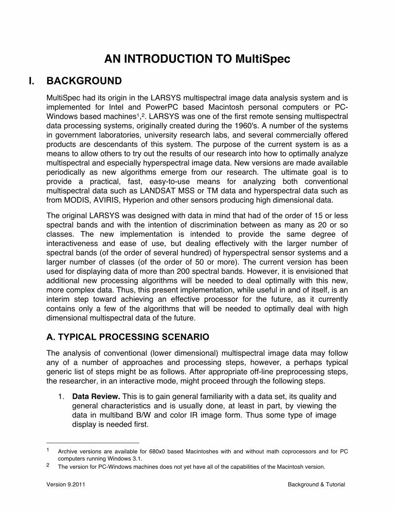
AN INTRODUCTION TO MultiSpec

I. BACKGROUND MultiSpec had its origin in the LARSYS multispectral image data analysis system and is implemented for Intel and PowerPC based Macintosh personal computers or PC-Windows based machines1,2. LARSYS was one of the first remote sensing multispectral data processing systems, originally created during the 1960's. A number of the systems in government laboratories, university research labs, and several commercially offered products are descendants of this system. The purpose of the current system is as a means to allow others to try out the results of our research into how to optimally analyze multispectral and especially hyperspectral image data. New versions are made available periodically as new algorithms emerge from our research. The ultimate goal is to provide a practical, fast, easy-to-use means for analyzing both conventional multispectral data such as LANDSAT MSS or TM data and hyperspectral data such as from MODIS, AVIRIS, Hyperion and other sensors producing high dimensional data. The original LARSYS was designed with data in mind that had of the order of 15 or less spectral bands and with the intention of discrimination between as many as 20 or so classes. The new implementation is intended to provide the same degree of interactiveness and ease of use, but dealing effectively with the larger number of spectral bands (of the order of several hundred) of hyperspectral sensor systems and a larger number of classes (of the order of 50 or more). The current version has been used for displaying data of more than 200 spectral bands. However, it is envisioned that additional new processing algorithms will be needed to deal optimally with this new, more complex data. Thus, this present implementation, while useful in and of itself, is an interim step toward achieving an effective processor for the future, as it currently contains only a few of the algorithms that will be needed to optimally deal with high dimensional multispectral data of the future. A. TYPICAL PROCESSING SCENARIO The analysis of conventional (lower dimensional) multispectral image data may follow any of a number of approaches and processing steps, however, a perhaps typical generic list of steps might be as follows. After appropriate off-line preprocessing steps, the researcher, in an interactive mode, might proceed through the following steps.

1. Data Review. This is to gain general familiarity with a data set, its quality and general characteristics and is usually done, at least in part, by viewing the data in multiband B/W and color IR image form. Thus some type of image display is needed first.

1 Archive versions are available for 680x0 based Macintoshes with and without math coprocessors and for PC

computers running Windows 3.1. 2 The version for PC-Windows machines does not yet have all of the capabilities of the Macintosh version.


Version 9.2011 - 2 - Background & Tutorial

2. Class Definition. Definition of the class of material to be identified or the set of classes to be discriminated between must be carried out. Some means for quantitatively defining the specific class characteristics of interest is required here. Often this is accomplished by the researcher labeling a small sample of the pixels from the data itself, as representative of the classes of interest. The analysis process then becomes an extrapolation from these samples, called training samples or design samples, to the entire data set.

3. Feature Determination. The specific features to be used in the analysis

must be identified or calculated. This may be simply a process of selecting an optimal subset of the available spectral bands, or there may be some calculation process to combine bands in some useful way.

4. Analysis. The specific analysis algorithm is applied to the data set to carry out the desired identification or discrimination.

5. Results Evaluation. Both quantitative and qualitative means are used to

determine the quality and characteristics of the results obtained.

The current implementation of MultiSpec provides some means for accomplishing each of these steps. The primary point of departure is that the analysis desired is one that is relative in nature, meaning that rather than identifying a single class of material in a subject vs. background mode, each pixel is to be assigned to a class based upon a judgment criterion relative to all possible classes. This implies that enough classes must be defined so that there is a logical class to which to assign every pixel in the scene, with the possible exception of a small number of pixels that will be determined by a threshold. Further, the current implementation assumes that the classes are made up of sums of multivariate Gaussian distributions. Tools such as histogramming and clustering are provided to assist in determining the modes of the data and to properly define classes and subclasses that reasonably fit this assumption. Finally, the current implementation is to be regarded as by no means complete. A number of new algorithms are under evaluation or development to broaden the circumstances under which the system will be effective and to make the process for user-efficient and convenient. B. THE MULTISPEC IMPLEMENTATION For this section, it is assumed that the reader is familiar with the standard user interface, and knows how to use pull-down menus, point, click, and drag with the mouse, etc. If this is not the case, the user should refer to the computer operating system manual or tutorials. The MultiSpec application should also be copied onto the hard disk, if it is not already there, as well as the data to be used. At this point,



• Start the MultiSpec application by double-clicking on it. Macintosh Version Upon opening the MultiSpec application, a Menu Bar and Text Output Window will be displayed as shown in Figure 1a. The Text Output Window is the window in which all text output from the program, such as file statistics, histogram data, and initial classification results will appear. Text data appearing there may be copied and pasted into other applications. Notice the list of menus across the top of the screen and in Figure 1a. By pointing with the cursor to each and holding the mouse button down, the various options of each menu item may be observed. In doing so, it is seen that the File menu allows one to open an Image or Project Image window for displaying that image in a window, to Print output, or to Save the text output to a disk file, among other things.

Figure 1a. The MultiSpec Menu Bar and Text Window. This is what appears on the screen upon start-up of MultiSpec on a Macintosh machine.

The Edit menu is used for standard user interface functions such as cutting, copying, pasting, and clearing or to change the Image Description or Image Map Parameters. The Project menu is used to control Project file settings. The Project file is the file used to store training and test field coordinates, class statistics, etc., so that one may save one's intermediate results and quit before completing an analysis. One can then restart the analysis at a later time without losing any work. The Processor menu allows one to choose the MultiSpec processor one wishes to use. The Options menu is needed only for advanced purposes and is explained in the Reference section. The Window menu is used to bring any given window to the front and make it the active window. One can also open selection graphs with this menu.



Windows Version Upon opening the MultiSpec application, an application window with a Menu Bar and Text Output Window will be displayed as shown in Figure 1b. The Text Output Window is the window in which all text output from the program, such as file statistics, histogram data, and initial classification results will appear. Text data appearing there may be copied and pasted into other applications. Notice the list of menus across the top of the application window and in Figure 1b. By pointing with the cursor to each and holding the mouse button down, the various options of each menu item may be observed. In doing so, it is seen that the File menu allows one to open an Image or Project Image window for displaying that image in a window, to Print output, or to Save the text output to a disk file, among other things.

Figure 1b. The MultiSpec Application Window, Menu Bar and Text Window. This is what appears on the screen upon start-up of MultiSpec on a Windows machine.

The Edit menu is used for standard user interface functions such as cutting, copying, pasting, and clearing or to change the Image Description or Image Map Parameters. The View menu controls the visibility of items like the Toolbar. The Project menu is used to control Project file settings. The Project file is the file used to store training and test field coordinates, class statistics, etc., so that one may save one's intermediate results and quit before completing an analysis. One can then restart the analysis at a later time without losing any work. The Processor menu allows one to choose the MultiSpec processor one wishes to use. The Options menu is needed only for advanced purposes and is explained in the Reference section. The Window menu is used to bring any given window to the front and make it the active window. One can also open selection graphs with this menu. The Help menu provides the About



MultiSpec window. The Toolbar allows short cuts to such actions as opening image windows and zooming image windows.

II. A TUTORIAL EXAMPLE A typical analysis task usually involves many classes, however, as a simple example, we will use a small portion of a Thematic Mapper data set to carry out a 2-class, 7 band classification. The two classes will be Green Vegetation and Other. The data is shown in Figure 2. We will use the three fields indicated in the figure as training data. The figures are from the Macintosh version but the screens from the Windows version will be very similar.

A. Display and Inspection of the Data To begin the example, open MultiSpec if it is not already and,

• From the File menu choose Open Image. . .. A dialog box will open to allow one to select the data file one wishes to use.

• Select TipJul1.tif and Open, or simply double-click on TipJul1.tif

Figure 2. An image presentation of the data in the file TipJul1.lan showing

fields to be used for training in part B.

1

Training Field for Veg

2

Training Fields for Other



This is a small segment (169 lines x 169 columns of pixels) of a Thematic Mapper scene of Tippecanoe County, Indiana gathered on July 17, 1986. Next a dialog box will appear to allow one to choose among various options for the image display.

• Note that by default the area designated for display is the whole scene and the 3-Channel Color Display Type is selected. The default settings call for the Red screen color to be derived from band 4 and the Green screen color from band 3 and the Blue screen colors from band 2. Any bands could be chosen, however, since band 4 is from the reflective infrared region and bands 3 and 2 from the visible red and green regions respectively, these particular choices are satisfactory for our use and will cause the screen image to be in a 3-color format approximating Color Infrared film. Therefore, click OK.

If the data histogram has not previously been calculated and stored, another dialog box will next be presented allowing the choice of regions to be histogrammed, so that the various channel gray values can be properly assigned to screen colors. The default options built into this dialog box are satisfactory, so

• Click OK to begin the histogramming.

After the histograms of the seven channels have been compiled, a dialog box will be presented allowing them to be stored so that they will not have to be re-compiled when this data set is next used. The default file title is satisfactory, so,

• Click Save to store the histogram in the image statistics file, TipJul1.sta.

Macintosh Version

The image of the data will next appear. First, use the window sizing box in the lower right corner of the image window to

• Enlarge the window to a little more than twice its current size by dragging it to the right and down.

Notice that just above the window sizing box, there are two small buttons for changing the scale of the image with icons representing a larger mountain (zoom in) and smaller mountain (zoom out). Just to the left of the window sizing box

is another box which shows ʻX 1.0ʼ in grayed form. This indicates the current zoom magnification.

• Click the larger mountain button once to magnify the image by a factor of 2.

1

Window Sizing Box

2

Image zoom buttons

Window Zoom Button



One can magnify further if one wants just by clicking additional times on the zoom in button. Reduce the magnification by clicking on the zoom out button. Any time the magnification is different from 1.0, one may click on the magnification size box to return it to x 1.0. After experimenting a bit, return the magnification to X 2.0. By clicking on the Window Zoom Button (right-most button in upper left corner of the window), one can adjust the window to just the size of the image. Windows Version

The image of the data will next appear. First, use the window sizing box in the lower right corner of the image window to

• Enlarge the window to a little more than twice its current size by dragging it to the right and down.

Notice that in the toolbar above the window, there are two small buttons for changing the scale of the image with icons representing a larger mountain (zoom in) and smaller mountain (zoom out). Just to the left of the

zoom icons is another box which shows ʻX 1.ʼ in grayed form. This indicates the current zoom magnification. One can magnify further if one wants just by clicking additional times on the zoom in button. Reduce the magnification by clicking on the zoom out button. Any time the magnification is different from 1.0, one may click on the magnification size button to return it to x1. After experimenting a bit, return the magnification to X 2.0. By clicking on the Window Zoom Button, one can adjust the window to take up all of the application window.

B. Training Sample Selection The next step is to select training fields. To do so,

• From the Processor menu select Statistics and click OK in the resulting

dialog box as we will use all seven spectral bands in statistics calculation and classification, and the other default values are satisfactory.

A new window labeled Project will appear in the upper right corner of the screen that will be used in a moment. To select training fields for each class, one must simply "drag" a rectangular area on the image (or, with polygon option selected, click on the corners of the desired polygon), and then "Add that field to the list." Thus,

Image zoom buttons

Window Zoom Button

Window Sizing Box



• Drag from the upper left corner to the lower right corner of the Veg. training

field in the image window (the upper one of Figure 2 that shows red on the screen). If upon inspection, one does not like the exact boundaries resulting, one may immediately repeat the process.

• Note in the Project window (Select Field View), that the coordinates (row and

column numbers) of the upper left corner and the lower right corner of the selected area appear there. Now,

• Click on the Add to list button.

A dialog box will appear to allow one to name the class and give the field a special designation, as desired. Thus,

• Type Veg into the Class Name box and then click OK. Since there is to be only one training field for this class, we are ready to select the training for the second training class. Thus next,

• Drag across the second training field in the Image Window shown in Figure

2. • Click on the Add to list button in the Select Field window.

Again, a dialog box will appear to allow one to name the class and give the field a special designation, as desired.

• Type Other into the Class Name box and then click OK. The class Other is to have two fields in its training set. Thus next,

• Point to the ʻNewʼ class name of the Select Field window and hold the Mouse button down. A pop-up menu will appear. Without releasing the mouse button, drag to Other and then let up on the Mouse button. Next,

• Drag across the remaining training field in the Image Window Since the class indicated in the Select Field window was set to Other, this field will automatically be associated with that class.

• Click on the Add to list button in the Select Field and click OK on the "Field 3"

dialog box that results. Since there are to be only two classes and a total of three training fields, the training process is complete, and we are now ready to evaluate the adequacy of our class



definition and training. In more typical circumstances, it would probably be desirable to check its quality in other ways, however, for now we will evaluate it only by classifying the training fields to see that they are appropriately separable.

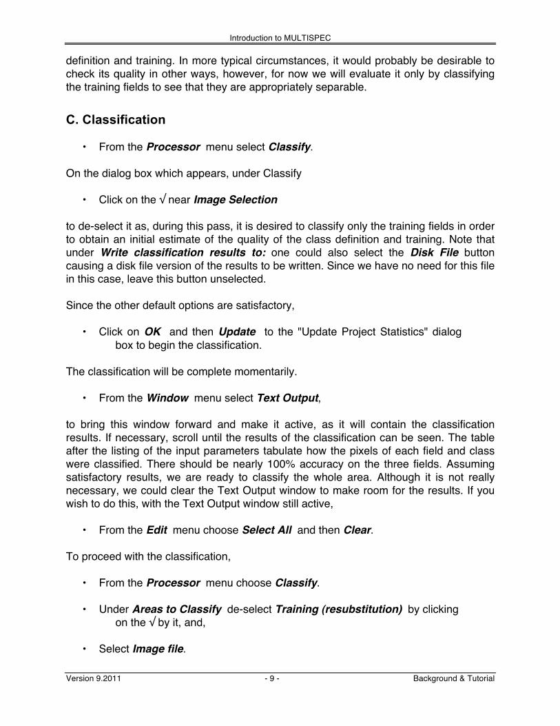
C. Classification • From the Processor menu select Classify.

On the dialog box which appears, under Classify

• Click on the √ near Image Selection

to de-select it as, during this pass, it is desired to classify only the training fields in order to obtain an initial estimate of the quality of the class definition and training. Note that under Write classification results to: one could also select the Disk File button causing a disk file version of the results to be written. Since we have no need for this file in this case, leave this button unselected. Since the other default options are satisfactory,

• Click on OK and then Update to the "Update Project Statistics" dialog box to begin the classification.

The classification will be complete momentarily.

• From the Window menu select Text Output,

to bring this window forward and make it active, as it will contain the classification results. If necessary, scroll until the results of the classification can be seen. The table after the listing of the input parameters tabulate how the pixels of each field and class were classified. There should be nearly 100% accuracy on the three fields. Assuming satisfactory results, we are ready to classify the whole area. Although it is not really necessary, we could clear the Text Output window to make room for the results. If you wish to do this, with the Text Output window still active,

• From the Edit menu choose Select All and then Clear. To proceed with the classification,

• From the Processor menu choose Classify. • Under Areas to Classify de-select Training (resubstitution) by clicking

on the √ by it, and, • Select Image file.



• Also click on Disk File under Write classification results to: so that a disk file for later use will be created. Then click OK. Also click Save to the dialog box that follows regarding a file name for the results.

It should take less than a second to classify the 28,561 pixels in the data set using all 7 bands. As soon as the classification is complete, one will see results displayed in the text window and one may want to scroll over the classified area to examine the results. The following table lists the actual lines and columns used for the training fields selected for this example. Classes used: Weight 1: Veg 10.000 2: Other 10.000 Training Fields Used: (line interval = 1; column interval = 1) First Last First Last Field name Class Line Line Col. Col. 1: Field 1 1 29 52 60 73 2: Field 2 2 59 69 32 56 3: Field 3 2 78 83 33 55



D. Obtaining a Hard Copy Printout Hard copy in Thematic Map form. A hard copy output in Thematic Map form may be obtained by the following.

• In the File menu, choose Open Image,

• In the resulting dialog box, select the file TipJul1.GIS that was generated by the classifier, and click Open. Click OK on the resulting dialog box.

One may change from the default color used for each class to more appropriate ones by double-clicking in the legend on the color to be changed, then clicking on the color desired in the color wheel resulting. For example, one may change to green for the Vegetation class. Note that colors of contrasting brightness should be chosen for the two classes if the intent is to subsequently print out a black and white version of the display as is the case here. One may enlarge the resulting image as desired using the zoom in botton on the lower right. Then,

• In the File menu, choose Print Image…, and OK on the resulting dialog box. Figure 3 shows an example of the result in color form. Note also that one may copy the display to a word processor document by choosing 'Select All' or by dragging over the portion of the display desired, then choosing 'Copy,ʼ and then pasting the result into the word processor document.

Figure 3. A classification result in color thematic map form.



E. Quantitative Check of Accuracy To assist in the evaluation of the analysis results, the LIST RESULTS processor may be used. To do so, first,

• Make certain that the TipJul1.gis window is active; (if it is not, click on any part of it showing or select it in the Windows menu),

• From the Project menu, select Add Associated Image.

The outlines and names of the training fields will immediately be shown on the image. Next,

• From the Processor menu, select List results. . .. A dialog box providing several options will appear. These options are all described in the Reference Section. For now,

• select Field under the Summarize by (train/test only) group. • click OK.

This will cause the system to generate in the text window two tables of results for the accuracy of the training samples, similar to the following.

TRAINING FIELD PERFORMANCE (Resubstitution Method) Project Reference Number of Samples in Thematic Image Class Field Class Accuracy+ Number 0 1 2 Name Number (%) Samples background Veg Other Field 1 1 100.0 336 0 336 0 Field 2 2 100.0 275 0 0 275 Field 3 2 100.0 138 0 0 138 TOTAL 749 0 336 413 TRAINING CLASS PERFORMANCE (Resubstitution Method) Project Reference Number of Samples in Thematic Image Class Class Class Accuracy+ Number 0 1 2 Name Number (%) Samples background Veg Other Veg 1 100.0 336 0 336 0 Other 2 100.0 413 0 0 413 TOTAL 749 0 336 413 Reliability Accuracy (%) 100.0 100.0 OVERALL CLASS PERFORMANCE ( 749 / 749 ) = 100.0% Kappa Statistic (X100) = 100.0%. Kappa Variance = 0.000000. + (100 - percent omission error); also called producer's accuracy. * (100 - percent commission error); also called user's accuracy.



The first table provides an accuracy assessment for the training fields. Each line of the table contains the results for one of the training fields. The second table combines the fields of each class to show the overall training class results. If Test Fields had been defined, similar tables could be calculated for these as well. A capability to Group classes, i.e., combine classes that are actually subclasses of a more general class, is described in the Reference section of this document, under the Open Image command of the File menu. If such Grouping had been done, tables as above could be determined for Groups as well.

F. Clustering Algorithms Two Clustering Algorithms are contained in MultiSpec. They are useful in the classifier training step in determining how many classes might be separable in a given data set, and in finding the modes of data. One algorithm implemented is a simple one-pass type. The second is of the iterative type. More information on these algorithms is contained in the Using MultiSpec and Reference sections of this document.

G. The Feature Selection Processor

A Feature Selection Processor is included to assist in choosing a best subset of spectral features to be used for a specific classification. For example, instead of using all seven TM bands in the above tutorial example, it may have been better to choose the best three of the seven bands for the particular pair of classes. This would certainly have saved computation time, and in a more complex classification task, it may have provided higher classification accuracy. The Feature Selection Processor produces a table showing the statistical distance between each of the class pairs for each of the possible subsets of features. In a case of three classes, the best three of seven features and the Bhattacharyya statistical distance measure, the results that appear in the text window are as follows:

Feature Selection 04-16-2011 18:26:40 (MultiSpecUniversalPPC_12.15.2010) Input Parameters: Project = 'TIPJUL1_for_intro_3class.Project' Original class statistics are used. Base image file = 'TipJul1.tif' Algorithm used is "Bhattacharyya" List best 12 combinations. Minimum value to be listed: 0 Maximum value to be listed: 30000 List separability table. 1 contiguous channels in each channel combination group All possible channel combinations will be searched Channels used: 1: 0.45- 0.52 um 2: 0.52- 0.60 um



3: 0.63- 0.69 um 4: 0.76- 0.90 um 5: 1.55- 1.75 um 6: 2.08- 2.35 um 7: 10.4 -12.5 um Classes used: Symbol 1: Veg 1 2: Other 2 3: 2nd other 3 Output Information: There are 3 class combinations. There are 35 channel combination(s) for 3 group(s) of 1 contiguous channel(s). class pair symbols > 12 13 23 weighting factor > (10) (10) (10) Channels Min. Ave. Weighted Interclass Distance Measures 1. 2 6 7 1.06 9.48 11.3 16.0 1.06 2. 5 6 7 1.00 11.37 18.3 14.7 1.00 3. 3 6 7 0.99 9.07 8.57 17.6 0.99 4. 4 6 7 0.99 8.56 7.21 17.4 0.99 5. 1 6 7 0.97 8.59 7.05 17.7 0.97 6. 4 5 7 0.78 12.69 15.5 21.7 0.78 7. 1 2 7 0.73 7.85 11.3 11.4 0.73 8. 1 4 7 0.66 7.07 7.64 12.9 0.66 9. 2 5 7 0.66 9.53 10.9 16.9 0.66 10. 1 2 6 0.63 5.94 7.73 9.45 0.63 11. 1 3 7 0.63 6.60 7.94 11.2 0.63 12. 1 5 7 0.62 9.40 9.79 17.7 0.62

0 CPU seconds for feature selection. 04-16-2011 18:26:41 (Note that the coordinates for the field representing “2nd other” class are lines 30-37 and columns 100-110 if one wishes to try to replicate the listing.) By choosing the correct option, the subsets of channels have been listed in descending order according to the minimum of the Weighted Interclass Distance values. (Another option would have the subsets listed in descending order according to the average of the Weighted Interclass Distance values.) Note from the table, this algorithm suggests that Channels 2, 6, and 7, would be the best three for discriminating among these three classes. However, though the minimum interclass separability for n-tuple 2, 6, 7 is the largest, if one were more concerned about good separation between classes 1 and 3, channels 4, 5, and 7 might be a better choice, since it has a maximum interclass distance of 21.7. In general, in using this processor, one would want to scan both the Average column and the Minimum column of the processor output, perhaps in addition to reviewing the individual entries appearing in the table of Weighted Interclass Distance Measures. One could also use the Weights option to vary the interclass distance weighting in the averaging process to assist evaluation when there are a large number of classes. Alternatively, the Feature Selection Processor output may either be copied and pasted to a spreadsheet, or saved on disk as a text file and opened from a spreadsheet for



more complex study of the table. Other example uses of commercially available software are contained in the following section.

H. Example Use of Other Software. The use of commercial applications such as a graphing program can be very useful in extending the capabilities of MultiSpec, and indeed, such use is an intention of the design of it. As another example, Figure 4 shows a histogram of every fifth line and every fifth column of the data set for bands 3 and 4. This figure was obtained by choosing the Histogram Processor with the List Histogram option selected, and then copying the result from the Text Output window and pasting it into a commercially available graphing application program.

Figure 4. Histogram of TipJul1.tif in bands 3 and 4.

Note that since the above example was created, MultiSpec now has the capability to make histogram graphs. The point of the section is to illustrate how one can copy data from MultiSpec to other applications for additional analyses.

Digital Value

Num

ber

of

Pixe

ls

0

20

40

60

80

100

120

140

160

180

0 20 40 60 80 100

120

140

160

180

200

4

3

Using MULTISPEC

Version 9.2011 - 16 - Using MultiSpec: Importing Data

III. Using MultiSpec

A. Importing data MultiSpec is able to read most any data file in Binary or some data in ASCII format provided that the parameter values in the following dialog box are known.

ASCII format refers to images represented by alphanumeric characters - one character for each pixel. MultiSpec cannot interpret ASCII image files represented by numbers separated by commas or spaces. MultiSpec will attempt to determine these parameters from the header portion of the selected data file. See Appendix E for a list of the image file formats that MultiSpec recognizes. If MultiSpec is unable to determine the parameters for the file format, the above dialog box will be displayed to allow one to specify the parameters. Acceptable limits on several of these parameters are listed in Appendix B. Band interleave formats which are acceptable are Band Interleaved by Line (BIL), Band Sequential (BSQ), and Band Interleaved by Sample (BIS). The data may have either one, two or four bytes (8, 16 or 32 bits, respectively) per sample for integer data values and four or eight bytes (32 or 64 bits respectively) per sample for real data. In the case of two, four or eight bytes, the bytes may be in either least significant byte or most significant byte order.

Using MULTISPEC

Version 9.2011 - 17 - Using MultiSpec: Importing Data

The file to be imported may or may not have a header or trailer, but if it has either, the format of it does not need to be known, only the number of bytes included. The image data file may have additional bytes included before and/or after each line or channel; these bytes may be for storage of information such as line numbers or calibration data, but again only the number of bytes involved needs to be known. MultiSpec will ignore header, trailer, pre-line, post-line, pre-channel and post-channel bytes when displaying the data. An example format that uses several of these parameters is the LARSYS MIST format. These files are BIL with a header of 800 bytes and 4 pre-line calibration bytes and 6 post-channel calibration bytes. The pre-line bytes are at the beginning of each line of data and the post-channel bytes are at the end of each channel of data. In other words, there are a total of n channels times 6 bytes of post-channel bytes for each line of data. If this image file is actually a subset of a larger image file and it is desired to retain the line and column numbers from the original, the above dialog box provides a capability to enter those data at the time the data are first read by MultiSpec using the "start line" and "start column" parameters. Upon reading the file for the first time, each of these data values must be entered or chosen, after which, if desired, MultiSpec can re-write the data with a known header so that these items will not have to be re-entered when this file is next displayed. Then the steps needed to import new data are as follows. Store the data file in either binary or ASCII format in a data volume accessible to MultiSpec. Open MultiSpec and choose Open Image from the File menu. The usual dialog box will appear allowing you to choose the data volume and data file containing the new data. Upon clicking OK, the dialog box above will appear. Upon entering the correct parameter values and clicking OK, the image data will be read into MultiSpec, and the "Set Display Specifications" dialog box will appear (see Open Image under the File Menu in the Reference Section). The data have thus been successfully imported. If it is desired to have a standard header inserted to the file, so that the file parameters do not have to be re-entered the next time the file is opened, after the above steps, choose Reformat... from the Processor menu, then select Insert Header. A dialog box will be displayed to allow one to insert an ERDAS74 header. One can add a few additional header types, including TIFF/GeoTIFF or ArcView, by using the Reformat Processor “Change Image File Format” Command. (See Reference Section).

MULTISPEC REFERENCE

Version 9.2011 - 18 - Using MultiSpec: Analyzing Data

B. Analyzing Data Background and Procedure. There are many approaches to analyzing multispectral image data, almost as many as there are analysts. The steps used in any given analysis must necessarily be based upon the scene, the information desired, and the data analyst's initial assumptions about the data characteristics. The basic requirement of an analysis process is,

• To divide the entire multi-dimensional data space defined by the data set into

an exhaustive set of non-overlapping regions in such a way that the regions delineated, or an appropriate subset of them, correspond as precisely as possible to data points belonging to the particular classes desired.

Experience has shown that, properly used, the assumption that each of these data subsets may be modeled in terms of one or a combination of Gaussian distributions is a quite practical and powerful way to proceed. Among the advantages of using the Gaussian model is the mitigation of need for large training sets to properly define the desired classes, especially when the spectral dimensionality is large. However, use of this assumption does impose upon the analysis process, some means for identifying the various modes of each desired information class, and the fitting of densities to each of these modes. The analysis process then consists of finding the parameters for a collection of Gaussian distributions which fit the entire data set, and for which some subset of the distributions correspond to the classes of interest. With regard to dealing with confounding scene observation variables such as the atmosphere, illumination and view angles, terrain relief, etc., one approach is to attempt to pre-adjust the data before analysis to account for the variation introduced by each of these confounding variables into spectral responses. However, as a practical matter, the lack of adequately precise values for the parameters of such scene variables, the complexity of the calculations required even if the parameter values are known, and the noise and uncertainties introduced by such calculations (which themselves can tend to reduce the amount of information that could ultimately be obtained from the data) are disadvantages of this approach. A second approach is to use analysis techniques that are relatively insensitive to such scene observation variables in the first place. The various conditions in which a desired information class exists in the data may be handled by defining additional subclasses for the desired information classes. This is the approach in mind in the following, and a minimum amount of pre-analysis adjustment to the data is assumed to have been used.

MULTISPEC REFERENCE


The steps below, then, allow for accomplishing the analysis task according to the above approach using MultiSpec3. 1. Familiarization with the data set.

• Display the data in two or three color format using the Display Image processor to assess its general qualities4. Compare the displayed image with any ground reference information about the site that may be available. Compose a tentative list of classes which is adequately (but not excessively) exhaustive for this data set.

2. Preliminary selection of the classes and their training sets.

• Using the Cluster processor, cluster the area from which training fields are to be selected, saving the results to disk file. Display the resulting thematic map for use in marking training areas.

• Using either the display of the original data or that of the thematic cluster map

(after adding it as an associated image), make a preliminary selection of training fields which adequately represent the selected classes.

3. Verification of the class selection and training.

• Use the Feature Selection processor to determine the degree of separability between the various classes. Check the modality of the classes by examining the cluster map or by clustering the training areas. Where multi-mode classes are found, it may be appropriate to define two or more sub-classes to accurately represent the entire class. It may be desirable to iterate between steps 2 and 3.

• It may also be useful to examine the histograms of each class using the

Statistics Processor to determine the need for subclasses. This is another means of identifying the need for subclasses.

4. Selection of the spectral features to be used.

• Once a reasonably final training set is arrived at, use the Feature Selection processor to choose the best subset of features for carrying out the classification for a given training set5.

3 The procedure described here is relative to a data set of conventional dimensionality (<20 bands). For

hyperspectral data sets with 50 to 500 bands, an augmented procedure would be needed and is described in other documents on https://engineering.purdue.edu/~biehl/MultiSpec/documentation.html.

4 It may also be useful to display the data in side-by-side format to see that all bands of data are present and of reasonable quality at least in terms of subjective appearance.

5 The Feature Extraction processor is also available for this task. See the discussion on this processor later in this section.

MULTISPEC REFERENCE


5. Preliminary Classification of the data.

• Classify the training fields only, using the spectral bands you have selected to verify their purity and separability.

6. Final Classification, Evaluation of the classification and Extraction of the desired information.

• Classify the entire data set using the features selected.

• Mark as many fields as possible as Test Fields using the Statistics Processor.

Use the List Results processor to determine the accuracy obtained on the training fields and to determine how well the classifier training generalizes beyond the training set. Make modifications to the training as required to obtain satisfactory results at this point.6

• Depending upon the results of these evaluations it may be necessary to repeat

previous steps after modifying the class definitions and training. After becoming satisfied with the results, classify the entire data set, perhaps setting a modest threshold value, saving the classification results to a disk file, and creating a Probability Results file.

• Use the Display Image processor to generate thematic map versions of the

results and the Probability Results files for subjective evaluation purposes. The classification results file display is useful in determining that the classification results are appropriate and consistent from a spatial distribution standpoint. The portion of points thresholded in the results display, together with the Probability Results file helps to determine if any important modes in the data have been missed in the class definition process. Depending on the outcome, it may again be necessary to iterate using some of the above steps. The List Results processor can be used to provide a quantitative evaluation of the results based upon the accuracy figures of the training and test fields classification.

Some Example Uses of System Capabilities. In the following we shall sample several of the above steps to demonstrate how MultiSpec may be used. We note that all of the features of MultiSpec are cataloged in the Reference Section of this document. Our purpose here is more to illustrate how some of the varied capabilities of MultiSpec can be used in the process of analyzing a data set rather than to delineate a practical procedure for a given problem. 6 The Enhance Statistics processor may be used to improve the extent to which the classifier successfully

generalizes from the training to the other samples of the data set. See the discussion on this new processor later in this section.

MULTISPEC REFERENCE


For this purpose, we will again use TipJul1.tif, the same data set as in Section II (Tutorial) above. Begin by Opening MultiSpec, and displaying the ground reference file JTIPSUB1.gis, using Open Image from the File menu. Also display the file TipJul1.tif containing the multispectral data. We will assume that our primary interest in this analysis is on the classes Corn, Soybeans, and Alfalfa/Oats. With the TipJul1.tif image window active (the top window), choose Cluster... from the Processor menu. Choose the ISODATA algorithm, and on the resulting dialog box, choose the Use single-pass clusters initialization option for this example. The default choices under Other Options (convergence 99%; minimum cluster size = 8; distance1 = 25.1; distance2 = 50.2) will cause 11 clusters to be identified. Click OK on this dialog box, and set the Image Area choice under Cluster Classification Map Area(s) and the Text Disk File option under Write Cluster Map/Results to. Click OK to begin the processing and click Save to save the results to disk, using TipJul1_using.cluster as the name of the output file. (The name is modified so that the base name is not the same as that for the files generated in the Tutorial section above.) After the clustering is complete, Open the TipJul1_using.cluster image, and carefully compare it with the ground reference map, JTIPSUB1.GIS. As can be seen, some of the fields do belong uniquely to some of the desired information classes, some fields are made up of mixtures of two or more clusters, and some clusters appear to belong to two or more information classes, indicating that spectral classes must be defined in such a way as to split these clusters in the final classification. The task that remains then is to define spectral classes which match the desired information classes, and the cluster map can be a useful tool in this process. For example, note that Cluster 6 corresponds to some of the Soybean fields, and may, therefore, be suitable as one subclass of the information class Soybeans. Similarly for Cluster 11 and Corn. It will facilitate such a comparison to adjust the colors used for displaying Soybeans and Corn in the cluster map to those used on the ground reference image.

A way to do this with the Macintosh version is to double-click on the Cluster 6 color chip in the legend to obtain a color palette window, select the magnifying glass icon, and use it to select the color for soybeans in the ground reference image and click OK in the color palette window.

For with Windows version, double-click on the Cluster 6 color chip to obtain the color palette window and enter 125, 255 and 0 for red, green and blue, respectively. This will cause the color for Cluster 6 to be the same as for soybeans in the ground reference image.

You may wish to repeat these steps to change the color used for Cluster 11 to that of the Corn class as well. (The color for corn is: 248, 165 & 0 for red, green & blue.)

MULTISPEC REFERENCE


You may have noticed that a Project window appeared after running the Cluster processor. The cluster statistics were automatically saved to a project in memory. This is illustrated by the list of the 11 cluster classes in the Project window. The cluster class statistics could be used, for example, with the Feature Selection processor to determine the statistical distance between the various clusters, and this can be helpful in deciding if there are clusters which may be grouped together to form an information class of interest. To illustrate this, choose Feature Selection from the Processor menu, set the Channel Combinations option to a subset of 7 and using the Symbols pop-up box, set the symbol for cluster 6 to S (for soybeans) and cluster 11 to C (corn), and click on the List Options button. In the resulting dialog window, click on the List class pair distances option, then click OK, and click OK on the remaining window. When the calculation is complete, make the Text Window active and copy the lines listing the class pair symbols and their interclass distances. Open a spreadsheet application7 and paste the clipboard data in place. The class pairs may be sorted to find those separated by the smallest distances by the following. Select the columns containing the class pair distances (Columns E through BG in this case), choose Sort from the Data menu. Use the Options… button if needed to sort left to right. Sort by Row 4 and Smallest to Largest. Click OK and the left portion of the resulting table should look like the following.

The distance between 7 and 8 is the smallest and is seen to be 1.10, which indicates that clusters 7 and 8 are very near to one another, and perhaps may be grouped together. Adjust the color of cluster 8 to be the same as cluster 7 by the above technique and note the relationship of the two on the cluster map. A convenient means for assisting in this is as follows. With the cluster map window active and the shift key depressed, move the cursor onto the color of cluster 8 in the legend. Notice that the cursor turns into an eye. Now click the mouse button and notice that all of the pixels of the image in that cluster blink as you do so. (Holding down the control and the shift keys and clicking the mouse button causes all pixels in the other cluster classes to blink.) A careful comparison of the cluster map with the ground reference map will reveal that some of the pixels in the combined clusters 7 & 8 are soybeans and some are in other classes, thus although they are near to one another in 7-dimensional space, the classifier must split this combined cluster appropriately. We can arrange for this by using the cluster map to define training fields in two different classes. We will illustrate this process next. 7 We will indicate the commands to be used if Microsoft Excel is the spreadsheet being used, but any other

spreadsheet could be used as well.

MULTISPEC REFERENCE


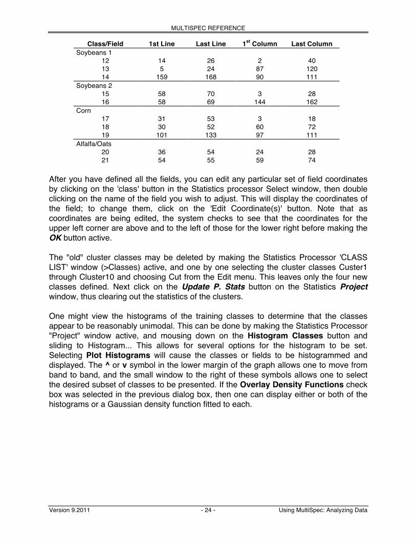
With the cluster map window active, select Add As Associated Image from the Project menu. This allows us to define training fields for the current project from this cluster map. On the image below, we show some training fields used to define "new" classes. For reference, the field coordinates are given in the table below the image. Define these fields as training areas in your project by designating them on the cluster map. When you define each class, have "New" showing in the Class pop-up window at the top of the Select Field window, so that you are defining new classes rather than adding to classes defined by the clustering. For defining the small fields, you may want to increase the magnification of the image. It is probably easiest to use the “Edit Selection…” button in the Project ʻSelect Fieldʼ Window.

Training Fields for Four Preliminary Classes.

(Note that for the image above the color of the lines used to outline the training areas was changed from white to black using the option in the Processor->Statistics dialog box.)

MULTISPEC REFERENCE


Class/Field 1st Line Last Line 1st Column Last Column Soybeans 1

12 14 26 2 40 13 5 24 87 120 14 159 168 90 111

Soybeans 2 15 58 70 3 28 16 58 69 144 162

Corn 17 31 53 3 18 18 30 52 60 72 19 101 133 97 111

Alfalfa/Oats 20 36 54 24 28 21 54 55 59 74

After you have defined all the fields, you can edit any particular set of field coordinates by clicking on the 'class' button in the Statistics processor Select window, then double clicking on the name of the field you wish to adjust. This will display the coordinates of the field; to change them, click on the 'Edit Coordinate(s)' button. Note that as coordinates are being edited, the system checks to see that the coordinates for the upper left corner are above and to the left of those for the lower right before making the OK button active. The "old" cluster classes may be deleted by making the Statistics Processor 'CLASS LIST' window (>Classes) active, and one by one selecting the cluster classes Custer1 through Cluster10 and choosing Cut from the Edit menu. This leaves only the four new classes defined. Next click on the Update P. Stats button on the Statistics Project window, thus clearing out the statistics of the clusters. One might view the histograms of the training classes to determine that the classes appear to be reasonably unimodal. This can be done by making the Statistics Processor "Project" window active, and mousing down on the Histogram Classes button and sliding to Histogram... This allows for several options for the histogram to be set. Selecting Plot Histograms will cause the classes or fields to be histogrammed and displayed. The ^ or v symbol in the lower margin of the graph allows one to move from band to band, and the small window to the right of these symbols allows one to select the desired subset of classes to be presented. If the Overlay Density Functions check box was selected in the previous dialog box, then one can display either or both of the histograms or a Gaussian density function fitted to each.

MULTISPEC REFERENCE


The following histogram plot for channel 4 shows the bimodal nature of the soybeans class discovered by the clustering process.

Assuming reasonable modality of the training classes, one may next carry out a trial classification. Assume one decides to use the best four of the seven bands for the classification. Choose Feature Selection from the Processor menu, and set the Channel Combinations option to a subset of size 4. If desired, you may set the Symbols to a user defined set, e.g.: S-Soybeans1, s-Soybeans2, C-Corn, and A-Alfalfa/Oats (note that this option is not available in the Wiindows version). Also set the Soybeans1 and Soybeans2 (Ss) class pair weight to 0 using the Weights option. Choose List Options..., and choose the Average class distance for the Sort combinations by option and check the List class pair distances check box. Click OK on both dialog windows. The results displayed in the Text window indicate that bands 2, 3, 4, and 5 would be the best to use. Choose Classify from the Processor menu, set Channels to a subset of 2, 3, 4 & 5 (first select "none", then click on 2 and with the shift key down, click on 3, 4, and 5), set Area to be Classified to the entire image area, and set the Write Classification Results To Disk File and Create Probability Results File and leave the Threshold check box unchecked. Then click OK. Set the base output file name (i.e. name before .gis) to be “TipJul1_4class”. When the classification is complete Choose Open Image from the File menu and select the classification file that was just created (name will be TipJul1_4class.gis). Then select OK in the resulting “Set Thematic Display Dialog” box to display an image of the classification. Now mouse down on the Classes pop-up menu of the legend and choose Groups/Classes. In the legend area, drag the Soybeans 2 class name up to the Soybeans 1 class name. Double-click the Soybeans 1 Group name and change it to just

MULTISPEC REFERENCE


Soybeans. Change the colors used for the classes to conform to those of the ground reference file JTIPSUB1.GIS. The resulting image is shown below, with the ground reference image for comparison. Note that we did not train for some of the minor classes and we did not use a threshold, so that all pixels where forced into one of the four classes (or three information groups) we set up.

The List Results Processor is useful in quantitatively estimating the accuracy of a classification. For example, in the case of this classification, one can check the accuracy of classification of the training samples by choosing List Results... from the Processor menu. The results may be obtained for fields, classes, and groups, based upon the options selected in the resulting dialog box. The results for the groups in this case are as follows.

TRAINING GROUP PERFORMANCE Project Number of Samples in Thematic Image Group Group Group Percent Number 1 2 3 Name Number Correct Samples Soybeans Corn Alfalfa/Oats Soybean 2 99.8 1973 1969 1 3 Corn 3 99.6 1162 1 1157 4 Alfalfa/Oats 4 100.0 127 0 0 127 TOTAL 3262 1970 1158 134

OVERALL PERFORMANCE (3253 / 3262 ) = 99.7 Kappa Statistic (X100) = 99.5%. Kappa Variance = 0.000003.

MULTISPEC REFERENCE


Test fields, i.e. fields specified by either rectangular or polygonal coordinates but not used as training samples could also be defined using the Project “Select Field” Window and tabular result for these fields could also be obtained using the List Results Processor. In fact use of test field are a better method of estimating classification performance since they would represent an unbiased estimate. It appears that the results are already reasonably good, but some additional work is needed on the Alfalfa/Oats class and other classes. An additional tool to accomplish this is available by displaying the Probability Results File created during the Classification process. Display this file by selecting Open Image from the File menu and then select “TipJul1_4classProb.gis”. This image, shown below, shows the probability of class membership for the most likely class. Red colors indicate high likelihood, and blue low likelihood. Regions with low likelihood are candidates for the definition of additional spectral classes. One notices upon inspection of this image that some of the clusters which we ignored above, need to be used to define additional spectral classes.

Probability Results Image

Note also from this Probability Results image that, in general, only the training areas tend to be the ones with the highest likelihood values. This indicates that the classifier does not generalize to non-training data of the same class as well as it might. This can be made clear by choosing Add as Associated Image from the Project menu while the Probability Results image is active. The training areas are then displayed on the Probability Results image, making the comparison easy.

MULTISPEC REFERENCE


One of the fundamental goals in analysis of such data is that the list of classes must be exhaustive, i.e., there must be a logical class to which to assign every pixel in the scene. The dark areas of the Probability Results image shows that this goal has not yet been met. Thus we shall select the following additional fields as classes, and let us treat the classes as unknowns at this point.

Class 1st Line Last Line 1st Column Last Column Unknown1 64 70 31 57 Unknown2 29 55 100 112 Unknown3 72 83 59 79 Unknown4 29 40 142 147 Unknown5 79 84 32 55 Unknown6 103 112 32 54 Unknown7 130 141 7 25 Unknown8 2 27 142 151

Add these fields as classes to the project file using the Project “Select Field” Window as before. Upon carrying out the 12-class classification and displaying the results, by adjusting the colors of the display to correspond with the ground reference map, it can be seen that all of the unknowns are soybeans except Unknown4 which is transportation. Though still some further refinement of the class definitions would be possible, the classification now fairly closely resembles the ground reference map. See the classification map shown below. However, there is one more modification we can make to the training statistics, improving another aspect of the training. Enhance Statistics. Another tool in MultiSpec is a processor called Enhance Statistics.8,9,10,11,12. Fundamental signal processing theory dictates that, for a classifier to be well trained,

• The list of classes must be exhaustive, in the sense that there is a logical class to which to assign every pixel in the scene,

• The classes must be separable using the available features, and

8 Behzad M. Shahshahani and David A. Landgrebe, "Using Partially Labeled Data For Normal Mixture

Identification With Application To Class Definition," Proceedings of the International Geoscience and Remote Sensing Symposium (IGARSS'92), Houston, TX, pp. 1603-5 May 26-29, 1992.

9 B.M. Shahshahani, D.A. Landgrebe, "On the Asymptotic Improvement of Supervised Learning by Utilizing Additional Unlabeled Samples; Normal Mixture Density Case," SPIE Int. Conf. Neural and Stochastic Methods in Image and Signal Processing, San Diego, CA, July 19-24, 1992.

10 Behzad M. Shahshahani and David A. Landgrebe, “Use Of Unlabeled Samples For Mitigating The Hughes Phenomenon” Proceedings of the International Geoscience and Remote Sensing Symposium (IGARSS'93), Tokyo, pp. 1535-7, August 1993.

11 Behzad M. Shahshahani and David A. Landgrebe, “Classification of Multi-Spectral Data By Joint Supervised-Unsupervised Learning,” PhD thesis, School of Electrical Engineering, Purdue University, December 1993, School of Electrical Engineering Technical Report TR-EE-94-1, January, 1994.

12 Behzad M. Shahshahani and David A. Landgrebe, “The Effect of Unlabeled Samples in Reducing the Small Sample Size Problem and Mitigating the Hughes Phenomenon,” IEEE Transactions on Geoscience and Remote Sensing, Vol. 32, No. 5, pp 1087-1095, September 1994.

MULTISPEC REFERENCE


• The classes must be of informational value, i.e. they must be classes of interest to the user.

An equivalent statement to this is that a well-trained classifier must have successfully modeled the distribution of the entire data set, but it must be done in such a way that the different classes of interest to the user are as distinct from one another as possible. What is desired in mathematical terms is to have the probability density function of the entire data set modeled as a mixture of class densities, i.e.,

p(x|θ) = ∑i=1

m αipi(x|φi) (1)

where x is the measured feature (vector) value, p is the probability density function describing the entire data set to be analyzed, pi is the density function of class i desired by the user, αi is the weighting coefficient or probability of class i, and m is the number of classes. The parameters θ and φi are to be discussed next in the context of what limitations are appropriate to the form of these densities. As is well known, the Gaussian assumption for class distributions is very convenient, as the Gaussian density function has many convenient properties and characteristics, both theoretically and practically. However, one cannot always assume that classes will be Gaussianly distributed, and a more flexible and general model is needed. On the other hand, a purely nonparametric approach is frequently not tractable in the remote sensing situation, as very large training sets are usually required to provide precise enough estimates of nonparametric class densities, while,

• It is a characteristic of the remote sensing application of pattern recognition theory that there will be a paucity of training samples.

As it turns out, a very practical approach is to model each class density by a linear combination of Gaussian densities. Thus, rather than having a single component of equation (1) represent a user class, the number of components in the combination can be increased, with different subsets of them representing each class. In this way, a very general capability can be provided, while still maintaining the convenient properties of the Gaussian assumption. Indeed, theoretically, every smooth density function can be approximated to within any accuracy by such a mixture of Gaussian densities. Thus for a well trained classifier, p(x|θ), the probability density function of the entire data set, can be modeled by a combination of m Gaussian densities. Assume that there are J (user) classes in the feature space denoted by S1...,SJ, J ≤ m. Each class consists of a different subset of the m Gaussian components, and indicate that component i belongs to class Sj by i ∈ Sj. Thus in equation (1), φi = (µi, Σi), the mean vector and covariance matrix, respectively, of Gaussian component i, and θ = (α1, ... , αm, µ1, ... , µm, Σ1 ... , Σm). All of the conditions required above are met if θ can be determined so that equation (1) is satisfied in such a way that the J classes are adequately separable and

MULTISPEC REFERENCE


correspond to user classes. Determining these m components is what must be accomplished by the training phase. How is this accomplished with MultiSpec? Returning to the three fundamentals stated above,

• The last of the three requirements, i.e., classes must be of informational value, is serviced by the user defining the training samples accordingly.

• The second one, classes must be separable, is supported by the use of a clustering algorithm in conjunction with the training process.

• The first of the three is assisted by the use of the MultiSpecʼs Probability Results map of preliminary classifications, since this allows one to locate pixels in the data set that, while having been assigned to a class, the strength of the class association is very limited, as evidenced by the likelihood of the most likely class being very low.

However, to this point, none of these tools tends to guarantee that equation (1) is indeed satisfied, i.e., the combination of class conditional density functions defined in this process provide a good model of the entire data set to be analyzed. It is this problem that the Enhance Statistics processor is designed to solve. The Enhanced Statistics process uses the training samples together with a uniformly selected set of (unlabeled) samples from the entire data set in an iterative fashion to adjust the class means and covariances so that the combination of class densities better fit the entire density. From the application point of view, this process has several possible benefits.

(1) The process tends to make the training set more robust, providing an improved fit to the entire data set, thus providing improved generalization to data other than the training samples.

(2) The process tends to mitigate the Hughes phenomena, i.e., the effect that, for a

finite sized training set, as one adds more features, the accuracy increases for a while, then peaks and begins to decrease. This problem of declining accuracy for increasing numbers of features is especially of concern when either a) the training set size is small, or b) the number of features available is large or both. Enhancing the statistics by this scheme tends to move the peak accuracy vs. number of features to a higher value at a higher dimensionality, thus allowing one to obtain greater accuracy with a limited training set.

(3) An estimate is obtained for the prior probabilities of the classes, as a result of the

use of the unlabeled samples, something that cannot be done with the training samples alone.

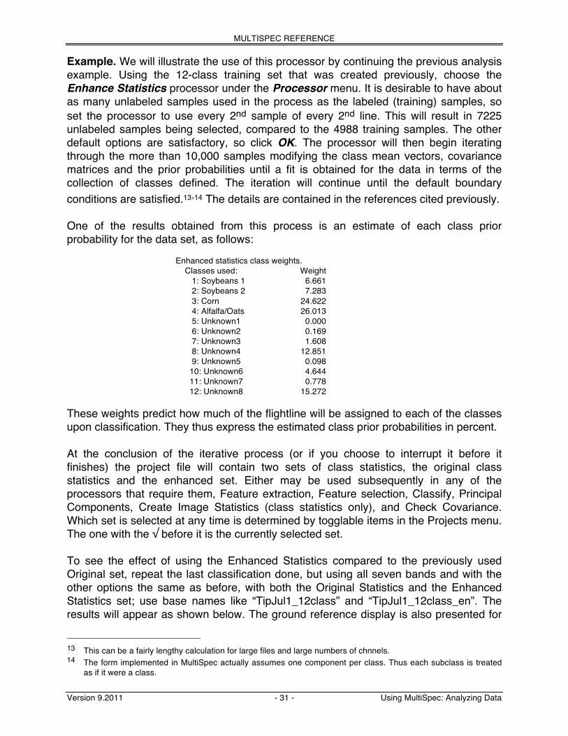
MULTISPEC REFERENCE


Example. We will illustrate the use of this processor by continuing the previous analysis example. Using the 12-class training set that was created previously, choose the Enhance Statistics processor under the Processor menu. It is desirable to have about as many unlabeled samples used in the process as the labeled (training) samples, so set the processor to use every 2nd sample of every 2nd line. This will result in 7225 unlabeled samples being selected, compared to the 4988 training samples. The other default options are satisfactory, so click OK. The processor will then begin iterating through the more than 10,000 samples modifying the class mean vectors, covariance matrices and the prior probabilities until a fit is obtained for the data in terms of the collection of classes defined. The iteration will continue until the default boundary conditions are satisfied.13,14 The details are contained in the references cited previously. One of the results obtained from this process is an estimate of each class prior probability for the data set, as follows:

Enhanced statistics class weights. Classes used: Weight 1: Soybeans 1 6.661 2: Soybeans 2 7.283 3: Corn 24.622 4: Alfalfa/Oats 26.013 5: Unknown1 0.000 6: Unknown2 0.169 7: Unknown3 1.608 8: Unknown4 12.851 9: Unknown5 0.098 10: Unknown6 4.644 11: Unknown7 0.778 12: Unknown8 15.272

These weights predict how much of the flightline will be assigned to each of the classes upon classification. They thus express the estimated class prior probabilities in percent. At the conclusion of the iterative process (or if you choose to interrupt it before it finishes) the project file will contain two sets of class statistics, the original class statistics and the enhanced set. Either may be used subsequently in any of the processors that require them, Feature extraction, Feature selection, Classify, Principal Components, Create Image Statistics (class statistics only), and Check Covariance. Which set is selected at any time is determined by togglable items in the Projects menu. The one with the √ before it is the currently selected set. To see the effect of using the Enhanced Statistics compared to the previously used Original set, repeat the last classification done, but using all seven bands and with the other options the same as before, with both the Original Statistics and the Enhanced Statistics set; use base names like “TipJul1_12class” and “TipJul1_12class_en”. The results will appear as shown below. The ground reference display is also presented for

13 This can be a fairly lengthy calculation for large files and large numbers of chnnels. 14 The form implemented in MultiSpec actually assumes one component per class. Thus each subclass is treated

as if it were a class.

MULTISPEC REFERENCE


comparison, although the comparison is best done with color versions of the results. The 12 classes were grouped into Soybeans (Soybeans 1, Soybeans 2, Unknown1, Unknown2, Unknown3, Unknown5, Unknown6, Unknown7, Unknown8); Corn (Corn), Alfalfa/Oats (Alfalfa/Oats); Transportation (Unknown4). You may decide a different grouping is better.

12 Class Classification Classification Using Original Statistics Classification Using Enhanced Statistics

The Ground Reference Map. A careful comparison of the two classification results would show a modest decrease in training sample accuracy and a perhaps more appropriate treatment of minor classes. Indeed, it appears there still may be one or more classes missing from the training set. However, a substantial difference will be found in comparing the Probability Results images shown below, indicating a perhaps substantial improvement in the classifierʼs generalization capability.

backgroundcornsoybeanwheatalfalfa/oatspasturehay/grasslandtransportationsensor distortion

MULTISPEC REFERENCE


12 Class Classification Probability Results for the Original Statistics Probability Results for Enhanced Statistics

A substantial improvement is noted in the degree of membership indicated for each pixel, indicating the collection of class statistics now fit the entire data set much more closely. Quantitatively, after classification, the Average likelihood probability of 26.8% using the Original statistics was increased to 50.1%.

An additional capability that may be useful at this point is that of thresholding. In spite of having attempted to define an exhaustive list of classes and having enhanced the statistics, there will still be some pixels that have a low likelihood of being members of even the most likely class. Though the Probability Results map will show where these pixels are, the MultiSpec thresholding capability can provide quantitative information about them. This capability is available after having done the classification via the List Result selection under the Processor menu. If one has the Probability Results map open and the classification map open and active, a check box on the List Results dialog box labeled Threshold Results will be available. Checking it causes a text box to appear in which one can enter the level of the threshold desired. For example, if a threshold of 2% is selected, the threshold level will be calculated such that 2% of an ideal Gaussian distribution with the same mean vector and covariance matrix will be thresholded in each class. For the classification done above with enhanced statistics, choose the Processor ->List Results menu item and select “Image selection” under “List results for the following areas:”. Do for both the no threshold and the 2% threshold cases, the following comparative results will be obtained.

Enhanced Total 1 2 3 4 5 6 7 8 9 10 11 Statistics Samples Soyb Corn Alfal/Oa unkn1 unkn2 unkn3 unkn4 unkn5 unkn6 unkn7 unkn8

No Threshold 28561 5179 6950 6512 4 60 477 3383 70 1327 388 4211 2% Threshold 28561 4984 6881 6232 4 52 470 3068 70 1303 381 3998 # Thresholded 1118 195 69 280 0 8 7 315 0 24 7 213

Per Cent 3.9% 3.8 % 1.0% 4.3% 0% 13.3% 1.5% 9.3% 0.0% 1.8% 1.8% 5.1%

MULTISPEC REFERENCE


The classification using the Original statistics yields the following results.

Original Total 1 2 3 4 5 6 7 8 9 10 11 Statistics Samples Soyb Corn Alfal/Oa unkn1 unkn2 unkn3 unkn4 unkn5 unkn6 unkn7 unkn8

No Threshold 28561 7589 9437 2284 795 1400 1314 1293 428 1045 480 2496 2% Threshold 28561 5034 6911 727 421 1010 1090 398 400 781 430 1694 # Thresholded 9665 2555 2526 1557 374 390 224 895 28 264 50 802

Per Cent 33.8% 32.2% 26.8% 68.2% 47.0% 27.9% 17.0% 69.2% 6.5% 25.3% 10.4% 32.1% These tables provide another quantitative indication of the improvement of the class density fit to the entire data set. The fact that for the Enhanced Statistics, the percent of pixels thresholded, 3.9%, much more closely approximates the 2% which would be the case for ideal Gaussian densities than does the 33.8% of the Original Statistics case clearly indicates that the Enhanced Statistics has improved the fit. One can also apply a threshold at the time of classification, in which case the thresholded pixels will be designated in the classification map. Feature Extraction. A key step in the process of analyzing multispectral data is the determination of the optimal set of spectral features to use in the analysis of a given data set. The proper choice is dependent upon many factors, some based on the data set and some on the desired information. Thus, in general, the proper feature set to use is different for every different data set and for every different set of desired classes, and it is necessary to determine the best set to use every time one analyzes a data set. Further, when there are a large number of spectral bands available, it is well established both theoretically and as a practical matter that one usually does not want to use all of the features available. This is the case because, one usually does not have a large number of training samples, and, for a finite sized training set, the precision by which the class distributions can be estimated declines as the number features increases. Thus, one must not only determine which features to use, but how many as well. If one knows reasonably well how many should be used, then, as we have seen, the Feature Selection processor can sometimes be useful in finding the best subset to use. However, this processor does not help to determine the right number to use, but more significantly, the best set of features may not simply be a subset of the ones available; rather, it may be some linear combination of bands. A study of high dimensional feature spaces has shown that (a) the volume in a feature space rises very rapidly with increasing dimensionality, (b) as a result, higher dimensional feature spaces are mostly empty, and thus, (c) the class distribution structure of interest is usually in a subspace whose orientation and location is very problem dependent. This means that the optimal set of features may be the result of a linear transformation of the original features. Such a linear transformation can rotate the data set to the proper orientation, and this can be followed by an optimal choice of subset of the transformed features. This procedure has added importance as the number of bands in the data become large (greater than about 10).

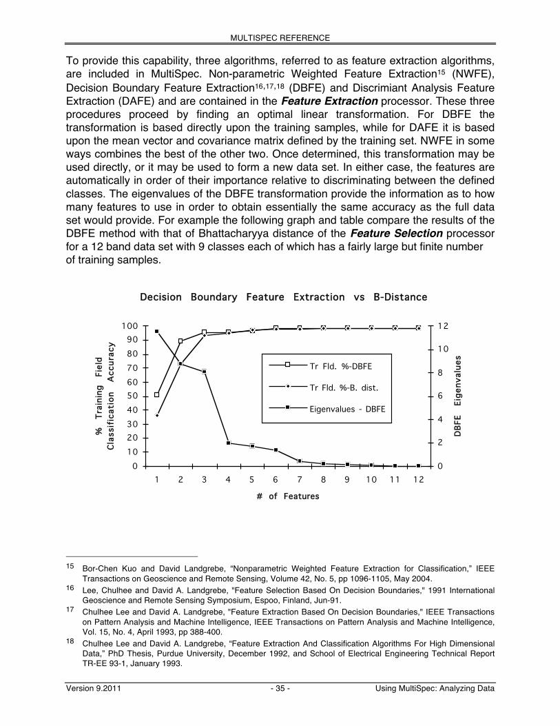
MULTISPEC REFERENCE


To provide this capability, three algorithms, referred to as feature extraction algorithms, are included in MultiSpec. Non-parametric Weighted Feature Extraction15 (NWFE), Decision Boundary Feature Extraction16,17,18 (DBFE) and Discrimiant Analysis Feature Extraction (DAFE) and are contained in the Feature Extraction processor. These three procedures proceed by finding an optimal linear transformation. For DBFE the transformation is based directly upon the training samples, while for DAFE it is based upon the mean vector and covariance matrix defined by the training set. NWFE in some ways combines the best of the other two. Once determined, this transformation may be used directly, or it may be used to form a new data set. In either case, the features are automatically in order of their importance relative to discriminating between the defined classes. The eigenvalues of the DBFE transformation provide the information as to how many features to use in order to obtain essentially the same accuracy as the full data set would provide. For example the following graph and table compare the results of the DBFE method with that of Bhattacharyya distance of the Feature Selection processor for a 12 band data set with 9 classes each of which has a fairly large but finite number of training samples.

15 Bor-Chen Kuo and David Landgrebe, “Nonparametric Weighted Feature Extraction for Classification,” IEEE

Transactions on Geoscience and Remote Sensing, Volume 42, No. 5, pp 1096-1105, May 2004. 16 Lee, Chulhee and David A. Landgrebe, "Feature Selection Based On Decision Boundaries," 1991 International

Geoscience and Remote Sensing Symposium, Espoo, Finland, Jun-91. 17 Chulhee Lee and David A. Landgrebe, "Feature Extraction Based On Decision Boundaries," IEEE Transactions

on Pattern Analysis and Machine Intelligence, IEEE Transactions on Pattern Analysis and Machine Intelligence, Vol. 15, No. 4, April 1993, pp 388-400.

18 Chulhee Lee and David A. Landgrebe, “Feature Extraction And Classification Algorithms For High Dimensional Data,” PhD Thesis, Purdue University, December 1992, and School of Electrical Engineering Technical Report TR-EE 93-1, January 1993.

Decision Boundary Feature Extraction vs B-Distance

# of Features

%

Trai

ning

Fi

eld

Clas

sifi

cati

on

Acc

urac

y

0102030405060708090

100

1 2 3 4 5 6 7 8 9 10 11 120

2

4

6

8

10

12

DBF

E Ei

genv

alue

s

Tr Fld. %-DBFE

Tr Fld. %-B. dist.

Eigenvalues - DBFE

MULTISPEC REFERENCE


Dimension 1 2 3 4 5 6 7 8 9 10 11 12 Eigenvalues - DBFE 11.569 8.7917 8.0953 1.9662 1.7316 1.3462 0.4323 0.2004 0.1744 0.0829 0.0327 0.0164 Tr Fld. %-DBFE 50.9 89.4 95.5 95.8 97.0 98.4 98.4 98.4 98.4 98.5 98.5 98.5 Tr Fld. %-B. dist. 36.2 72.9 93.5 94.8 97.2 97.8 98.0 98.2 98.3 98.4 98.4 98.5 Tr Fld. %-DAFE 64.1 87.4 96.0 97.4 97.8 98.1 98.4 98.4 98.5 98.5 98.5 98.5

Activation of the DBFE algorithm causes calculation of the data such as that labeled Eigenvalues - DBFE in the above table. The relative size of each eigenvalue is proportional to that featureʼs discrimination value. Thus in this case, by comparing the size of these entries, one concludes that the first three features should provide most of the available separability, adding three more should provide a small amount in addition, and the remaining ones should contribute very little. The line of the table labeled Tr Fld. %-DBFE shows the results obtained by classification verifying this. The line labeled Tr Fld. %-B. dist. shows the corresponding results using the Bhattacharyya Distance option of the Feature Selection processor. The final line of the table gives the corresponding classification results for the DAFE procedure, showing very similar performance. These data show that, not only do the DBFE and DAFE features equal or exceed those of B-distance in accuracy, but they tend to provide better separability at a lower dimensionality. Further, the eigenvalues resulting from the DBFE show just how many features to use, while the B-distance method gives very little information on this point. Thus the guess-work and art needed in effective feature selection is reduced.

The theoretical basis for the DBFE algorithm is to use the decision boundary location of each class pair to determine “discriminately informative” and “discriminately redundant” features. A brief outline of the steps it follows are:

1. Classify the training samples of the first class pair. 2. For pixels of class 1 locate the nearest pixel of class 2, and from this locate a

point on the decision boundary that is on the line segment between them. After this is done for all the training samples, the effective portion of the entire decision boundary is determined.

3. From this, determine a “Decision Boundary Feature Matrix” which contains the essential information about how to form discriminately informative features.

4. Repeat this process for all class pairs and form the (possibly weighted) sum of the resulting Decision Boundary Feature Matrices. A possible additional step can optimize the transformation by eliminating some redundancy, making it more efficient.

The DAFE algorithm is a more standard discriminant analysis algorithm based on within-class and between-class scatter matrices. The advantage of the DAFE algorithm is that it is fast, but it does not tend to perform will in cases where the classes involved have a small difference in mean values. Further, it only provides features reliably up to one less than the number of classes involved.

MULTISPEC REFERENCE


DBFE does not have these disadvantages, but it is a much longer calculation and it does not perform as well with small training sets. More details about it are given in the Feature Extraction portion of the Reference section of these notes. NWFE was developed by Dr. Bor-Chen Kuo. It is based on a non-parametric extension of scatter matrices. There are at least two advantages to using NWFE non-parametric scatter matrices. First, they are generally of full rank. This provides the ability to specify the number of extracted features desired and to reduce the effect of the singularity problem. This is in contrast to parametric discriminant analysis (DAFE), which usually only can extract L-1 (number of classes minus one) features. In a real situation, this may not be enough. Second, the non-parametric nature of scatter matrices reduces the effects of outliers and works well even for non-normal data sets. The new method provides greater weight to samples near the expected decision boundary. This tends to provide for increased classification accuracy. This algorithm has been found to be useful for higher dimensional data when a limited number of training samples are available. The steps needed to use any of these algorithms are as follows:

1. After selecting the training set, choose Nonparametric Weighting, Decision Boundary or the Discriminate Analysis option from the Feature Extraction menu. One may choose unequal class weighting and, for the DBFE case, unequal interclass weighting at this point if desired. For the DBFE case, there are also some “special options” available for users who become more familiar with the details of the algorithms via the references. For most uses, the default options should be satisfactory, and so simply click OK.

2. Upon completion of the calculation resulting from this processor, the

necessary transformation data is presented in the text window and stored in memory. At this point, if desired, one may select the “Use Feature Transformation” check box near the Channels pop-up box and proceed normally with any of the four functions for which such statistics are used, i.e., Classify, Feature Selection, Create Statistics Image, Check Covariances. If DBFE is being used, use the first N features, where N may be selected from the list of eigenvalues as indicated above.

3. If repeated use of the transformed statistics are envisioned, then the

transformed statistics may be saved via the Save Transformation as... item on the File menu, or it may be desirable to create a new data file based upon the transformed data. To do so, choose the Change Image File Format from the Reformat processor, and click on the Transform data ... check box in the ensuing dialog box. Select the New channels from Eigenvectors option in the resulting dialog box and note the recommended number of bits. After selecting OK, set the number of bits per data value to at least the number recommended in order to ensure that adequate dynamic range will be available for the transformed data. The user may want to select a subset of features as desired in the new file, as this can reduce the size of the file

MULTISPEC REFERENCE


significantly. Upon clicking OK the new data set will be created. Display the new image and select the Change Base Image File item from the Project menu to change the base image to the newly created transformed data. This data set may then be classified in the normal way, however, by examining the eigenvalues shown in the text window after step 1, one can choose which features to use, based upon the relationship of eigenvalue size to accuracy discussed with regard to the above table.

For users with an interest in the mathematical details, a more complete development of the theory and some example test results for DBFE are given in the references cited above19. The problem becomes even more complex for hyperspectral data, since NWFE, DAFE and DBFE calculations begin with computation in the full dimensional space in order to find the optimal transformation to a lower dimensional space. Thus these calculations, too, may suffer from small training set situations. To deal with this limitation, a class-conditional pre-processing algorithm was designed based upon a method known as projection pursuit20,21. This algorithm does the necessary calculations in the projected space, rather than the original, high dimensional space. The figure below shows the overall scheme. The data at point Φ might be 200 dimensional. Through projection pursuit, a subspace of perhaps 20 dimensions might be determined, and in this case, all calculations are done at a dimensionality of 20. This can then more optimally be followed by NWFE, DAFE or DBFE to find a subspace of perhaps 10 dimensions in which to do the classification. In this way, maximal advantage can be taken of a training set of limited size.

19 We note in passing that though the DBFE algorithm has been used here only in its parametric form, it has been

generalized to nonparametric classifiers as well. See: -Chulhee Lee and David A. Landgrebe, "Decision Boundary Feature Extraction for Non-Parametric

Classification," IEEE Transactions on System, Man, and Cybernetics, Vol. 23, No. 2, March/April, 1993, and, -Chulhee Lee and David A. Landgrebe, “Decision Boundary Feature Extraction for Neural Networks,” IEEE

Transactions on Neural Networks, Vol. 8, No. 1, pp 75-83, January 1997. 20 Luis Jimenez and David Landgrebe, “Projection Pursuit For High Dimensional Feature Reduction: Parallel And

Sequential Approaches,” Presented at the International Geoscience and Remote Sensing Symposium (IGARSS'95), Florence Italy, July 10-14, 1995.

21 Luis Jimenez and David Landgrebe, “Projection Pursuit in High Dimensional Data Reduction: Initial Conditions, Feature Selection and the Assumption of Normality,” IEEE International Conference on Systems, Man, and Cybernetics, Vancouver, Canada, October 22-25, 1995.

MULTISPEC REFERENCE


Classification of high dimensional data including reprocessing of high dimensional data. The projection pursuit algorithm used to accomplish the preprocessing step is accessed in the Feature Extraction processor. Choosing this processor allows for the direct use of DAFE or DBFE, or to precede this with the use of Projection Pursuit preprocessing. The latter is primarily intended for cases where hyperspectral data is involved. BiPlot Of Data (Macintosh version only) One can make scatter plots of selected areas and pairs of channels of data. One can create a biplot of training data, test data and selected areas. This capability is available under the Utilities submenu under the Processor Menu item. This processor also can draw the ellipses of concentration representing the class statistics on the biplot graphs. An example of these plots is given below showing the ellipse of concentration of class 3 compared to the scatter plot of pixels from one field of that class. The ellipse plots represent the ellipse for the data projected onto the requested

plane. One can control the size of the ellipse by setting the desired threshold level in percent. One can plot the data values and ellipses in transformed space by selecting the 'Use Transformation' check box in the Biplot Dialog window. If a transformation is applied to the data, 'Feature' will be used as the abscissa label on the graphs; if the original data is being plotted then 'Channel' is used for the label.

Class Conditioned Pre-processing

High Dimensional Data

Classification/AnalysisFeature Extraction

Dimension Reduced

Dimension Further Reduced

Sample Label Information

!" # $

144146148150

152

100 110 120 130 140 150

BiPlot of Channels 7 vs 4

Channel 4

Channel 7

+++ +++

+++++ +++

+++ +++

++

+ ++

++

++

++

+++ + ++ +++ +

+ + ++++++++

+ ++++

+++

+++

++

++ + +++

+++

+++

++++++

++++

++ +

+++++++ + +

+++ + ++++ +++++ ++

++

++ ++ ++ ++

+

MULTISPEC REFERENCE


Spectral Graph. One may display a graph showing how the gray level digital count values vary from spectral band to spectral band for a given pixel. This capability is activated by choosing New Selection Graph from the Window menu. This causes a window to be opened displaying the graph. Selecting a single pixel results in its spectrum being graphed. If the selection represents more than one pixel in multispectral image windows, the average, plus and minus one standard deviation and the minimum and maximum values are plotted in the selection graph. An example of such a graph for a 191 band pixel is shown to the right. This graph is useful in judging the relative signal level in the various bands. Graph windows can be printed or copied to the clipboard. A graph window will be copied just as it is on the screen. The graph can then be copied into another application such as a word processor. To copy a graph window, make it the active window and then use the Edit menu item Copy or COMMAND-C. If one is displaying graphs within the ListData processor then one must use COMMAND-C to copy the graph window.

Statistics Image Display (Macintosh version only) One may also create a display showing both the first and second order statistics of classes or fields.22 This form of display is most useful in color. To illustrate, the two examples below compare the statistics for two classes in 12 bands. The large square consisting of 12 by 12 smaller squares in the upper portion of this display depicts the correlation matrix of the classes. Each individual small square shows the relative degree of correlation for one particular band to another, on a scale from blue (≈ -1) to green (≈ 0) to red (≈ +1), as indicated by the color bar at the very bottom. Bands are indicated by the row and column number. For example, the square in the first column of the eleventh row shows the correlation between bands one and eleven to be near zero. To the right and also below the square of squares the wavelengths are indicated if this data has been entered into the data file. The lower portion of the display shows a graph of the variation of the mean value ±1σ versus the band number.

22 Chulhee Lee and David A. Landgrebe, "Analyzing High Dimensional Multispectral Data, IEEE Transactions on

Geoscience and Remote Sensing, Volume 31, No. 4, pp 792-800, July 1993.

MULTISPEC REFERENCE


Water

Wheat

These Statistics Image plots are perhaps most useful for high dimensional data, where visualization of the statistical variation present in a class is more difficult to perceive. Shown below are example displays for two classes of AVIRIS data containing 210 bands. The Statistics Image displays in this case graphically reveal that the two classes have very different second order statistics, even in spectral ranges where the first order statistics (the mean values) are similar, and thus the two classes should be relatively separable. Statistics Image displays may be created by choosing Create Statistics Image… from the Utilities item of the Processor menu. A dialog box will then allow one to select several parameter values, including which bands and which classes

Class 1

Class 2

or fields one wishes to include, after which a new file is created containing the Statistics Image in the same format as a Thematic image. This file may be opened and displayed in the usual manner.

MULTISPEC REFERENCE

Version 9.2011 - 42 - Reference: MultiSpec Windows

IV. MultiSpec Reference The reference provides detailed information about:

- MultiSpec Windows, - MultiSpec Menu Items, - Shared Dialog Boxes and - General Characteristics of MultiSpec

Most of the pictures of windows and dialog boxes are taken from the Macintosh version running under Mac OSX. Figures are included for those windows and dialog boxes in the Windows version which differ significantly from those in the Macintosh version. The pictures for the Windows version were taken from the 32-bit Windows version running under Windows NT 4.0.

MultiSpec Windows This section describes the windows that are used in MultiSpec. There are:

- an output text window, - image windows of two types

- multispectral image window - thematic image window

- a project window - graph windows of three types

- selection graph window - biplot graph window - histogram graph window

- a coordinate view The output text, image and graph windows can be printed as described under the “File – Print…” menu item. Also these three types of windows can be copied as described under the “Edit – Copy” menu item. Each of the windows are shown and described below. First, those controls that are shared across several different types of windows are described.

MULTISPEC REFERENCE


Shared Window Controls This section describes the controls on a window that are shared across the different types of windows used in MultiSpec.

Macintosh Version

Windows Version

Close button

Collapse window button

Window zoom button

Window Title

Dragging portion control

Arrow scroll control

Space in scroll bar

Thumb scroll control

Window sizing box

Window Title

Dragging portion control

Collapse window box

Expand window box

Close box

Arrow control

Space in scroll bar

Thumb scroll control

Window sizing box

MULTISPEC REFERENCE


Close box: This control button closes the window. It does the same operation as the ‘File-Close Window’ menu item. Window title: This is the title for the window. One can click the mouse button down on or near the title to move the window to another location on the monitor or to another monitor if attached. Window zoom box: (Macintosh version only) This control button will force the edge of the window to just fit around the image being displayed in the window. If one then clicks in this box again, the edge of the window will go back to its original size. Collapse window box: This control button collapses the window to be just the title. If one clicks on the box again, the full window will be displayed again. Expand window box: (Windows version only) This control button expands the size of the window to fit the entire application main window. If one clicks on the box again, the window will be displayed at its previous size. One can view more than one window at a time within the MultiSpec application window. Scroll controls: One can scroll the text or image if it is larger than the window by using the horizontal and vertical scroll bars along the window edge.

Arrows: Click on the up, down, left or right arrows to scroll a line of text or a small portion of the image at a time. Thumb: Click the mouse button down on the thumb control and then move it to the desired location. When one lets the mouse button up, the text or image will scroll to that location. Space scroll bar: One can click the mouse button down on the space on either side of the thumb to scroll a “page” of text or image at a time.

Dragging edge control: Clicking the mouse button in the title (and also along the edge for Windows version) allows one to move the image window to another location on the monitor or to a second monitor if attached. Window sizing box: This control allows one to change the size of the window. The procedure is to move the cursor over this box, click the mouse button down and then drag the lower right corner of the window to the desired size.

MULTISPEC REFERENCE

Version 9.2011 - 45 - Reference: Output Text Window

Output Text Window The output text window is created when MultiSpec is opened. All text output from MultiSpec’s processors is written into this window. The text in the window will summarize what the processor action did and include any tables such as a classification results summary. The Output Text Window

Hiding Window: The output text window cannot be closed. It can be hidden using the “Window-Hide Window” menu command. Saving Window: One can save the information (or selected information) in the text window to a disk file using the “File-Save Text Output As …” menu command. One will also be prompted to save the information in the text output window when one quits MultiSpec if the information in the window has changed since the last save operation. Copying Window: One can also copy the information in the window (or a selected portion of it) to the clipboard so that the information can be pasted into another application. Paste into Window: One can past information into the output text window. However one cannot open up a previously saved text output window with MultiSpec. If one wishes to do this, then open the previously saved disk file with a text editor application and then copy the text from that application to the output text window in MultiSpec.

MULTISPEC REFERENCE

Version 9.2011 - 46 - Reference: Image Windows

Image Windows

Image windows are created with the “Processor-> Display Image…” menu item. There are two types of image windows – multispectral image windows and thematic image windows.

- Multispectral image windows are used to display multispectral scanner data for which one wants to select the channels (or features) to be displayed as red, green, or blue.

- Thematic image windows are used to display classification output images or other Geographic Information System (GIS) raster images where specific colors in the image will be assigned to specific themes.

Multispectral Image Window (3-channel display)

Macintosh Version

Windows Version

Coordinate View control

Cursor (not shown)

Selected area

Overlay control

Zoom out control

Zoom in control

Zoom factor indicator

Tool Bar

Overlay control

Zoom out control

Zoom in control

Magnification control

Selected area

Zoom factor indicator

MULTISPEC REFERENCE


The window above is a multispectral image window. It represents a 3-channel color IR display of Thematic Mapper data. The title of the window includes the image file name that the image represents plus the channels that are used to display the image in red, green, blue order. Many of the control buttons on the window are described above under “Shared Window Controls”. The control buttons that are unique to image windows are described below. Coordinate view control (Macinstosh version only): This control button causes the coordinate view to be displayed above the image. If one clicks on the box again, the coordinate view will be closed. One can also display and close the coordinate view using the Window – Show/Hide Coordinate View menu item. Note for Windows version, one can Show/Hide the Coordinate View using the View - Show/Hide Coordinate View or Window – Show/Hide Coordinate View menu items. Cursor: The cursor is in the shape of a ‘+’ when it is over the image. In Macintosh version only: If one holds the option key down, the cursor will change to a hand. One can then mouse down on the image and drag or scroll the image in any direction. Selected area: This is an example of a selected area within the image. See the section below on “Making Selections within an Image Window”. Overlay control: This control button causes the popup menu to the right to be displayed. The popup menu allows one to control the visible status of any overlays assigned to the image window. One can hide all overlays (No overlays), show all overlays (All overlays), or hide/show an individual overlay. A checkmark indicates that the overlay is being drawn in the image window. If one holds the option key down (Macintosh version) or shift key down (Windows version) before mousing down in this control, the popup menu to the right is displayed. Upon selecting one of the overlays, one can select the color and thickness of the overlay lines using the 'Set Overlay Parameters' dialog box that is illustrated below.

MULTISPEC REFERENCE


If no overlays are assigned to the image window, this control is not drawn. Zoom out: This control allows one to zoom out of the image. Zoom in: This control allows one to zoom in to the image. If one clicks on the zoom in button, one will zoom in one step such as from x1.0 to x2.0 to x3.0, etc. The center point of the zoom may be controlled by selecting a point in the image, i.e. clicking on a point or selecting an area. The zoom in will then be centered as near as possible to that point or area. If one clicks on the zoom out button one will zoom out one step such as x2.0 to x1.0 to x0.5 (1/2) to x0.33 (1/3), etc. There are some options that can be used with the zoom control buttons.

- If one holds the ‘Option’ key (Macintosh version) or ‘Control’ key (Windows version) down when one clicks on one of the zoom buttons, the zoom factor will be by 0.1 steps instead of 1.0 steps.

- Also if one holds the zoom buttons down, the zooming action will be continuous at a rate of up to 3 or 4 steps per second. However, if one holds the command key (Macintosh version) or right mouse button (Windows version) down while holding the mouse button down within a zoom control button, the zooming action will be as fast as the computer can go.

Zoom Factor Indicator: The title of this control, currently x1.0, indicates to the user what the zoom factor is. It also allows one to go directly to the non-magnified state, i.e., X 1.0, if not already there by simply clicking on it.

MULTISPEC REFERENCE


Multispectral Image Window (side by side channel display)

The window above is another example of a multispectral image window. It represents three spectral channels displayed side by side using the "Side by Side Channels" Display Type option in the dialog box presented by the ‘Processor-> Display Image…’ menu item. The title above each of the channels represents the channel number and if available, the channel description. If the width of the channel is too narrow, only the channel number will be given. The controls around the window are the same as those discussed above. When one makes a selection within one of the channels, that selection will be drawn in all of the channels. The zooming operation will be centered around the channel that the selection was actually made in. Note that overlays are currently not drawn in "Side by Side Channels" image windows.

MULTISPEC REFERENCE


Multispectral Image Window (1-channel thematic display)

The window above is an example of a 1-channel thematic display of multispectral image data. It represents one spectral band displayed as a thematic image using the "1-Channel Thematic" Display Type option in the dialog box presented by the ‘Processor-> Display Image…’ menu item. This is useful to display "product" type images such as MODIS NDVI or any of the other many MODIS products. The data values are grouped into the desired number of levels and a legend is displayed to the left of the image indicating which palette colors are associated with each range of data. One can also enter a factor to use to multiply times the data values displayed in the legend to reflect the actual measurement value. Sometimes the data value may be the measurement value times 100 or 1000. One can use the Reformat-> Change Image File Format processor to create thematic images based on what is displayed in the image window. One can use the Min/Max User Specified dialog box item to set the min and max values for the range of data to be displayed. Black is the default color for data values less than the minimum and white is the default color for values greater than the maximum. Note: This feature can be considered as a supervised 1-channel levels classifier.

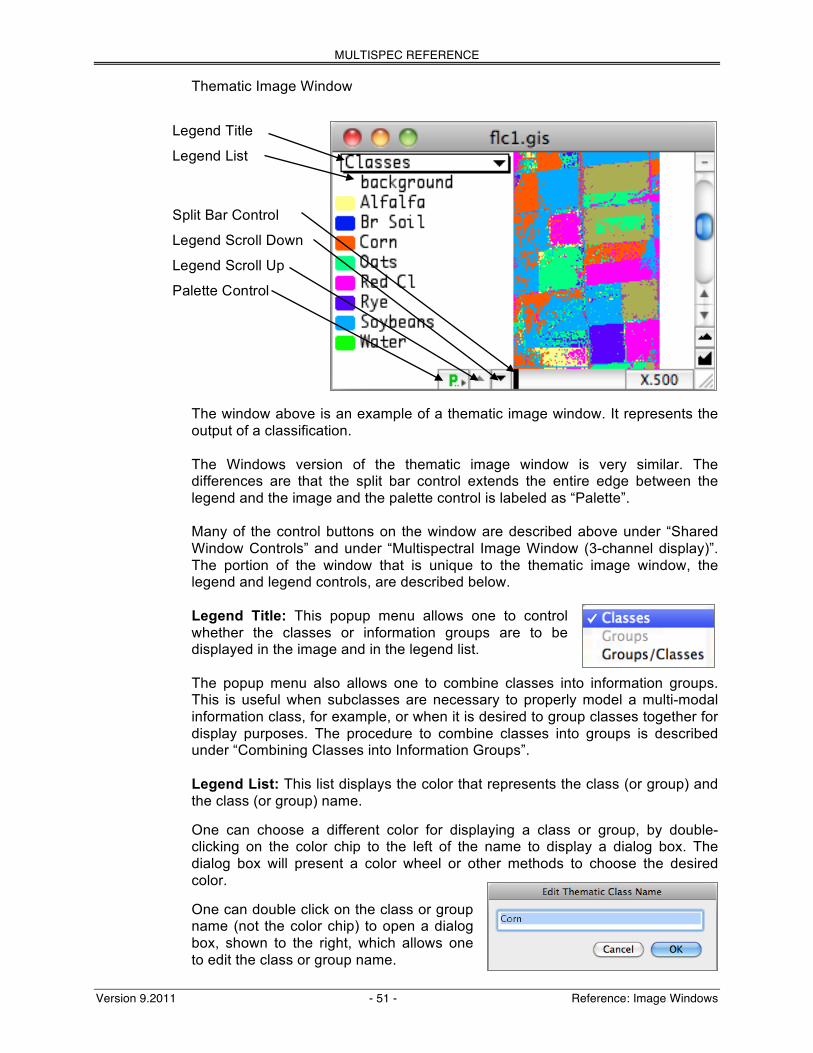
MULTISPEC REFERENCE


Thematic Image Window

The window above is an example of a thematic image window. It represents the output of a classification. The Windows version of the thematic image window is very similar. The differences are that the split bar control extends the entire edge between the legend and the image and the palette control is labeled as “Palette”. Many of the control buttons on the window are described above under “Shared Window Controls” and under “Multispectral Image Window (3-channel display)”. The portion of the window that is unique to the thematic image window, the legend and legend controls, are described below. Legend Title: This popup menu allows one to control whether the classes or information groups are to be displayed in the image and in the legend list. The popup menu also allows one to combine classes into information groups. This is useful when subclasses are necessary to properly model a multi-modal information class, for example, or when it is desired to group classes together for display purposes. The procedure to combine classes into groups is described under “Combining Classes into Information Groups”. Legend List: This list displays the color that represents the class (or group) and the class (or group) name. One can choose a different color for displaying a class or group, by double-clicking on the color chip to the left of the name to display a dialog box. The dialog box will present a color wheel or other methods to choose the desired color. One can double click on the class or group name (not the color chip) to open a dialog box, shown to the right, which allows one to edit the class or group name.

Legend Title

Legend List

Split Bar Control

Legend Scroll Down

Legend Scroll Up

Palette Control

MULTISPEC REFERENCE


Split Bar Control: One controls the width of the legend by mousing down on the split bar and dragging to the desired legend width. If one changes the width of the legend to less than 5 pixels wide, then no legend is displayed. Note that the width of the legend is forced to a minimum width so that the pop-up menu can be displayed. If one double clicks on the split bar while the legend is closed, the legend will automatically open. If the legend is open and one double clicks on the split bar, the legend will close. Legend Scroll Down/Legend Scroll Up: These control buttons allow one to scroll the legend list down or up. The list will scroll slowly enough to allow one to read the list. If one wants to scroll as fast as possible, hold the command key down while holding the mouse down on the control button. One can also scroll the legend list down by holding the mouse button down when the cursor is over the list and dragging the cursor below the bottom of the list or above the top of the list. Palette Control: This button allows one to choose the color palette to be used. Selecting the button will display the popup menu to the right. There is a default set of colors and gray levels. The Blue-Green-Red palette is one with a fairly smooth (subtle) transition from one color to the next, i.e. from one class to the next. This is used to create Statistics Images. The AVHRR NDVI and MODIS NDVI are a special sets for those types of images. When one selects 'False Color...' a dialog box will appear which allows the user to select the channels in each class mean vector to define the red, green and blue value for each thematic color. Note that an open project file is required for this option. See the description for the ‘Assign Channels for False Color Palette’ dialog box under the Shared Dialog Boxes section.

MULTISPEC REFERENCE


Combining Classes into Information Groups It may be useful to combine classes in a thematic image into information groups when subclasses are necessary to properly model a multi-modal information class, for example, or when it is desired to group classes together for display and/or informational purposes. Doing so allows a thematic image to be displayed in terms of information groups, and classification accuracy can be evaluated in terms of information groups as well. This grouping is accomplished when viewing a thematic image. A group may be defined by mousing down on the Classes popup menu and sliding to Groups/Classes. The legend will be displayed as shown immediately to the right. To move a class (the numbered items) into another group (the unnumbered items), simply drag the class to the desired group, e.g. drag 2-Alfalfa to 6-Red Clover. The Group "Forage" will then have two members as shown in the legend displayed on the far right. Note that the group name was changed from “Red Clover” to “Forage” as described in the next paragraph. One can double click on the group name (not the color chip) to open a dialog box which allows one to edit the group name. For the case above the group name was changed from ‘Red Clover’ to ‘Forage’. Note that the color chip in the Group/Class list goes with the group names. List items without color chips represents classes. If one holds the control key down and double clicks on a class name, the class will be assigned to a new group. A dialog box will appear allowing one to enter the name for the new group.

MULTISPEC REFERENCE


Other User Actions on Thematic Legends Save Changes: One can save changes in the class or group names and assigned colors by selecting 'Save Thematic Class/Group Info As...' from the File menu. The changes can be saved to the current trailer file associated with the class. The default name for this file is the image name with .TRL suffix. Alternatively, one can save to a different file. A different trailer file that contains the class names and colors can be associated with the thematic image by selecting 'Open Thematic Class Info...' from the File menu. Blink Class or Group Colors: One can 'blink' the class or group by placing the cursor over the respective color chip in the Legend (both Macintosh and Windows versions) or over the respective color in the image window (Macintosh version only) and do the following:

Shift Key: If one holds the shift key down, the cursor will change to an eye. Clicking the mouse button down will change the color of the class or group to the background color. Releasing the mouse button will change the color back to the original. Shift and Control Keys: If one holds the shift and control keys down, the cursor will change to an eye. Clicking the mouse button down will change the color of all of the other classes or groups to the background color. Releasing the mouse button will change the colors back to the original. Shift and Option Keys: (Macintosh version) Shift and Right Mouse Button: (Windows version) If one holds these keys or buttons down, the cursor will change to an eye. Clicking the mouse button down will change the colors of this class or group and all with class/group numbers less than the selected one to the background color. Releasing the mouse button will change the colors back to the original23.

23 This capability was really implemented for Probability Images. See the section on the Classify selection of the

Processor menu.

MULTISPEC REFERENCE


Selections within an Image Window Uses for Selected Areas: Selected areas are used for:

- Defining areas to be used as training and or test fields. This is described under the “Select Field Project Window”.

- Defining areas within which a processor function is to operate on. Many processor functions such as “Histogram Image…” and “List Data…” have dialog boxes which allow one to specify an area in the image file to use. If a rectangle selection is made in the image window, this is the area that is used as the default in these dialog boxes. The dialog boxes also have a button to allow one to quickly change the selected area to the entire area in the image file. This button does not affect the selected area in the image window.

- Define an area to zoom in on. This is described under the discussion of the “Zoom in” control button above.

Making Selections: One can make selections within an image window by mousing down on a corner and dragging diagonally to the opposite corner of the area that one wishes to select. The area is selected when one releases the mouse button. This action will cause the area to be outlined in the image window with a dashed line. If one drags to the edge of the window during a rectangle selection, the image will automatically scroll to show a new portion of the image window if it is not currently at the edge of the image. If the coordinate view is visible, the coordinates of the selection will appear in it along with the number of pixels in the selected area. Deleting Selections: Selections in the active image window can be deleted by using the “Edit – Clear Selection Rectangle” menu item or by striking the delete key. Duplicate Selections in all Image Windows: One can also cause a selection in one image window to be applied to all open image windows. To do this, hold the control key down while making the selection. The temporary selection will be drawn (and redrawn) in the active image window. When the mouse button is released, that selection will be converted to a permanent selection (dashed lines) in all image windows. Note that the control key needs to be down when the mouse button is released to cause the above to happen. If the coordinate view is open, then the units used for making the selection in the open image windows will be that selected in the coordinate view - lines/columns, degrees or map units. This is a good way to make a selection of the same ground area in more than one image window when the image files do not represent the identical area on the ground. If the coordinate view is hidden, then lines/column units will be used for the duplicate selections in the open image windows. The start line and columns of each of the image windows and image files are taken into account.

MULTISPEC REFERENCE

Version 9.2011 - 56 - Reference: Project Window

Project Window The project window is created with the “Processor – Statistics…” menu item. The project window has four modes indicated by the name below the project name:

- The “SELECT FIELD” mode is used to select training and test areas for classes. - The “CLASS LIST” mode is used to list and operate on the classes in the project. - The “FIELD LIST” mode is used to list and operate on the fields within a given class. - The “COORDINATE LIST” mode is used to list and operate on the coordinates that

define a given field or area. The group of buttons near the center of the window labeled >Project, >Class, >Field, and >Select allow one to move from one mode to another.

The “SELECT FIELD” Project Window

As stated above, the “SELECT FIELD” mode is used to select training and test areas for project classes. The selected areas can be created in three ways:

- Rectangular areas can be selected as described under the “Selections within an Image Window” section above.

- Rectangular areas can be created using the “Edit Selection” button described below.

- Polygonal areas can be selected as described in the “Polygon Enter” discussion below.

Once a selection is made in a project image window, which may be the base image window or an associated image window (see the “Project – Add as Associated” menu item), the “Add To List…” button that is described below will be enabled.

MULTISPEC REFERENCE


More detailed information about the controls in the “SELECT FIELD” Project Window follows. Class: This popup menu allows one to select the class to which a selected field is to be assigned. If the current class name is “New”, then the selected field will be added to a new class which the user will be given the chance to name. See the “Add to List” button below. Polygon Enter: This check box allows one to select polygonal shaped areas instead of rectangular areas. In this case, fields are selected by clicking on the corners of the desired polygons, instead of dragging24. One completes the polygon selection by double clicking on the last point to be selected. While the polygon selection has not been completed, one can delete the last selected point by striking the delete key. Edit Selection: This button will cause a dialog box to be presented to allow one to enter or edit the line and column coordinates of the selected rectangular area. See the “Edit – Edit Rectangle Selection…” menu item for more information. Add To List…: This button will cause the “Define Class and/or Field” dialog box to be presented to allow one to add the selected area, referred to as a field, to the project. This dialog box allows one to associate the field to a class, name the field and define the field as being either a train or test field. The “Define Class and/or Field” dialog box is discussed in more detail below. This button can also be activated by striking the 'Return' or 'Enter' key when a selection has been made in an image window associated with the project and the Project window is in the ' SELECT FIELD’ mode. This action will work even if the image window is the active window. >Classes, >Fields, >Coord.: These buttons allow one to change the project window mode to CLASS LIST, FIELD LIST or COORDINATE LIST, respectively. Coordinates (L,C): This list includes the line and column coordinates for the corners or vertices of the selected area. A rectangular area is defined by the coordinates of the upper left and the lower right corners. Polygon areas are defined by the coordinates of each of the vertices of the polygon.

24 NOTE, a problem has been found with polygonal fields. The right most column and bottom most line will not be

included in a polygonal field as one might expect. An example to illustrate the problem is to select a rectangular field and a polygonal field of the same area. The polygonal field will not include the right most column or the bottom most line as are included in the rectangular field of the same specifications. This should be taken into account when selecting polygonal fields. A fix for this problem is not known at this time.

MULTISPEC REFERENCE


The “CLASS LIST” Project Window

The “CLASS LIST” mode is used to list and operate on the classes in the project. The “CLASS LIST” Project Window is shown to the right. More detailed information about the controls in the window follows. Edit Class Name…: This button causes a dialog box to appear to allow one to edit the class name. This dialog box is a subset of the “Define Class and/or Field” dialog box. Stats: This text information indicates which statistics are currently being used for the project. These are defined under the “Project – Use Original Statistics” menu item. Histogram Classes: This button allows one to list a histogram of the classes or fields in the output text window or to create a graph of those histograms in a histogram graph window. Activating this button will cause the popup menu shown below and to the right to appear. This popup menu allows one to directly create a histogram of the classes in the project or of the fields in the project. The “Histogram…” option will cause the “Set Specifications for Class/Field Histograms” dialog box (described below) to appear to allow one to change the default settings for these histograms. List Classes Stats: This button allows one to list the class and/or field statistics in the output text window. Activating this button will cause the popup menu shown below and to the right to appear. This popup menu allows one to directly list the class statistics, the class and field statistics or just the field statistics. The “List Stats…” options will cause the “Set Specifications for Listing Statistics” dialog box (described below) to appear to allow one to change the default settings for the list. Update P. Stats: This button allows one to cause the statistics for the project to be updated. The button is enabled when there has been a change in the training fields. >Select, >Fields, >Coord.: These buttons allow one to change the project window mode to SELECT FIELD, FIELD LIST or COORDINATE LIST, respectively. Classes: This list includes the names of the classes defined for the project. If the number of classes is too large for the space, one may use the elevator and arrows to the right to scroll the list. One can select a class name in the list and then the "->Field" button, to move to the Field List mode of the Project Window. One can also just double click on the class name to do the same operation.

MULTISPEC REFERENCE


The “Field List” Project Window The “Class” mode is used to list and operate on the fields in a defined class. The “Field List” Project Window is shown to the right. More detailed information about the controls in the window follows. Class: This text information indicates what the defined class is for which the fields are listed. Edit Field Name…: This button causes a dialog box to be presented to allow one to edit the field name. It is a subset of the “Define Class and/or Field” dialog box. Stats: This popup menu allows one to set the type of statistics to use for the class. The types are defined under the “Project – Use Original Statistics” menu item. Histogram Class: This button allows one to list a histogram of the class or fields in the class in the output text window or to create a graph of those histograms in a histogram graph window. Activating this button will cause the popup menu shown below and to the right to appear. This popup menu allows one to directly create histogram(s) of the class or fields in the class. The “Histogram…” option will cause the “Set Specifications for Class/Field Histograms” dialog box (described below) to appear to allow one to change the default settings. List Class Stats: This button allows one to list the class and/or field statistics in the output text window. Activating this button will cause the popup menu shown below and to the right to appear. This popup menu allows one to directly list the class statistics, the class and field statistics or just the field statistics. The “List Stats…” options will cause the “Set Specifications for Listing Statistics” dialog box (described below) to be presented to allow one to change the default settings for the list. Update C. Stats: This button allows one to update the statistics for the class. The button is enabled when there has been a change in the training fields. >Select, >Classes, >Coord.: These buttons allow one to change the window mode to SELECT FIELD, CLASS LIST or COORDINATE LIST, respectively. Fields: This list includes the names of the fields defined for the class. If the number of fields is too large for the space, one may use the elevator and arrows to the right to scroll the list. One can select a field name in the list and then the ">Field" button, to move to the Coordinate List mode of the Project Window. One can also just double click on the field name to do the same operation.

MULTISPEC REFERENCE


The “Coordinate List” Project Window The “Field” mode is used to list and operate on the coordinates that define a field. The “Coordinate List” Project Window is shown to the right. More detailed information about the controls in the window follow. Class: This text information indicates what class the defined field is in. Field: This text information indicates what the defined field is for which the coordinates are listed. Edit Coordinates…: This button causes a dialog box to be presented to allow one to edit the coordinates for the field. Histogram Field: This button allows one to list a histogram of the class or fields in the class in the output text window or to create a graph of those histograms in a histogram graph window. Activating this button will cause the popup menu shown below and to the right to appear. This popup menu allows one to directly create a histogram of the field. The “Histogram…” option will cause the “Set Specifications for Class/Field Histograms” dialog box (described below) to appear to allow one to change the default settings for the histogram. List Field Stats: This button allows one to list the field statistics in the output text window. Activating this button will cause the popup menu shown below and to the right to appear. This popup menu allows one to directly list the field statistics. The “List Stats…” options will cause the “Set Specifications for Listing Statistics” dialog box (described below) to be presented to allow one to change the default settings for the list. Update F. Stats: This button allows one to cause the statistics for the field to be updated. The button is enabled when there has been a change in the training field. >Select, >Classes, >Fields: These buttons allow one to change the window mode to SELECT FIELD, CLASS LIST or FIELD LIST, respectively. Coordinates (L,C): This list includes the line and column coordinates for the corners or vertices of the field. If the number of coordinates is too large for the space, one may use the elevator and arrows to the right to scroll the list. If one double clicks on a line-column coordinate value, the “Edit Rectangular Field Coordinates” or “Edit Polygonal Field Coordinate” dialog box will appear to allow on to change the coordinates.

MULTISPEC REFERENCE


Cutting and Pasting Classes or Fields A field or a class can be cut and pasted into another class. Also by cutting and repasting, the order of the classes can be changed, since a repasted field or class is always added to the end of the current list. Cutting and pasting a field or a class in a project window is described under the “Edit” menu.

MULTISPEC REFERENCE


The Define Class and/or Field Dialog Box

Class: This popup menu allows one to select the class to associate the newly defined field. If the class name is “New”, the “Enter Class Name” edit box will appear to allow one to enter the class name. Enter Class Name: This edit box allows one to enter the name for the class. The default name is ‘Class’ plus the class number. The limit for the number of characters in the name is 31. Number train pixels in class: This text information indicates how many training pixels represent the class (including the field to be added if a training field). Enter Field Identifier: This edit box allows one to enter the name for the field. The default name is ‘Field’ plus the field number. The limit for the number of characters in the name is 31. Number pixels: This text information indicates how many pixels are in the field to be added to the project. Training Field/Test Field: These radio buttons allow one to define the field as being a training or test field for the class. Cancel: This button closes the dialog box and cancels the “Define Class and/or Field Description” request. OK: This button closes the dialog box and adds the selected field to the project. The selected field will be outlined as defined for a project field and the selection area will be removed to be ready for a new selection.

MULTISPEC REFERENCE


The Set Specifications for Class/Field Histograms Dialog Box

Classes/Fields: These radio buttons allow one to choose whether the histograms should be created for the class(es) or individual field(s). Use feature transformation: This checkbox allows one to specify whether the data for the original channels (unchecked) or the transformed channels (checked) are to be used to create the histograms. This option is only available if a transformation matrix is available by running a principal component analysis, a feature extraction analysis or reading a transformation from a disk file that has been previously saved by MultiSpec. Channels/Features: This popup menu allows one to choose to use all or a subset of the available channels (original channels) or features (transformed channels) in the project statistics. Output: These radio buttons allow one to select whether the histogram table should be listed in the output text window or plotted in a graph window.

Include empty bins: This check box allows one to request that empty bins in the histogram be included in the table listed in the output text window. Blank values outside of range: This check box allows one to request that bins outside of the minimum/maximum value be blank instead of having 0’s. Overlay density functions: This check box causes a density function to be drawn over the histogram.

Line/Column interval: These edit boxes allow one set the line and column interval when reading the data from the image file.

MULTISPEC REFERENCE


Output Options:

Group by: These radio buttons allow one to choose to group the information in the table by channels or by classes/fields. List format: These radio buttons allow one to choose to list the histogram table in a matrix or column format.

Cancel: This button closes the dialog box and cancels the “Histogram” request. OK: This button closes the dialog box and executes the “Histogram” request using the parameters set in the dialog box.

MULTISPEC REFERENCE


The Set Specifications for Listing Statistics Dialog Box

List Statistics For: These check boxes allow one to specify whether the class and/or field statistics are to be listed. Other Options:

Mean and Std. Dev. precision: This edit box allows one to specify the number of decimal digits to be included after the decimal point for the mean and standard deviation vectors. Covariance/Correlation precision: This edit box allows one to specify the number of decimal digits to be included after the decimal point for the covariance or correlation matrix elements. Use feature transformation: This checkbox allows one to specify whether the statistics for the original channels (unchecked) or the transformed channels (checked) are to be listed. This option is only available if a transformation matrix is available by running a principal component analysis, a feature extraction analysis or reading a transformation from a disk file that has been previously saved by MultiSpec.

Include: These check boxes allow one to specify whether the mean and standard deviation vectors, covariance matrices and/or correlation matrices are to be listed for the specified classes and/or fields. Cancel: This button closes the dialog box and cancels the “List Statistics” request. OK: This button closes the dialog box and executes the “List Statistics” request using the parameters set in the dialog box.

MULTISPEC REFERENCE

Version 9.2011 - 66 - Reference: Graph Windows

Graph Windows There are three types of graph windows – selection, biplot and histogram.

- Selection graph windows display response versus channel plots for selected areas in the image window.

- Biplot graph windows display a plot of the data for one channel (or feature) versus that of another.

- Histogram graph windows display histograms of data for selected classes or fields. Selection Graph Window This graph window is created by the “Window – New Selection Graph” menu item. If the selected area in a multispectral image window or thematic image window includes only one pixel, then the graph that is generated contains a single line (or ‘+’) which represents the data values for that pixel. If the selected area in a thematic image window includes more than one pixel, then the graph that is generated contains a ‘+’ which represents the data value for the upper left pixel of the selection. If the selected area in a multispectral image window includes more than one pixel, then the graph below is generated which includes multiple lines representing the average, plus/minus one standard deviation, and the minimum/maximum data values.

The control buttons on the window are described above under “Shared Window Controls”. Graph Title: The title of the graph indicates the selected lines and columns for the data values that the plots represent. Red line: The red line represents the average of the data values for each channel. Green lines: The green lines represent plus and minus one standard deviation away from the average of the data values for each channel. Blue lines: The blue lines represent the minimum and maximum data value for each channel.

Graph Title

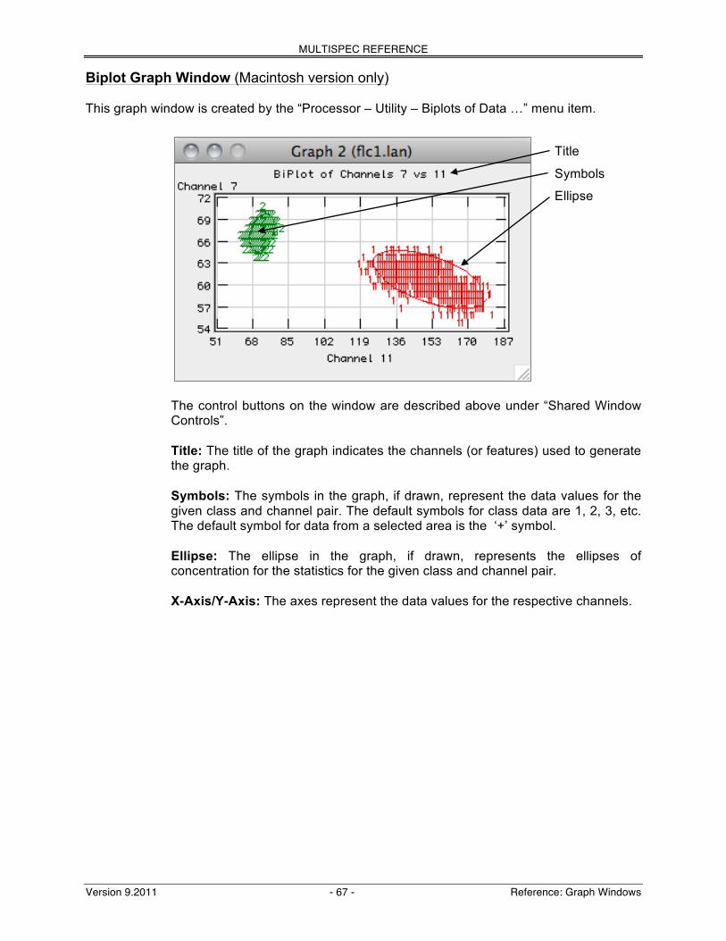
MULTISPEC REFERENCE


Biplot Graph Window (Macintosh version only) This graph window is created by the “Processor – Utility – Biplots of Data …” menu item.

The control buttons on the window are described above under “Shared Window Controls”. Title: The title of the graph indicates the channels (or features) used to generate the graph. Symbols: The symbols in the graph, if drawn, represent the data values for the given class and channel pair. The default symbols for class data are 1, 2, 3, etc. The default symbol for data from a selected area is the ‘+’ symbol. Ellipse: The ellipse in the graph, if drawn, represents the ellipses of concentration for the statistics for the given class and channel pair. X-Axis/Y-Axis: The axes represent the data values for the respective channels.

Title

Symbols

Ellipse

MULTISPEC REFERENCE


Histogram Graph Window This graph window is created by the “Histogram” button in the “Project Statistics”, “Class Statistics” and “Field Statistics” windows.

Many of the control buttons on the window are described above under “Shared Window Controls”. Those that are unique to the histogram graph window are described below. Title: The title of the graph indicates whether the histogram is for classes or fields and identifies the channel (or feature). Legend: The legend identifies the classes or fields whose histogram(s) are presently being displayed by color. Histogram: The vertical lines indicate the count for each data value. Density Function: The curve represents the Gaussian density function for the given class and channel. Channel scroll up/Channel scroll down: These control buttons allow one to change the channel (or feature) being displayed either up or down. The ‘scroll’ is implemented to allow no more than about two or three graph changes per second. If one holds the 'command' key down while one scrolls, the graphs will change as fast as the computer can draw them. This is helpful when one is viewing histograms of hyperspectral data. Legend control: This control button allows one to select the classes or fields being display in the graph. Overlay control: This control button allows one to select whether the density function and/or histogram is displayed in the graph. Bin width control: This control button allows one to control how many data values are to be represented by each bin. In the example graph above each data value is represent by a single bar.

Title

Legend

Histogram

Density Function

Channel scroll up

Channel scroll down

Legend control

Overlay control

Bin width control

MULTISPEC REFERENCE

Version 9.2011 - 69 - Reference: Coordinate View

Coordinate View The coordinate view is used to display the line and column location of the cursor within the image and the line and column coordinates of any selected area within the active image window. The number of pixels within the selected area is also displayed. The coordinate view is position just above the image in the image window. The Coordinate View (Macintosh version)

The coordinate view is created by the “Window – Show Coordinate View” menu item or selecting the coordinate view button above the vertical scroll bar.

The Coordinate View (Windows version)

The coordinate view is created by the “View-> Coordinates Bar” menu item or by the “Window-> Show Coordinate View” menu item.

MULTISPEC REFERENCE

Version 9.2011 - 70 - Reference: Coordinate View

Description of Elements in the Coordinate View Lines/Column Popup Menu: This popup menu, illustrated to the right, allows one to choose the units to be displayed for the cursor and selected area locations. Map projection information for the image is required to be able to use Lat-Long units or map distance units (Kilometers to Inches). Cursor Location: The cursor location is just to the right of the popup menu. The upper numbers represent vertical (line) information and the lower numbers represent horizontal (column) information. The units that may be selected depend upon the map information that has been defined for the image. Selected Area Location: The selected area is to the right of the cursor location after the vertical separator line. The upper numbers represent vertical (line) information and the lower numbers represent horizontal (column) information. For polygonal selections, the vertical and horizontal information represent the smallest rectangle than includes the selected polygon area. The units that may be selected depend upon the map information for the image. Number Pixels Popup Menu: This popup menu, shown to the right, allows one to select the units for the area of the selection. This may be how many pixels are included in the selection or the number of square kilometers, etc. Scale: This text information indicates the approximate scale of the image on the screen. This information is displayed if map information for the image is available and the units for the map information is given. The scale is approximate since a fixed value is used for the resolution of the monitor. The actual resolution of the monitor may differ from this fixed value.

Note: The thousands and decimal separators in the values in the coordinate view are those defined by the user for the operating system that they are using. Both the Mac and Windows OS allow one to set these according to the usage that the user desires. This must be done before MultiSpec is started.

MULTISPEC Reference

Version 9.2011 - 71 - Reference: File Menu

Menu Items The MultiSpec Application Menu (Macintosh OSX Version Only) About MultiSpec This menu item displays the version number and date of the MultiSpec application being used. The menu item also displays the Purdue Research Foundation copyright statement. One can also hide all MultiSpec windows or all other applications windows from this menu The Quit MultiSpec menu item allows one to quit MultiSpec. The File Menu The File Menu handles opening, loading, saving, and printing capabilities for image files and other supporting files. “File-> New Project” Menu Item This menu item causes a new project to be opened for the active image window. The Project Window will be displayed on the right portion of the monitor. Usually, the next step will be to select the Statistics... or Cluster... menu items under the Processor menu. In fact one can skip selecting the 'New Project' step and instead select the Statistics... or Cluster... menu items. If a project is not open, the action of selecting the 'Statistics...' or 'Cluster...' items will cause a new project to be opened for the active image window. “File-> Open Image” Menu Item

This menu item displays a dialog box to allow the user to select an image to be displayed. The dialog box, shown below, contains a list of those files on the current disk that may be image files plus all folders within the current folder. Macintosh version: All files for which MultiSpec recognizes the format will be high lighted in the open file dialog box as candidate image files. One has the option in the “Open Image File” dialog box files to high light all files. See Appendix E for information on how MultiSpec has specific image data formats.

MULTISPEC Reference


The Select Image Dialog Box

The Select Image dialog box behaves as the standard open file dialog box under Mac OSX or Windows operating systems. One can select the volumes or drives and folders to search for and select image files in. Enable: The enable popup menu, shown to the right, allows one to control which files can be selected … either all files that MultiSpec recognizes the file format of (the default), just known multispectral image files, thematic image files, shape files or all documents. Open image as: These radio buttons define how MultiSpec is to treat the image file - as a Multispectral image or as a Thematic image:

- For default case, MultiSpec will determine how to treat the image file by interpreting the header information in the file if available.

- Multispectral type images are usually selected for multispectral scanner data for which one wants to select the channels to be displayed as red, green, or blue.

- Thematic type images are usually selected for classification output images or other Geographic Information System (GIS) raster images where specific colors in the image will be assigned to specific themes.

Link to active image window: This check box allows one to link the newly selected image file to that shown in the active image window. The logically linked files are treated as if they were one image file. This is useful for example when one has a separate disk file for each channel of data. The procedure to do this is

MULTISPEC Reference


described below under “Logically Linking Files”. One can then create a new single file that is the combination of the logically linked files. This procedure is described under “Combining Files into a Single New File”. This check box is hidden if there is no active multispectral image window. Cancel: This button allows one to cancel the operation and not open an image file.

Open: This button allows one to open the file that is selected in the list above. After selecting a file in the list, this button can be “executed” by either clicking on it, striking the “return” or “enter” keys, or just double clicking on the file name in the list.

After an Image File has Been Opened When an image file has been selected and opened, MultiSpec checks to see if it is in a recognized format. See “Recognized Formats”. If the file is not in a recognized format, MultiSpec presents the "Change Image Description" dialog box. See the "Change Image Description…" menu item below for more information. If the file is in a recognized format, MultiSpec reads the image format description from the header record and opens either the Multispectral Display Specifications or the Thematic Display Specifications dialog boxes discussed under the “Processor-> Display Image…” menu item.

Recognized Formats See Appendix E for a list of the image file formats that MultiSpec can read.

Logically Linking Files One can logically link several multispectral image files together as one image file, such as, a four band image that is stored as four separate disk files. One can also link multiple image files together that represent multitemporal data from the same location, provided that line and column numbers for the given pixel ground locations in the separate image files from each of the times have been made to correspond. (See “Combining Files into a Single New File” below to see how to make a single file out of several such separate files.) To link disk files into one image window, open the first multispectral image as one normally would using the 'Open Image' menu item under the File menu item. To link an additional image disk file to the active image window, use the 'Open Image' menu item again. This time the 'Add to Active Image Window' option is displayed in the lower part of the dialog box. Check this box and select the image disk file to be linked to the active image window. As long as the 'Add to Active Image Window' box is checked or Cancel is not selected, the open image dialog box will automatically be displayed to allow the user to add additional image disk files to the active image window. The title for the open image dialog box will indicate the number of disk files that will be linked with the selection to be made. Also the name of the image window is prefaced with 'Ln-' where n is the number of disk files that are linked for that image window. After linking the separate disk files together, one can run the Display Image, Histogram, List Data, Principal Components, and Reformat processors on the

MULTISPEC Reference


"logically linked" image. One can not use this "logically linked" image as a base image for a Project. Some additional rules and limitations on Logically Linking are:

- One can only link image disk files that are being used in Multispectral type image windows.

- Image disk files that can be linked may contain a different number of data bytes, a different number of lines and columns, a different number of channels, and they can be a mixture of BIL and BSQ band interleave formats. (NOTE: BIS band interleave formats can not be used in logically linked image files. Change the BIS file to BIL or BSQ first.) The resulting linked image will contain the largest number of lines and columns that includes the union of those in the separate image disk files.

- All image disk files will be overlaid by starting with the first line and first column in the disk file. No provision has been provided to overlay the image disk files using different line and column offsets. The Processor-> Rectify processor can be used to do this before linking the image files.

Combining Files into a Single New File

Use the Reformat processor to create a new disk file that contains all the channels included in the "logically linked" image disk files. To do so, after having logically linked the desired files, select the “Change Image File Format” option of the Reformat Processor. On the “Change Image File Format Options” dialog box, select “New File” for the Output File selection. Choose other options as desired. The new file may be named and will be created upon clicking on “OK.” This new file can then be used as a base image for a project or for any of the other image file uses.

Alternative Methods to Open Image Files One can also open an image file by double clicking on image files names or icons that are MultiSpec documents or dragging an image file over the MultiSpec application icon. Another way to launch MultiSpec and open image files is to select MultiSpec and the image file(s) in the finder and double click on one of the selected items. MultiSpec will start up and automatically open the selected image files. Additionally, if one double clicks on a file that ends in .STA or .TRL, the associated image file will be opened if found within the same folder.

ArcView Shape Files One can open ArcView Shape files (as long as an image window is opened first). A popup menu button has been added to the lower left Image Window for the Macintosh version to allow one to turn the overlay(s) on and off. The popup button for the Windows version is next to the zoom buttons in the toolbar. (There is no control over the color currently). The shape file will only be added to the active image window. One can use the Edit - Clear Overlay menu item to remove the selected shape file from memory.

MULTISPEC Reference


Image Map Information MultiSpec can read at least some of the map geometry information in ERDAS *.lan & *.gis, ERDAS Imagine, FastL7A, GeoSPOT, GeoTIFF and HDF files. The information is used for allowing options in displaying the map coordinates and for allowing shape files to be overlain on the image windows.

“File-> Open Project... ” Menu Item This menu item displays a dialog box to allow the user to select a project file that was saved during a previous session. The dialog box contains a list of those files on the current disk that may be project files plus all folders within the current folder.

MultiSpec assumes that all "TEXT" files are candidate project files. The Select Project Dialog Box

The Select Project dialog box behaves as the standard open file dialog box under Mac OSX or Windows operating systems. One can select the volumes or drives and folders to search for and select project files in. Enable: The enable popup menu allows one to control which files can be selected … either MultiSpec project files or all documents. Cancel: This button allows one to cancel the “open project file” operation. Open: This button allows one to open the file that is selected in the list above. After selecting a file in the list, this button can be “executed” by either clicking on it, striking the “return” or “enter” keys, or just double clicking on the file name in the list.

MULTISPEC Reference


If the selected file is not a project file, notification will be provided and the list of files will be presented again for another selection.

“File-> Open Project Image” Menu Item This menu item causes the image for the current project to be opened. See the Project Menu description below. “File-> Open Thematic Class/Group Info...” Menu Item This menu item allows one to load thematic class or group information from a file that is different than that loaded from the default file for the current active image window. This menu item is only enabled for a thematic type active image window. Also the menu item will be “Open Thematic Class Info” if the active image window is showing classes and “Open Thematic Group Info” if showing groups. See the section under Thematic Windows for a discussion about information groups and how to create them. “File-> Close Window” Menu Item This menu item allows one to close the active window. The active window can be determined by looking at the Window Menu. A check is next to the name of the active window. The windows that can be closed with this menu item are image windows, graph windows and the project window. The Close Window menu item will be named "Close Image Window" when an image window is active, "Close Project Window" when the Project window is active and "Close Graph Window" when a graph window is active. One can also close an image, graph and project window by clicking its close box (small box near the upper left corner of the window). Close Image Window: The "Close Image Window" menu item may be used when one no longer needs to use the image file associated with the active image window. The image window is closed and the window and all of its contents are disposed of, including the memory associated with the windows. The window just below the active image window becomes the new active image window. Close Project Window: The "Close Project Window" menu item may be used when one no longer needs the project. The project window is closed and the memory associated with the project is disposed. If the project has been changed since the last save, a dialog box will be presented giving an opportunity to 1) Save the project, 2) Not save the project or 3) Cancel the 'Close Project Window' request. Close Graph Window: The "Close Graph Window" menu item may be used when one no longer needs to use the active graph window. The graph window is closed and the window and all of its contents are disposed of, including the memory associated with the graph window. Note: One can not close the text output window; one can, however, hide the text output window by choosing that item from the Window menu.

MULTISPEC Reference


“File-> Load/Save Transformation Matrix...” Menu Item If a Principal Components or Feature Extraction transformation has been previously calculated during this MultiSpec session, then “Save Transformation Matrix” will be enabled and will allow one to save this transformation to a disk file. If such a transformation matrix does not currently exist in memory, then “Load Transformation Matrix” will be enabled and will allow one to load such a matrix from a file previously saved on disk. Note that one cannot read a transformation file written by the Macintosh version with the Windows version and vice versa. “File-> Save Thematic Class Info As…” Menu Item This menu item allows one to save the class information for a thematic image window when changes have been made in the class names and/or display colors. The information is saved in a ‘.trl’ file for ERDAS .lan files or an ArcView style ‘.clr’ file for other formats. When the thematic image file is opened for display, this class information is automatically read in ready for use as long as the ‘trl’ or ‘.clr’ file has the same base name as that for the thematic image file. Note that the ‘.clr’ file takes precedence “File-> Save Thematic Group Info” Menu Item This menu item allows one to save the group information for a thematic image window when changes have been made in the class grouping, group names and/or display colors. The information is saved at the end of the thematic image file after the data for ERDAS .lan formatted file or a ‘.clr’ file for other image file types. When the thematic image file is opened for display, the group information is automatically read in ready for use. For a ‘.clr’ to be automatically used the file must have the same base name as that for the thematic image file. “File-> Save Text Output As...” Menu Item This menu item allows one to save the text (or selected portion of the text) in the output text window to a separate text file. It can then be used in other applications, such as word processors. This menu item is available only when the output text window is the active window. “File-> Save Image To TIFF As...” Menu Item This menu item allows one to save the image (or the selected portion of the image) in the active window as a TIFF formatted disk file. Note that only the bands of the image being displayed, and not all channels in the data file, are saved in this manner. This menu item is available only when an image window is the active window. (Note: use the Processor->Reformat->Change Image File Format menu item to save if one wishes to save the selected area for all of the channels in the image file.) Thematic images and 8-bit color multispectral images are saved as TIFF Palette-color images, 1 channel multispectral images are saved as TIFF Gray scale images and 16-24 bit color multispectral images are saved as TIFF RGB Full Color images. A kml file is written along with an tiff/geotiff file for those images which are in a projection for which MultiSpec has the capability to compute latitude and longitude. If one double clicks on the

MULTISPEC Reference


kml file (and if GoogleEarth is available on the computer), the saved tiff image will be overlaid onto the GoogleEarth display. Note that GoogleEarth expects the image to be oriented parallel with lat and long (based on the tags given in the KML file). Not all projections are like this. Therefore the image may not overlay exactly. The image is placed though in the right part of the earth. “File-> Save Project” Menu Item This menu item will cause the current project to be saved to the same file that was used to read the project from or the same file that was used for the last save. If this is a new 'Untitled' project, a dialog box will be presented that requests entry of the file name desired. Note: a default name is always given. “File-> Save Project As... ” Menu Item This menu item will cause the current project to be saved to a file that can be different than the file that was used to read the project from. The dialog box that is presented allows entry of a new file name and selection of the disk drive and folder where the project file to be saved. If the name given duplicates the name of a file already in the selected folder, an alert will be presented allowing one to write over the file or cancel the operation. Notification will also be given if there is not enough space on the disk for the file. “File-> Page Setup...” (Macintosh) Menu Item or “File-> Print Setup” (Windows) Menu Item This menu item allows one to request the standard dialog box to set printing parameters.

MULTISPEC Reference


“File-> Print” Menu Item For Text Output Window. This menu item causes text (or the selected portion of the text) in the 'Text Output Window' to be printed on the selected printer. For Image Window. This menu item causes the image (or the selected portion of the image) in the active image window to be printed on the selected printer. The image will be printed at the magnification used in the image window, unless modified by the "Reduce or Enlarge" parameter in the Page Setup dialog box. In the Macintosh version, one will obtain the dialog box displayed to the right if one selects the preview button in the Print dialog box. This dialog box allows one to see how many pages the image will take and a chance to scale the image to one page. In the Windows version if the image is too large to fit within the printed page, the image is scaled down so that it will fit on the page. Legends in thematic image windows will be printed if they are being shown in the image window. If they are not being shown the legends will not be printed. The field boundaries will also be printed if they are being shown in the image window. For Graph Window. This menu item causes the window to be printed on the selected printer. The graph window will be printed in the center of the page at the size displayed in the window. If the graph is too large to be printed on one page it is scaled down so that it can be. Use the respective Macintosh or Windows operating system method to select the printer to use. “File->Quit MultiSpec” Menu Item (Windows version) This menu item causes MultiSpec to quit. If there have been any changes in the project since the last save, a dialog box will request whether the changes should be saved. One has the options to SAVE the changes, NOT save the changes, or CANCEL the quit request. The user will be prompted to save any class or group information if it has changed for any open thematic image window since the last save. The user is also prompted to save the output text window if it has changed since the last save. See the Application Menu for the menu command to quit MultiSpec in the Macintosh version.

MULTISPEC Reference

Version 9.2011 - 80 - Reference: Edit Menu

The Edit Menu The Edit Menu handles undoing operations, cutting, copying, pasting, and editing associated with MultiSpec text, image, graph and project windows. “Edit – Undo” Menu Item The "Undo" menu item is only used when the Project window is active. One can undo a 'Cut Field' procedure. This will put the field back into the class that it was cut from. It will go to the end of the field list. In addition to eliminating a field, this provides a means for changing the order in which fields are listed, if desired. Similarly, one can undo a 'Cut Class' procedure. NOTE, one can only undo the last cut procedure done. One cannot undo a 'Paste Field' or a Paste Class Fields' procedure. “Edit-> Cut” Menu Item The 'Cut' menu item allows one to cut text, a project field and/or a project class depending on which window is active. For Text Output Window. The 'Cut' menu item allows one to remove the text in the output window that has been selected. Selected text is highlighted on the text output window. The text that is cut from the output window is copied to the clipboard and can be pasted into documents in other applications. One can select text in the output window by positioning the I-bar cursor at the start of the text desired, click down on the mouse button and hold, and then drag over the text to be select. When all the desired text is selected, release the mouse button. The selected text should now be in inverse video mode. If all the text in the window is to be selected, use the 'Select All' menu item as a short cut. For Image Window. This menu item is not implemented for image windows. For Project Window. The "Cut" menu item allows one to remove a field, “Cut Field”, or a class, “Cut Class”, from the project statistics file. The “Cut Class” menu item is enabled, if the Project window is active and in the “Project” mode (i.e. the list of classes is displayed in the window) and a class in the list is selected. One can select a class in the list by positioning the arrow cursor over a class and clicking the mouse button once. Executing the “Cut Class” menu item in the Edit Menu will cause the selected class to be removed from the class list. After the class is 'cut', the 'Undo Class Cut' menu item under the Edit menu will be enabled. (See “Undo” for discussion of this menu item). “Cut Field” works similarly to “Cut Class”. In this case, however, the Project window must be active and be in the “Class” mode (i.e. the list of fields for a given class must be displayed in the window). After a field is “cut”, the “Undo Cut Field” Edit Menu item will be enabled. “Edit-> Copy” Menu Item The "Copy" menu item is implemented for the Text Output, Image and Graph windows.

MULTISPEC Reference


For Text Output Window. The "Copy" menu item copies the selected text to the clipboard. One can then paste the copied text into documents in other applications. See the discussion under 'Cut' for Text Window describing how to select text. For Image Window. The "Copy" menu item copies the selected image to the clipboard. One can then paste the copied image into documents in other applications. One can select the portion of the image desired to be copied to the clipboard by positioning the cross cursor at the upper left corner of the rectangle to be selected, holding the mouse button down, dragging to the lower right corner of the rectangle to be selected; then letting up on the mouse button. A box will be drawn around the selected area. If one wants to select the entire image, use the 'Select All' menu item. For thematic type images the legend will be copied to the clipboard along with the selected portion of the image as long as the legend is being displayed. The field boundaries will also be copied if they are being shown in the image window. For Graph Window. The "Copy" menu item copies the graph window to the clipboard. One can then paste the copied graph into documents in other applications. “Edit-> Paste” Menu Item The paste menu item is implemented for the Text Output and Project windows. For Text Output Window. One can use this menu item to paste text that has been cut or copied to the clipboard to the specified location in the text output window. For Project Window. One can use this menu item to paste (add) a 'cut' field or the fields in a 'cut' class to another class in the project statistics file. 'Paste Field' will be enabled after a field is cut AND another class is selected in the Project Class List mode of the Project window. 'Paste Class Fields' is enabled after a class is cut AND another class is selected in the Project Class List mode of the Project window. “Edit-> Clear” Menu Item The "Clear" menu item is only implemented for the Text Output window. The "Clear" menu item has the same effect as the "Cut" menu item except that the "Cleared" text is not copied to the clipboard.

MULTISPEC Reference


“Edit-> Select All” Menu Item The "Select All" menu item is implemented for the Text Output and Image windows. For Text Output Window. The "Select All Text" menu item selects all text in the output window, i.e., after execution all the text in the window will be selected and highlighted in inverse video. For Image Window. The "Select All Image" menu item selects the entire image in the image window. After execution there will be a dotted line around the entire image. “Edit-> Selection Rectangle…” Menu Item This menu item will be enabled if the active window is an image or project window. A dialog box, shown to the right, will be displayed to allow one to enter or revise the line and column coordinates of the selected rectangle. One can also edit in map coordinate units if the map projection information is available. The Apply to all image windows check box is available if there is more than one image window open. The Use state line/column check box allows one to use the image state line/column values when applying the selected area to all image windows. The Preview button allows one to see the result of the selection in the image window before closing the dialog box. Note that this menu item is not available if a project window is open and selected areas are to be defined by polygons. “Edit-> Clear Selection Rectangle” Menu Item This menu item will be enabled if an image is the active window and a rectangle has been selected. It is used to clear a selection rectangle in the displayed image. Striking the Delete key will have the same effect. “Edit-> Clear Transformation Matrix” Menu Item This menu item is enabled if a Principal Components or a Feature Extraction transformation has been previously computed. It may be used to clear the resulting transformation matrix from memory. If one executes this command, one will be prompted with a dialog box to verify that one actually does wish to remove the transformation from memory.

MULTISPEC Reference


“Edit-> Image Description...” Menu Item This menu item allows one to change the format description of the image file. Selecting this menu item causes either the “Set Multispectral File Format Specifications” or “Set Thematic File Format Specifications” dialog box below to be displayed. One of these two dialog boxes will also be displayed if MultiSpec is not able to interpret any header in the image file when the “Open Image…” menu item is selected. The Set Image File Format Specifications Dialog Box

MULTISPEC Reference


Number of Lines/Columns/Channels/Classes: These edit boxes allow one to enter the number of lines, columns, channels (multispectral image file) and classes (thematic image file) in the image. Start Line Number/Start Column Number: These two edit boxes allow one to enter what the first line and column is for the active image file if the image is a subset of a larger image file. This is useful when one needs to compare areas within two image files that may be different subsets of the same image or one is applying project information from the base image to an associated image that is a subset of that area. File Header Bytes/File Trailer Bytes: These two edit boxes allow one to enter the number of bytes to skip to start reading the image data and which bytes to ignore at the end of the file, respectively. Preline Bytes/Postline Bytes: These two edit boxes allow one to enter the number of bytes to ignore at the beginning and end of each line of data when reading the image data. For example, calibration information may be stored in these bytes. Prechannel Bytes/Postchannel Bytes: (multispectral image file only) These two edit boxes allow one to enter the number of bytes to ignore at the beginning and end of each channel of data when reading the image data. For example, calibration information may be stored in these bytes. Band Interleave Format: (multispectral image file only) This popup menu allows one to indicate how the image data are organized within the file. There are three choices - BIL refers to band interleave by line, BSQ refers to band sequential, and BIS refers to band interleave by sample. (BIS is also called band interleave by pixel or BIP.) There are some other specialized band interleave formats which the image data can be in which are displayed in the popup menu but cannot be selected. These include band non-sequential, band non-sequential blocked and band interleaved by block. They are included to convey information to the user; a check mark indicates the band interleave format being used. Data Value Type: This popup menu allows one to designate the data value type represented by the binary data within the image file such as 4-bit unsigned integer, 8-bit signed or unsigned integer, 16-bit signed or unsigned integer, 32-bit signed or unsigned integer, 32-bit real or 64-bit real. Swap Bytes: This check box allows one to designate whether the bytes are to be swapped bytes for cases of two or more bytes per data value. HDF Data Sets: This popup menu allows one to select a specific hdf data set in the file. It is only available for hdf formatted data.

Determine Number of Classes: (thematic image file only) This button allows one to determine the number of classes in the thematic image file by reading the file and noting the number of different data values that exist in the file.

MULTISPEC Reference


“Edit-> Image Map Parameters...” Menu Item This menu item allows one to change the map information of the image file. Selecting this menu item causes the “Set Map Coordinate Specifications” dialog box below to be displayed. Note that one cannot re-project an image to a different projection using MultiSpec. The information in this dialog box will be copied into any newly generated image files that are the result of using the Classification or Reformat processors. The Set Map Coordinate Specifications Dialog Box

Planar Coordinate Information:

Units: This popup menu, shown to the right, allows one to select the units for the planar map information. This is needed to allow proper calculation of the image window scale and conversion of locations and area of selection to different units. The units allow a broad range of applications from earth resources to medical images made with microscopes. X map coordinate for center of pixel (1,1): This text box allows one to enter the horizontal map coordinate for the center of the upper left pixel in the image. Y map coordinate for center of pixel (1,1): This text box allows one to enter the vertical map coordinate for the center of the upper left pixel in the image.

MULTISPEC Reference


Horizontal pixel size: This text box allows one to enter the width of the pixel in the units specified by the Units popup menu above. Use a negative value if coordinate information decreases as the columns go from left to right. Vertical pixel size: This text box allows one to enter the height of the pixel in the units specified by the Units popup menu above. Use a negative value if coordinate information decreases as the lines go from top to bottom. Map orientation angle: This text box allows one to enter the angle by which the image map coordinates are rotated. This is used frequently for ASTER data.

Grid Coordinate System:

Grid Coordinate System Name: This popup menu, shown to the right, allows one to select the grid coordinate system for the image file. Zone: Used for UTM defined projections. If the UTM zone is known, it will be listed below "Grid Coordinate System:". Show parameters: This check box allows one to show and edit the selected projection parameters.

MULTISPEC Reference


Geodetic Model: Datum: This popup menu, shown to the right, indicates to the user what the horizontal datum is for the image file if one is known. Projection Ellipsoid: This popup menu, shown to the right, indicates to the user what the projection ellipsoid is for the image file if one is known.

“Edit-> Clear Overlays” Menu Items Upon mousing down on this menu item, a submenu similar to the one at the right will appear. This submenu item allows one to delete all image overlays (such as cluster map overlays), all vector overlays (shape files) or selected overlays from memory. The selected overlay(s) will be removed from the image windows.

MULTISPEC Reference

Version 9.2011 - 88 - Reference: Windows View Menu

The View Menu (Windows version only) The items under this menu, shown to the right, allow one to hide and display some items in the main MultiSpec window. “View-> Toolbar” Menu Item This menu item allows one to show (checked) and close (unchecked) the toolbar which is near the top of the main MultiSpec window just under the MultiSpec menu bar. The toolbar contains the zoom button controls among other items for image windows. “View-> Status Bar” Menu Item This menu item allows one to show (checked) and close (unchecked) the status which is at the bottom of the main MultiSpec window. “View-> Coordinates Bar” Menu Item This menu item allows one to show (checked) and close (unchecked) the coordinates bar within the active image window.

MULTISPEC Reference

Version 9.2011 - 89 - Reference: Project Menu

The Project Menu The items under the Project menu, shown to the right, allow one to open and close projects and control certain project settings. “Project-> Use Original Statistics” Menu Item “Project-> Use Leave-1-Out Statistics” Menu Item “Project-> Use Enhanced Statistics” Menu Item “Project-> Mix of statistics used” Menu Item The first three of these menu items allow one to choose one of three possible sets of statistics, as computed directly from the training samples or those computed using the Leave-One-Out (LOOC) algorithm25 or those generated by the “Enhance Statistics” processor if it has been run already. The current choice is the one with the √. One can toggle between the three by selecting one that does not currently have a √ in front of it. The last menu item above is always disabled. It is used to indicate to the user when different sets of statistics are used for individual classes. This is controlled by a popup menu item in the Project – Class List window. The LOOC is a method to estimate a value for the sample covariance for those cases when the number of training samples for a class is on the order of the number of channels being used or fewer. This estimator examines the sample covariance and the common covariance estimates, as well as their diagonal forms, to determine which would be most appropriate. The estimator has the following form:

Ci !i( ) =

(1" !i)diag #i( ) + !i#i 0 $ !i $ 1(2 " !i)#i + !i "1( )S 1$ !i $ 2(3 " !i)S + (!i " 2)diag S( ) 2 $ !i $ 3

%

& '

( '

)

* '

+ '

where S =1L

! ii=1

L" is the common covariance matrix, computed by averaging the class

covariances across all classes. The variable !i is a mixing parameter that determines which mixture is selected. The value of the mixing parameter !i is selected by removing one sample, estimating the mean and covariance from the remaining samples, then computing the likelihood of the sample which was left out, given the mean and covariance estimates. Each sample is removed in turn, and the average log likelihood is computed. Several mixtures are examined by changing the value of !i , and the value that maximizes the average log likelihood is selected. 25 Hoffbeck, Joseph P. and David A. Landgrebe, "Covariance Matrix Estimation and Classification with Limited

Training Data," IEEE Transactions of Pattern Analysis and Machine Intelligence, Vol.18, no. 7, pp. 763-767, July 1996.

MULTISPEC Reference

Version 9.2011 - 90 - Reference: Project Menu

Though an estimated covariance matrix is ordinarily singular and therefore not usable when the number of samples used to estimate it is less than or equal to the number of features, the LOOC returns a usable covariance matrix estimate when the number of samples available is three or more. When the "Project - Use Leave-1-Out Statistics" menu item is the selected one, MultiSpec returns the value of !i determined for each class and uses the value of CI(aI) it defines wherever a class covariance value is required. “Project-> Clear Statistics” Menu Item The "Clear Statistics" menu item clears the statistics that have been stored for the currently loaded project. This action allows one to select a different subset of channels, via the "Statistics" processor, for the project statistics. This action may be useful for data sets with large numbers of channels in which some of the channels may be bad and therefore cause singular covariance matrices. Note, however, that clearing statistics for classes defined by cluster statistics will cause the classes to be deleted since the "source" of the pixels for these classes is not saved in the project file. “Project-> Change Base Image File...” Menu Item This menu item allows one to change the image associated with the project file. The menu item causes a dialog box to be presented with a list of those files in the current disk and folder which may be image files plus all folders within the current folder, and allows for the selection of the new base image. Changing the base image file will cause the current class/field statistics to be cleared. New statistics will be computed from the new base image file when needed. This menu item is useful, for example, when one wants to use the same fields/classes for a different date of image data that has been registered to the original image data or for an image file computed from the current image file, after calibration calculations or a data transformation has been carried out. “Project-> Base Image” Menu Item or “Project-> Add as Associated Image” Menu Item or “Project-> Remove as Associated Image” Menu Item This menu item allows one to associate non-base image windows to the current project. If the active image window is from the base image file, "Base Image" will be displayed the menu item in a disabled state. If the active image window is not from the base image file for the current project, the "Add as Associated Image" will be the name of this menu item. If the active image window is associated with the current project, then "Remove as Associated Image" will be the name of the menu item. Associating an image such as a classification output image, to the project causes the field boundaries to be displayed in the image window. One can also select new fields/classes in the associated image window to be added to the project. All field/class statistics, however, will be computed from the base image file. Any differences in the start line and columns and the line/column intervals between the base image file and the associated image file are accounted for.

MULTISPEC Reference

Version 9.2011 - 91 - Reference: Processor Menu

The Processor Menu The items under the Processor menu, shown to the right, allow one to control the processing to be done on the active image file or the open project file. “Processor-> Display Image…” Menu Item This menu item allows one to display the selected portion of the image data file in an image window. Selecting this menu item will display a dialog box to allow one to choose some display options. The dialog box that is displayed depends upon whether the image data file is being treated as a multispectral image or a thematic image. The dialog box for a multispectral image file is shown below. The dialog box for a thematic image file is shown later in this section. The Set Multispectral Display Specifications Dialog Box

MULTISPEC Reference


Area to Display: The line and column edit boxes allow one to select the area to be displayed. The button to the left of Line and Column allows one to easily switch between the user selected area (if one has been made in the image window) and the entire image area. The default values are the entire image. One can use the line and column interval to display the image at a smaller scale. Sometimes, when an image file is first opened, the interval will default to a value larger than “1”; This occurs when MultiSpec determines that there is not enough memory to display the selected area at every line and column. Display group of options.

Type: This popup menu provides the choices shown at right. These choices control the type of the multispectral display, either one channel thematic or gray scale, two or three channel color and a Side-by-Side option which displays a gray scale version of each channel placed side by side. Examples of the image windows created with these options are given in the “Windows - Multispectral Images” section. Channels: These edit boxes allow one to select the channels to be displayed as Red, Green, and Blue by entering the channel numbers in the boxes to the right of the color names. The defaults used are as follows:

- If image file has 3 channels, assume SPOT image and use 3, 2, 1. - If image file has 4 channels, assume MSS image and use 4, 2, 1. - If image file has 5 channels, assume MSS image and use 4, 2, 1. - If image file has 7 channels, assume TM image and use 4, 3, 2. - If image file has 12 channels, assume Michigan scanner and use 11, 9, 7. - If image file has 210 channels, assume HYDICE image and use 63, 52, 36. - Otherwise when image file has more than 84 channels use 50, 27, 17

(AVIRIS). Else when image file has less than 85 channels use 4, 3, 2. Invert: This check box allows one to define data values of 0 through 255 for example to be displayed as white to black instead of the default black to white. Channel Descriptions: This button allows one to display another dialog box that gives the channel descriptions if this information is available in the image file. Magnification: This edit box allows one to set the magnification to use to display the image in the image window. The default value indicates the magnification that will be used so that the entire image will fit within the monitor area. The magnification can be changed to any value between 0.01 and 99. Include Vector Overlays: This check box allows one to request that currently loaded vector sets be overlain onto the resulting image window. The default is to overlay the vectors if they intersect with the image. This option is not displayed if

MULTISPEC Reference


no vector overlays have been loaded. The option is visible but not high lighted if vector overlays have been loaded but do not intersect with the image. Enhancement group of options

Bits of Color: This popup menu provides the choices to display the color image in 8, 16, or 24 bits of color. Stretch: This popup menu, shown to the right, allows one to control the fashion by which gray scale intervals are assigned. In the case of Linear Stretch, gray scale intervals are equally spaced over the range, while the Equal Area Stretch choice causes them to be set so that each interval represents the same number of pixels. Gaussian stretch specifies that the number of pixels assigned to each interval to be distributed in a Gaussian fashion. Though nonlinear, the latter two stretches may provide better contrast. Additionally if one holds the option key (Macintosh version) or right mouse button or shift key (Windows version) down before mousing down on the Stretch popup menu, one can cause another dialog box to be displayed if the Gaussian stretch is selected to set a different number of standard deviations for the stretch; default is 2.3. Min/Max: This popup menu, shown to the right, allows one to select the beginning and end points of the image histogram to be used for enhancement. The “2 Percent Tails Clipped” item will cause the start and stop range of data values for a given channel to represent the data values where 2 percent of them in the histogram are outside of the selected range, so that a small number of extreme outlier data values in the image histogram will not unduly influence the gray scale display enhancement. This usually results in a display of the data that has better contrast. Selection of the “Specify Min-Max...” option causes the “Set Specifications for Display Enhancement” dialog box to be displayed which is described below. Treat 0’s as: This pop-up menu allows one to treat zeroes in the data as data, in which case they will be displayed as black, or to treat them as background, in which case they will be displayed as white. Number of display levels: This edit box allows one to enter the number of display (or gray scale) levels that the range of data for each channel will be converted to. The default number of display levels is the maximum possible for the number of bits of color. The value can be changed to a smaller value but not to a larger value. Load New Histogram: This check box allows one to request (when checked) that a new image histogram is be computed for determining the enhancement of the displayed image. Cancel: This button closes the dialog box and cancels the display image request. No changes are made in the display image specifications.

MULTISPEC Reference


However, if one selects “Cancel” when the “Display Specification” dialog box is being displayed after selecting the “File-Open Image…” menu item, a blank image display window will remain. This blank window is a reminder that one still has access to that image for use by processors that need it even though it is not actually displayed. This feature can be useful, e.g., for very large images which would take a significant amount of time and memory to display, but for which one has no need to view. OK: This button closes the dialog box and executes the display request using the requested specifications. Note: As long as the new image file has the same number of channels and data value type as the previous image that was loaded, the last setting of channels to be used for red, green and blue will be the default for the new image.

The Set Display Enhancement Specifications Dialog Box

Channel min/max with percent of tails clipped: This button and edit box allows one to ignore a specified percentage (value in the edit box) of the tails of the histogram, so that a small number of extreme outlier data values in the histogram will not unduly influence the gray scale display enhancement. This usually results in a display of the data that has better contrast. Entire data range: This button causes the entire data range of the histogram to be used in establishing the image gray scale. User specified: This button allows the user to specify the range to be used. Note that the opportunity to specify a user-selected range is provided only after the image has been displayed the first time. The user will then have the opportunity to enter his/her choices in the edit boxes below “Enhancement” above. Cancel: This button closes the dialog box; no changes are made in the display enhancement specifications. OK: This button closes the dialog box and sets the display enhancement parameters to those specified in the dialog box.

MULTISPEC Reference


The Set Thematic Display Specifications Dialog Box

Area to Display: The line and column edit boxes allow one to select the area to be displayed. The button to the left of Line and Column allows one to easily switch between the user selected area (if one has been made in the image window) and the entire image area. The default values are the entire image. You can use the line and column interval to display the image at a smaller scale. Sometimes, when an image file is first opened, the interval will default to a value larger than “1”; This occurs when MultiSpec determines that there is not enough memory to display the selected area at every line and column. Palette: This popup menu, shown to the right, allows one to choose the color palette to use to display the thematic image. The Blue-Green-Red palette, used elsewhere to create Statistics Images, is one with a fairly smooth (subtle) transition from one color to the next, i.e. from one class to the next. When one selects 'False Color...' a dialog box will appear which allows the user to select the channels in each class mean vector to define the red, green and blue value for each thematic color. Note that an open project file is required for this option. See the description for the ‘Assign Channels for False Color Palette’ dialog box under the Shared Dialog Boxes section. Display: This popup menu allows one to designate whether classes or information groups (if defined) will be displayed. Information groups are explained under the Thematic Windows section.

MULTISPEC Reference


Display classes/groups: This popup menu allows one to choose to display a subset of the classes or groups. Non-selected classes or groups will be displayed as a background color. Background color: This button allows one to choose the background color to be used in the image window. The default color is white. Display legend: This checkbox allows one to designate whether the legend should be displayed to the left of the image window. The default is to display the legend unless there are more than 256 classes in the image. Include Vector Overlays: This check box allows one to request that currently loaded vector sets be overlain onto the resulting thematic image window. The default is to overlay the vectors if they intersect with the image. This option is not displayed if no vector overlays have been loaded. The option is visible but not high lighted if vector overlays have been loaded but do not intersect with the image. Magnification: This edit box allows one to set the magnification to be used to display the image in the image window. The default magnification value indicates the magnification that will be used so that the entire image will fit within the monitor area. The magnification can be changed to any value between 0.01 and 99. Number class/number groups: This text information indicates how many classes are in the image and, if defined, how may information groups are defined. Cancel: This button closes the dialog box and cancels the display image request. No changes are made in the display image specifications. However, if one selects “cancel” when the “Display Specification” dialog box is being displayed after selecting the “File-Open Image…” menu item, a blank image display window will remain. This blank window is a reminder that one still has access to that image for use by processors that need it even though it is not actually displayed. This feature can be useful, e.g., for very large images which would take a significant amount of time and memory to display, but for which you have no need to view. OK: This button closes the dialog box and executes the display request using the requested specifications.

MULTISPEC Reference


“Processor-> Histogram image…” Menu Item The "Histogram image" menu item allows one to load a set of histogram statistics of the image data file into memory and/or list the histogram statistics either by computing them from the image data file, or reading from an image statistics file. Selecting this menu item will display the following dialog box to allow one to choose some options before the request is executed. The Set Histogram Specifications Dialog Box

Default Statistics File: This line indicates the name of the current image statistics file that is associated with the active image window. Method: This popup menu allows one to:

- use the default image statistics file (if available) - select a different default image statistics file - or to specify that a new set of histogram statistics information should be

computed. Selected area: The line and column edit boxes allow one to select the area to be used to compute the image statistics. The button to the left of Line and Column allows one to easily switch between the user selected area (if one has been made in the image window) and the entire image area. Channels: This popup menu allows one to select a subset of the channels. See ‘Select Channels’ under the Shared Dialog Boxes section. List histogram summary: This checkbox requests, if checked, that just a summary table of the histogram statistics be listed. The table is tab delimited so

MULTISPEC Reference


that it can be copied and pasted into a spreadsheet application. See the example output tables section below. List histogram: This checkbox requests, if checked, that a table of the histogram for each requested channel be listed. The table is tab delimited so that it can be copied and pasted into a spreadsheet application. See the example output tables section below. If the “List Histogram” checkbox is selected, the following additional options are available.

Format: The column and line buttons allow one to select whether the data values are to be listed in a column or line format in the table. include empty bins: This checkbox specifies whether data values with no counts are to be listed. This option is only available for the column format. Empty bins are always included when the data is listed in a line format.

Write results to: These two check boxes allow one to select whether the table(s) are to be listed in the output text window and/or a disk file. Cancel: This button closes the dialog box and cancels the histogram image request. No changes are made in the histogram image specifications. OK: This button closes the dialog box and executes the histogram image request using the requested specifications.

MULTISPEC Reference


Example Histogram Output Tables Histogram Summary Table

Histogram Image 04-05-2011 13:52:20 (MultiSpecUniversalIntel_12.15.2010) Input Parameters:

Image file = 'TipJul1.tif'

Output Information:

Statistics from: 'TipJul1.sta' Total Number of Pixels = 28,561

Histogram Summary Table Channel Channel Data Range Mean Median Standard Description Deviation 1 0.45- 0.52 um 70 to 175 89.2 87 7.1 2 0.52- 0.60 um 26 to 81 36.0 34 4.9 3 0.63- 0.69 um 20 to 102 34.0 31 8.7 4 0.76- 0.90 um 36 to 185 115.3 118 20.2 5 1.55- 1.75 um 52 to 231 103.8 104 25.9 6 2.08- 2.35 um 10 to 158 38.2 35 17.7 7 10.4 -12.5 um 144 to 168 149.8 149 3.2

0 CPU seconds for histograming image. 04-05-2011 13:52:20

Histogram Table in Column Format (portion of table)

Histogram Image 04-05-2011 13:52:02 (MultiSpecUniversalIntel_12.15.2010)

Input Parameters:


Output Information:


Histogram Vectors (column format) Data Channel Number Value 1 2 3 4 5 6 7 10 0 0 0 0 0 2 0 11 0 0 0 0 0 3 0 12 0 0 0 0 0 2 0 13 0 0 0 0 0 2 0 14 0 0 0 0 0 12 0 Histogram Table in Line Format (portion of table)

Histogram Image 04-05-2011 14:10:13 (MultiSpecUniversalIntel_12.15.2010)

Input Parameters:


Output Information:


Histogram Vectors (line format) Channel Data Value 0 10 11 12 13 14 15 16 17 18 19 20 21 22 1 0 0 0 0 0 0 0 0 0 0 0 0 0 0 2 0 0 0 0 0 0 0 0 0 0 0 0 0 0 3 0 0 0 0 0 0 0 0 0 0 0 1 1 4 4 0 0 0 0 0 0 0 0 0 0 0 0 0 0 5 0 0 0 0 0 0 0 0 0 0 0 0 0 0 6 0 2 3 2 2 12 31 96 336 844 1498 1736 1435 1122

MULTISPEC Reference


“Processor-> List Data…” Menu Item This menu item allows one to list the image data values from a selected area and subset of channels in the output text window and/or disk file. This is useful, for example, if one desires to extract a portion of the data set for processing external to MultiSpec. Upon selection of this menu item, the following dialog box appears to allow one to set some options. The Set List Data Specifications Dialog

Area(s): The “Classes” and “Area” check boxes allow one to specify that data values belonging to one or more of the selected classes and/or data values contained in a selected rectangular area of the image should be listed. The classes to be used are selectable via the pop-up menu labeled “All” next to the Classes check box. The “Training” and “Test” check boxes allow one to select whether the data values included in the training and/or test areas are to be listed. The button to the left of Line and Column allows one to easily switch between the user selected area (if one has been made in the image window) or the entire image area. Channels: This popup box allows one to select a subset of the channels to be listed. See ‘Select Channels’ under the Shared Dialog Boxes section.

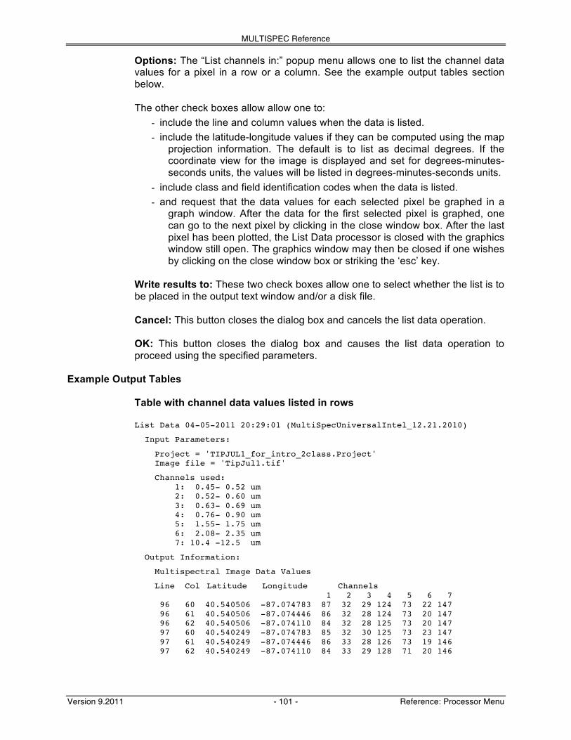
MULTISPEC Reference


Options: The “List channels in:” popup menu allows one to list the channel data values for a pixel in a row or a column. See the example output tables section below. The other check boxes allow allow one to:

- include the line and column values when the data is listed. - include the latitude-longitude values if they can be computed using the map

projection information. The default is to list as decimal degrees. If the coordinate view for the image is displayed and set for degrees-minutes-seconds units, the values will be listed in degrees-minutes-seconds units.

- include class and field identification codes when the data is listed. - and request that the data values for each selected pixel be graphed in a

graph window. After the data for the first selected pixel is graphed, one can go to the next pixel by clicking in the close window box. After the last pixel has been plotted, the List Data processor is closed with the graphics window still open. The graphics window may then be closed if one wishes by clicking on the close window box or striking the ‘esc’ key.

Write results to: These two check boxes allow one to select whether the list is to be placed in the output text window and/or a disk file. Cancel: This button closes the dialog box and cancels the list data operation. OK: This button closes the dialog box and causes the list data operation to proceed using the specified parameters.

Example Output Tables Table with channel data values listed in rows List Data 04-05-2011 20:29:01 (MultiSpecUniversalIntel_12.21.2010)

Input Parameters:

Project = 'TIPJUL1_for_intro_2class.Project' Image file = 'TipJul1.tif'

Channels used: 1: 0.45- 0.52 um 2: 0.52- 0.60 um 3: 0.63- 0.69 um 4: 0.76- 0.90 um 5: 1.55- 1.75 um 6: 2.08- 2.35 um 7: 10.4 -12.5 um

Output Information:

Multispectral Image Data Values

Line Col Latitude Longitude Channels 1 2 3 4 5 6 7 96 60 40.540506 -87.074783 87 32 29 124 73 22 147 96 61 40.540506 -87.074446 86 32 28 124 73 20 147 96 62 40.540506 -87.074110 84 32 28 125 73 20 147 97 60 40.540249 -87.074783 85 32 30 125 73 23 147 97 61 40.540249 -87.074446 86 33 28 126 73 19 146 97 62 40.540249 -87.074110 84 33 29 128 71 20 146

MULTISPEC Reference


Table with channel data values listed in columns Line Chan Columns 60 61 62 96 1 87 86 84 2 32 32 32 3 29 28 28 4 124 124 125 5 73 73 73 6 22 20 20 7 147 147 147 97 1 85 86 84 2 32 33 33 3 30 28 29 4 125 126 128 5 73 73 71 6 23 19 20 7 147 146 146

MULTISPEC Reference


Processor-> Reformat Submenu Upon mousing down on the Reformat selection, the submenu at right appears. Items in the submenu may be selected by dragging over to the desired selection. The items in this submenu allow one to make changes in the disk file associated with the active image file. “Processor->Reformat->Change/Write Header...” Menu Item The purpose of this menu item is to insert or change the header in the image file associated with the active image window. A header record includes the number of lines, columns, channels, bits per data value, start line and start column in the image file so that one does not need to enter this information each time the image file is opened. The header record may also contain map information about the image file. If the image file contains an ERDAS *.LAN header, then, 'Change Header' will be the name of this menu item. If the image file does not contain a header, then 'Write Header' will be the name of this menu item. If the image file contains a header that MultiSpec recognizes but is not ERDAS *.LAN, then, 'Change Header' will be the name of this radio button but it will not be enabled. This menu item can also be used to update the map information in the header. Upon selecting this menu item, the dialog box below is presented. The Set Header Specifications Dialog Box

MULTISPEC Reference


Header: The popup box allows one to choose the header to be added or changed in the file. There is one choice – ERDAS74. Current Header Parameters: These text information items indicate what the current settings are for the number of lines, columns, channels, data bits, start line and start column. Edit Image Parameters…: This button will cause the "Set Image File Format Specifications” dialog box, described under the Edit-Image Description... menu item, to be displayed to allow one to change the settings. Edit Image Map Parameters…: This button will cause the “Set Map Coordinate Specifications” dialog box, described under the Edit-Image Map Parameter... menu item, to be displayed to allow one to change the settings. Cancel: This button closes the dialog box and cancels the “change or write header” operation. OK: This button closes the dialog box and executes the “change or write header” operation using the parameters requested in the dialog box. This operation may take awhile if the image file is large.

MULTISPEC Reference


"Processor-> Reformat-> Change Image File Format..." Menu Item The purpose of this menu item is to allow one to create a new image file based on that associated with the active image window with a number of format changes such as a subset of lines, columns, channels, plus many others. Selecting this menu item causes the following dialog box to be presented. The Image File Format Change Options Dialog Box

Input file: This text information displays the name of the image file associated with the active image window. Also the number of lines, columns, channels, data bytes, data bits in this image file along with the band format are displayed. This information is available as reference information. Output file: This popup allows one to select 'New file', 'Append to', or 'Modify part' as the operation to be carried out. If ‘Append to’ or ‘Modify part’ is selected one will later have the chance to specify a line or channel number after which to start making changes in an already existing file. See information under the ‘OK’ button description. Transform Data…: This check box causes the “Set Reformat Transform Parameters” dialog box to be presented. It is described below. Data value type: This popup menu allows one to specify the output data value type including number of bits per data value, signed or unsigned, integer or real.

Band format: This popup menu allows one to specify the band interleave format for the output image file. Channels: This popup menu allows one to select a subset of the channels to be used. See ‘Select Channels’ under the Shared Dialog Boxes section.

MULTISPEC Reference


Options: Invert bottom to top: This check box allows one to invert the lines top to bottom relative those in the input file. Invert right to left: This check box allows one to invert the columns left to right relative those in the input file. Swap bytes: This check box allows one to specify that the bytes for two byte data be swapped relative to those in the input file. This option is only available for output files with two byte data values. Write channel descriptions: This check box allows one to specify that the channel descriptions be included in the output image file. This option is only available if the channel descriptions are included in the input image file. Header: This popup menu, shown to the right, allows one to control the type of header to be written. If the output data is in BIL format, one can write an ERDAS header record or a Matlab26 header to the new file. If the Matlab format is selected then the selected output image is written in Matlab file format. The file can be read directly by Matlab. MultiSpec will not be able to read this file. One can also write a GAIA header to this image file if a thematic image is the active image window and a project file is opened. The GAIA header requires statistics from the project file.

Cancel: This button closes the dialog box and cancels the “Change Image File Format” operation. OK: This button closes the dialog box and executes the “Change Image File Format” operation using the specifications requested in the dialog box. For ‘New file’ request: A dialog box will be presented to allow one to give a name to the new output image file and set the location in which to save the file. For ‘Append to’ or ‘Modify part’ request: A dialog box will be present to allow one to selected the image file that one is to append to or modify a part of. After this the dialog box to the right will be presented to allow one to specify the line number (for BIL and BIS image files) or the channel number (for BSQ image files) after which to append the new image file or to modify a part of the selected file, respectively.

26 Matlab is a numeric computation and visualization software system by The Math Works, Inc., 24 Prime Park

Way, Natick, MA 01760-1520.

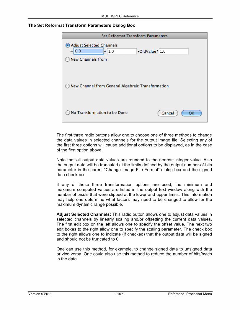
MULTISPEC Reference


The Set Reformat Transform Parameters Dialog Box

The first three radio buttons allow one to choose one of three methods to change the data values in selected channels for the output image file. Selecting any of the first three options will cause additional options to be displayed, as in the case of the first option above. Note that all output data values are rounded to the nearest integer value. Also the output data will be truncated at the limits defined by the output number-of-bits parameter in the parent “Change Image File Format” dialog box and the signed data checkbox. If any of these three transformation options are used, the minimum and maximum computed values are listed in the output text window along with the number of pixels that were clipped at the lower and upper limits. This information may help one determine what factors may need to be changed to allow for the maximum dynamic range possible. Adjust Selected Channels: This radio button allows one to adjust data values in selected channels by linearly scaling and/or offsetting the current data values. The first edit box on the left allows one to specify the offset value. The next two edit boxes to the right allow one to specify the scaling parameter. The check box to the right allows one to indicate (if checked) that the output data will be signed and should not be truncated to 0. One can use this method, for example, to change signed data to unsigned data or vice versa. One could also use this method to reduce the number of bits/bytes in the data.

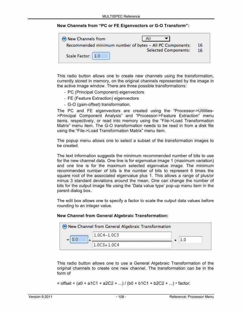
MULTISPEC Reference


New Channels from “PC or FE Eigenvectors or G-O Transform”:

This radio button allows one to create new channels using the transformation, currently stored in memory, on the original channels represented by the image in the active image window. There are three possible transformations:

- PC (Principal Component) eigenvectors - FE (Feature Extraction) eigenvectors - G-O (gain-offset) transformation.

The PC and FE eigenvectors are created using the “Processor->Utilities->Principal Component Analysis” and “Processor->Feature Extraction” menu items, respectively, or read into memory using the “File->Load Transformation Matrix” menu item. The G-O transformation needs to be read in from a disk file using the “File->Load Transformation Matrix” menu item. The popup menu allows one to select a subset of the transformation images to be created. The text information suggests the minimum recommended number of bits to use for the new channel data. One line is for eigenvalue image 1 (maximum variation) and one line is for the maximum selected eigenvalue image. The minimum recommended number of bits is the number of bits to represent 6 times the square root of the associated eigenvalue plus 1. This allows a range of plus/or minus 3 standard deviations around the mean. One can change the number of bits for the output image file using the ‘Data value type’ pop-up menu item in the parent dialog box. The edit box allows one to specify a factor to scale the output data values before rounding to an integer value. New Channel from General Algebraic Transformation:

This radio button allows one to use a General Algebraic Transformation of the original channels to create one new channel. The transformation can be in the form of = offset + (a0 + a1C1 + a2C2 + ...) / (b0 + b1C1 + b2C2 + ...) * factor;

MULTISPEC Reference


where offset, factor, a0, a1, b0, b1, ... are real constants which can be positive or negative and C1, C2, ...Cn represent the channel number to be used27. Both 'c' or 'C' can be used. The number of constant*Channel value (e.g. a1C1) combinations in either the numerator or the denominator is limited to the number of channels in the active image file plus 1. Also the number of characters in the numerator and denominator is limited to 255. Note that this option currently only allows one to create one new channel at a time. A variation for the form of the transformation can be: = offset + (a0 + a1C1*C2 + a2C3 + ...) / (b0 + b1C1*C2 + b2C3 + ...) * factor; In other words, one can multiply the data from two channels. This allows one to do Brovey transforms. Note though that even though one can mix -, +, and * operators, they will be handled strictly left to right. No Transformation to be Done: This radio button allows one to specify that no transformation is to be used. Cancel: This button closes the dialog; no changes are made in the transformation parameter settings. OK: This button closes the dialog box and sets the transformation parameters to those requested in the dialog box.

27 With MultiSpec, one can copy text from another application and then paste it into any dialog edit field. This may

be a convenient method to use here if the General Algebraic Transformation equation is long.

MULTISPEC Reference


"Processor-> Reformat-> Convert Multispectral Image to Thematic Image..." Menu Item (Macintosh OS9 and earlier versions only) The purpose of this menu item is to convert the active multispectral image window to a thematic type of image. This processor uses tools which are available within the Macintosh operating system to determine the 'best' palette of 'n' colors to represent all the colors available in the active multispectral image. This capability is only available when MultiSpec is run under Mac OS (operating system) 7.0 or later. This could be used as a quick way to 'cluster' a multispectral image into a user selected number of classes using the three displayed channels of data. Note that this processor will only use up to 3 channels of data for clustering. If an image has many more than 3 channels then, this technique would not be a good one. Upon selecting this option, the following dialog box will be presented. The Set Multispectral to Thematic Specifications Dialog Box

Color sampling method: These radio buttons allow one to select a method to use to obtain the best set of N colors (defined by the number of classes) to represent the multispectral three channel true or false color image with perhaps thousands or millions of different colors. Number of classes: This edit box allows one to specify how many colors are to be in the output thematic image. Output format: This popup menu allows one to select the header to be included in the new image file. List color table in text window: This check box allows one to choose to list the 8-bit red-green-blue values for each color in the output text window. Cancel: This button closes the dialog box and cancels the “convert multispectral image to thematic image” operation. OK: This button closes the dialog box and executes the “convert multispectral image to thematic image” operation.

MULTISPEC Reference


"Processor-> Reformat-> Convert Project Fields to Thematic Image File..." Menu Item The purpose of this menu item is to create a thematic image showing the training and test fields. Pixels outside of the training or test fields will be represented by the background class. This menu item is useful to create an image file from selected training/test rectangles and polygons that can be used as a mask image file. Upon this option’s selection, the dialog box below is presented. The Project Areas to Thematic Image Dialog Box

Thematic image area: The line and column edit boxes allow one to select the area to be represented in the new thematic image file relative to the training and/or test fields. The button to the left of Line and Column allows one to easily switch between the user selected area (if one has been made in the project image window) and the entire image area. Use: These check boxes allow one to include the training and/or test fields in the output thematic image file. ERDAS header record and trailer file: This check box allows one to specify that an ERDAS *.GIS header should be included in the output thematic image file and a .TRL file should be created that will contain the names of the classes represented in the new thematic image file. Cancel: This button closes the dialog box and cancels the “convert project fields to thematic image file” operation. OK: This button closes the dialog box and executes the “convert project fields to thematic image file” operation using the parameters requested in the dialog box.

MULTISPEC Reference


"Processor-> Reformat-> Convert Shape File to Thematic Image File..." Menu Item The purpose of this menu item is to create a thematic image file that contains class 1 for those pixels that are under a shape file point and 0 for all other pixels that do not include a shape file point. This capability may be expanded in the future.

MULTISPEC Reference


"Processor-> Reformat-> Modify Channel Descriptions..." Menu Item The purpose of this menu item is to add a description of up to 16 characters for each channel in the image file. This is useful in annotating the wavelength range for each channel. One can add, change or delete the descriptions. Upon selecting this menu item, the following dialog box will be presented. The Channel Descriptions Dialog Box

Modify Channel Information for Channel: Selecting this radio button will cause the input channel information to be stored at the end of the multispectral image file when OK is selected. Next channel & Prev channel: These buttons allow one to change the channel that is to be edited. Description: This edit box allows one to enter a description for the channel, e.g. the wavelength limits of the band. The limit is 16 characters. Value: This edit box allows one to enter a value for the channel, e.g. the band number or the center wavelength. Delete Channel Information at end of file: Selecting this radio button will cause all of the channel information stored at the end of the multispectral image file to be deleted when OK is selected. Cancel: This button closes the dialog box and cancels the “modify channel descriptions” operation. OK: This button closes the dialog box and causes the revised channel descriptions to be written to the end of the image file if the Modify radio button is selected or the channel information to be deleted if the Delete radio button is selected.

MULTISPEC Reference


"Processor-> Reformat-> Mosaic Images..." Menu Item (Macintosh Version Only) The purpose of this menu item is to 'mosaic' or join two selected images side to side. Upon its selection, the dialog box below is presented. The Set Mosaic Images Specifications Dialog Box

Left: This text information defines the name of the active image window that will be the basis for the left portion of the new image file. The edit boxes below the text information allow one to select the portion (lines and columns) of the left image to be used. Right: This popup menu allows one to select the image window that is to be used as the basis for the right portion of the new image file. Note that this is a list of the open image windows within MultiSpec not the available data files on disk. The edit boxes below the popup menu allow one to select the start line and the columns of the right image to be used. The end line will be forced to a value such that the number of selected lines in the left image is equal to the number of lines in the right image. Options:

Ignore background value: This check box and edit box allow one to elect to ignore background values when combining the images. This allows one to combine different TM quads. The default background value is 0; the user can set a different background value if needed. Write channel descriptions: This check box allows one to choose to include the channel description information in the new image file. Header: This popup menu allows one to select the header to be included in the new image file.

Cancel: This button closes the dialog box and cancels the “mosaic image” operation.

MULTISPEC Reference


OK: This button closes the dialog box and executes the “mosaic image” operation using the parameters requested in the dialog box. Some Other Notes: Any combination of band interleave for BSQ and BIL may be combined; the output file will have a band interleave of BIL. If either the left or right image has a band interleave of BIS, then both must have a band interleave of BIS. The output band interleave format in this case will be BIS. The number of channels in the left and right images must be the same and the data type in the left and right images must be the same. Only those images that fit the above limitations are enabled in the right image list in the Mosaic Dialog box. The left image defines what format specifications are allowed for the right image.

MULTISPEC Reference


"Processor-> Reformat-> Recode Thematic Image..." Menu Item The purpose of this menu item is to allow one to change the data values in the thematic image file associated with the active image window. This may be helpful in creating or modifying training and test image mask files. Upon selecting this menu item, the following dialog box will be presented. The Set Thematic Recode Parameters Dialog Box

Set data to: This edit box allows one to set the new value that the data are to be changed to when the conditions that follow are met. The name in the quotes is the name of the thematic image file that will be changed. When data value: This popup menu and edit box allow one to set the conditions when data values in the thematic image file are to be changed. The popup menu choices are:

- <= - >= - = - ~= (not equal)

in file: This popup menu to the right allows one to select the file to use to check the conditions on. The default file is the one that is going to be changed. However, one can specify a different file if one wishes. This is a useful approach if one needs to keep the original file for backup purposes.

MULTISPEC Reference


"Processor-> Reformat-> Rectify Image..." Menu Item

The purpose of this menu item is to rectify (change the geometry) of the input selected image. Upon its selection, the dialog box below is presented. One can create a new image in which one or more selected channels are translated and/or rotated with respect to the other channels. Or one can re-project the input image based on the map projection and scale of another reference image which is opened within Multispec, i.e. there is a image window representing the reference image.. The Set Image Rectification Parameters Dialog Box

Input Image Settings: The line and column edit boxes allow one to select the portion of the image to be rectified. The button to the left of Line and Column allows one to easily switch between the user selected area (if one has been made in the project image window) and the entire image area. Output Image Options:

Header: This popup menu allows one to select the header format to be used in the output image file. Set Nonselected Pixels to Background Value: This check box allows one to choose to set non-selected pixels to the background value instead of the value that they currently are. Background value: This edit box allows one to set the data value to use to represent background values. Channels: This popup menu allows one to select a subset of the channels to be shifted, re-scaled and/or rotated. See ‘Select Channels’ under the Shared Dialog Boxes section.

MULTISPEC Reference


Rectification Settings: Offset/Scale: These edit boxes allow one to set the line/column offsets to use to shift the selected channels relative to the non-selected channels. Negative values shift the selected channels by the specified offset value up (lines) or to the left (columns). Positive offset values shift the selected channels by the specified offset value down (lines) or to the right (columns). Scale: These edit boxes allow one to set the line/column scale values to use to re-scale the image. A value of 1.0 indicates no re-scaling. A scale value greater than 1 will cause the new image to be larger. A scale value less than one will cause the new image to be smaller. Rotation (clockwise) Degrees: This edit box allows one to specify the number of degrees to rotate the selected channels. Positive values reflect a clockwise direction; negative values reflect a counter clockwise direction.

Reproject:

Reference: This popup menu allows one to select the image that is to be the reference image for the re-projection. Note that the map projection needs to be known for both the target and reference image files. This re-projection process is done by nearest neighbor re-sampling of the target image so that it matches the extent and map projection of the reference image. First be sure that both the target and reference images are both open with image windows. Make sure that the image that you want to re-project (the target image) is the active image before selecting the Processor-> Reformat-> Rectify Image processor. When one selects the "Reproject" radio button, a popup menu will be displayed which allows you to select the image that you want to reproject the input image to. A new image file will be created using the area of the "reference" image that has been populated with the pixels of the input image file. This is done by determining the latitude-longitude of the center of each pixel in the output image and finding the "nearest neighbor" latitude-longitude pixel in the input image. Note that this will only work if the map projections represent those that MultiSpec currently can handle: Geographic (degrees), Albers Conical Equal Area, Cylindrical Equal Area, Equirectangular, Krovak, Lambert Azimuthal Equal Area, Orthographic, Sinusoidal, State Plane (if for Indiana), Transverse Mercator and UTM. Be aware that no adjustments are made for datum shifts. This feature can be used to create a Landsat thermal band file which as the same spatial pixel size as the reflective bands so that one can include the thermal band with the reflective bands.

Cancel: This button closes the dialog and cancels the “rectify image” operation. OK: This button closes the dialog box and executes the “rectify image” operation using the parameters requested in the dialog box. One will be prompted for a file name for the new output image file. Note that nearest neighbor interpolation is used for the output image file.

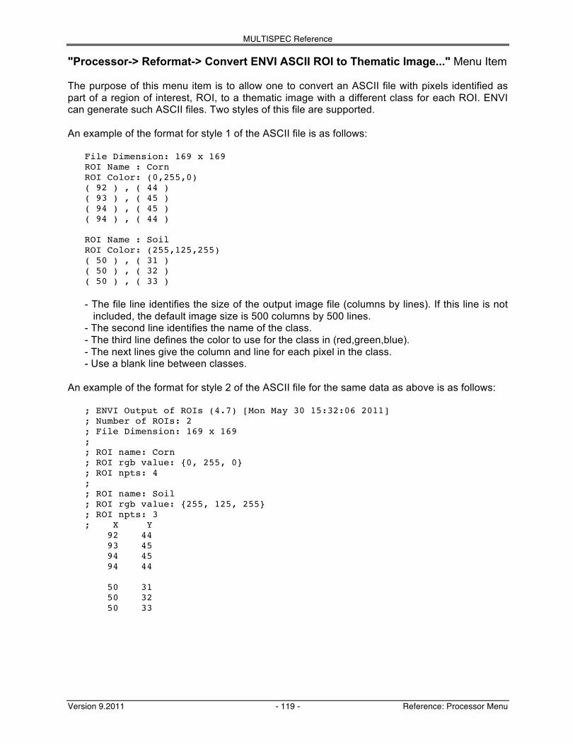
MULTISPEC Reference


"Processor-> Reformat-> Convert ENVI ASCII ROI to Thematic Image..." Menu Item The purpose of this menu item is to allow one to convert an ASCII file with pixels identified as part of a region of interest, ROI, to a thematic image with a different class for each ROI. ENVI can generate such ASCII files. Two styles of this file are supported. An example of the format for style 1 of the ASCII file is as follows:

File Dimension: 169 x 169 ROI Name : Corn ROI Color: (0,255,0) ( 92 ) , ( 44 ) ( 93 ) , ( 45 ) ( 94 ) , ( 45 ) ( 94 ) , ( 44 )

ROI Name : Soil ROI Color: (255,125,255) ( 50 ) , ( 31 ) ( 50 ) , ( 32 ) ( 50 ) , ( 33 )

- The file line identifies the size of the output image file (columns by lines). If this line is not

included, the default image size is 500 columns by 500 lines. - The second line identifies the name of the class. - The third line defines the color to use for the class in (red,green,blue). - The next lines give the column and line for each pixel in the class. - Use a blank line between classes.

An example of the format for style 2 of the ASCII file for the same data as above is as follows:

; ENVI Output of ROIs (4.7) [Mon May 30 15:32:06 2011] ; Number of ROIs: 2 ; File Dimension: 169 x 169 ; ; ROI name: Corn ; ROI rgb value: {0, 255, 0} ; ROI npts: 4 ; ; ROI name: Soil ; ROI rgb value: {255, 125, 255} ; ROI npts: 3 ; X Y 92 44 93 45 94 45 94 44 50 31 50 32 50 33

MULTISPEC Reference


The procedure to convert the file is to: - open the multispectral image file on which the ROI's are based - Select the Processor->Reformat->Convert ENVI ASCII ROI to Thematic Image option - MultiSpec will allow one to select the ROI ASCII file to be used - MultiSpec will then request a name for the output file - The operation is then executed

MULTISPEC Reference


“Processor-> Cluster…” Menu Item This menu item allows one to run one of two clustering algorithms28, a simple one-pass cluster algorithm or an Isodata type iterative algorithm, on the selected image data. Selection of this menu item results in the dialog box shown below. The Set Cluster Specifications Dialog Box

Algorithm: These radio buttons allow one to select the algorithm to be used. Selecting either of these buttons will cause another dialog box to be displayed so that the user can specify the parameters for the selected cluster algorithm. Those dialog boxes are described below. Cluster Classification Map Area(s): These radio buttons allow one to use the calculated cluster statistics to classify training areas or a selected area with a minimum Euclidean distance classifier. Each pixel in the selected classification area(s) is compared to the final cluster centers using the Euclidean distance. The pixel is assigned to the nearest cluster unless it is too far away. A pixel is determined to be too far away if the Euclidean distance squared is more than "number of channels * ‘Classification threshold’ squared". If the pixel is too far away, the pixel is labeled with the blank symbol. If the cluster classification has been requested and the cluster classification map is saved to a disk file, the classification map can be displayed using the “File-> Open Image…” menu item discussed above.

28 See John A Richards, Remote Sensing Digital Image Analysis, First Edition, Springer-Verlag, 1986, pages 197-

199, or Second Editon,1993, pages 236-7.

MULTISPEC Reference


Line/Column: The line and column edit boxes allow one to select the area for which the cluster classification map is to be generated for. The button to the left of Line and Column allows one to easily switch between the user selected area (if one has been made in the image window) and the entire image area.

Classification threshold: This edit box allows one to enter the threshold value to be used in generating the cluster classification map described above. Channels: This popup menu allows one to choose the channels to be used for the clustering operation. The default is all channels. See ‘Select Channels’ under the Shared Dialog Boxes section. Symbols: This popup menu allows one to choose the symbols to be used to represent the cluster classes. See ‘Change Class Symbols’ under the Shared Dialog Boxes section. Cluster Stats: This popup menu allows one to specify how the cluster statistics are to be handled upon completion of the clustering operation. The choices are:

- Do not save the statistics - Save the statistics to a new project file (the

default) If one saves the statistics to a new project file and a project file is already open, then the current project will be closed. The user is given a chance to save the current project if it has changed since the last save. If the cluster statistics are being saved to a new project, the channels for the saved cluster statistics will be those used for the clustering. Note that if one desires to cluster with a subset of channels and save the statistics for all the channels in a new project, then a new project should be created, using the 'New Project' Project menu item before selecting the 'Cluster' processor. Then in the cluster processor select Add to Project'.

- Or add the statistics to those in the current project If one saves the cluster statistics to the current project, the channels used will match those being used in the current project. In other words one can cluster with a different set of channels than one saves the statistics for.

Write cluster report/map to: These check boxes allow one to:

- Write the cluster report and cluster classification map the output text window and/or a disk file.

- Create a cluster mask which identifies the pixels used to generate the

statistics for each of the final cluster classes. The mask file is the same size as the input image that was used for clustering. A value of '1' is used to identify those pixels used for cluster 1, a '2' is used for cluster 2, etc. '0' is used for all pixels that were not used to generate the cluster

MULTISPEC Reference


statistics. The mask file can be treated as a thematic image file and it can be used to define training areas using an option described under the “Processor->Statistics…” menu item.

- Create an overlay of the cluster map on the multispectral image window.

This overlay is created in real time as the cluster operation is being done. One can watch the cluster assignments for the pixels change from pass to pass.

The popup menu allows one to request that a new overlay be created or that a previous overlay be written over.

Cancel: This button closes the dialog box and cancels the cluster operation. OK: This button closes the dialog box and executes the cluster operation using the parameters set in the dialog box.

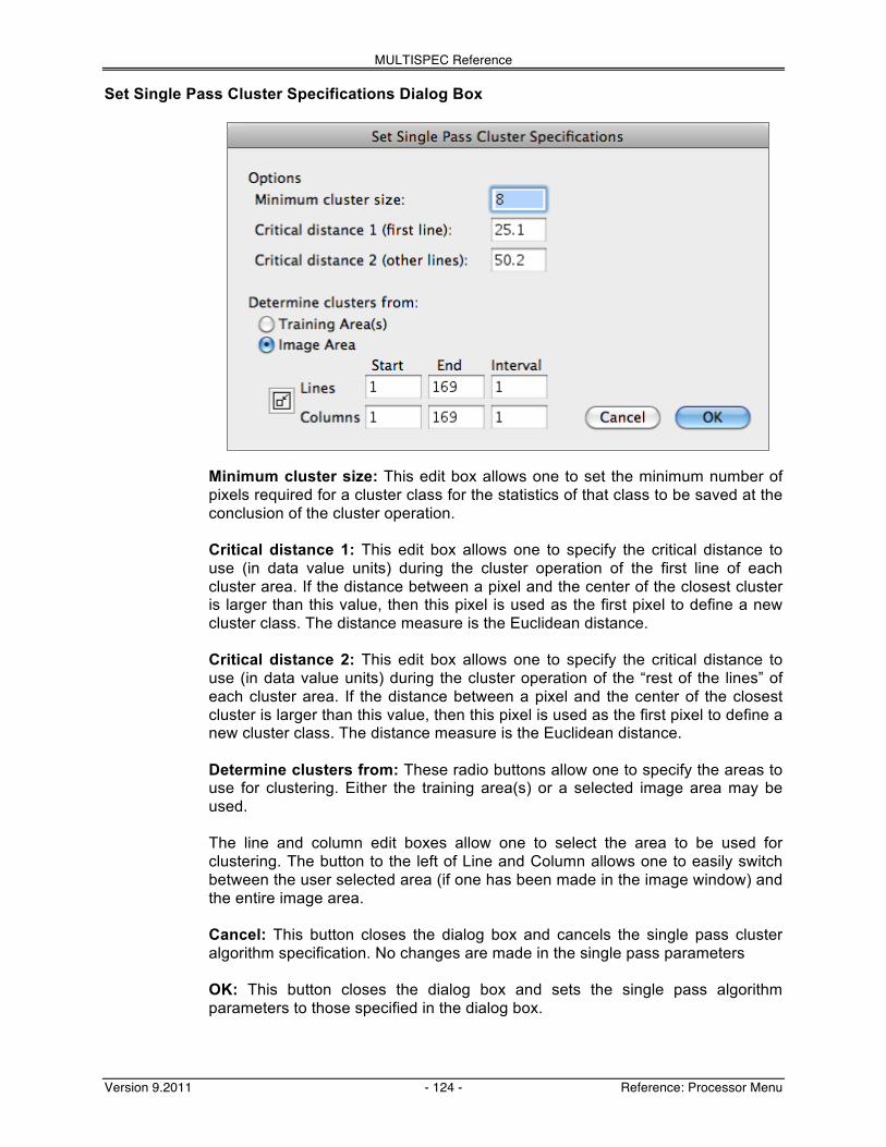
MULTISPEC Reference


Set Single Pass Cluster Specifications Dialog Box

Minimum cluster size: This edit box allows one to set the minimum number of pixels required for a cluster class for the statistics of that class to be saved at the conclusion of the cluster operation. Critical distance 1: This edit box allows one to specify the critical distance to use (in data value units) during the cluster operation of the first line of each cluster area. If the distance between a pixel and the center of the closest cluster is larger than this value, then this pixel is used as the first pixel to define a new cluster class. The distance measure is the Euclidean distance. Critical distance 2: This edit box allows one to specify the critical distance to use (in data value units) during the cluster operation of the “rest of the lines” of each cluster area. If the distance between a pixel and the center of the closest cluster is larger than this value, then this pixel is used as the first pixel to define a new cluster class. The distance measure is the Euclidean distance. Determine clusters from: These radio buttons allow one to specify the areas to use for clustering. Either the training area(s) or a selected image area may be used. The line and column edit boxes allow one to select the area to be used for clustering. The button to the left of Line and Column allows one to easily switch between the user selected area (if one has been made in the image window) and the entire image area. Cancel: This button closes the dialog box and cancels the single pass cluster algorithm specification. No changes are made in the single pass parameters OK: This button closes the dialog box and sets the single pass algorithm parameters to those specified in the dialog box.

MULTISPEC Reference


Description of Single Pass Algorithm The first sample in the first row of the first cluster area defines the center of the first cluster. For each remaining pixel, the closest cluster is found using a standard Euclidean distance measure. Next the data value for each selected channel for the pixel is compared against the closest cluster center value for that channel. If the data value for any channel is more than "critical distance1" units away, then that sample is used as the center of a new cluster. Once all the samples in the first row of all the cluster area(s) have been evaluated, a user specified subset of the remaining samples in the cluster area(s) are used to add to the current clusters or to create new clusters. The pixels are compared to the current clusters as described above for the first line. The only difference is that "critical distance2" is used to determine when to start a new cluster. During the clustering of the "rest of the lines", the user specified column and line intervals are used. Note that the column interval as implemented continues from the end of one line to the beginning of the next selected line. In other words, if the last sample used for clustering in a line of 169 pixels is 166 using a column interval of 5, then the first sample to be used from the next line will be pixel 2. This allows a user the opportunity to use samples from all columns even when a subset is being used. After all the selected area(s) have been clustered, those clusters with fewer pixels than "minimum cluster size" are deleted. Cluster classification then proceeds as described above, assuming that option was selected.

MULTISPEC Reference


Set ISODATA Cluster Specifications Dialog Box

Initializing Options: These radio buttons (and one check box button) allow one to designate how the initialize cluster centers are to be located. The choices are:

- Along first eigenvector, - Within eigenvector volume, - Use one-pass cluster centers.

The “include project class means” checkbox allows one to specify that the current project class means be used as cluster centers along the first eigenvector or within the eigenvector volume. This option is not available for the case for initializing with one pass cluster centers. Determine clusters from: These radio buttons allow one to specify the areas to use for clustering. Either the training area(s) or a selected image area may be used. The line and column edit boxes allow one to select the area to be used for clustering. The button to the left of Line and Column allows one to easily switch between the user selected area (if one has been made in the image window) and the entire image area. Initial number clusters: This edit box allows the user to set the number of initial clusters. Convergence (%): This edit box allows the user to set the percent to use as the threshold to stop the ISODATA iteration. If the number of pixels that do not change cluster classes during one iteration is more than or equal to the convergence percent of the total number of pixels being clustered, then the ISODATA cluster operation is complete.

MULTISPEC Reference


Minimum cluster size: This edit box allows one to set the minimum number of pixels required for a cluster class for the statistics of that class to be saved at the conclusion of the cluster operation. Critical distance 1: This edit box is displayed when the “Use one-pass cluster” initialization options is selected. The edit box allows one to specify the critical distance to use (in data value units) during the cluster of the first line of each cluster area. If the distance between a pixel and the center of the closest cluster is larger than this value, then this pixel is used as the first pixel to create a new cluster. The distance measure is the Euclidean distance. Critical distance 2: This edit box is displayed when the “Use one-pass cluster” initialization options is selected. This edit box allows one to specify the critical distance to use (in data value units) during the cluster of the “rest of the lines” of each cluster area. If the distance between a pixel and the center of the closest cluster is larger than this value, then this pixel is used as the first pixel to create a new cluster. The distance measure is the Euclidean distance. Cancel: This button closes the dialog box and cancels the ISODATA cluster algorithm specification. No changes are made in the ISODATA parameters OK: This button closes the dialog box and sets the ISODATA algorithm parameters to those specified in the dialog box. Note: If one notices diagonal or vertical lines in the clustered data such as the image overlay or the cluster mask file, check the line or column interval used for clustering. The interval needs to be 1 to include all pixels in the cluster operation.

MULTISPEC Reference


Description of ISODATA Algorithm The “along first eigenvector” and “within eigenvector volume” initialization options cause calculation of the principal components of the data. For the “along first eigenvector” initialization option, the specified number of initial cluster centers are equally spaced along the first principal component. For the “within eigenvector volume” initialization option, the initial cluster centers are scattered within the volume defined by the first three principal components. If “include project class means” is requested then the project class means replace those initial centers found above which are nearest to them. For the “use one-pass cluster centers” initialization option, the one-pass clustering algorithm is run first, then the cluster centers determined by it are used as the initial cluster centers for ISODATA clustering. After determining the initial cluster centers, the algorithm proceeds to associate each pixel with the cluster center the smallest Euclidean distance from it; one complete iteration is done after all pixels have been so assigned, and a test for stopping is carried out, as follows. If during that iteration at least P percent of the pixels did not change the cluster center to which they were associated during the previous iteration, the clustering is declared complete. If not, the mean values of all clusters are calculated. These become the new cluster centers, and the clustering process is repeated through another iteration. The clustering stops when the convergence percent has been met. Clustering can also be stopped by entering "Command-.", hold Command key and the period key down at the same time, at the keyboard. If "Command-." is entered, a dialog box will be displayed to allow the user to choose to finish the current pass and save statistics, cancel operation and do not save any statistics, or continue clustering. After clustering has stopped, each cluster is examined to determine if it contains at least the requested minimum number of pixels. If it does not, then that cluster center is not listed and/or saved in the project statistics. Classification then proceeds as described above, assuming that option was selected.

MULTISPEC Reference


“Processor-> Statistics…” Menu Item This menu item allows one to define training and testing areas and to associate them with classes. If the "Statistics" menu item is selected and no project is active, a new project will be activated automatically. (If one wishes to work with a previous project that was created and saved, then use the "File->Open Project" menu item to select the desired project and load it into memory.) Selecting this menu item will also cause the following dialog box to be presented to allow one to set some project related options. The Set Project Options Dialog Box

Project Changes: This popup menu allows one to clear the project statistics or establish a new project. Channels to Use: This popup menu allows one to select a subset of the available channels to be used to compute the mean and covariance statistics. See ‘Select Channels’ under the Shared Dialog Boxes section. Project Statistics Options...: This button causes another dialog box to be displayed to allow one to control other project statistics options. The "Project Statistics Options" dialog box is discussed below. Training mask file: This popup menu item allows one to select an image file that contains a mask that will be used to define the areas in the project base image to be used for the training statistics. This mask file can be in any image format that MultiSpec recognizes. If the image file is a multispectral type of image file, then the mask currently needs to be the first channel of that file. Each different data value other than 0 in the mask file is treated as a different field and class. After selecting a mask and then clicking the "OK" button in the dialog box, the mask data is read into memory and the mask values are assigned to a project class in numerical mask value order. Unused mask values are skipped. For example, if data exists in the mask file for data values of 1, 2, 4 and

MULTISPEC Reference


6, then the mask value of 1 is assigned to project class 1, mask value 2 is assigned to project class 2, mask value of 4 is assigned to project class 3 and mask value 6 is assigned to project class 4. New classes are generated if there are more mask values than there are project classes. If a thematic type of image file is used as the mask and that image file contains the class names to associate with the data values in the file, then those class names are used as the newly generated project class names. Each mask value is treated as a field and has a name associated with it. The name is MaskFieldn when "n" refers to the mask value in the file or when available "classname_Mn" where "classname" is the mask class name and "n" is the mask value. Because each mask value has a field associated with it, one can copy and paste the mask fields from one class to another if they do not happen to be in the same order as the associated classes in the project file. Note that one can have a combination of training fields defined by rectangular or polygonal selected areas and a mask image file. The current methods to generate a mask image file within MultiSpec are to use the "Create cluster mask file" in the Cluster Processor or the "Reformat->Convert Project Fields to Thematic Image File" menu item. One can also generate masks with other software packages that could then be used as input to MultiSpec. Test mask file: This popup menu item allows one to select an image file that contains a mask that will be used to define the areas in the project base image to be used as test areas. See the discussion under "Training mask file" for more information. Outline Selected Areas

Training fields: This check box controls whether the boundaries of the training fields defined by rectangles or polygons are to be shown in the project image window or each associated project image window. Test fields: This check box controls whether the boundaries of the test fields defined by rectangles or polygons are to be shown in the project image window or each associated project image window. Show class names: This check box controls whether the class names are to be shown with each outlined area in the project image window or each associated project image window. Show field names: This check box controls whether the field names are to be shown with each outlined area in the project image window or each associated project image window. Show train/test label: This check box controls whether the train or test label is to be shown with each outlined area in the project image window or each associated project image window. The label is "n" for training and "t" for test. Color: The color popup menu item allows one to control the color of the text and field borders specified in the above check boxes – either black or white.

MULTISPEC Reference


Cancel: This button closes the dialog box and cancels the Processor - Statistics menu item request. No changes are made in the project statistics settings. OK: This button closes the dialog box and causes the selections in the "Set Project Options" dialog box to be accepted and a "Statistics" window to be displayed if one is not already. See the section on "Project Window" for more information.

The Set Project Statistics Options Dialog Box

This dialog box allows one to control some project statistics options.

Compute statistics for: This pair of radio controls allows one to specify whether the means, standard deviations, and covariances are computed, or only the means and standard deviations. If only means and standard deviations are computed then one does not have access to several processors such as Feature Selection, Statistics Image, and the Maximum Likelihood and ECHO Classifiers. The option was made available for those cases when memory is short and second order statistics are not needed.

MULTISPEC Reference


Keep only class statistics in memory: This checkbox allows the user to specify that the class statistics are to be saved in memory instead of the field statistics. The default is to keep the class statistics in memory. This capability exists so that one could use projects that contained many fields of high dimensionality (more than 50 channels or so) for relatively few classes and therefore save memory. There are some drawbacks to keeping only the class statistics. If one cuts a field from a class then the statistics for the class will need to be computed by rereading from the base image disk file. If one keeps the field statistics then the class statistics can be easily computed by summing the field statistics stored in memory. Also it will not be possible to update the statistics for a class if those statistics are defined by cluster fields and one of the fields is cut. Set-zero-variances to: This check box allows one to use class statistics that have zero variance in algorithms that require the second order statistics. In these cases, one can not invert the covariance matrix. This situation occurs, for example, when one has a border around the area of interest which has a constant value such as '0' and one would like to treat this border as a class. This option allows one to reset any '0' variances to a small, specified value. The default value is 0.01. When this checkbox is selected, an edit box appears to allow one to enter the variance value to be used. Minimum log determinant allowed for valid matrix inversion: This edit box allows one to set the log determinant value below which a matrix inversion is considered to be ill-conditioned. The value is in log units. Therefore -25 refers to 10 to the -25 power. Use common covariance in leave-one-out covariance estimations: This checkbox allows control over what matrices are used when the leave-one-out covariance estimator is used. Cancel: This button closes the dialog. No changes will be made in the project statistics options. OK: This button closes the dialog box and causes the selections in the " Set Project Statistics Options " dialog box to be accepted. The user is returned back to the "Set Project Options" dialog box.

MULTISPEC Reference


“Processor-> Enhance Statistics…” Menu Item This processor computes class statistics in a combined supervised-unsupervised mode by using “non-labeled” samples to modify or enhance the statistics for the labeled samples. This processor is based upon research results of recent origin.29,30,31,32,33,34 The processor is based upon modeling the entire data set by a linear combination of weighted Gaussian density functions. It uses an iterative process to achieve a best fit of this model to the combination of the training samples and the designated unlabeled samples, by sequentially adjusting the class mean vectors, class covariance matrices and the class weights (which in this case become estimates of the a posteriori class probabilities). The adjustment is made using a process known as “expectation maximization.” Provision is made to ignore outlier pixels, i.e., pixels whose likelihood value for any of the classes is below a user-selected threshold. Part III, Using MultiSpec, provides an example of using this processor and illustrates some of the potential benefits this process can provide. Selecting this menu item will display the following dialog box to allow one to set some parameters before execution. The Set Statistics Enhancement Specifications Dialog Box

29 Behzad M. Shahshahani and David A. Landgrebe, "Using Partially Labeled Data For Normal Mixture

Identification With Application To Class Definition," Proceedings of the International Geoscience and Remote Sensing Symposium (IGARSS'92), Houston, TX, pp 1603-5 May 26-29, 1992.

30 B.M. Shahshahani, D.A. Landgrebe, "On the Asymptotic Improvement of Supervised Learning by Utilizing Additional Unlabeled Samples; Normal Mixture Density Case," SPIE Int. Conf. Neural and Stochastic Methods in Image and Signal Processing, San Diego, CA, July 19-24, 1992.

31 Behzad M. Shahshahani and David A. Landgrebe, “Use Of Unlabeled Samples For Mitigating The Hughes Phenomenon” Proceedings of the International Geoscience and Remote Sensing Symposium (IGARSS'93), Tokyo, pp 1535-7, August 1993.

32 Behzad M. Shahshahani and David A. Landgrebe, “Classification of Multi-Spectral Data By Joint Supervised-Unsupervised Learning,” PhD thesis, School of Electrical Engineering, Purdue University, December 1993, School of Electrical Engineering Technical Report TR-EE-94-1, January, 1994.

33 Behzad M. Shahshahani and David A. Landgrebe, “The Effect of Unlabeled Samples in Reducing the Small Sample Size Problem and Mitigating the Hughes Phenomenon,” IEEE Transactions on Geoscience and Remote Sensing, Vol. 32, No. 5, pp 1087-1095, September 1994.

34 Saldju Tadjudin and David A. Landgrebe, “Robust Parameter Estimation for Mixture Model,” IEEE International Geoscience and Remote Sensing Symposium, Seattle, WA July 6-10, 1998.

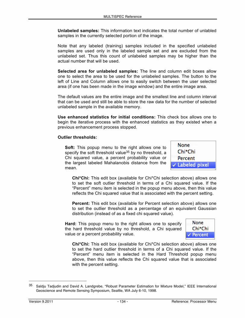
MULTISPEC Reference


Unlabeled samples: This information text indicates the total number of unlabled samples in the currently selected portion of the image. Note that any labeled (training) samples included in the specified unlabeled samples are used only in the labeled sample set and are excluded from the unlabeled set. Thus this count of unlabeled samples may be higher than the actual number that will be used. Selected area for unlabeled samples: The line and column edit boxes allow one to select the area to be used for the unlabeled samples. The button to the left of Line and Column allows one to easily switch between the user selected area (if one has been made in the image window) and the entire image area. The default values are the entire image and the smallest line and column interval that can be used and still be able to store the raw data for the number of selected unlabeled sample in the available memory. Use enhanced statistics for initial conditions: This check box allows one to begin the iterative process with the enhanced statistics as they existed when a previous enhancement process stopped. Outlier thresholds:

Soft: This popup menu to the right allows one to specify the soft threshold value35 by no threshold, a Chi squared value, a percent probability value or the largest labeled Mahalanobis distance from the mean.

Chi*Chi: This edit box (available for Chi*Chi selection above) allows one to set the soft outlier threshold in terms of a Chi squared value. If the “Percent” menu item is selected in the popup menu above, then this value reflects the Chi squared value that is associated with the percent setting. Percent: This edit box (available for Percent selection above) allows one to set the outlier threshold as a percentage of an equivalent Gaussian distribution (instead of as a fixed chi squared value).

Hard: This popup menu to the right allows one to specify the hard threshold value by no threshold, a Chi squared value or a percent probability value.

Chi*Chi: This edit box (available for Chi*Chi selection above) allows one to set the hard outlier threshold in terms of a Chi squared value. If the “Percent” menu item is selected in the Hard Threshold popup menu above, then this value reflects the Chi squared value that is associated with the percent setting.

35 Saldju Tadjudin and David A. Landgrebe, “Robust Parameter Estimation for Mixture Model,” IEEE International

Geoscience and Remote Sensing Symposium, Seattle, WA July 6-10, 1998.

MULTISPEC Reference


Percent: This edit box (available for Percent selection above) allows one to set the outlier threshold as a percentage of an equivalent Gaussian distribution (instead of as a fixed chi squared value).

Labeled samples: Total number of labeled (training) samples in the project file. Classes: This popup menu allows one to choose the classes for which enhanced statistics will be found. The default is all classes. See ‘Select Classes’ under the Shared Dialog Boxes section. Class weights: This popup menu allows one to choose the prior weights for each class. The default is equal weights. See ‘Specify Class Weights’ under the Shared Dialog Boxes section. Weight labeled samples: This allows one to set the weighting of the labeled samples relative to the unlabeled samples (when checked). The default is proportional to the number of samples or a weighting factor of 1.0. Change this factor to 2.0 to double the weighting of the labeled sample or .5 to halve the weight of the labeled samples. Iteration stop conditions: These edit boxes allow one set the stopping conditions. One can set the maximum allowable number of iterations, and the log likelihood change as a percentage over the last N iterations, as set by the Iteration length parameter. One can also stop the iterations before the stopping conditions have been achieved by striking the “Cancel” button in the “Status Dialog Box”. If the operation is stopped, a dialog box will be displayed to allow the user to choose to finish the current iteration (save the current enhanced statistics), don’t finish the current iteration (don’t save the enhancement statistics), or cancel the stop request (continue the statistics enhancement operation). In the Macintosh version only: One can also stop the iterations before the stopping conditions have been achieved by entering "Command-.", hold Command key and the period key down at the same time, at the keyboard. Cancel: This button closes the dialog box and cancels the Statistics Enhancement operation. No changes are made in the settings. OK: This button closes the dialog box and executes the Statistics Enhancement operation using the settings in the dialog box. The outputs of this processor are enhanced class statistics (means and covariances) and prior probabilities. These modified class statistics are stored as a part of the project file and may then be used in the Feature Extraction, Feature Selection, Classify, Principal Components, Create Image Statistics (class statistics only), and Check Covariance processors. The resulting statistics provide a better model to the entire data set to be analyzed, thus improving the generalization from training samples to others and also mitigating the Hughes phenomenon allowing for more effective use of high dimensionality.

Note: One can read a project file containing enhanced statistics written by the Windows version with the Macintosh version. However, one can not read a project file containing enhanced statistics written by the Macintosh version with the Windows version.

MULTISPEC Reference


“Processor-> Feature Extraction…” Menu Item The Feature Extraction processor contains three algorithms, Discrimiant Analysis Feature Extraction (DAFE) and Decision Boundary Feature Extraction (DBFE), and Projection Pursuit. The latter two are recent developments36,37,38,39. DAFE has the advantage of being a short calculation, but it is known not to perform well for classes whose mean vectors are similar. DBFE is a longer calculation, but it does not have the DAFE disadvantage, and it also gives a direct indication of how many features are needed for a given set of classes. Aside from these characteristics, either should perform well in low dimensional situations, however, since DBFE uses the training samples directly, while DAFE uses class statistics estimated from the training samples, they may not do as well as possible in cases of high dimensional data where the training set sizes are limited. For this circumstance a preprocessing algorithm based upon projection pursuit is available for use in making a preliminary reduction in dimensionality, as described in the Using MultiSpec section (pp. 31 ff.). Both DAFE and DBFE calculations proceed by finding an optimal linear transformation of the spectral features. Once determined, this transformation may then be used to form a transformed data set, the features of which are optimally separable and are automatically in order of their importance relative to discriminating between the defined classes. The eigenvalues of the DBFE transformation provide the information as to how many features to use in order to obtain essentially the same accuracy as the full data set would provide. The details of the DBFE algorithm are given in the references cited above. The DAFE algorithm is a more standard discriminant analysis algorithm based on within-class and between-class scatter matrices as follows. Let Σi be the covariance matrix of class i, Pi be the a priori probability of class i, and µi be the mean of class i. Sw = P1*Σ1 + P2*Σ2 + .... is the within class scatter matrix. Sb = P1*(µ1-µ0)*(µ1-µ0)' + P2*(µ2-µ0)*(µ2-µ0)' + ... is between class

scatter matrix and ' denotes transpose. µ0 = P1*µ1 + P2*µ2 + ... Then for DAFE, the transformation is determined by the eigenvalues and eigenvectors of the matrix Sw-1*Sb. There will always be N -1 non-zero eigenvalues where N is the number of classes because rank(Sb ) = rank( Sw-1*Sb ) = N - 1, thus only the first N–1 features derived in this way are reliable. Selecting this menu item will display the following dialog box to allow one to set some parameters before executing. 36 Chulhee Lee and David A. Landgrebe, "Feature Extraction Based On Decision Boundaries," IEEE Transactions

on Pattern Analysis and Machine Intelligence, IEEE Transactions on Pattern Analysis and Machine Intelligence, Vol. 15, No. 4, April 1993, pp 388-400.

37 Chulhee Lee and David A. Landgrebe, “Feature Extraction And Classification Algorithms For High Dimensional Data,” PhD Thesis, Purdue University, December 1992, and School of Electrical Engineering Technical Report TR-EE 93-1, January 1993.

38 Luis Jimenez and David Landgrebe, “Projection Pursuit For High Dimensional Feature Reduction: Parallel And Sequential Approaches,” Presented at the International Geoscience and Remote Sensing Symposium (IGARSS'95), Florence Italy, July 10-14, 1995.


MULTISPEC Reference


The Set Feature Extraction Specifications Dialog Box

Preprocessing Transformation: This popup menu allows one to choose a preprocessing transformation operation including:

- no projection pursuit transformation, - a new projection pursuit transformation, - a previously calculated one.

If one chooses to generate a projection pursuit transform, the “Set Preprocessing Specifications” dialog box is presented, allowing for a number of parameter settings related to it. This dialog box is shown below. Algorithm: This popup menu to the right allows one to select the algorithm to be used for feature extraction. One may select Nonparametric Weighting (NWFE), Decision Boundary (DBFE), Discriminant Analysis (DAFE), or Preprocessing only. Channels: This popup menu allows one to choose to use all or a subset of the channels. See ‘Select Channels’ under the Shared Dialog Boxes section. Classes: This popup menu allows one to choose to use all or a subset of the classes. See ‘Select Classes’ under the Shared Dialog Boxes section. Class Weights: This popup menu allows one to choose to apply equal or unequal weighting to the classes, e.g. the class prior probabilities. See ‘Specify Class Weights’ under the Shared Dialog Boxes section. Interclass Weights: This popup menu allows one to set the weighting for any of the interclass pairs. This feature is useful if one wants to eliminate from

MULTISPEC Reference


consideration subclasses of a given class for which separation is not desired. This option is only available for DBFE. See ‘Specify Class Pair Weights’ under the Shared Dialog Boxes section. List Transformation Matrix: This check box allows one to request that the transformation matrix be listed in the text window. Special Options: This checkbox displays additional options for the Decision Boundary algorithm. An explanation of these special options is contained in the references; they are intended for those who wish to experiment with these additional parameters of the algorithms after having become familiar with the material in the references cited. Ordinarily the default values should produce satisfactory results, and one need not be concerned with the ‘special options.’

Within class threshold: This edit box allows one to set the within class threshold. Interclass threshold: This edit box allows one to set the between class threshold. Min. threshold number: This edit box allows one to set the minimum threshold number. Optimize classes & Percent of all feature accuracy: This checkbox allows one to specify whether optimization (deletion of redundant features) is desired, and if so to what percent of all feature accuracy is desired. Maximum training pixels per class: This edit box allows one to set the maximum number of training pixels per class to use.

Cancel: This button closes the dialog box and cancels the Feature Extraction operation. No changes are made in the settings. OK: This button causes the dialog box to close and the Feature Extraction processor to proceed to calculate the eigenvalues and eigenvectors for the desired linear transformation, stores them in memory, and writes them in the Text Output Window. See the section on the Feature Extraction processor in the “Using MultiSpec” section above for more information for the steps which the DBFE and DAFE algorithms follow. One can then use the transformed features instead of the original ones in the Classify, Feature Selection, Create Statistics Image, or Check Covariances processors by selecting the appropriate check box when beginning the execution of any of these four processors. Alternatively, one can use the Reformat processor to create a new file with these transformed features instead of the original bands. See the ‘Change Image File Format’ of the Reformat processor above. After completing the Reformat operation, one can use the ‘Project-> Change Base Image’ menu item to make the new file the base image, and choose the Classify processor. In the Classify Processor, choose the first N features where N is selected based upon the accumulative proportion of the transformation eigenvalues or by other means and classify.

MULTISPEC Reference


The Set Preprocessing Specifications Dialog Box

An explanation of these parameter settings is contained in the references; they are intended for those who wish to experiment with these additional parameters of the algorithms after having become familiar with the material in the references cited40,41,42. Ordinarily the default values should produce satisfactory results.

40 Luis O. Jimenez and David Landgrebe, “High Dimensional Feature Reduction Via Projection Pursuit,” School of

Electrical & Computer Engineering Technical Report TR-ECE 96-5, April 1996. 41 Luis Jimenez and David Landgrebe, “High Dimensional Feature Reduction Via Projection Pursuit,” Proceedings

of the International Geoscience and Remote Sensing Symposium (IGARSS'94),CD-ROM pp 1473-1479, Pasadena, Calif, August 8-12,1994.


MULTISPEC Reference


“Processor-> Feature Selection…” Menu Item This menu item causes calculations to be performed which assist in determining the best subset of channels or features to be used for a given training set. It can also be used to determine the relative degree of separability of tentatively defined classes during the early stage of the training process. This processor calculates the statistical distance between all class pairs for each of the subsets of channel combinations chosen. The results of the calculations are listed in rank order, tabular form in the Text Output window, where they may be viewed and a selection made. Or, alternatively, they may be copied to a spreadsheet and further sorting and calculation done on them. For example, if one wished to find the best 3 channels out of 7 available, the processor would calculate and add up the statistical distances between all class pairs for each possible 3 channel subset. The table would then show on each line, the distances between all the class pairs for a given subset and the subsets would be listed in the table in sorted order, for example, in order of decreasing average interclass distance. Upon choosing the "Feature Selection" menu item, a dialog window appears as follows. The Set Feature Selection Specifications Dialog Box

Distance measure: This popup menu item allows one to choose the distance measure to be used. The choices are:

- Bhattacharyya - Error-function Bhattacharyya - “Mean” Bhattacharyya - “Covariance” Bhattacharyya - Non-Covariance Bhattacharyya - Transformed Divergence - Divergence

See the “Description of Feature Selection Distance Measures” section below.

MULTISPEC Reference


Use feature transformation: This checkbox specifies whether the feature selection processor is to use the statistics for the original channels (unchecked) or the transformed channels (checked). This option is only available if a transformation matrix is available by running a principal component analysis, a feature extraction analysis or reading a transformation from a disk file that had been previously saved by MultiSpec. Channels/Features: This popup menu allows one to use all or a subset of the available channels (original channels) or features (transformed channels) in the project statistics. See ‘Select Channels’ under the Shared Dialog Boxes section. Channel Combinations: This group of popup menus, check boxes and edit boxes allow one to select how the channels are to be grouped in sets of channel combinations.

Number of channels: This popup menu allows one to choose the number of groups of channels. There is no default for this parameter; it must be set before the feature selection algorithm can be run. See the description of the “Set Number of Channels to Use” dialog box below. Contiguous channels per group: This edit box allows one to request 'n' groups of channels (selected with the “Number of channels” popup menu above) with 'm' contiguous channels in each group. This feature is particularly helpful when one has a large number of channels of data, and spectral classes which, for example, have unique absorption features expressed in ‘m’ contiguous channels. This option can reduce the number of channel combinations to be searched substantially while focusing on diagnostic features that occur across a small number of adjacent channels. The more conventional selection of optimal channel combinations can be used by setting the number of contiguous channels to 1. Use step procedure: This check box allows an alternate procedure to find the best combination that is also intended for the case of large numbers of bands. The step-wise search technique consists of first finding the best single group of m (m≥1) contiguous channels. Then using the best single group, find the best 2 groups of m channels, then the best 3 groups, etc. up to the number of groups of channels specified by the user. This technique is a sub-optimum search since one is not guaranteed of finding the best set of all possible combinations. However, it does allow one to at least examine a reasonable number of the channel combinations in a high dimensional data set. The number of channel combinations to be searched can be reduced considerably in this way. For example the best 4 out of 210 channels includes millions of combinations. Using the step procedure, the number of combinations to be searched is reduced to a few thousand. Note however that the number of combinations to be searched when one is choosing n-1 of n or n of n channels will be higher for the step search than for the exhaustive search technique. Max search combinations: This text information provides the user with a count of the maximum number of combinations that will be searched for the current settings. For example, if there are 12 channels available and

MULTISPEC Reference


contiguous channels per group is one, there are 495 possible combinations of 4 channels out of the 12. Max number combinations to list: This edit box allows the user to set the number of combinations (after ranking) to list in the output text window.

Classes: This popup menu allows one to choose to use all or a subset of the classes. See ‘Select Classes’ under the Shared Dialog Boxes section. Weights: This popup menu allows one to set the weighting for any of the class pairs. This feature is useful if one wants to eliminate from consideration subclasses of a given class for which separation is not desired. See ‘Specify Class Pair Weights’ under the Shared Dialog Boxes section. Symbols: This popup menu allows one to choose the symbols to be used to represent the classes. See ‘Change Class Symbols’ under the Shared Dialog Boxes section. List Options…: Clicking on this button causes the “Set Feature Selection List Options” dialog box to be displayed to allow one to set some list options. The dialog box is described below. Write results to: These two check boxes allow one to select whether the feature selection table is to be placed in the output text window and/or a disk file. Cancel: This button closes the dialog box and cancels the Feature Selection operation. No changes will be made in the Feature Selection parameters. OK: This button closes the dialog box and executes the Feature Selection operation using the requested specifications. NOTES: The columns of numbers in the feature selection tables are separated by tabs so that they can be copied into a spreadsheet program for further analysis. The program will not allow one to run a feature selection analysis of the best m channels out of n total channels if the number of combinations is greater than 2,147,483,647; of course one probably does not want to come close to this number anyway!

MULTISPEC Reference


The Select Number of Channels to Use Dialog Box

List of Possible Numbers: This list allows one to select the number of channels or groups of channels to use. Click on the number to select that number. The selected numbers are highlighted. One can hold the shift or command key down to make multiple selections in the list. Number selected: This information text line indicates how many items are currently selected in the list above. All: This button allows one to select everything in the list to the left. None: This button allows one to clear all of the selections in the list to the left. First, Last, Interval, Enter new range: The edit boxes allow one to select the first and last number of channels or groups of channels in the list to the left plus an interval. The ‘Enter new range’ button allows one to enter the values specified in the edit boxes into the list. The list is updated automatically when one makes changes in the edit boxes. The ‘Enter new range’ button is useful, if one uses the ‘All’ or ‘None’ buttons and then one wants to change the list back to those specified in the edit boxes. Cancel: This button closes the dialog box and cancels the ‘Select Number of Channels’ request. OK: This button closes the dialog box and sets the number of channels or groups of channels to use to that specified in the dialog box. For example, in the list above, by selecting 4, one requests that the best 4 of the 12 available channels be found by the feature selection processor.

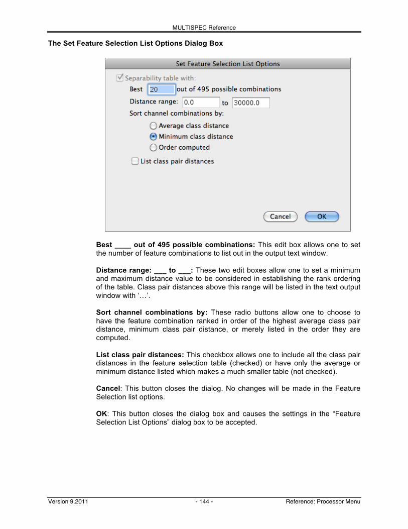
MULTISPEC Reference


The Set Feature Selection List Options Dialog Box

Best ____ out of 495 possible combinations: This edit box allows one to set the number of feature combinations to list out in the output text window. Distance range: ___ to ___: These two edit boxes allow one to set a minimum and maximum distance value to be considered in establishing the rank ordering of the table. Class pair distances above this range will be listed in the text output window with ‘…’. Sort channel combinations by: These radio buttons allow one to choose to have the feature combination ranked in order of the highest average class pair distance, minimum class pair distance, or merely listed in the order they are computed. List class pair distances: This checkbox allows one to include all the class pair distances in the feature selection table (checked) or have only the average or minimum distance listed which makes a much smaller table (not checked). Cancel: This button closes the dialog. No changes will be made in the Feature Selection list options. OK: This button closes the dialog box and causes the settings in the “Feature Selection List Options” dialog box to be accepted.

MULTISPEC Reference


Description of Feature Selection Distance Measures The definition of the Bhattacharyya distance is as follows.

B = µ1 ! µ2[ ]T "1 + "22

# $

% &

!1

µ1 ! µ 2[ ]+12ln

12"1 + "2[ ]|"1||" 2 |

where µx is a mean vector and Σx is a covariance matrix. It may be noted that the first term accounts for the separation due to the class means (normalized with respect to the class covariances), while the second term accounts for the separation due to the class covariances. In the case of the Non-Covariance Bhattacharyya, only the first term is used, and the off-diagonal terms of Σ1 and Σ2 are set to zero. In the case of the Error function Bhattacharyya, the Bhattacharyya distance is mapped through the Gaussian error function, so that the results are more nearly linearly related to probability of error and thus more nearly project what the classification error rate a given value of Bhattacharyya distance implies. Divergence and Transformed Divergence43 are other alternatives that are usually not as effective as those based upon Bhattacharyya distance and are included for historical reasons.

43 See John A Richards, Remote Sensing Digital Image Analysis, First Edition, Springer-Verlag, 1986, pages 207-

214, or Second Editon,1993, pages 246-253 for a detailed discussion of Divergence and Transformed Divergence.

MULTISPEC Reference


“Processor-> Classify…” Menu Item This menu item allows one to classify selected portions of the target image file using the project statistics. Execution of this menu item will cause the following dialog box to be presented. The Classification Specifications Dialog Box

Procedure: This popup menu to the right allows one to choose the classification algorithm to be used. The choices are the Gaussian Maximum Likelihood (Quadratic Likelihood), Fisher Linear Discriminant, Minimum Euclidean Distance, ECHO spectral-spatial, Correlation (spectral angle mapper), and Matched Filter (constrained energy minimization). Selecting the ECHO and Matched Filter classifiers will cause an additional dialog box to be displayed to allow one to set some additional parameters that are unique to them. These dialog boxes are described below. Additionally if one holds the option key (Macintosh version) or right mouse button or shift key (Windows version) down before mousing down on the Procedure popup menu, one can cause another dialog box to be displayed when the Correlation classifier is selected. Again this dialog box is described below. Use feature transformation: This checkbox allows one to specify whether the classify processor is to use the statistics for the original channels (unchecked) or the transformed channels (checked). This option is only available if a transformation matrix is available by running a principal component analysis, a

MULTISPEC Reference


feature extraction analysis or reading a transformation from a disk file that has been previously saved by MultiSpec. Channels/Features: This popup menu allows one to choose to use all or a subset of the available channels (original channels) or features (transformed channels) in the project statistics. See ‘Select Channels’ under the Shared Dialog Boxes section. Target: This text information indicates what the target data set is, i.e. the one to be classified. If there are more than one image data file open with the same number of features and the same data type, this item becomes a pop-up menu allowing one to select which file is to be classified. The file to be classified does not have to be the one that the training statistics came from. Classify: The area in the lower left, under "Class areas:," allows for designation as to what data will be classified, the Training Fields, the Test Fields, and/or a rectangular area of the image file designated by start, end, and intervals. The check boxes labeled Training (resubstitution) and Training (leave-one-out) also control how the results of the classification will be evaluated in these cases. Resubstitution refers to using the proportion of training samples that have been correctly classified. However, it is well known that this method of estimating accuracy is optimistically biased. The leave-one-out method, on the other hand, is unbiased. Test areas previously designated in the Statistics Processor may also be selected, and this method of evaluation is often referred to as the "holdout" method, since labeled samples which might have been used in training are held out to provide a degree of testing as to how well the classifier generalizes from samples used in training to samples not used in training. Classes: This popup menu allows one to choose to use all or a subset of the training classes. See ‘Select Classes’ under the Shared Dialog Boxes section. Class weights: This popup menu allows one to choose to apply equal or unequal weighting to the classes, e.g. the class prior probabilities. See ‘Specify Class Weights’ under the Shared Dialog Boxes section. Symbols: This popup menu allows one to choose the symbols to be used to represent the classes in any alphanumeric classification. See ‘Change Class Symbols’ under the Shared Dialog Boxes section. Write classification results to:

Disk file: This check box allows one to specify whether the classification results are to be written to a disk file. If this option is selected, a popup menu, shown to the right, is made available to allow one to choose one of four output formats. If the map information is available for the output classification from the base image file, the choice will be GeoTIFF instead of TIFF. A .trl file is generated for TIFF/GeoTIFF format so that MultiSpec has access to the class names which are not stored in TIFF/GeoTIFF formatted files.

MULTISPEC Reference


Image window overlay: This check box allows one to request that the classification be overlaid on the multispectral image window. The popup menu below the check box allows one to create a new overlay for the window or replace one that was created before. One can view an image of the classification as it progresses. Palette: If ERDAS.GIS or TIFF/GeoTIFF disk file format is selected, this popup menu is made available. The popup menu, shown to the right, is used to define the colors to be assigned to the classes in the trailer (.TRL) file that is written along with the classified image (.GIS or .TIF) file. The choices here are the same as those described for the Display Image… (Thematic) menu item. Also see the description for the ‘Assign Channels for False Color Palette’ dialog box under the Shared Dialog Boxes section.

The Blue-Green-Red palette, used elsewhere to create Statistics Images, is one with a fairly smooth (subtle) transition from one color to the next, i.e. from one class to the next. When one selects 'False Color...' a dialog box will appear which allows one to select the channels in each class mean vector to define the red, green and blue value for each thematic color. Note that an open project file is required for this option. See the description for the ‘Assign Channels for False Color Palette’ dialog box under the Shared Dialog Boxes section. If written to a disk file, the results may then be displayed as a color coded thematic map by opening an image window in thematic format. Threshold results at ____: For the Maximum Likelihood, Fisher Linear Discriminant and ECHO classifiers, one may also apply a threshold value such that pixels whose largest likelihood value is below the threshold are assigned to a "classification declined" or “thesholded” class. When this checkbox is selected, a edit box will appear allowing the threshold level to be set to a certain percentage value equal to the proportion of an ideal Gaussian distribution which would be thresholded. One may also apply threshold values for the SAM and CEM classifiers. The SAM threshold may be in degrees or a correlation coefficient value. The CEM threshold is a unitless value, usually between 0.5 and 1.0 Create Probability Results File: Create SAM Values File: Create CEM Values File: For the Maximum Likelihood, Fisher Linear Discriminant and ECHO classifiers, this check box allows one to designate that a Probability Results File will be created. In this case, instead of each pixel being assigned to a certain class, the likelihood value of the most likely class is stored for each pixel. This file can then be displayed in color coded thematic form to illustrate the degree of membership

MULTISPEC Reference


of each pixel to its assigned class. The average probability of correct classification is listed in the Text Output window as the classification is completed. For the SAM and CEM classifiers, this check box is named “Create SAM Values File” or “Create CEM Values File”, respectively. In this case the SAM or CEM value is stored for each pixel in a disk file. This file can then be displayed in color coded thematic form. If one has created both a Probability Results (or Values) map and a thematic map (disk file) of the classification results, then one can apply a threshold to the results after the classification has been completed. See the “Processor-> List Results” menu item section. Results List Option...: This button displays another dialog box that allows one to control what is included in the classify processor text output. Cancel: This button closes the dialog box and cancels the Classify operation. No changes will be made in the Classify parameters. OK: This button closes the dialog box and executes the Classify operation using the specifications requested in the dialog box.

The Classification Results List Options Dialog Box

These check boxes allow one to control for both Training and Test data whether the area listings, area classification summaries, area performance summary tables and class performance summary tables are to be listed. This feature is useful for those cases when there are hundreds of areas used for training and/or testing. In this case, the output in the text output window becomes very large.

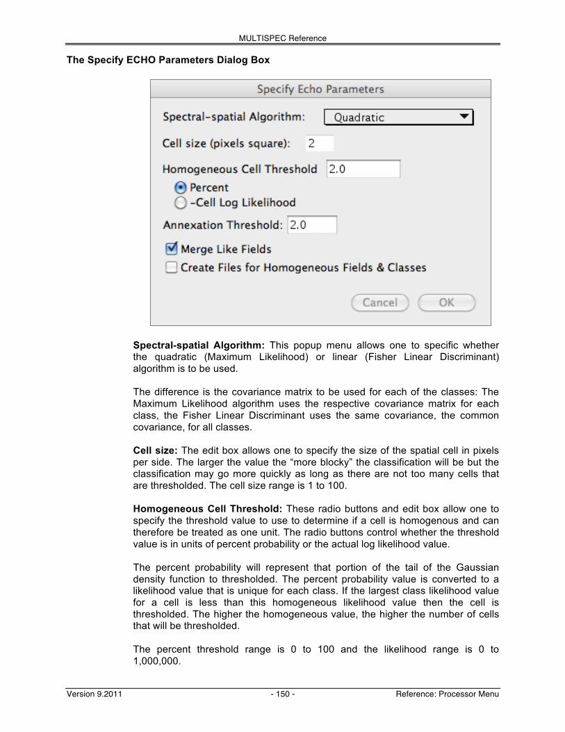
MULTISPEC Reference


The Specify ECHO Parameters Dialog Box

Spectral-spatial Algorithm: This popup menu allows one to specific whether the quadratic (Maximum Likelihood) or linear (Fisher Linear Discriminant) algorithm is to be used. The difference is the covariance matrix to be used for each of the classes: The Maximum Likelihood algorithm uses the respective covariance matrix for each class, the Fisher Linear Discriminant uses the same covariance, the common covariance, for all classes. Cell size: The edit box allows one to specify the size of the spatial cell in pixels per side. The larger the value the “more blocky” the classification will be but the classification may go more quickly as long as there are not too many cells that are thresholded. The cell size range is 1 to 100. Homogeneous Cell Threshold: These radio buttons and edit box allow one to specify the threshold value to use to determine if a cell is homogenous and can therefore be treated as one unit. The radio buttons control whether the threshold value is in units of percent probability or the actual log likelihood value. The percent probability will represent that portion of the tail of the Gaussian density function to thresholded. The percent probability value is converted to a likelihood value that is unique for each class. If the largest class likelihood value for a cell is less than this homogeneous likelihood value then the cell is thresholded. The higher the homogeneous value, the higher the number of cells that will be thresholded. The percent threshold range is 0 to 100 and the likelihood range is 0 to 1,000,000.

MULTISPEC Reference


Annexation Threshold: This edit box allows one to set the threshold value that determines which cells are to be combined into fields. If the annexation value for a cell to a field or a field to a field is less than this value then the two are treated as separate fields. The higher the annexation value, the lower the number of homogeneous fields for a given homogeneous cell threshold. The annexation threshold range is 0 to 100. Merge Like Fields: This check box allows one to control whether to annex (combine) like fields. If this box is not checked then only cells are combined with fields, not fields to fields. Create Files for Homogeneous Fields & Classes: This check box allows one to request additional output disk files showing the boundaries of homogeneous fields and classes to be created (if checked). These additional files can be used to form scene segmentation maps of the data. Cancel: This button closes the dialog. No changes will be made in the ECHO parameters. OK: This button closes the dialog box and causes the ECHO parameters set in the dialog box to be accepted.

Description of the ECHO Classifier ECHO (Extraction and Classification of Homogeneous Objects)44 is a spatial-spectral classifier, i.e. one that incorporates not only spectral variations but spatial ones as well into the decision-making process. It uses a two stage process, first segmenting the scene into statistically homogeneous regions, then classifying the data based upon a maximum likelihood object classification scheme. It uses exactly the same training procedures and statistics as a conventional maximum likelihood pixel classifier, however there are three selectable parameters that the user may set to vary the degree and character of the spatial relationship used in the classification. These parameters enable one to vary the spatial characteristics used from little or none to those incorporating image texture over a block area surrounding each pixel. The segmentation stage of the classifier, itself, is carried out in two stages. In the first stage cells, consisting of contiguous n x n regions (cell size n is set by the user) are checked with a mild test for statistical homogeneity. The threshold used in the test is set by the user. Cells failing this test are said to be singular, and the pixels contained will ultimately be classified by a maximum likelihood pixel classifier. This allows for the proper classification of isolated cells within otherwise homogenous objects. After the cell selection test, next neighboring non-singular cells are compared with a statistical homogeneity test using ratios of the cell log likelihood and field (or region) log likelihoods. Those passing the test

44 R. L. Kettig and D. A. Landgrebe, "Computer Classification of Remotely Sensed Multispectral Image Data by

Extraction and Classification of Homogeneous Objects," IEEE Transactions on Geoscience Electronics, Volume GE-14, No. 1, pp. 19-26, January 1976.

D.A. Landgrebe, "The Development of a Spectral-Spatial Classifier for Earth Observational Data," Pattern

Recognition, Vol. 12, No. 3, pp. 165-175,1980.

MULTISPEC Reference


are “annexed” thus growing regions. The threshold used in this test is, again, set by the user. After all annexation tests are complete, the homogeneous regions thus identified are classified using a maximum likelihood object classification scheme. With a proper choice of parameter values, ECHO usually provides higher accuracy than a pixel classifier and frequently requires less computation time for a given classification task. In addition to the thematic classified result, when instructed to write the results to disk, the ECHO processor may be requested to write files giving the homogeneous fields or objects found (_echoField suffix) and those fields combined into classes (_echoClasses suffix). Thus it can serve as a scene segmenter without classification; however, in order to obtain good results, training statistics for each class occurring in the scene should be provided. Note that cells which do not meet the statistical homogeneity test are thresholded in the _echoField and _echoClasses files. A large number of thresholded pixels in these files indicates that either classes exist which are not represented in the training set, the size of the homogeneous areas are smaller than the cell size, or the homogeneous threshold was set at too stringent of a level. Note that for large image files MultiSpec will write intermediate data that is needed during the echo classify process to a temporary disk file when it can not be stored in the available memory. This temporary file is deleted after the classification has completed. A message is displayed if MultiSpec does not think there is enough disk space available for the temporary file.

The Specify SAM Parameters Dialog Box

Class Covariance: This popup menu allows one to choose whether the covariance matrix is to be used in the correlation classifier (spectral angle mapper). The choices are:

- Do not use - Common covariance - Sample covariance

The use of a covariance matrix in the correlation classifier algorithm ‘normalizes’ the data from channel to channel in the same way that the covariance matrix normalizes the data in the Maximum Likelihood or Fisher Discriminant classifiers. The default is “do not use”.

MULTISPEC Reference


Cancel: This button closes the dialog. No changes will be made in the SAM parameters. OK: This button closes the dialog box and causes the SAM parameters set in the dialog box to be accepted.

Description of the SAM Classifier The Spectral Angle Mapper (SAM)45 is a correlation classifier. This classifier compares the shape of the spectral response of the sample to the mean for each of the training classes using a correlation coefficient ignoring the absolute difference or offset between the spectral response curves. One can set a threshold using the correlation coefficient value or an angle derived from the inverse cosine of the correlation coefficient. This is where the term spectral angle mapper comes from.

The Specify CEM Parameters Dialog Box

Area(s) to use for background correlation matrix: These radio buttons allow one to specify how the backgound correlation marix is to be created. It can be from the combination of selected classes or from a selected area. If “Classes:” is selected, a popup menu will appear to allow one to select a subset of the classes. Cancel: This button closes the dialog. No changes will be made in the CEM parameters. OK: This button closes the dialog box and causes the CEM parameters set in the dialog box to be accepted.

45 Kruse F.A., et. al. 1993. "The Spectral Image Processing System (SIPS) - Interactive Visualization and Analysis of

Imaging Spectrometer Data. Remote Sensing of Environment, v. 44, p. 145-163.

MULTISPEC Reference


Description of the CEM Classifier

A description of the Constrained Energy Minimization (CEM) classifier can be found in Harsanyi (1993)46 and Resmini (1997)47. For the implementation in MultiSpec, the CEM value closest to ‘1’ is considered to be the closest class, not the highest CEM value.

46 Harsanyi, J.C. 1993. Detection and Classification of Subpixel Spectral Signatures in Hyperspectral image

Sequences. PhD Dissertation, University of Maryland, Baltimore County. 47 Resmini, R.G., J.C. Harsanyi, et. al, 1997. “Mineral mapping with Hyperspectral Digital Imagery Collection

Experiment (HYDICE) sensor data at Cuprite, Nevada, U.S.A., Int. J. Remote Sensing, 1997, Vol. 18, No. 7, pp 1553-1570.

MULTISPEC Reference


“Processor-> List Results…” Menu Item This menu item becomes available whenever a thematic image is the active window. It is used to provide tables showing the assignment of pixels in the active window to the classes defined. Upon selection of the List Results menu item, the dialog box shown below is displayed. The List Results Specifications Dialog Box

List results for following areas: These check boxes allow one to select training areas, test areas, and/or a selected image area. To use training areas one must have a project open. To use test areas, one must have a project open which has test areas defined.

The line and column edit boxes allow one to select the area that the results table is to represent. The button to the left of Line and Column allows one to easily switch between the user selected area (if one has been made in the image window) and the entire image area. The default values are the selected area; if none has been selected, then the default is the entire image. Summarize by (train/test only): These check boxes allow one to choose whether Fields, Classes, and/or Groups summary tables are to be listed. This option only applies to training and testing areas. The fields, classes and/or groups will be listed in rows. To obtain a grouping summary, one must have grouped the classes in the thematic image window. See “Combining Classes into Information Groups” under the “Thematic Image Window” section above. Table Type: These radio buttons allow one to specify the table type - class or group. The columns represent the classes or groups in the thematic image file. Table Units: These radio buttons allow one to specify the units for the table - samples, percent of samples, or area. If 'area units' is selected, one may specify an area conversion factor to be used, e.g. hectares per pixel. Threshold Results: This check box and edit box allow one to set the threshold level to use. If one has both the classification file and the probability results (or values) file for the classification open and the classification window is active, one

MULTISPEC Reference


can threshold the results. Selecting this check box will cause an edit box to appear in which the desired threshold level can be set. Write results to: These check boxes allow one to select whether the table(s) will be listed in the Output Text Window and/or a disk file. Cancel: This button closes the dialog box and cancels the List Results operation. No changes will be made in the List Results parameters. OK: This button closes the dialog box and executes the List Results operation using the requested specifications. The width of each column in the results table is controlled by the length of the class or group name. Up to the first 12 characters of the class or group names is used.

Example Output Table

List Results 04-06-2011 13:37:49 (MultiSpecUniversalIntel_12.15.2010)

Input Parameters:

Project = 'flc1.Project' Image file = 'flc1.gis' Project Classes used: Group 1: Alfalfa 3: Ag Crops 2: Bare Soil 2: Bare Soil 3: Corn 3: Ag Crops 4: Oats 3: Ag Crops 5: Red Clover 3: Ag Crops 6: Rye 3: Ag Crops 7: Soybeans 3: Ag Crops 8: Water 4: Water 9: Wheat 3: Ag Crops

Thematic Image Classes Group 0: background 1: background 2: Bare Soil 2: Bare Soil 1: Alfalfa 3: Ag Crops 3: Corn 3: Ag Crops 4: Oats 3: Ag Crops 5: Red Clover 3: Ag Crops 6: Rye 3: Ag Crops 7: Soybeans 3: Ag Crops 9: Wheat 3: Ag Crops 8: Water 4: Water

Output Information:

TEST GROUP PERFORMANCE

Project Reference Number of Samples in Thematic Image Group Group Group Accuracy+ Number 1 2 3 4 Name Number (%) Samples background Bare Soil Corn Water

Bare Soil 2 99.3 1230 0 1221 9 0 Corn 3 100.0 67314 0 5 67309 0 Water 4 100.0 18 0 0 0 18

TOTAL 68562 0 1226 67318 18

Reliability Accuracy (%)* 99.6 100.0 100.0

OVERALL GROUP PERFORMANCE ( 68548 / 68562 ) = 100.0% Kappa Statistic (X100) = 99.4%. Kappa Variance = 0.000002.

+ (100 - percent omission error); also called producer's accuracy. * (100 - percent commission error); also called user's accuracy.

Note: the Kappa Statistic is described in Congalton (1991)48. 48 Congalton, R.G. 1991. “A Review of Assessing the Accuracy of Classifications of Remotely Sensed Data”. Remote

Sensing of Environment 37: 35-46.

MULTISPEC Reference

Version 9.2011 - 157 - Reference: Processor-Utilities Submenu

Processor-> Utilities Submenu Upon mousing down on the Utilities selection, the submenu at right appears. Items in the submenu may be selected by dragging over to the desired selection. “Processor-> Utilities-> Principal Component Analysis...” Menu Item The purpose of this menu item is to run a principal component analysis on selected project classes for training and/or test areas, or for a selected area within the active multispectral image file. Upon choosing this menu item, the dialog box below is presented. The Set Specifications for Principal Components Analysis Dialog Box

Area(s): These radio buttons, edit boxes and check boxes allow one to select the area(s) to be used for the principal component analysis. Channels: This popup menu allows one select a subset of the channels to be used. See ‘Select Channels’ under the Shared Dialog Boxes section. Options:

List eigenvectors: This check box allows one to choose to list the eigenvectors; the eigenvalues are always listed. This feature is useful when one has 50 or more channels and does not want to list a 50 by 50 or more matrix.

MULTISPEC Reference


Equalize variances (correlation matrix): This check box allows one to request that the analysis be done on the covariance matrix (not checked) or the correlation matrix which represents equalized variances (checked). Save eigenvalues/eigenvectors in memory: This check box allows one to save the eigenvectors and eigenvalues so that the transformation can be used in other processors such as Classify, Feature Selection, Create Statistics Image, and Check Covariances processors. Do this by setting the “Use feature transformation” check box in the dialog boxes associated with those processors. Note that one can also save the eigenvectors and eigenvalues to a disk file by using the “File-> Save Transformation as...” menu item. Also, one can use the Reformat processor to create a principal component image. (See “Processor-> Reformat...” processor previously described.)

Write results to: These two check boxes allow one to select whether the principal component tables are to be listed in the output text window and/or a disk file. Cancel: This button closes the dialog box and cancels the Principal Component Analysis operation. No changes will be made in the Principal Component parameters. OK: This button closes the dialog box and executes the Principal Component Analysis operation using the requested parameters.

MULTISPEC Reference


“Processor-> Utilities-> Create Statistics Image...” Menu Item (Macintosh Version Only) This menu item allows one to generate an image file that displays the correlation matrix of classes or fields as color images. The image file is in the thematic image format. After creation, the Statistics Image file may be displayed by opening the file as an image. A more complete discussion of this image is provided in the 'Using MultiSpec' section. Upon choosing this menu item, the dialog box below is presented. The Set Create Statistics Images Specifications Dialog Box

Channels/Features: This popup menu allows one to select a subset of the channels (or features if the transformation is to be applied). See ‘Select Channels’ under the Shared Dialog Boxes section. Use feature transformation: This checkbox specifies whether the statistics image is to be created using the statistics for the original channels (unchecked) or the transformed channels (checked). This option is only available if a transformation matrix is available by running a principal component analysis, a feature extraction analysis or reading a transformation from a disk file that had been previously saved by MultiSpec. Area(s):

Classes: This popup menu allows one to choose a subset of the classes. See ‘Select Classes’ under the Shared Dialog Boxes section.

MULTISPEC Reference


Create statistics image for each selected: The radio buttons allow one to select whether an image file is to be created representing the statistics for each class or each field within a class. Selected Area: If no project file is open, then edit boxes will be displayed to allow one to select the area to use to compute a covariance matrix to be used as the basis for the statistics image. The button to the left of Line and Column allows one to easily switch between the user selected area (if one has been made in the image window) and the entire image area. The default values are the selected area; if none has been selected, then the default is the entire image.

Base minimum/maximum settings for each image on: These radio buttons allow one to set the minimum and maximum values on the image graph to be based on the overall min and max values of all images to be created, the min and max values for each image or be user selected. Cancel: This button closes the dialog box and cancels the Create Statistics Image operation. No changes will be made in the Create Statistics Image parameters. OK: This button closes the dialog box and executes the Create Statistics Image operation using the requested parameters.

MULTISPEC Reference


“Processor-> Utilities-> BiPlots of Data...” Menu Item (Macintosh Version Only) The purpose of this menu item is to plot the data of one channel (or feature) versus that of another, as seen in the example below left. One may also show the ellipses of concentration of training or test classes as is shown below right. In this case the ellipse of concentration of class 3 is compared to that of class 4 in channels 5 vs. 2.

Upon choosing this menu item, the dialog box below is presented. The Set Biplot Specifications Dialog Box

Channels to Plot: These edit boxes allows one to select the channels to show on the horizontal and vertical axes. Use feature transformation: This checkbox designates whether the presentation is to be in the channel original space (unchecked) or the feature transformed space (checked). This option is only available if a transformation matrix is available by running a principal component analysis, a feature extraction analysis or reading a transformation from a disk file that had been previously saved by MultiSpec. Pixels to Plot: One may select the set of pixels to be plotted: training, test and/or a selected area. The button to the left of Line and Column allows one to easily switch between the user selected area (if one has been made in the image

24 36 48 60 72 84


Channel 2

Channel 5

++++++++++ ++++++++++++++++++

+++++++++++++++++++++ +++++++++++++++++++++++++

+++++++++++++++ +++ +++++ ++++++++ + ++++++++

++ ++++++++++++ + ++++++++ +++

++ +++++++ +++++++++ +++++ ++++ ++ ++++++++++ ++

++++++++++++ ++++++++++ ++++ ++++ ++++++++ +++++++ ++++++++ +++ ++++++ ++++++++++++++++++++ ++++++++++++++++

++++++++++++ ++

+++++++++++++++++++++++++++++++++++++ ++++++++++++ ++++++++++ ++++++++++ + ++++++ +

++++++++++++

+++++++

+ +++++++++ ++++++ +++++++ ++++++++ ++ ++

++ ++

++ + ++++++++++

++++++++++++ ++++

++++++ ++++++++++++++ +++

+ + +++++++++++

+++++++ +++

+++++ ++++++ +++++++++ ++++++++++++++ ++++ ++ +++++ ++++++ ++++++ ++++

+++ +++++++ +++ +

++++ ++++ +++

++ ++++ ++++++++++++ ++++ +++++ +++++++ ++++ +++++++++ +++ +++++++++++ ++++++++

+++ + ++++++++++++++++++++++ ++

+++ ++ +++++ ++ + ++++++

+ +++ +++++++++++++++ ++++++ +++++ + ++ ++++ ++

++++++++ +

++ +++++++++++ + ++

+++ +++ ++++ +++

+ ++++++

++++++++++

+++

++ ++++

+++++

+++ + + +++

+ +++ ++++ ++

++++++++++ ++ ++

+ ++ ++ + ++++++ +

+++++++

+ ++++++ ++ +++

++++ ++++++++++ + ++ + +++++ ++++ +++ ++++

+++ + ++++ + ++

++ ++

++ +++++ +++++

+++++++ ++++ +

+++++ ++++++++ +++++

+ ++++ +++

++

++++++ +++

+++++ + ++ +

+++ +++

+++ +++++ ++++

++ +++

+ ++++ +++++

++

+++

+ +++++++ + ++++

+ +++++ ++

++++++ ++++ ++

++ +++++

+++++

+++++

++++ +++ ++

++++++++ +

++++ +++++

++++++++ ++

+++

+++++++

+ ++++ + +

++++

++++++ ++

++ +++

+++ +++

+++++

++++ +++

++

++++++

+ ++

+++ ++++

+++++

++++

+++++

+++++++

++++++

++++ ++ ++

+++ + ++

++++ +

++ + + + ++ + +

++ +++++ + ++

+ +++

++ ++++++++ ++++++++++++

++++++++++

+++++++++ ++++

++++++++ ++++++++++++ +++

++++

+++++++ +++

++++++ + ++++++

+ + +++++++

+ + +++ ++++++++++ ++++ +

+++ ++ ++ ++++

+++++

++++++

+++++ + ++++++++ +++++ ++++++++

+ +++

+ ++ ++ +++ + + ++++

+ +++ +++ +++++++++++

++++++

++

++++++

++ ++ +++++++

++++

+++++ ++++

++++

++

++++++++++++++

+++ +

+++ +++ ++ + +++++

+++++++++++

++

+++

+++++

+++++++++++++++++

++

++++++++++++

++ ++ +++

+++++ +++++ +++

+ ++++++++++ ++++++ +++++++

+++++++++++

+++++

+++++

++

++++

+++

++

+

+

+++

+

+++

++ +++

+ + +++

++++++ +

++++

++++++

+++++++++++

30 35 40 45 50 55


Channel 2

Channel 5

34

MULTISPEC Reference


window) and the entire image area. The default values are the selected area; if none has been selected, then the default is the entire image. Options: These check boxes allow one to choose whether the pixels and/or the ellipses of concentration of the pixels within a class are to be displayed. If ellipses of concentration of the pixels are to be drawn, one also can specify the threshold level to use for the ellipses. Classes: This popup menu allows one to select a subset of the training and/or test classes. See ‘Select Classes’ under the Shared Dialog Boxes section. Symbols: This popup menu allows one to select the symbols to be used to display the pixels. See ‘Change Class Symbols’ under the Shared Dialog Boxes section. Cancel: This button closes the dialog box and cancels the Biplots of Data operation. No changes will be made in the Biplots of Data parameters. OK: This button closes the dialog box and executes the Biplots of Data operation using the requested parameters.

MULTISPEC Reference


“Processor-> Utilities-> List Image Description” Menu Item The purpose of this menu item is to list the known characteristics of the image file(s) used for the active image window in the output text window including that in image headers, available map information and other image textual descriptions such as that in hdf and tiff/geotiff files. Some of the information that is listed can be edited by the “Edit-> Image Description” and “Edit-> Image Map Parameters” menu items. Example of Image Description

Description information for: 'TipJul1.lan' File format: Erdas74 Image type: Multispectral Band interleave format: BIL Data type: Integer Signed data: No Number of lines: 169 Number of columns: 169 Number of channels: 7 Number of bytes: 1 Number of bits: 8 Number of header bytes: 128 Number of pre-line bytes: 0 Number of post-line bytes: 0 Number of pre-channel bytes: 0 Number of post-channel bytes: 0 Line start: 1 Column start: 3 Channels used: 1: 0.45- 0.52 um 2: 0.52- 0.60 um 3: 0.63- 0.69 um 4: 0.76- 0.90 um 5: 1.55- 1.75 um 6: 2.08- 2.35 um 7: 10.4 -12.5 um Planar Map Parameters x-map coordinate for center of upper-left pixel (1,1): 491,985.500000 y-map coordinate for center of upper-left pixel (1,1): 4,490,033.000000 horizontal pixel size per pixel: 28.5000000000 vertical pixel size per pixel: 28.5000000000 map units: meters Grid Coordinate System Parameters Projection: UTM Zone: 16N Zone Projection: Transverse Mercator Natural Origin Latitude: 0.0000 Natural Origin Longitude: -87.0000 False Easting: 500000.0000 False Northing: 0.0000 Scale Factor at Origin: 0.9996000000 Geodetic Model Parameters Horizontal Datum: NAD 27 Ellipsoid: Clarke 1866 Equatorial radius: 6378206.40000 Polar radius: 6356583.80000

MULTISPEC Reference


“Processor-> Utilities-> Check Covariances...” Menu Item The purpose of this menu item is to evaluate the class covariance matrices. In particular one can use this menu item to check if any of the class covariance matrices are singular and examine the "quality" of the covariance inversion. This evaluation may be done on the original, enhanced or leave-one-out covariances depending upon the selection under the Project menu. If one selects this menu item, the dialog box below will be displayed. The Set Specifications for Evaluating Covariance Matrices Dialog Box

List original covariance matrix: Check box to do as name implies. List inverted covariance matrix: Check box to do as name implies. List covariance x inverted covariance matrices: This check box allows one to list the result of multiplying the original covariance matrix by the inverted covariance matrix. The result should be the identity matrix. List inverted-inverted covariance matrix: This check box allows one to list the result of inverting the inverted covariance matrix. This should be the original covariance matrix. Use feature transformation: This checkbox specifies whether the covariance matrices should be transformed (checked) or not (unchecked). This option is only available if a transformation matrix is available by running a principal component analysis, a feature extraction analysis or reading a transformation from a disk file that had been previously saved by MultiSpec. Channels/Features: This popup menu allows one to select a subset of the channels (or features if the transformation is to be applied). See ‘Select Channels’ under the Shared Dialog Boxes section. Classes: This popup menu allows one to choose a subset of the classes. See ‘Select Classes’ under the Shared Dialog Boxes section.

MULTISPEC Reference


Cancel: This button closes the dialog box and cancels the Check Covariances operation. No changes will be made in the Check Covariances parameters. OK: This button closes the dialog box and executes the Check Covariances operation using the requested parameters. This processor will invert each selected covariance matrix, multiply the covariance matrix by its inverse and invert the inverted covariance matrix. The following output will be generated in the output text window in addition to the listings requested in the check boxes:

- the determinant, log of the determinant, rank, smallest pivot value, and CPU time for inversion (to the nearest second),

- the 'total error' difference between the multiplied matrices and the identity matrix, which is the sum of absolute difference between all elements in the multiplied matrix and the identity matrix, the average error for each matrix element, and the maximum matrix element error,

- and lastly, the determinant, log of the determinant and CPU time for inversion of the inverted matrix.

Example of output: Class 1: Veg Original Covariance Matrix Channel 1 4 6 1 2.1927e+00 -6.9469e-01 1.7400e-01 4 -6.9469e-01 1.4729e+01 -2.1458e+00 6 1.7400e-01 -2.1458e+00 1.8802e+00 Inverted Covariance Matrix. Det = 4.979060972e+01 Log Det = 3.90782641 Rank of matrix = 3 Smallest pivot value = 1.5650821 0 CPU seconds for matrix inversion. Channel 1 4 6 1 4.6370e-01 1.8733e-02 -2.1534e-02 4 1.8733e-02 8.2192e-02 9.2072e-02 6 -2.1534e-02 9.2072e-02 6.3894e-01 Multiplied matrices. Total error = 6.314393453e-16. Average error = 7.015992725e-17. Maximum error = 2.22045e-16. Channel 1 4 6 1 1.0000e+00 6.9389e-18 0.0000e+00 4 2.0817e-17 1.0000e+00 0.0000e+00 6 -2.0817e-17 2.7756e-17 1.0000e+00 Inverted-Inverted Covariance Matrix. Det = 2.008410834e-02. Log Det = -3.90782641 0 CPU seconds for matrix inversion. Channel 1 4 6 1 2.1927e+00 -6.9469e-01 1.7400e-01 4 -6.9469e-01 1.4729e+01 -2.1458e+00 6 1.7400e-01 -2.1458e+00 1.8802e+00

MULTISPEC Reference


“Processor-> Utilities-> Check Transformation Matrix...” Menu Item The purpose of this menu item is to evaluate the transformation matrix. If one selects this menu item, the dialog box below will be displayed. The Set Specifications for Evaluating Transform Matrix Dialog Box

List Eigenvalues: Check box to do as name implies. List transformation matrix (eigenvectors): Check box to do as name implies. Check Transformation Matrix: This check box allows one to check the transformation matrix by multiplying the transformation matrix by its transpose and comparing the result with the identity matrix. List Transposed Transformation… : Check box to do as name implies. Cancel: This button closes the dialog box and cancels the Check Transformation Matrix operation. No changes will be made in the Check Transformation Matrix parameters. OK: This button closes the dialog box and executes the Check Transformation Matrix operation using the requested parameters. The following output may be generated in the output text window:

- a list of the eigenvalues, - a list of the eigenvectors, - the 'total error' difference between the multiplied matrices and the identity

matrix, which is the sum of absolute difference between all elements in the multiplied matrix and the identity matrix, and the average error for each matrix element,

- and lastly the result of multiplying the transformation matrix by its transpose.

MULTISPEC Reference

Version 9.2011 - 167 - Reference: Options Menu

The Options Menu The items under this menu, shown to the right, allow one to select or control additional options in MultiSpec. "Options-> Palette" Menu Items Upon mousing down on the Palette selection, the submenu at right appears. Items in the submenu may be selected by dragging over to the desired selection. The items in this submenu allow one to view the current palette used in displaying the data in the active image window and to have some control over the way the image in the active image window is to be displayed. Notice that these menu items are in groups separated by beveled lines. The menu item in each group that is set for the active image window has a √ to the left of it. “Options-> Palette-> Show Classes” Menu Item This menu item is used for thematic type image windows. The menu item will force the individual classes to be displayed in the active image window using the most recent color palette defined for those classes. “Options-> Palette-> Show Information Groups” Menu Item This menu item is used for thematic type image windows. The menu item will force the currently defined information groups for the image window to be displayed using the most recent color palette defined for the groups. “Options-> Palette-> Invert Palette” Menu Item (Macintosh Version OS9 & older Only) This menu item is used for multispectral type image windows. The "Invert Palette" menu item is used to reverse the order of the colors relative to low and high data values. Normally black or dark colors indicate low data values and white or light colors indicated high data values. If the palette is inverted, a check will be placed to the left of the "Invert Palette" menu item. One can put the palette in normal mode by executing this menu item again. The check will be removed. “Options-> Palette-> Show Palette Window” Menu Item (Macintosh Version Only) The "Show Palette Window" menu item will cause a window to be presented along the right edge of the screen which contains the colors that are being used to display the image in the

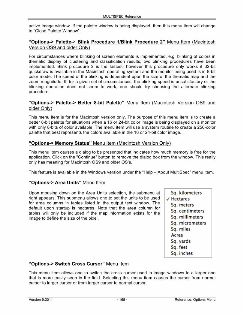
MULTISPEC Reference

Version 9.2011 - 168 - Reference: Options Menu

active image window. If the palette window is being displayed, then this menu item will change to “Close Palette Window”. “Options-> Palette-> Blink Procedure 1/Blink Procedure 2” Menu Item (Macintosh Version OS9 and older Only) For circumstances where blinking of screen elements is implemented, e.g. blinking of colors in thematic display of clustering and classification results, two blinking procedures have been implemented. Blink procedure 2 is the fastest; however this procedure only works if 32-bit quickdraw is available in the Macintosh operating system and the monitor being used is in 8-bit color mode. The speed of the blinking is dependent upon the size of the thematic map and the zoom magnitude. If, for a given set of circumstances, the blinking speed is unsatisfactory or the blinking operation does not seem to work, one should try choosing the alternate blinking procedure. “Options-> Palette-> Better 8-bit Palette” Menu Item (Macintosh Version OS9 and older Only) This menu item is for the Macintosh version only. The purpose of this menu item is to create a better 8-bit palette for situations when a 16 or 24-bit color image is being displayed on a monitor with only 8-bits of color available. The menu item will use a system routine to create a 256-color palette that best represents the colors available in the 16 or 24-bit color image. “Options-> Memory Status” Menu Item (Macintosh Version Only) This menu item causes a dialog to be presented that indicates how much memory is free for the application. Click on the "Continue" button to remove the dialog box from the window. This really only has meaning for Macintosh OS9 and older OS’s. This feature is available in the Windows version under the “Help – About MultiSpec” menu item. “Options-> Area Units” Menu Item Upon mousing down on the Area Units selection, the submenu at right appears. This submenu allows one to set the units to be used for area columns in tables listed in the output text window. The default upon startup is hectares. Note that the area column for tables will only be included if the map information exists for the image to define the size of the pixel. “Options-> Switch Cross Cursor” Menu Item This menu item allows one to switch the cross cursor used in image windows to a larger one that is more easily seen in the field. Selecting this menu item causes the cursor from normal cursor to larger cursor or from larger cursor to normal cursor.

MULTISPEC Reference

Version 9.2011 - 169 - Reference: Macintosh Window Menu

The Window Menu (Macintosh version) The items under this menu, shown to the right, allow one to hide and display selected windows and also to bring windows to the front of others. “Window-> Hide Window” Menu Item The "Hide Window" menu item causes the active window and all information in the window to be hidden. Hiding windows makes the screen appear less confusing. One can show a window again by selecting the window name in the last group at the bottom of the menu, if it is available (i.e. not shown in grayed form). “Window-> Show/Hide Coordinate View” Menu Item This menu item allows one to show or hide the coordinate view in the active image window. The coordinate view is above the image in the image window. The coordinate view displays the cursor location within the image, the start and end map information of the selected area and the image scale. See the "Coordinate View" discussion under MultiSpec Windows at the beginning of this Reference Section for further information. “Window – New Selection Graph” Menu Item The purpose of this menu item is to open a Selection Graph window. When one makes a selection within an image window, the average, plus and minus one standard deviation and the minimum and maximum values are plotted in the selection graph window as a response vs. channel number plot. If the selection represents only one pixel, only the values for that pixel are plotted. If the selection is for a thematic image window, the data value for the upper left pixel in the selection is plotted. The Selection Graph Window may be re-sized and moved on the screen in the usual manner. An example is shown in the “Windows” section of this reference. “Keeping” Selection Graph Windows

One can 'keep' selection graphs. If one selects the "New Selection Graph" again when a selection graph is already open, the contents of the current selection graph window is fixed and a new selection graph window is created. One can have up to 20 selection graph windows opened at any one time. Use the close box in the graph window or the “File-Close Window” menu item to close the window.

Printing Selection Graph Windows Graph windows can be printed by selecting the “File-Print Graph Window” menu item when the graph window is the active window. A graph window will be printed just as it is on the screen; the size will be the same.

MULTISPEC Reference

Version 9.2011 - 170 - Reference: Macintosh Window Menu

Copying Selection Graph Windows

One can also copy the graph window to the clipboard. After copying, the graph can then be pasted into another application such as a word processor. To copy a graph window, make it the active window, and then use the “Edit-Copy Graph” menu item or the COMMAND-C (Macintosh) or CONTROL-C (Windows) key combination. Note, if one is displaying graphs within the List Data processor then one must use COMMAND-C (Macintosh) or CONTROL-C (Windows) key combination to copy the graph window.

“Window – Text Output” Menu Item This menu item allows one to show the output text window if it is hidden and then bring it to the front position on the screen. “Window – Palette” Menu Item This menu item allows one to show the palette window if it is hidden and then bring it to the front position on the screen. “Window – Project” Menu Item This menu item allows one to show the project window if it is hidden and then bring it to the front position on the screen. “Window – ‘image or graph’ ” Menu Item This menu item allows one to show the selected image or graph window if it is hidden and then bring it to the front position on the screen. Each open image and graph window is listed in the Window Menu. The is indicated by its name printed in outlined characters. The active window (which may not be the active image window) is indicated by a check to the left of the window name.

MULTISPEC Reference

Version 9.2011 - 171 - Reference: Windows Window Menu

The Window Menu (Windows version) The items under this menu, shown to the right, allow one to arrange the windows, display selected windows and also to bring windows to the front of others. “Window-> New Window” Menu Item This menu item is not used in MultiSpec. “Window-> Cascade” Menu Item This menu item allows one to arrange the windows within the main MultiSpec window on top of each other with those on top being positioned slightly below and to the right of the window below it. “Window-> Tile” Menu Item This menu item allows one to arrange the windows within the main MultiSpec window in side by side fashion. “Window-> Arrange Icons” Menu Item This menu item allows one to automatically arrange any icons that represent MultiSpec windows. “Window-> Text Output” Menu Item This menu item allows one to show the text output window if it is an icon and then bring it to the front position on the screen. “Window-> ‘image or graph’ ” Menu Item This menu item allows one to show the selected image or graph window if it is an icon and then bring it to the front position on the screen. Each open image and graph window is listed in the Window Menu. The active window is indicated by a check to the left of the window name. “Window-> ‘project window’ ” Menu Item If the project window is open, then the menu item for it allows one to show the window if it is an icon and then bring it to the front position on the screen.

MULTISPEC Reference

Version 9.2011 - 172 - Reference: Shared Dialog Boxes

Shared Dialog Boxes The dialog boxes described below are used by more than one of the windows or menu items discussed above. The Select Channels Dialog Box

Channel List: This list allows one to select the channels (or features) to use. Click on the channel (or feature) to select it. The selected channels (or features) are highlighted. One can hold the shift or command key down when making selections to make multiple selections in the list. If this is a list of channels and the channel descriptions are available then the descriptions will be listed next to the channel number. Number selected: This information text line indicates how many items are currently selected in the list above. All: This button allows one to select everything in the list to the left. None: This button allows one to clear all of the selections in the list to the left. First, Last, Interval, Enter new range: The edit boxes allow one to select the first and last channel (or feature) in the list to the left plus an interval. The ‘Enter new range’ button allows one to enter the values specified in the edit boxes into the list. The list is updated automatically when one makes changes in the edit boxes. The ‘Enter new range’ button is useful, if one uses the ‘All’ or ‘None’ buttons and then one wants to change the list back to those specified in the edit boxes. Cancel: This button closes the dialog box and cancels the ‘Select Channels’ request. OK: This button closes the dialog box and sets the channels (or features) to use setting to that specified in the dialog box. For example, in the list above, channels 3 through 7 have been selected. This set will also be the default subset for other processors.

MULTISPEC Reference


The Select Classes Dialog Box

Class List: This list allows one to select the classes to use. Click on the class name to select it. The selected classes are highlighted. One can hold the shift or command key down to make multiple selections in the list. Number selected: This information text line indicates how many items are currently selected in the list above. All: This button allows one to select everything in the list to the left. None: This button allows one to clear all of the selections in the list to the left. First, Last, Interval, Enter new range: The edit boxes allow one to select the first and last class in the list to the left plus an interval. The ‘Enter new range’ button allows one to enter the values specified in the edit boxes into the list. The list is updated automatically when one makes changes in the edit boxes. The ‘Enter new range’ button is useful, if one uses the ‘All’ or ‘None’ buttons and then one wants to change the list back to those specified in the edit boxes. Cancel: This button closes the dialog box and cancels the ‘Select Classes’ request. OK: This button closes the dialog box and sets the classes to use setting to that specified in the dialog box. For example, in the list above, classes 3 through 9 have been selected. Other Notes: The default subset will be the class selected in the project window if the project window is open and a class is selected in it.

MULTISPEC Reference


The Specify Class Weights Dialog Box

Class: This list allows one to select the class whose weighting value is to be changed. Click on the class name to select it. The selected classes are highlighted. One can hold the shift or command key down to make multiple selections in the list.

Enter New Weight: This button and edit box allow one to specify the weight value for the selected class(es) in the list above and to then enter that value into the list.

Add to Equal Weight Set: This button allows one to force the weight for the selected class(es) to be that used for an ‘equal’ class weight.

Units: This information indicates that the weight values should be considered as relative to each other. If one class has a weighting value of 10 and another has a value of 5 then the first class should be treated as having double the weight of the second class. (Some thought has been given to doing the weights as a percent, but that capability has not been implemented.)

Weight Total: This information text line indicates what the current total is for the weight values in the list to the left.

Help…: This button allows one to open a dialog box which describes how to use the ‘Specify Class Weights’ dialog box.

Cancel: This button closes the dialog box and cancels the ‘Specify Class Weights’ request.

OK: This button closes the dialog box and sets the class weights to those specified in the dialog box.

The procedure to determine the actual weight ratio to use in the algorithms is to compute the sum of the weight values in the list (the weight total) and then divide the weight value in the list for each class by the total. This guarantees that the sum of the weight ratios will be 1.

MULTISPEC Reference


The Specify Class Pair Weights Dialog Box

Class List: This list allows one to select the classes whose between class weighting value is to be changed. Click on the class name to select it. The selected classes are highlighted. One can hold the shift or command key down to make multiple selections in the list. One may wish to set between class weights to 0 for those spectral class which represent the same information group and one does not care separating them. Classification errors between them is no problem.

Default weight: This edit box allows one to set the weight value to use as the default weighting between classes.

New Weight: This edit box allows one to specify the weight value to use between the classes selected in the list to the left.

Add: This button allows one to set the ‘between or interclass class weighting’ for the selected classes in the list to the left to the value entered in the edit box above. After selecting this button, a line will be entered in the list to the right listing the class pair weighting value and the class pairs that the value will be used for. If more than two classes in the list to the left are selected, then the weight value will be used for all class pair combinations in the selected classes.

Remove: This button allows one remove the selected class pair weighting set(s) in the list to the right.

Help…: This button allows one to open a dialog box which describes how to use the ‘Specify Class Pair Weights’ dialog box.

Wt. - Class Pairs: This list indicates the class pairs that have interclass weighting values that have been set by the user. Click on a line in the list to select it; the selected lines are highlighted. One can hold the shift or command key down to make multiple selections in the list.

Cancel: This button closes the dialog box and cancels the ‘Specify Class Pair Weights’ request.

OK: This button closes the dialog box and sets the class pair weights to those specified in the dialog box.

MULTISPEC Reference


The Assign Channels for False Color Palette Dialog Box

This dialog box allows one to select the channels in each class mean vector to define the red, green and blue value for each thematic color. For example one could assign channels 4, 3, and 2 to red, green and blue, respectively, for Thematic Mapper data to obtain class colors very similar to a multispectral color IR image of the data. Classes that are close to each other in spectral space for the three selected channels will have similar colors. Note that an open project file is required. Red, Green, Blue: These edit boxes allow one to select the channel to be used in the mean vector for each class to define the Red, Green, and Blue value in the respective thematic color palette. Available Channels: This list allows one to view the list of available channels and channel descriptions for reference if needed. Cancel: This button closes the dialog box and cancels the ‘Assign Channels for False Color Palette’ request. OK: This button closes the dialog box and sets channels to be used in each class mean vector to define the palette colors for each class.

MULTISPEC Reference


The Change Class Symbols Dialog Box (Macintosh Version Only)

This dialog box allows one to assign a symbol to represent a given class. Symbol-Class name: This list allows one to select the class to which a different symbol is to be assigned. The symbol to the left is the one that is currently assigned to the class. The selected class or classes are highlighted. New Symbol: This edit box contains the symbol that is selected in the list to the right or one can enter a value between 0 and 9 into the box. <-: This button allows one to assign the selected symbol in the New Symbol edit box to the selected class or classes in the list to the left. Symbols: This list contains all the symbols that are available to be assigned to a class. In the case above, the symbol ‘a’ has been selected. Help…: This button allows one to open a dialog box which describes how to use the ‘Change Class Symbols’ dialog box. Cancel: This button closes the dialog box and cancels the Change Class Symbols’ request. OK: This button closes the dialog box and sets the class symbols to those specified in the dialog box.

MULTISPEC Reference

Version 9.2011 - 178 - Reference: General Characteristics

General Characteristics of MultiSpec Under the Apple Macintosh Operating System MultiSpec supports the high level Apple Events. The Apple Events that MultiSpec currently supports are the four required events: open application, open document, print document, and quit application. Apple's Balloon Help capability for versions supporting Operating Systems 7-9 has been implemented for the menu items. Balloon Help is not a part of OSX. One can put MultiSpec in the background when one is displaying an image. Both the short status dialogs (as used in the Reformat processor) and the long status dialogs (as used in the Classify processor) are moveable if MultiSpec is being run under the Macintosh Operating System 7 or later. If a status dialog box is being displayed, the user has access to the application menu or dock to place MultiSpec in the background. Generally speaking the cancel button is checked every 1-2 seconds so that there may be some delay in the actual cancel operation. "Popup menus" type are indicated by the symbol. "Mousing down" on them results in a menu appearing allowing for the selection of allowed values of those parameters. All computations in the MultiSpec are done with 19-digit precision for Motorola 680x0 based machines and 15-digit precision for IBM/Motorola PowerPC and Intel based machines.

Introduction to MULTISPEC - Appendices

Version 9.2011 - 179 - Appendix A. Project File Format

APPENDIX A. PROJECT FILE FORMAT Versions 890105, 900508, 911106, 920226, 930226, 940105, 971008, 990107, 20060124, 20110722. Descriptions of the format of each line in the project files follow. The item given between the single quotes are exact descriptions of what is in the field or parameter. '\t' refers to a tab and '\r' refers to a carriage return. The information between () to the right of each parameter is the 'C' format that was used to write the value to the project file. Project format description line. MultiSpec project format file identifier. 'PROJECT FORMAT VERSION' Project format version identifier. '890105' or '900508' or '911106' or '920226' or '930226' or '940105' or '971008' or '990107' or ‘20060124’ or ‘20110722’ Filler ' 1\r' or '0\r' or '0\r' or '0\r' or '0\r' or '0\r' Project information lines. P1 line. 'P1 PROJECT NAME\t' number of characters in project name, '\t' - (%d) project name, '\t' - (%s) number of characters in base image file name, '\t' - (%d) base image file name, '\r' - (%s) P2 line

'P2\t' number of lines in base image file, '\t' - (%ld) number of columns in base image file, '\t' - (%ld) number of channels in base image file, '\t' - (%hd) number of bytes in data values in base image file, '\t' - (%hd) start line of base image file, '\t - (%ld) (900508 and later

versions) start column of base image file, '\t - (%ld) (900508 and later

versions) number of bits per data value in base image file, '\t'-(%hd) (911106 and later versions) swap bytes flag, '\t'-(%hd). 0=no, 1=yes. (911106 and later versions) band interleave code, '\t'-(%hd). 1=BIL, 2=BSQ, 3=BIS. (911106 and later versions) number of header bytes, '\t'-(%ld) (911106 and later versions) number of trailer bytes, '\t'-(%ld) (911106 and later versions) number of preline bytes, '\t'-(%ld) (911106 and later versions) number of postline bytes, '\t'-(%ld) (911106 and later versions) number of classes, '\t' - (%hd) number of classes with training field, '\t' - (%hd) number of fields, '\t' - (%hd) number of training fields, '\t' - (%hd) number of test fields, '\t' - (%hd) number of coordinates that define the fields, '\t' - (%hd) number of statistics channels, '\t' - (%hd) flag indicating whether computed statistics for the project are up-to-date, '\t' - (%hd). 0 = no, 1 = yes.



code indicating the type of statistics computed for the project, '\t' - (%hd). 1 = mean & standard deviation only. 2 = mean, standard deviation, and covariance.

(920226 and later versions) flag indicating whether only the class statistics are saved instead of the field statistics, '\t' - (%hd) . 0 = no, 1 = yes. (930226 and later versions) flag indicating whether the data are to be treated as signed data (=1) or unsigned data (=0). '\t' - (%hd) . (971008 and later versions) flag indicating whether the common covariance is to be used when computing the leave-one-

out covariance. '\t' - (%hd). 0 = no, 1 = yes. (971008 and later versions) code indicating which covariance statistics to use. '\t' - (%hd). 1 = original, 2 = leave-one-out,

4 = enhanced statistics, 8 = mixed statistics. (971008 and later versions) code indicating the data type for the base image. ‘\t’ - (%hd). 0 = integer, 1 = real. (20060124

and later versions) data set number being used in hdf formatted files for the base image. ‘t’ - (%hd) -‘\r’.

(20060124 and later versions) code indicating machine architecture used to write the file. Important to know for binary

modified statistics. ‘t’ - (%hd) -‘\r’. 1 = Macintosh PPC (big endian), 2 = Macintosh Intel (little endian), 3 = Windows Intel (little endian) (20110722 and later versions)

P3 line

'P3\t' channel numbers separated by tabs, '\t', and ending with a carriage return, '\r' - (%d).

P4 line (990107 and later versions) 'P4 TRAINING MASK NAME\t' number or characters in training mask file name\t '1' P5 line (990107 and later versions) 'P5 TEST MASK NAME\t' number of characters in test mask file name\t '1' Line indicating start of training statistics. 'Training Statistics\r' Class information. There will be one set of the following information for each class in the project. Note that beginning with the 920226 version, the class statistics will be computed by summing the field statistics if the class statistics lines are not present. This was done to reduce the size of the project. If the statistics for a field have not been computed, then the FS and FSS lines are not required. C1 - required. CM - optional for 920226 and later versions. CS - optional for 920226 and later versions. CCV - optional for 920226 and later versions. CSS - optional for 920226 and later versions. CEM - optional for 940105 and later versions. CEC - optional for 940105 and later versions. F1 - required. One for each field in the class. FS - required if computed. One for each field in the class. FSS - required if computed. One for each field in the class. FM - required if computed. One for each field in the class. FN - required if computed. One for each field in the class. FCV - optional for 920226 and later versions. FX - optional for 920226 and later versions. V1- required. One set for each field in the class.



C1 line. 'C1\t' number of characters in the class name, '\t' - (%d) class name, '\t' - (%s) number of fields in the class, '\t' - (%d) number of training fields in the class, '\t' - (%d) number of test fields in the class, '\t' - (%d) total number of training pixels in the class, '\t' - (%d) flag indicating whether the computed statistics for the class are up-to-date, '\t' - (%d) 0 = no, 1 = yes. flag indicating if enhanced statistics exist for the class, '\t' - (%d) 0 = no, 1 = yes. (940105 and later versions) prior weighting for original statistics, '\t' - (%f) (940105 and later versions) prior weighting for enhanced statistics, '\t' - (%f) - '\r' (940105 and later versions) weighting for computing common covariance, '\t' - (%f) - '\r' (971008 and later versions) leave-one-out covariance value, '\t' - (%f) - '\r' (971008 and later versions) code indicating covariance statistics to use for class. '\t' - (%d) - '\r'. 1 = original, 2 = leave-

one-out, 4 = enhanced statistics. (971008 and later versions)

CM line - Channel means for the class. 'CM\t' channel means separated by tabs,'\t'. The last channel mean is followed by a carriage

return,'\r'. - (%.9g)

CS line. Sums of the data values for each channel in the class. 'CS\t' channel sums separated by tabs,'\t'. The last channel sum is followed by a carriage return,'\r'.

- (%.0f)

CCV lines. The covariance matrix for the class is written in lower triangular form. 'CCV\t' covariance values separated by tabs,'\t'. The last covariance value for each line in the lower

triangular matrix is followed by a carriage return,'\r'. - (%.9g)

CSS lines. A matrix of the sum of the squares of the data values for the class is written in lower triangular form.

'CSS\t' sum of square values separated by tabs,'\t'. The last value for each line in the lower triangular

matrix is followed by a carriage return,'\r'. - (%.0f)

CEM line - Enhanced channel means for the class. 'CEM\t' The enhanced channel means are written in 8-byte double binary form. The last channel

mean is followed by a carriage return,'\r'.

CEC lines - The enhanced covariance matrix for the class is written in lower triangular form. 'CEC\t' The enhanced values are written in 8-byte double binary form. The last enhanced value for

each line in the lower triangular matrix is followed by a carriage return,'\r'. Field information. There will be one set of the following information for each training field in the class - lines F1, FM, FS, FCV, FSS, and V1. F1 line

'F1\t' number of characters in the field name, '\t' - (%d) field name, '\t' - (%s) number of coordinate points that describe the field , '\t' - (%d) class number that the field belongs to, '\t' - (%d)



code for the field type, '\t' - (%d). 1=training, 2=testing. code for the coordinate type, '\t' - (%d). 1=rectangular, 2=polygonal, 3=cluster, 4=mask total number of pixels in the field, '\t' - (%d) flag indicating whether the statistics for this field have been loaded into the class statistics, '\t'

- (%d) flag indicating whether the computed statistics for the field are up-to-date, '\r' - (%d) mask value for field if any, '\t' - (%d). (990107 and later versions)

FM line - Channel means for the field. If the statistics have not been computed for the field yet, this line will not be included.

'FM\t' channel means separated by tabs, '\t'. The last channel mean is followed by a carriage return,

'\r'. - (%.9g)

FN line - Channel minimums for the field. If the statistics have not been computed for the field yet, this line will not be included.

'FN\t' channel minimums separated by tabs, '\t'. The last channel mean is followed by a carriage

return, '\r'. - (%d)

FX line - Channel maximums for the field. If the statistics have not been computed for the field yet, this line will not be included.

'FX\t' channel maximums separated by tabs, '\t'. The last channel mean is followed by a carriage

return, '\r'. - (%d)

FS line. Sums of the data values for each channel in the field. If the statistics have not been computed for the field yet, this line will not be included.

'FS\t' channel sums separated by tabs, '\t'. The last channel sum is followed by a carriage return,

'\r'. - (%.0f)

FCV lines. The covariance matrix for the field is written in lower triangular form. If the statistics have not been computed for the field yet, this line will not be included.

'FCV\t' covariance values separated by tabs, '\t'. The last covariance value for each line in the lower

triangular matrix is followed by a carriage return, '\r'. - (%.9g)

FSS lines. A matrix of the sum of the squares of the data values for the field is written in lower triangular form. If the statistics have not been computed for the class yet, this line will not be included.

'FSS\t' sum of square values separated by tabs, '\t'. The last value for each line in the lower

triangular matrix is followed by a carriage return,'\r'. - (%.0f)

Coordinate description of the field.

V1 lines. There will be one 'V1' line for each one of the coordinate points that describe the field. If the point type is 'rectangular', point type = 1, then two coordinate points are given - the upper left corner and the lower right corner. If the point type is 'polygonal', point type = 2, then a coordinate point is given for each vertex of the polygon.

'V1\t' line number of coordinate, '\t' - (%d) column number of coordinate, '\r' - (%d) "Sets of information for rest of training fields for the class" . . "Sets of information for rest of classes in the project"



. . . Line indicating start of test field information. 'Test Fields\r' Test field information. There will be one set of the following information for each test field in each of the classes - lines F1 and V1. F1 line - See description for 'F1' line above. V1 lines - See description for 'V1' lines above. An example project file follows: PROJECT FORMAT VERSION 20110722 0 P1 PROJECT NAME 25 TIPJUL1_for_intro.Project 11 TIPJUL1.LAN P2 169 169 7 1 1 3 8 0 1 128 0 0 0 2 2 4 2 2 15 7 1 2 1 0 1 1 0 0 2 P3 1 2 3 4 5 6 7 Training Statistics C1 4 Corn 2 1 1 144 1 0 10.000000 10.000000 10.000000 -1.000000 1 CS 12018 4459 3801 17543 10789 2966 21107 CN 80 29 24 112 69 15 145 CX 88 35 29 129 108 41 148 CSS 1003294 CSS 372184 138203 CSS 317279 117741 100545 CSS 1464116 543289 462983 2138259 CSS 900849 334587 285345 1314393 814529 CSS 247764 92113 78576 361294 225408 63060 CSS 1761568 653591 557148 2571366 1581562 434828 3093835 F1 7 Field 1 2 1 1 1 144 1 0 0 V1 34 35 V1 49 43 C1 9 Bare Soil 2 1 1 86 1 0 10.000000 10.000000 10.000000 -1.000000 1 CS 8517 3564 3931 7404 11900 5896 13195 CN 90 34 34 55 86 39 152 CX 111 50 59 114 166 86 155 CSS 845077 CSS 354120 148716 CSS 391161 164451 182271 CSS 737627 310630 344176 655830 CSS 1184074 497839 551409 1045113 1674228 CSS 586962 246876 273675 518406 830855 412944 CSS 1306810 546860 603207 1136107 1826141 904815 2024561 F1 7 Field 2 3 2 1 2 86 1 0 0 V1 74 63 V1 72 78 V1 84 76 Test Fields F1 7 Field 3 4 1 2 2 146 0 0 0 V1 35 7 V1 33 16 V1 49 16 V1 49 5 F1 7 Field 4 2 2 2 1 150 0 0 0 V1 5 142 V1 19 151


Version 9.2011 - 184 - Appendix B. MultiSpec Limits

APPENDIX B. MULTISPEC LIMITS Some of the limits for MultiSpec are described below. In most cases the limits are high enough so that the real limits are memory, disk space and time. Please let us know if any of these limits cause any problems. Image File Description Maximums number of lines - 200,000 number of columns - 200,000 number of channels - 8,192 (Multispectral) number of unique classes numbers - 65,535 (Thematic) start line - 2,147,483,647 start column - 2,147,483,647 header bytes - 2,147,483,647 trailer bytes - 2,147,483,647 pre-line bytes - 2,147,483,647 post-line bytes - 2,147,483,647 pre-channel bytes - 2,147,483,647 post-channel bytes - 2,147,483,647 maximum file size (bytes) - 2,147,483,647 maximum number of integer data value bytes - 4 maximum number of integer data value bits - 32 minimum integer data value - -2,147,483,648 maximum integer data value - 4,294,967,295 maximum number of real data value bytes - 8 maximum number of real data value bits - 64 smallest real data value - 2.2250738585072014e-308 maximum real data value - 1.7976931348623157e+308 Displayable Limits number of lines - 32,767 number of columns (B/W pattern, 8-bit color) - (Macintosh Version) 16,376 (Windows 16-bit Version) 8,188 (Windows 32-bit Version) 32,767 number of columns (24-bit color) - (Macintosh Version) 4,094 (Windows 16-bit Version) 21,844 (Windows 32-bit Version) 32,767 maximum magnification - 99 minimum magnification - 0.01 number of classes (Thematic display) - 65,535 Project Maximums number of statistics channels - 8192 number of classes - 255 total number of fields - 32,767 number of fields per class - 512 total number of points to describe fields - 32,767


Version 9.2011 - 185 - Appendix C. Transformation File Format

APPENDIX C. TRANSFORMATION FILE FORMAT The transformation file format is: Bytes 1-256 bytes: Image file name in pascal format (i.e. first byte is number of characters in the

name. (ASCII characters) Bytes 257-258: Number of channels in transformation. (2-byte integer) Byte 259: The Endianness Code [highest 4-bits; 0=Unknown, 1=Big Endian, 2-Little Endian] and

File Format Version Number [lowest 4-bits; 0, 1, 2, 3=current version beginning on 9/2/2011]. (1-byte integer)

Byte 260: Created-by code. Principal Component =1, Feature Extraction =2, Feature Extraction

with preprocessing =21. (1-byte integer) Bytes 261-262: Number of features. (2-byte integer) Bytes 263-263+numberChannels*2: List of channels that were used. (2-byte integer for each

channel) Next group of bytes: If the Created-by code =21, then this is the preprocessing channel

grouping. It is numberFeatures * 2 bytes long. (2-byte integer for each channel) Next group of bytes: Eigenvalues. This is numberFeatures*(size-of-double) bytes long. [In the

Macintosh (non-carbon or OSX) versions, this is in 68881 double format which is 96 bits (10 bytes) long. In the Carbon and OSX Macintosh versions and in the Windows version, this is in double format which is 64 bits (8 bytes) long. The current versions of the transformation files are cross-platform compatible.]

Next group of bytes: Principal Component Means. This is numberFeatures*(size-of-double)

bytes long. [See description above for eigenvalues] Next group of bytes: Eigenvectors. This is numberFeatures*numberChannels* (size-of-double)

bytes long. [See description above for eigenvalues].

The order of the eigenvectors: There are "numberFeatures" eigenvectors with "numberChannels" components in each one. The order of them in the file is the first component for each of the eigenvectors, then the second component, then the third, etc. This is the transpose of how the eigenvectors are listed by MultiSpec in the output text window, if you think of memory being connected across a line of text.


Version 9.2011 - 186 - Appendix D. Gain-Offset Transformation File Format

APPENDIX D. GAIN-OFFSET TRANSFORMATION FILE FORMAT A gain-offset transformation can be used to apply a gain and offset adjustment to each channel in the image data. For example, it can apply a flat field adjustment to image data to convert the data from apparent radiance units to apparent reflectance or vice versa. One can use the “File – Load Transformation Matrix” menu item to load the transformation into memory. Use the “Reformat-Change Image File Format” menu item to apply the transformation when creating a new image file. One can verify that the transformation loaded properly using the “Processor-Utilities-Check Transformation Matrix” menu item. The format of the offset-gains type of transformation file is:

line 1: 'Offsets-Gains' line 2: 'Current=New' or 'New=Current' line 3: number of channels in the file, one per line, (%ld) line 4: scale factor to multiply final value by after offset-gain adjustment, (%ld) line 5 to end: one line for each channel contain the offset as first value, and the gain as the

second value. Other values can be in the line such as channel number, but they will be ignored.

If the file is a 'Current=New' type of file, the new value is computed as:

new = scale factor * (old value - offset)/gain If the file is a 'New=Current' type of file, the new value is computed as:

new = scale factor * (offset + gain*old value) The scale factor can be used to scale the data so that one keeps a specified amount of precision. For example, if the transformation causes the data to be scaled from 0 to 1, one may want to use 100 to re-scale the data from 0 to 100 or 1000 to re-scale the data from 0 to 1000 before rounding to an integer value which the Reformat - Change Image File Format option does. An example file is: Offsets-Gains Current=New 7 100 1298.14 8498.14 1 1336.84 8920.26 2 1246.94 8410.39 3 1185.94 8512.11 4 1240.09 8538.67 5 1232.11 8620.57 6 1219.22 8933.45 7


Version 9.2011 - 187 - Appendix E. Image File Format Notes

APPENDIX E. Image Format Notes The following is a list of the image file formats that MultiSpec can handle:

Arc Info Binary Grid, ArcView, ArcView Shape File Enhanced Compression Wavelet (ECW). ENVI, ERDAS *.LAN, ERDAS *.GIS, ERDAS Imagine (uncompressed) FastL7A, GAIA, GeoTIFF & TIFF uncompressed, Gridded Binary (GRIB), HDF4 - Scientific Data Model, JPEG2000, Land Analysis System (LAS), LARSYS Multispectral Image Storage Tape (MIST), LGSOWG, MacSADIE, MultiSpec ASCII classification formatted data files, NetCDF, NLAPS Data Format (NDF), PDS, PNG, Sun "Screen Dump", TARGA uncompressed, VICAR Windows Bit Map (BMP)

The following are some details about some of the image data formats specific to how MultiSpec handles them. ERDAS IMAGINE

MultiSpec cannot handle Imagine formatted files with compressed data. MultiSpec can handle the ERDAS Imagine .ige (spill) files. These files are used for images with more than 2 gigabytes of data.

HDF4

MultiSpec can read compressed data in HDF4 formatted files. Several of the hdf4 data sets that NASA now produces contain compressed data.

NLAPS Data Format (NDF)

MultiSpec will automatically link the separate band files together if one selects the H1, H2, H3 and HD header files. One can then use the Processor-> Reformat-> Change Image File Format menu item to save a combined image to disk. If one selects the I1, I2, I3, etc suffix files, then only that one band will be opened. For Landsat 5 data, MultiSpec links the bands together in wavelength order.


Version 9.2011 - 188 - Appendix E. Image File Format Notes

TIFF/GeoTIFF

Candidate TIFF images must not be 1 bit and must not be in a compressed format. Those TIFF images with color tables are treated as Thematic type images and those TIFF images with 1 or more layers (or channels) and no color table are treated as Multispectral type images. MultiSpec will read the control points that may be stored in GeoTIFF images and use them to define a polynomial transformation to translate between line/column value to map/latitude-longitude value when no other map projection information exists. This has been used for the Level 1A SPOT images to be able to display an estimate of the latitude-longitude values in the coordinate window and to overlay latitude-longitude shape files. Three control points must be available before they are used. The control points are written to geotiff images that MultiSpec generates if they are available. An order 1 polynomial is used for 3 thru 5 controls points, order 2 for 6 thru 9 control points and order 3 is used for 10 or more control points. The control point information is displayed when one lists the image description information. Note that when writing an image with an orientation angle, such as many ASTER files, to a GeoTIFF file, the orientation angle is not included in the output file. One will have to note what the orientation angle is and enter the value again if read back into MultiSec or other applications.


Version 9.2011 - 189 - Appendix F. ʻ.clrʼ File Format

APPENDIX F. ‘.clr’ File Format The ‘.clr’ file defines the colors to be used for each of the data values in a thematic image file. The format is the same as that for an Arc View .clr file with additional information for each thematic data value that also defines the class name to associate with the data value and color and name for information groups associated with each thematic data value. The .clr file can still be read as a ArcView .clr file by other applications. An example .clr file follows. 0 255 255 255 n:background~ g:0 255 255 255 background~ 1 255 254 137 n:Alfalfa~ g:1 255 254 137 Forage/Hay~ 2 3 28 241 n:Br Soil~ g:2 153 102 51 Br Soil~ 3 255 89 1 n:Corn~ g:3 255 89 1 Row Crops~ 4 5 255 133 n:Oats~ g:4 5 255 133 Small Grains~ 5 255 2 251 n:Red Clover~ g:1 6 89 1 255 n:Rye~ g:4 7 3 171 255 n:Soybeans~ g:3 8 12 255 7 n:Water~ g:5 0 0 255 Water~ 9 172 175 84 n:Wheat~ g:4 10 160 78 158 n:Wheat-2~ g:4 The description for the above information in order of data value or text info is: - Data value for the thematic class in the associated image file - Red color value (number between 0 and 255) - Green color value (number between 0 and 255) - Blue color value (number between 0 and 255)

Note that the following is specific for MultiSpec: - n:name for this thematic data value; ‘~’ is the terminator for the name. The limit for the name is

31 characters.

The following is only needed if one wishes to have information groups. Note that the group color and group name only need to be listed one time.

- G:nn is the information group category that the thematic value belongs to where nn is group

number. - Red color value for information group (number between 0 and 255) - Green color value for information group (number between 0 and 255) - Blue color value for information group (number between 0 and 255) - Name for information group; ‘~’ is the terminator for the name. The limit for the name is 31

characters.

Documents

An Introduction & Reference For - Purdue Engineeringbiehl/MultiSpec/MultiSpec_Intro_9... · An Introduction & Reference For MultiSpec© Version 9.2011 Program Concept and Introduction