An Introduction into Stress-Life Fatigue Techniques

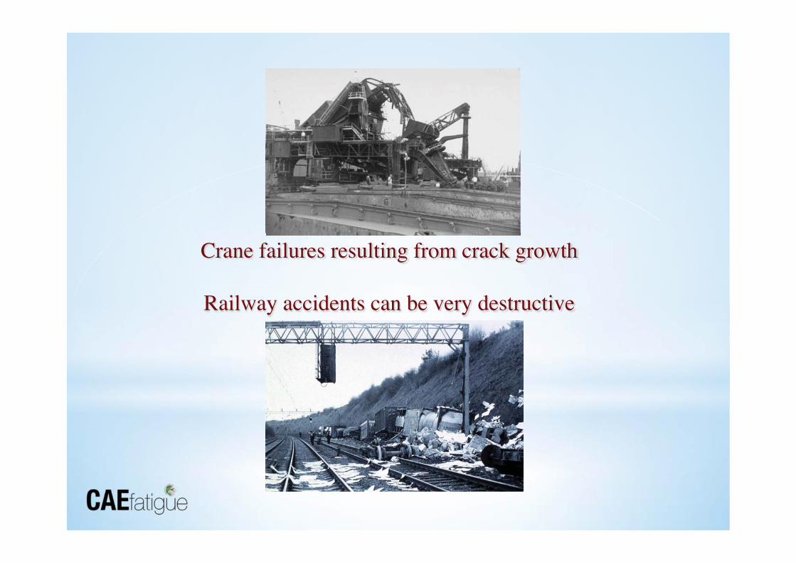
Crane failures resulting from crack growth

Railway accidents can be very destructive

What is Fatigue?

•  Fatigue is: –  “Failure” under a repeated or otherwise

varying load which never reaches a level sufficient to cause failure in a single application. (deformation based approach)

–  The growth of an existing crack, or growth from a pre-existing material defect, until it reaches a critical size. (material behavior based approach)

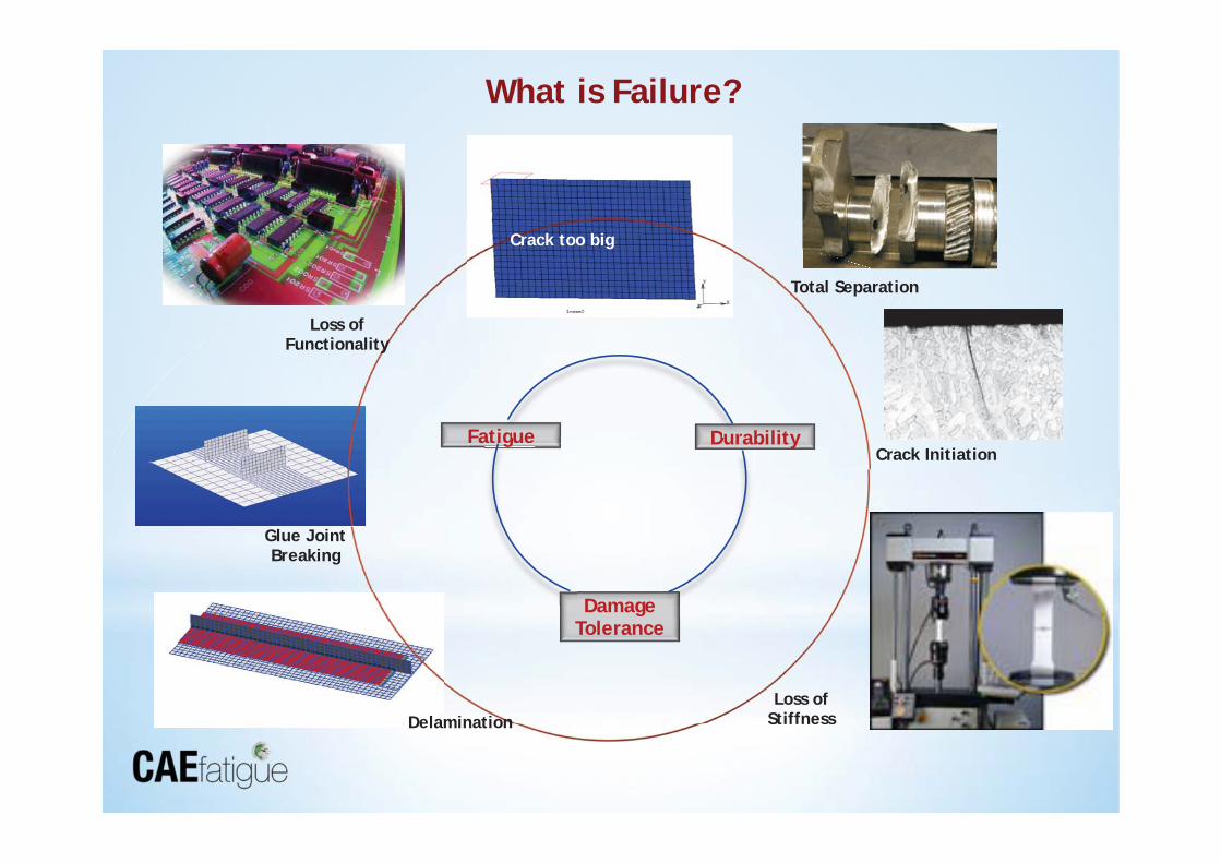
What is Failure?

Crack too big

Crack Initiation

Glue Joint Breaking

Loss of Stiffness Delamination

Loss of Functionality

Durability Fatigue

Damage Tolerance

Durgueg

Total Separation

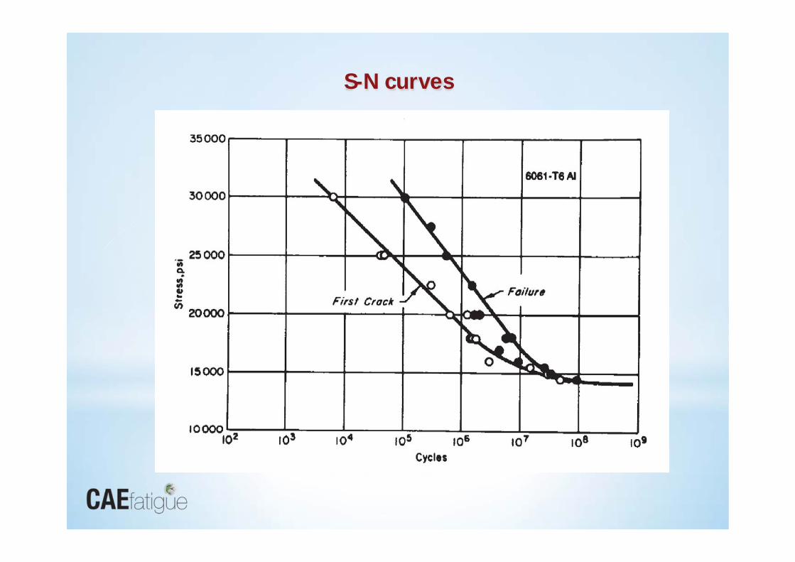
S-N curves

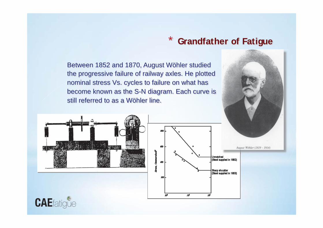
*  Grandfather of Fatigue

Between 1852 and 1870, August Wöhler studied the progressive failure of railway axles. He plotted nominal stress Vs. cycles to failure on what has become known as the S-N diagram. Each curve is still referred to as a Wöhler line.

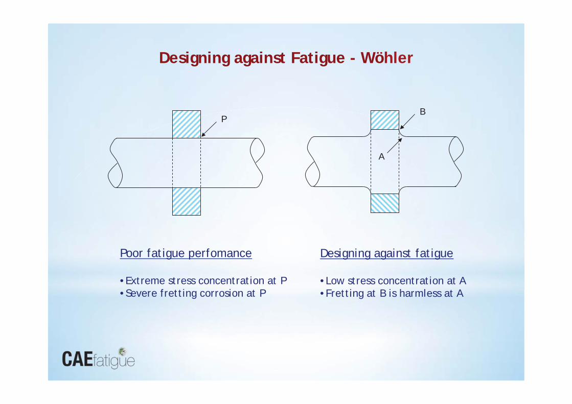
Designing against Fatigue - Wöhler

Poor fatigue perfomance • Extreme stress concentration at P • Severe fretting corrosion at P

Designing against fatigue • Low stress concentration at A • Fretting at B is harmless at A

P B

A

Example: Using Paper Clips to Generate an S-N Curve

Take 5 paper clips each

Group 1 - apply 45 degree repeated strains

Group 2 - apply 90 degree repeated strains

Plot results on S-N curve

Estimate scatter and discuss!

Load or displacement control?

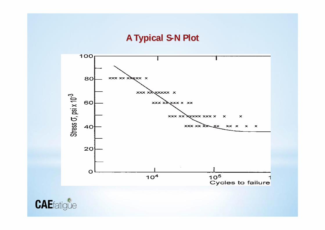
A Typical S-N Plot

Fatigue Technology...

  Is very old technology (40-160 years old);

  Is a collection of empirical rules that were induced to fit observed behaviour and are generally accepted to work;

  The designer, or engineer, wishing to exploit it should be familiar with the concepts but not necessarily all of the theories

•  S-N (Stress-Life) Relates nominal or local elastic stress to fatigue life

•  ε-N (Strain-Life)

Relates local strain to fatigue life

•  LEFM (Crack propagation) Relates stress intensity to crack propagation rate

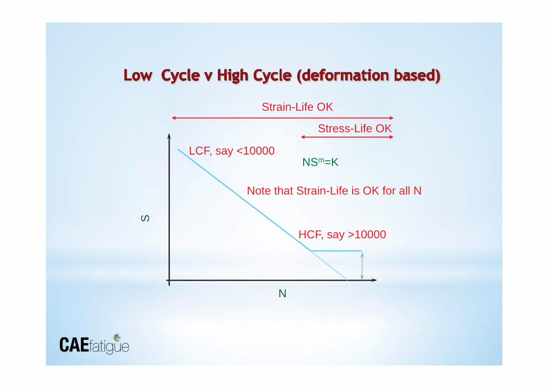
S

N

NSm=K LCF, say <10000

HCF, say >10000

Note that Strain-Life is OK for all N

Strain-Life OK

Stress-Life OK

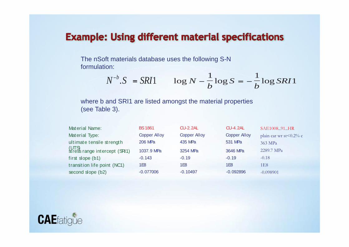
The nSoft materials database uses the following S-N formulation:

where b and SRI1 are listed amongst the material properties (see Table 3).

N S SRIb− =. 1 log log logNb

Sb

SRI− = −1 1

1

Material Type:

Copper Alloy

Copper Alloy

Copper Alloy

ultimate tensile strength (UTS)

206 MPa

435 MPa

531 MPa

stress range intercept (SRI1)

1037.9 MPa

3254 MPa

3646 MPa

first slope (b1)

-0.143

-0.19

-0.19

transition life point (NC1)

1E8

1E8

1E8

Material Name:

BS 1861

CU-2.2AL

CU-4.2AL

second slope (b2)

-0.077006

-0.10497

-0.092896

SAE1008_91_HR plain car wr st<0.2% c 363 MPa 2289.7 MPa -0.18 1E8 -0.098901

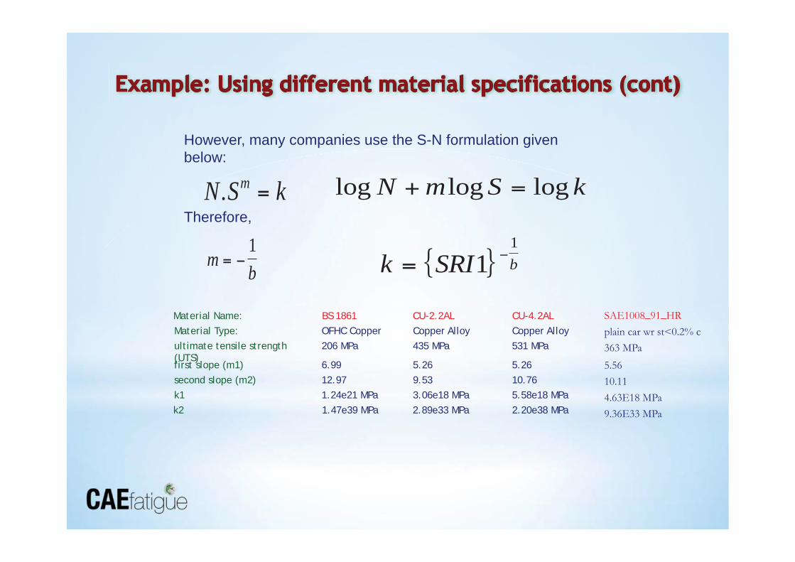
However, many companies use the S-N formulation given below:

N S km. = log log logN m S k+ =

mb

= −1

{ }k SRI b= −11

Therefore,

Material Type:

OFHC Copper

Copper Alloy

Copper Alloy

ultimate tensile strength (UTS)

206 MPa

435 MPa

531 MPa

first slope (m1)

6.99

5.26

5.26

second slope (m2)

12.97

9.53

10.76

k1

1.24e21 MPa

3.06e18 MPa

5.58e18 MPa

Material Name:

BS 1861

CU-2.2AL

CU-4.2AL

k2

1.47e39 MPa

2.89e33 MPa

2.20e38 MPa

SAE1008_91_HR plain car wr st<0.2% c 363 MPa 5.56 10.11 4.63E18 MPa 9.36E33 MPa

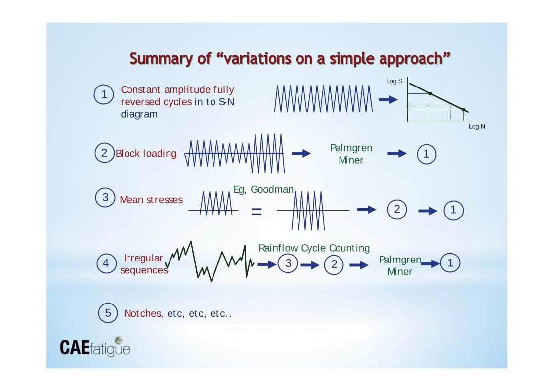
Constant amplitude fully reversed cycles in to S-N diagram

Log S

Log N

1

3 Mean stresses = 1

2

2

1

4 3 2 Palmgren Miner

1

5 Notches, etc, etc, etc..

Rainflow Cycle Counting

Block loading

Irregular sequences

Palmgren Miner

Eg, Goodman

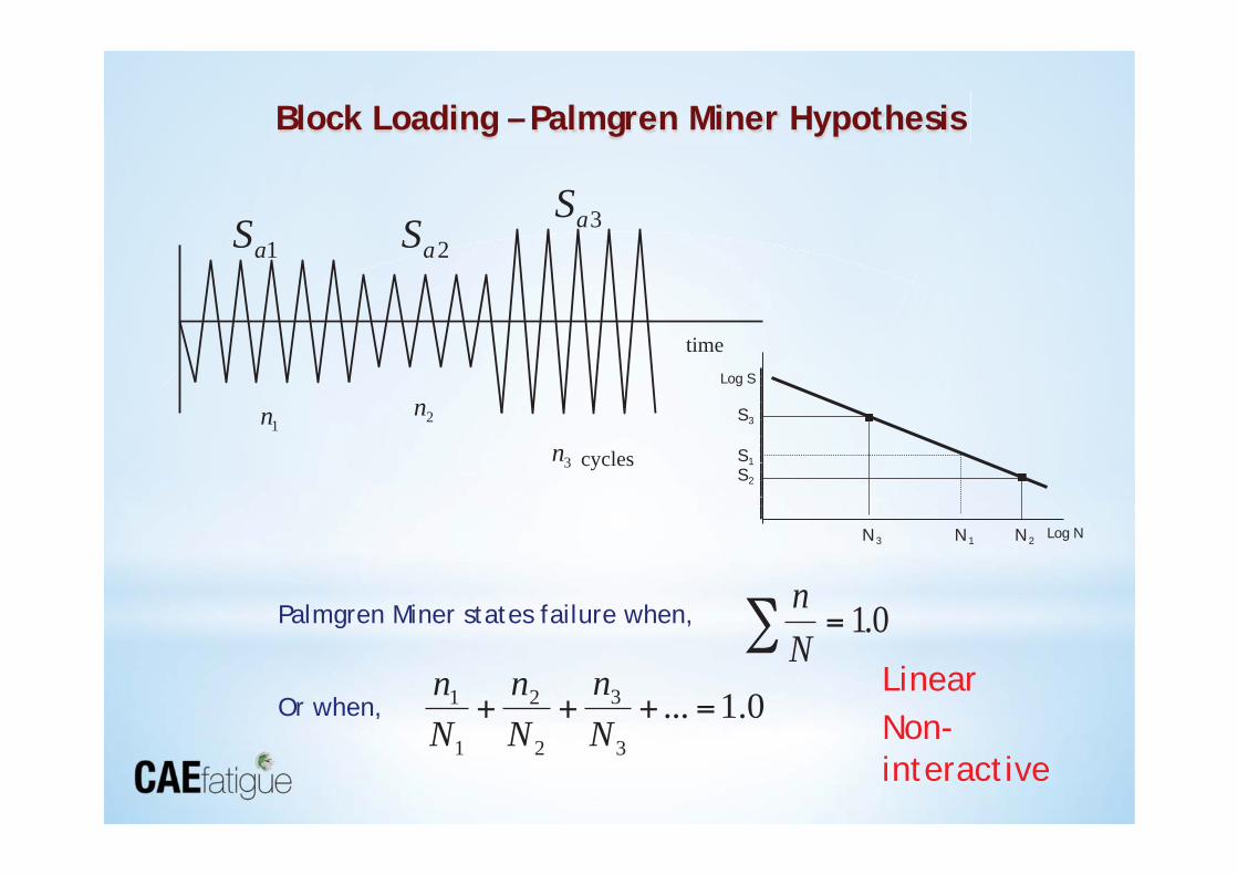
Block Loading – Palmgren Miner Hypothesis

Palmgren Miner states failure when,

Or when,

nN∑ = 10.

0.1...3

3

2

2

1

1 =+++Nn

Nn

Nn

time

1aS 2aS 3aS

1n 2n

3n cycles

Log S

Log N2 N

1 S

1 N3 N

2 S

3 S

Linear Non-interactive

S

N

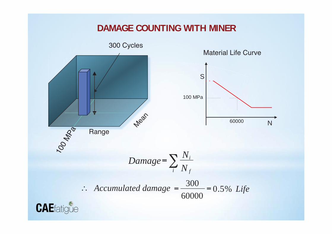
100 MPa

60000

Material Life Curve

LifeAccumulated damage %5.060000300 ==∴

Range

300 Cycles

∑=i f

i

NNDamage

DAMAGE COUNTING WITH MINER

1.45 x 10-3

300

500 1.21 x 10-3

250

2500 0.98 x 10-3

203

15000 0.76 x 10-3

157

120300 0.68 x 10-3

140

400000 0.60 x 10-3

124

1000000 0.54 x 10-3

112

3000000 0.45 x 10-3

93

5000000

Strain range recorded

Derived stress range (MPa)

Number of occurrences

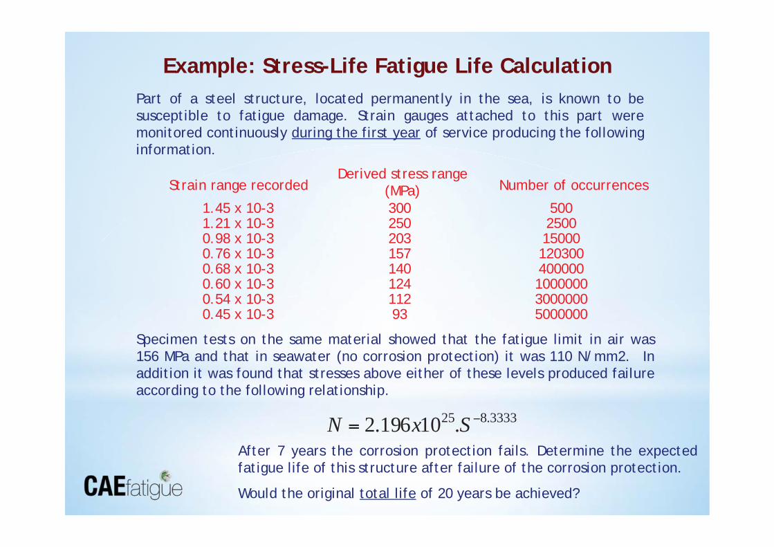
Part of a steel structure, located permanently in the sea, is known to be susceptible to fatigue damage. Strain gauges attached to this part were monitored continuously during the first year of service producing the following information.

Specimen tests on the same material showed that the fatigue limit in air was 156 MPa and that in seawater (no corrosion protection) it was 110 N/mm2. In addition it was found that stresses above either of these levels produced failure according to the following relationship.

3333.825.10196.2 −= SxNAfter 7 years the corrosion protection fails. Determine the expected fatigue life of this structure after failure of the corrosion protection.

Would the original total life of 20 years be achieved?

Example: Stress-Life Fatigue Life Calculation

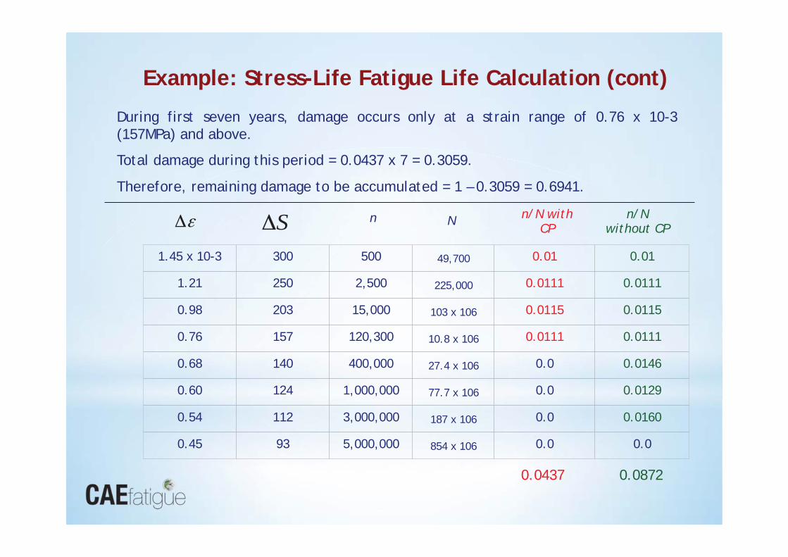
During first seven years, damage occurs only at a strain range of 0.76 x 10-3 (157MPa) and above.

Total damage during this period = 0.0437 x 7 = 0.3059.

Therefore, remaining damage to be accumulated = 1 – 0.3059 = 0.6941.

n

N

n/N with CP

n/N without CP

1.45 x 10-3

300

500

49,700 0.01

0.01

1.21

250

2,500

225,000 0.0111

0.0111

0.98

203

15,000

103 x 106 0.0115

0.0115

0.76

157

120,300

10.8 x 106 0.0111

0.0111

0.68

140

400,000

27.4 x 106 0.0

0.0146

0.60

124

1,000,000

77.7 x 106 0.0

0.0129

0.54

112

3,000,000

187 x 106 0.0

0.0160

0.45

93

5,000,000

854 x 106 0.0

0.0

SΔεΔ

Example: Stress-Life Fatigue Life Calculation (cont)

0.0437 0.0872

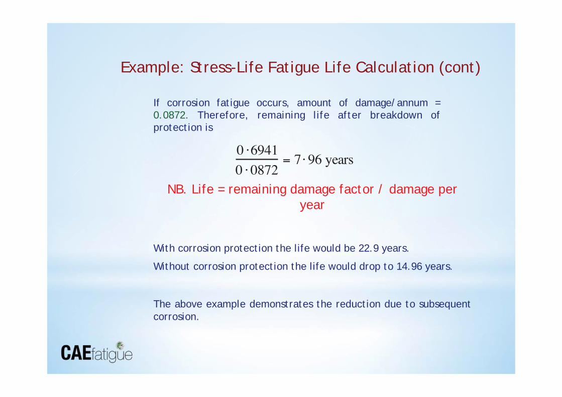
0 ⋅6941

0 ⋅ 0872= 7⋅ 96 years

If corrosion fatigue occurs, amount of damage/annum = 0.0872. Therefore, remaining life after breakdown of protection is

NB. Life = remaining damage factor / damage per year

With corrosion protection the life would be 22.9 years.

Without corrosion protection the life would drop to 14.96 years.

The above example demonstrates the reduction due to subsequent corrosion.

Example: Stress-Life Fatigue Life Calculation (cont)

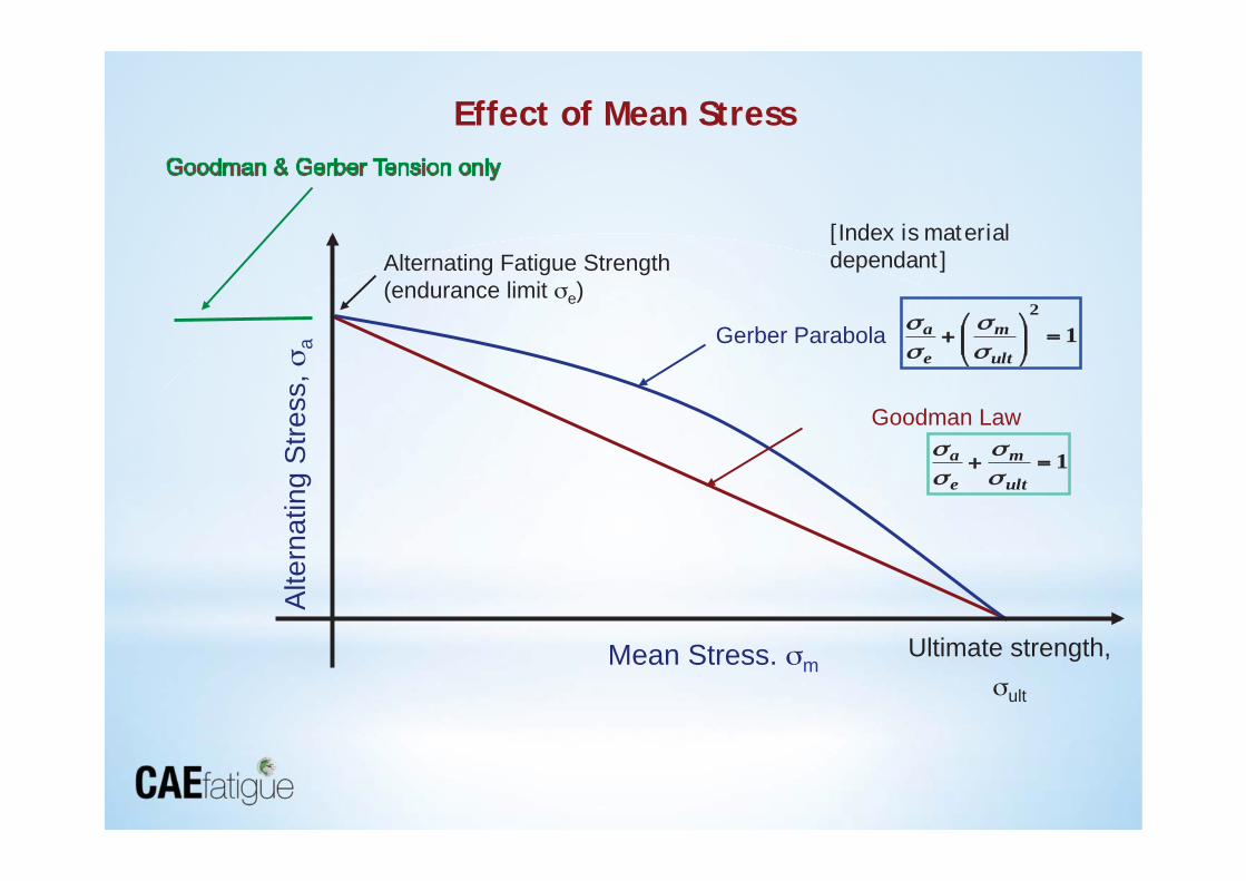
Effect of Mean Stress

Ultimate strength, σult

Alternating Fatigue Strength (endurance limit σe)

Mean Stress. σm

Alte

rnat

ing

Stre

ss, σ

a

Goodman Law 1=+

ult

m

e

aσσ

σσ

Gerber Parabola 12

=⎟⎟⎠

⎞⎜⎜⎝

⎛+

ult

m

e

aσσ

σσ

[Index is material dependant]

Correcting for the Effect of Mean Stress (Stress-Life Method)

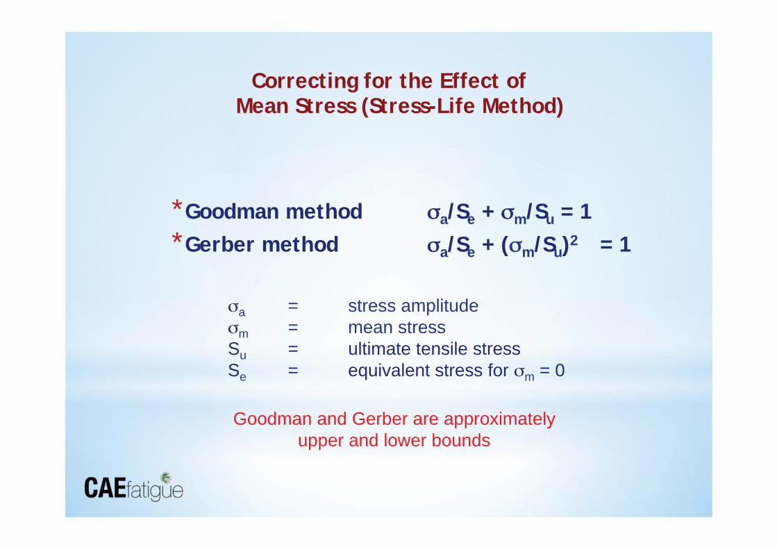
* Goodman method σσa/Se + σm/Su = 1 * Gerber method σa/Se + (σm/Su)2 = 1

Goodman and Gerber are approximately upper and lower bounds

σa = stress amplitude σm = mean stress Su = ultimate tensile stress Se = equivalent stress for σm = 0

Mean Stress Correction – Multiple S-N Curves

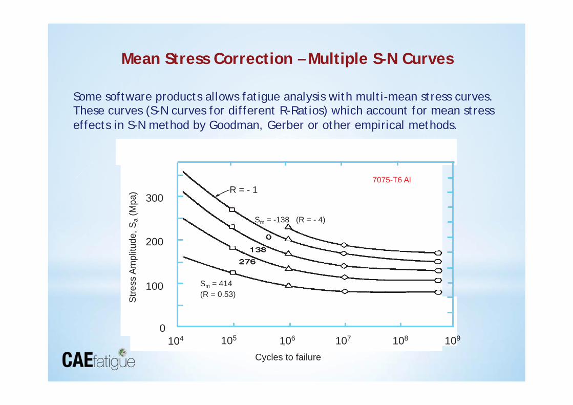
Some software products allows fatigue analysis with multi-mean stress curves. These curves (S-N curves for different R-Ratios) which account for mean stress effects in S-N method by Goodman, Gerber or other empirical methods.

104 105 106 107 108 109 0

100

200

300

Cycles to failure

Stre

ss A

mpl

itude

, Sa (

Mpa

) R = - 1

Sm = -138 (R = - 4)

Sm = 414 (R = 0.53)

7075-T6 Al

A component undergoes an operating cyclic stress with a maximum value of 759 MPa and a minimum value of 69 MPa. The component is made from a steel with an ultimate strength Su of 1035 MPa, an endurance limit Se (at 106) of 414 MPa and a fully reversed stress at 1000 cycles, S1000 of 759 MPa.

Plot a Goodman diagram with 2 constant life lines on it corresponding to 103 and 106 cycles. These must both go through Su on the zero mean stress amplitude (x) axis and the appropriate points on the stress amplitude (y) stress axis which are the endurance limit, Se, and S1000 values (see Figure below).

Example: Correcting For Mean Stress Effects

Sa=345 Sm=414

103

106

759

573

414

Su=1035

Altern

ating S

tress

S a (MP

a)

Mean Stress Sm (MPa)

.

S a=0 =

S 0

= 345MPa

= 414MPa

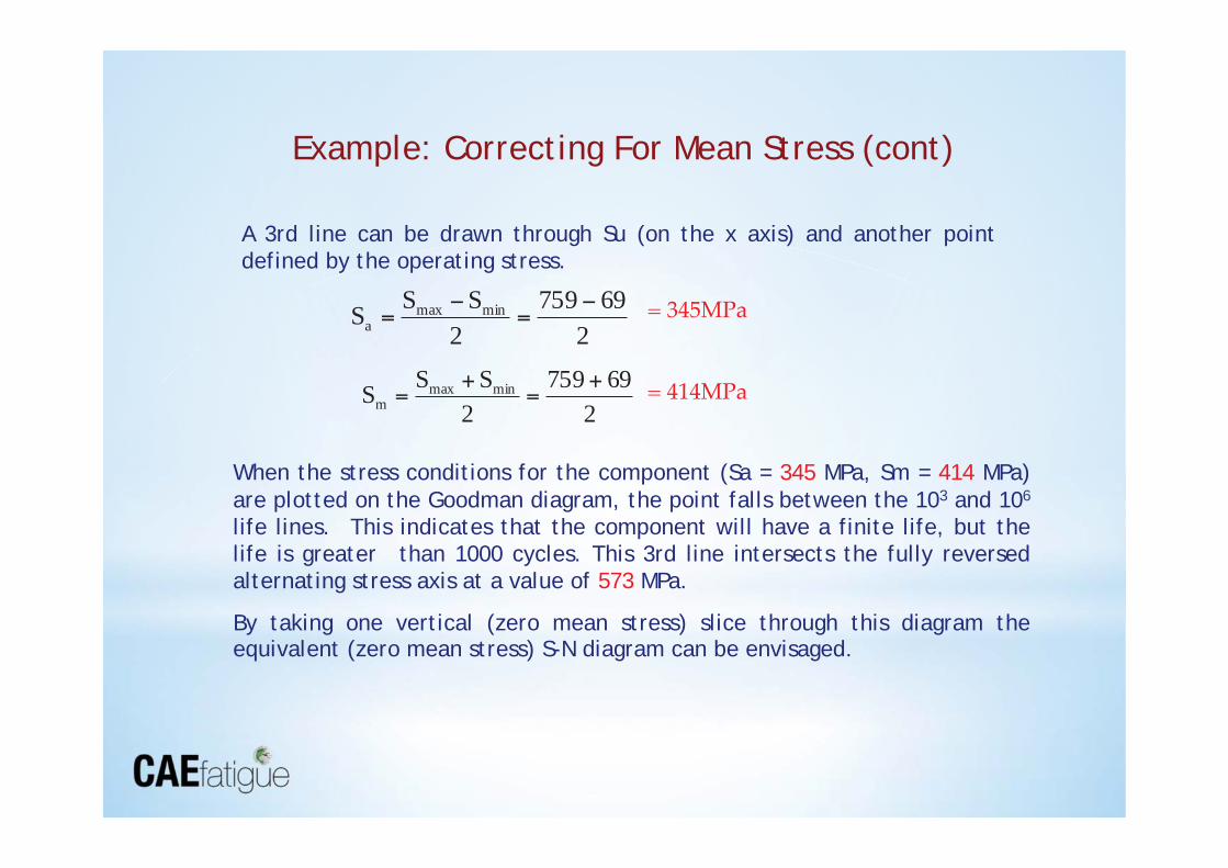
When the stress conditions for the component (Sa = 345 MPa, Sm = 414 MPa) are plotted on the Goodman diagram, the point falls between the 103 and 106 life lines. This indicates that the component will have a finite life, but the life is greater than 1000 cycles. This 3rd line intersects the fully reversed alternating stress axis at a value of 573 MPa.

By taking one vertical (zero mean stress) slice through this diagram the equivalent (zero mean stress) S-N diagram can be envisaged.

A 3rd line can be drawn through Su (on the x axis) and another point defined by the operating stress.

269759

2SSS minmax

a−

=−

=

269759

2SSS minmax

m+

=+

=

Example: Correcting For Mean Stress (cont)

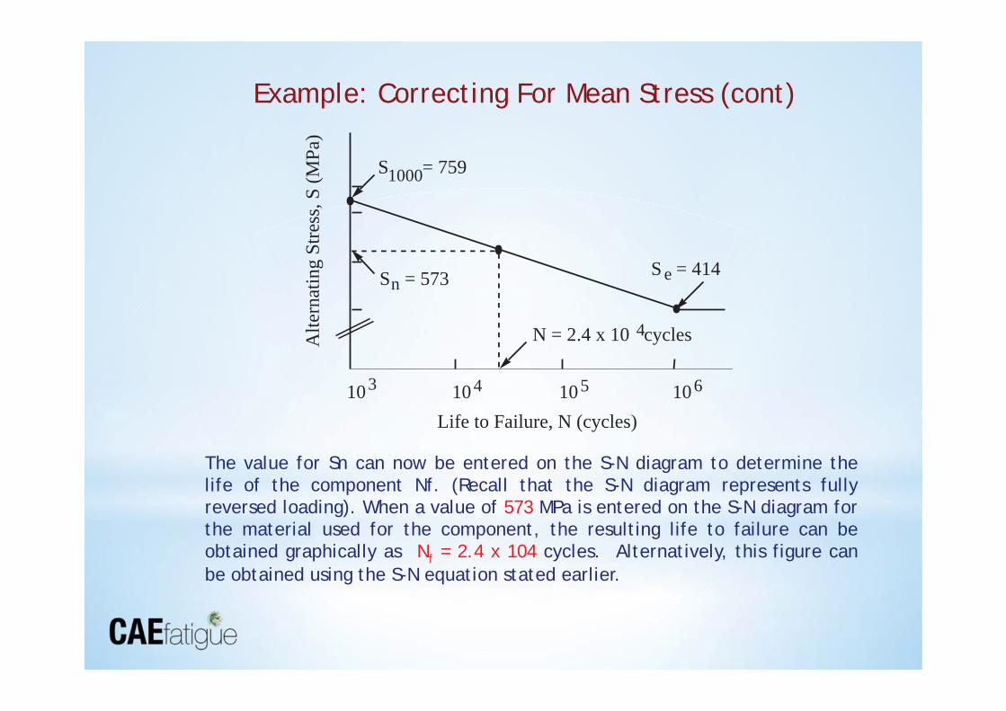
The value for Sn can now be entered on the S-N diagram to determine the life of the component Nf. (Recall that the S-N diagram represents fully reversed loading). When a value of 573 MPa is entered on the S-N diagram for the material used for the component, the resulting life to failure can be obtained graphically as Nf = 2.4 x 104 cycles. Alternatively, this figure can be obtained using the S-N equation stated earlier.

10 6 3 10 4 10 5 10

Alte

rnat

ing

Stre

ss, S

(MPa

)

Life to Failure, N (cycles)

S = 759 1000

S = 573 n S = 414 e

N = 2.4 x 10 cycles 4

Example: Correcting For Mean Stress (cont)

-200

-100

0

100

200

300

400

500

600

-2

-1.5

-1

-0.5

0

0.5

1

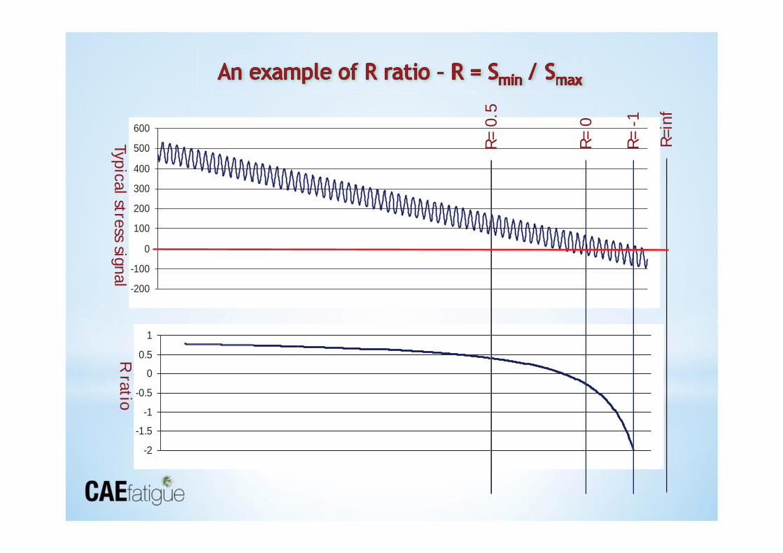
Typical stress signal R ratio

R=in

f

R= -

1

R= 0

R= 0

.5

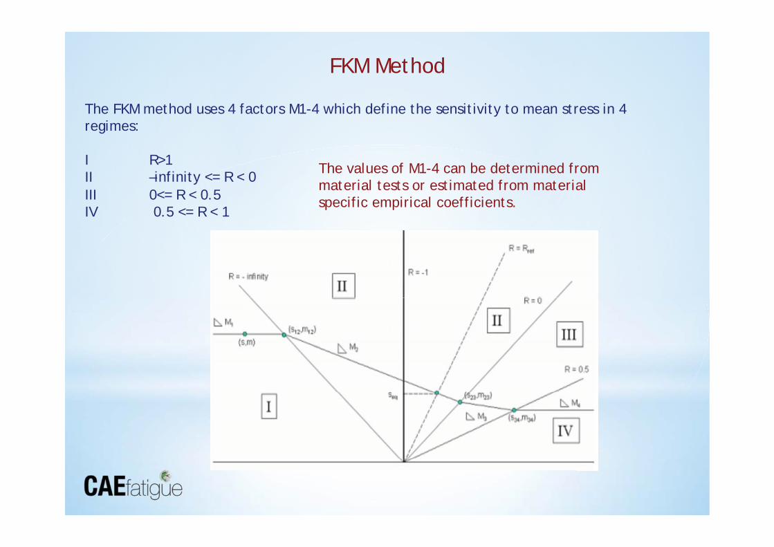
FKM Method

The FKM method uses 4 factors M1-4 which define the sensitivity to mean stress in 4 regimes: I R>1 II –infinity <= R < 0 III 0<= R < 0.5 IV 0.5 <= R < 1

The values of M1-4 can be determined from material tests or estimated from material specific empirical coefficients.

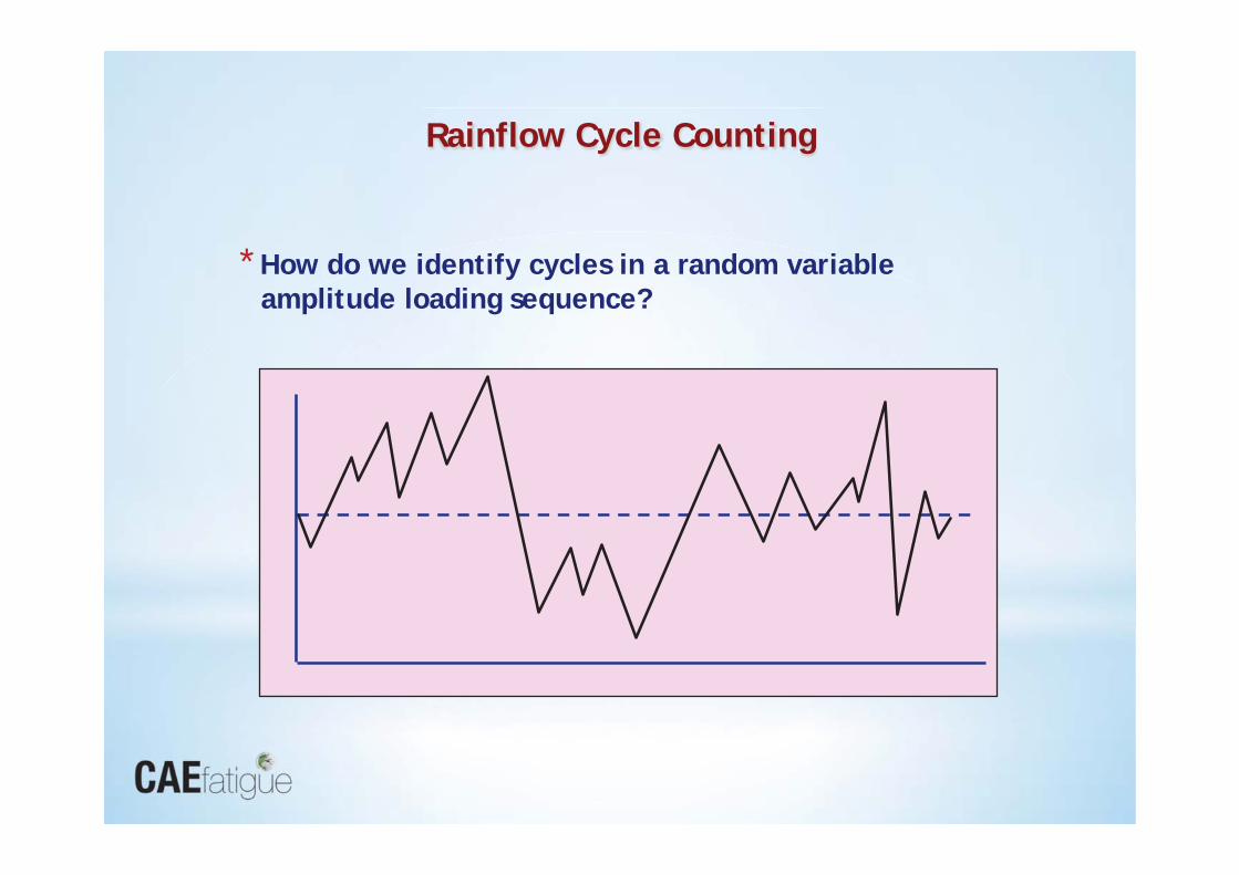
Rainflow Cycle Counting

* How do we identify cycles in a random variable amplitude loading sequence?

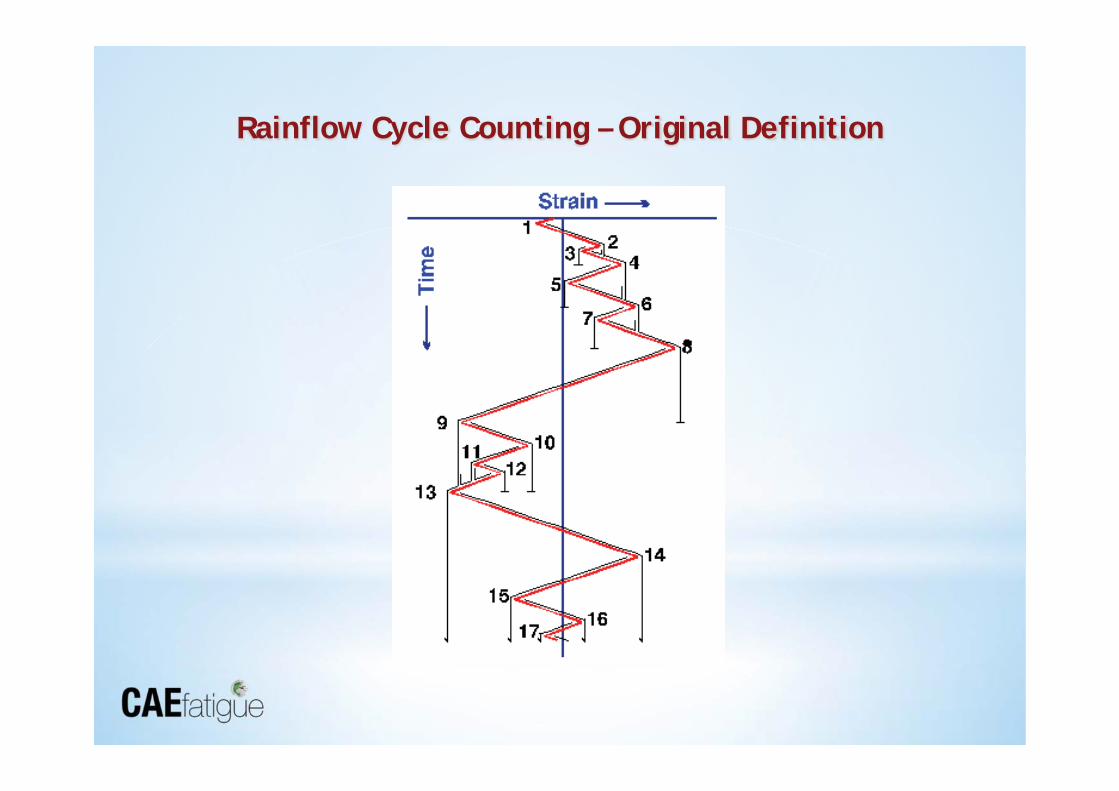
Rainflow Cycle Counting – Original Definition

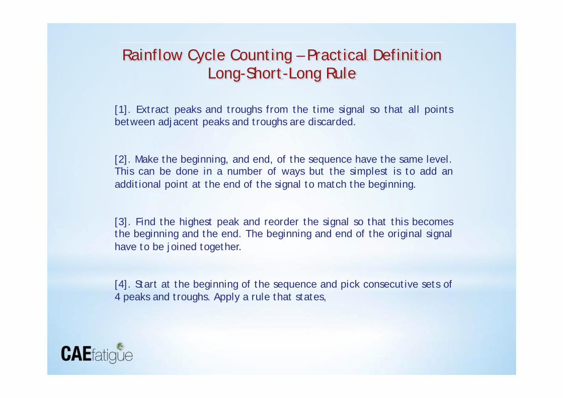
[1]. Extract peaks and troughs from the time signal so that all points between adjacent peaks and troughs are discarded.

[2]. Make the beginning, and end, of the sequence have the same level. This can be done in a number of ways but the simplest is to add an additional point at the end of the signal to match the beginning.

[3]. Find the highest peak and reorder the signal so that this becomes the beginning and the end. The beginning and end of the original signal have to be joined together.

[4]. Start at the beginning of the sequence and pick consecutive sets of 4 peaks and troughs. Apply a rule that states,

Rainflow Cycle Counting – Practical Definition Long-Short-Long Rule

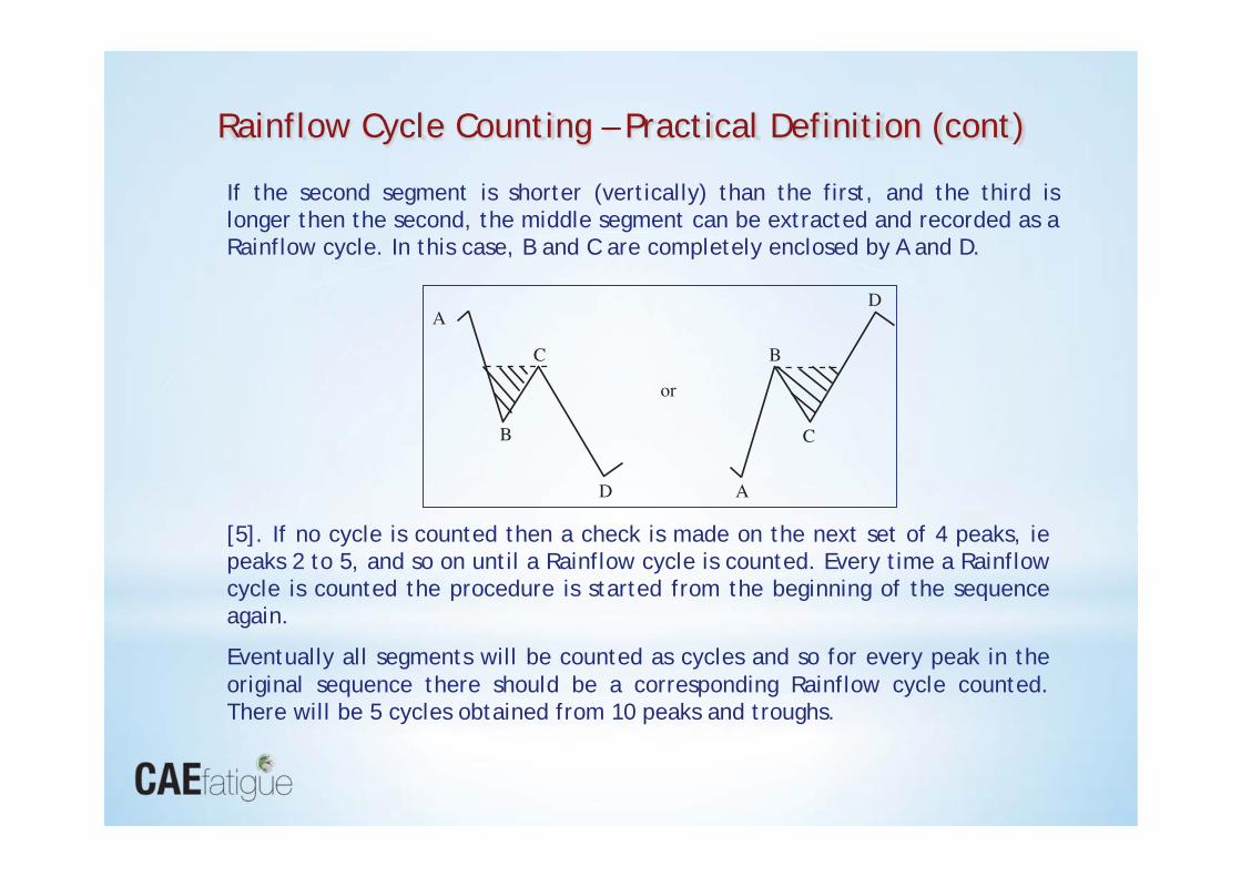
If the second segment is shorter (vertically) than the first, and the third is longer then the second, the middle segment can be extracted and recorded as a Rainflow cycle. In this case, B and C are completely enclosed by A and D.

[5]. If no cycle is counted then a check is made on the next set of 4 peaks, ie peaks 2 to 5, and so on until a Rainflow cycle is counted. Every time a Rainflow cycle is counted the procedure is started from the beginning of the sequence again.

Eventually all segments will be counted as cycles and so for every peak in the original sequence there should be a corresponding Rainflow cycle counted. There will be 5 cycles obtained from 10 peaks and troughs.

Rainflow Cycle Counting – Practical Definition (cont)

A

B C

D

or

A

B C

D

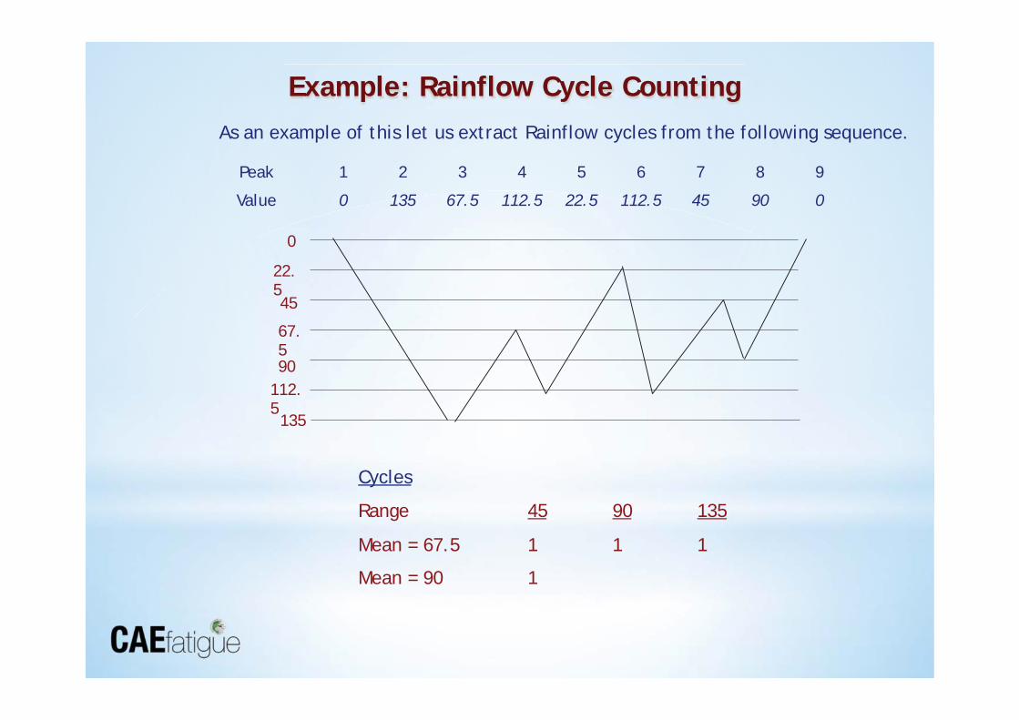
Peak

1

2

3

4

5

6

7

8

9 Value

0

135

67.5

112.5

22.5

112.5

45

90

0

Example: Rainflow Cycle Counting

Cycles

Range 45 90 135

Mean = 67.5 1 1 1

Mean = 90 1

0

22.5 45

67.5 90

112.5 135

As an example of this let us extract Rainflow cycles from the following sequence.

Variable Amplitude Loading

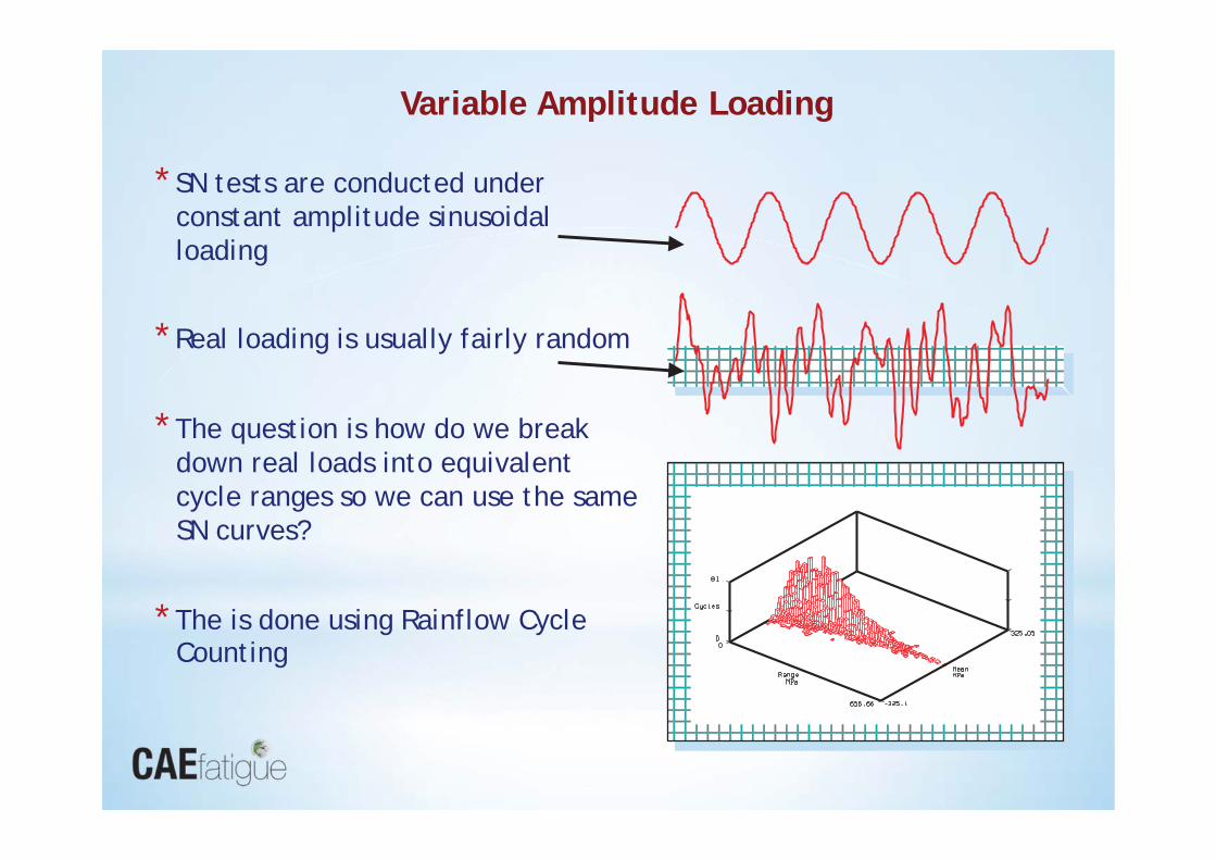
* SN tests are conducted under constant amplitude sinusoidal loading

* Real loading is usually fairly random

* The question is how do we break down real loads into equivalent cycle ranges so we can use the same SN curves?

* The is done using Rainflow Cycle Counting

mSKN =