An Intertemporal General Equilibrium Model of Asset PricesAuthor(s): John C. Cox, Jonathan E. Ingersoll, Jr., Stephen A. RossReviewed work(s):Source: Econometrica, Vol. 53, No. 2 (Mar., 1985), pp. 363-384Published by: The Econometric SocietyStable URL: http://www.jstor.org/stable/1911241 .Accessed: 03/02/2012 02:57

Your use of the JSTOR archive indicates your acceptance of the Terms & Conditions of Use, available at .http://www.jstor.org/page/info/about/policies/terms.jsp

JSTOR is a not-for-profit service that helps scholars, researchers, and students discover, use, and build upon a wide range ofcontent in a trusted digital archive. We use information technology and tools to increase productivity and facilitate new formsof scholarship. For more information about JSTOR, please contact support@jstor.org.

The Econometric Society is collaborating with JSTOR to digitize, preserve and extend access to Econometrica.

http://www.jstor.org

Econometrica, Vol. 53, No. 2 (March, 1985)

AN INTERTEMPORAL GENERAL EQUILIBRIUM MODEL OF ASSET PRICES'

BY JOHN C. COX, JONATHAN E. INGERSOLL, JR., AND STEPHEN A. Ross

This paper develops a continuous time general equilibrium model of a simple but complete economy and uses it to examine the behavior of asset prices. In this model, asset prices and their stochastic properties are determined endogenously. One principal result is a partial differential equation which asset prices must satisfy. The solution of this equation gives the equilibrium price of any asset in terms of the underlying real variables in the economy.

1. INTRODUCTION

IN THIS PAPER, we develop a general equilibrium asset pricing model for use in applied research. An important feature of the model is its integration of real and financial markets. Among other things, the model endogenously determines the stochastic process followed by the equilibrium price of any financial asset and shows how this process depends on the underlying real variables. The model is fully consistent with rational expectations and maximizing behavior on the part of all agents.

Our framework is general enough to include many of the fundamental forces affecting asset markets, yet it is tractable enough to be specialized easily to produce specific testable results. Furthermore, the model can be extended in a number of straightforward ways. Consequently, it is well suited to a wide variety of applications. For example, in a companion paper, Cox, Ingersoll, and Ross [7], we use the model to develop a theory of the term structure of interest rates.

Many studies have been concerned with various aspects of asset pricing under uncertainty. The most relevant to our work are the important papers on intertem- poral asset pricing by Merton [19] and Lucas [16]. Working in a continuous time framework, Merton derives a relationship among the equilibrium expected rates of return on assets. He shows that when investment opportunities are changing randomly over time this relationship will include effects which have no analogue in a static one period model. Lucas considers an economy with homogeneous individuals and a single consumption good which is produced by a number of processes. The random output of these processes is exogenously determined and perishable. Assets are defined as claims to all or a part of the output of a process, and the equilibrium determines the asset prices.

Our theory draws on some elements of both of these papers. Like Merton, we formulate our model in continuous time and make full use of the analytical tractability that this affords. The economic structure of our model is somewhat similar to that of Lucas. However, we include both endogenous production and

' This paper is an extended version of the first half of an earlier working paper titled "A Theory of the Term Structure of Interest Rates." We are grateful for the helpful comments and suggestions of many of our colleagues, both at our own institutions and others. This research was partially supported by the Dean Witter Foundation, the Center for Research in Security Prices, and the National Science Foundation.

363

364 J. C. COX, J. E. INGERSOLL, JR., AND S. A. ROSS

random technological change. Since we allow for randomly changing investment opportunities, the intertemporal effects noted by Merton apply to our model and play an important role in our results.

In independent work, Brock [4,5] and Prescott and Mehra [22] have also developed intertemporal models of asset pricing. The general approach of their papers is similar to ours, but the methods used and the issues addressed are quite different. Other related work includes papers by Breeden [3], Constantinides [6], Donaldson and Mehra [9], Huang [14], Richard and Sundaresan [24], Rubinstein [26], and Stapleton and Subrahmanyam [28].

Our paper is organized in the following way. In Section 2, we develop the model and characterize the equilibrium interest rate and equilibrium rates of return on assets. Section 3 presents our fundamental valuation equation and interprets its solution in a number of ways. Section 4 shows the relationship of our model to the Arrow-Debreu model and discusses the role of firms. In Section 5, we provide some concluding remarks and discuss several possible generalizations of our results.

2. AN EQUILIBRIUM VALUATION MODEL

This section will develop a model of general equilibrium in a simple economic setting. The following assumptions characterize our economy.

ASSUMPTION Al: There is a single physical good which may be allocated to consumption or investment. All values are expressed in terms of units of this good.

ASSUMPTION A2: Production possibilities consist of a set of n linear activities.2 The transformation of an investment of a vector -q of amounts of the good in the n production processes is governed by a system of stochastic differential equations of the form :3'4

(1) d77 (t) =Ia (x(Y, t) dt +In,G( Y, t) dw(t),

2 We consider a pure capital growth model by assuming that labor is unnecessary in production (or that there is a permanent labor surplus state). This provides a more streamlined setting for the issues which we wish to stress. There is no essential difficulty in expanding the analysis to include labor inputs and nonlinear technologies.

3 In describing the probabilistic structure of the economy, we will be implicitly referring to an underlying probability space (D, A, OP). Here n2 is a set, /3 is a cr-algebra of subsets of Q2, and !P is a probability measure on _. Let [t, t'] be a time interval and M be a separable complete metric space. By a stochastic process z, we mean a function from [t, t'] x Q2 into M such that z is measurable with respect to -03 and the cr-algebra of Borel subsets of M. We will take M to be R', n-dimensional Euclidean space. A stochastic process is said to be continuous if its possible realizations, or sample paths, are continuous with probability one. A real valued process w on [t, t'] is a Wiener process if: (i) w is a continuous process with independent increments, (ii) w(s) - w(t) has a normal distribution with mean zero and variance s - t. A process is an n-dimensional Wiener process if its components are independent one-dimensional Wiener processes.

4 Stochastic differential equations used in this paper are to be understood in the following way. Let x(t) be an m-dimensional stochastic process which satisfies the system of stochastic differential equations

dx = a(x, t) dt + B(x, t) dw(t),

ASSET PRICES

where w(t) is an (n + k) dimensional Wiener process in R"+k, Yis a k-dimensional vector of state variables whose movement will be described shortly, I, is an n x n diagonal matrix valuedfunction of r7 whose ith diagonal element is the ith component of 7r, a( Y, t) = [ai( Y, t)] is a bounded n-dimensional vector valued function of Y and t, and G( Y, t) = [gij( Y, t)] is a bounded n x (n + k) matrix valued function of Yand t. The covariance matrix ofphysical rates of return on the production processes, GG', is positive definite.5

System (1) specifies the growth of an initial investment when the output of each process is continually reinvested in that same process. It thus provides a complete description of the available production opportunities. It does not imply that individuals or firms will necessarily reinvest in this way. The production processes have stochastic constant returns to scale in the sense that the distribution of the rate of return on an investment in any process is independent of the scale of the investment.6

ASSUMPTION A3: The movement of the k-dimensional vector of state variables, Y, is determined by a system of stochastic differential equations of the form:

(2) dY(t) = ( Y, t) dt + S(Y, t) dw(t),

where a(x, t) is an m x 1 vector valued function and B(x, t) is an m x n matrix valued function, and w(t) is an n-dimensional Wiener process. A solution of this system with initial position x(t) is a solution of the system of integral equations

x(s)=x(t)4+ a(x(u), u) du++ B(x(u), u) dw(u),

where the latter integral is defined in the sense of Ito. We assume, in reference to (1), (2), and (3), that a and B are measurable on [t, t']xR " and

satisfy the following growth and Lipschitz conditions: (i) There exists a constant k] such that for all (x, s) in [t, t'] x Rm,

la(x, s)l kl(l + Ix) and IB(x, s)l kl(l + [x).

(ii) For any bounded Qc R'" there exists a constant k2, possibly depending on Q and s, such that for all x, y e Q and t s <- t',

la(x, s)- a(y, s)| < k2Ix y\,

IB(x, s)- B(y, s)l < k2jx-yl.

Detailed information on all of these topics can be found in Fleming and Rishel [10], Friedman [11], and Gihman and Skorohod [12].

5 When discussing stochastic differential equations as given in footnote 4, we will refer to a(x(t), t) as the vector of expected returns (or changes) of x and B(x(t), t)B'(x(t), t) as the covariance matrix of returns (or changes) of x. Similarly, if Ix is a diagonal matrix with the ith component of x as its ith diagonal element, then I-la is the vector of expected rates of return (or rates of change or percentage changes) of x and I,-BB'I-1 is the covariance matrix of rates of return (or rates of change or percentage changes) of x.

6 This formulation allows for quite general probabilistic behavior by the capital stock. However, since the stochastic differential equations are driven by Wiener processes, sudden discontinuous changes in the capital stock are precluded. Note that the incremental return on an investment in any production process can be negative, thus reflecting random physical depreciation.

365

366 J. C. COX, J. E. INGERSOLL, JR., AND S. A. ROSS

where ,(Y, t) [,i (Y, t)] is a k-dimensional vector and S(Y, t)=[sij(Y, t)] is a k x (n + k) dimensional matrix. The covariance matrix of changes in the state variables, SS', is nonnegative definite. We will assume that Y has no accessible boundaries. Note that (2) need not be a linear homogeneous system, and that both Y and the joint process (-q, Y) are Markov.

This framework includes both uncertain production and random technological change. The probability distribution of current output depends on the current level of the state variables Y, which are themselves changing randomly over time. The development of Y will thus determine the production opportunities which will be available to the economy in the future. In general, opportunities may worsen as well as improve.

Unless GS' is a null matrix, changes in the state variables will be contem- poraneously correlated with the incremental returns on the production processes. Indeed, when S is identically equal to G, they are perfectly correlated and the value of Y at any time will be completely determined by the previous returns on the production processes. Consequently, our description of technological change can easily represent situations in which the random shocks to any individual production process are correlated over time.7

Y may also include state variables which do not affect production opportunities but are nevertheless of interest to individuals. We postpone further discussion of these variables until a suitable context is developed later in the paper.

ASSUMPTION A4: There is free entry to all production processes. Individuals can invest in physical production indirectly through firms or directly, in effect creating their own firms. We will adopt the second interpretation, with some remarks about the first. Individuals and firms are competitive and act as price takers in all markets.

ASSUMPTION A5: There is a marketfor instantaneous borrowing and lending at an interest rate r. The market clearing rate, as a function of underlying variables, is determined as part of the competitive equilibrium of the economy.

ASSUMPTION A6: There are marketsfor a variety of contingent claims to amounts of the good. These are securities which are issued and purchased by individuals and firms. The specification of each claim includes a full description of all payoffs which may be received from that claim. These payoffs may depend on the values of the state variables and on aggregate wealth. The values of the claims will in general depend on all variables necessary to describe the state of the economy. We can write the stochastic differential equation governing the movement of the value of claim i, F, as

(3) dF' = (F',8i - 5i) dt + F'hi dw (t)

7 As a simple example, suppose k = n, a = - Y, u = - Y, and S = G, where G is a constant diagonal matrix. Then Y is an n-dimensional first-order autoregressive process and (1) can be rewritten as di7(t) = In dY(t).

ASSET PRICES 367

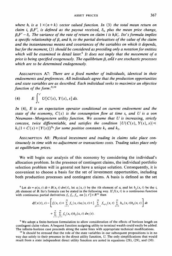
where hi is a 1 x (n + k) vector valued function. In (3) the total mean return on claim i, i3iF', is defined as the payout received, 8i, plus the mean price change, ,fiF' - 8i. The variance of the rate of return on claim i is hih'. Ito's formula implies a specific relationship of f3i and hi to the partial derivatives of the value of the claim and the instantaneous means and covariances of the variables on which it depends, butfor the moment, (3) should be considered as providing only a notationfor entities which will be examined in detail later.8 It does not imply that the movement of a price is being specified exogenously. The equilibrium fi antd r are stochastic processes which are to be determined endogenously.

ASSUMPTION A7: There are a fixed number of individuals, identical in their endowments and preferences. All individuals agree that the production opportunities and state variables are as described. Each individual seeks to maximize an objective function of the form :9 'O

rt'

(4) E U[C(s), Y(s), s] ds. t

In (4), E is an expectation operator conditional on current endowment and the state of the economy, C(s) is the consumption flow at time s, and U is a von Neumann-Morgenstern utility function. We assume that U is increasing, strictly concave, twice differentiable, and satisfies the condition I U(C(s), Y(s), s)I k1(I + C(s) + I Y(s)l)k2 for some positive constants k1 and k2.

ASSUMPTION A8: Physical investment and trading in claims take place con- tinuously in time with no adjustment or transactions costs. Trading takes place only at equilibrium prices.

We will begin our analysis of this economy by considering the individual's allocation problem. In the presence of contingent claims, the individual portfolio selection problem will in general not have a unique solution. Consequently, it is convenient to choose a basis for the set of investment opportunities, including both production processes and contingent claims. A basis is defined as the set

8 Let dx== a(x, t) dt+B(x, t) dw(t), let a,(x, t) be the ith element of a, and let bi,(x, t) be the i, jth element of B. Ito's formula can be stated in the following way. If f(x, t) is a continuous function with continuous partial derivatives f,, fX, fXX on [t, t'] x R m then

m tn mn df(x (t), t)= f (x t)+ Ef-(x f fxk x,(x, t) dt

j,k=1 i=

Ft m + E E fx (x, t)b,,(x, t) dw,(t).

9 We adopt a finite-horizon formulation to allow consideration of the effects of horizon length on contingent claim values. A bequest function assigning utility to terminal wealth could easily be added. The infinite-horizon case proceeds along the same lines with appropriate technical modifications.

'1 It should be stressed that the role of the state variables in our subsequent propositions is in no way due solely to their presence in the direct utility function, U. The only simplifications that would result from a state independent direct utility function are noted in equations (28), (29), and (30).

368 J. C. COX, J. E. INGERSOLL, JR., AND S. A. ROSS

of production processes and a set of contingent claims, with row vectors hi, as in (3), forming the matrix H, such that for any other contingent claim j, hj can be written as a linear combination of the rows of G and H. Equation (3) will now be interpreted as referring to the claims in the basis. The explicit construction of the basis over time is not of importance as long as its dimension remains unchanged, which we assume to be the case. Any creation or expiration of contingent claims which causes a change in the dimension of the basis will cause a change in the hedging opportunities available to an individual. For simplicity we assume that the basis consists of the n production activities and k contingent claims.

It is sufficient for both individual choice and equilibrium valuation to determine the unique allocation resulting when the opportunity set is restricted to the basis. Any allocation involving nonbasis claims could be replicated by a controlled portfolio of claims in the basis. " Since any of these choices would give the individual the same portfolio behavior over time and the same consumption path, he would be indifferent among them. In this scheme of things there is no reason for nonbasis contingent claims to exist, but there is no reason for them not to exist either, and we may assume that in general there will be an infinite number of them, each of which must be consistently priced in equilibrium.'2

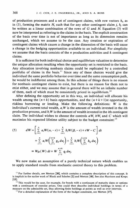
After defining the opportunity set in this way, an individual will allocate his wealth among the (n + k) basis opportunities, and the (n + k+ 1)st opportunity, riskless borrowing or lending. Make the following definitions: W is the individual's current total wealth, ai W is the amount of wealth invested in the ith production process, and bi W is the amount of wealth invested in the ith contingent claim. The individual wishes to choose the controls aW, bW, and C which will maximize his expected lifetime utility subject to the budget constraint:'3

n ~~~~k (5) dW= aiW(axi-r)+ biW(,6i-r)+rW-C dt

n n+k k /n+k

+ E aiW E gijdwj +E bi W E hi3dw) i=l j=l - j=l

n+k

-Wplk(W) dt+ W E q1dw>. j=l

We now make an assumption of a purely technical nature which enables us to apply standard results from stochastic control theory to this problem.

l For further details, see Merton [20], which contains a complete description of this concept. It is implicit in the earlier work of Black and Scholes [2] and Merton [18]. See also Harrison and Kreps [13].

12 This would be the case, for example, for bonds with a continuum of maturity dates or options with a continuum of exercise prices. One could then describe individual holdings in terms of a measure on the admissible set, thus allowing finite holdings at points as well as over intervals.

13 For a detailed explanation of the form of the budget constraint, see Merton [17].

ASSET PRICES 369

ASSUMPTION A9: In maximizing (4), the individual limits his attention to a class of admissible feedback controls, V. An admissible feedback control, v, is a Borel measurablefunction on [t, t') x R n+k+ 1 satisfying the growth and Lipschitz conditions given in footnote 4. Furthermore, admissible disequilibrium ,B and r are bounded and satisfy the Lipschitz conditions given in footnote 4.

Measurability implies the natural restriction that the control chosen at any time must depend only on information available at that time.

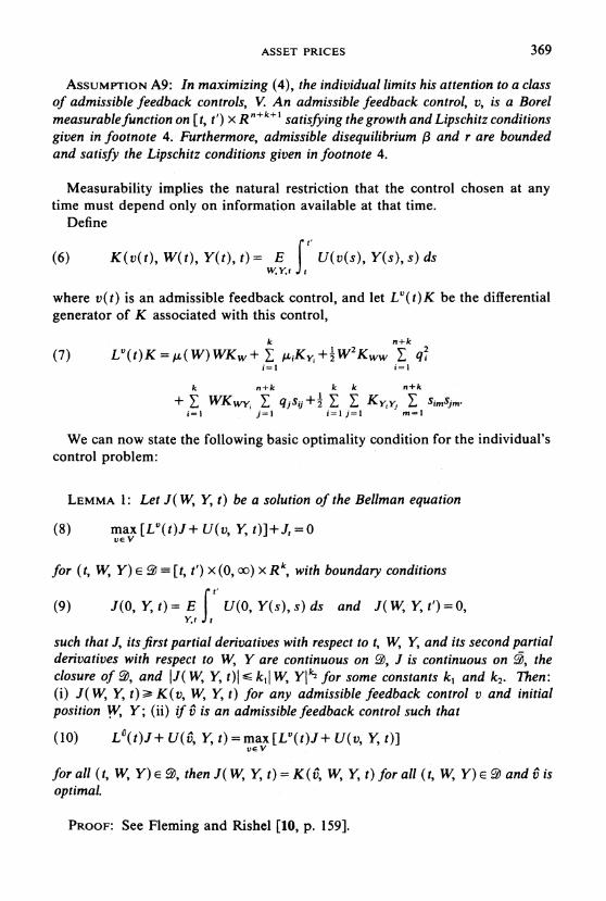
Define

(6) K(v(t), W(t), Y(t), t)= E j U(v(s), Y(s), s) ds W,Y,t t

where v(t) is an admissible feedback control, and let LV(t)K be the differential generator of K associated with this control,

k n+k

(7) Lv (t) K -,( W) WKw + a ,iKy, + 1W2 Kww q2 i= ti=1

k n+k k k n+k

+ E WKy , qjsij+ E E K y, y il j=1 i=l j=1 m I

We can now state the following basic optimality condition for the individual's control problem:

LEMMA 1: Let J(W, Y, t) be a solution of the Bellman equation

(8) max [LV(t)J + U(v, Y, t)] + Jt = 0

for (t, W, Y) e 9- [t, t') x (0, cc) x Rk, with boundary conditions t,

(9) J(O, Y, t) = E U(O, Y(s),s) ds and J(W, Y, t')=O, Y, t t

such that J, its first partial derivatives with respect to t, W, Y, and its second partial derivatives with respect to W, Y are continuous on !, J is continuous on 2, the closure of 2, and IJ( W, Y, t)j - k1l w, YIk2 for some constants k, and k2. Then: (i) J( W, Y, t) > K(v, W, Y, t) for any admissible feedback control v and initial position W, Y; (ii) if v is an admissible feedback control such that

(10) L6(t)J + U(v Y, t) =max [Lv(t)J + U(v, Y, t)] ve V

for all (t, W, Y)E2, thenJ( W, Y,t)-K(v, W, Y,t) for all (t, W, Y)E:iiandVis optimal.

PROOF: See Fleming and Rishel [10, p. 159].

370 J. C. COX, J. E. INGERSOLL, JR., AND S. A. ROSS

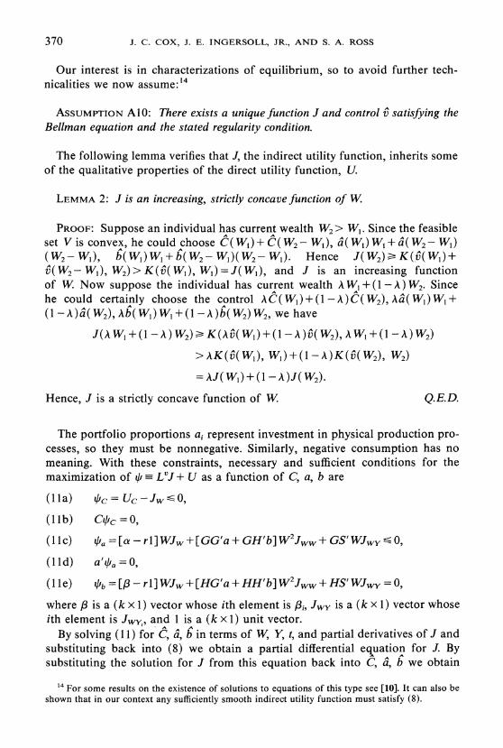
Our interest is in characterizations of equilibrium, so to avoid further tech- nicalities we now assume:"4

ASSUMPTION AIO: There exists a uniquefunction J and control v satisfying the Bellman equation and the stated regularity condition.

The following lemma verifies that J, the indirect utility function, inherits some of the qualitative properties of the direct utility function, U.

LEMMA 2: J is an increasing, strictly concave function of W.

PROOF: Suppose an individual has current wealth W2> W,. Since the feasible set V is convex, he could choose C(WD) + C(W2 - WI), a(W1)W1+a(W2- Wa) (W2- W1), b(W1) W, + b(W2- W,)(W2- WI). Hence J(W2) K (v(W)+ v( W2- W, W2)>K(v( W), WI) = J(W1), and J is an increasing function of W. Now suppose the individual has current wealth A W, + (1 - A) W2. Since he could certainly choose the control AC(W,)+(1-A)C(W2) Aa(W,)W,+ (1-A )(W2), Ab(W)W+(i- A)b(W2)W2 vwe have

J(AW,+(1 -A)W2) K(Av(W +(i-A)v(W2) AW1+(i-A)W2)

> AK(v(, WI) + (1- A)K(v( 2) 2)

= AJ(W,) + (I -A)J(W2).

Hence, J is a strictly concave function of W. Q.E.D.

The portfolio proportions ai represent investment in physical production pro- cesses, so they must be nonnegative. Similarly, negative consumption has no meaning. With these constraints, necessary and sufficient conditions for the maximization of qr LVJ + U as a function of C, a, b are

(I la) qc = Uc - Jw _< 09

(lIlb) CqcI=O0

(l IC) Oa= [a- -rl] WJw +[GG'a + GH'b] W2Jw+GS'WJwy0,

(lId) a'qla= 0

(l I e) qfb = [/ - r I] WJw + [HG'a + HH'b] W2J + HS WJWy 0,

where ,3 is a (k x 1) vector whose ith element is ,i, JWY is a (k x 1) vector whose ith element is JWY and 1 is a (k x 1) unit vector.

By solving ( 11) for C, a. b in terms of W, Y, t, and partial derivatives of J and substituting back into (8) we obtain a partial differential e%uation for J. By substituting the solution for J from this equation back into C, a b we obtain

14 For some results on the existence of solutions to equations of this type see [10]. It can also be shown that in our context any sufficiently smooth indirect utility function must satisfy (8).

ASSET PRICES 371

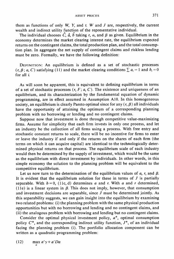
them as functions of only W, Y, and t. W and J are, respectively, the current wealth and indirect utility function of the representative individual.

The individual chooses C, a, b taking r, a, and ,B as given. Equilibrium in the economy determines the market clearing interest rate, the equilibrium expected returns on the contingent claims, the total production plan, and the total consump- tion plan. In aggregate the net supply of contingent claims and riskless lending must be zero. Formally, we have the following definition:

DEFINITION: An equilibrium is defined as a set of stochastic processes (r, ,8; a, C) satisfying ( 11) and the market clearing conditions E ai = 1 and bi =0 for all i.

As will soon be apparent, this is equivalent to defining equilibrium in terms of a set of stochastic processes (r, F; a, C). The existence and uniqueness of an equilibrium, and its characterization by the fundamental equation of dynamic programming, are in effect assumed in Assumption AIO. In this homogeneous society, an equilibrium is clearly Pareto optimal since for any (r, /) all individuals have the opportunity of attaining the optimum of a corresponding planning problem with no borrowing or lending and no contingent claims.

Suppose now that investment is done through competitive value-maximizing firms. Assume for simplicity that each firm invests in only one process, and let an industry be the collection of all firms using a process. With free entry and stochastic constant returns to scale, there will be no incentive for firms to enter or leave the industry if and only if the returns on the shares of each firm (the terms on which it can acquire capital) are identical to the technologically deter- mined physical returns on that process. The equilibrium scale of each industry would then be determined by the supply of investment, which would be the same as the equilibrium with direct investment by individuals. In other words, in this simple economy the solution to the planning problem will be equivalent to the competitive equilibrium.

Let us now turn to the determination of the equilibrium values of a, r, and X3. It is evident that the equilibrium solution for these in terms of J is partially separable. With b =0, (11 c, d) determines a and r. With a and r determined, ( lle) is a linear system in /3. This does not imply, however, that consumption and investment decisions are separable, since J must be determined jointly. As this separability suggests, we can gain insight into the equilibrium by examining two related problems: (i) the planning problem with the same physical production opportunities but with no borrowing and lending and no contingent claims, and (ii) the analogous problem with borrowing and lending but no contingent claims.

Consider the optimal physical investment policy, a* , optimal consumption policy C*, and the corresponding indirect utility function, J*, of an individual facing the planning problem (i). The portfolio allocation component can be written as a quadratic programming problem:

(12) max a'y+a'Da a1

372 J. C. COX, J. E. INGERSOLL, JR., AND S. A. ROSS

subject to:

a'l = 1,

a - 0,

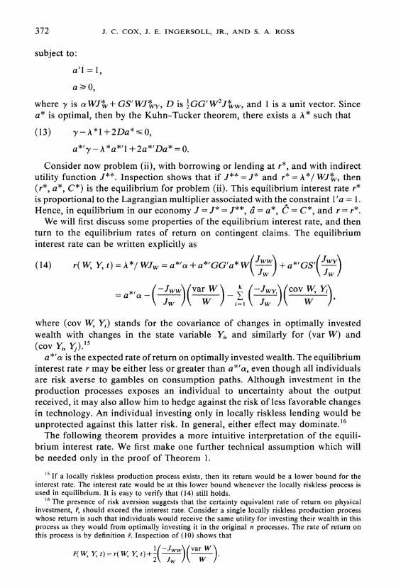
where y is a WJ* + GS'WJ* , D is 'GG' W2J* w, and 1 is a unit vector. Since a is optimal, then by the Kuhn-Tucker theorem, there exists a A* such that

(13) y - A*1 +2Da* O,

a*ly -A *a*'l + 2a*'Da* = O.

Consider now problem (ii), with borrowing or lending at r*, and with indirect utility function J**. Inspection shows that if J** = J* and r* = A*/ WJ*,, then (r*, a*, C*) is the equilibrium for problem (ii). This equilibrium interest rate r* is proportional to the Lagrangian multiplier associated with the constraint 1'a = 1.

*A= *A Hence, in equilibrium in our economy J = = J**, a = a C = C*, and r = r*. We will first discuss some properties of the equilibrium interest rate, and then

turn to the equilibrium rates of return on contingent claims. The equilibrium interest rate can be written explicitly as

(14) r( W, Y, t) = A*/ WJw = a*'a + a*'GG'a* W(Jw) + a*'GS'Q p-)

a (Jw )(aW ) i=1 (-Jw )(c W )

where (cov W, Yi) stands for the covariance of changes in optimally invested wealth with changes in the state variable Yi, and similarly for (var W) and (cov Yi, Y).1

a *l'a is the expected rate of return on optimally invested wealth. The equilibrium interest rate r may be either less or greater than a*'a, even though all individuals are risk averse to gambles on consumption paths. Although investment in the production processes exposes an individual to uncertainty about the output received, it may also allow him to hedge against the risk of less favorable changes in technology. An individual investing only in locally riskless lending would be unprotected against this latter risk. In general, either effect may dominate.16

The following theorem provides a more intuitive interpretation of the equili- brium interest rate. We first make one further technical assumption which will be needed only in the proof of Theorem 1.

15 If a locally riskless production process exists, then its return would be a lower bound for the interest rate. The interest rate would be at this lower bound whenever the locally riskless process is used in equilibrium. It is easy to verify that (14) still holds.

16 The presence of risk aversion suggests that the certainty equivalent rate of return on physical investment, F, should exceed the interest rate. Consider a single locally riskless, production process whose return is such that individuals would receive the same utility for investing their wealth in this process as they would from optimally investing it in the original n processes. The rate of return on this process is by definition F. Inspection of (10) shows that

F(W, Y,t)=r( W,Yt)+ Jw )( W

ASSET PRICES 373

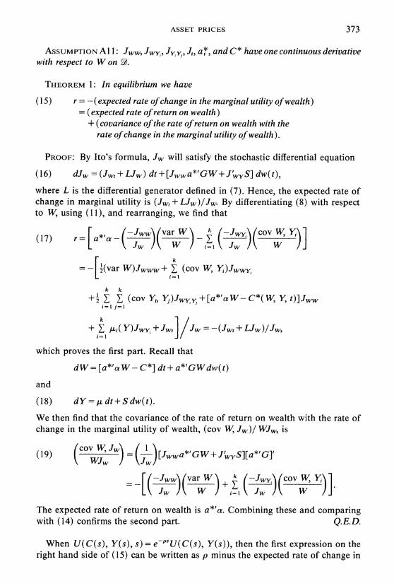
ASSUMPTION A 1: Jww, Jwy, JY,YJ, J, a*, and C * have one continuous derivative with respect to W on ?2.

THEOREM 1: In equilibrium we have

(15) r = -( expected rate of change in the marginal utility of wealth) = (expected rate of return on wealth)

+ (covariance of the rate of return on wealth with the rate of change in the marginal utility of wealth).

PROOF: By Ito's formula, Jw will satisfy the stochastic differential equation

( 16) dJw =(Jwt +LJw) dt +[Jwwa*'GW+J JWS] dw(t),

where L is the differential generator defined in (7). Hence, the expected rate of change in marginal utility is (Jwt + LJw)/Jw. By differentiating (8) with respect to W, using (11), and rearranging, we find that

(17) r= [a*a( Jww)(var W)_ ( Jw,)(cov W YE)]

k

= (var W)Jwww+ E (cov W, Yi)JWWY, i=l

k k

+ l E (cov Yi, Yj)Jwy,y+[a*'taW-C*( W, Y, t)]Jww i=l j=l

k 1 + E Hi,(Y)Jwy + Jwt I w = -(Jwt + LJW)/fw,

ji=lI

which proves the first part. Recall that

dW= [a*'a W - C*] dt+ a*'GWdw(t)

and

(18) dY= ,t dt+ Sdw(t).

We then find that the covariance of the rate of return on wealth with the rate of change in the marginal utility of wealth, (cov W, Jw)/ WJw, is

(19) (cov WJw) _ ( )[Jwwa*tGW+JwyS][a*tG]t

[(Jww) (var W ) ( Jwv) W Y)]

The expected rate of return on wealth is a*'a. Combining these and comparing with (14) confirms the second part. Q.E.D.

When U(C(s), Y(s), s)- e-PSU(C(s), Y(s)), then the first expression on the right hand side of (15) can be written as p minus the expected rate of change in

J. C. COX, J. E. INGERSOLL, JR., AND S. A. ROSS

the undiscounted marginal utility of wealth. These interpretations of course reduce to standard results when there is no uncertainty.

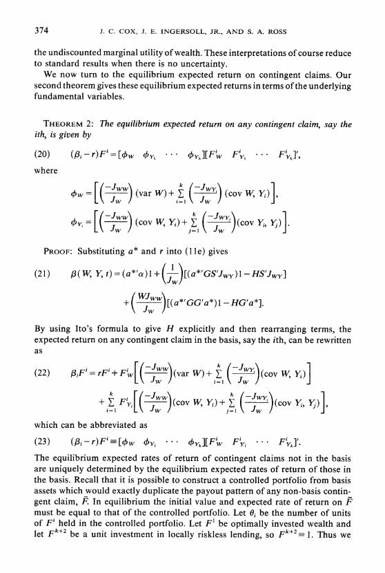
We now turn to the equilibrium expected return on contingent claims. Our second theorem gives these equilibrium expected returns in terms of the underlying fundamental variables.

THEOREM 2: The equilibrium expected return on any contingent claim, say the ith, is given by

(20) (i - r)F'i= [kw (y, ... * yk][FW Fy ... Fyk],

where

-Jww (vaW)+ Jw ] -w = (var W)+ IWY(cov W, Yi) _ Jw »i=l Jw

(by,= -(> ) =(cov W, Yi) + ( )(cov Yi, Yj) Jw j=l Jw

PROOF: Substituting a* and r into ( le) gives

(21) ( W, Y, t) = (a*'a) + (J )[(a*'GS'Jwy)l-HS'Jwy] WJww

+(JWJW )(a*'GG'a*)l -HG'a*]. Jw

By using Ito's formula to give H explicitly and then rearranging terms, the expected return on any contingent claim in the basis, say the ith, can be rewritten as

(22) F'= rF+Fw ( (varW)+ ( (cov W, Yi) k Jw =1 JwI

+ E FY ( )(c(cov W, YYj) i=l Jw j=l Jw

which can be abbreviated as

(23) (P3-r)F' -[w y, ... *

4>k][Fw FY, ' . Fk]'.

The equilibrium expected rates of return of contingent claims not in the basis are uniquely determined by the equilibrium expected rates of return of those in the basis. Recall that it is possible to construct a controlled portfolio from basis assets which would exactly duplicate the payout pattern of any non-basis contin- gent claim, F. In equilibrium the initial value and expected rate of return on F must be equal to that of the controlled portfolio. Let 0i be the number of units of F' held in the controlled portfolio. Let F' be optimally invested wealth and let Fk+2 be a unit investment in locally riskless lending, so Fk+2 = 1. Thus we

374

ASSET PRICES

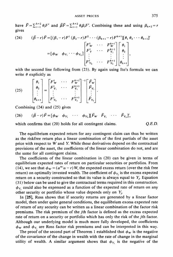
- k+2 k+2 have F=ik, 1j0iFi and 8F=F,j= O2ipF'. Combining these and using Pk+2=r

gives

(24) (+- r)F = [(,- r)F' (f,2-r)F2 ' . . ( ik+l- r)Fk+l][0I 02 ' ' 0k+l]'

FyW ... FkW+I 02

Fl F i;,k+' FYk ... FYk' k+I

with the second line following from (23). By again using Ito's formula we can write 0 explicitly as

Il ' kip+l'-' - oI FlW * - F Fw 02 F . FYI' '4

(25) 02 Y F F

k+1 FYk * * FkY' Fyk

Combining (24) and (25) gives

(26) (3-r)F=[kw kY, ... vYk][Fw Fy, ... Fyk],

which confirms that (20) holds for all contingent claims. Q.E.D.

The equilibrium expected return for any contingent claim can thus be written as the riskfree return plus a linear combination of the first partials of the asset price with respect to W and Y. While these derivatives depend on the contractual provisions of the asset, the coefficients of the linear combination do not, and are the same for all contingent claims.

The coefficients of the linear combination in (20) can be given in terms of equilibrium expected rates of return on particular securities or portfolios. From (14), we see that ckw = (a*'a - r) W, the expected excess return (over the risk free return) on optimally invested wealth. The coefficient of yj is the excess expected return on a security constructed so that its value is always equal to Yj. Equation (31) below can be used to give the contractual terms required in this construction. by could also be expressed as a function of the expected rate of return on any

other security or portfolio whose value depends only on Yj. In [25], Ross shows that if security returns are generated by a linear factor

model, then under quite general conditions, the equilibrium excess expected rate of return of any security can be written as a linear combination of the factor risk premiums. The risk premium of the jth factor is defined as the excess expected rate of return on a security or portfolio which has only the risk of the jth factor. Although our underlying model is much more fully developed, the coefficients kw and bY, are Ross factor risk premiums and can be interpreted in this way.

The proof of the second part of Theorem 1 established that >w is the negative of the covariance of the change in wealth with the rate of change in the marginal utility of wealth. A similar argument shows that cy, is the negative of the

375

376 J. C. COX, J. E. INGERSOLL, JR., AND S. A. ROSS

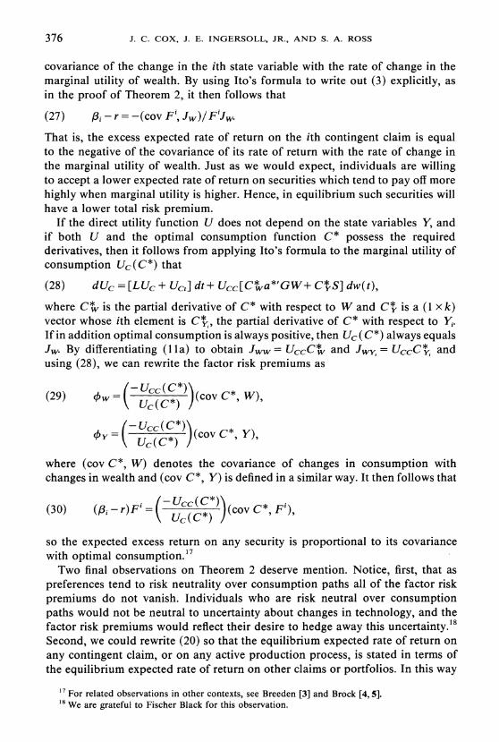
covariance of the change in the ith state variable with the rate of change in the marginal utility of wealth. By using Ito's formula to write out (3) explicitly, as in the proof of Theorem 2, it then follows that

(27) A, - r = -(cov Fi, Jw)/F'Jw.

That is, the excess expected rate of return on the ith contingent claim is equal to the negative of the covariance of its rate of return with the rate of change in the marginal utility of wealth. Just as we would expect, individuals are willing to accept a lower expected rate of return on securities which tend to pay off more highly when marginal utility is higher. Hence, in equilibrium such securities will have a lower total risk premium.

If the direct utility function U does not depend on the state variables Y, and if both U and the optimal consumption function C* possess the required derivatives, then it follows from applying Ito's formula to the marginal utility of consumption Uc(C*) that

(28) dUc = [LUc + Uct] dt+ Ucc[C* a*'GW+ C* S] dw(t),

where C* is the partial derivative of C* with respect to W and C* is a (1 x k) vector whose ith element is C*,, the partial derivative of C* with respect to Yi. If in addition optimal consumption is always positive, then Uc (C*) always equals

Jw. By differentiating ( lla) to obtain Jww = UcC* and JwyI = UccC* and using (28), we can rewrite the factor risk premiums as

(29) OW=-b:%c(j;)) (cov C*, W),

OY=( u (C*) )(cov C*, Y),

where (cov C*, W) denotes the covariance of changes in consumption with changes in wealth and (cov C*, Y) is defined in a similar way. It then follows that

(30) (/i - r)F = ( U (C))(cov C*, Fi),

so the expected excess return on any security is proportional to its covariance with optimal consumption.17

Two final observations on Theorem 2 deserve mention. Notice, first, that as preferences tend to risk neutrality over consumption paths all of the factor risk premiums do not vanish. Individuals who are risk neutral over consumption paths would not be neutral to uncertainty about changes in technology, and the factor risk premiums would reflect their desire to hedge away this uncertainty.'8 Second, we could rewrite (20) so that the equilibrium expected rate of return on any contingent claim, or on any active production process, is stated in terms of the equilibrium expected rate of return on other claims or portfolios. In this way

17 For related observations in other contexts, see Breeden [3] and Brock [4, 5]. 1 We are grateful to Fischer Black for this observation.

ASSET PRICES

one can write an expression for relative rates of return which does not explicitly involve preferences.19

3. THE FUNDAMENTAL VALUATION EQUATION AND ITS INTERPRETATION

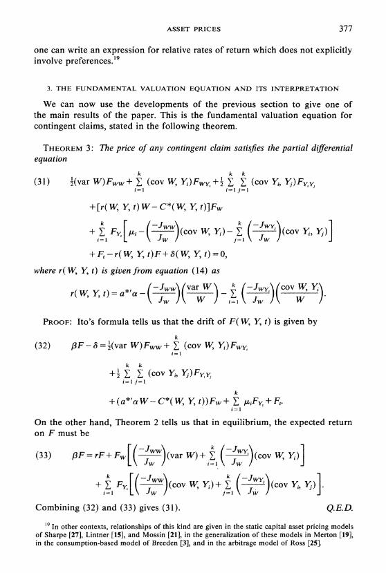
We can now use the developments of the previous section to give one of the main results of the paper. This is the fundamental valuation equation for contingent claims, stated in the following theorem.

THEOREM 3: The price of any contingent claim satisfies the partial differential equation

(31) (var W)Fww+ Z (cov W, Y,)Fw+, E Z (cov Yi, Yj)FY, Y i-1 i-1 j=l

+[r( W, Y, t)W- C*(W, Y, t)]Fw

k k - JWY.

+ E Fy, i - (cov W, Y i) ( (cov Yi, Yj) 1=1 xi- Jw j= Jw

+Ft-r(W, Y, t)F+8(W, Y, t)=0,

where r( W, Y, t) is given from equation (14) as

r(W, Y, t) = a*'o-( Jww) (varW) - -J )(co Y) iw w i=1 iw w

PROOF: Ito's formula tells us that the drift of F( W, Y, t) is given by k

(32) /3F- = (var W)Fww + (cov W, Y,)FwY, i=l

k k

+½ c (COVYi, Y)Fy,y, i=lj=l

k

+(a*'aW-C*(W, Y, t))Fw+ tLiFy + Ft. i=1

On the other hand, Theorem 2 tells us that in equilibrium, the expected return on F must be

(33) pF= rF+Fw (-Jw (var W)+E ( ')(cov W, Y) J w i=i w w

k k

+ E Fy ( )(cov W, Yi)+ ( ( Yi, Y) i=l \w jW=l W _

Combining (32) and (33) gives (31). Q.E.D.

19 In other contexts, relationships of this kind are given in the static capital asset pricing models of Sharpe [27], Lintner [15], and Mossin [21], in the generalization of these models in Merton [19], in the consumption-based model of Breeden [3], and in the arbitrage model of Ross [25].

377

378 J. C. COX, J. E. INGERSOLL, JR., AND S. A. ROSS

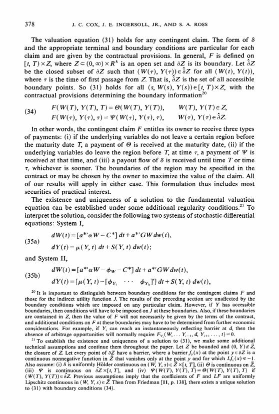
The valuation equation (31) holds for any contingent claim. The form of 8 and the appropriate terminal and boundary conditions are particular for each claim and are given by the contractual provisions. In general, F is defined on [t, T) x Z, where Z c (0, oo) x R is an open set and AZ is its boundary. Let AZ be the closed subset of AZ such that (W(r), Y(r))EiJZ for all (W(t), Y(t)), where r is the time of first passage from Z. That is, AZ is the set of all accessible boundary points. So (31) holds for all (s, W(s), Y(s))E[t, T)xZ, with the contractual provisions determining the boundary information20

F( W( T), Y( T), T) =(W( T), Y( T)), W( T), Y( T) E Z,

F( W(r), Y(,r), r) = I'( W(r), Y(r), r), W(r), Y(r) E aZ.

In other words, the contingent claim F entitles its owner to receive three types of payments: (i) if the underlying variables do not leave a certain region before the maturity date T, a payment of & is received at the maturity date, (ii) if the underlying variables do leave the region before T, at time r, a payment of IF is received at that time, and (iii) a payout flow of 5 is received until time T or time , whichever is sooner. The boundaries of the region may be specified in the contract or may be chosen by the owner to maximize the value of the claim. All of our results will apply in either case. This formulation thus includes most securities of practical interest.

The existence and uniqueness of a solution to the fundamental valuation equation can be established under some additional regularity conditions.21 To interpret the solution, consider the following two systems of stochastic differential equations: System I,

dW(t) = [a*'oaW- C*] dt+ a*'GWdw(t), 35)

dY(t) = ,u( Y, t) dt + S( Y, t) dw(t);

and System II,

(35b) dW(t) = [a*'aW- kw - C*] dt + a*'GWdw(t),

dY(t) = [,u( Y, t) - [0y . * * * OYk]'] dt + S( Y, t) dw(t), 20 It is important to distinguish between boundary conditions for the contingent claims F and

those for the indirect utility function J. The results of the preceding section are unaffected by the boundary conditions which are imposed on any particular claim. However, if Y has accessible boundaries, then conditions will have to be imposed on J at these boundaries. Also, if these boundaries are contained in Z, then the value of F will not necessarily be given by the terms of the contract, and additional conditions on F at these boundaries may have to be determined from further economic considerations. For example, if Yi can reach an instantaneously reflecting barrier at d, then the absence of arbitrage opportunities will normally require Fy(.W,... Y> , d, Yi+j ..., t) =O.

2 To establish the existence and uniqueness of a solution to (31), we make some additional technical assumptions and continue them throughout the paper. Let Z be bounded and (0, Y) Z, the closure of Z. Let every point of aZ have a barrier, where a barrier fy(x) at the point y E dZ is a continuous nonnegative function in Z that vanishes only at the point y and for which Lf8.(x)< -1. Also assume: (i) 5 is uniformly Holder continuous on ( W, Y, s) E Z x[ t, T], (ii) 9 is continuous on Z, (iii) I is continuous on dZ x [t, T], and (iv) F( W( T), Y( T), T) = &( W( T), Y( T), T) if (W(T), Y(T)) c aZ. Previous assumptions imply that the coefficients of F and LF are uniformly Lipschitz continuous in ( W, Y, s) c Z. Then from Friedman [11, p. 138], there exists a unique solution to (31) with boundary conditions (34).

ASSET PRICES 379

where the processes solving (I) and (II) are defined on the same probability space and start from the same initial position. System (I) describes the actual movement of W(t), Y(t) until the first passage to W=0, while System (II) describes the movement of a similar process when the drifts are altered by the factor risk premiums. Assume that the coefficients are extended from (0, oo) x Rk into Rk+1 in any arbitrary way such that the regularity conditions of footnote 4 are satisfied and positive values of W are inaccessible from a nonpositive initial position. Our interest will be limited to the behavior of I and II in Z Each of the processes j, j = 1, 2, induces a probability HA on (CkT l, QT), where CT 1 is the space of continuous functions f(s) from [t, T] into Rk+l and QT is the cr-algebra generated by the sets (f(s) E B), where B is any Borel set in Rk+l and s c[t, T].

Systems I and II can be used to give probabilistic interpretations of the solution to the valuation equation (31). These are contained in the following two lemmas.

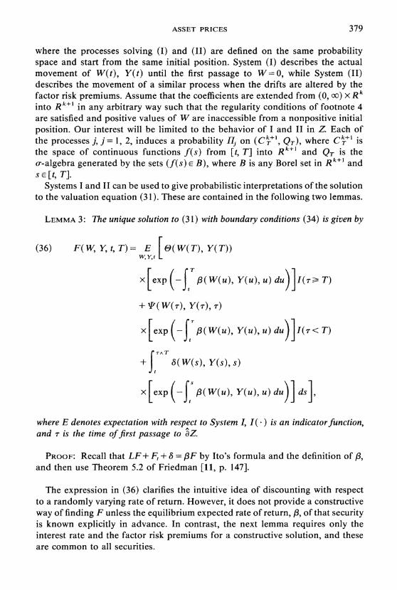
LEMMA 3: The unique solution to (31) with boundary conditions (34) is given by

(36) F(W, Y, t, T)= E [&(W(T), Y(T)) WI Y, t

+'tfr(W(r), YQr),rT)

C TA T

+ J I ( W (s), Y(s), s)

x [exp (-| J (W(u), Y(u), u) du)] ds],

where B denotes excpectation with respect to System I, I( ) is anl indicator function, and r is the time of first passage to AZ.

PROOF: Recall that LEF F, +86= f3F by Ito's formula and the definition of 3, and then use Theorem 5.2 of Friedman [11, p. 147].

The expression in (36) clarifies the intuitive idea of discounting with respect to a randomly varying rate of return. However, it does not provide a constructive way of finding F unless the equilibrium expected rate of return, /3, of that security is known explicitly in advance. In contrast, the next lemma requires only the interest rate and the factor risk premiums for a constructive solution, and these are common to all securities.

380 J. C. COX, J. E. INGERSOLL, JR., AND S. A. ROSS

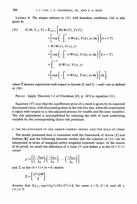
LEMMA 4: The unique solution to (31) with boundary conditions (34) is also given by

(37) F( W, Y, t, T) =E w yt [ (W( T), Y( T))

+lI'(W(r), Y(r),rT)

x [exp (-f r( W(u), Y(u), u) du) I (r < T)

r TA T

+ J 8(W(s), Y(s), S)

x [exp (-f r(W(u), Y(u), u) du)] ds],

where E denotes expectation with respect to System II, and I(*) and r are as defined in (36).

PROOF: Apply Theorem 5.2 of Friedman [11, p. 147] to equation (31).

Equation (37) says that the equilibrium price of a claim is given by its expected discounted value, with discounting done at the risk free rate, when the expectation is taken with respect to a risk-adjusted process for wealth and the state variables. The risk adjustment is accomplished by reducing the drift of each underlying variable by the corresponding factor risk premium.

4. THE RELATIONSHIP TO THE ARROW-DEBREU MODEL AND THE ROLE OF FIRMS

The model presented here is consistent with the framework of Arrow [1] and Debreu [8], and the following theorem verifies that the solution of (31) can be interpreted in terms of marginal-utility-weighted expected values. In the course of its proof, we recall the definition of L from (7) and define X as the (k+ 1) x 1 vector

and E as the (k + 1) x (n + k) matrix

[a*'GW

lS J

Assume that EwY ,exp (Adx(s).(s)I2)d, for some A >0, d >0, and all s, t ss T

ASSET PRICES 381

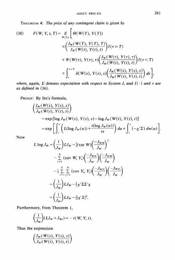
THEOREM 4: The price of any contingent claim is given by

(38) F(W, Y, t, T)= E O( W(T), Y(T)) W,Y,t _

x(Jw( W( ), Y( ), ) ))I(r > T) x Jw(W(t), Y(t), t)

) [pJw(W(t), Y(t), t))

+ T( W(r) Y( ) Jw (W(t), Y(t), t)

+ 6^Ta(W( ) y( ) ,l/w(W(s), Y(s), s) ds + ( Jw( W(s), Y(s), st)

where, again, E denotes expectation with respect to System I, and I( ) and r are as defined in (36).

PROOF: By Ito's formula,

(Jw(W(s), Y(s),s)) Jw( W(t), Y(t), t))

= exp [log Jw(W(s), Y(s),s)- log Jw( W(t), Y(t), t)]

exp ~ a(log Jw(u)) s = exp L(log Jw(u))+ (log

)))du+ (-X') dw(u)

Now

L log Jw = LJ -(var W)(

Jw )(

Furthermore, from Theorem 1,

k k Jww /

) (L Jw)=-r( W , Y,t).

Thus the expression

fJw(W(s), Y(s), s) \Jw( W(t), Y(t), t)

382 J. C. COX, J. E. INGERSOLL, JR., AND S. A.. ROSS

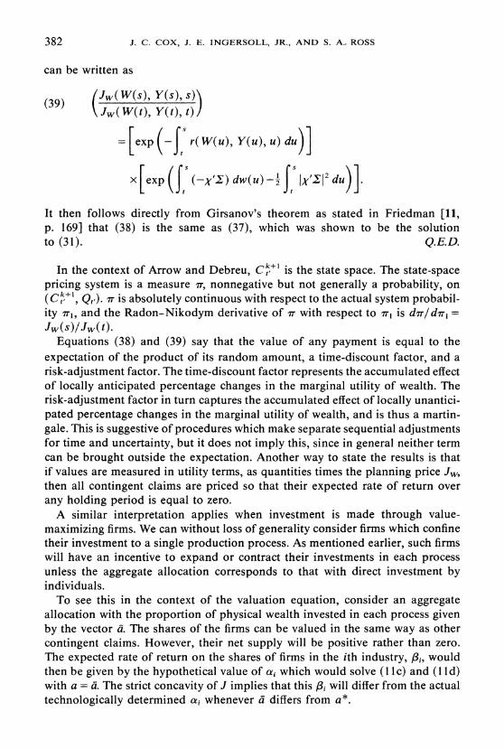
can be written as

(3) w( W(S), Y(s), S)\ _, JW(W(t), Y(t), t)

-[exp (- r(W(u), Y(u), u) du)]

x[exp ({ (-X's) dw(u) IX IX'L12 du)]

It then follows directly from Girsanov's theorem as stated in Friedman [11, p. 169] that (38) is the same as (37), which was shown to be the solution to (31). Q.E.D.

In the context of Arrow and Debreu, Ct,+ is the state space. The state-space pricing system is a measure ir, nonnegative but not generally a probability, on (Ct,', Qt). ir is absolutely continuous with respect to the actual system probabil- ity 7r1, and the Radon-Nikodym derivative of v with respect to 7rT is dir/dir1 =

JW(S)/JW(t) Equations (38) and (39) say that the value of any payment is equal to the

expectation of the product of its random amount, a time-discount factor, and a risk-adjustment factor. The time-discount factor represents the accumulated effect of locally anticipated percentage changes in the marginal utility of wealth. The risk-adjustment factor in turn captures the accumulated effect of locally unantici- pated percentage changes in the marginal utility of wealth, and is thus a martin- gale. This is suggestive of procedures which make separate sequential adjustments for time and uncertainty, but it does not imply this, since in general neither term can be brought outside the expectation. Another way to state the results is that if values are measured in utility terms, as quantities times the planning price Jw, then all contingent claims are priced so that their expected rate of return over any holding period is equal to zero.

A similar interpretation applies when investment is made through value- maximizing firms. We can without loss of generality consider firms which confine their investment to a single production process. As mentioned earlier, such firms will have an incentive to expand or contract their investments in each process unless the aggregate allocation corresponds to that with direct investment by individuals.

To see this in the context of the valuation equation, consider an aggregate allocation with the proportion of physical wealth invested in each process given by the vector a The shares of the firms can be valued in the same way as other contingent claims. However, their net supply will be positive rather than zero. The expected rate of return on the shares of firms in the ith industry, f8i, would then be given by the hypothetical value of ai which would solve (11 c) and (11 d) with a a. The strict concavity of J implies that this 8i will differ from the actual technologically determined cai whenever a differs from a*.

ASSET PRICES

The amount of the good held by a firm continually reinvesting its output in the ith process could then be taken as an additional state variable having an expected rate of return of ai. By applying the valuation equation to this firm, we find that its market value is equal to the physical amount of the good it holds plus the value of a continual payout stream of ai - ,i. The market value of a firm will thus differ from the physical amount of the good that it holds whenever ai ,3i. Consequently, all firms will be in equilibrium, with no incentive to expand or contract their investments, only when a = a*.

5. CONCLUDING COMMENTS

In this paper, we have developed a general equilibrium model of a simple but complete economy and used it to study asset prices. One of our principal results was a partial differential equation which asset prices must satisfy. The solution of this equation determines the equilibrium price of a given asset in terms of the underlying real variables in the economy. By combining this solution with prob- abilistic information about the underlying variables, one can answer a wide variety of questions about the stochastic structure of asset prices.

We have intentionally kept our model as streamlined as possible in order to concentrate on the most important issues. A number of additional features could be added in a straightforward way. For example, we could introduce multiple goods or nonlinear production technologies. As another example, we could examine how the tradeoff between labor and leisure would affect asset prices by including labor in the production function and leisure in the direct utility function.

A further generalization follows from the fact that we are free to introduce state variables which do not affect production opportunities but are nevertheless of interest to individuals. There is no reason why the movement of these additional state variables could not be influenced by individual consumption decisions. Consequently, we could define the state variables as particular functions of past consumption. For example, if we specified dYj(t)= C(t) dt, then the change in Yj over any period would be the integral of consumption over that period. Further flexibility could be obtained by including a state-dependent utility of terminal wealth function, B(W(t'), Y(t')). As a simple example, the specification U(C(s), Y(s)) = 0, B(W(t'), Y(t')) = yYj(t'), and dYj(t) = [y log C(t)]Yj(t) dt, with y a constant less than one, would correspond to the multiplicative utility functions studied in Pye [23]. In this way, we could introduce many types of intertemporal dependencies in preferences while still maintaining the tractability of our basic model.

Massachusetts Institute of Technology and

Yale University

Manuscript received September, 1978; revision received October, 1984.

383

384 J. C. COX, J. E. INGERSOLL, JR., AND S. A. ROSS

REFERENCES

[1] ARROW, K. J.: "The Role of Securities in the Optimal Allocation of Risk Bearing," Review of Economic Studies, 31(1964), 91-96.

[2] BLACK, F., AND M. SCHOLES: "The Pricing of Options and Corporate Liabilities," Journal of Political Economy, 8 1(1973), 637-654.

[3] BREEDEN, D. T.: "An Intertemporal Asset Pricing Model with Stochastic Consumption and Investment Opportunities," Journal of Financial Economics, 7(1979), 265-296.

[4] BROCK, W. A.: "An Integration of Stochastic Growth Theory and the Theory of Finance, Part 1: The Growth Model," in General Equilibrium, Growth, and Trade, ed. by J. R. Green and J. A. Scheinkman. New York: Academic Press, 1979.

[5] "Asset Prices in a Production Economy," in The Economics of Information and Uncer- tainty, ed. by J. J. McCall. Chicago: University of Chicago Press, 1982.

[6] CONSTANTINIDES, G. M.: "Admissible Uncertainty in the Intertemporal Asset Pricing Model," Journal of Financial Economics, 8(1980), 71-86.

[7] Cox, J. C., J. E. INGERSOLL, JR., AND S. A. Ross: "A Theory of the Term Structure of Interest Rates," Econometrica, 53(1985), 385-407.

[8] DEBREU, G.: The Theory of Value. New York: John Wiley, 1959. [9] DONALDSON, J. B., AND R. MEHRA: "Comparative Dynamics of an Equilibrium Intertemporal

Asset Pricing Model," Review of Economic Studies, 51(1984), 491-508. [10] FLEMING, W. H., AND R. W. RISHEL: Deterministic and Stochastic Optimal ControL New York:

Springer-Verlag, 1975. [11] FRIEDMAN, A.: Stochastic Differential Equations and Applications, Volume l. New York:

Academic Press, 1975. [12] GIHMAN, I. I., AND A. V. SKOROHOD: Stochastic Differential Equations. New York: Springer-

Verlag, 1972. [13] HARRISON, J. M., AND D. M. KREPS: "Martingales and Arbitrage in Multiperiod Securities

Markets," Journal of Economic Theory, 20(1979), 381-408. [14] HUANG, C.: "Information Structure and Equilibrium Asset Prices," Journal of Economic Theory,

forthcoming. [15] LINTNER, J.: "The Valuation of Risky Assets and the Selection of Risky Investments in Stock

Portfolios and Capital Budgets," Review of Economics and Statistics, 47(1965), 13-37. [16] LUCAS, R. E., JR.: "Asset Prices in an Exchange Economy," Econometrica, 46(1978), 1426-1446. [17] MERTON, R. C.: "Optimum Consumption and Portfolio Rules in a Continuous Time Model,"

Journal of Economic Theory, 3(1971), 373-413. [18] : "Rational Theory of Option Pricing," Bell Journal of Economics and Management Science,

4(1973), 141-183. [19] "An Intertemporal Capital Asset Pricing Model," Econometrica, 41(1973), 867-887. [20] : "On the Pricing of Contingent Claims and the Modigliani-Miller Theorem," Journal of

Financial Economics, 5(1977), 241-249. [21] MOSSIN, J.: "Equilibrium in a Capital Asset Market," Econometrica, 34(1966), 768-783. [22] PRESCOTT, E. C., AND R. MEHRA, "Recursive Competitive Equilibrium: The Case of

Homogeneous Households," Econometrica, 48(1980), 1365-1379. [23] PYE, G.: "Lifetime Portfolio Selection in Continuous Time for a Multiplicative Class of Utility

Functions," American Economic Review, 63(1973), 1013-1016. [24] RICHARD, S. F., AND M. SUNDARESAN: "A Continuous Time Equilibrium Model of Forward

Prices and Futures Prices in a Multigood Economy," Journal of Financial Economics, 9(1981), 347-371.

[25] Ross, S. A.: "The Arbitrage Theory of Capital Asset Pricing," Journal of Economic Theory, 13(1976), 341-360.

[26] RUBINSTEIN, M. E.: "The Valuation of Uncertain Income Streams and the Pricing of Options," Bell Journal of Economics, 7(1976), 407-425.

[27] SHARPE, W. F.: "Capital Asset Prices: A Theory of Market Equilibrium under Conditions of Risk," Journal of Finance, 19(1964), 425-442.

[28] STAPLETON, R. C., AND M. G. SUBRAHMANYAM: "A Multiperiod Equilibrium Asset Pricing Model," Econometrica, 46(1978), 1077-1096.