asedisas

thosee tossets ofors’d byrs’and

cingral-atstors

set-thewithen

aren are

Introduction

This paper attempts to provide a survey of asset-pricing models bon the principle of maximization of expected utility. I will begin my analysby setting out a simplified, discrete-time version of the model that wdeveloped independently by Lucas (1978) and Breeden (1979). Sincestudies appeared, intertemporal general-equilibrium models have comoccupy an increasingly important place in the economic literature on apricing. A common characteristic of those models is that prices and yieldfinancial assets are linked, in a general-equilibrium context, to investdecisions about consumption and savings. The yield structure predictethese models is therefore intimately tied to the nature of investopreferences and, in particular, to the parameters of risk aversionintertemporal substitutions. Moreover, in contrast to the capital-asset-pri(CAPM) model of Sharpe (1964) and Lintner (1965), intertemporal geneequilibrium models identify clearly the underlying economic forces thinfluence the risk-free real interest rate and the compensation that inveearn by accepting risk.1

My analysis begins in Section 1 by developing a fundamental aspricing equation derived from the Lucas model. This equation linksexcess return expected from a risky asset to the covariance of its yieldthe intertemporal marginal rate of substitution of consumption. I will th

1. The CAPM model deals with the question of how asset prices and yieldsdetermined, under the hypothesis that the risk-free interest rate and market returvariables determined outside the model.

Asset Pricing in Consumption Models: ASurvey of the Literature

Benoît Carmichael

3

4 Carmichael

ithnces

oraland

h aceseal

orspotactriskhecalmodeles failtion.

isof antyk of. Intheof

, onthe

s oftivesk of

yings byhaveichillionsee

discuss in detail the extent to which this restriction is compatible wobserved empirical phenomena. We shall see, in particular, that preferethat fail to dissociate the concepts of risk aversion and intertempsubstitution cannot explain simultaneously the level of real interest ratesthe level of the equity premium. I will conclude the second section witbrief discussion of two possible modifications to the structure of preferenthat bring the model more in line with reality, especially regarding the rinterest rate level.

Section 2 looks at the pricing of zero-coupon discount bonds“strip” bonds. I focus here on the way prices and yields are set on theand forward markets. First, I will show that the price of a forward contris, in general, a combination of the expected future spot price plus apremium. I will then examine to what extent the level and variability of trisk premiums predicted by the model are compatible with empiriobservations. Once again, there are some major tensions between theand the data. These are especially apparent when investors’ preferencto dissociate the concepts of risk aversion and intertemporal substituThe section concludes with a brief discussion of options pricing.

The impact of inflation and of monetary growth on asset pricingdiscussed in Section 3. Money is introduced into the model by meansClower cash-in-advance constraint. I will show that the uncertaisurrounding the purchasing power of money modifies the systematic risfinancial assets and, in general, gives rise to an inflation-risk premiumthe case of bonds, this premium reflects solely the covariance ofmarginal rate of intertemporal substitution of consumption with the rateappreciation of the purchasing power of money. In the case of equitiesthe other hand, it also reflects the impact of the inflation tax path onuncertainty surrounding future returns in the form of capital gains.

1 Prices and Returns in Consumption Models

1.1 The Lucas model

In this section of the literature survey I develop the basic elementthe consumption model as it relates to asset pricing. The primary objechere are: to understand the factors that determine the systematic risfinancial assets in this type of model; and to isolate the factors underlthe determination of the real interest rate. I will address these questionmeans of a discrete-time model proposed by Lucas (1978). Once Ideveloped the model’s structure, I will examine in detail the extent to whthe model’s predictions are consistent with reality. In particular, I wconclude that this type of model requires a high coefficient of risk aversin order to explain the observed level of risk premiums. We shall also

Asset Pricing in Consumption Models: A Survey of the Literature 5

ealersionven

ar an

ofuireve aerendsat

esal

stor

sfy,

tility

that the model’s predictions are compatible with a relatively low level of rinterest rates, as long as preferences dissociate the concepts of risk avand intertemporal substitution. A synthesis of the Lucas model is gibelow.

Lucas analyzes the portfolio and consumption choices ofrepresentative agent who maximizes expected intertemporal utility oveinfinite planning horizon. For each period, this agent has the choiceinvesting in two different kinds of financial assets. The agent can acqequities, which promise an uncertain return, or invest in bonds, which hafixed yield that is known in advance. In this first section, I assume that thareJ equities in circulation, and that the only bonds available are strip bowith a certain term to maturity. The portfolio choice facing the agent, whothe beginning of periodt has a portfolio containing bonds and sharof J stocks, gives rise to the following dilemma of intertempormaximization:

, (1)

under the constraint that

, (2)

where: is the investor’s momentary utility function;2 isconsumption in periodt; is the price of the equityj at periodt after thedistribution of dividends; and are the price at periodt of a bondguaranteeing return of a unit of consumption at period ; and isthe conditional expectations operator for all the information that the invepossesses at periodt.

Lucas (1978) shows that the agent’s optimum portfolio must satifor each period, the following two Euler conditions:

(3)

2. The instantaneous utility function has the usual characteristics: the marginal uof consumption is positive but decreasing, and Inada conditions are respected.

bτ zτj

MAX Et βτ−tU Cτ( )

τ t=

∞

∑zτ

jbτ Cτ, ,

0 β ∞< <

Cτ qτzj

j 1=

J

∑ • zτ+1j

qτf

• bτ+1 Dτj

qτzj+ • zτ

jbτ+

j 1=

J

∑≤++

τ t … ∞, ,=

U •( ) Cτqτ

zj

Dτj qτ

f

t 1+ Et •

U′ •t( ) • qtzj βEt U′ •t+1( ) • Dt+1

jqt+1

zt+ = j 1 … J, ,=

6 Carmichael

In

h

entthis

izesnefitfis

nt at

entess)rginal

andndthe

. (4)

Conditions (3) and (4) have the following intuitive interpretations.the first of these two conditions, an investor who acquires at periodt anadditional share of equityj must sacrifice units of consumption, whicat the margin generates a utility loss equal to

units. This investment, however, will bring, in period , capital andinterest equal to

units, the consumption of which will enhance the investor’s welfare by

units. Given the uncertainty of this return, and the fact that the agdiscounts future utility by a factor , the marginal benefit expected frominvestment is equal to

.

Condition (3) therefore simply expresses the fact that the agent optimportfolio management by equalizing the marginal cost and marginal beof investment in equityj. Similarly, an agent who buys an additional unit othe safe asset in periodt must reduce current consumption by units. Thproduces an immediate utility loss of

units. That loss, however, is offset by the gain realized on this investmeperiod . This gain is equal to

units of expected utility. Once again, condition (4) shows that efficiportfolio management requires the agent to invest in safe (i.e., risklassets up to the break-even point between the marginal benefit and macost of the investment.

The consumption model’s predictions about the pricing of bondsequities flow from a general-equilibrium estimation of conditions (3) a(4). To this point, we have discussed conditions (3) and (4) solely from

U′ •t( ) • qtf βEt U′ •t+1( )=

qtzj

U′ •t( ) • qtzj

t 1+

Dt+1j qt+1

zj+( )

U′ •t+1( ) • Dt+1j qt+1

zj+( )

β

βEt U′ •t+1( ) • Dt+1j qt+1

zj+( )

qtf

U′ •t( ) • qtf

t 1+

βEt U′ •t+1( )

Asset Pricing in Consumption Models: A Survey of the Literature 7

rentust

on allodel,

illing

ive

rveits aretedf thetilityrentingetriclityisk-

l.e.,tyrigidncesptionoralof

only

perspective of individual choices, where the market values (i.e., the curprices) of assets are given. Under general equilibrium, prices mconstantly adjust to maintain the balance between supply and demandmarkets simultaneously. In the specific case of a representative-agent mmarket equilibrium is reached when:

(5)

(6)

; (7)

that is to say, when the agent: consumes all economic endowment; is wto hold all equities in circulation; and carries no debt.

In this literature, the momentary utility function for a representatagent often takes the following isoelastic form:

, (8)

where the parameter is the Arrow–Pratt risk-aversion coefficient.

The utility function (8) has several interesting properties that deseexamination. First, (8) is compatible with risk neutrality (i.e., ), andalso includes, when tends towards unity, the case where preferencelogarithmic. Second, with this functional form, the risk premiums predicby the model are resistant to changes in wealth levels and in the size oeconomy. Third, to the extent that economic agents share the same ufunction, we can aggregate individual choices, even if agents have diffelevels of wealth. This property offers some theoretical support for usaggregate consumption, rather than individual consumption, in economstudies on the determination of returns. Finally, with the isoelastic utifunction, the parameter determines simultaneously the relative raversion coefficient and the elasticity of intertemporal substitution, .

In fact, with this functional form, the elasticity of intertemporasubstitution is the reciprocal of the relative risk-aversion coefficient (i

). Hall (1988) points out that this property of the isoelastic utilifunction is not necessarily desirable. In theory, there should be no suchlink between these two distinct preference aspects. Risk aversion influethe rate at which the agent is prepared to exchange units of consumbetween different states of nature, whereas the elasticity of intertempsubstitution reflects the agent’s willingness to exchange unitsconsumption between periods. Risk aversion is a notion that can exist

Ct Dtj

j 1=

J

∑=

ztj 1= j 1 … J, ,=

bt 0=

U C( ) C1−γ

1 γ–------------=

γ

γ 0=γ

γρ

γ 1 ρ⁄=

8 Carmichael

sion.n aoralre-raneus

s ofonsky

heof

thes are

ofted

tion

sed

in the presence of uncertainty, and it need not have a temporal dimenOn the other hand, the notion of intertemporal substitution arises isituation of full certainty, even if it makes no real sense in an atempsetting. At the end of this section we shall look at two alternative and mogeneral formulations of preferences, attributable to Campbell and Coch(1995), Epstein and Zin (1989 and 1991), and Weil (1989), which allowto dissociate these two important aspects of preferences.

The consumption model’s predictions about the prices and returnbonds and equities flow from a general-equilibrium estimation of conditi(3) and (4). Ignoring speculative bubbles, the equilibrium prices for risand safe assets are given by the following two equations:

(9)

. (10)

Equation (10), which follows directly from condition (4), suggests that tequilibrium price of bonds reflects the expected marginal rateintertemporal substitution of consumption. Note that this equation linksprice of bonds to the predicted growth of consumption when preferenceisoelastic, i.e.:

.

The equilibrium value of is obtained by recursive substitutionsequation (3). In this model, is equal to the present value of expecfuture dividend flows, where the discount factor for dividends in periodis the expected marginal rate of intertemporal substitution of consumpbetween periodst and .

Alternatively, the first-order conditions (3) and (4) may be expresin terms of asset yields. Let us define

as the gross return on equityj between the periodst and , and

qtzj Et

βiU′ Ct+i( )U′ Ct( )

---------------------- • Dt+ij

i 1=

∞

∑=

qtf Et βiU′Ct+1

U′Ct------------------=

βU′ Ct+1( )U′ Ct( )

----------------------- β •Ct+1

Ct-----------

−γ

=

qtzj

qtzj

t i+

t i+

1 rt+1zj+ Dt+1

jqt+1

zj+ qt

zj⁄=

t 1+

1 rt+1f

+ 1 qtzj⁄=

Asset Pricing in Consumption Models: A Survey of the Literature 9

tion,

e of

n;”). Inuntacttion.sidethe

iourturn

t areerestte of

weption,

as the gross return on bonds over the same time span. After manipulaconditions (3) and (4) become:

(11)

, (12)

where the variable represents, for brevity’s sake, the marginal ratintertemporal substitution of consumption

.

Equation (11) is often identified as the “canonical asset-pricing equatiosee for example Ferson (1995) and Campbell, Lo, and MacKinlay (1997this equation, the variable plays the role of a stochastic discofactor.3 In a consumption model, the stochastic discount factor is in fassimilated into the consumer’s marginal rate of intertemporal substituNote as well that the riskless return, , appears in equation (12) outthe mathematical expectations operator, because it is known frombeginning of periodt.

Conditions (11) and (12) impose several restrictions on the behavof expected real returns on bonds and equities. We shall now discuss inthe role played by each of these restrictions, beginning with those thaimposed on the real interest rate. Equation (12) shows that the real intrate—the return on riskless assets—is determined by the marginal raintertemporal substitution of consumption.

. (13)

We can delve further into the restrictions imposed by this equation ifassume that preferences are of the isoelastic kind, and that consumfollows a conditional lognormal distribution. Under these two assumptionsequation (13) becomes4

3. This variable is also sometimes known as the “asset-pricing kernel.”

4. A variable that follows a conditional lognormal law has the property that

.

1 Et St t+1, • 1 rt+1zj+

= j 1 … J, ,=

1 Et St t+1, • 1 rt+1f

+ =

St t+1,

βU′ Ct+1( )U′ Ct( )

-----------------------

St t+1,

rt+1f

rt+1f

Et St t+1, 1–

1–=

χ

lnEtχ Et lnχ 1

2--- • Vart lnχ( )+=

10 Carmichael

hreeent’scastentheely

forwhenis

risk-

bywillferscanplus

the

ingf aits

ofanscted

an. Thethethe

. (14)

From (14) it can be seen that the real interest rate is determined by tseparate factors. First, the real interest rate tends to be high if , the agtime preference, is great. Second, the real interest rate is high if the foregrowth rate of consumption is high, since in this case the agwill be inclined to borrow on the credit market in order to smooth out tconsumption profile. The importance of this second effect is inversproportionate to the elasticity of intertemporal substitution. Finally,reasons of precautionary savings, the real interest rate tends to be low

, the conditional variance of the consumption growth rate,high. The strength of this effect depends on the square of the relativeaversion coefficient.

We shall now turn our attention to the restrictions imposedequation (11) on the expected return on equities. In particular, weisolate the condition under which the expected return on equities diffrom the real interest rate. Using the definition of a covariance, weexpress the right-hand side of equation (11) as a product of expectationsa covariance term. Thus:

. (15)

Next, equations (13) and (15) let us isolate predictions concerningspread between risky and riskless returns:

. (16)

Equation (16) is an alternative form of the canonical asset-pricequation. This highlights the general measure of the systematic risk orisky assetj in a consumption model. An asset is considered to be risky ifexcess return has a negative covariance with the marginal rateintertemporal substitution of consumption. A negative covariance methat the asset tends to offer a higher (lower) excess return than expewhen the marginal utility of consumption is weaker (stronger) thexpected, i.e., when consumption is stronger (weaker) than expectedrisk is systematic in the sense that it is linked to the rate of growth ofmarginal utility of aggregate consumption. In the specific case where

rt+1f δ γ • Et ∆ct+1

γ2

2----- • vart ∆ct+1( )–+=

δ

Et ∆ct+1

Vart ∆ct+1( )

1 Et St t+1, • Et 1 rt+1zj+ covt St t+1, 1 rt+1

zj+, +=

Et rt+1zj rt+1

f– 1 rt+1

f+

• covt St t+1, rt+1zj rt+1

f–,

–=

Asset Pricing in Consumption Models: A Survey of the Literature 11

er to

ionont

eturnskowsiskonnotone.st beetif its

ely,m by

turns, orateover

ed byte ahenoint889–dardardium

r this

ust

agent’s preferences are isoelastic, we can take this relationship furthshow that

. (17)

Here, is the conditional standard deviation of the consumptgrowth rate, is the conditional standard deviation of the returnrisky assetj, and is the conditional correlation coefficienbetween and . Equation (17) shows that the expected excess roffered by the risky assetj depends on three different elements. Ripremiums depend first on the quantity of risk being assumed. This flfrom and . Risk premiums depend secondly on agents’ rsensitivity which, in turn, is determined by the relative risk-aversicoefficient . Finally, the presence of risk, and sensitivity to it, doesnecessarily mean that a risky asset will yield a higher return than a safeIn order for that to be the case, the return on the asset in question mupositively correlated with the non-diversifiable risk factor . A risky assmay even offer a negative premium and yield less than a safe asset,return is negatively correlated with the consumption growth rate. Intuitivit is advantageous for agents to hold such an asset, since it protects theoffering a relatively higher return during periods of falling consumption.

1.2 Extensions of the Lucas model

The restrictions imposed by equation (16) on expected excess reconflict with several empirical observations. The best known of thesecourse, is the “equity-premium puzzle.” Mehra and Prescott (1985) estimthat the average annual excess return on all equities in the United Statesthe 1889–1978 period was 6.18 per cent. Calibration exercises conductMehra and Prescott, and by others, show that it is very difficult to generasignificant premium (more than 2 per cent) with isoelastic preferences wthe risk-aversion coefficient is kept below 10. Mehra and Prescott’s pcan be readily demonstrated using equation (17). Given that, over the 11978 period, the correlation between and is about 0.4, the standeviation of the consumption growth rate is 0.036, and the standdeviation of excess market returns is 0.167, an average overall risk premof 6.18 per cent is only possible, according to (17), if .5 Mehra andPrescott consider such a value to be beyond “reasonable” bounds fo

5. Mankiw and Zeldes (1991) show that the required aversion coefficient mapproach 100 when the sample is limited to the post-war period.

Et rt+1zj rt+1

f– γ • corrt ∆c r

zj, • σt ∆c

• σt rzj

=

σt ∆c( )σt r

zj( )corrt ∆c r

zj,( )∆c r

zj

σt ∆c( ) σt rzj( )

γ

∆c

∆c rm

γ 25=

12 Carmichael

umstedion

rns,andith aeryery4) isand

is asthe

tive,

ll butd onhemaerm

andU.S.s truen allthatwith

nt,twoted

stedIn

ultsing

lems.lainheir

ity-

parameter, in light of the microeconomic literature on the subject.6 The factthat excess returns are positive is not in itself a problem. Positive premiflow naturally enough from equation (15). The puzzle is that the predicpremiums are too small for “reasonable” values of the relative risk-averscoefficient.7

Weil (1989) points to another puzzle, associated with riskless retuthat is illustrated by equation (14). Over the period studied by MehraPrescott, the average annual growth rate of consumption was 0.018, wvariance of 0.0013. Yet, unless the relative risk-aversion coefficient is vweak and the elasticity of intertemporal substitution is consequently vhigh, the annual average real interest rate predicted by equation (1several times higher than 0.80 per cent, the level observed by MehraPrescott between 1889 and 1978. For example, even if the value oflow as 2, equation (14) predicts a real interest rate that is higher thantime preference rate of 3.34 per cent. Hence, unless is negaequation (14) is incapable of predicting the observed real interest rate.

Several recent studies using U.S. data have shown that a smasignificant portion of the fluctuations in excess returns can be predictethe basis of information at hand at the beginning of the period. Tempirical work of Campbell (1987), Campbell and Shiller (1988), and Faand French (1988) concluded that a change in short-term or long-tinterest rates, the dividend/price ratio, and the spread between long-termshort-term interest rates can all be used to predict future movements inexcess returns. Carmichael and Samson (1996) found that the same ifor Canadian excess returns over the 1969:M1–1992:M12 period. Cathis be explained by the consumption model? Equation (17) suggestspredictable movements in excess returns should be associatedpredictable movements in and/or in . For the momehowever, empirical evidence does not support either of thesepossibilities. Moreover, calibration exercises generally produce simulapremiums that vary little compared with those observed.

In the face of these empirical problems, some authors have suggemodifications to the consumption model to make it more general.particular, they have tried to determine whether the mixed empirical resmight be attributable to the auxiliary assumptions used for deduc

6. Accepting a value of 26 as reasonable does not, however, solve all the probIn fact, Obstfeld and Rogoff (1996) show that it is especially difficult in this case to expwhy investors who are so risk-sensitive seek so little international diversification in tportfolios.

7. Kocherlakota (1996) offers an excellent survey of the literature on the equpremium puzzle.

γ

γ

γ

σt ∆c( ) corrt ∆c r j,( )

Asset Pricing in Consumption Models: A Survey of the Literature 13

asedas aIn

he

s theent

iablesthetwo

thechaboutithnot

tantthentersen

Zinandthatn inare

te istheiumfer aucerate,ionthisporaln,

eturnnd

0),, whoty of

equations (14) and (17). Essentially, consumers in the consumption-bcapital-asset-pricing model (C-CAPM) use financial assets above allmeans of smoothing out the marginal utility of consumption over time.principle, there is no constraint that would require marginal utility for tperiodt to be dependent solely on consumption for periodt. It is reasonableto assume that may also be influenced by other variables, such aconsumption of leisure or the level of consumption attained in the recpast. In this case, the covariance of excess returns with these other varwill also influence risk premiums, and may even help alleviate some ofempirical difficulties noted earlier. Research in this area has takendifferent directions.

Epstein and Zin (1989 and 1991) and Weil (1989) introducednotion of “ non-expected utility” preferences into the model. Adopting supreferences allows some loosening of the independence hypothesisthe marginal utility of consumption between different states of nature. Wsuch preferences, the marginal utility of consumption in good times isindependent of the level of consumption in bad times. Another imporproperty of Epstein and Zin’s preferences is that risk aversion andelasticity of intertemporal substitution are determined by differeparameters. Thus, in contrast to isoelastic preferences, a risk-avconsumer may still be highly willing to substitute consumptiointertemporally with non-expected utility preferences. Epstein and(1991) maintain that separating the concepts of risk aversionintertemporal substitution can help to resolve some of the anomaliesarise when preferences are isoelastic. Weil (1989) studied this questiodetail, and concludes that, with such preferences, risk premiumsdetermined by the risk-aversion coefficient, and that the real interest rainfluenced by the elasticity of intertemporal substitution. Consequently,non-expected utility hypothesis does nothing to solve the equity-prempuzzle posed by Mehra and Prescott. Yet these preferences do ofsolution to the riskless-returns puzzle. In fact, Weil manages to reprodexactly the observed levels of the equity premium and the real interestby setting the risk-aversion and elasticity of intertemporal substitutcoefficients at 45 and 0.10, respectively. A risk-aversion coefficient atvalue should produce, in the case of isoelastic preferences, an intertemsubstitution elasticity parameter of . From this observatiowe may conclude that Epstein and Zin’s preferences solve the riskless-rpuzzle by allowing for, simultaneously, high levels of risk aversion aintertemporal substitution.

In the other direction are found the works of Constantinides (199Ferson and Constantinides (1991), and Campbell and Cochrane (1995)have tried to resolve the above anomalies by introducing non-separabili

Uc •t( )

0.022 1 45⁄=

14 Carmichael

nismbutofbell

ncesed asesetionrsion

el ofthe

risks aand. Ine ofofbitsthever,hern is

ss-rsiono anith

ry orthetiontionore,thisr the

preferences over time into the model. This is done by means of a mechafor consumption habit-forming. These authors make use of the simpleintuitive idea that the utility of current consumption is not independentconsumption levels attained in past periods. In technical terms, Campand Cochrane replace the utility function (8) with the following function:

, (18)

where represents the accustomed level of consumption and influethe preferences curve. The accustomed level of consumption is modella variable that adjusts gradually to variations in consumption. With thpreferences, the marginal utility of consumption rises as consumpapproaches its accustomed level. For this reason, the risk-avecoefficient varies with the business cycle, according to this relationship:

. (19)

Equation (19) shows that a consumer’s risk aversion rises as his levconsumption approaches the accustomed level. Consequently,preferences curve parameter is no longer the only determinant ofaversion. Introducing this consumption habits mechanism also allowloosening of the close link between the concepts of risk aversionintertemporal substitution that is imposed by isoelastic preferencesparticular, the risk-aversion coefficient can be very high, even if the valu

is low, since it is the parameter that governs the elasticityintertemporal substitution. For this reason, a model with consumer hacan reproduce the observed level of the equity premium by allowingrisk-aversion premium to be high even if the parameter is weak. Howethis is not really a new solution to the equity premium puzzle, since otmodels also reproduce the level of the premium when risk aversiosignificant.

This model does, however, offer a new explanation of the risklereturns puzzle. With isoelastic preferences, an increase in the risk-avecoefficient, which is needed to reproduce the equity premium, leads tincrease in the level and the variability of the real interest rate. A model wconsumption habits gets around this problem by adding a precautiona“rainy day” savings component that will counter the upward pressure onreal interest rate. Intuitively, consumers who are aware of their consumphabits will become more averse to risk when their current consumpdrops relative to the accustomed level. This will induce them to save min order to protect themselves against any further drop. Thanks toprecautionary savings mechanism, the model can reproduce a level fo

U C X–( ) C X–( )1−η=

X η

γ t ηCt

Ct Xt–-----------------=

η η

η

Asset Pricing in Consumption Models: A Survey of the Literature 15

o the

theheionoreem

asporalteofmessticof

e thefteruzzlerisk

etterrate.wascesnd

thendrmof

gns

d instrip

ofan

ds,

real interest rate that is stable and low, and can thereby offer a solution triskless-returns puzzle.

Consumption habit-forming models also offer an explanation forvariability of estimated risk premiums. This explanation lies in tcountercyclical behaviour predicted by equation (19) for the risk-averscoefficient. At a time of recession, falling consumption makes agents msensitive to risk and thus induces higher risk premiums; this would seconsistent with observed behaviour.

To sum up, consumption models define the systematic asset riskthe covariance between asset returns and the marginal rate of intertemsubstitution of consumption. Given the low variability of aggregaconsumption, the model has difficulty explaining the relatively high levelsrisk premiums, unless very high risk aversion is assumed. This becoespecially clear when consumer–investor preferences are isoela.Modifying preferences by incorporating consumption habits or the notionnon-expected utility does not change this result. Both models reproducobserved level of the equity premium only when risk aversion is high. Amore than a dozen years of intensive research, Mehra and Prescott’s phas still not been solved, at least not within reasonable levels ofaversion.

The development of consumption models has also helped us bunderstand the factors underlying the determination of the real interestToday we can conclude that the enigma of the risk-free rate, whichidentified initially by Weil (1989), disappears when we assume preferenthat allow for the separation of the concepts of risk aversion aintertemporal substitution.

2 Prices of Other Kinds of Financial Assets

The principles developed in Section 1 are equally applicable topricing of other kinds of market-traded assets. In this section, I will expathe discussion to predictions of the model for pricing securities with a teto maturity of more than one period. I will also address the questionoptions pricing.

Looking first at bonds, I will pay particular attention to price-settinon the spot and forward markets. I will also examine the restrictioimposed on rates of return according to maturity.

Let us imagine that, in addition to the kinds of securities discussethe previous section, financial markets also offer a series of risk-freebonds with different maturities. Each bond gives the right to one unitconsumption on maturity. The existence of such securities modifiesagent’s budget constraint. Let us define as the quantity of bonbj t,

16 Carmichael

ty’stock

hers,:

ious

ntis

ndare

uality

ion

ion.

ateiveure.s ofd as

maturing inj periods, held by an agent at the beginning of periodt andas the spot price of those bonds. The budget constraint in periodt becomes

, (20)

where is the longest maturity offered on the bond market. For simplicisake, budget constraint (20) ignores the elements attributed to the smarket in our earlier analysis. Variable includes all of the agent’s otincome. Also, by definition, . For each of the available maturitieefficient portfolio management must satisfy the following Euler condition

. (21)

This condition has an interpretation similar to that developed in the prevsection. The purchase in periodt of a bond with maturityj entails at themargin a utility loss equal to units. However, this investmeallows consumption in period to rise by since in thbond can be sold at the price of those with maturity . Looked at fromperiodt, this future benefit has an expected value of

units of utility. Once again, condition (21) shows that our agent’s boportfolio is optimized when the marginal cost and benefit of investmentequal for every available maturity.

Under general equilibrium, the net offer of bonds by maturity is eqto 0, . Hence, the equilibrium spot price of a bond with maturj is obtained by recursive substitutions of equation (21):

. (22)

The equilibrium price at the end of periodt for a bond with maturityjreflects fully the marginal rate of intertemporal substitution of consumptbetween periodst and . When preferences are isoelastic, equation (22)links the price of the bonds to the expected growth rate of consumptCeteris paribus, moreover, the price of a bond with maturityj is relativelyhigh (low) when the market expects a low (high) consumption growth rbetween periodst and , because investors will seek to make massbond purchases in order to reorient their consumption profile to the futThe analytical emphasis here is on prices. I will also develop predictionthe yield to term on bonds. The yield to term of a bond, which is denote

, is entirely determined by its purchase price. Thus:

qj t,

Ct bj t+1, • qj t, yt bj t, • qj t,j 0=

N

∑+≤j 1=

N

∑+

N

ytq0 t, 1≡

U′ •t( ) • qj t, βEt U′ •t+1( ) • qj−1 t+1,= j 1 … N, ,=

U′ •t( ) • qj t,t 1+ qj−1 t+1, t 1+

j 1–

βEt U′ •t+1( ) • qj−1 t+1,

bj t+1, 0=

qj t, β jEt St t+ j,=

t j+

t j+

r j t,

Asset Pricing in Consumption Models: A Survey of the Literature 17

icht off

tsa

ture,et atne

ly

allhed

a

ationthe

ureis

ve,a

ll) a

. (23)

In effect, the yield of a strip bond is simply the constant rate at whthe bond’s price must rise in order for its value to be equal to one uniconsumption at maturity . Predictions about the term structure ointerest rates flow directly from equations (22) and (23).

I will now focus on predictions about the prices of forward contracfor bonds of varying maturities. A forward contract constitutescommitment to consummate a transaction at a specified date in the fuunder pre-established conditions. We shall define as the price speriod t for a contract for delivery in period of a bond maturing iperiod , where . The benefit realized on this contract at the timof delivery by an investor taking a long position is entiredetermined by the spread between , the spot price at periodof a bond maturing at period , and the delivery price . Portfoliomanagers have an interest in trading on the forward market untilopportunities for profit have been exhausted. This situation is reacwhen:

, (24)

the present value of the benefit expected from a long position, is nil.8 Sinceis known as of periodt, equation (24) constrains the delivery price of

forward contract to respect the following condition:

. (25)

Developing the covariance term appearing on the right-hand side of equ(25), we can show that the forward contract price is a combination ofexpected future spot price plus a risk premium:

. (26)

The forward contract price is higher (lower) than the expected futspot price when the conditional covariance between andpositive (negative). Intuitively, when the conditional covariance is positian investor taking a long position on the forward market will enter into

8. Investors are in a long (short) position if they are committed to purchase (sebond at a delivery price of .

qj t,1

1 r j t,+------------------

j=

r j t,

t j+

f n t,k

t n+t k+ n k<

t n+qk−n t+1, t n+

t k+ f n t,k

0 Et St t+n, • qk−n t+1, f n t,k–( )=

f n t,k

f n t,k

f n t,k Et St t+1,

−1

• Et St t+1, • qk−n t+n,=

f n t,k Et qk−n t+n,

1qn t,--------- • covt St t+n, qk−n t+n,,

+=

St t+1, qk−n t+n,

18 Carmichael

herhant foray aon

rice.sign

ive.nceeIntionlsof theumthe

ing

o beturn

do

nce,

contract that will deliver him an asset with a spot market value that is higthan expected when the marginal utility of consumption is also higher texpected. In this case, the forward contract is an excellent instrumensmoothing out consumption over time, and investors are prepared to ppremium for this desirable characteristic. The risk premiumforward contracts is conventionally defined as

,

the spread between the expected future spot price and the forward pEquation (26) shows that the sign of the premium is determined by theof the conditional covariance between and . In particular, apositive premium is possible only if the conditional covariance is negatBackus, Gregory, and Zin (1989) show that the sign of the covariabetween and results directly from the sign of thcovariance between and in light of equation (22).particular, a negative covariance is only possible if the autocorrelacoefficient of the marginal rate of intertemporal substitution is anegative. As we shall see below, this restriction allows some versions omodel to be rejected. Finally, it should be noted that the risk premi

is not necessarily constant, since there is nothing to preventconditional covariance that appears in equation (26) from varysystematically with the state of nature.

The factors influencing expected bond returns by maturity can alsanalyzed with the help of equation (21). We define as the actual rebetween periodst and on a bond maturing in period . In this case,

is determined entirely by the capital gain realizebetween periodst and . The first-order condition (21) constrains trespect the condition

. (27)

Because the return on a bond maturing in period is known in advai.e.,

and ,

condition (27) implies that

. (28)

fpn t,k

fpn t,k Et qk−n t+n, f n t,

k–=

qk−n t+n, f n t,k

St t+n, qk−n t+n,St t+n, St+n t+k,

fpn t,k

ht+1k

t 1+ t k+ht+1

k qk−n t+n, qk t,⁄=t 1+

1 Et St t+1, • ht+1k= 1 k N≤ ≤

t 1+

ht+11

1 q1,t⁄= q1,t E St t+1,=

Et ht+1k ht+1

1– ht+1

1• covt St t+1, ht+1

k, –=

Asset Pricing in Consumption Models: A Survey of the Literature 19

nce

rmutureall)atesctspotenil.

ncestionoralthis

ofply

dects

thends

The expected return on a bond with maturityk is different from the risklessreturn—i.e., the return on a one-period bond—if the conditional covariabetween and is other than 0.

According to the theory of expectations, the slope of the testructure of interest rates is determined by market expectations about finterest rates. The slope will be positive (negative) and rates will rise (fwith the length of maturity, when the market anticipates that interest rwill increase (decline). In this case, the delivery price of forward contrawill reflect entirely and solely the market’s expectations about future sprices. The C-CAPM model is compatible with this prediction if thconditional covariance terms appearing in equations (26) and (28) areBackus et al. (1989) studied this question, and concluded that covariaare nil when: (i) agents are risk-neutral, or (ii) marginal rates of substitu

are independent. In the first case, the marginal rate of intertempsubstitution is constant and equal to under all states of nature. Forreason, equations (22), (25), and (27) imply: (i) constant values for

, , and ,

and (ii) nil risk premiums for

, and ,

under all possible conditions. Alternatively, if marginal ratesintertemporal substitution are independent, equation (22) becomes sim

, (29)

and the price of a bond maturing inj periods is the product of expectefuture prices. Consequently, the delivery price for a forward contract reflsolely the expected future spot price of the underlying security, and sopremium is nil. For the same reason, expected returns on bobetween periodst and are independent of maturity, i.e.,

,

and maturity premiums are nil.

St t+1, ht+1k

St t+1,β

qj t, f n t,k ht+1

k

fpn t,k Et ht+1

k ht+11

–

qj t, Et St+i−1 t+i,i 1=

j

∏ Et St+i−1 t+i,i 1=

j

∏= =

Et q1 t+i−1,i 1=

j

∏=

fpn t,k

t 1+

Et ht+1k 1 Et⁄( ) St t+1,=

20 Carmichael

hlyon

ture.acts,esese

iculareralr,

icate

s inf a

andl is

iumt al.tiondel’s, then thean 7umictedonive.nt ofnce

Fortion

akly

ta touateted

Thesionlues.eory

The term structure of interest rates is one of the most thorougstudied relationships in economics and finance. The voluminous workthis question has revealed two characteristic features of the term strucOn one hand, studies show that the mean risk premium on forward contr

, is small but positive. On the other hand, evidence shows that thpremiums are highly variable and partially predictable. Both thephenomena are very robust, and do not seem to depend on any partperiod or sample. Roll (1970) and Fama (1976 and 1984) provide sevstatistics that confirm this. In their review of the literature, ShilleMcCulloch, and Huston (1987) conclude that these two phenomena indoutright rejection of the theory of expectations.

Backus et al. (1989) attempted to discover whether fluctuationbond prices and risk premiums are compatible with the predictions ogeneral-equilibrium model of the kind developed by Breeden (1979)Lucas (1978). Equations (26) and (28) show that, in principle, this modecompatible with risk premiums that are positive and variable.

The question, instead, is whether the model can explain risk-prembehaviour in quantitative terms. To examine this question, Backus ecalibrated a two-state model with isoelastic preferences. Their simulaexercises reveal two important discrepancies between the mopredictions and empirical observations. First, with isoelastic preferencesmodel appears unable to reproduce the mean risk premium observed oforward market when the risk-aversion coefficient has a value of less thor 8. This result brings to mind Mehra and Prescott’s equity-premipuzzle. Second, as noted earlier, the forward-market risk premium predby the artificial economy is positive only when the autocorrelaticoefficient of the marginal rate of intertemporal substitution is negatWith isoelastic preferences, this means that the autocorrelation coefficiethe consumption growth rate must also be negative. Yet empirical evideprovides virtually no support for a negative autocorrelation coefficient.example, during the period studied by Backus et al., the autocorrelacoefficient of the consumption growth rate in the United States was wepositive.

Backus et al. (1989) also apply econometric tests to simulated dasee whether risk premiums generated by the artificial economy fluctenough that the prediction of the theory of expectations can be rejec.Here again, the results lend little support to their version of the model.simulated data reject the theory of expectations only when the risk-averand consumption autocorrelation parameters are given extreme vaInvariably, the simulated data accept the restrictions imposed by the thof expectations when the parameters are set at reasonable levels.

fpnk

Asset Pricing in Consumption Models: A Survey of the Literature 21

turein

n iscestionthe

inedthey990),ncervedorethed Zin,isktoare

n of

int,data,eaterondl ofrest

g.s aan

re oferalso,We

athe

tssetsthercise

The results obtained by Backus et al. derive in part from the strucof preferences they used in calibrating their model. As we notedSection 1, the behaviour of the marginal rate of intertemporal substitutiointimately linked to that of the consumption growth rate when preferenare isoelastic. The smooth and unpredictable behaviour of the consumpgrowth rate is, under these circumstances, difficult to reconcile withestimated behaviour of risk premiums.

Gregory and Voss (1991) test the robustness of the results obtaby Backus et al. by adopting more general preferences. In particular,examine whether the preferences suggested by Constantinides (1incorporating consumption habits and the non-expected utility prefereproposed by Epstein and Zin (1989), allow a better match of the obsebehaviour of premiums. The simulation results show that adopting mgeneral preferences is a step in the right direction. In fact, withpreferences proposed both by Constantinides (1990) and by Epstein anwe can reproduce both the level and the variability of forward-market rpremiums. Moreover, the simulated premiums are sufficiently variableindicate rejection of the theory of expectations when the simulated datasubjected to the battery of econometric tests that led to empirical rejectiothe theory.

Yet, while these results are encouraging from a theoretical viewpothe simulations reveal significant tensions between the model and theparticularly with respect to the variability of bond prices. In fact, thstandard deviation of the simulated bond price is at best 30 times grethan that observed in the data. This simply reflects the fact that the bprice must be variable if the artificial economy is to reproduce the leveobserved risk premiums. From this viewpoint, the term structure of interates remains an enigma for general-equilibrium theory.

I will conclude this section with a brief discussion of options pricinOne of the major strengths of the consumption model is that it offerunified approach to the pricing of financial assets. More specifically,asset’s value can always be determined once we know the time structuthe payments it produces. Equation (9) is an illustration of this genprinciple. We shall now see how this principle applies to options. To dowe must first define clearly the structure of payments that options offer.shall then see how equation (9) allows us to estimate options prices.

An option gives its holder the right to buy or to sell an asset withingiven period of time, at a predetermined price. This price is known as“exercise” or “strike” price. An American-style call (put) option gives iholder the right to exercise the option and to buy (sell) the underlying asat the strike price at any time up to and including the expiry date ofoption. European-style options are more restrictive; the holder can exe

22 Carmichael

ate.s are

nntrikeathe

e.,nder

re.

tormFor

ral

reimethe

on’san

m.”

the option and acquire the underlying assets only at the option’s expiry dIn contrast to the forward contracts discussed above, then, option holdernot obligated to exercise their call or put privileges.

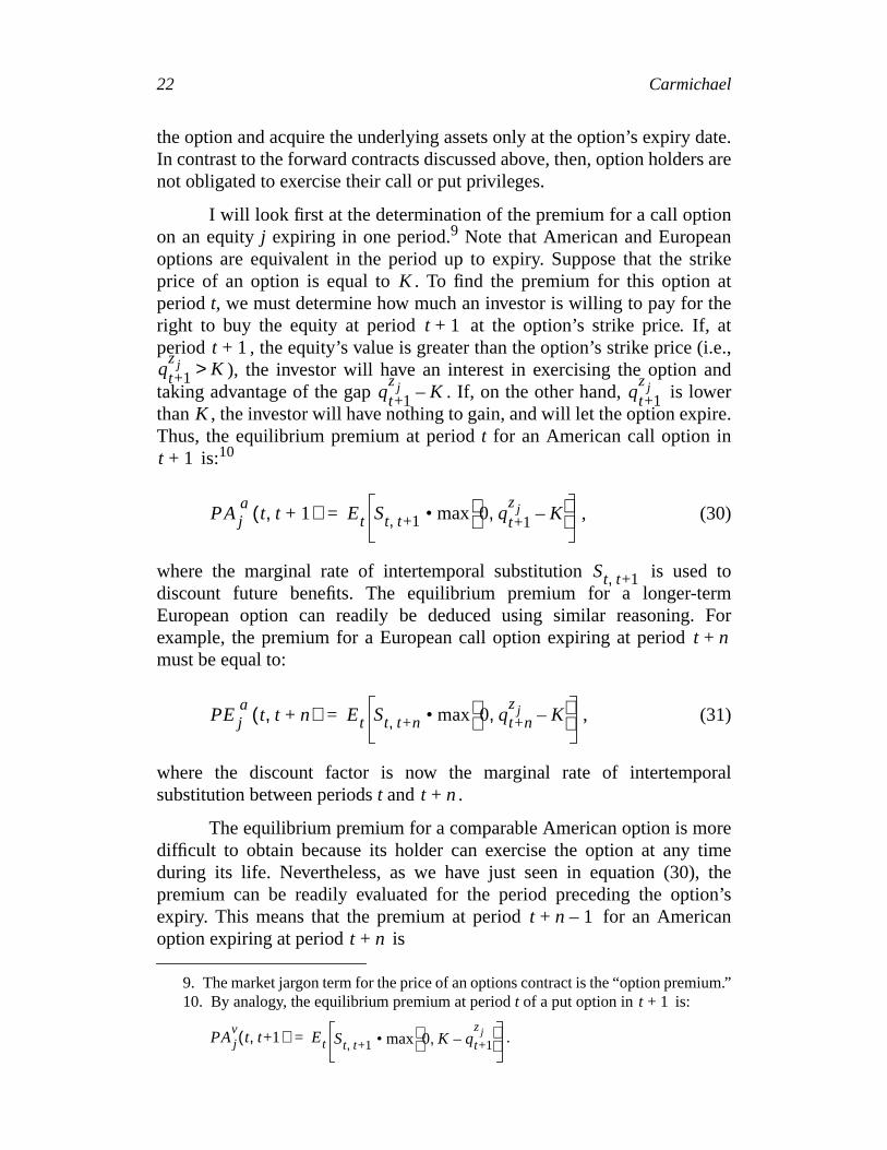
I will look first at the determination of the premium for a call optioon an equityj expiring in one period.9 Note that American and Europeaoptions are equivalent in the period up to expiry. Suppose that the sprice of an option is equal to . To find the premium for this optionperiodt, we must determine how much an investor is willing to pay for tright to buy the equity at period at the option’s strike price. If, atperiod , the equity’s value is greater than the option’s strike price (i.

), the investor will have an interest in exercising the option ataking advantage of the gap . If, on the other hand, is lowthan , the investor will have nothing to gain, and will let the option expiThus, the equilibrium premium at periodt for an American call option in

is:10

, (30)

where the marginal rate of intertemporal substitution is useddiscount future benefits. The equilibrium premium for a longer-teEuropean option can readily be deduced using similar reasoning.example, the premium for a European call option expiring at periodmust be equal to:

, (31)

where the discount factor is now the marginal rate of intertemposubstitution between periodst and .

The equilibrium premium for a comparable American option is modifficult to obtain because its holder can exercise the option at any tduring its life. Nevertheless, as we have just seen in equation (30),premium can be readily evaluated for the period preceding the optiexpiry. This means that the premium at period for an Americoption expiring at period is

9. The market jargon term for the price of an options contract is the “option premiu10. By analogy, the equilibrium premium at periodt of a put option in is:

K

t 1+t 1+

qt+1zj K>

qt+1zj K– qt+1

zj

K

t 1+

t 1+

PAjv

t t+1,( ) Et St t+1, • max 0 K qt+1

zj–, .=

PAja

t t 1+,( ) Et St t+1, • max 0 qt+1zj K–,

=

St t+1,

t n+

PEja

t t n+,( ) Et St t+n, • max 0 qt+nzj K–,

=

t n+

t n 1–+t n+

Asset Pricing in Consumption Models: A Survey of the Literature 23

illtn:

the

e ofnceThethis

ed,n is

allcetherrisktoinal

.

ofund

gap,

.

A portfolio manager who acquires this call option at period whave the choice, at period , of keeping the option, which at thatime will have a value of , or of exercising the optioand making a profit of . The equilibrium premium must then be

at period . Through a recursive process, we can deduce thatequilibrium premium for an American call option expiring in periodis:

. (32)

Generally speaking, we may conclude from equation (32) that the valuoptions in a consumption model is not independent of the prefereparameters, in particular risk aversion and intertemporal substitution.empirical results obtained by Garcia and Renault (1998) tend to confirmconclusion.

3 Inflation and Financial Markets

Up to this point, I have been examining how yields are determinwithout considering monetary factors. In many situations, this omissiojustified and unimportant. However, it cannot be ignored when analyzingthe factors underlying the yield structure. In this section, I will introdumoney into the pricing model developed earlier, in order to examine whethe risk surrounding the purchasing power of money is one of thefactors that financial markets take into account. In particular, I will trydiscover the conditions under which the real return expected from nombonds incorporates an inflation-risk premium. I will also attempt to identifythe mechanisms by which inflation affects equity prices and real returns

Discussions of monetary factors always run up against the problemscale. Macroeconomic and financial models are always short on somacroeconomic fundamentals relating to money demand. This

PAja

t n 1 t n+,–+( ) Et+n−1 St+n−1 t+n, • max 0 qt+nzj K–,

=

t n 2–+t n 1–+

PAja

t n 1 t n+,–+( )qt+n

zj K–

PAja

t n 2 t n+,–+( )

Et+n-2 St+n−2 t+n−1, • max PAja

t n 1 t n+,–+( ) qt+n

zjK–,

=

t n 2–+t n+

PAja

t t n+,( )

Et St t+1, • max PAja

t 1 t n+,+( ) qt+n

zjK–,

=

24 Carmichael

somed hocsh-

987),ings of

theoodss arethisthe

that:the

theetsicesatingthe

gentsnetaryd ofr theints,their

. Asrmtheular,ldersht to

twothethis

r thetrip

ation

however, has not prevented theoretical research from making at leastprogress on monetary questions. There are now several more or less aways of introducing money into macroeconomic models. Models with cain-advance constraints currently seem to be the most popular.11 The worksof Lucas (1982, 1984), Svensson (1985a, 1985b), Lucas and Stockey (1Labadie (1989), and Giovannini and Labadie (1991) show that introducmoney into a macroeconomic model in this way is useful as a meanisolating the financial market impact of monetary factors.

In a model with cash-in-advance constraints, transactions ongoods and services market must be paid for in money. In other words, gare exchanged for money and money is exchanged for goods, but goodnot exchanged directly for other goods. There are two major variants ofmodel that differ, depending on whether financial markets operate atbeginning or the end of the period. Lucas (1982) adopts the convention(i) agents observe existing economic conditions, as determined byavailability of goods and the rate of growth of the money supply atbeginning of the period, before taking decisions; and (ii) financial markcome into play at the beginning of the period, when the goods and servmarket is inactive. Svensson (1985b) uses the opposite scenario, activthe goods and services market at the beginning of the period andfinancial market at the end. Svensson also assumes that economic abecome aware, as soon as the goods market opens, of the value of motransfers that they will receive from the monetary authorities at the enthe period, when the financial transactions are conducted. Whatevescenario, the key factor is that, in a model with cash-in-advance constrafinancial markets are inaccessible at the time agents are makingtransactions on the goods and services market.

For purposes of analysis, I adopt the scenario proposed by Lucaswell, I will limit the discussion to the equities market and the short-tesecurities market, as I did in Section 1. However, in contrast withpreceding sections, payments are now made in money. In particrepayments of securities at maturity and dividend payments to sharehoare made in money. Financial assets are securities that give the rigmonetary payments.

Given the sequential opening of markets, agents are subject todistinct budget constraints, one for financial markets and the other forgoods and services market. Financial markets come into play first. Atpoint, agents choose their monetary transactions balances, , focurrent period, and compose their portfolios using equities and s

11. The cash-in-advance constraint first appeared in the literature with the publicof Clower (1967).

Mtd

zt

Asset Pricing in Consumption Models: A Survey of the Literature 25

get

level

t theusyeensfer

havetirelynce

eir

ust

is)ns

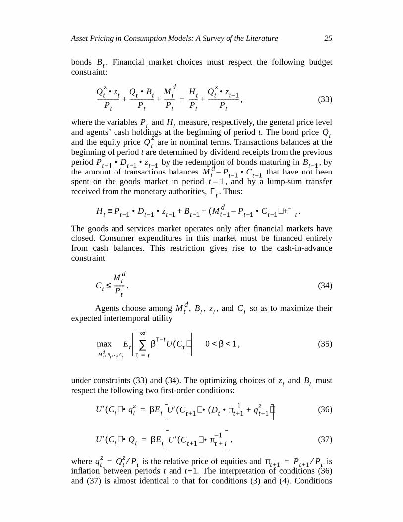
bonds . Financial market choices must respect the following budconstraint:

, (33)

where the variables and measure, respectively, the general priceand agents’ cash holdings at the beginning of periodt. The bond priceand the equity price are in nominal terms. Transactions balances abeginning of periodt are determined by dividend receipts from the previoperiod by the redemption of bonds maturing in , bthe amount of transactions balances that have not bspent on the goods market in period , and by a lump-sum tranreceived from the monetary authorities, . Thus:

.

The goods and services market operates only after financial marketsclosed. Consumer expenditures in this market must be financed enfrom cash balances. This restriction gives rise to the cash-in-advaconstraint

. (34)

Agents choose among , , , and so as to maximize thexpected intertemporal utility

, (35)

under constraints (33) and (34). The optimizing choices of and mrespect the following two first-order conditions:

(36)

, (37)

where is the relative price of equities andinflation between periodst and t+1. The interpretation of conditions (36and (37) is almost identical to that for conditions (3) and (4). Conditio

Bt

Qtz• zt

Pt----------------

Qt • Bt

Pt-----------------

Mtd

Pt--------+ +

Ht

Pt------

Qtz• zt−1

Pt----------------------+=

Pt HtQt

Qtz

Pt−1 • Dt−1 • zt−1 Bt−1Mt

d Pt−1 • Ct−1–t 1–Γt

Ht Pt−1 • Dt−1 • zt−1 Bt−1 Mt−1d Pt−1 • Ct−1–( ) Γt+ + +≡

Ct

Mtd

Pt--------≤

Mtd Bt zt Ct

max Et βτ−tU Cτ( )

τ t=

∞

∑Mt

d Bt zt Ct, , ,

0 β 1< <

zt Bt

U′ Ct( ) • qtz βEt U′ Ct+1( ) • Dt • πt+1

1–+ qt+1

z( )=

U′ Ct( ) • Qt βEt U′ Ct+1( ) • πt i+1–=

qtz Qt

z Pt⁄= πt+1 Pt+1 Pt⁄=

26 Carmichael

ingsthe

onl,’sance

evel

odsynt

cesat

theondie

the85b).nereal

ncerst-

that:

terestason,t ratelity iste issson

rtainick,ility,

t when

(36) and (37) take into account the fact that financial investment earnfluctuate with the general price level in a monetary economy—hence,presence of in these equations.

Markets are in equilibrium when: money and equities in circulatiare held willingly, and ; the net supply of bonds is ni

; and the goods market is in equilibrium, . For simplicitysake, I will restrict the discussion to the case where the cash-in-advconstraint is always binding at equilibrium.12 Under this hypothesis, thecirculation velocity of money is always constant, and the general price lobeys a strict version of the quantity theory of money:

. (38)

This hypothesis also means that inflation between perit and is equal to the quotient of the monesupply growth factor divided by the goods endowmegrowth factor .

The model’s predictions as to the effect of inflation on asset priand yields flow from the first-order conditions (36) and (37) estimatedgeneral equilibrium. Using these equations, we will explore howvariability of inflation affects the determination of prices and yieldsfinancial markets. My analysis relies in particular on the work of Laba(1989) and Giovannini and Labadie (1991), and to a lesser extent onstudies of Fama and Farber (1979), Leroy (1984), and Svensson (19I will first look at the impact on bond yields. For analysis purposes, I defithe inflation-risk premium as the spread between the expected

12. The Kuhn–Tucker multiplier associated with the cash-in-advaconstraint (34) is interpreted as the liquidity service of money. Using (37) and the fiorder condition for the choice of (an unspecified condition here) it can be shown

.

This equation demonstrates that in a cash-in-advance constraint model the nominal inrate serves to compensate investors for the liquidity shortcomings of bonds. For this rethe cash-in-advance constraint is relaxed (i.e., ) only when the nominal interesis nil. The hypothesis that the cash-in-advance constraint is always satisfied at equathus equivalent to limiting our analysis to situations where the nominal interest raalways positive. In theory, it should be possible, using the alternative scenario of Sven(1985b), to achieve an equilibrium where the liquidity constraint is relaxed under ceconditions, even if the nominal interest rate is positive. Simulation results from HodrKocherlakota, and Lucas (1991) show, however, that this is mainly a theoretical possibsince in practice the cash-in-advance constraint always seems to be binding, at leasthe parameters are set at “reasonable” values.

πt+1

Mtd Mt= zt 1=

Bt 0= Ct Dt=

µt

Mtd

µt

Pt----- βEt U′ •t+1( ) •

1Pt+1---------- • i t=

µt 0=

Pt

Mt

Pt-------=

πt+1 Pt +1 Pt⁄=t 1+ πt+1 ωt+1 λt+1⁄=( )

ωt+1 Mt+1 Mt⁄=λt+1 Ct+1 Ct⁄=

φt+1π

Asset Pricing in Consumption Models: A Survey of the Literature 27

The

exed, byof

thethes the

thehethehedelisa

oninalhan

, inporalary

return on a nominal bond and the risk-free real interest rate, .inflation-risk premium, by this definition, is equal to:

. (39)

The risk-free real interest rate corresponds to the real return on an indbond. In the Lucas (1982) model, is determined, as in equation (13)the reciprocal of the marginal rate of intertemporal substitutionconsumption.13 The expected real return of a nominal bond is equal to:

. (40)

According to Fisher’s theorem,

is equal to a risk-free real interest rate. By substituting in (40)equilibrium value of obtained from equation (37) and decomposingcovariance term that appears, an expression is derived that showcondition under which the Fisher theorem holds true:

. (41)

Equation (41) shows that the Fisher theorem’s validity, and henceexistence of an inflation-risk premium, relies on the value of tconditional covariance between the real return on money, , andmarginal rate of intertemporal substitution of consumption, . TFisher theorem is valid if covariance is nil. In all other cases, the mopredicts the existence of an inflation-risk premium, the sign of whichdetermined by the sign of the covariance, . Intuitively,positive (negative) means that the real returnmoney, , is generally greater (less) than predicted when the margrate of intertemporal substitution of consumption is greater (less) t

13. For this reason, is solely a function of real shocks. On the other handSvensson’s model, the real interest rate is determined by the marginal rate of intertemsubstitution of illiquid wealth, which is generally influenced by both real and monetshocks.

r t+1f

φt+1π

Et r t+1 r t+1f–=

r t+1f

r f

1 Et r t+1+

Et πt+11–

Qt---------------------=

Et r t+1

Qt

1 Et r t+1+ 1 r t+1f+

•

Et πt+11–

Et πt+11–

covt St t+1, πt+11–,( )

Et St t+1,

-------------------------------------------+

-----------------------------------------------------------------------=

πt+11–

St t+1,

covt St t+1, πt+11–,( )

covt St t+1, πt+11–,( )

πt+11–

28 Carmichael

entuse

this

raryis

ablest be

taxa

gofanonandtheaticrn

alue

iumof

y at

predicted. In this case, nominal bonds are a better (worse) investmthan indexed bonds for smoothing out consumption over time, becathey offer a high return when consumption is low.14 This analysis can becarried even further if one assumes that preferences are isoelastic. Incase,

, (42)

and the sign of the inflation premium depends on the contempocovariance between and . For example, if the inflation-risk premiumto be negative, the contemporary covariance between these two varimust be positive. In other words, inflation and monetary transfers musprocyclical.

Inflation also affects the stock market in the guise of an inflationthat is levied implicitly on dividend income. An equity yields its ownernominal dividend of at the end of periodt. This income can be usedto pay for consumption, at the earliest, in period , at a time when itsreal value will be . If , the change in the purchasinpower of money will represent either a tax of or a subsidy

to shareholders. Carmichael (1985) showed that, inenvironment without uncertainty, this inflation tax has a negative effectequity prices in steady state. In a broader framework, where the volumegrowth of the money supply are random, the uncertainty surroundingvalue of the inflation tax is an additional element that affects the systemrisk of equity investments in two ways. I will define as the real retuon an equity investment between periodst and . Taking the structure ofthe Lucas model, the value of is equal to

. (43)

Under conditions of general equilibrium, (36) means that the expected vof must satisfy the following condition:

. (44)

14. With the alternative scenario of Svensson (1985b), the inflation-risk premdepends instead on the conditional covariance of with the marginal rateintertemporal substitution of illiquid wealth, because financial markets come into plathe end of the period, after the goods and services market has closed.

πt+11–

covt St t+1, πt+11–,( ) β • covt λt+1

γ– λt+1 • ωt+11–,( )=

λ ω

Pt • Dtt 1+

Dt • πt+11– πt+1 1≠

πt+1 1>( )πt+1 1<( )

r t+1z

t 1+r t+1z

r t+1z Ct • πt+1

1– qt+1z

+

qtz

--------------------------------------- 1–=

r t+1z

1 Et r t+1z+

1 covt St t+1, r t+1z,( )–

Et St t+1,

----------------------------------------------------=

Asset Pricing in Consumption Models: A Survey of the Literature 29

issee3),form

at isthating

)uitynce,theby

allaticof

tion

henceoralf theus

sassetms

lationhat,the

As with equation (15), the systematic risk of equity investmentsdetermined by the conditional covariance between and . Tohow inflation affects this covariance, it is useful to reformulate it, using (4as a sum of the two elements representing the risk due to returns in theof dividends and returns in the form of capital gains:

. (45)

It is easy enough to explain the first covariance. Equities yield income thheld as money for a time before it is spent or invested. It is thus naturalthe risk surrounding the purchasing power of money during this waitperiod (which is determined by the covariance between andshould be one of the elements affecting the systematic risk of eqinvestments. To appreciate the impact of inflation on the second covariawe must explain the link between the equilibrium price of equities andfuture path of the inflation tax. The equilibrium value of is obtainedrecursive substitutions of equation (36):

. (46)

Solution (46), in contrast with that obtained in Section 1, is a function ofthe future expected values of the inflation tax. For this reason, the systemrisk of equity investments is also influenced, through returns in the formcapital gains, by the uncertainty surrounding the future path of the inflatax.

To sum up, in the Lucas model, the inflation risk affects tsystematic risk of equities in two ways. First, because the covariabetween the real return on money and the marginal rate of intertempsubstitution of consumption is not nil; second, because the future path oinflation tax influences the distribution of future capital gains and thmodifies the covariance between and .

In principle, the level and the variability of inflation premiums, adiscussed, here can significantly affect the stochastic process ofreturns. Could the inclusion of monetary factors and inflation-risk premiuhelp us to understand some of the anomalies set out in Section 1? Simuresults from Labadie (1989) and Giovannini and Labadie (1991) show tin qualitative terms, the inclusion of monetary factors generally steers

St t+1, r t+1z

covt St t+1, r t+1z,

qtz

1–=

• Ct • covt St t+1, πt+11–,

covt St t+1, qt+1z,

+

St t+1, πt+11–

qtz

qtz

EtSt t+1, • Ct+ j−1 • πt+ j

1–

j 1=

∞

∑=

St t+1, qt+1z

30 Carmichael

elys a

inalr ofthoseperverys inte of

s oflso

m to

ingtheiron.hownhenpt ofveenceporalencetheesectedlitys of

peasingthelow

model’s predictions in the right direction. Yet these effects are quantitativsmall when preferences are isoelastic. For example, Labadie findmaximum inflation premium at an absolute value of 0.3 per cent for nombonds. Giovannini and Labadie simulate market premiums of the orde0.42 per cent to 1.91 per cent. These values, while much greater thanfound by Mehra and Prescott (1985), are still far from the value of 6.18cent observed in the data. Moreover, the simulated premiums are notvariable. Giovannini and Labadie arrive at the conclusion that fluctuationexpected returns are essentially due to fluctuations in the marginal raintertemporal substitution of consumption.

Conclusions

This paper has attempted to review the asset-pricing predictionintertemporal models under conditions of general equilibrium. I have adiscussed the extent to which the predictions of these models conforreality.

My analysis has focused primarily on a fundamental asset-pricequation that links expected returns on assets to the covariance ofyields with the marginal rate of intertemporal substitution of consumptiThe intensive research conducted over the past 20 years has ssignificant discrepancies between the model and the data, particularly wpreferences take an isoelastic form that does not dissociate the concerisk aversion from that of intertemporal substitution. While it may not haresolved all the problems, the development of more generalized preferstructures that can dissociate the concepts of risk aversion and intertemsubstitution has nonetheless helped clarify how these two concepts influyields. I have shown that in these models risk aversion affects primarilyrisk premium, while the elasticity of intertemporal substitution determinthe real interest rate. I have also shown that models based on unexputility and on consumption habit formation are better able to explain reabecause, each in its own way, they allow simultaneously for high levelrisk aversion and of intertemporal substitution.

The introduction of monetary factors, by means of a Clower-tycash-in-advance constraint, shows that uncertainties as to the purchpower of money can modify the systematic risk of financial assets. Yetsimulation results obtained to date reveal inflation premiums that areand not very variable.

Asset Pricing in Consumption Models: A Survey of the Literature 31

the

ofr

des

sset

g.”ue.dels.”

-

ce

ReferencesBackus, D., A. Gregory, and S. Zin. 1989. “Risk Premiums in the Term Structure: Evidence from

Artificial Economies.”Journal of Monetary Economics24 (3): 371–99.Breeden, D. 1979. “An Intertemporal Asset Pricing Model with Stochastic Consumption and

Investment Opportunities.”Journal of Financial Economics7 (3): 265–96.Campbell, J. 1987. “Stock Returns and the Term Structure.”Journal of Financial Economics18 (2):

373–99.Campbell, J. and J. Cochrane. 1995. “By Force of Habit: A Consumption-based Explanation

Aggregate Stock Market Behavior.”National Bureau of Economic Research Working Pape4995.

Campbell, J. and R. Shiller. 1988. “Stock Prices, Earnings and Expected Dividends.” Journal ofFinance43 (3): 661–76.

Campbell, J., A. Lo, and C. MacKinlay. 1997.The Econometrics of Financial Markets.Princeton,New Jersey: Princeton University Press.

Carmichael, B. 1985. “Anticipated Inflation and the Stock Market.”Canadian Journal of Economics18 (2): 285–93.

Carmichael, B. and L. Samson. 1996. “La détermination des primes de risque et l’intégrationmarchés boursiers canadien et américain.”Canadian Journal of Economics29 (3): 595–614.

Clower, R. W. 1967. “A Reconsideration of the Microfoundations of Monetary Theory.” WesternEconomic Journal6 (1): 1–8.

Constantinides, G. M. 1990. “Habit Formation: A Resolution of the Equity Premium Puzzle.”Journal of Political Economy 98 (3): 519–43.

Epstein, L. and S. Zin. 1989. “Substitution, Risk Aversion, and the Temporal Behavior ofConsumption and Asset Returns: A Theoretical Framework.”Econometrica57 (4): 937–69.

———. 1991. “Substitution, Risk Aversion, and the Temporal Behavior of Consumption and AReturns: An Empirical Analysis.”Journal of Political Economy99 (2): 263–86.

Fama, E. 1976. “Forward Rates as Predictors of Future Spot Rates.”Journal of Financial Economics3 (4): 361–77.

———. 1984. “The Information in the Term Structure.”Journal of Financial Economics13 (4):509–28.

Fama, E. and A. Farber. 1979. “Money, Bonds, and Foreign Exchange.”American Economic Review69 (4): 639–49.

Fama, E. and K. French. 1988. “Dividend Yields and Expected Stock Returns.”Journal of FinancialEconomics22 (1): 3–25.

Ferson, W. 1995. “Theory and Empirical Testing of Asset Pricing Models.” InFinance, edited byR. Jarrow, V. Maksimovic, and W. Ziemba, Elsevier Science B.V., pp. 145–200.

Ferson, W. and G. Constantinides. 1991. “Habit Persistence and Durability in AggregateConsumption: Empirical Tests.”Journal of Financial Economics29 (2): 199–240.

Garcia, R. and É. Renault. 1998. “Risk Aversion, Intertemporal Substitution and Option PricinMontreal: Université de Montréal, Centre de recherche et développement économiq

Giovannini, A. and P. Labadie. 1991. “Asset Prices and Interest Rates in Cash-in-advance moJournal of Political Economy99 (6): 1215–51.

Gregory, A. and G. Voss. 1991. “The Term Structure of Interest Rates: Departures from Timeseparable Expected Utility.”Canadian Journal of Economics24 (4): 923–39.

Hall, R. 1988. “Intertemporal Substitution in Consumption.”Journal of Political Economy96 (2):339–57.

Hodrick, R., N. Kocherlakota, and D. Lucas. 1991. “The Variability of Velocity in Cash-in-AdvanModels.”Journal of Political Economy99 (2): 358–84.

Kocherlakota, N. 1996. “The Equity Premium: It’s Still a Puzzle.”Journal of Economic Literature34 (1): 42–71.

32 Carmichael

ks.”

ck

.S.

k.”

brium

Labadie, P. 1989. “Stochastic Inflation and the Equity Premium.”Journal of Monetary Economics24 (2): 277–98.

Leroy, S. 1984. “Nominal Prices and Interest Rates in General Equilibrium: Endowment ShocJournal of Business57 (2): 197–213.

Lintner, J. 1965. “The Valuation of Risk Assets and the Selection of Risky Investments in StoPortfolios and Capital Budgets.”Review of Economics and Statistics47 (1): 13–27.

Lucas, R. Jr. 1978. “Asset Prices in an Exchange Economy.”Econometrica46 (6): 1429–45.Lucas, R. Jr. 1982. “Interest Rates and Currency Prices in a Two-country World.”Journal of

Monetary Economics10 (3): 335–59.Lucas, R. Jr. 1984. “Money in the Theory of Finance.”Carnegie-Rochester Conference Series on

Public Policy21: 9–45.Lucas, R. Jr. and N. Stockey. 1987. “Money and Interest in a Cash-in-advance Economy.”

Econometrica55 (3): 491–513.Mankiw, N. and S. Zeldes. 1991. “The Consumption of Stockholders and Nonstockholders.”Journal

of Financial Economics29 (1): 97–112.Mehra, R. and E. Prescott. 1985. “The Equity Premium: A Puzzle.”Journal of Monetary Economics

15 (2): 145–61.Obstfeld, M. and K. Rogoff. 1996.Foundations of International Macroeconomics. Cambridge,

Massachusetts: The MIT Press.Roll, R. 1970.The Behavior of Interest Rates: An Application of the Efficient Market Model to U

Treasury Bills.New York: Basic Books.Sharpe, W. 1964. “Capital Asset Prices: A Theory of Market Equilibrium under Conditions of Ris

Journal of Finance 19 (3): 425–42.Shiller, R., J. McCulloch, and J. Huston. 1987. “The Term Structure of Interest Rates.”National

Bureau of Economic Research Working Paper 2341.Svensson, L. 1985a. “Currency Prices, Terms of Trade, and Interest Rates: A General Equili

Asset-pricing Cash-in-advance Approach.”Journal of International Economics 18 (1–2):17–41.

———. 1985b. “Money and Asset Prices in a Cash-in-advance Economy.”Journal of PoliticalEconomy93 (5): 919–44.

Weil, P. 1989. “The Equity Premium Puzzle and the Risk-free Rate Puzzle.”Journal of MonetaryEconomics24 (3): 401–21.