An integrative approach to 2D-macromodels of growth, price and inventory dynamics

Chaos, Solitons & Fractals Vol. 7, No. 12, pp. 2105-2133, 1996

Pergamon Copyright 0 1996 Elsevier Science Ltd

Printed in Great Britain. All rights reserved G960-0779/96 $15.00 + 0.00

PII: SO960-@779(%)00@75-6

An Integrative Approach to 2D-Macromodels of Growth, Price and Inventory Dynamics

CARL CHIARELLA

School of Finance and Economics, University of Technology, Sydney, P.O. Box 123, Broadway, NSW 2007, Australia

and

PETER FLASCHEL

Faculty of Economics, University of Bielefeld, P.O. Box 10 01 31, 33501 Bielefeld, Germany

Abstract-This paper investigates two variants of a Keynesian model of monetary growth with sluggish price and quantity adjustments. The first model integrates the real growth dynamics of Rose’s employment cycle, an inflationary dynamics of the Cagan type and Metzler’s inventory dynamics. This model is based on intrinsic nonlinearities solely and it implies for the private sector six laws of motion, two for each of the subdynamics stated above. It is shown that the integrated model does not at all preserve the insights obtained from the three prototype subdynamics. Since this model can give rise to global instabilities even for moderate adjustment speeds of prices and quantities, a variant of this model is then introduced which exhibits one fundamental ‘nonintrinsic’ nonlinearity in its wage adjustment mechanism. This nonlinearity makes the considered 6D-dynamics at the same time extremely ‘viable’ and complex, in particular for a high adjustment speed of nominal wages. Copyright 0 1996 Elsevier Science Ltd.

NOMENCLATURE

Statically or dynamically endogenous variables

Y Yd Ye N Nd 4 Ld c

r

T G PT PC v = Ld/L

FL= YfYP K B W

P li

output Aggregate demand C + I + 6K + G Expected aggregate demand Stock of inventories Desired stock of inventories Desired inventory investment Level of employment Consumption Fixed business investment Nominal rate of interest (price of bonds Pb = 1) Real taxes Government expenditure Rate of profit (expected rate of profit) Rate of employment Potential output Rate of capacity utilization Capital stock Stock of bonds Nominal wages Price level Expected rate of inflation (medium-run)

2105

C’. CHIARELLA and P. FLASCHEI.

Money supply (index d: demand) Normal labor supply Real wage (u = IXJ/X the wage share) Inventory-capital ratio

NAIRU-type normal utilization rate of Iabor NAIRU-type normal utilization rate of capital Depreciation rate Growth rate of the money supply Natural growth rate Investment parameters Money demand parameters Wage adjustment parameter Price adjustment parameter Inflationary expectations adjustment parameters Desired inventory output ratio Inventory adjustment parameter Demand expectations adjustment parameter Weights for short- and medium-run inflation (K = (1 - K,K~ j-l) Potential output-capital ratio If v, the actual ratio) Output-labor ratio Taxes net of interest per capital t” = (7‘ -. rH)/K = cons! Government expenditure per unit of capital Savings ratio (out of profits and interest)

,Mathemtical notation

Time derivative of a variable r Growth rate of x Total and part&! derivatives Composite derivatives JJ( w) = v( I( 01)) Steady-state values Real variables in intensive form Nominal variables in intensive (and real) form

1. INTRODUCTION

In this paper we continue in a self-contained way the analysis of the dynamic properties of a general model of Keynesian monetary growth begun in Chiarella and Flaschel [l]. This model exhibits a conventional IS-LM-block based on goods-market disequilibrium in the place of the conventional multiplier equilibrium. Quantities in the goods market adjust through a Metzlerian inventory mechanism that refers to sales expectations and planned vs actual inventory changes. Corresponding to this sluggish adjustment of quantities there are also sluggish price and wage adjustments, the former in the light of expected sales of firms and their thereby implied level of capacity utilization, and the latter in the basically conventional way of an expectations augmented wage Phillips curve, here with demand-pull and cost-push components. These real and nominal adjustment processes are supplemented by a money market equilibrium equation as theory of the nominal rate of interest.

Aggregate demand is based on differential saving habits of households, an investment function which depends on profit rate differentials and the degree of capacity utilization of firms, and on government’s demand for goods. Labor force growth is driven exogenously, capital stock growth is determined by planned investment and the money growth rate is set exogenously by the monetary authority. Inflation is determined in a demand-pull and cost-push fashion and operates in a climate of expected inflation-both backward and forward looking-which adds to its momentum.

2D-macromodels of growth, price and inventory dynamics 2107

These are the essential building blocks of the model which is made a complete model by specifying the budget equations of households, firms and the government and some further details. The structural equations of the model differ in some details from those used in [l], making the model, from a mathematical point of view, less intertwined by simplifying its Metzlerian inventory process to some extent. Modified in this way the model provides an intermediate step between the Kaldorian and the Metzlerian model introduced in Chiarella and Flaschel [2].

By introducing appropriate state variables in intensive form the model can be reduced to a nonlinear differential equation system of dimension six with however only five state variables that are really interdependent. We here stress that the functional forms of the various equations of the model have been chosen-as in [l] -as linear as possible. The nonlinearities that characterize this dynamical system are thus of a minimal nature or ‘intrinsic’ to it as they are due to

l the fact that certain laws of motions must be formulated in terms of rates of growth and not just time derivatives,

l certain state variables must be multiplied with each other in particular in expressions deriving from the rate of employment and the rate of profit.

There are thus only some non-avoidable nonlinearities involved in the formulation of this model of monetary growth which nevertheless allow for the existence of limit cycles and more complex attractors and which to some extent render this model a viable one even in the presence of locally explosive dynamics around the steady state. In our view it is very important to start from such intrinsic nonlinearities to demonstrate thereby that complex macrodynamic behavior is not only due to strong nonlinearities in the behavioral equations employed, but that it can arise in a much more fundamental way simply through the type of interaction of the state variables of complete macroeconomic models.

Our model of monetary growth integrates three important partial (2D) views on the working of the macroeconomy: a Rose [3] type of real growth dynamics, a Cagan [4] type of inflation dynamics and a Metzler [5] type of inventory dynamics, the latter, as stated, in a less complete way than in [l]. In view of this we start our investigation of the general 6D dynamics by considering first these component 2D-dynamics in isolation. One may hope that the results obtained from these prototypic subdynamics will to some extent also be characteristic for the integrated system, as there is otherwise not much sense in the prevailing consideration of such partial macrodynamic views.

A study of the integrated dynamics from an analytical and a numerical point of view, however, then reveals that the qualitative features of the subdynamics are not preserved through their integration. Instability in the 2D cases is turned into stability in 6D. Flexibilities that are bad for economic stability on the 2D level are good for it on the 6D level and vice versa. Finally, complex behavior can occur in the 6D case that is not possible on the 2D level. We conclude that the use of partial models that separate growth from inflation and from inventory adjustments may be very misleading with respect to the implications they have for stability, types of fluctations and economic policy when compared with the results that their interaction generates.

Assuming, in the considered model type, high speeds of adjustment for prices or quantities will, however, generally destroy the viability of this only intrinsically nonlinear model. It then becomes obvious that important nonlinearities-that are due to changing economic behavior far off the steady-state of the model-are still lacking. After providing a list of the most basic quantity or value constraints that may come into being in larger business fluctuations we choose one (and only one) particular type of behavioral nonlinearity in order to attempt to restrict the explosive nature of the dynamics for higher

2108 C. CHIARELLA and P. FLASCHEl,

adjustment speeds. This nonlinearity concerns a basic. fact of the postwar period, namely that there has been no deflation in the general level of wages even in periods of large unemployment. The wage inflation Phillips curve of the model-which generally operates in an inflationary environment-is thus modified such that no decrease in the wage level is allowed for. This simple change in the model’s dynamics- the exclusion of nominal wage deflation- has dramatic consequences for its viability as well as its complexity as will be shown by means of phase plots and bifurcation diagrams.

Integrated Keynesian models of monetary growth have rarely been studied in the literature, partly due to the involved mathematical complexities. Some of these complexities are investigated in the present paper showing ,that this model type exhibits very interesting dynamics even on its most fundamental level of formulation. However, there remains mueh to be done in order to really understand the cyclical growth patterns to which these models give rise.

2. A COMPLETE KEYNESIAN MODEL OF MONETARY GROWTH

In this section we briefly introduce the building blocks of our Keynesian model of monetary growth. This model integrates certain aspects of Rose’s [3] employment cycle and its wage-price dynamics, an inflationary dynamics akin to the Cagan [4] inflationary process and its extensions, and a sales expectations and inventory dynamics of the Metzlerian [5l type. The model therefore combines in the context of monetary growth prominent examples of the purely real, the purely monetary and the inventory dynamics. One topic of the paper is that views on the working of the economy that can be drawn from the isolated perspectives of each of these three model types are not at all supported by the dynamical results that come about when these separate dynamic mechanisms become interdependent. Another topic will be the intrinsic nonlinearities that this model type exhibits-and their consequences-and how they can be enhanced to allow for economic viability when economically meaningless trajectories occur.

The following model structure represents a somewhat simplified version of the model type considered in [l]. Here, more stress is laid on mathematical simplification in place of full economic interaction. In contrast to the six inter-dependent state variables of the model in f 11 the sixth state variable of the present model will not feed back here into the first five laws of motion of the model. Nevertheless with respect to economic content the model is very close to that of [1] and will therefore be introduced here only briefly (leaving out all equations that are necessary for economic completeness but which do not contribute to the final dynamic form of the model). The reader is referred to [I] for such and other details.

The equations of this model of I/S-LM-growth with a wage-price sector and an inventory adjustment mechanism are as follows:

I. Ilefinitions:

10 = w/p > (1)

/I(’ = ( Y’ - c?fK - wL”)J%. (21

This set of equations introduces variables that are of use in the following structural equations of the model, namely, the definition of real waves w and of the expected rate of profit p’ on capital K. Household behavior is described next by the following set of equations:


2. Households (workers and asset-holders):

Md = hIpYe + h2pK(r,, - r), (3)

C = oLd + (1 - s,)[p’K + rB/p - T], (4)

L = n = const. (5)

Money demand Md is specified as a simple linear function of the nominal value of expected sales (as a proxy for expected transactions) pY’ and the rate of interest r (rO the steady state rate) in the usual way. The form of this function has been chosen in this way to allow for a simple linear formula for the rate of interest in terms of the state variables of the model, i.e. it is determined to some extent by the mathematical reason that the model’s structural form should be as linear as possible. Nonlinear money demand functions with real wealth in the place of the capital stock are in fact more appropriate and thus should replace this simple function later on.

Consclmption C is based on classical saving habits with savings out of wages set equal to zero for simplicity. For the time being we assume that real taxes T are paid out of (expected) profit and interest income solely and in a lump sum fashio_n. Workers supply labor L inelasticity at each moment in time with a rate of growth L given by n, the so-called natural rate of growth.

3. Firms (production-units and investors):

Yp = yPK, yp = const., U = Y’/YP = ye/y” (y’ = Ye/K), (6)

Ld = Ye/x, x = const., v = Ld/L = Y’/xL, 6’)

Z = il(p’ - (r - I~))K + i,(U - l)K + nK, (8

i? = Z/K. 69

Firms expect to sell commodities in amount Y’ and produce them in the technologically simplest way possible, by way of a fixed proportions technology characterized by the normal output capital ratio y P = YJ’/K and a fixed ratio x between expected sales Y’ and labor Ld needed to produce this output. This simple concept of technology allows for a straightforward definition of the rate of utilization U, V of capital as well as labor.

Note here that firms may produce more or less than expected sales, depending on their inventory policy. In order to suppress some economic feedback effects for reasons of mathematical simplicity we have assumed that the economic actions of firms are based on a measure of capacity utilization U as defined above and that they pay their work force on the basis of the employment generated by expected sales, while planned changes in inventories are accompanied by over- or under-time work of the employed (that does not show up in the wage bill). This is one important difference to the model considered in [l]. Investment per unit of capital Z/K is driven by two forces, the rate of return differential between the expected rate of profit p’ and the real rate of interest r - n and the deviation of actual capacity utilization U from the normal or non-accelerating inflation rate of capacity utilization, ‘1’. There is also an unexplained trend term in the investment equation which is set equal to the natural rate of growth for reasons of simplicity. The last equation, finally, states that (fixed business) investment plans of firms are always realized in this Keynesian (demand oriented) context, by way of corresponding inventory changes.

We now turn to a brief description of the government sector:

2110 C. CHIARELLA and P. FLASCHJZL

4. Government (j%cal and monetary authority):

T=t”K+rB/p T - ‘BfP z const K

G= gK, g = const. f (11)

A = ,Ll = const. (W

The government sector is described here in as simple a way as possible. (Lump sum) real taxes net of it%eresg are ass-d to be coI%%ted in a way -such that their ratio t” to the capital &oek rem&ins con&&m. S&u&rly, guvermuent expenditures per unit of capital g are assumed to be constant-in order to ease the ~caiculation of intensive forms and steady- states of the model. Money supply growth p is also assumed as constant.

We have equilibrium in the asset markets of the economy, described as follows:

5. Equilibrium condbon @noney-market):

M = Md = hIpYe + h2pK(r0 - r). (13)

Goods market adjustment is however less than perfect and represented by the f&lowing set of equations:

6. Disequilibrium situation (goods-market adjustments):

Y”=C’+l-I-6K-tG.

Nd = j?,dY’. 3 = nNd + fi,(N’ - N),

Y = Y’ + .2.

P = nY’ 4- fjv’(YCi .- Ye).

,Q zz y - y”.

(14)

(15)

(16)

(17)

(18)

The first equation defines aggregate demand Yd which is never constrained in the present model. Desired inventories Nd are assumed to be a constant proportion of expected sales Y’ and intended inventory investment .a is determined on this basis via the adjustment speed /?, multiplied by the current gap in inventories Nd - N, augmented by a growth term that integrates in the simplest way the fact that this inventory adjustment rule is operating in a growing economy. Output of firms Y is the sum of expected sales and planned inventory adjustments and sales expectations Y’ are here formed in a purely adaptive way, again augmented by a growth term. Finaliy, actual inventory changes A‘ are given by the discrepancy between output Y and actual sales Y d.

We now turn to the last module of our model which is the wage-price sector.

7. Wage-price sector facijustment equations?.

(1% cm

(21)


This ‘supply side’ description is based on fairly symmetric treatment on the causes of wage- and price-inflation. Wage inflation ii, is driven, on the one hand, by a demand-pull component, given by the deviation of the actual rate of employment V from the NAIRU-based one, ‘I’, and, on the other hand, by a cost-push term measured by a weighted average of the actual rate of price inflation $ and a medium-run expected rate of inflation rr. Similarly, price inflation p is driven by the demand-pull term U - 1 and the weighted average of the actual rate of wage inflation i3 and the medium-run expected rate of inflation n. This latter expected rate of inflation is in turn determined by a composition of backward-looking (adaptive) and forward-looking (regressive) expectations.

This model integrates the interaction between real wages and capital accumulation, between inflation and the expected rate of inflation, and between expected sales and actual inventory levels, the latter in a less complete way than in [l]. An integrated model of this type exhibits six (here only 5) interacting state variables and is thus of a dynamic dimension that is rarely considered in the economic literature. Nevertheless, assuming finite adjustment speeds in the labor and the goods markets-in the latter for prices and quantities- makes this number of state variables unavoidable.

3. THE IMPLIED 6D DYNAMICS

The above general model of Keynesian monetary growth can be reduced to the following six-dimensional dynamical system in the variables o = w/p, 1 = L/K, m = M/pK, ?T, ye = Ye/K and Y = N/K:

ii, = K[(l - Kp)Pw(V - 1) + (K, - l)PpW - I)], (22)

T = -il(pe - r + 1~) - i2(U - l), (23)

A = p - 7r - n - K[fip(U - 1) + K&$,(V - l)] + 1, (24)

6 = &,KWp(U - 1) + KpPwW - 111 + I%*@ - n - 4, (25)

,” = &(yd - y’) + i‘y’, cw

if= y - yd + (7 - n)v. (27)

For output per capital y = Y/K and aggregate demand per capital y d = Yd/K we have the following expressions:

Y = (1 + Gld)Y= + t&(&d” - % (28)

yd = wy’/x + (1 - s,)(p’ - t”) + il(pe - I + 2~) + iz(U - 1) + n + 6 + g

= ye + (iI - s,)@ - il(r - 7r) + iz(U - 1) + const. (29)

Furthermore, we have made use of the abbreviations:

v = P/l = ye/lx, u = yelyp, p’ = y’(1 - O/X) - 6, r = r. + (hIye - m)/&.

This presentation of the model shows that the variable Y does not appear on the right-hand side of the first five laws of motion. It is thus of secondary importance in the following.

There is a unique steady-state solution or point of rest of the dynamics (22)-(27) fulfilling w,, lo, m. # 0 which is given by:

y; = yod = yp, lo = Y&, Yo = (1 + d%‘b’h

mo = hyb, n(J = p - n, p; = t” + (g - t” + n)/s,,

t-0 = p; + p - n, @o = (Y: - 6 - PWO? vo = PndYt.

2112 C. CHIARELLA and P. FLASCHEL

We assume that the parameters of the model are chosen such that the steady-state values for w, 1, yn, p”, r are all positive. Before we start to investigate the dynamic properties of this six-dimensional dynamical system let us consider in the next section first what we can learn about its dynamical behavior from its three two-dimensional prototype constituents, the Rose-type employment cycle model, the Cagan-type interaction between inflation and inflationary expectations and the Metzlerian adjustment mechanism of sales expectations and inventories by considering these 2D dynamics in isolation from each other.

4.1. The real wage dynamics

Prototype models of Keynesian real growth dynamics generally assume goods market equilibrium at each point in time coupled with no inventory holdings of firms: y = ye = y “, v = 4 = 0. They furthermore neglect interest rate phenomena and inflationary expectations. The rate of price and wage inflation, and thus the real wage dynamics, are driven by disequilibrium in the rate of utilization of the capital stock (or as in the case of Rose [3] by IS-disequilibrium) and the labor force as they both result from the state of effective demand on the goods market.

The above assumptions can be described with respect to our general 6D model of monetary growth as follows: BYE = p,, = m. & = 0: y = y’ = y’j, v = vd = 0 (Goods market equilibrium with no inventories), hz = /Jlr, = ;c : r = r,,, D = a-(, = p - n (Liquidity trap at the steady-state and long-run steady-state inflationary expectations). This indicates that the isolated real dynamics is not obtained from the general case in a mathematically simple fashion. Under these assumptions the real part of the 6D model can be reduced to the interaction of the state variables w and 1 which then form an autonomous system of differential equations of dimension 2:

a = K[(l - K$&.(V - 1) -!- (,K,. - l)&(cI - I)], (30)

f =T -i,(p - r:, + ?T(,) - i:(L’ -- 1) - n + g - I” - s&l - t”), (31)

with U = y/y i’ * V = (y/x)/l, p = y(l - u/x) - b. The value of y = Y/K has now to be calculated from the goods market equilibrium condition:

)’ = wylx + (1 - s,)(y(? .- w/x) -- ii - ;‘I1

-t i,(y(l -- u/x) - h -- r. i- 7-i,,) + i,(y.iyp - 1) + n + 6 + g.

In the steady-state of the above dynamics, we have p,, = t” + (n -C g - t”)/~, (via ‘f = 0) and iI = 0 via r. = p. + nO. Employing again 7 = 0 then gives y. = yP and thus Z(, = yoJ/.~ due to & = 0. The steady-state value of (I) finally is given by definition of p as o, = (y. - b - p”)/l,,. These steady-state values coincide with the steady-state values of o, 1 of the SD dynamics.

The above goods market equilibrium condition gives for the equilibrium output per capital:

(4 - sew - oo/x)Yp + byp. __-_____. v(ru) = (ir -- s,.)(l - ru/x>y” + i2

(321

This nonlinear function represents a condensed form of the following feedback chain of the general model:

[*t 3 y” -4 yr -+ y

2Dmacromodels of growth, price and inventory dynamics 2113

since the last three magnitudes are identified in the present subdynamics. The function y(o) is discussed with respect to its range of definition and its properties in Chapter 4 of 121, giving rise there to three different situations. One of these cases is excluded here from consideration by way of the assumption Z = (il - s,)(l - o,,/x)yP + i2 > 0. This restricts the set of admissible parameters ir, iz, s, such that p’(w) < 0 holds true, whenever the profit rate function p(w) is well-defined, where

P(4 = ZYP - 6.

(4 - s,)y p + i&l - w/x) The dependence of the rate of profit p on the real wage rate w is therefore the conventional one in our remaining cases. Nevertheless, the sign of y’(m) will be ambiguous at and around the steady-state, since there then follows:

signy’(u) = sing(ir - s,).

The real dynamics (30), (31) therefore allow-even under the assumption Z > 0 just made-for two very different situations of the dependence of output y, capacity utilization U and rate of employment V on the real wage o.

PROPOSITION 1. The Hopf-bifurcation locus of the dynamics (30), (31) in the (p,, &) parameter space is given by the straight line

1 - K, PZ = rljp.

- KP

The steady-state of this real 2D dynamics is locally asymptotically stable above this line (for &,, > p,“) and unstable below it if il < s,. The opposite is true in the alternative situation il > s,.

Proof. Similar to the one in [l].

In sum, we can state that we learn from this 2D model type that increased wage flexibility (&, t ) is destabilizing in the case where goods-market equilibrium y responds positively (based on ir > s,) to changes in income distribution (changes in the real wage), since real wage increases then increase employment and thus the upward pressure on nominal and on real wages. By contrast, increased price flexibility (/3, t ) will be stabilizing in this case. The opposite is true in the ‘orthodox’ case where equilibrium output responds negatively to an increase in the real wage.

4.2, The nominal dynamics

Prototype models of monetary dynamics generally also assume goods market equilibrium at each point in time coupled with no inventory holdings of firms: y = y ’ = y d, and they neglect real wage phenomena and their interaction with capital accumulation. These latter assumptions can be represented in the 6D dynamics by assuming that & = 0, K, = 1, i.e. @ = 3 (i;, = 0) and in addition o(O) = oO, I = I0 (n = 0 in addition). We thus in particular exclude the Rose real growth cycle of the preceding subsection from consideration here. It is again obvious that this 2D economic prototype model is obtained as a mathematical limit of the general model that is not easy to handle from a mathematical point of view.

The monetary part of the general model can then be reduced to the state variables m and g which now form an autonomous system of differential equations of dimension 2:

C. CHIARELLA and P. FLASCHEL

&=p.- 7I - K&(U - 1). (33)

fi = P?l,KPpW - 1) + f&(tt - n), (34)

where U = y/y” - 1 and where the equilibrium output y is now given by

y = ol,,,v/x + (1 - s,.)(p - t”) + ir(p - r -I- n) + &(y/yP - 1) + s + g, (351

;e;d;ms;a;;‘,;e;~; 1 f? r- = 1 sn t (hry - m)/hz. Solving &I = 0, ti = 0 for the unknown 0 7 ZJO - 1 gives rfl = ,u, .!.I,, = 1, i.e. y. = y I’. Due to the choice

of the stationary level of real wages wo, eqn (35) then implies r. = p0 + a,, = yP(1 - o,ix) - 6 + rro and thus m. = hty k’ for our second dynamic variable. The steady- state values of this dynamics are therefore once again identical to the corresponding ones of the 6D dynamics (but n = 0 now).

Making use of these steady-sate values of m and z. eqn (35) can be transformed to the form

vtm. T) = yp ‘1 l

+ hJ2h - mo) + ilh - ~~0) 1 ’ \ hli,yP/h2 - Z

(36)

where Z is as given in the preceding subsection. Viewed from the perspective of the preceding subsection (where h, = x was assumed), the related case R2 < x (but large) gives a negative denominator in (36) and therefore gives rise to a function y (m, P) with yllI -= 0, -VI: -c 0. With respect to conventional macrostatics these two partial derivatives represent an abnormal Keynes- and a negative Mundell-effect (of m and n) on effective demand, since an increase in real balances (via a decrease in the price level p) is then cqntractionary and an increase in rr does not stimulate investment .a& effective demand, but will reduce the latter. We can thus expect that this case will give rise to unconventional results with respect to the joint working on the Keynes- and the Mundell-effect. Both effects will be positive (yin I y, > 0) or normal iff h2 is decreased sufficiently, such that

h2 Y !I;.’ = h,i,y”lZ, z = (i: - .s;)(l - w&y” + iz 3> 0.

PROPOSITION 2. (a) The dynamics (33), (34) give rise to saddle-path behavior around its steady-state (det c 0) if h, 12 h! and it exhibits a positive determinant of its Jacobian in the opposite case.

(b) the Hopf locus in (JgP, &,)-space of the latter case is given by

Pr = Pz2QlbpKi! + h,yr!h2, Q = hli,yP/h, - Z > 0.

This locus is therefore a simple decreasing function of the parameter 0,. (c) The dynamics (33), (34) are (for Q => 0) locally asymptotically stable below this locus

and unstable above it,

Proclf. Similar to the one in [ 11.

In sum, we can state that we learn from this prototype subdynamics that local instability prevails throughout in the case of an abnormal Keynes- and Mundell-effect (of p and rr on equilibrium output y). In the opposite case, a simultaneous increase in price flexibility (0, t ) as well as in the speed of adjustment of inflationary expectations (/?,, t ), if sufficiently pronounced, is bad for economic stability.


4.3. The quantity dynamics

As in the preceding subsection this prototype dynamics ignores accumulation and real wage dynamics and, in line with the real dynamics, it abstracts furthermore from interest rate and inflationary phenomena. We therefore assume stationarity in w, I, ?T and r at their steady-state values (and also n = 0). Instead, we now allow for goods-market disequilibrium, changing sales expectations and the Metzlerian output and inventory adjustment process based on such sales expectations. This shows again that the 2D prototype dynamics considered here is also not a simple special case from the mathematical point of view of the general 6D model, though the variable y’ is independent of the variable Y in both cases.

The above assumptions give rise to the following 2D dynamics in sales expectations and inventories per unit of the capital stock:

Y = &(Yd - Y”), (37)

if= y - yd, (38)

with y - ye = @n(&dy” - v), p’ = ye - 6 - o,,y’/x and

Yd - y” = (il - s,)pe + i2(ye/yp - 1) - t’(1 - s,) - il(ro - ?~g) + g

= [(iI - s,)(l - coo/.x) + i2/yp]y’ + const.

= (Z/yp)y’ + const.

At the steady-state of this dynamics we have yt = yg and y. = yt. Therefore v0 = /~‘~dy{. Moreover, o = mo, r = r,,, ?T = no imply via goods-market equilibrium: y. = yp, i.e. the steady-state values of (37), (38) are again the ones obtained from the steady-state solution for the 6D dynamics (but n = 0 now).

PROPOSITION 3. (a) The dynamics (37) is autonomous and purely explosive for all adjustment speeds of sales expectations & > 0.

(b) The dynamics (38) is in itself stable but must follow a saddle-path dynamics due to its dependence on the unstable sales expectations dynamics.

Proof. Obvious.

Due to our assumption 2 > 0 we thus get an explosive goods market dynamics whenever sales expectations depart from the level of aggregate demand y d. The Metzlerian approach thus gives rise to a somewhat unusual result in the present setup. This problematic dynamics in the inventory component of the general model is here simply due to the fact that the multiplier is unstable under the assumed side condition Z > 0. From a Kaldorian trade cycle perspective this seems to demand the introduction of, for example, a nonlinear investment function in order to tame this instability of the above linear inventory mechanism. We shall see in the following that nothing of this sort may be necessary. Local asymptotic stability can be retained simply by integrating the three 2D prototype dynamics into a consistent whole. Depending on parameter choices there will however exist local or global instabilities in the general 6D dynamics. At this stage then, the introduction of outward stabilizers may become necessary and should be considered. Yet, at the present stage, we have still to investigate how much can be gained for the analysis of viable models of cycles and growth simply by proceeding to an integrated analysis of the views of this section on the working of the real, the monetary and the inventory dynamics.


3. DYNAMK PROPERTiE? OF THE ElyTEGRAFED ROSE-CAGAN-METZLER DYNAMICS

Let us now return to the investigation of the general 6D system and a comparison of its results with the three 2D subsystems considered in the preceding section.

PROPOSITION 4. Consider the Jacobian (the linear part) of the dynamics (22)-(27) at the steady-state. The determinant. det J of this 6 x 6 matrix is always positive. It follows that the system can only lose or gain asymptotic stability by way of a so-called Hopf bifurcation (if its eigenvalues cross the imagi&-y axis with positive speed).

PROPOSITI~.IN 5. The entries in the trace of .I satisfy the following:

.I, i - 0, i.e. the Rose effect no longer shows up in the trace of J. J,- = 0 as in the corresponding 2D case of real growth. _- .fi; = 0, due to the-Keynes-effect r(p), .r’(p) > 0 in the T-term of the third dynamic law.

Note here that the state variable Jo’ prevents an immediate impact of the Keynes-effect (and its consequences on aggregate demand) on factor utilization rates I/, V and thus on the rate inflation and the corresponding state variable m.

Jii c: 0: due to the forward-looking component in the fourth dynamic law. The above remark on the Keynes-effect here applies to the Mundell-effect Y,” ?O, i.e. there is no longer a destabilizing influence of the parameter /ST1 present in the trace of the Jacobian (as was the case in the 2D case).

,fsc .=1 p, *.(--Q/y p, f yg(Q/?: p - ..s,.( 1 - CO&)); where Q has been defined in subsection 3.2 above. It follows that the system must be locally unstable for values of & sufficiently large if Q c: (I, since this adjustment parameter is, besides the always stabilizing parameter &.. the only one among the adjustment speed parameters that shows up in the trace of 1.

jce r? J,, -:: 0 and JEe-B for i-1, . , 5. It follows -from Proposition 4 that the determinant of the Jacobian of the (independent) 5D subdynamics (22)-(26) is negative at the steady-state

Pro<if. Straightforwarli

Thus the destabilizing (or stabilizing) role of the parameters /-,,., /jp, & can no longer be obtained just by considering the trace of the matrix -1. The determinant being positive and the trace of J being basically negative (if /jyC is chosen appropriately), it therefore depends on the other principal minors (of dimension 2 to 4) whether the steady-state of the considered dynamics is locally asymptotically stable or not.

There are, for example, fifteen principal minors of .T of dimension two, three of which are given by the three determinants considered in the preceding section. The calculation of the corresponding (and even more of the other) Routh-Hurwitz conditions for local asymptotic stability is thus a formidable task. It is nevertheless tempting to conjecture that these Routh-Hurwitz stability. conditions might be fulfilled for either generally sluggish or generally fast adjustment speeds. The following numerical investigation of the model however shows that nothing of this sort will hold true in general.

In the presentation of the general Keynesian monetary growth model in Section 2 we have made use of linear relationstrips as much as this was possible. Technology, behavioral relationships and adjustment equations were all chosen in a linear fashion. Though nonlinear in extensive form, money demand ivas chosen such that it gave rise to a linear


equation for the rate of interest when transformed to intensive form. Yet, certain relationships such as the wage dynamics must refer to rates of growth in order to make sense economically. Furthermore and quite naturally, there are certain products of variables involved such as total wages oLd or the rate of employment Ld/L. Such occurrences make the model a nonlinear one in a natural or intrinsic way. It is one of our aims in the present paper to investigate the model’s dynamic properties in this naturally nonlinear form in order to see to what extent the generated dynamics represents an (economically or at least mathematically) viable one despite the negative findings obtained in the preceding section for its three prototype subsystems. Of course, it is not to be expected that the dynamics is viable for all of its meaningful parameter constellations. Further nonlinearities, in particular from the supply side, will become operative in a variety of situations. Nevertheless it is often not necessary to use nonlinearities in wage adjustment, in technology, in investment, etc. in a first step in order to get a bounded behavior. Where the 2D cases suggest the use of such additional nonlinearities, the corresponding 6D situation may nevertheless be asymptotically stable or-if not-give rise to limit cycle behavior over certain ranges of the parameters due to the natural nonlinearities that are present.

In the intensive form and with respect to the state variables used in eqns (22)-(27) there are three types of nonlinearities induced by the structural form of the model.

l Three of the state variables w, 1 and m give rise to a growth rate law of motion. l Due to their formulation in Eer capital terms, two of the state variables y’ and Y give

rise to products of the form 1 y’, 1 Y. l There are natural products or quotients of some of the state variables in the form

V = ye/l for the rate of employment V and p’ = ye - 6 - wy’/x for the rate of profit P’.

Note here that the replacement of the state variable 1 by the state variable k = l/l transforms all nonlinearities into product form. Note furthermore that the terms ?z := -k^z, with z = m, y’, Y, lead to trilinear expressions in their respective laws of motion.

In this representation of the dynamics we have-besides growth rates and the products just mentioned-nonlinearities present only in the /3,( *)-term, in p’ and due to that term also in the aggregate demand term y d. Up to growth rate formulations we have thus basically only two types of nonlinearities involved in the laws of motion of the system and they both relate to the Rose subdynamics of the model. Though these terms reappear in various places it may therefore be stated that the present dynamics is comparable to the Rossler-system (1 bilinear term) and the Lorenz-system (2 bilinear terms).

Let us now turn to a numerical investigation of the 6D dynamics. We shall employ the following basic parameter set in the numerical illustrations given below (and shall later on only state the changes taking place with respect to it).

BP = 1, pw = 0.16, ,&, = 0.1, & = 1, /& = 0.75, & = 1,

K, = Kp = 0.5, n = p = 0.05, il = 0.5, i2 = 0.5, s, = 0.8,

hl = 0.1, h2 = 0.2, p,,d = 0.2, t” = 0.3, g = 0.32, 6 = 0.1, y” = 1, x = 2

[r. = p. = 0.38751.

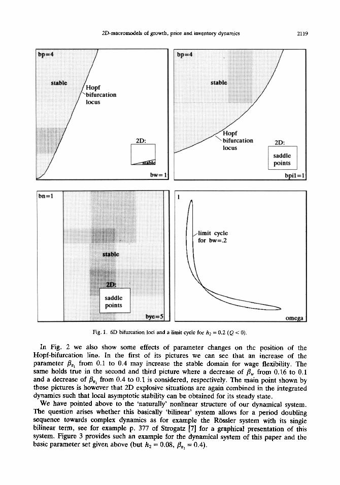
Corresponding to the three subdynamics considered in the preceding section, here we look at the stabilizing or destabilizing role of the pairs of adjustment speeds p,,,, BP, &,,, p, and &., Pn (denoted by bp, etc. in the following figures). The shaded areas in the following figures show the parameter domain where the 6D dynamics is locally asymptotically stable. The boundary of these domains is the Hopf-bifurcation locus where the system


loses -its local asymptotic St either by way-of a so-called supercritical Hopf bifurcation (where a stable-limit cycle. is b&i sfter -the .boundary has been crossed)--& by way of a subcritical Hopf bifurcat&n (where an unstable limit cycle is shrinking to ‘zero’ when the boundary is. approached). Along the bifurc&ion line there also -exist degenerate Hopf bifurcations se$&t%ting .supercritical from subcti~ical bifu&ations (where there are no iimit cycles-existing to the left and to the right of this boundary). See Wiggins 16) .for the details and graphical represemations of such &pf bi&rcations. We have found in many numerical investig&tions of the modeI that the bifurcations in the f@Iowing diagrams are generally of a supercritical~ nature.- The only important .exception is the bifurcation line on the right- hand side of the &, 8, parameter-space where the system ag&n loses stability (at & = 4:82) for hiih adjustment speeds of the parameter &. Note here also that this figure shows the independence of the domain of stability from the state. variable v and the parameter /In.

PRCWOSITION~. With respect to the above choice of parameter values the following holds: The steady-state of the dynamics (22)-(27) is. locally asymptotically stable for a high adjustment speed of prices; a low adjustment speed of wages, a low adjustnient speed -of inflationary expectations and all inventory adjustment speeds. The adjustment speed of sales expectations, by contrast, must be in the interval (0.98, 4.82), i.e. it should be neither too high nor too low.

The corresponding situation of three 2D. subdynamics is shown in the small squares in the figures. -We can see that the combination of an explosive real cycle with (unstable) saddlepoint situations i-n the monetary and.the inventory subsystem gives rise to asymptotic stability in the integrated 6D system. Note here that .there are no perverse Keynes-effects Y; > 0 or Mundell-effects Y f < 0 with respect .to the aggregate demand function of the 6D system-in contrast to the corresponding 2D situation. Furthermore:

PROPOSITION 7. With respect to the above choice of parameter values the following holds: The stabilizing properties of price and wage adjustment in the 6D system are just the opposite of those suggested by the disintegrated real cycle model.

The partial model thus gives the wrong information concerning an important policy issue, the adequate degree of wage flexibility for economic stability, Sluggish wages are now good for economic stability, while flexible wages are not. With respect to the parameter pw the bifurcation -point where local stability gets lost is approximately given by 0: = 0.16. The final picture in Fig. 1 shows the project& onto the w, I plane of stable limit cycle that is generated beyond this point at pw = 0.2. This limit cycle increases considerably in amph- tude when this parameter is increased towards /?,+ = 0.3. Thereafter the dynamics becomes purely explosive.

In Fig. 1 we have considered an example of the situation where the monetary 2D dynamics is of saddlepoint type (Q < 0). In the opposite case (Q > 0) the 2D situation also exhibits a Nopf-bifurcation line (see Proposition 2) which is shown in the small square in the following -figure (the situation for the other 2D dynamics has remained unchanged). Ignoring the very small adjustment speed in the price level the 6D dynamics has not changed very much qualitatively by the assumption of a parameter value for h2 that gives rise to Q > 0. Yet, the domain of stability is quantitatively seen significantly increased with respect to &, & by the possibility of stability for the monetary subdynamics. Note .that price fIexibility (starting. from an unstable steady state) can bring back stability to the 6D dynamics, but not to the 2D dynamics of the monetary subsystem.


bw= 1

Fig. 1. 6D bifurcation loci and a limit cycle for h2 = 0.2 (Q < 0).

In Fig. 2 we also show some effects of parameter changes on the position of the Hopf-bifurcation line. In the first of its pictures we can see that an increase of the parameter & from 0.1 to 0.4 may increase the stable domain for wage flexibility. The same holds true in the second and third picture where a decrease of /3,,, from 0.16 to 0.1 and a decrease of /3=, from 0.4 to 0.1 is considered, respectively. The main point shown by these pictures is however that 2D explosive situations are again combined in the integrated dynamics such that local asymptotic stability can be obtained for its steady state.

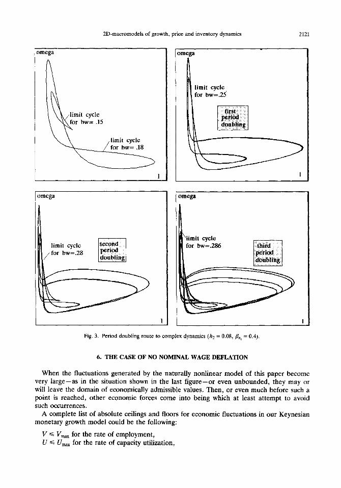
We have pointed above to the ‘naturally’ nonlinear structure of our dynamical system. The question arises whether this basically ‘bilinear’ system allows for a period doubling sequence towards complex dynamics as for example the Riissler system with its single bilinear term, see for example p. 377 of Strogatz [7] for a graphical presentation of this system. Figure 3 provides such an example for the dynamical system of this paper and the basic parameter set given above (but h2 = 0.08, /I,, = 0.4).

C. CHIARELLA and P. FLASCHEL

2D: -... -_---._/

i

insta bility

ir

,_;.:: ..: ,’ ,, j:. : t :,:: .> :’ :: II .: : /-

omega

n

Fig. 2. hD bifurcation loci and a limit cycle for h2 = 0.08

Figure 4 shows the kind of attractor that may be generated by such a sequence of .period doubling bifurcations of the limit cycle obtained by varying the bifurcation parameter &. Note that all these figures represent projections of the dynamics that is taking place in 6D phase space.

These numerical simulations also show that the cycle generated in this way becomes larger and larger and by no means stays in an economically meaningful subset of the phase space. Increasing the parameter further than shown above will also destroy mathematical boundedness. From an economic point of view it is thus clear that additional forces must come into being when certain ceilings or floors are approached with respect to quantity or value magnitudes. This is the topic of the following section.


omega

n

~~

/limit cycle for bw= .15

omega

limit cycle

/ for bw=.28

omega

I\

4 limit cycle for bw=.23

omega

limit cycle for bw=.286

Fig. 3. Period doubling route to complex dynamics (hz = 0.08, &,, = 0.4).

6. THE CASE OF NO NOMINAL WAGE DEFLATION

When the fluctuations generated by the naturally nonlinear model of this paper become very large-as in the situation shown in the last figure-or even unbounded, they may or will leave the domain of economically admissible values. Then, or even much before such a point is reached, other economic forces come into being which at least attempt to avoid such occurrences.

A complete list of absolute ceilings and floors for economic fluctuations in our Keynesian monetary growth model could be the following:

V c V,,, for the rate of employment, U s U,,,,, for the rate of capacity utilization,

(‘. CHIARELLA and P. FLASCHEL

The attracting set

Fig. 4. At the edge of mathematical houndedness ( hZ = 0.08, [jr - 0.4).

v s 0 for inventory holdings, 1 2% - h K for net investment (gross investment I -+ tiK 3 0). J’ -k 0 for the nominal rate of interest. (1) a:: r for real wages (11 and labor productivity x’.

The first two items state that there are two constraints for the output of firms at each point in time t. one (Y ,&,, z= U,,,,yPK) determined by the size of the capita1 stock which is in existence in r and which describes the maximum usage to which the physical means of production can be put (y@K the normal usage). and one (Y f;;,, I= V,,xL) which describes the maximum of labor effort available from a given labor force L (XL the normal usage). The output that is actually produced at each moment of time is thus given by

Y = min{ Y’ i 9, Y&;,,, Y&,}.

This equation should be used in the place of eqn (16) when such limits are approached. It can however be expected that the behavior of the economy changes significantly before such limits are reached.

The third of the above items states that inventories cannot become negative, It is not so binding as it appears at first sight, since unfilled orders can-and are in fact treated-as negative inventories in the present model (they are subsequently served on a first come first served basis until inventories become positive again). The fourth item is also not as


binding as it looks at first sight, since the depreciation rate may become endogenous in times of crisis where gross investment approaches zero. These items are all quantity constraints, while the last two items represent price or value constraints. Negative nominal rates of interest r will not come about due to the behavior of asset markets if this floor is approached. Finally, the mechanism that keeps real wages o below labor productivity x is not so obvious and has been controversial throughout the history of economic theory.

Of course, prices p, w as well as the capital stock K have to stay positive also, but this is assured by the formulation of their dynamics in terms of rates of growth. The above listed barriers-when approached -demand the integration of various types of nonlinearities (or additional reaction patterns such as overtime work, changes in the participation rate and immigration in the case of the full employment barrier) that may often prevent the described bound from actually being reached (and thus the Keynesian effective demand regime is left).

Astonishingly, however, all of the above additions to our demand constrained Keynesian model of monetary growth can be bypassed in many circumstances when one simple fact of modem economies is taken into account and added to the model, i.e. the nonexistence of an economy wide wage deflation is < 0. In an inflationary economy workers may demand very small nominal wage increases in the face of high unemployment, i.e. they may not attempt to resist real wage decreases when they occur in this way. By contrast, the resistance to nominal wage decreases may be formidable due to the institutional structure of the economy. Such and further related arguments have been put forth in a pronounced way by Keynes [8] in particular and they here provide the basis for the following simple modification of the money wage Phillips curve (19):

I$ = min{/?,,,(V - 1) + ~,,,j? + (1 - ~,,,)?r, O}.

This modified wage equation which excludes the occurrence of a nominal wage deflation has dramatic consequences for the stability and the pattern of fluctuations that are generated by the corresponding revised model. This will be demonstrated here by a series of simulations of this new model which create economically meaningful trajectories for all relevant variables despite pronounced increases in the formerly rapidly destabilizing adjustment parameter &.

Let us briefly describe how the model of Sections 2 and 3 is modified by oui reformulation of the money wage Phillips curve. The wage and price adjustment equations of these sections can be represented in the form

i?’ - Tf = &(v - 1) + K,(? - ?i-),

jj - 71 = &(u - 1) + Kp(@ - 77),

which gives rise to the following expressions for @ - n and fi - p:

is - ii- = K[@,(V - 1) + K,&,( u - I)], (39)

fi - %’ = K[K&,,(V - 1) + ,6,(u - I)]. (40) The simultaneous determination of wage and price deflation is thereby solved and shows that both inflation rates depend on the state of excess demand in both the market for labor and for goods and on expected medium run inflation. Subtracting the second from the first equation then gives the law of motion of the real wage we have employed in Section 3. Yet, when the rule of downwardly rigid nominal wages applies, i.e. in the case where

f@‘w(V - 1) + Kw&<u - I)] + ~7 < 0,

we have


and thus get for the real wage dynamics in this case

i3 = -&,(u - 1) - (1 - Kp)77. (41) This is the modification to be made to eqn (22) whenever the above inequality holds true. Furthermore, both eqns (24), (25) make use of the expression

jj - ?7 = K[K&(V - t) + &(u - I)1

which in the case of the above inequality must be replaced by

@ - 77 - @,(u - 1) - K,,77. (42) This completes the set of changes induced by the assumption of downwardly rigid nominal wages.

Let us now look at the consequences of this simple modification of the model. A first example is provided by Fig. 5. This figure is based on the data of Fig. 4 (p= n, i.e. no steady-state inflation in particular and also h, = 0.08, ,!$, = 0.4) and differs from the model of that figure only by the above extension of the Phillips curve. In this case the revision of the model has two basic consequences:

l The steady-state of the model is now (for p = n) no longer uniquely determined in the interior of the phase space as far as the rate of employment V,, (and lo) are concerned. Tbe rate V,, may now be lower than ‘1’ in the steady-state, since the wage

Keynes-Metzler 6D model with wage floor Keynes-Metzler 6D model with wage floor

0.500

0.492 x

.i g 0.484 f .m

B o.476

3 0.468

0.460 -0.010 1.02 1.04 1.06 1.08 1.10 1.12 1.14 1.16 1.18 0.094 0.096 0.098 0.100 0.102 0.104 0.106

-0.006

Real wage Real balances

Keynes-Metzler 6D model with wage floor Keynes-Metzler 6D model with wage floor 0.24 0.024 n77’ Y k--- ‘.. 1 -r;l I “ . I _

0.22

8 0.21

‘g 0.20,

2 0.19

g 0.18

-

0.17

0.16

0.15 ~ 0.96 0.97 0.98 0.99 1.00

‘\. _I \/ ,/ ‘\ s c .g .9 $ 0.020 0.016 0.012 0.008

i3

~ j

'i

_ /I /' 0.004 I

Y, 0.000

.Ol 1.02 1.03 0 20 40 60 80 100 120 - 140

Expected sates Time

Fig. 5. No steady-state inflation (/I 7 n = 0.05. /I,, ~~0.292 as in Fig. 4)


deflation then implied is prevented by the above change in the wage adjustment mechanism of the model (all other steady values are the same as before).

l The set of steady-states of the revised model is now globally asymptotically stable in a very strong way (see Fig. 5 for an example). Due to the changed behavior of workers the economy is rapidly trapped in an underemployment equilibrium that may be much higher than the NAIRU rate of unemployment of the former steady-state situation.

We thus have that downward wage rigidity prevents the fluctuations shown in Fig. 4 in a radical way, but is accompanied by a more depressed labor market in the steady-state than before. These results are in our view due to the fact that there is a floor or ratchet built into the model right at the edge of the steady-state.

This observation suggests that there will be more fluctuations if there is steady-state inflation, i.e. if p > n is assumed, since the behavior of the economy is then only modified further away from the steady-state which in this case is again uniquely determined as in the preceding model. Locally it is thus of the form of the preceding section. The interesting question then is whether the dynamics is again radically modified by the ratchet situation that the level of nominal wages may rise, but cannot fall. Figures 6-12 illustrate this for a wage adjustment speed /Iw, that varies from 2 to 26, i.e. over a range where the previous model would collapse immediately.

This series of figures shows that the period doubling route to complex dynamics shown in Figs 3 and 4 can also be demonstrated to exist in this model variant, but now for extremely

Keynes-Metzler 6D model with wage floor Keynes-Metzler 6D model with wage floor

0.80 1 0.75

0.70 0.65 .

0.60 0.55 0.50

0.45 0.40

. 0.8 0.9 1.0 1.1 1.2 1.3 1.4

Real wage

0.12

o.la

0.08

0.06

0.04

, . . . . . .m I 0.080 0.090 0.100 0.110 0.120

Real balances

Keynes-Metzler 6D model with wage floor Keynes-Metzler 6D model with wage floor r 0.36

0.32 0.28

0.05 I - I L LL 0.88 0.92 0.96 1.00

0.00 1.04 1.08 1.12 1.16 1.20 0 20 40 60 80 100 120 140 160 180 200

Expected sales Time

Fig. 6. Steady-state inflation (y = 0.1 z n = 0.05) and period-l limit cycles (pW = 2).

2126 C. CWIARELLA and P. FLASCHEL

Keynes-Mctxkr 5p model with wage floor 0.90

Keynes-Metzler 6D model with wage floor 0.14

0.80 0 ii 0.12

h .f: 0.10 a 0.70

2 *m

Y z 0.08

i 0.60 c .4

‘5: -1 ij

0.04 0.06

0.50 tit LG 0.02

0.40 0.00 0.8 0.9 1.0 1.1 1.2 1.3 1.4 1.5 1.6 0.06 0.07 0.08 0.09 0.10 0.11 0,12 0.13

Real wage Real balances

Keyrtcs-Walzlcr 6D modei with wage floor 0.6 1 1

0.5

0.1

0.0 0

Keynes-Metzlcr 6D model with wage floor

0 20 40 60 80 100 120 140 160 180 200 Expected sales Time

Fig. 7. Steady-state inflation and period-2 limit cycles (&, = 5).

high adjustment speeds /?,+ of nominal wages w and amplitudes of fluctuations that stay within economically meaningful bounds. Note that wage inflation can get as high as 130% and that inventories may become slightly negative in the Fig. 12 where the case /3, = 26 is considered.

Figures 6-12 each show three projections of the 6D dynamics onto the w, I, the rn, -r and the y’, Y subspace as well as the development of wage inflation as a time series. This series of figures demonstrates several things:

l The model is now extremely viable, but, as expected, no longer asymptotically stable. l The model exhibits large but economically meaningful persistent fluctuations. o The model undergoes a period doubling sequence as the parameter pn, is increased

further and further. l The model shows only weak changes in amplitude while the parameter /?,,, is increased

significantly. l The economic length of the cycle stays approximately 20 years, while the mathematical

period of course doubles along the period doubling route.

The dynamics therefore eventually becomes complex as the parameter pW is increased further and further. This is also suggested by the bifurcation diagrams’shown in Figs 13 and


Keynes-Metzler 6D model with wage floor

0.9

2 0.8

i 0.1

g 0.6

3 0.5

0.6 0.8 1.0 1.2 1.4 1.6 1.8

Real wage

0.6 Keynes-Metzler 6D model with wage floor

0.85 0.90 0.95 1.00 1.05 1.10 1.15, 1.20 1.25

Expected sales


2 0.14

5 '", 0.10

F ; 0.06 ?z! :: 2

0.02

u -0.02

0.06 0.07 0.08 0.09 0.10 0.11 0.12 0.13

Real balances

Keynes-Metzler 6D model with wage floor 0.7,...................,

0.6

E 0.5 .s d G

0.4

.f! 0.3 I% a is 0.2

0.1

0.0 0 1002003004005006007008009001000

Time

Fig. 8. Steady-state inflation and period-4 limit cycles (/SW = 10).

14, which plot the local maxima of the state variable w on the attracting set for values of the parameter /3,,, in the interval [15, 301. The dynamics of the naturally nonlinear model is thus radically changed from a global perspective, though not from a local perspective, where the earlier Hopf-bifurcation analysis of this paper still applies.

7. CONCLUDING REMARKS

In Keynes [4] it is stated: “Thus it is fortunate that workers, though unconsciously, are instinctively more reasonable economists than the classical school, inasmuch as they resist reductions of money-wages, which are seldom or never of an all-round character . . .” (p. 14) and “The chief result of this policy (of flexible wages, C.C./P.F.) would be to cause a great instability of prices, so violent perhaps as to make business calculations futile . . .” (p. 269). The present Keynesian model of monetary growth has demonstrated the validity of this view by means of numerical simulations of a system of laws of motion of considerable completeness and complexity. Of course, other sources for stability may also exist, but must be left for future research.

212H C. CHIARELLA and P. FLASCHEI.

Keynes-Metzltr 6D model with wage floor I .o

0.9

3 0.8 ii ‘i 0.7

jj 0.6

el 0.5

I . .

0.6 0.8 1.0 1.2 1.4 1.6 1.8

Real wage

Ktynes-kgaukr 6D model with wage floor

-.- 0.85 0.90 0.95 1.00 1.05 1.10 I.15 1.20 1.25

Expected sales


0.06 0.07 0.08 0.09 0.10 0.11 0.12 0.13

Real balances

Keynes-Metzfer 6D model with wage floor 0.8, _ 1

0.7

0.6 E ‘$ 0.5

g. 0.4

& 0.3

g 0.2

0.1

Time

300 350 1111 f Do 450 00

Fig. 9 Steady-state inflation and period-8 limit cycles C/5., = 10.7)

ZD-macromodels of growth, price and inventory dynamics 2129


.g 0.8

E E 0.7 .I

5 0.6

3 0.5

0.4 0.6 0.8 1.0 1.2 1.4 1.6 1.8

Real wage


0.5

; 0.4 'cl 9 0.3 5 i 0.2

0.1

0.0 1 J 0.85 0.90 0.95 1.00 1.05 1.10 1.15 1.20 1.25

Expected sales

Keynes-Metzler 6D model with wage floor 0.18 , 7F I

L 9)

5 0.14

E '2 0.08 c 2 0.06 0 t g 0.02 .

2 m -0.02- - .

0.06 0.07 0.08 0.09 0.10 0.11 0.12 0.13

Real balances


I

o 50 1001502002!

Time

Fig. 10. Steady-state inflation and period-16 limit cycles (fiW = 11).




71

2-l 0.9’ .z 2 2 0.8 .

2 0.7

4 0.61. 4

0.5:. wl 0.4 ’

0.6 0.8 1.0 1.2 1.4 1.6 1.8

Real wage

Keynes-Mdtzfer 6D modal with wage floor 0.7, . I

0.6 .’ t

0.85 WOO.95 1.00 1.05 1.10 1.1s 1.20 1.25 1.30

Expected sales

0.06 0.07 0.08 0.09 0.10 0.11 0.12 0.13

Real balances

Keynes-kktzler 6D model with wage floor

0.7

OId 8 ‘S 0.5

2 2 0.4

& 0.3

g 0.2

0.1 0.0

0 100 -200 300 400 so0 600 780 800 900 1000

Time

Fig. 1 I. Steady-state inflation and period n? (p,, = 13)


Keynes-Metzler 6D model with wage floor 1.8, I

1.6

0.4 0.4 0.6 0.8 1.0 1.2 1.4 1.6 1.8 2.0

Real wage

Keynes-Metzler 6D model with wage floor Keynes-Metzler 6D model with wage floor 1 .o

0.8

2 0.6 ‘i: ,o 0.4 8 :: 0.2

0.0

-0.2

V

Y,

0.7 0.8 0.9 1.0 1.1 1.2 1.3 1.4

Expected sales

1.5


0 F?

0.18

E 0.14

a 0.10 G. .E 0.06 B g 0.02 tit K -0.02 w -0.06 1 ,IZ .

0.04 0.06 0.08 0.10 0.12 0.14

Real balances

1.4r,, . . .

E 1.0 2 a 0.8 c -5 0.6 & * 8 0.A

0.2:

0.0 0 400 800 1200 I600 2000

Time

Fig. 12. Steady-state inflation and complex dynamics (BW = 26).


1.61

1 s2

F.‘~‘~..‘*~....l~.‘.~“.‘l”...“*‘~~~”~~ 13.5 15.8 18.0 20.2 22.5 24.7 27.0 29.2 31.5

Fig. t3. A bifurcation diagram for the parameter /jw and the state variable m.

LA-” “1,’ a’>’ I,,,,l~,,‘l,,,,i,,,,I,,,,

13.6 15.8 18.0 20.3 22.5 24.7 27.0 29.2 31.4

Fig. 14. Zooming onto the middle section of the bifurcation diagram.


REFERENCES

1. C. Chiarella and P. Flaschel, A complete Keynesian model of monetary growth with sluggish price and quantity adjustments. Discussion paper, University of Bielefeld (1995).

2. C. Chiarella and P. Flaschel, Descriptive monetary macrodynamics: Foundations and extensions. Draft manu- script, Department of Economics, University of Bielefeld (1995).

3. H. Rose, On the non-linear theory of the employment cycle. Rev. Econ. Stud. XXXIV(!B), 153-173 (1967). 4. P. Cagan, The monetary dynamics of hyperinflation. In Studies in the Quantity Theory of Money, edited by

M. Friedman. University of Chicago Press (1956). 5. L. Metxler, The nature and stability of inventory cycles. Rev. Econ. Stat. 23, 113-129 (1941). 6. S. Wiggins, Introduction to Applied Nonlinear Dynamical Systems and Chaos. Springer-Verlag, New York

7. S. Strogatz, Nonlinear Dynamics and Chaos. Addison-Wesley, Reading, MA (1994). 8. J. M. Keynes, The General Theory of Employment, Interest and Money. Macmillan, New York (1936).

Documents

An integrative approach to 2D-macromodels of growth, price and inventory dynamics