Embed Size (px)
Citation preview

Scholars' Mine Scholars' Mine
Masters Theses Student Theses and Dissertations
Spring 2018
An integrated method for understanding the fluid flow behavior An integrated method for understanding the fluid flow behavior
and forecasting well deliverability in gas condensate reservoirs and forecasting well deliverability in gas condensate reservoirs
with water aquifer drive with water aquifer drive
Abdulaziz Mustafa Em. Ellafi
Follow this and additional works at: https://scholarsmine.mst.edu/masters_theses
Part of the Petroleum Engineering Commons
Department: Department:
Recommended Citation Recommended Citation Ellafi, Abdulaziz Mustafa Em., "An integrated method for understanding the fluid flow behavior and forecasting well deliverability in gas condensate reservoirs with water aquifer drive" (2018). Masters Theses. 7760. https://scholarsmine.mst.edu/masters_theses/7760
This thesis is brought to you by Scholars' Mine, a service of the Missouri S&T Library and Learning Resources. This work is protected by U. S. Copyright Law. Unauthorized use including reproduction for redistribution requires the permission of the copyright holder. For more information, please contact [email protected].

i
AN INTEGRATED METHOD FOR UNDERSTANDING THE FLUID FLOW
BEHAVOIR AND FORECASTING WELL DELIVERABILITY IN GAS
CONDENSATE RESERVOIRS WITH WATER AQUIFER DRIVE
by
ABDULAZIZ MUSTAFA EM. ELLAFI
A THESIS
Presented to the Faculty of the Graduate School of the
MISSOURI UNIVERSITY OF SCIENCE AND TECHNOLOGY
In Partial Fulfillment of the Requirements for the Degree
MASTER OF SCIENCE IN PETROLEUM ENGINEERING
2018
Approved by
Ralph Flori, Advisor Shari Dunn-Norman
Mingzhen Wei

ii
2018
Abdulaziz Mustafa Em.Ellafi
All Rights Reserved

iii
ABSTRACT
Gas condensate reservoirs constitute a significant portion of global hydrocarbon
reserves. In these reservoirs, as bottomhole pressure falls below the dew point, liquid
develops in the pore space. This results in the formation of a liquid bank near the wellbore
region that decreases gas mobility, which then reduces gas inflow. Some gas condensate
reservoirs have bottom aquifer drive, which also negatively impacts gas production. This
research used a field case study to demonstrate an integrated workflow for forecasting well
deliverability in a gas condensate field in Libya. The workflow began with the
interpretation of open-hole log data to identify the production interval net pay and to
estimate petrophysical properties. A compositional model was developed and matched to
actual reservoir fluids. Transient pressure analysis was described and used to identify
reservoir properties. Inflow performance relationships (IPRs) were analyzed using three
types of backpressure equations. The workflow integrated all data in a numerical
simulation model, which included the effect of bottom water drive. Sensitivity analysis was
used to identify parameters with the greatest impact on future deliverability and recovery.
The results provided in this case study demonstrated the importance of an integrated
workflow in predicting future well performance in gas condensate fields with bottom water
drive. The study demonstrated how to implement the workflow in managing or developing
these types of reservoirs.

iv
ACKNOWLEDGMENTS
First, I would like to thank Allah for giving me the strength, knowledge, ability,
and opportunity to accomplish this research.
I would like to express my sincere gratitude to my advisor, Dr. Ralph Flori who,
has been a great teacher, a friend, an inspiration, a role model and a pillar of support in my
guide.
I am thankful for the members of my advisory committee: Dr. Shari Dunn-Norman
for her technical guidance and Dr. Mingzhen Wei for her continuous assistance.
I am grateful to the Libyan Ministry of Education for the financial support during
my academic study. I also wish to acknowledge Mellitah Oil & Gas B.V. for providing me
with all the field data needed to complete this research.
I highly appreciate Mr. Ole S. Fjaere (Kappa Engineering Technical Support), Dr.
Mohsen Khazam (University of Tripoli), Prof. Thomas A. Blasingame (Texas A&M), Prof.
John Spivey (Phoenix Reservoir Engineering), and Ms. Emily Seals (Missouri S&T) for
their valuable explanation and guidance.
My acknowledgement would be incomplete without thanking the biggest source of
my strength, my family. This would not have been possible without their unwavering and
unselfish love and support given to me at all times.

v
TABLE OF CONTENTS
Page
ABSTRACT ....................................................................................................................... iii
ACKNOWLEDGMENTS ................................................................................................. iv
LIST OF FIGURES ............................................................................................................ x
LIST OF TABLES .......................................................................................................... xvii
SECTION
1. INTRODUCTION ..................................................................................................... 1
1.1 SIGNIFICANCE OF GAS CONDENSATE IN GAS PRODUCTION .............. 1
1.1.1 Gas Condensate Phase and Fluid Flow Behavior. ........................................ 2
1.1.2 Water Influx Gas Condensate. ...................................................................... 4
1.2 PRESSURE TRANSIENT ANALYSIS .............................................................. 5
1.2.1 Drawdown Test. ........................................................................................... 7
1.2.2 Buildup Test. ................................................................................................ 7
1.3 FLOW REGIME CATEGORIES ........................................................................ 8
1.3.1 Steady-state Flow. ........................................................................................ 8
1.3.2 Pseudo-steady State Flow. ............................................................................ 9
1.3.3 Unsteady State Flow. .................................................................................. 10
1.4 WELL DELIVERABILITY ............................................................................... 12
1.5 MODELING OF COMPOSITIONAL SIMULATION ..................................... 14
1.6 RESERVOIR SIMULATION ............................................................................ 15

vi
1.7 OVERVIEW OF THE NORTH AFRICAN FIELD .......................................... 17
1.8 RESEARCH OBJECTIVES .............................................................................. 18
1.9 RESEARCH SCOPE ......................................................................................... 20
2. LITERATURE REVIEW ........................................................................................ 21
2.1 GAS CONDENSATE CHARACTERIZATION ............................................... 21
2.2 GAS CONDENSATE FLOW BEHAVIOR ...................................................... 25
2.3 HISTORY OF GAS WELLS DELIVERABILITY ........................................... 27
2.4 INFLUENCE OF WATER AQUIFER SUPPORT ........................................... 32
3. METHODOLOGY .................................................................................................. 34
3.1 OPEN-HOLE LOGS INTERPRETATION ....................................................... 34
3.1.1 Wireline Logging Tools. ............................................................................ 35
3.1.1.1 Lithology logs. ..................................................................................... 36
3.1.1.2 Porosity logs. ....................................................................................... 36
3.1.1.3 Resistivity logs. ................................................................................... 37
3.1.2 Interpretation Procedures. .......................................................................... 38
3.2 COMPOSITIONAL SIMULATION (PHASE BEHAVIOR) ........................... 43
3.3 RESERVOIR GAS CONDENSATE PROPERTIES ........................................ 47
3.3.1 Gas Deviation Factor. ................................................................................. 47
3.3.2 Gas Viscosity. ............................................................................................. 52
3.3.3 Isothermal Compressibility. ....................................................................... 53

vii
3.4 GAS WELL TESTING INTERPRETATION ................................................... 54
3.4.1 Pressure Derivative Plot. ............................................................................ 55
3.4.1.1 Single-phase pseudo-pressure.............................................................. 55
3.4.1.2 Adjusted pressure. ............................................................................... 56
3.4.1.3 Pseudo-time and adjusted time. ........................................................... 57
3.4.1.4 Superposition in time. .......................................................................... 57
3.4.1.5 The Bourdet derivative. ....................................................................... 58
3.4.2 Type Curve Analysis. ................................................................................. 60
3.4.3 Interpretation procedures. ........................................................................... 61
3.4.4 Pressure Derivative and Superposition Plot. .............................................. 64
3.4.4.1 Gringarten type curve. ......................................................................... 66
3.4.4.2 Kappa Saphir software. ........................................................................ 69
3.5 WELL DELIVERABILITY ............................................................................... 75
3.5.1 Excel Sheet Calculation. ............................................................................. 76
3.5.2 Prosper Software. ....................................................................................... 82
3.6 RESERVOIR SIMULATION ............................................................................ 85
3.6.1 Simulation Model Description. .................................................................. 86
3.6.2 Reservoir Rock Properties. ......................................................................... 86
3.6.3 Reservoir Fluid Properties (PVT data). ...................................................... 87
3.6.4 Special Core Analysis Data (SCAL data). ................................................. 87
3.6.5 Initial Conditions. ....................................................................................... 89
3.6.6 Wells and Recurrent Section. ..................................................................... 89

viii
3.6.7 Numerical Section. ..................................................................................... 90
3.6.8 Water Aquifer Properties. ........................................................................... 90
3.6.9 Reservoir Pressure History. ........................................................................ 91
3.6.10 Gas, Condensate, and Water Production History. ...................................... 91
3.6.11 Future Performance. ................................................................................... 91
3.7 SENSITIVITY ANALYSIS ............................................................................... 92
3.7.1 Completion Perforation. ............................................................................. 92
3.7.2 Volume Lift Pressure Curve (VLP). ........................................................... 93
4. RESULTS AND DISCUSSION .............................................................................. 94
4.1 FORMATION EVALUATION OF THE FIELD .............................................. 94
4.2 FLUID CHARACTERISTICS OF THE FIELD ............................................... 96
4.3 COMPATIBLE GAS PROPERTIES CORRELATIONS OF THE FIELD .... 100
4.3.1 Gas Deviation Factor. ............................................................................... 100
4.3.2 Gas Viscosity. ........................................................................................... 102
4.3.3 Isothermal Compressibility. ..................................................................... 102
4.3.4 Pseudo-Gas Potential Pressure. ................................................................ 103
4.4 RESERVOIR CHARACTERISTICS OF THE FIELD ................................... 106
4.4.1 Analytical Method Results. ...................................................................... 106
4.4.2 Type Curve Results. ................................................................................. 109
4.4.3 Modern Method Results. .......................................................................... 110
4.4.4 Dependent Skin Results. ........................................................................... 113

ix
4.4.5 Comparison Between Two Tests. ............................................................. 116
4.5 THE FIELD FLOW POTENTINAL................................................................ 116
4.5.1 Analytical Results. .................................................................................... 116
4.5.2 Explanation of Results. ............................................................................. 123
4.5.3 Comparison between Two Tests. ............................................................. 126
4.6 SIMULATION OUTCOMES OF THE FIELD ............................................... 129
4.7 FUTURE FLOW PERFORMANCE OF THE FIELD .................................... 136
4.7.1 Applicability of Equations. ....................................................................... 136
4.7.2 Application of the Equations. ................................................................... 137
4.7.3 Future Scenarios for Matching VLP with IPR. ........................................ 139
4.8 DEVELOPMENT STRATEGY PLAN OF THE FIELD ................................ 141
5. CONCLUSIONS & RECOMMENDATIONS ...................................................... 145
5.1 CONCLUSIONS .............................................................................................. 145
5.2 FUTURE WORK RECOMMENDED ............................................................. 149
BIBLIOGRAPHY ...................................................................................................... 150
VITA .......................................................................................................................... 157
x
LIST OF FIGURES
Page
Figure1.1. A typical gas condensate phase envelope (Zendehboudi et al., 2012). ............. 3
Figure1.2. Drawdown test (modified from Spivey et al., 2013). ........................................ 7
Figure1.3. Buildup test (modified from Spivey et al., 2013). ............................................. 7
Figure1.4. Steady-state flow plot for buildup test/drawdown test (modified from Fekete Associates Inc, 2010). ....................................................................................... 8
Figure1.5. Pseudo-steady state flow plot for drawdown test (modified from Fekete
Associates Inc, 2010). ..................................................................................... 9 Figure 1.6. Pseudo-steady state flow plot for builduptest (modified from Fekete
Associates Inc, 2010). ................................................................................... 10 Figure 1.7. Unsteady state flow plot for buildup test/drawdown test (modified from
Fekete Associates Inc, 2010). ........................................................................ 11 Figure 1.8. Plot of pressure versus time for all regimes (modified from Fekete Associates
Inc, 2010). .................................................................................................... 11 Figure 1.9. The pressure derivative plot for all regimes (modified from Fekete Associates
Inc, 2010). .................................................................................................... 12 Figure 1.10. Flow-after-flow test. ..................................................................................... 13
Figure 1.11. Liquid dropout curve at 220˚F for binary gas condensate system (modified from Whitson et al., 2005). .......................................................................... 15
Figure 1.12. Flowchart for research scope. ....................................................................... 20
Figure 2.1.Ternary visualization of hydrocarbon classification (Whitson et al., 2000). .. 22
Figure 2.2. Phase diagram of a gas-condensate system (Fan et al., 2006). ....................... 23
Figure 2.3. Phase diagram of a lean and rich gas condensate system (Fan et al., 2006). . 24
Figure 2.4. Liquid dropout for a lean and rich gas condensate system (Fan et al., 2006). 24

xi
Figure 2.5. Change in condensate saturation and gas throughout reservoir (modified from Roussennac, 2001). ......................................................................................... 26
Figure 2.6. Typical flow-after-flow test. ........................................................................... 28
Figure 2.7. Reverse sequence of flow-after-flow test. ...................................................... 28
Figure 2.8. Typical isochronal test. ................................................................................... 30
Figure 3.1. Formation evaluation open-hole logs data. .................................................... 35
Figure 3.2. Schlumberger’s chart (Gen-9) to estimate formation water resistivity (Schlumberger, 2013). ................................................................................... 40
Figure 3.3. The target formation open-hole logs. ............................................................. 41
Figure 3.4. The hydrocarbon and non-hydrocarbon series. .............................................. 44
Figure 3.5. Phase envelope for the gas condensate system before reaching the match using EOS. ..................................................................................................... 44
Figure 3.6. Phase envelope for gas condensate system after reaching the match using
EOS. .............................................................................................................. 45 Figure 3.7. Regression process to tune the reservoir fluid. ............................................... 46
Figure 3.8. Multi-rate flow profile and pressure response due to different rates (modified from Liang et al., 2013). ................................................................................. 58
Figure 3.9. Bourdet derivative, semi-log and log-log (Dynamic Flow Analysis, Kappa,
2012). .............................................................................................................. 59 Figure 3.10. Schematic of Bourdet derivative algorithm (Dynamic Flow Analysis, Kappa,
2012). .............................................................................................................. 60 Figure 3.11. Gringarten and Bourdet type curve (Gringarten et al., 1979)....................... 61
Figure 3.12. Derivative overlay for four drawdowns before adjusted flow rates. ............ 63
Figure 3.13. Derivative overlay for four drawdowns after adjusted flow rates. ............... 63
Figure 3.14. Pressure derivative plot for buildup test. ...................................................... 64

xii
Figure 3.15. Radial flow regions on the pressure derivative plot. .................................... 64
Figure 3.16. Gringarten type curve for the first radial flow region. ................................. 66
Figure 3.17. Gringarten type curve for the second radial flow region. ............................. 68
Figure 3.18. Gringarten type curve for the third radial flow region. ................................ 68
Figure 3.19. The main reservoir parameters. .................................................................... 69
Figure 3.20. PVT data. ...................................................................................................... 70
Figure 3.21. The interpretation for the first drawdown. ................................................... 71
Figure 3.22. The interpretation for the second drawdown. ............................................... 71
Figure 3.23. The interpretation for the third drawdown. .................................................. 72
Figure 3.24. The interpretation for the fourth drawdown. ................................................ 72
Figure 3.25. The interpretation for the buildup................................................................. 73
Figure 3.26. Derivative overlay for the four drawdowns. ................................................. 74
Figure 3.27. Rate-dependent skin plot. ............................................................................. 74
Figure 3.28. The history pressure before reaching the match using rate-dependent skin. 74
Figure 3.29. The history pressure after reaching the match using rate-dependent skin. ... 75
Figure 3.30. Flow-after-flow test. ..................................................................................... 76
Figure 3.31. Deliverability calculation (empirical method).............................................. 78
Figure 3.32. Deliverability calculation (empirical method).............................................. 78
Figure 3.33. Deliverability calculation (theoretical method). ........................................... 80
Figure 3.34. Deliverability calculation (Exact method).................................................... 81
Figure 3.35. Downhole equipment.................................................................................... 83
Figure 3.36. Vertical lift pressure input-data. ................................................................... 84
Figure 3.37. The vertical lift pressure system for current case. ........................................ 85

xiii
Figure 3.38. Radial reservoir simulation model description. ............................................ 86
Figure 3.39. Two-phase water-oil (condensate) relative permeability. ............................ 88
Figure 3.40. Two phase gas-oil (condensate) relative permeability. ................................ 88
Figure 3.41. Three phase gas-oil (condensate)-water relative permeability. .................... 89
Figure 4.1. The main calculations for the open-hole log interpretation............................ 95
Figure 4.2. Elan volume and Elan fluid for the well A-7. ................................................ 96
Figure 4.3. Constant volume depletion (CVD) model. ..................................................... 97
Figure 4.4. Constant composition expansion (CCE) model. ............................................ 98
Figure 4.5. Phase envelope diagram for the gas condensate reservoir with 1% liquid volume ranges between the quality lines. ...................................................... 99
Figure 4.6. Phase envelope diagram for the gas condensate reservoir with 0.1% liquid
volume ranges between the quality lines. .................................................... 100 Figure 4.7. Results of gas deviation factor using different methods. ............................. 101
Figure 4.8. Comparison between gas deviation factor from the laboratory measurements and averaging value from different methods. ............................................... 101
Figure 4.9. Relationship between gas viscosity using Lee, Gonzalez, and Eakin
correlation and pressure. .............................................................................. 102 Figure 4.10. Relationship between isothermal compressibility and pressure. ................ 103
Figure 4.11. Relationship between gas properties and pressure. .................................... 104
Figure 4.12. Relationship between pseudo-gas potential pressure and pressure. ........... 105
Figure 4.13. Relationship between adjusted pressure and pressure. ............................... 105
Figure 4.14. Pressure derivative plot for the buildup test. .............................................. 107
Figure 4.15. Superposition plot for the first radial flow regions. ................................... 107
Figure 4.16. Superposition plot for the second radial flow regions. ............................... 108

xiv
Figure 4.17. Superposition plot for the third radial flow regions. .................................. 108
Figure 4.18. Pressure derivative plot for the buildup test using standard model. ........... 111
Figure 4.19. Pressure derivative plot of the first drawdown test. ................................... 112
Figure 4.20. Pressure derivative plot of the second drawdown test................................ 112
Figure 4.21. Pressure derivative plot of the third drawdown test. .................................. 112
Figure 4.22. Pressure derivative plot of the fourth drawdown test. ................................ 113
Figure 4.23. The relationship between equivalent gas flow rate and composite radius. 113
Figure 4.24. The initial results of the rate-dependent skin method. ............................... 114
Figure 4.25. The pressure history match though the test using the rate-dependent skin method........................................................................................................ 115
Figure 4.26. The results of the rate-dependent skin method. .......................................... 115
Figure 4.27. The pressure history match though the test using the time-dependent skin method........................................................................................................ 115
Figure 4.28. The pressure derivative overlay for the buildup tests in 2009 and 2014. ... 116
Figure 4.29. Deliverability analysis using the empirical method with the Excel. .......... 117
Figure 4.30. The empirical inflow performance relationship using Prosper. ................. 118
Figure 4.31. Match of vertical lift performance with the empirical inflow performance relationship using Prosper software. .......................................................... 118
Figure 4.32. Deliverability analysis using the theoretical method with Excel. .............. 119
Figure 4.33. The theoretical inflow performance relationship using Prosper. ................ 120
Figure 4.34. Match of vertical lift performance with the theoretical inflow performance relationship using Prosper software. .......................................................... 120
Figure 4.35. Deliverability analysis using the exact method with Excel. ....................... 121
Figure 4.36. The exact inflow performance relationship using Prosper. ........................ 122

xv
Figure 4.37. Match of vertical lift performance with the exact inflow performance relationship using Prosper. ......................................................................... 122
Figure 4.38. Match of vertical lift performance with the three inflow performance
relationship methods using Prosper software. ........................................... 123 Figure 4.39. Relationship between gas properties with pressure. ................................... 124
Figure 4.40. Modified empirical equation results. .......................................................... 124
Figure 4.41. Match of vertical lift performance with the modified empirical inflow performance relationship using Prosper. .................................................... 125
Figure 4.42. Match of vertical lift performance with all methods of the inflow
performance relationship using Prosper. .................................................... 126 Figure 4.43.Empirical method calculations in 2009 and 2014. ...................................... 127
Figure 4.44. Empirical inflow performance relationship in 2009 and 2014. .................. 127
Figure 4.45. Theoretical inflow performance relationship in 2009 and 2014. ............... 128
Figure 4.46. Exact inflow performance relationship in 2009 and 2014.......................... 128
Figure 4.47. Reservoir average pressure history result using reservoir simulation. ....... 129
Figure 4.48. Relationship between reservoir average pressure and water cut simulation history. ....................................................................................................... 130
Figure 4.49. Reservoir pressure history result match with the well-testing results using
reservoir simulation. .................................................................................. 131 Figure 4.50. Gas production rate simulation history....................................................... 132
Figure 4.51. The relationship between the gas production rate and water cut simulation history. ....................................................................................................... 132
Figure 4.52. Condensate production rate simulation history. ......................................... 133
Figure 4.53. The relationship between the condensate production rate and water cut simulation history....................................................................................... 134
Figure 4.54. Condensate dropout throughout the reservoir radius.................................. 135

xvi
Figure 4.55. Condensate dropout over the years............................................................. 135
Figure 4.56. Water cut over years. .................................................................................. 135
Figure 4.57. Predicting the IPR curves using the modified empirical method. .............. 138
Figure 4.58. Predicting the IPR curves using the theoretical method. ............................ 139
Figure 4.59. Predicting the match of VLP with the empirical IPR curves. .................... 140
Figure 4.60. Predicting the match of VLP with the theoretical IPR curves.................... 140
Figure 4.61. The North African formation schematic. .................................................... 141
Figure 4.62. Water cut sensitivity results over the years. ............................................... 142
Figure 4.63. Gas production rate sensitivity results over the years. ............................... 142
Figure 4.64. Gas recovery factor sensitivity results over the years. ............................... 143

xvii
LIST OF TABLES
Page
Table 1.1. Reservoir properties obtainable from various transient tests (Kamal et al., 1995). .................................................................................................................. 6
Table 1.2. Specific flow regimes within all categories (Fekete Associates Inc, 2010). ... 12
Table 2.1. Typical Characterization for differentiate hydrocarbon type (Wall, 1982). .... 21
Table 2.2. Typical hydrocarbon composition for different fluid types (Wall, 1982). ...... 22
Table 2.3.Typical values of classification of gas condensate fluid................................... 25
Table 3.1. Sonic velocities and interval transient times for different formations (Schlumberger, 1972). ...................................................................................... 37
Table 3.2. The coefficients of Dranchuk and Abu-Kassem correlation (Ahmed, 2006). . 52
Table 3.3. The main input of the first region for the Gringarten type cure approach. ...... 67
Table 3.4. The main input of the second and third regions for the Gringarten type cure approach. ......................................................................................................... 69
Table 3.5. Main input data for the deliverability calculations. ......................................... 76
Table 3.6. Input calculation data in the empirical method. ............................................... 77
Table 3.7. Input calculation data in the theoretical method. ............................................. 79
Table 3.8. Input calculation data in the exact method. ..................................................... 81
Table 3.9. Geothermal gradient data. ................................................................................ 83
Table 3.10. Average heat capacities (Petroleum expert manual). ..................................... 83
Table 3.11. The main input data for reservoir rock properties. ........................................ 87
Table 3.12. Initial condition parameters. .......................................................................... 89
Table 3.13. Numerical default and dataset values. ........................................................... 90
Table 3.14. Data for the water aquifer properties. ............................................................ 90
xviii
Table 4.1. The results obtained from formation evaluation process. ................................ 96
Table 4.2. Well-testing interpretation results for three radial flow regions using superposition plot. ......................................................................................... 109
Table 4.3. Well-testing interpretation results for three radial flow regions using
Gringarten type curve. .................................................................................. 110 Table 4.4. The water aquifer properties data. ................................................................. 130
Table 4.5. The equation applicability in the modified empirical method. ...................... 136
Table 4.6. Relative error results for the modified empirical method calculations. ......... 136
Table 4.7. The equation applicability in the theoretical method. .................................... 137
Table 4.8. Relative error results for the theoretical method calculations. ...................... 137
Table 4.9. The prediction results of the IPR parameters................................................. 137
Table 4.10. The prediction results of the IPR parameters............................................... 138
Table 4.11. The results of the formation thickness sensitivity. ...................................... 144
Table 4.12. The final results of the formation thickness sensitivity in the target year. .. 144

1
1. INTRODUCTION
In recent years, the global demand for energy resources rapidly increased, and as
the world oil and gas reserves leveled off, production from existing reservoirs became a
greater challenge that required a better understanding of reservoir engineering basics and
developed technology applications. Awareness of such concepts plays an important role
for any reservoir study. With improvement in technology and knowledge, the achievement
of the study becomes much more efficacious. Development plans induced from any study
depend mainly on the effects of fluid behavior and reservoir parameters on well
productivity and thus the recoverable oil and gas.
Gas condensate fluids behave differently from gas and oil flow. Such distinctive
behavior needs to be observed and quantified. Simulation technology is an additional tool
for the technical measurement, which can overcome the insufficiency of the experimental
measurement. Therefore, the study of the gas condensate flow performance is still a
relevant project (Al-Shaidi et al., 1997).
1.1 SIGNIFICANCE OF GAS CONDENSATE IN GAS PRODUCTION
Gas condensate reservoirs constitute an important portion of global hydrocarbon
reserves that are economically profitable. Gas condensate reservoirs comprise more than
6,183 trillion cubic feet of the world’s gas reserves (U.S. Energy Information
Administration., 2015). The most important gas condensate reservoirs in the world that
contain huge reserves are located in the following fields: the Arun field in Indonesia, the
Shtokmanovskoye field in the Russian Barents Sea, the Karachaganak field in the

2
Kazakhstan, the offshore North field in Qatar, the South Pars field in Iran, and the
Cupoagua field in Colombia (Li et al., 2005). This research will focus on the importance
of gas condensate reservoirs in Libya. Libya has 1,504.9 billion cubic meters of proven gas
reserves, and the main gas condensate fields are distributed in the following fields: W-12,
F-12, N-8, and North African (National Oil Corporation of State of Libya).
1.1.1 Gas Condensate Phase and Fluid Flow Behavior. Considering the
reservoir conditions (pressure and temperature), Figure 1.1 shows a phase diagram of the
gas condensate system. The two-phase region is enclosed within the bubble-point line, the
dew-point line, and the critical point. The lines numbered inside the two-phase region are
called quality lines, and each represents the liquid fraction within the fluid defined at
certain reservoir conditions. For typical gas condensate reservoirs, the initial pressure is
above the cricondenbar, which refers to the maximum pressure at which the two-phase
region can exist in equilibrium. The initial reservoir temperature for a gas condensate
system lies between the critical temperature and the cricondentherm (Raghavan et al.,
1996).
The typical reservoir temperature for gas condensate reservoirs is normally 200˚F
to 400˚F, while the reservoir pressure is between 3,000 up to 15,000 psia. The produced
fluid from a gas condensate reservoir characterized with a colorless to slightly colored
fluid, the variety of the conditions that gas condensate fluid exists in allows the fluid to
gain a wide assortment of physical status. For gas condensate fluids, the liquid/vapor ratio
and gas-oil ratio usually reversed to condensate-gas ratio unlike conventional gases since
there is a remarkable amount of liquid fraction especially in rich gas condensate fluids, the

3
condensate-gas ratio (CGR) can be more than 300 Stb/MM Scf according to the Headlee
Devonion field in West Texas (O’Dell et al., 1967).
Figure 1.1. A typical gas condensate phase envelope (Zendehboudi et al., 2012).
Gas condensate reservoirs exhibit complex behavior during production when the
pressure drops below the dew point. This behavior is called retrograde phenomenon, where
the liquid starts to dropout from the gas. The composition of the fluid changes when
reservoir pressure decreases. As a result, liquid volume increases and accumulates near the
wellbore region until reaching the maximum volume. After a period of production, the
condensate banking will be created, which will affect the reservoir performance
significantly.
Due to the complex behavior of gas condensate reservoirs, engineering and
operating methods are significantly different from conventional oil and gas reservoirs. The
development and operation of gas condensate reservoirs require a sufficient understanding
of the phase behavior of gas-condensate systems under isothermal depletion and need

4
precise estimates of reservoir properties in order to maximize recovery of these reservoirs
(Al-Ismail et al., 2010).
Optimizing the recoveries for both gas and oil in gas condensate reservoir systems
should consider the effect of condensate blockage that occurs during depletion by trying to
reduce the loss of condensate inside the reservoir in order to economically increase the
profit of production plans regardless of any enhance oil recovery (EOR) processes (Fevang
et al., 1995).
1.1.2 Water Influx Gas Condensate. Wells. In gas condensate reservoirs, the
pressure declines during the gas and condensate production; for reservoirs with aquifer
connections, the water from the aquifer tends to invade the interconnected zones between
the reservoir and the aquifer, which is usually referred to as water encroachments. In some
cases, the invasion of the water is significantly sufficient to maintain high pressure support
and thus maintains the well deliverability. This support could extend to a higher level than
the natural depletion cases (Faizan et al., 2014).
The amount of water invading the reservoir depends on aquifer parameters such as
permeability, compressibility of formation rock, and the aquifer size. The permeability has
been proven as the parameter with most influence on the aquifer support. This factor
contributes to how much time it would take the water to replace the fluid produced from
the reservoir. Higher aquifer permeability will provide an excellent pressure support, while
very low aquifer permeability will cause lower invasion into the reservoir mechanism.
Unfortunately, the active water support causes some problems in gas recovery; the water
flow toward the reservoir traps the gas inside it and eventually results in early abandonment
(Faizan et al., 2014).

5
The development strategy of offshore gas condensate reservoirs with aquifer
supports requires deep understanding of how to maintain the advantage of pressure support
caused by the aquifer while controlling the well deliverability. Producing gas at a lower
rate is a suggested scenario and in this thesis. Research will investigate and analyze a case
study of a Libyan offshore gas condensate reservoir with similar conditions.
1.2 PRESSURE TRANSIENT ANALYSIS
Well testing is an effective tool that plays the main role for monitoring reservoir
performance and well conditions. The transient pressure behavior that generates through a
reservoir during the test is caused by a change in production rate. After that, the pressure
transient response is analyzed in order to obtain information that will make decisions about
how to produce and develop the reservoir (Spivey et al., 2013). The following parameters
are the main information obtained from the well-testing analysis: Reservoir
transmissibility, wellbore storage, skin factor, initial reservoir pressure, and reservoir
boundaries.
There are several tests of pressure transient analysis in which each test is dedicated
to a specific stage of reservoir discovery, development, and production. The drill stem test
(DST) and wireline formation test are normally run for the exploration and appraisal wells.
Through reservoir life, conventional well tests such as drawdown, buildup, interference,
multi-rate, multi-layer, and pulse tests are utilized for surveillance of the reservoirs
performance (Kamal, 2009).
6
Each type of tests has a level of accuracy and various reservoir properties that can
be obtained. For example, the buildup test is more precise than the drawdown test in
permeability estimation; however, the drawdown test has higher accuracy than the buildup
test in skin factor determination. Table 1.1 lists the types of tests and different information
that can be obtained from each test (Kamal et al., 1995).
Table 1.1. Reservoir properties obtainable from various transient tests (Kamal et al., 1995).
Types of Tests Data Obtained
Drill Stem Test (DST)
Reservoir behavior Fluid samples Permeability
Skin Fracture length
Reservoir pressure Reservoir limit
Boundaries
Wireline Formation Test Reservoir behavior
Fluid samples Some reservoir properties
Buildup Test
Reservoir behavior Permeability
Skin Reservoir pressure
Boundaries
Multi-rate Test Formation parting pressure
Permeability Skin
Falloff Test Mobility in various banks Skin
Falloff Test
Reservoir pressure Fracture length
Location of front Boundaries

7
This research focuses on the analysis of the drawdown test and buildup test to
define the reservoir behavior and obtain reservoir permeability, skin, average reservoir
pressure, and draining area to build reservoir simulation, which will be discussed in Section
3.
1.2.1 Drawdown Test. In the drawdown test, the well is tested at a constant flow
rate for a period of time in which the pressure response is measured as the pressure
decreases (drawdown), as illustrated in Figure 1.2 (Spivey et al., 2013).
Figure 1.2. Drawdown test (modified from Spivey et al., 2013).
1.2.2 Buildup Test. In the buildup test, the well is tested at zero flow rate for a
period of time in which the pressure response is measured as the pressure increases
(buildup), as shown in Figure 1.3 (Spivey et al., 2013).
Figure 1.3. Buildup test (modified from Spivey et al., 2013).

8
1.3 FLOW REGIME CATEGORIES
Fluid flow in porous media is described by using the diffusivity equation that is
derived by combining three physical principles: The continuity equation, Darcy’s law, and
the equation of state for a slightly compressible liquid. The type of fluid flow throughout
the reservoir depends on the shape and size of the reservoir. The flow changes over time
based on pressure and rate change. Flow behavior is classified into three main flow
regimes: steady-state flow, pseudo-steady state flow, and unsteady state flow (Spivey et
al., 2013).
1.3.1 Steady-state Flow. Steady-state flow occurs during the late time region
when the reservoir is under strong or weak water aquifer or has a gas cap expansion that
assists to maintain and support the reservoir pressure. In steady-state behavior, the reservoir
pressure does not change anywhere with time in Equation 1.1, which is called the constant
pressure boundary.
δpδt
= 0 (1.1)
Figure 1.4. Steady-state flow plot for buildup test/drawdown test (modified from Fekete
Associates Inc, 2010).

9
Figure 1.4 is a diagnostic plot (log-log plot) that shows the steady-state behavior at
the late time (i.e., the pressure drop line) is constant and the derivative line drops suddenly
when the pressure reaches the boundary (Spivey et al., 2013).
1.3.2 Pseudo-steady State Flow. Pseudo-steady state flow occurs during the late
time region when there is no flow from the outer boundaries in the reservoir. This behavior
is due to the effect of nearby producing wells or the presence of sealing faults. The closed
boundary system acts as a tank system that results from a constant pressure drop for each
unit of time under a constant rate production shown in Equation 1.2.
δpδt
= Constant (1.2)
Figure 1.5. Pseudo-steady state flow plot for drawdown test (modified from Fekete
Associates Inc, 2010).
This behavior is also called the semi-steady state or depletion state. In the
drawdown test shown in the pressure derivative plot (log-log plot) in Figure 1.5, the flow
behavior creates the unit slope (slope=1) when the pressure drop reaches the boundary at

10
the late time. In contrast, the pressure derivative in the buildup test and falloff test does not
create the unit slope, and the pressure drop line and the derivative line act like steady-state
behavior when the pressure reaches the boundary, as shown in Figure 1.6 (Ahmed, 2006).
Figure 1.6. Pseudo-steady state flow plot for buildup test (modified from Fekete
Associates Inc, 2010).
1.3.3 Unsteady State Flow. Unsteady state flow or transient flow occurs in the
middle region of the reservoir formation. The fluid flow condition in the transient period
is defined in Equation 1.3 as the rate of change of pressure with respect to time being equal
to a function of position in the reservoir and time.
δpδt
= f(i, t) (1.3)
The transient flow is a very important region that is used to obtain reservoir
permeability and heterogeneity. This flow is also called infinite acting radial flow (IARF)
and is known from the diagnostic plot (log-log plot) when the flow creates zero slopes in
the pressure derivative line, as shown in Figure 1.7 (Fekete Associates Inc, 2010).

11
Figure 1.7. Unsteady state flow plot for buildup test/drawdown test (modified from
Fekete Associates Inc, 2010).
Figure 1.8. Plot of pressure versus time for all regimes (modified from Fekete Associates Inc, 2010).
Figure 1.8 illustrates the typical plot of pressure with respect to time for fluid flow
behavior throughout the reservoir. The pressure derivative shows the different flow
categories, where S.S is the steady-state flow and P.S.S is the pseudo-steady state flow, as
shown in Figure 1.9.

12
Figure 1.9. The pressure derivative plot for all regimes (modified from Fekete Associates
Inc, 2010).
Flow regimes occur for each flow period. Table 1.2 lists the flow regimes for
vertical wells.
Table 1.2. Specific flow regimes within all categories (Fekete Associates Inc, 2010).
Early Time Middle Time Transition Time Late Time Wellbore storage Radial flow Single no-flow boundary Pseudo- steady state Linear fracture Linear channel Steady state
Bilinear fracture Spherical
1.4 WELL DELIVERABILITY
Well deliverability is well production rate as a function of some constraining
pressure. Strictly speaking, this rate pressure relation should be defined at the wellhead,
and so defining the well deliverability relation includes all sources for pressure loss from
the reservoir to the surface separators (bulk reservoir, near the wellbore, tubing, and
gathering lines). A less useful but commonly used definition of the well deliverability

13
considers only the pressure losses in the reservoir ("wellbore" deliverability). Because gas
is always sold at the surface, deliverability calculations (and rate-time production forecasts)
should always be based on the wellhead deliverability relation (Fevang, 1995).
The well deliverability test is the most widespread and precise method that is used
in the oil and gas industry. The test is run by producing wells at several different flow rates
in order to measure the production capabilities, also known as absolute open flow (AOF)
potential, under a specific condition of reservoir and bottomhole flowing pressure.
Deliverability of gas well is predicted by using one of the following three methods:
conventional back-pressure, isochronal test, or the modified isochronal test in which the
flowing pressure and flow rates are recorded during the test as a function of time.
Stabilization is the main assumption required for all three methods, and the basic semi-
steady-state flow equation is used in its analysis techniques. The deliverability test is
usually done when the well is put on production for the first time and throughout the
reservoirs life. The test can provide parameters that are vital for processes such as
compression design, reservoir simulation studies, performance of the oil and gas reservoir
development plan, and reliable information to support future exploration and development
(Urayet, 2011).
Figure 1.10. Flow-after-flow test.

14
The deliverability for this case study was measured using the flow-after-flow test
in 2009 and 2014, which consists of four drawdown tests and one buildup test at the final
period of the deliverability test, as shown in Figure 1.10.
1.5 MODELING OF COMPOSITIONAL SIMULATION
To be able to understand the specifications of the fluid flowing through the reservoir
in gas condensate systems must need to quantify the physical properties of the fluid also
observe and predict the phase behavior; both are dependent on the fluid composition and
pressure at the reservoir temperature.
The process of quantifying the physical property using experimental measurement
is essential in understanding the flow behavior of the fluid, property measured using
experimental measurement are like viscosity, saturation pressure, and the liquid dropout
volumes. Such measurements are conducted under a narrow range of conditions, and this
is considered as a shortage since the engineering calculations cover a wide range of
reservoir production conditions. In addition, the experimental measurement is very
expensive and time-consuming and thus engineers have developed easier techniques.
Equations of state are developed by engineers and used as a substitute for the
experiment. These equations represent a relationship between the pressure, temperature,
and volume predict the fluid behavior in any condition. The most known and commonly
used equations of state in the petroleum industry are the Peng-Robinson and Soave-
Redlich-Kwong equations. Relative volume along with oil viscosity measurements are
used to tune the equation of state in order to properly mimic the fluid behavior at any

15
condition. Actually, tuning the equation of state is not an easy job, but with computer
technology, engineers have been able to reach a higher level of accuracy. Figure 1.11
represents a measured constant volume depletion test and a predicted liquid dropout curve
using PR-EOS for a gas condensate system.
Figure 1.11. Liquid dropout curve at 220˚F for binary gas condensate system (modified
from Whitson et al., 2005).
The tuned equation of state is used within useful technology such as compositional
simulation to predict and simulate the whole behavior of the reservoir fluids during all of
their production scenarios. This powerful technique enables us to study and conclude the
best and most profitable development plans for the gas condensate reservoir.
1.6 RESERVOIR SIMULATION
Reservoir simulation is a remarkable technology in the area of the petroleum
industry, it provides a full detailed picture of what goes through the reservoir up to the
production and surface processes. With applications such as reservoir forecasting, history

16
matching, development scenarios, and reservoir management, the reservoir simulation has
been an essential part of any comprehensive study of reservoir performance.
The simulation model describes almost the actual reservoir behavior based on
actual data such as reservoir fluid properties analysis (PVT), well-testing, special core
analysis (SCAL), and production data, although with mathematical equations that depend
on a reasonable assumption within the simulator itself. The model will be valid to represent
the reservoir behavior. With accurate input of characteristics and information, the reservoir
simulator can forecast the reservoir deliverability, and along with history matching, it can
help in the assessment of reservoir development strategy and management. The aim of
building such models is that multiple runs of different development schemes can be made
within a short time and at lower expense. Observation of each model has concluded the
optimal production strategy for the reservoir to apply the best mechanisms to enhance the
reservoir deliverability and the optimal recovery (Abdrakhmanov, 2013).
There are various reservoir simulators, which are distinguished by type. Choosing
the right type of reservoir simulator is essential in solving the reservoir problems and
building the reliable models. Based on the type of fluids flowing through the reservoir,
there are two main and commonly used reservoir simulators as follows: the black oil
simulators and compositional simulators.
The black oil simulators deal with only two components, oil and gas. This type of
simulator is used in cases where the compositional changes in the reservoir fluids are not
significantly affected on the recovery of the reservoir. Such simulator is used with black
oil reservoirs.

17
The compositional simulator represents the reservoir fluids with multiple
components. Each component can be found and expressed in both the liquid and the vapor
phase. Unlike the black oil, the compositional simulators are used in a variety of situations
in which a black oil simulator does not adequately describe the fluid behavior of the
reservoir. They are also used in where the recovery is very dependent on the compositional
changes throughout the reservoir fluid. Gas condensate reservoirs are typical cases where
compositional simulators are used to visualize the changes of fluid compositions and the
pressure maintenance caused maybe by aquifer support. Furthermore, multiple miscible
contacts occurred in some EOR process (Zhangxin, 2007).
1.7 OVERVIEW OF THE NORTH AFRICAN FIELD
North African gas and condensate field is the Libyan field that is located in the
Mediterranean Sea. The structure of the field is an ENE/WSW trending narrow and
elongated anticline about 31 miles long and 2.4 miles wide. The reservoir rock type is
composed of carbonate facies. Generally, the field has good petrophysical characteristics.
The activities of exploration in the field started in 1977 and 1979 by drilling two wells,
followed by five more exploratory wells. The production started in the field in 2005 and
currently produces around 600 million standard cubic feet a day (MMscf/d) of sales gas
and around 30,000 barrel per day of condensate (Bbl/d).

18
1.8 RESEARCH OBJECTIVES
The primary objective of this research was to interpret the real field data for the
North African gas condensate field using an integrated reservoir engineering method. Due
to the complex behavior during the production process in gas condensate reservoirs, the
reservoir simulation studies was established in order to understand and investigate the fluid
flow behavior throughout the reservoir. The aim of the reservoir simulation was predicting
the reservoir performance and defining the reservoir parameter that highly impacted the
reservoirs performance. In order to build the reservoir simulation study, several approaches
were utilized to determine the reservoir and fluid properties. The objective of each method
is described as follows:
1. Formation Evaluation Using Open-hole Logs.
The primary objective of this approach was to detect the reservoir boundaries that
contain the hydrocarbon. Also, the petrophysical properties were determined in order to
build the reservoir properties section in the reservoir simulation study. In addition, the
results that were obtained from the analysis represent the reservoir properties with the goal
of having a representative model to obtain reliable outcomes.
2. Compositional Simulation and Gas Properties Correlations.
The aim of this tool was to have the probable reservoir fluid model that represents
the field in order to investigate the reservoir fluid behavior, especially the liquid dropout,
during the depletion process. The precise model can predict the future liquid behavior
through the formation and near the wellbore region. On the other hand, the correlation
methods were used to confirm the laboratory results of the gas properties. These properties

19
are crucial in the well-testing interpretation and the objective of confirming the results to
avoid the error in the interpretation and obtain the accurate results.
3. Transient Pressure Analysis
Well testing is the effective tool that was used in order to define the well, reservoir,
and boundary model for North African field. Also, the liquid dropout phenomena could be
conducted using this tool. The goal was to detect the radial flow region in order to
determine the reservoir permeability, a very important parameter in the reservoir
simulation studies. Furthermore, the formation damage or stimulation can be shown using
the well-testing approach, which is important to have a deep understanding of the reservoir
characteristics. In order to perform the well deliverability, the average reservoir pressure
was the target of using well testing interpretation.
4. Well Deliverability
This target of studying the well deliverability was to define the well ability and the
potential energy. Moreover, the results were used to perform the inflow performance
relationship of the well. As an off-shore gas well, the deliverability calculations are crucial
for the gas sell contract, and this approach is used routinely in order to obtain the absolute
open flow (AOF) potential. The vertical lift performance plot was performed in this
research to estimate the gas flow rate system that can be produced. Several methods were
utilized to estimate accurate outcomes in order to have deep results and confirmed them
using software applications.
5. Sensitivity Analysis
The primary aim of using the sensitivity analysis approach was to conduct the effect
of the water aquifer on the future performance, where the water cut was controlled by

20
changing the perforation interval from open to close. In addition, the vertical lift
performance was measured to define the gas flow system for future years.
1.9 RESEARCH SCOPE
This research applied the integrated approach on the field data for the North African
gas condensate reservoir to evaluate and forecast well deliverability. Understanding the
behavior of gas condensate reservoirs and water influx effects on the gas recovery is
essential for any offshore field management and development in the future. Figure 1.12
illustrates the reservoir applications that were utilized to accomplish this study. These steps
were used to obtain results and then mimic the field by establishing the reservoir simulation
model in order to achieve the objectives of this research.
Figure 1.12. Flowchart for research scope.

21
2. LITERATURE REVIEW
2.1 GAS CONDENSATE CHARACTERIZATION
In general, the hydrocarbon reservoir fluids are classified as oil or gas reservoir
fluid, which is mainly differentiated based on the hydrocarbon composition of the reservoir
fluid and reservoir conditions (initial reservoir pressure and temperature). Also, the
reservoir hydrocarbons are subdivided into arbitrary divisions based on their fluid density
(API gravity), fluid color, molecular weight, and a gas-oil ratio, as shown in Table 2.1
(Gravier et al., 1986).
Table 2.1. Typical Characterization for differentiate hydrocarbon type (Wall, 1982).
Characterization Black Oil Volatile Oil Condensate Gas Molecular Weight C7
+, (Ib/Ib.mole) 225 181 112 157
Liquid-Gas Ratio, (Rbbl./MM Scf) 1600 500 55 9.5
Tank oil gravity, (API) 34.3 50.1 60.8 54.7
Color Green/Black Pale red/Brown Straw White
The phase behavior of gas condensate reservoirs provides a larger variety of
conditions due to the large range of pressures and temperatures along with the wide
composition ranges. The gas condensate fluid usually contains a large composition
consisting of methane and small fractions of short-chain hydrocarbons. Also, the fluid
consists of small amounts of long-chain hydrocarbons (heavy end components). The
methane fraction contents in gas condensate systems range from 65 to 90 mole (%) and
contain a lower amount of heptane and heavier C7+. On the other hand, the methane fraction

22
in crude oil systems ranges from 40 to 55 mole (%) and contains a higher amount of heptane
and heavier C7+ (Kamath, 2007). The typical composition values for different hydrocarbon
systems are shown in Table 2.2. Figure 2.1 illustrates the comparison in the composition
of gas condensate systems with other hydrocarbon systems.
Table 2.2. Typical hydrocarbon composition for different fluid types (Wall, 1982).
Component Black Oil, (%) Volatile Oil, (%) Condensate, (%) Gas, (%) Methane 48.83 64.36 87.07 95.85 Ethane 2.75 7.52 4.39 2.67 Propane 1.93 4.74 2.29 0.34 Butane 1.6 4.12 1.74 0.52 Pentane 1.15 2.97 0.83 0.08 Hexane 1.59 1.38 0.6 0.12
C7+ 42.15 14.91 3.8 0.42
Figure 2.1.Ternary visualization of hydrocarbon classification (Whitson et al., 2000).
Most gas condensate reservoirs were found in deep reservoirs ranging from 5,000
to 10,000 ft. Formation pressures and temperatures ranged from 3,000 to 8,000 psia and
200 to 400 ˚F, respectively (Moses et al., 1962).

23
The phase envelope of the gas condensate fluid is used to describe the flow behavior
of the fluids under different reservoir conditions, as shown in Figure 2.2. In gas condensate
reservoirs, the initial reservoir temperature lies between the critical temperature and
cricondentherm of the reservoir fluid. At the initial condition, gas condensate reservoirs
are often above the dew-point pressure, where the single phase fluid (dry gas) exists only
in the reservoir. The fluid composition is changed due to the isothermal expansion through
path B-B`, when the reservoir pressure reaches the dew-point line. Then, the retrograde
condensation will exist in the reservoir, as shown in Figure 2.2 (Fan et al., 2006).
Figure 2.2. Phase diagram of a gas-condensate system (Fan et al., 2006).
The amount of condensate present in the reservoir depends on several factors, such
as pressure, temperature, and fluid composition. The gas condensate reservoirs can be
divided into categories: a lean and rich gas condensate depending on the fluid composition,
liquid recovery, and range of gas-oil-ratio (GOR) (Kgogo et al., 2010).
As shown in Figure 2.3, when reservoir pressure is below the dew-point pressure,
a rich gas condensate creates a higher amount of liquid than a lean gas condensate due to

24
its composition that contains appreciable amounts of the heavier hydrocarbons, such as
Butanes (C4), Pentanes (C5), Hexane (C6), and Heptanes plus (C7+).
Figure 2.3. Phase diagram of a lean and rich gas condensate system (Fan et al., 2006).
Typically, a rich gas condensate produces a large volume of liquid that is more than
300 barrel per million cubic feet, while a lean gas condensate produces a small volume of
liquid less than 30 barrel per million cubic feet, as shown in Figure 2.4 and Table 2.3,
respectively (Kamath, 2007).
Figure 2.4. Liquid dropout for a lean and rich gas condensate system (Fan et al., 2006).
25
Table 2.3.Typical values of classification of gas condensate fluid.
Classification Lean-Condensate Rich-Condensate Liquid Recovery, (STB/MM Scf)
20-50 >100
C7+, (mole (%)) around 1.71 around 7.47
2.2 GAS CONDENSATE FLOW BEHAVIOR
O’Dell and Miller (1967) introduced a gas flow rate equation included a pseudo-
pressure formula in order to describe the impact of condensate banking phenomena near
wellbore regions. Their equation is applicable when the condensate blockage radius is
small and average reservoir pressure is over the dew-point pressure. The research outcomes
showed that the gas well deliverability can be significantly decreased even for small
regions of condensate blockage. Later, a radial compositional model was developed by
Fussell (1973). This model was used in order to investigate gas condensate behavior below
dew-point pressure under depletion production pressure. He modified the O’Dell-Miller
equation in order to account for the gas dissolved in the flowing condensate phase. The
results indicated that the equation overpredicts the deliverability loss due to the condensate
blockage near the wellbore. Furthermore, Jones and Raghavan (1985) studied the transient
pressure behavior in the radial gas condensate wells using drawdown and buildup pressure
data. This research used a compositional simulation for gas condensate fluid that consists
of three components (C1, C4, and C10). They noticed at the late time when reservoir pressure
reached the reservoir boundary, the Fussell function is only valid for the depletion
reservoirs. Fevang and Whitson (1995) proposed a method for calculating well
deliverability by using pseudo-gas potential pressure formula. This method is the most

26
effective to obtain the pressures and saturations easily based on the producing well stream
composition (the instantaneous producing GOR). During depletion in gas condensate
reservoir, three main different flow regimes can be identified, as shown in Figure 2.5.
Single phase (only gas) is shown in region 3 where the reservoir pressure is significantly
above the dew-point pressure. This region is far from the wellbore region and has high
pressure drop and only gas phase. Condensate buildup starts at a 3,000 ft radius around
region 2, where the first liquid dropout occurred when pressure reached the dew-point
pressure. However, the liquid phase is still immobile and gas phase is only mobile because
the condensate does not reach the critical saturation yet. Region 1 is close to the wellbore
region in which the condensate saturation exceeds the critical saturation and starts to be
mobile in the reservoir (Gerami et al., 2010).
Figure 2.5. Change in condensate saturation and gas throughout reservoir (modified from
Roussennac, 2001).

27
2.3 HISTORY OF GAS WELLS DELIVERABILITY
Inflow performance relationship (IPR) is a crucial factor in a reservoir production
system in order to produce wells economically. This relationship indicates reservoir
condition and its ability to produce under a specific condition. The deliverability test is a
routine test used for gas wells in order to determine reservoir potential flow and build a
new design of new wells for future development. In addition, monitoring and optimization
processes for producing wells are based on well deliverability results. A common indicator
of well productivity is the absolute open flow (AOF) potential. This parameter is defined
as the maximum flow rate for the well that could flow at the atmospheric pressure. Though
the well cannot produce at the AOF’s rate, the AOF is an important value to establish field
proration schedules, know maximum allowable production at each well, gather pipeline
and system design, and negotiate of sale contracts especially for off-shore wells (Johnston
et al., 1991).
In order to calculate a gas well’s production capabilities, the relationship between
the gas flow rates and flowing bottomhole pressure is required. This relationship is
determined by using one of three well deliverability methods: the conventional
backpressure test, the isochronal test, or the modified isochronal test. All these methods
require four flow rate tests in order to perform the deliverability relationship. After a period
of shut in a gas well, the gas flow behavior throughout the reservoir is an unsteady state
flow until the pressure reaches the boundary. Then, the flow behavior changes to a steady
state or semi-steady state (pseudo-steady state) condition. This means that the flow rate
reaches the stabilization deliverability, which is required by three methods (Chase, 2002).

28
Backpressure test is also known as a flow-after-flow test, which is normally
conducted by producing in a sequence of at least four increasing flow rates (four point
backpressure test), as illustrated in Figure 2.6.
In case of high liquid ratio wells, the reverse sequence (decreasing flow rates) is
necessary in order to clean up the wellbore from the liquid volume, as shown in Figure 2.7.
Figure 2.6. Typical flow-after-flow test.
Figure 2.7. Reverse sequence of flow-after-flow test.
29
The test is required to reach a stabilization period (steady state or pseudo-steady
state flow) at each flow rate in order to determine the deliverability results successfully.
The stabilization period depends on the time in transient period flow. In high reservoir
permeability, the test takes a shorter amount of time to reach stabilization. As a result, the
conventional backpressure test is only valid in high reservoir permeability (Urayet, 2011).
When using a single-point backpressure test, a well produces at a single flow rate in order
to reach the stabilization period. This can introduce significant error in the determination
of absolute open flow (AOF) potential (Poe et al., 1988).
On the other hand, the isochronal and modified isochronal tests were developed for
low reservoir permeability (shorter test times). As shown in Figure 2.8, these tests have a
similar procedure, where wells producing at a constant flow rate and is then shut-in the
well to allow it to buildup and reach the average reservoir pressure before beginning the
next flow rate period. The time duration is the only difference, where the modified
isochronal test is not long enough to reach the drainage reservoir area (and thus the average
reservoir pressure). Both tests require the single stabilization period in order to perform the
well deliverability (Johnston et al., 1991). Cullender (1955) introduced the isochronal
performance method as an empirical method in order to determine the flow characteristics
of gas wells. Furthermore, the modified isochronal test technique was presented by Katz et
al. in 1959 (Hashem et al., 1996).
The basic practical test of the conventional flow-after flow backpressure test was
developed by Pierce and Rawlins (1929), where they studied the fundamental basis for
controlling and gauging natural gas wells by computing the pressure at the sand in the gas
well.

30
Figure 2.8. Typical isochronal test.
After that, Rawlins and Schellhardt (1936) introduced the concept of the
conventional deliverability test (backpressure testing) using the flow-after-flow test, which
was developed empirically using the observation method of a number of gas well tests.
They noticed that the relationship between difference squares of the average reservoir
pressure and bottomhole flowing pressure versus gas flow rate on a logarithmic graph gives
a straight line relationship, where the reverse of the slope is 𝑛𝑛 (the performance exponent)
and the intercept over negative value of 𝑛𝑛 is 𝐶𝐶 (the stabilized performance coefficient). The
theoretical value of 𝑛𝑛 depends on the fluid flow throughout reservoir where ranges from
0.5 turbulent flow indicators to 1.0 laminar flow indicator. The empirical equation is
frequently used in deliverability test analysis, which is applicable only at low pressures.
Although the empirical equation is not theoretically rigorous, this equation is still widely
used in oil and gas industry for deliverability analysis, especially when the absolute open
flow (AOF) potential from the test is minimal compared to other methods. Later, the

31
empirical method was adjusted by replacing normal pressure with pseudo-gas potential
pressure in order to modify the equation to be applicable over all pressures and obtain an
accurate absolute open flow (AOF) potential value (Lee, 1982).
Moreover, Houpeurt (1959) developed the empirical equation in order to have more
precise analysis for absolute open flow potential by modeling the theoretical method. This
method requires stabilization data measured during pseudo-steady state flow. On the other
hand, Brar and Aziz (1978) predicted well deliverability without using stabilized flow data
based on the transient Houpeurt deliverability equation (Lee, 1982).
This research focuses on the deliverability analysis for the flow-after-flow test used
for high permeability formation and pseudo-steady state flow. The theoretical consists of
two theoretical factors that can be estimated if reservoir property data are available. These
coefficients are 𝑎𝑎 and 𝑏𝑏, which also can be determined from flow-after-flow data. The
absolute open flow (AOF) potential using the theoretical method is determined by using
pressure square, where the squared pressure difference divided by gas flow rate is plotted
versus gas flow rate data. This relationship is plotted on a linear plot (Cartesian scale),
where 𝑎𝑎 is the intercept and 𝑏𝑏 is the slope (Hashem et al., 1996).
In order to apply inflow performance relationship is to a wide range of pressure,
the exact method is used by replacing the pressure squared with gas pseudo-pressure.
Houpeurt equations are rigorously correct, and using the empirical method (Rawlins and
Schellhardt) could cause an incorrect value of absolute open potential flow due to large
variations in pressure when extrapolating the empirical equation (Johnston et al., 1991).

32
2.4 INFLUENCE OF WATER AQUIFER SUPPORT
Water-bearing rock that surrounds some of the hydrocarbon reservoirs is known as
water aquifer. The water aquifer is classified into three types: infinite water aquifer,
moderate water aquifer, and small water aquifer. These classifications are based on aquifer
size. More than half of global gas reservoirs are connected with sizeable underlying
aquifers. As pressure falls in the reservoir due to depletion, water invade the reservoir. The
water drive plays the main role in hydrocarbon recovery and controls the reservoir
performance. As the water aquifer size is bigger, the effect on the reservoir performance is
high. The water aquifer assists to maintain reservoir pressure and prevents a lower declines
during production. On the other hand, reservoir pressure in volumetric reservoir decline
early due to oil and gas withdrawals that lose the reservoir energy where there is no
alternative energy that supports the reservoir pressure. In oil reservoirs, the oil production
can be maximized by a water drive mechanism from the aquifer, minimizing pressure
decline (Ahmed, 2010).
In gas reservoirs, the two major drive mechanisms are volumetric (depletion) and
water. The water influx completely affects the production of these reservoirs. Agrawal et
al. (1965) studied the importance of water influx in gas reservoirs and considered the water
aquifer to have an opposing effect on the gas reservoir recovery. According to Kelker
(2008), as the water cut increases in gas reservoirs, the gas production decreases due to the
gas trapped saturation, which causes early abandonment these reservoirs with high gas
residual saturation. According to research studies that have been done by Charles et al.
(1999) Givens (1968) and Firoozabadi et al. (1987), the gas recovery from the volumetric

33
reservoir is around 80% to 90%. On the other hand, the gas recovery factor for partial water
drive mechanism is close 70% to 80%, while that for a strong or active water drive
mechanism is around 35% to 60% (Ogolo et al., 2014).
A feasibility study has been done in order to improve the gas recovery by water
influx control in water drive gas reservoirs by Ogolo et al. (2014) (SPE-172364) where the
objective is to prevent water encroachment into the gas reservoirs by keeping the gas zone
from direct contact and injecting CO2 at the gas water contact. The results showed that the
CO2 injection reduces water production where the gas and condensate recovery was
improved.

34
3. METHODOLOGY
Several steps are required before determining the well deliverability and
establishing the simulation model that represents the North African field. The integrated
methods were utilized to interpret the real field data where the interpretation results defined
the reservoir behavior and characteristics in order to build the representative model. The
research procedures were started with the formation evaluation interpretation,
compositional model, and PVT analysis to define the reservoir gas properties. After that,
well-testing interpretation and well deliverability calculations were done, respectively.
Finally, reservoir simulation studies were done in order to investigate the gas condensate
phenomena and the water drive effect. This research was done using the following reservoir
and production engineering tools:
• Excel (VBA ),
• Petroleum Expert package (PVT-P and Prosper software),
• Kappa Engineering package (Saphir software),
• CMG Simulator (GEM and WINPROP).
3.1 OPEN-HOLE LOGS INTERPRETATION
Open-hole logs are combination tools that are usually available immediately after
drilling to evaluate the formation of interest. The primary objective of formation evaluation
methods is the identification of reservoir boundaries and estimation petrophysical
properties that are the important inputs for hydrocarbon reserve calculations, estimation of
recoverable hydrocarbon, well-testing interpretation, and reservoir simulation studies

35
(IPIMS, 2012). The data that were provided by the company are limited to the specific
logging tools. These data were used to build a formation evaluation model in order to obtain
the formation thickness, average reservoir porosity, and average initial water saturation
about the formation target. The wireline logging data were measured through one foot of
the formation, and then the GR log, sonic interval time, and the formation resistivity data
were gathered and plotted versus the formation depth in different scales based on the type
of log, as shown in Figure 3.1. The Excel spreadsheet was utilized for the open-hole logs
calculations in order to perform the Schlumberger’s Elan fluid and Elan volume.
Figure 3.1. Formation evaluation open-hole logs data.
3.1.1 Wireline Logging Tools. First, this section introduces the well logging
tools that were used. After that, the interpretation procedure is defined step-by-step.

36
3.1.1.1 Lithology logs. The gamma ray (GR) log is the most important lithology
log used for formation evaluation interpretations in order to identify permeable formations,
determine boundaries between permeable and non-permeable formations, and provide
lithology information. The GR log measures the natural radioactivity material in
formations where a high GR reading represents shale formation and a low GR reading
represents clean sand or carbonate formation. Also, the GR log is used to calculate the
volume of shale, as written in Equation 3.1 (Schlumberger, 1972).
𝑉𝑉𝑠𝑠ℎ = 𝐺𝐺𝑅𝑅𝐿𝐿𝐿𝐿𝐿𝐿−𝐺𝐺𝑅𝑅𝑀𝑀𝑀𝑀𝑀𝑀
𝐺𝐺𝑅𝑅𝑀𝑀𝑀𝑀𝑀𝑀−𝐺𝐺𝑅𝑅𝑀𝑀𝑀𝑀𝑀𝑀 (3.1)
Where:
Vsh = Volume of shale content in formation, (fraction)
GRLog = Gamma ray reading of formation, (GAPI)
GRMin = Minimum gamma ray (clean sand or carbonate), (GAPI)
GRMax = Maximum gamma ray (shale), (GAPI)
3.1.1.2 Porosity logs. The sonic log is the porosity log tool used to record the
interval transit time (Δt) of a compressional sound wave traveling through one foot of
formation (Asquith et al., 1982). The main objective of the porosity log is to provide
accurate lithology and porosity determination, formation stress determination, abnormal
pressure detection, and fracture detection. Table 3.1 lists the typical values of sonic
velocities and interval transient times for different formation types. These values are
utilized in the sonic porosity in Equation 3.2 to define the porosity value (Schlumberger,
1972). The reservoir lithology in this study is the limestone formation, and the values in
Table 3.1 for limestone were used for the porosity calculation.

37
Table 3.1. Sonic velocities and interval transient times for different formations
(Schlumberger, 1972).
Formation Vma, (ft/sec) Δtma, (µsec/ft) Sandstone 18,000 to 19,500 55.5 to 51.0 Limestone 21,000 to 23,000 47.6 to 43.5 Dolomite 23,000 to 26,000 43.5 to 38.5 Anhydrite 20,000 50.0
Salt 15,000 66.7
∅𝑠𝑠𝑠𝑠𝑠𝑠𝑠𝑠𝑠𝑠 = ∆𝑡𝑡𝐿𝐿𝐿𝐿𝐿𝐿−∆𝑡𝑡𝑚𝑚𝑀𝑀
∆𝑡𝑡𝑓𝑓𝑓𝑓𝑓𝑓𝑀𝑀𝑓𝑓−∆𝑡𝑡𝑚𝑚𝑀𝑀 (3.2)
Where:
∅𝑠𝑠𝑠𝑠𝑠𝑠𝑠𝑠𝑠𝑠 = Sonic derived porosity, (fraction)
∆𝑡𝑡𝑚𝑚𝑚𝑚 = Interval transient time of the matrix (Table 3.1), (µsec/ft)
∆𝑡𝑡𝑚𝑚𝑚𝑚 = Interval transient time of formation, (µsec/ft)
∆𝑡𝑡𝑓𝑓𝑓𝑓𝑓𝑓𝑠𝑠𝑓𝑓 = Interval transient time of the fluid in the wellbore (fresh mud=189,
salt mud= 185) , (µsec/ft)
3.1.1.3 Resistivity logs. Resistivity logs are also known as the saturation logs
where resistance to the flow of electrical current is measured. The saturation logs are
normal and lateral devices, laterologs, and induction logs. These logs are designed in order
to determine the thickness of a formation, estimate an accurate value for true formation
resistivity, utilize the recorded data for correlation purposes, and provide indication about
hydrocarbon content in formation (Schlumberger, 1972).
The key equation in formation evaluation studies is Archie’s equation, which has
wide use in well logging interpretation in order to obtain the formation saturation

38
distribution. Equation 3.3 and 3.4 are used to estimate initial water saturation, moveable
hydrocarbon saturation, and unmovable hydrocarbon saturation.
𝑆𝑆𝑤𝑤 = �𝐹𝐹×𝑅𝑅𝑊𝑊
𝑅𝑅𝑡𝑡�1𝑀𝑀
(3.3)
𝑆𝑆𝑥𝑥𝑠𝑠 = �𝐹𝐹×𝑅𝑅𝑚𝑚𝑓𝑓
𝑅𝑅𝑀𝑀𝐿𝐿�1𝑀𝑀
(3.4)
Where:
𝑆𝑆𝑤𝑤 = Water saturation, (fraction)
𝑆𝑆𝑥𝑥𝑠𝑠 = Flush zone saturation, (fraction)
𝐹𝐹 = Formation resistivity factor, 𝐹𝐹 = 𝑚𝑚∅𝑚𝑚
∅ = Porosity, (fraction)
𝑚𝑚 = Cementation factor, which ranges from 1.7 to 3, but normally 2
𝑎𝑎 = Tortuosity, normally 1
𝑛𝑛 = Saturation exponent, which ranges from 1.8 to 4, but normally 2
𝑅𝑅𝑤𝑤 = Formation water resistivity, (ohm.m)
𝑅𝑅𝑡𝑡 = True formation resistivity, (ohm.m)
𝑅𝑅𝑚𝑚𝑓𝑓 = Mud filtrate resistivity, (ohm.m)
𝑅𝑅𝑥𝑥𝑠𝑠 = Flush zone resistivity, (ohm.m)
3.1.2 Interpretation Procedures.
1. The previous equations in the wireline logging tools section were used to determine the
volume of shale, formation porosity, and water saturation.

39
2. The water formation resistivity was estimated using Schlumberger’s chart Gen-9, as
illustrated in Figure 3.2. The following is the procedure to obtain the formation water
resistivity value:
a. The X-axis represents the formation temperature, the right y-axis represents the
formation water salinity, and the left y-axis is the target value of the formation
resistivity.
b. The starting point is the formation temperature 285 ˚F where a vertical line was
drawn from the temperature value and extended until reaching the formation
salinity 75,000 ppm.
c. The other line was drawn horizontally from the intercept of the formation
temperature and the formation salinity, and then extended to the formation water
resistivity value that represents the field, as demonstrated by the red arrow.
3. Figure 3.3 illustrates the target formation between two dotted lines, where lower GR
reading and separation between the formation resistivity logs are shown.
4. RLA 1, 2 resistivity logs indicate the reading of the formation resistivity in the shallow
formation (closest to the wellbore region). On the other hand, RLA3, 4, 5 resistivity
logs indicate the reading of the formation resistivity in the deep formation. Rxo is the
formation resistivity in the flushed zone affected by the mud filtration process.
5. The separation in the resistivity logs in the target zone indicates that there is
hydrocarbon content in this region. In addition, Rxo is higher than RLA5 in depths from
8,700 to 9,100 ft, which means the used mud during the drilling process was a fresh
water base mud.

40
6. The value of mud filtrate resistivity (Rmf) is a crucial input for the next formation
evaluation analysis. Based on the key that showed the used mud is a freshwater base
mud, the Rmf was assumed to be around 0.0570 ohm.m and higher than the formation
water resistivity value.
Figure 3.2. Schlumberger’s chart (Gen-9) to estimate formation water resistivity
(Schlumberger, 2013).

41
Figure 3.3. The target formation open-hole logs.
7. GR log and sonic log were interpreted in order to perform the Elan volume. Equations
3.1 and 3.2 were used to determine the volume of shale and porosity. On the other hand,
the bulk volume and pore volume Equations 3.5 and 3.6 were utilized in order to
determine the volume of water using Equation 3.7.
𝑉𝑉𝑏𝑏 = 𝑋𝑋3 (3.5)
𝑉𝑉𝑃𝑃 = 𝑉𝑉𝑏𝑏 × ∅ (3.6)
𝑉𝑉𝑤𝑤 = 𝑉𝑉𝑝𝑝 × 𝑆𝑆𝑤𝑤 (3.7)
8. The Elan fluid was performed from the analysis of resistivity log interpretation. The
water saturation, movable hydrocarbon saturation, and unmovable hydrocarbon
saturation were determined using Archie’s Equations 3.3 and 3.4.

42
9. In order to determine the formation net thickness, the average reservoir porosity, and
the average initial water saturation, the cut-off value calculations were used as
follows:
Where:
𝑉𝑉𝑏𝑏 = Bulk volume, (ft3)
𝑋𝑋 = Depth interval, which in this case every one foot, (ft)
𝑉𝑉𝑃𝑃 = Pore volume, (ft3)
∅ = Porosity, (fraction)
𝑆𝑆𝑤𝑤 = Water saturation, (fraction)
𝑉𝑉𝑤𝑤 = Volume of water, (ft3)
a. If shale volume content is 40% (If value of Vsh in each layer is higher than 40%,
then layer is defined as the shale layer and will not be considered as production
formation. On the other hand, if Vsh in each layer is lower than 40%, then the layer
is considered as the limestone formation “production zone”).
b. Porosity is 6% (if each layer has porosity lower than 6%, then it will not be
considered as production formation).
c. Water saturation is 50% (If each layer has water saturation higher than 50%, then
it will not be considered as production formation).
d. The final step was the summation of the layer that under previous cut-off value
condition to obtain the net thickness value. On the other hand, the average reservoir
porosity and initial water saturation were determined using the same procedure, but
instead of using the summation function, the average function was utilized to obtain
the average values.

43
3.2 COMPOSITIONAL SIMULATION (PHASE BEHAVIOR)
In reservoir simulation studies, it is crucial to study the phase behavior for the
reservoir fluid, especially in gas condensate reservoirs. The compositional simulation was
utilized to mimic the reservoir fluid to be representative of the reservoir condition. The
compositional model was built using PVT-P petroleum expert package and WINPROP
2013 simulator CMG package. The main function of the software is to match the
experiment points from the PVT laboratory measurements tests that are designed for gas
condensate reservoirs. The simulator generates the model based on the equation of state
(EOS), where the Peng-Robinson EOS was chosen for the phase behavior study. The
following are the main procedures in order to obtain the reliable phase behavior model that
represents the North African field.
1. The PVT data were gathered from the PVT report.
2. The hydrocarbon and non-hydrocarbon composition series were selected from the
library section in the software, as shown in Figure 3.4.
3. The reservoir fluid composition data, molecular weight, reference pressure, reference
temperature, and reference depth were entered manually into the software.
4. PVT-P software works based on the Peng-Robinson EOS in order to build the phase
envelope for the gas condensate systems.
5. Figure 3.5 shows the phase envelope after running the model, where the saturation
pressure (dew-point pressure) did not match with the saturation pressure obtained from
the laboratory measurement.

44
6. Gas-oil-ratio (GOR) and API gravity obtained from the model should match with the
PVT laboratory measurements. If not, then the molecular weight and specific gravity
of the pseudo-component (C13+) should be adjusted until the target values will be
reached.
Figure 3.4. The hydrocarbon and non-hydrocarbon series.
Figure 3.5. Phase envelope for the gas condensate system before reaching the match
using EOS.

45
7. The molecular weight and specific gravity of the pseudo-component (C13
+) can be
modified by 5-10% until obtaining the close results that match with the PVT report
(Akpabio et al., 2014).
8. The saturation pressure was matched, as shown in Figure 3.6 where the molecular
weight and specific gravity of the pseudo-component (C13+) were changed to 230 and
0.815, respectively.
9. The values were modified 1.39% for specific gravity of the pseudo-component (C13+)
and 1.819% for the molecular weight of the pseudo-component (C13+).
Figure 3.6. Phase envelope for gas condensate system after reaching the match using
EOS.
10. The pseudo-component (C13+) properties were corrected and the fluid composition
imported into the WINPROP simulator to build the phase behavior for the North
African field.
11. In order to establish the precise simulation study, the phase behavior is very important
to have representative fluid at the reservoir condition.
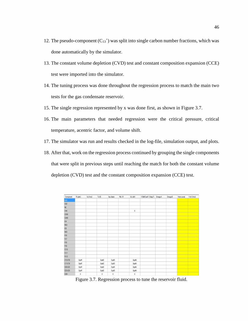
46
12. The pseudo-component (C13
+) was split into single carbon number fractions, which was
done automatically by the simulator.
13. The constant volume depletion (CVD) test and constant composition expansion (CCE)
test were imported into the simulator.
14. The tuning process was done throughout the regression process to match the main two
tests for the gas condensate reservoir.
15. The single regression represented by x was done first, as shown in Figure 3.7.
16. The main parameters that needed regression were the critical pressure, critical
temperature, acentric factor, and volume shift.
17. The simulator was run and results checked in the log-file, simulation output, and plots.
18. After that, work on the regression process continued by grouping the single components
that were split in previous steps until reaching the match for both the constant volume
depletion (CVD) test and the constant composition expansion (CCE) test.
Figure 3.7. Regression process to tune the reservoir fluid.

47
3.3 RESERVOIR GAS CONDENSATE PROPERTIES
This section introduces the correlations used to estimate the gas deviation factor,
gas viscosity, and isothermal compressibility. These gas properties are very important for
the well testing and well deliverability calculations to count the change in gas properties
with respect to pressure. Laboratory measurement is the most precise way to determine gas
properties. However, correlation techniques are an alternative way in the absence of
laboratory measurement data. On the other hand, these methods are used to validate the
results from the laboratory measurements. The following are the brief definitions of the gas
properties that were determined and the correlations methods used for each property.
3.3.1 Gas Deviation Factor. Gas deviation factor is also known as gas
compressibility or Z-factor and is defined as the ratio of actual volume at reservoir
conditions to the ideal volume at surface conditions (Ahmed, 2000).
The gas deviation factor is the term used most in engineering applications such as
estimation gas reserves, design of gas separator, transient pressure analysis in gas wells,
and design pipelines for the transmission of produced gas. Several correlations estimate the
gas deviation factor, and most of these correlations are functions of pseudo-reduced
pressure, (𝑃𝑃𝑝𝑝𝑝𝑝) Equation 3.8, pseudo-reduced temperature, (𝑇𝑇𝑝𝑝𝑝𝑝) Equation 3.9, and gas
gravity (𝛾𝛾𝑔𝑔) (McCain, 1991).
𝑇𝑇𝑝𝑝𝑝𝑝 = 𝑇𝑇𝑅𝑅𝑇𝑇𝑐𝑐
(3.8)
𝑃𝑃𝑝𝑝𝑝𝑝 = 𝑃𝑃𝑅𝑅𝑃𝑃𝑐𝑐
(3.9)
Equations 3.10 and 3.11 are pseudo-critical pressure and the pseudo-critical
temperature for any hydrocarbon mixture.

48
For gas condensate reservoirs the specific gravity for well-stream in Equation 3.12
should be used to estimate the gas deviation factor instead of surface gas gravity. Equation
3.13 is the corrected molecular weight for gas condensate systems (Urayet, 2011).
Where:
𝑇𝑇𝑅𝑅 = Reservoir temperature, (˚R)
𝑃𝑃𝑅𝑅 = Reservoir pressure, (Psi)
𝑇𝑇𝑝𝑝𝑠𝑠 = Pseudo-critical temperature, (˚R)
𝑃𝑃𝑝𝑝𝑠𝑠 = Pseudo-critical pressure, (Psi)
𝑃𝑃𝑝𝑝𝑠𝑠 = ∑ 𝑥𝑥𝑠𝑠𝑠𝑠𝑠𝑠=1 × 𝑃𝑃𝑠𝑠𝑠𝑠 (3.10)
𝑇𝑇𝑝𝑝𝑠𝑠 = ∑ 𝑥𝑥𝑠𝑠𝑠𝑠𝑠𝑠=1 × 𝑇𝑇𝑠𝑠𝑠𝑠 (3.11)
Where:
𝑛𝑛 = number of components, (#)
𝑥𝑥𝑠𝑠 = mole fraction of the component, (mole)
𝑃𝑃𝑠𝑠𝑠𝑠 = Critical pressure of the component, (Psi)
𝑇𝑇𝑠𝑠𝑠𝑠 = Critical temperature of the component, (˚R)
𝛾𝛾𝑔𝑔 =
𝛾𝛾𝑔𝑔𝑠𝑠 + 𝑅𝑅𝑠𝑠𝑠𝑠 × 4,580 𝛾𝛾𝑠𝑠𝑠𝑠1 + 133,000 × 𝑅𝑅𝑠𝑠𝑠𝑠 𝛾𝛾𝑠𝑠𝑠𝑠𝑀𝑀𝑠𝑠
(3.12)
𝑀𝑀𝑠𝑠 = 6,084𝛾𝛾𝐴𝐴𝐴𝐴𝐴𝐴−5.9
(3.13)
If the fluid composition is unknown, the Sutton R.P Equations 3.14 and 3.15 are
used to determine pseudo-critical pressure and temperature.

49
The Wichert and Aziz Equations 3.16 and 3.17 are utilized when impurities are
present in hydrocarbon composition in order to correct the values of pseudo-critical
pressure and temperature.
Where:
𝛾𝛾𝑔𝑔𝑠𝑠 = Specific gravity of the separator gas, (fraction)
𝛾𝛾𝑠𝑠𝑠𝑠 = Specific gravity of the stock tank condensate, (fraction)
𝑅𝑅𝑠𝑠𝑠𝑠 = Gas-oil ratio (Stb condensate/Scf separator gas)
𝑀𝑀𝑠𝑠 = Molecular weight of the tank oil, (Ib/Ib.mole)
𝑃𝑃𝑝𝑝𝑠𝑠 = 756.8 − 131�𝛾𝛾𝑔𝑔� − 3.6�𝛾𝛾𝑔𝑔�2 (3.14)
𝑇𝑇𝑝𝑝𝑠𝑠 = 169.2 − 349.5�𝛾𝛾𝑔𝑔� − 74�𝛾𝛾𝑔𝑔�2 (3.15)
𝑇𝑇𝑝𝑝𝑠𝑠′ = 𝑇𝑇𝑝𝑝𝑠𝑠 − 𝜀𝜀 (3.16)
𝑃𝑃𝑝𝑝𝑠𝑠′ = 𝑃𝑃𝑝𝑝𝑐𝑐 ×𝑇𝑇𝑝𝑝𝑐𝑐′
𝑇𝑇𝑝𝑝𝑐𝑐+𝐵𝐵(1−𝐵𝐵)𝜀𝜀 (3.17)
Where:
𝑇𝑇𝑝𝑝𝑠𝑠′ = Pseudo-critical temperature for gas mixture including the impurities
𝑃𝑃𝑝𝑝𝑠𝑠′ = Pseudo-critical pressure for gas mixture including the impurities
𝜀𝜀 = Defined using Equation 3.18
𝜀𝜀 = 120(𝐴𝐴0.9 − 𝐴𝐴1.6) + 15(𝐵𝐵0.5 − 𝐵𝐵4) (3.18)
𝐴𝐴 = Equation 3.19 is the sum of the mole fraction of hydrogen sulfide and carbone
dioxide

50
According to Dr. Urayet, a professor at the University of Tripoli, the Wichert and
Aziz correlation proves for Libyan gas fields, and the average absolute error for this
correlation around 0.97%. This correlation has accurate results because it works for the gas
mixture that has high concentration of carbon dioxide (CO2).
𝐴𝐴 = 𝑋𝑋(𝐻𝐻2𝑆𝑆) + 𝑋𝑋(𝐶𝐶𝑂𝑂2) (3.19)
𝐵𝐵 = Equation 3.20 is the mole fraction of hydrogen sulfide
𝐵𝐵 = 𝑋𝑋(𝐻𝐻2𝑆𝑆) (3.20)
The following is the main correlation that was used in this study to check and
validate the gas deviation factor from the constant volume depletion (CVD) test.
1. Brill and Beggs’ Method. This method is one of the simplest and most practical
correlations to estimate the gas deviation factor. Brill and Beggs presented this
correlation in 1974 where the Z-factor values are accurate enough for reservoir
engineering applications (Guo et al., 2005). Brill and Beggs’ gas deviation factor
correlation is expressed using Equations 3.21 to 3.27.
𝐴𝐴 = 1.39�𝑇𝑇𝑝𝑝𝑝𝑝 − 0.92�0.5
+ 0.36𝑇𝑇𝑝𝑝𝑝𝑝 − 0.10 (3.21)
𝐵𝐵 = (0.62 − 0.23𝑇𝑇𝑝𝑝)𝑃𝑃𝑝𝑝𝑝𝑝 + �
0.066𝑇𝑇𝑝𝑝 − 0.86
− 0.037� 𝑃𝑃𝑝𝑝𝑝𝑝2 +0.32 𝑃𝑃𝑝𝑝𝑝𝑝6
10𝐸𝐸
(3.22)
𝐶𝐶 = 0.132 − 0.32 log𝑇𝑇𝑝𝑝𝑝𝑝 (3.23)
𝐷𝐷 = 10𝐹𝐹 (3.24)
𝐸𝐸 = 9�𝑇𝑇𝑝𝑝𝑝𝑝 − 1� (3.25)
𝐹𝐹 = 0.3106 − 0.49𝑇𝑇𝑝𝑝𝑝𝑝 + 0.1824𝑇𝑇𝑝𝑝𝑝𝑝2 (3.26)
𝑍𝑍.𝐹𝐹𝑎𝑎𝐹𝐹𝑡𝑡𝐹𝐹𝐹𝐹 = 𝐴𝐴 + 1−𝐴𝐴𝑒𝑒𝐵𝐵
+ 𝐶𝐶𝑃𝑃𝑝𝑝𝑝𝑝𝐷𝐷 (3.27)

51
2. Hall and Yarborough Method. This correlation was introduced by Hall and Yarborough
in 1973 and is a more accurate correlation to estimate the gas deviation factor (Guo et
al., 2005). The correlation is expressed using Equations 3.28 to 3.33
𝑡𝑡 =
1𝑇𝑇𝑝𝑝𝑝𝑝
(3.28)
𝐴𝐴 = 0.06125 𝑡𝑡 𝑒𝑒−1.2(1−𝑡𝑡)2 (3.29)
𝐵𝐵 = 𝑡𝑡(14.76 − 9.76𝑡𝑡 + 4.58𝑡𝑡2) (3.30)
𝐶𝐶 = 𝑡𝑡(90.7 − 242.2𝑡𝑡 + 42.4𝑡𝑡2) (3.31)
𝐷𝐷 = 2.18 + 2.82𝑡𝑡 (3.32)
𝑍𝑍.𝐹𝐹𝑎𝑎𝐹𝐹𝑡𝑡𝐹𝐹𝐹𝐹 = 𝐴𝐴𝑃𝑃𝑝𝑝𝑝𝑝𝑌𝑌
(3.33)
Where Y is the reduced density that solves by using Equation 3.34.
𝑓𝑓(𝑌𝑌) = 𝑌𝑌+𝑌𝑌2+𝑌𝑌3−𝑌𝑌4
(1−𝑌𝑌)3 − 𝐴𝐴𝑃𝑃𝑝𝑝 − 𝐵𝐵𝑌𝑌2 + 𝐶𝐶𝑌𝑌𝐷𝐷 = 0 (3.34)
This non-linear equation solves using numerical techniques, such as the Newton-
Raphson iteration method in Equation 3.35.
𝑓𝑓𝑓𝑓(𝑌𝑌)𝑓𝑓𝑌𝑌
= 1+4𝑌𝑌+4𝑌𝑌2−4𝑌𝑌3+𝑌𝑌4
(1−𝑌𝑌)4 − 2𝐵𝐵𝑌𝑌 + 𝐶𝐶𝐷𝐷𝑌𝑌𝐷𝐷−1 (3.35)
3. Dranchuk & Abou-Kassem’s Method. This correlation was presented in 1975 by
Dranchuk and Abu-Kassem. The authors proposed an eleven constant, as listed in Table
3.2 in order to calculate the gas deviation factor (Guo et al., 2005). The correlation is
summarized in Equation 3.36.
𝑍𝑍 − 𝐹𝐹𝑎𝑎𝐹𝐹𝑡𝑡𝐹𝐹𝐹𝐹 = 1 + �𝐴𝐴1 + 𝐴𝐴2𝑇𝑇𝑝𝑝
+ 𝐴𝐴3𝑇𝑇𝑝𝑝3
+ 𝐴𝐴4𝑇𝑇𝑝𝑝4
+ 𝐴𝐴5𝑇𝑇𝑝𝑝5� 𝜌𝜌𝑝𝑝 + �𝐴𝐴6 + 𝐴𝐴7
𝑇𝑇𝑝𝑝+ 𝐴𝐴8
𝑇𝑇𝑝𝑝2� 𝜌𝜌𝑝𝑝2 − 𝐴𝐴9 �
𝐴𝐴7𝑇𝑇𝑝𝑝
+
𝐴𝐴8𝑇𝑇𝑝𝑝2� 𝜌𝜌𝑝𝑝7 × 𝐴𝐴10[1 + 𝐴𝐴11𝜌𝜌𝑝𝑝2] 𝜌𝜌𝑝𝑝
2
𝑇𝑇𝑝𝑝3 𝑒𝑒−𝐴𝐴11𝜌𝜌𝑝𝑝2 (3.36)
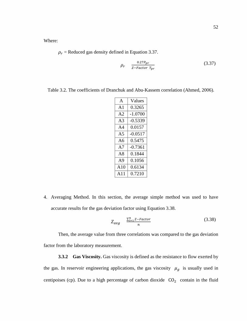
52
Where:
𝜌𝜌𝑝𝑝 = Reduced gas density defined in Equation 3.37.
𝜌𝜌𝑝𝑝 = 0.27𝑃𝑃𝑝𝑝𝑝𝑝𝑍𝑍−𝐹𝐹𝑚𝑚𝑠𝑠𝑡𝑡𝑠𝑠𝑝𝑝 𝑇𝑇𝑝𝑝𝑝𝑝
(3.37)
Table 3.2. The coefficients of Dranchuk and Abu-Kassem correlation (Ahmed, 2006).
A Values A1 0.3265 A2 -1.0700 A3 -0.5339 A4 0.0157 A5 -0.0517 A6 0.5475 A7 -0.7361 A8 0.1844 A9 0.1056 A10 0.6134 A11 0.7210
4. Averaging Method. In this section, the average simple method was used to have
accurate results for the gas deviation factor using Equation 3.38.
𝑍𝑍𝑚𝑚𝑎𝑎𝑔𝑔 = ∑ 𝑍𝑍−𝐹𝐹𝑚𝑚𝑠𝑠𝑡𝑡𝑠𝑠𝑝𝑝𝑀𝑀𝑀𝑀=1
𝑠𝑠 (3.38)
Then, the average value from three correlations was compared to the gas deviation
factor from the laboratory measurement.
3.3.2 Gas Viscosity. Gas viscosity is defined as the resistance to flow exerted by
the gas. In reservoir engineering applications, the gas viscosity (𝜇𝜇𝑔𝑔) is usually used in
centipoises (cp). Due to a high percentage of carbon dioxide (CO2) contain in the fluid

53
composition, Lee, Gonzalez, and Eakin numerical correlation was used in order to obtain
accurate results.
1. Lee, Gonzalez, and Eakin Correlation. This correlation was introduced in 1966 by Lee,
Gonzalez, and Eakin. Many viscosity correlations in petroleum industry have been
derived from this correlation. It is one of the most accurate correlations for the
calculation of the gas viscosity (Ugwu et al., 2016). The correlation theoretical concept
can be expressed in Equation 3.39 to 3.43.
𝜇𝜇𝑔𝑔 = 10−4 𝐾𝐾 𝑒𝑒𝑥𝑥𝑒𝑒(𝑋𝑋 𝜌𝜌𝑌𝑌) (3.39)
Where:
𝜌𝜌 = 1.4935 (10−3) 𝑃𝑃𝑅𝑅 𝑀𝑀𝑤𝑤𝑍𝑍 𝑇𝑇𝑅𝑅
(3.40)
𝐾𝐾 =
(9.379 + 0.01607 𝑀𝑀𝑀𝑀)𝑇𝑇𝑅𝑅1.5
(209.2 + 19.26 𝑀𝑀𝑀𝑀 + 𝑇𝑇𝑅𝑅) (3.41)
𝑋𝑋 = 3.448 +
986.4𝑇𝑇𝑅𝑅
+ 0.01009 𝑀𝑀𝑀𝑀 (3.42)
𝑌𝑌 = 2.447 − 0.2224𝑋𝑋 (3.43)
𝜌𝜌 = Gas density, (Ib/ft3)
𝑃𝑃𝑅𝑅 = Reservoir pressure, (Psi)
𝑇𝑇𝑅𝑅 = Reservoir temperature, (0R)
𝑀𝑀𝑀𝑀 = Molecular weight of the gas mixture, (Ib/gmole)
3.3.3 Isothermal Compressibility. The isothermal compressibility of the gas is
defined in Equation 3.44.
𝐶𝐶 = − 1𝑉𝑉
𝑓𝑓𝑉𝑉𝑓𝑓𝑃𝑃
(3.44)

54
Equations 3.45 to 3.47 are the mathematical derivation of the isothermal
compressibility (Guo et al., 2005).
𝐶𝐶𝐶𝐶 = − 1𝑉𝑉
𝑓𝑓𝑉𝑉𝑓𝑓𝑃𝑃
= − 𝑃𝑃𝑅𝑅𝑍𝑍 𝑠𝑠 𝑅𝑅 𝑇𝑇𝑅𝑅
𝑓𝑓𝑓𝑓𝑃𝑃
�𝑍𝑍 𝑠𝑠 𝑅𝑅 𝑇𝑇𝑅𝑅𝑃𝑃𝑅𝑅
� (3.45)
𝐶𝐶𝐶𝐶 = −𝑃𝑃𝑍𝑍�𝑍𝑍 �−1
𝑃𝑃𝑅𝑅2�+ 1
𝑃𝑃𝑅𝑅 𝑓𝑓𝑍𝑍𝑓𝑓𝑃𝑃� (3.46)
𝐶𝐶𝐶𝐶 = 1𝑃𝑃𝑅𝑅− 1
𝑍𝑍 𝑓𝑓𝑍𝑍𝑓𝑓𝑃𝑃
(3.47)
3.4 GAS WELL TESTING INTERPRETATION
Well testing interpretation in gas wells is more complex than the analysis in oil
wells due to the gas properties that are affected by changing pressures. As a result, the
equation of pressure transmission through gases in a reservoir porous medium is the
nonlinear equation. All of the solutions derived for well-testing interpretation were
designed based on slightly compressible filled in reservoirs. However, these solutions are
applicable to use in the gas well-testing interpretation by substituting the pressure and time
with pseudo-pressure and pseudo-time, as shown in Equation 3.48 (Spivey et al., 2013).
𝜕𝜕𝑚𝑚(𝑃𝑃)𝜕𝜕𝑝𝑝2
+ 1𝑝𝑝
𝜕𝜕𝑚𝑚(𝑃𝑃)𝜕𝜕𝑝𝑝
= ∅ 𝜇𝜇 𝐶𝐶𝑡𝑡𝑘𝑘
𝜕𝜕𝑚𝑚(𝑃𝑃)𝜕𝜕𝑡𝑡
(3.48)
Equation 3.48 is a linear equation after substituting the pressure by 𝑚𝑚(𝑒𝑒), but the
term ∅ 𝜇𝜇 𝐶𝐶𝑡𝑡𝑘𝑘
is still a function of pressure. In practice, this remaining nonlinearity is not
usually of consequence. It is often permissible to treat the equation as linear, substituting
the values of viscosity (μ) and compressibility (Ct) defined at the initial reservoir pressure
(Pi) (or at the highest pressure measured during the test if the initial reservoir pressure is
not known) (Spivey et al., 2013).

55
This section focuses on the interpretation of the data for both drawdown and
buildup tests from the flow-after-flow test by performing different plot approaches as
follows: pressure derivative (log-log) plot as a diagnostic plot to detect the flow regimes,
superposition plot (semi-log plot) in order to obtain the reservoir characteristics, type curve
analysis for more confident interpretation, and the use of commercial well-testing software
(Saphir) to confirm outcomes and obtain deep interpretation results.
3.4.1 Pressure Derivative Plot. The pressure derivative (log-log plot) is a
modern method for well-testing interpretation. This technique is a key factor used as a
diagnostic to evaluate different parameters such as reservoir permeability, wellbore
storage, reservoir boundary, reservoir behavior, and flow regimes. The concept of pressure
derivative in transient pressure analysis was first found by Tiab and Kumar in 1980. Since
that time, several publications have been presented on the application of using pressure
derivative. Bourdet (1989) illustrated how to simplify the analysis to make the well-testing
interpretation more precise and easy. Nowadays, the Bourdet pressure derivative is used in
all commercial well-testing software analysis, including Kappa Saphir.
Before the pressure derivate is discussed, the main input parameters are introduced
in the following sections.
3.4.1.1 Single-phase pseudo-pressure. Single-phase pseudo-pressure is essential
in transient pressure analysis gas reservoirs because of change in the gas properties with
pressure. As a result, this method is used to account for the variable compressibility and
viscosity of gas with respect to pressure. This technique was introduced by Al-Hussainy
and Ramey in 1966. The pseudo-gas potential pressure is defined in Equation 3.49. This
method is used only when a single phase is present in the reservoir. Therefore, if condensate

56
is present, it is assumed that its saturation is below the critical gas saturation, meaning the
condensate is immobile. The impact of the condensate on the relative permeability curve
is negligible (Raghavan et al., 1995).
𝑚𝑚(𝑒𝑒) = 2∫ 𝑝𝑝𝜇𝜇𝐿𝐿 𝑧𝑧𝐿𝐿
𝑝𝑝𝑝𝑝𝑟𝑟𝑓𝑓𝑝𝑝0
𝑑𝑑𝑒𝑒 (3.49)
Where:
𝑚𝑚(𝑒𝑒) = Pseudo-gas potential pressure, (Psi2/cp)
𝑍𝑍 = Gas deviation factor, (Unit-less)
𝜇𝜇 = Gas viscosity, (cp)
𝑒𝑒0 = Based pressure that usually is the lowest pressure (surface pressure condition)
of the range of pressures during the test, (Psi)
𝑒𝑒𝑝𝑝𝑒𝑒𝑓𝑓 = Reference pressure that usually is the initial pressure (𝑒𝑒𝑠𝑠), (Psi)
The PVT-fluid properties were determined and validated in the section of the
reservoir gas condensate properties, where the trapezoidal method has been used by these
properties in Equation 3.50 to obtain pseudo-gas potential pressure.
𝑚𝑚(𝑒𝑒) = 2∑ 12
𝑠𝑠𝑠𝑠=2 �� 𝑝𝑝
𝜇𝜇 𝑧𝑧�𝑠𝑠−1
+ � 𝑝𝑝𝜇𝜇 𝑧𝑧�𝑠𝑠� (𝑒𝑒𝑠𝑠 − 𝑒𝑒𝑠𝑠−1) (3.50)
3.4.1.2 Adjusted pressure. Unfortunately, the real gas pseudo-pressure unit is a
function of Psi2/cp, which is the magnitude on the order of 109 Psi2/cp for a pressure of
5,000 psi (Spivey et al., 2013). For convenes unit, the adjusted pressure in Equation 3.51
is normalized from the real gas pseudo-pressure (Meunier et al., 1987).
(𝑒𝑒𝑚𝑚) = 𝜇𝜇�𝑝𝑝𝑝𝑝𝑟𝑟𝑓𝑓�×𝑍𝑍�𝑝𝑝𝑝𝑝𝑟𝑟𝑓𝑓�2 𝑝𝑝𝑝𝑝𝑟𝑟𝑓𝑓
𝑚𝑚(𝑒𝑒) (3.51)
Where:
𝑒𝑒𝑚𝑚 = Adjusted pressure, (Psi)

57
3.4.1.3 Pseudo-time and adjusted time. Agarwal introduced pseudo-time in 1979,
and later Lee and Holditch described pseudo-time use in 1982. Agarwal’s pseudo-time is
defined in Equation 3.52.
𝑡𝑡𝑝𝑝𝑠𝑠𝑒𝑒𝑓𝑓𝑓𝑓𝑠𝑠 = ∫ 1𝜇𝜇 𝐶𝐶𝑡𝑡
𝑑𝑑𝑡𝑡𝑡𝑡0 (3.52)
The Agarwal definition of pseudotime does not have a unit of time, which makes
the data plots more difficult for visual examination. As a result, Meunier et al. (1987)
normalized the Agarwal equation to have the time unit, called the adjusted time, as defined
in Equation 3.53.
𝑡𝑡𝑚𝑚 = 𝜇𝜇𝑠𝑠 𝐶𝐶𝑡𝑡𝑠𝑠 ∫1
𝜇𝜇 𝐶𝐶𝑡𝑡𝑑𝑑𝑡𝑡𝑡𝑡
0 (3.53)
Where:
𝑡𝑡𝑚𝑚 = Adjusted time, (hrs)
𝑡𝑡𝑝𝑝𝑠𝑠𝑒𝑒𝑓𝑓𝑓𝑓𝑠𝑠 = Pseudo-time, (unitless)
𝜇𝜇𝑠𝑠 = Gas viscosity at the reference pressure, (cp)
𝐶𝐶𝑡𝑡𝑠𝑠 = Gas compressibility at the reference pressure, (Psi-1)
3.4.1.4 Superposition in time. The principle of superposition is a powerful concept
used to solve complex cases in both pressure transient analysis (PTA) and rate transient
analysis (RTA). In this thesis, the superposition approach is utilized for the multi-rate
production case, which is used to convert the multi-rate production to an equivalent single
rate model. Figure 3.10 shows the pressure drop response at the time n that can be defined
in Equation 3.54.
ΔP = pressure drop from the well due to qi throughout the entire flow period (flow time=tn)
+ pressure drop from the well producing at (qi+1-qi), commencing at the time ti (flow

58
time=tn-ti) + pressure drop from the well producing at (qn-qi+1), commencing at the time
ti+1 (flow time = tn-ti+1). Therefore, as shown in Figure 3.8, the total pressure drop is defined
as follows:
∆𝑃𝑃 = ∆𝑃𝑃𝑠𝑠 + ∆𝑃𝑃𝑠𝑠+1 + ∆𝑃𝑃𝑠𝑠 (3.54)
Superposition in time for the buildup test and multi-rate test is defined in Equation
3.55.
𝑆𝑆𝑆𝑆𝑒𝑒(∆𝑡𝑡𝑠𝑠) = ∑ � 𝑞𝑞𝑀𝑀−𝑞𝑞𝑀𝑀−1𝑞𝑞𝑀𝑀−𝑞𝑞𝑀𝑀−1
× log[𝑡𝑡𝑠𝑠 − 𝑡𝑡𝑠𝑠 + ∆𝑡𝑡𝑠𝑠] + log∆𝑡𝑡𝑠𝑠�𝑠𝑠−1𝑠𝑠=1 (3.55)
Where:
𝑆𝑆𝑆𝑆𝑒𝑒(∆𝑡𝑡𝑠𝑠) = superposition time at certain time during the test, (hrs)
𝑞𝑞𝑠𝑠 = flow rate at certain period, (MMscf/day)
𝑞𝑞𝑠𝑠 = last flow rate before the buildup test, (MMscf/day)
𝑡𝑡𝑠𝑠 = the time during the period of first flow rate, (hrs)
𝑡𝑡𝑠𝑠 = the final time until the buildup test starts, (hrs)
Figure 3.8. Multi-rate flow profile and pressure response due to different rates (modified
from Liang et al., 2013).
3.4.1.5 The Bourdet derivative. In this thesis, the Bourdet pressure derivative
technique is used in both drawdown and buildup analysis. This technique computes the

59
derivative from the slope points in the semi-log plot where the x-axis is the natural log of
time and the y-axis is the pressure, as shown in Figure 3.9.
Figure 3.9. Bourdet derivative, semi-log and log-log (Dynamic Flow Analysis, Kappa,
2012).
Equations 3.56 and 3.58 are simple and standard techniques to determine the
pressure derivative for the buildup and drawdown analysis.
For a drawdown:
𝛥𝛥𝑒𝑒′ = 𝑓𝑓∆𝑝𝑝𝑓𝑓 ln(∆𝑡𝑡)
= ∆𝑡𝑡 𝑓𝑓∆𝑝𝑝𝑓𝑓∆𝑡𝑡
(3.56)
Where:
∆𝑒𝑒 = 𝑒𝑒𝑠𝑠 − 𝑒𝑒𝑤𝑤𝑓𝑓(∆𝑡𝑡) (3.57)
For buildup and multi-rate:
𝛥𝛥𝑒𝑒′ = 𝑓𝑓∆𝑝𝑝𝑓𝑓 sup(∆𝑡𝑡)
(3.58)
∆𝑒𝑒 = 𝑒𝑒𝑤𝑤𝑠𝑠(∆𝑡𝑡) − 𝑒𝑒𝑤𝑤𝑓𝑓(𝑡𝑡𝑒𝑒) (3.59)
Where:
Equations 3.57 and 3.59 are the pressure drop for the buildup and drawdown analysis,
respectively.

60
Where:
𝛥𝛥𝑒𝑒′ = Pressure derivative, (unitless)
𝛥𝛥𝑒𝑒 = Pressure drop, (Psi)
𝛥𝛥𝑡𝑡 = Time, (hrs)
𝑡𝑡𝑒𝑒 = Production time, (hrs)
𝑒𝑒𝑤𝑤𝑓𝑓 = Bottomhole flowing pressure, (Psi)
𝑒𝑒𝑤𝑤𝑠𝑠 = Shut-in pressure, (Psi)
𝑠𝑠𝑆𝑆𝑒𝑒(𝛥𝛥𝑡𝑡) = Superposition time, (hrs)
Figure 3.10. Schematic of Bourdet derivative algorithm (Dynamic Flow Analysis, Kappa,
2012).
∆𝑒𝑒′ =
�∆𝑝𝑝1∆𝑀𝑀1∆𝑥𝑥2+
∆𝑝𝑝2∆𝑀𝑀2
∆𝑡𝑡𝑥𝑥1�
∆𝑥𝑥1+∆𝑥𝑥2
(3.60)
Equation 3.60 was used for the interpretation in this thesis because the real data
needs more smoothing due to the noisy pressure data during the test operation. Figure 3.10

61
illustrates the Bourdet derivative algorithm that is widely used by commercial software for
the well-testing interpretations.
3.4.2 Type Curve Analysis. Type curve is a powerful technique used for both
drawdown and buildup analysis. The type curve shows the dimensionless pressure function
versus the dimensionless time function that are the solutions of the flow equation
(diffusivity equation). The following are the most common used log-log type curve:
Agarwal, Al-Hussainy, and Ramey (1970), Earlougher and Kersch (1974), Gringarten,
Ramey, and Rhagavan (1974), and finally, Gringarten and Bourdet (1979).
In this thesis, the Gringarten and Bourdet type curve, as shown in Figure 3.11, was
utilized for the analysis in order to determine the reservoir permeability, skin, and wellbore
storage.
Figure 3.11. Gringarten and Bourdet type curve (Gringarten et al., 1979).
3.4.3 Interpretation procedures. The flow-after-flow tests were conducted in
the North African field in 2009 and 2014. This type of test consists of four drawdown tests
62
and one buildup test. This section basically focuses on the analysis of the test in 2009.
Consecutively, the same procedure can be used for the test in 2014. The following steps
are the preparing the data for the analysis, and then the buildup test was analyzed using
pressure derivative and superposition plot and type curve analysis.
1. The transient pressure data were gathered and filtrated for certain periods of time steps
to avoid repeating the same value of pressure.
2. In filtration process for the pressure range, the time interval should be consistent with
each step. For example, the first time interval was 60 sec, followed by a 90 sec time
period, etc.
3. An Excel spreadsheet was created, and the pressure, time, and flow rates were entered
as input-data for the analysis.
4. The gas flow rate for each drawdown was corrected by counting the condensate flow
rate to determine the equivalent flow rate in Equation 3.61.
𝑞𝑞𝑔𝑔𝑠𝑠 = 𝑞𝑞𝑔𝑔𝑠𝑠 + 𝑞𝑞𝑠𝑠 × 3,003 × (1.03 − 𝛾𝛾𝑠𝑠) + 𝑞𝑞𝑤𝑤 × 7,390 (3.61)
Where:
𝑞𝑞𝑔𝑔𝑠𝑠 = Equivalent gas flow rate, (MMscf/day)
𝑞𝑞𝑔𝑔𝑠𝑠 = Gas flow rate, (MMscf/day)
𝑞𝑞𝑠𝑠 =Condensate flow rate, (Rbbl/day)
𝑞𝑞𝑤𝑤 = Water flow rate, (Rbbl/day)
𝛾𝛾𝑠𝑠 = Condensate specific gravity, (unitless)

63
5. Before the analysis began, the equivalent flow rates were checked using derivative
overlay, as shown in Figure 3.12. This technique was used in order to have one mutual
infinite acting radial flow (IARF) for four drawdowns.
Figure 3.12. Derivative overlay for four drawdowns before adjusted flow rates.
6. If not, the equivalent flow rates were adjusted until four drawdown pressure derivatives
overlaid each other, as shown in Figure 3.13.
Figure 3.13. Derivative overlay for four drawdowns after adjusted flow rates.

64
7. After the overlay process, the pressure derivative and superposition plot method was
used, followed by Gringarten type curve method for more confident and accurate results.
3.4.4 Pressure Derivative and Superposition Plot.
1. Superposition in time, pressure derivative, and pressure drop were determine in order to
perform the pressure derivative for buildup test, as shown in Figure 3.14.
Figure 3.14. Pressure derivative plot for buildup test.
2. The radial flow regions were detected on the plot, as shown in Figure 3.15. These
regions are important to determine the reservoir permeability.
Figure 3.15. Radial flow regions on the pressure derivative plot.

65
3. Then, a superposition plot was created by plotting the pseudo-gas pressure and
superposition in time on the semi-log plot in order to determine the slope of each radial
flow region. After that, permeability and skin factor at each region were calculated using
Equations 3.62 and 3.63.
𝐾𝐾 = 162.6 𝑞𝑞𝐿𝐿𝑐𝑐 𝛽𝛽𝐿𝐿 𝜇𝜇𝐿𝐿|𝑚𝑚|ℎ
(3.62)
Where:
𝑚𝑚 = Slope, (psi2/cp/cycle)
𝐾𝐾 = Reservoir permeability, (md)
𝑞𝑞𝑔𝑔𝑠𝑠 = Equivalent gas flow rate, (MMscf/day)
𝛽𝛽𝑔𝑔 = Gas formation volume factor, (ft3/scf)
𝜇𝜇𝑔𝑔 = Gas viscosity, (cp)
ℎ = Net pay thickness, (ft)
𝑆𝑆 = 1.151 �𝑚𝑚(𝑝𝑝𝑤𝑤𝑓𝑓𝐿𝐿)−𝑚𝑚(𝑝𝑝1ℎ𝑝𝑝)|𝑚𝑚| − log � 𝑘𝑘
𝜑𝜑𝜇𝜇𝑠𝑠𝑡𝑡𝑝𝑝𝑤𝑤2�+ 3.23� (3.63)
Where:
𝑆𝑆 = Skin factor, (unitless)
𝑚𝑚(𝑒𝑒𝑤𝑤𝑓𝑓𝑠𝑠) = Pseudo-gas pressure at zero time, (psi2/cp)
𝑚𝑚(𝑒𝑒1ℎ𝑝𝑝) = Pseudo-gas pressure at one hour, (psi2/cp)
∅ = Porosity, (fraction)
𝐶𝐶𝑡𝑡 = Total compressibility, (psi-1)
𝐹𝐹𝑤𝑤 = Wellbore radius, (ft)

66
3.4.4.1 Gringarten type curve.
1. The adjusted pressure and superposition in time were plotted on the log-log scale, then
overlaid on the Gringarten type curve.
2. The scale for both the pressure derivative and Gringarten type curve should be
consistent, which means both plots should have the same cycle numbers in the x-axis
and y-axis.
3. The derivative plot was moved over the Gringarten type curve until the match of the
radial flow region was reached, as shown in Figure 3.16.
4. Then, the main points were picked on the plot where certain superposition in time and
pressure drop overlay dimensionless time (𝑡𝑡𝐷𝐷 ) and dimensionless pressure(𝑒𝑒𝐷𝐷 ), as
indicated in Figure 3.16 by the red arrows, and listed in Table 3.3.
Figure 3.16. Gringarten type curve for the first radial flow region.
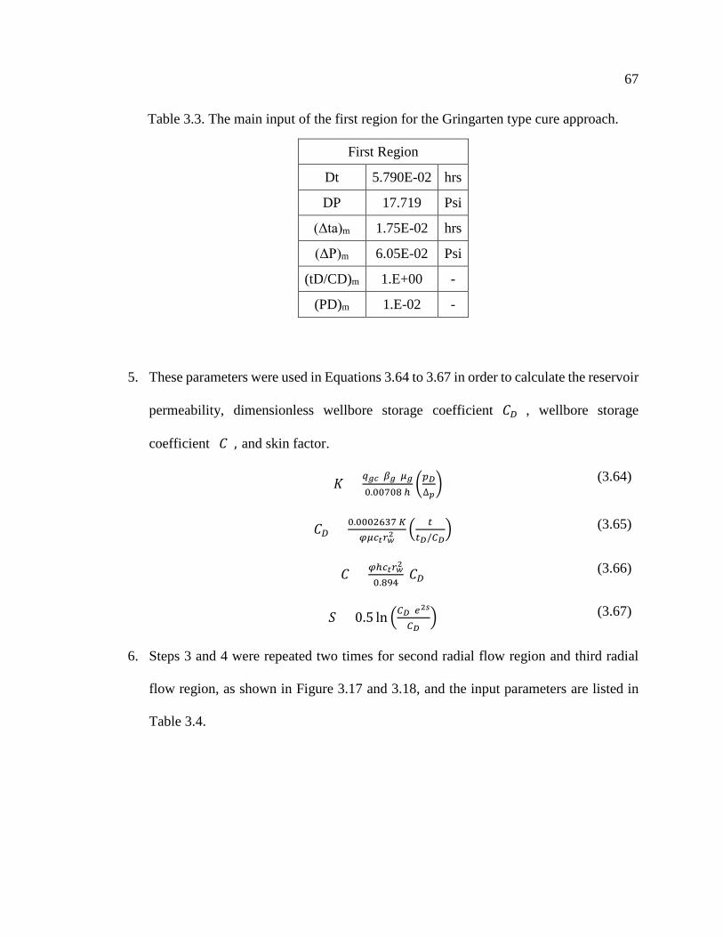
67
Table 3.3. The main input of the first region for the Gringarten type cure approach.
First Region
Dt 5.790E-02 hrs
DP 17.719 Psi
(Δta)m 1.75E-02 hrs
(ΔP)m 6.05E-02 Psi
(tD/CD)m 1.E+00 -
(PD)m 1.E-02 -
5. These parameters were used in Equations 3.64 to 3.67 in order to calculate the reservoir
permeability, dimensionless wellbore storage coefficient (𝐶𝐶𝐷𝐷 ), wellbore storage
coefficient (𝐶𝐶), and skin factor.
𝐾𝐾 = 𝑞𝑞𝐿𝐿𝑐𝑐 𝛽𝛽𝐿𝐿 𝜇𝜇𝐿𝐿0.00708 ℎ
�𝑝𝑝𝐷𝐷∆𝑝𝑝� (3.64)
𝐶𝐶𝐷𝐷 = 0.0002637 𝐾𝐾𝜑𝜑𝜇𝜇𝑠𝑠𝑡𝑡𝑝𝑝𝑤𝑤2
� 𝑡𝑡𝑡𝑡𝐷𝐷/𝐶𝐶𝐷𝐷
� (3.65)
𝐶𝐶 = 𝜑𝜑ℎ𝑠𝑠𝑡𝑡𝑝𝑝𝑤𝑤2
0.894 𝐶𝐶𝐷𝐷 (3.66)
𝑆𝑆 = 0.5 ln �𝐶𝐶𝐷𝐷 𝑒𝑒2𝑠𝑠
𝐶𝐶𝐷𝐷� (3.67)
6. Steps 3 and 4 were repeated two times for second radial flow region and third radial
flow region, as shown in Figure 3.17 and 3.18, and the input parameters are listed in
Table 3.4.

68
Figure 3.17. Gringarten type curve for the second radial flow region.
Figure 3.18. Gringarten type curve for the third radial flow region.

69
Table 3.4. The main input of the second and third regions for the Gringarten type cure
approach.
Parameter Second Region Third Region Unit
Dt 5.790E-02 5.790E-02 hrs
DP 17.719 17.719 Psi
(Δta)m 1.05E-02 8.20E-03 hrs
(ΔP)m 4.38E-02 2.95E-02 Psi
(tD/CD)m 1.E+00 1.E+00 -
(PD)m 1.E-02 1.E-02 -
3.4.4.2 Kappa Saphir software. Kappa engineering package consists of several
software related to reservoir and production engineering applications. In this thesis, Saphir
software was utilized for the analysis of transient pressure data because it is widely used
by most companies in petroleum industry. The following are step-by-step procedures that
introduce how to interpret the well-testing data using Saphir software.
1. The reservoir data were entered in the analysis information window, as shown in Figure
3.19.
Figure 3.19. The main reservoir parameters.

70
2. PVT data were imported into the software where the PVT-P file was used to define the
reservoir fluid properties, as shown in Figure 3.20.
Figure 3.20. PVT data.
3. The pressures, time, and flow rates were imported into the software. Then, the data was
synchronized in the edit rate and pressure (QAQC) section in order to have accurate
interpretation.
4. The flow-after-flow data were divided into drawdowns data and buildup data, where the
analysis was started with drawdown analysis in order to obtain the skin factor for each
drawdown period.
5. Skin factors were used to determine the non-Darcy flow coefficient.
6. The pressure derivative was extracted for the first drawdown, and then the analytical
model was used to match the model line represented in red with the actual data.
7. Because the early data did not fall on the unit slope, and this behavior is defined by
changing wellbore storage, Hegeman model was used to have precise results.

71
8. Figure 3.21 shows the first drawdown pressure derivative where the software model
matched the actual data perfectly.
Figure 3.21. The interpretation for the first drawdown.
9. Steps 5 and 6 were repeated for the second, third, and fourth drawdown in order to have
a perfect match, as shown in Figure 3.22, 3.23, and 3.24.
Figure 3.22. The interpretation for the second drawdown.
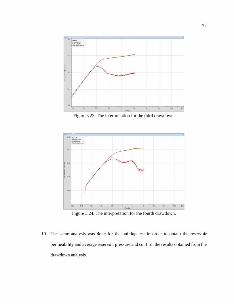
72
Figure 3.23. The interpretation for the third drawdown.
Figure 3.24. The interpretation for the fourth drawdown.
10. The same analysis was done for the buildup test in order to obtain the reservoir
permeability and average reservoir pressure and confirm the results obtained from the
drawdown analysis.

73
11. Figure 3.25 illustrates the analysis of the buildup test where the second and third radial
flow regions were matched perfectly.
12. In order to determine the non-Darcy coefficient flow that is an important parameter
with skin and permeability to match the pressure test with the model, there are two
methods: rate-dependent skin or time-dependent skin.
Figure 3.25. The interpretation for the buildup.
13. The rate-dependent skin was first used where the four drawdown overlaid together, as
shown in Figure 3.26, and the mutual radial flow region was selected in order to
perform the skin versus gas flow rate plot.
14. Figure 3.27 shows the skin versus gas flow rate where the non-Darcy coefficient flow
was obtained.
15. The history pressure improvement was run to match the model with the flow-after-
flow test, as shown in Figure 3.28.

74
Figure 3.26. Derivative overlay for the four drawdowns.
Figure 3.27. Rate-dependent skin plot.
Figure 3.28. The history pressure before reaching the match using rate-dependent skin.

75
16. In order to improve the match, the average reservoir pressure and skin factor at the
zero flow rate and non-Darcy flow coefficient were modified until the match was
reached, as shown in Figure 3.29.
Figure 3.29. The history pressure after reaching the match using rate-dependent skin.
3.5 WELL DELIVERABILITY
The well deliverability calculations were used in this research based on the back-
pressure equations where three equations were utilized to determine the absolute open flow
(AOF) potential and performed the inflow performance relationship (IPR). This research
studied two flow-after-flow tests in 2009 and 2014, where this section focuses on the
interpretation of the test in 2009. The same analysis was used for the test in 2014. The
following step-by-step procedures to determine the deliverability for the well A7 using
Excel, Kappa Saphir software, and Prosper software.

76
3.5.1 Excel Sheet Calculation.
1. The bottomhole flowing pressure points for each drawdown test were picked from the
stabilization period at the end of each drawdown test, as shown in Figure 3.30 by the
red circle.
2. Table 3.5 lists the bottomhole flowing pressure versus equivalent gas flow rate in each
drawdown.
Figure 3.30. Flow-after-flow test.
Table 3.5. Main input data for the deliverability calculations.
Test Flowing Pressure Equivalent Gas Flow Rate
# Psi MM Scf/day
0 3,359.10 0
1 3,338.00 27.57
2 3,333.55 32.40
3 3,328.15 37.79
4 3,322.86 42.80

77
3. The pressure at test number zero is the average reservoir pressure that has been
determined from well-testing interpretation using Saphir software.
4. The first method of backpressure equations is the empirical method that was used as
described in the following.
a. Calculate the pressure difference squared between the flowing pressure at each test
and the average reservoir pressure, as listed in Table 3.6.
Table 3.6. Input calculation data in the empirical method.
Test Pavg2-Pwf
2 Test Pavg2-Pwf
2 Test Pavg2-Pwf
2
# Psi2 # Psi2 # Psi2
0 0.00E+00 2 1.71E+05 4 2.42E+05
1 1.41E+05 3 2.07E+05 - -
b. Plot the data points on the log-log scale, where the x-axis represents the equivalent
gas flow rate and the y-axis represents the pressure difference squared, as shown in
Figure 3.31.
c. The 𝑛𝑛 and 𝐶𝐶 values were determined from the extrapolated line equation or by using
the empirical Equation 3.68.
𝑞𝑞𝑔𝑔 = 𝐶𝐶 × �𝑃𝑃𝑚𝑚𝑎𝑎𝑔𝑔2 − 𝑃𝑃𝑤𝑤𝑓𝑓2 �𝑠𝑠
(3.68)
d. Absolute open potential flow was obtained using the empirical method plot, as
shown in Figure 3.32, or using Equation 3.69 by assuming the flowing bottomhole
pressure is 14.7 psi.

78
Where:
𝑞𝑞𝑔𝑔 = Equivalent gas flow rate, (MMscf/day)
𝑃𝑃𝑤𝑤𝑓𝑓 = Bottomhole flowing pressure, (psi)
𝑃𝑃𝑚𝑚𝑎𝑎𝑔𝑔 = Average reservoir pressure, (psi)
𝑛𝑛 = Performance exponent constant, (unitless)
𝐶𝐶 = Inflow (or performance) coefficient, (MMscf/day/psi2)
Figure 3.31. Deliverability calculation (empirical method).
Figure 3.32. Deliverability calculation (empirical method).

79
e. The equation was used to determine the gas flow rates at wide range of pressures
in order to contrast the inflow performance relationship plot (IPR).
𝑞𝑞𝑔𝑔 = 𝐶𝐶 × �𝑃𝑃𝑚𝑚𝑎𝑎𝑔𝑔2 − 14.72�𝑠𝑠
(3.69)
5. The second method of backpressure equations is the theoretical (modified) method that
was used as described in the following steps.
a. The pressure difference squared was calculated between the flowing pressure at
each test and the average reservoir pressure and then divided by the equivalent gas
flow rate at each test, as listed in Table 3.7.
Table 3.7. Input calculation data in the theoretical method.
Test Pavg2-Pwf
2/Qg
# Psi2/ MM Scf/day
0 0.00E+00
1 5.13E+03
2 5.28E+03
3 5.48E+03
4 5.66E+03
b. The data points on the Cartesian scale were plotted, where the x-axis represents the
equivalent gas flow rate and y-axis represents the pressure difference squared
divided by the equivalent gas rate at each test, as shown in Figure 3.33.
c. The 𝑎𝑎 and 𝑏𝑏 values were obtained from the extrapolated line equation or by using
Equation 3.70 or Equation 3.71.

80
d. Solver function in Excel was used in order to obtain the value of absolute open flow
(AOF) potential.
𝑃𝑃𝑚𝑚𝑎𝑎𝑔𝑔2 − 𝑃𝑃𝑤𝑤𝑓𝑓2 = 𝑎𝑎. 𝑞𝑞𝑔𝑔 + 𝑏𝑏. 𝑞𝑞𝑔𝑔2 (3.70)
𝑃𝑃𝑀𝑀𝑎𝑎𝐿𝐿2 −𝑃𝑃𝑤𝑤𝑓𝑓2
𝑞𝑞𝐿𝐿= 𝑎𝑎. +𝑏𝑏. 𝑞𝑞𝑔𝑔 (3.71)
Figure 3.33. Deliverability calculation (theoretical method).
6. The final method of backpressure equations is the exact (pseudo-gas potential) method
that depends on the pseudo-gas potential pressures in its calculation instead of using the
normal pressures. The following are the steps that were utilized in the exact method
calculations.
a. The normal pressure at each test number was converted to pseudo-gas potential
pressure using the equation that resulted from the single-phase calculation
(Equation 3.50).
b. The pseudo-gas potential pressure difference was calculated between the flowing
pseudo-gas potential pressure at each test and the average pseudo-gas potential

81
reservoir pressure and then divided by the equivalent gas flow rate at each test, as
listed in Table 3.8.
Table 3.8. Input calculation data in the exact method.
Test [m(Pavg)-m(Pwf)]/Qg Test [m(Pavg)-m(Pwf)]/Qg
# Psi2/CP # Psi2/CP
0 0.00E+00 4 2.67E+05
1 2.41E+05 - -
2 2.49E+05 - -
3 2.58E+05 - -
c. The data points on the Cartesian scale were plotted where the x-axis represents the
equivalent gas flow rate and y-axis represents the difference between the flowing
pseudo-gas potential pressure at each test and the average pseudo-gas potential
reservoir pressure divided by the equivalent gas flow rate at each test, as shown in
Figure 3.34.
Figure 3.34. Deliverability calculation (Exact method).

82
d. The 𝐴𝐴 and 𝐵𝐵 values were determined from the extrapolated line equation or using
Equation 3.72 or Equation 3.73.
𝑚𝑚�𝑃𝑃𝑚𝑚𝑎𝑎𝑔𝑔� − 𝑚𝑚�𝑃𝑃𝑤𝑤𝑓𝑓� = 𝐴𝐴. 𝑞𝑞𝑔𝑔 + 𝐵𝐵. 𝑞𝑞𝑔𝑔2 (3.72)
𝑚𝑚(𝑃𝑃𝑀𝑀𝑎𝑎𝐿𝐿)−𝑚𝑚(𝑃𝑃𝑤𝑤𝑓𝑓)𝑞𝑞𝐿𝐿
= 𝐴𝐴 + 𝐵𝐵. 𝑞𝑞𝑔𝑔 (3.73)
e. Solver function in Excel was used in order to obtain the value of absolute open flow
(AOF) potential.
The same analysis for the deliverability test can be done using production
performance software package to have accurate and more confident results. The inflow
performance relationship was performed using Prosper software (Petroleum Expert
package).
3.5.2 Prosper Software. In order to build the nodal analysis model for a total
production system, Prosper software is the best tool and is widely used in the petroleum
industry for different production applications. The software was used to perform the inflow
reservoir performance relationship (IPR) with the outflow system for the well (VLP). The
following are the main procedures for the well performance nodal analysis model by using
Prosper software:
1. The PVT model that has been built by using the WINPROP compositional simulation
model was imported to the Prosper software to define the fluid system and properties.
2. A deviation survey was defined where the data for measured depth, true vertical depth,
and deviation angle were imported into the software.

83
3. The previous step and the downhole equipment are very important for the outflow
calculation that defined the main parameters, as shown in Figure 3.35, where the tubing
size is 4.5 in and the mid-production zone depth is 8,888 ft.
4. The geothermal gradient data was imported by defining the temperature distribution
throughout the depth as listed in Table 3.9.
5. The average heat capacities for oil, gas, and water were entered, as mentioned in Table
3.10.
Figure 3.35. Downhole equipment.
Table 3.9. Geothermal gradient data.
Depth (ft) Temperature (˚F) 0 60
9,341 285
Table 3.10. Average heat capacities (Petroleum expert manual).
Fluid Average heat capacities (BTU/Ib/˚F) Oil 0.53 Gas 0.51
Water 1

84
6. The software includes several types of methods for well deliverability analysis.
However, this research focuses on the multi-rate calculations that include the
backpressure approach.
7. From the inflow performance relationship (IPR) section, the multi-rate approaches
were selected to contract the IPR curve.
8. Prosper software approach names are different than previous methods, but the
equations and analysis are the same as the Excel and Saphir software.
9. Prosper software names the empirical, theoretical, exact methods as follows: multi-rate
(𝐶𝐶) and (𝑛𝑛) , multi-rate Jones, and multi-rate Forchheimer with pseudo gas potential
pressure, respectively.
10. These methods were utilized to determine the main parameters and perform the inflow
performance relationship (IPR).
11. The tubing curve was performed from the calculation section in Prosper software,
where the correlations and the input-data were entered, as shown in Figure 3.36.
Figure 3.36. Vertical lift pressure input-data.

85
12. After the model was run, the vertical lift pressure system was created, as shown in
Figure 3.37.
13. The vertical lift pressure system was performed in order to match with three methods
of the inflow performance relationship curves.
Figure 3.37. The vertical lift pressure system for current case.
3.6 RESERVOIR SIMULATION
Reservoir simulation is the powerful tool in reservoir engineering studies that is
widely used by the industry. It is a beneficial tool that retains time and money for
development plans in the future. After using the classic applications in reservoir
engineering studies, it is the time to utilize the results from these techniques in order to
mimic the North African field by using CMG simulator software (GEM). A radial reservoir
model (cylindrical) was designed to simulate the flow behavior mechanisms and match the
results from well-testing interpretation with the simulation results in order to forecast
pressure history and production for next the thirty years.

86
3.6.1 Simulation Model Description. The radial reservoir model consists of
40×1×20 (𝐹𝐹, theta, 𝑘𝑘) grid blocks, as shown in Figure 3.38, where 𝐹𝐹 represents the number
of radius sectors in the reservoir in which the inner radius is the wellbore radius 0.345 ft
and the outer radius is the drainage radius 4,780 ft.
Also, theta represents the number of divisions in the reservoir model, where theta
equaling one means 3600 angles. The top of the model is at a depth of 9,085 ft. The model
includes 20 layers in 𝑘𝑘 direction, and each layer has a thickness of 25 ft. In addition, the
numerical aquifer (Carter-Tracy model) was built at a depth of 9,585.5 ft in the bottom side
of the radial reservoir model.
Figure 3.38. Radial reservoir simulation model description.
3.6.2 Reservoir Rock Properties. The results from open-hole logs interpretation
and well-testing interpretation were utilized, as listed in Table 3.11 in order to fill the array
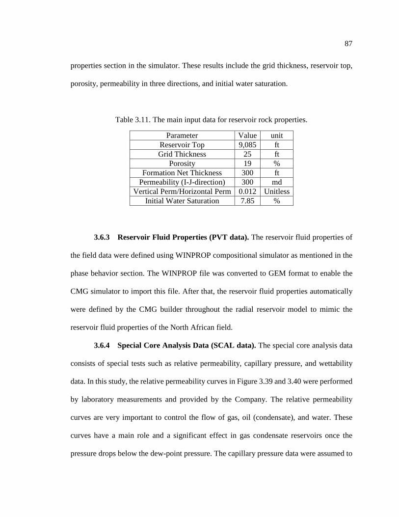
87
properties section in the simulator. These results include the grid thickness, reservoir top,
porosity, permeability in three directions, and initial water saturation.
Table 3.11. The main input data for reservoir rock properties.
Parameter Value unit Reservoir Top 9,085 ft Grid Thickness 25 ft
Porosity 19 % Formation Net Thickness 300 ft
Permeability (I-J-direction) 300 md Vertical Perm/Horizontal Perm 0.012 Unitless
Initial Water Saturation 7.85 %
3.6.3 Reservoir Fluid Properties (PVT data). The reservoir fluid properties of
the field data were defined using WINPROP compositional simulator as mentioned in the
phase behavior section. The WINPROP file was converted to GEM format to enable the
CMG simulator to import this file. After that, the reservoir fluid properties automatically
were defined by the CMG builder throughout the radial reservoir model to mimic the
reservoir fluid properties of the North African field.
3.6.4 Special Core Analysis Data (SCAL data). The special core analysis data
consists of special tests such as relative permeability, capillary pressure, and wettability
data. In this study, the relative permeability curves in Figure 3.39 and 3.40 were performed
by laboratory measurements and provided by the Company. The relative permeability
curves are very important to control the flow of gas, oil (condensate), and water. These
curves have a main role and a significant effect in gas condensate reservoirs once the
pressure drops below the dew-point pressure. The capillary pressure data were assumed to
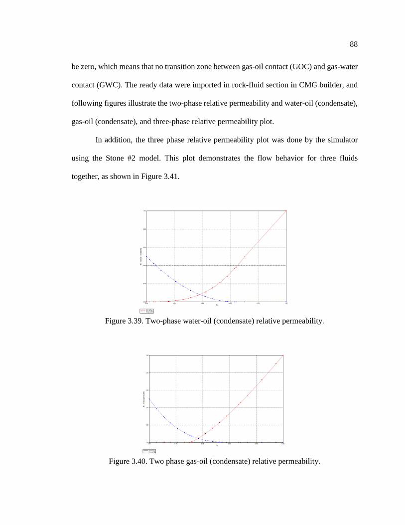
88
be zero, which means that no transition zone between gas-oil contact (GOC) and gas-water
contact (GWC). The ready data were imported in rock-fluid section in CMG builder, and
following figures illustrate the two-phase relative permeability and water-oil (condensate),
gas-oil (condensate), and three-phase relative permeability plot.
In addition, the three phase relative permeability plot was done by the simulator
using the Stone #2 model. This plot demonstrates the flow behavior for three fluids
together, as shown in Figure 3.41.
Figure 3.39. Two-phase water-oil (condensate) relative permeability.
Figure 3.40. Two phase gas-oil (condensate) relative permeability.

89
Figure 3.41. Three phase gas-oil (condensate)-water relative permeability.
3.6.5 Initial Conditions. This section is connected with the previous section, and
the parameters listed in Table 3.12 are essential to define in order to complete building the
model.
Table 3.12. Initial condition parameters.
Parameter Value unit Reference pressure (initial reservoir pressure) 3,740 psi
Reference depth (mid-perforation depth) 9,300 ft Water-Gas Contact (WOC) 9,585.5 ft
Water saturation below WOC 100 %
3.6.6 Wells and Recurrent Section. The well location was selected to be in the
center of the reservoir with Coordinates (1 1 1:20). The well was classified as a production
well and named Well-A-7. Also, the constraint values were added to the reservoir to
regulate the operation system. In addition, the date ranges were added, which the study
started in August 2005 to the target date in August 2050.

90
3.6.7 Numerical Section. This section is responsible for the solution iteration
time steps in order to have a smooth run and accurate results without warning messages.
Due to the complexity in gas condensate behavior, CMG support suggested that the
numerical solution section needs to modify the default values by changing the maximum
and minimum time step, linear solver iterations, linear solver orthogonalizations, and linear
solver factorization, as listed in Table 3.13. After this modification, the model runs
perfectly and shows results without any interruption during the run process.
Table 3.13. Numerical default and dataset values.
Parameter Default Value Dataset Value Max. Time Step Size 365 days 5 days Min. Time Step Size 1E-5 day 1E-6 day
3.6.8 Water Aquifer Properties. The bottom water aquifer was created based on
assumptions because the aquifer properties are unknown data. The correct data were known
after run the model and test the reservoir pressure history that affected directly by the water
aquifer model. Table 3.14 lists the first assumption iteration for the aquifer properties
Table 3.14. Data for the water aquifer properties.
Parameter Value unit Location Bottom - Thickness 750 ft Porosity 12 %
Permeability 70 md Radius 1,690 ft Angle 0.65 unitless
Modeling method Carter-Tracy - Leak Leakage is Allowed -

91
3.6.9 Reservoir Pressure History. The reservoir pressure history match was
affected by the water influx properties data and perforation completion (open or close) that
controls the water influx to avoid earlier invasion into the reservoir. Firstly, the water
aquifer properties were adjusted and run for multiple models. After that, the simulation
results were exported to an Excel spreadsheet file to plot with the reservoir pressure history
determined from the transient pressure analysis in 2009 and 2014, and other four points
provided by the company. From the plot, the simulation results were compared to the actual
pressure history. The perforation completion was changed by close or open the production
layer that closed to the Gas-Water-Contact (GWC). The model was run again, and the
results were exported to the same Excel sheet file. This step was repeated multiple times
until the best water influx model has approached. The final scenario represents the North
African water aquifer.
3.6.10 Gas, Condensate, and Water Production History. The production history
of the reservoir was impacted by the layer thickness. The first assumption was 9 ft for each
layer. However, the first scenario did not match the actual data. The decline in production
history started early due to the low potential energy of the reservoir. After the adjusting
process, the plateau period was longer as the layer thickness was increased until the match
was reached when the layer thickness was 25 ft.
3.6.11 Future Performance. After the match for the average reservoir pressure
had been reached, the projection of future IPR curve equations could be used to predict
North African field performance. The two methods that were used are the theoretical and
empirical methods. These techniques estimated the highest and lowest value of the absolute
open potential flow. The theoretical method was used first by using Equations 3.74 and

92
3.75 to predict the (𝑎𝑎) and (𝑏𝑏) values that changed during the operation life. Moreover,
the theoretical equation (Equation 3.70) was utilized to predict the new absolute open
potential flow value at a certain average reservoir pressure. The same procedures were
repeated for the empirical method, where inflow coefficient (𝐶𝐶) is determined using
Equation 3.76 and performance exponent (𝑛𝑛) is a constant value throughout the reservoir
life.
𝑎𝑎2 = 𝑎𝑎1 �
𝜇𝜇𝑔𝑔2 × 𝑍𝑍2𝜇𝜇𝑔𝑔1 × 𝑍𝑍1
� (3.74)
𝑏𝑏2 = 𝑏𝑏1 �
𝜇𝜇𝑔𝑔2 × 𝑍𝑍2𝜇𝜇𝑔𝑔1 × 𝑍𝑍1
� (3.75)
𝐶𝐶2 = 𝐶𝐶1 �
𝜇𝜇𝑔𝑔1 × 𝑍𝑍1𝜇𝜇𝑔𝑔2 × 𝑍𝑍2
� (3.76)
3.7 SENSITIVITY ANALYSIS
Sensitivity analysis techniques were utilized as part of reservoir simulation studies
in order to define the parameters that impact the reservoir pressure history, production
history for both gas and condensate, water cut, and gas recovery factor. This research
studied the following parameters.
3.7.1 Completion Perforation. This factor studied the effect of the production
interval on the reservoir performance and the effect of water aquifer on the production by
changing the location of perforation to produce far away from the gas-water-contact
(GWC). The sensitivity was done by changing from open status perforation to closed status

93
perforation to control the thickness of the production interval. The formation thicknesses
were chosen in the sensitivity analysis as follows: 250, 275, 325, and 350 ft.
3.7.2 Volume Lift Pressure Curve (VLP). Finally, after the IPR curves were
forecasted for several years, the sensitivity analysis in Prosper software was utilized to
predict the outflow tubing curve in order to estimate the flow rate system in the future. The
wellhead pressures were chosen for the sensitivity analysis as follows: 400 psi, 800 psi,
1,200 psi, 1,600 psi, and 2,000 psi.

94
4. RESULTS AND DISCUSSION
4.1 FORMATION EVALUATION OF THE FIELD
The target of using open-hole log interpretation techniques was to determine the
petrophysical properties for the North African field, where Figure 4.1 illustrates the main
results. The figure consists of three types of results: volume of shale, porosity, and
saturation through formation depths of 8,600 to 9,380 ft. As can be seen, the volume of
shale (represented by green) has a low trend between depths of 9,150 to 9,300 ft. This
represents the clean sand zone (limestone formation). At the same region, the porosity line
(shown in yellow) has an almost a constant value around 20%. In addition, the saturation
plot contains two scales of water and hydrocarbon saturation, where the water is
represented by blue and the hydrocarbon (gas) is represented by red. This plot indicates
that at the same interval, the hydrocarbon saturation is a high and water saturation is a low,
which represents the initial water saturation around 7%.
These results were converted to the Schlumberger’s Elan volume and Elan fluid in
order to obtain a clear understanding and deep details about the formation. Furthermore,
Figure 4.2 illustrates the Elan volume and Elan fluid for well A-7, where this figure assists
the interpreter to evaluate and detect the pay zone thickness and petrophysical properties.
The production interval is noticed clearly from both Elan plots, where the zone is between
depths of 9,090 to 9,330 ft. The Elan volume shows the volume of shale, volume of clean
sand (limestone formation), porosity, and water volume represented by gray, yellow, green,
and blue, respectively. On the other hand, the Elan fluid demonstrates the saturation of

95
water, movable hydrocarbon, and unmovable hydrocarbon, represented by blue, red, and
green, respectively.
Figure 4.1. The main calculations for the open-hole log interpretation.
The formation evaluation process concluded that the formation content
hydrocarbon has a good estimate, and the formation has very good bed thickness and
petrophysical properties. Moreover, the interpreter can visually read the average reservoir
porosity and average initial water saturation from the plot, or determine them from the cut-
off procedures as mentioned in Section 3, Part 1. Table 4.1 lists the results of average
reservoir porosity that is compatible to the result of the routine core analysis provided by

96
the company. The initial water saturation is approximately the same value as the special
core analysis data (relative permeability data).
Figure 4.2. Elan volume and Elan fluid for the well A-7.
Table 4.1. The results obtained from formation evaluation process.
Parameter Value Unit Formation net thickness 165 ft
Average reservoir porosity 0.19 fraction Average initial water saturation 0.0782 fraction
4.2 FLUID CHARACTERISTICS OF THE FIELD
Representative fluid is a crucial input for reservoir simulation studies, especially
for gas condensate case. In order to have a prober fluid model, a compositional simulation

97
model was established to match the gas condensate laboratory tests with the simulation
results. Figure 4.3 illustrates the constant volume depletion plot, which represents the
relationship between liquid volume (%) and pressure (psi). The dotted line shows the initial
assumption step that was modulated by the simulator. As seen in the figure, the trend of
the bold line indicates that the match was achieved by the final simulation run. This line
was matched the experimental points perfectly and was thus taken as a representative of
the fluid of the North African field. The simulator mimicked the reservoir fluid behavior
in order to have accurate studies for the North African condensate fluid phenomena. The
simulation results achieved dew-point pressure that was approximately the same value as
the PVT data report, which is around 3,656.4 psi at the reservoir temperature 285˚F.
Furthermore, the maximum liquid dropout was determined to be around 1% at reservoir
pressure 1,700 psi.
Figure 4.3. Constant volume depletion (CVD) model.

98
On the other hand, Figure 4.4 demonstrates the constant composition expansion
plot, which represents the relationship between relative volume (fraction) and pressure
(psi). The dotted line in this plot represents the initial assumption step that was
automatically performed by the simulator. After regression process, the final match was
reached at the dew-point pressure of 3,656.4 psi represented by the bold line. Therefore,
the matching line is laying perfectly on the experimental points.
Figure 4.4. Constant composition expansion (CCE) model.
The phase envelope diagram was performed as illustrated in Figures 4.5 and 4.6,
where the pressure-temperature plot represents the phase behavior of the North African
field at the isothermal condition (reservoir temperature is constant throughout the
reservoir). Figure 4.5 shows a wide range of the liquid volume between quality lines that
is every 1%. As seen in the figure, when pressure drops below the dew point pressure at

99
the reservoir temperature 285˚F, the liquid starts evolving from the gas phase until reaching
the maximum value of the liquid dropout at 1% liquid volume at the reservoir pressure
1,700 psi. These results are compatible with the constant volume depletion test results,
constant composition expansion outcomes, and the laboratory measurements.
In order to investigate the amount of liquid dropout at a narrow range of pressures,
the quality lines were performed to be every 0.1%, as shown in Figure 4.6. Moreover, it
can be noticed that the quality lines are close to each other approximately every 150 psi
pressure drop. As a result, the liquid dropout is increased by 0.01% liquid volume. These
results are the crucial factor in order to investigate and understand the behavioral change
in this case using the reservoir simulation technique.
Figure 4.5. Phase envelope diagram for the gas condensate reservoir with 1% liquid
volume ranges between the quality lines.
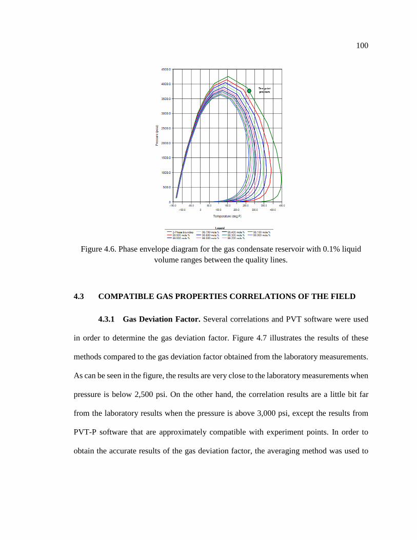
100
Figure 4.6. Phase envelope diagram for the gas condensate reservoir with 0.1% liquid
volume ranges between the quality lines.
4.3 COMPATIBLE GAS PROPERTIES CORRELATIONS OF THE FIELD
4.3.1 Gas Deviation Factor. Several correlations and PVT software were used
in order to determine the gas deviation factor. Figure 4.7 illustrates the results of these
methods compared to the gas deviation factor obtained from the laboratory measurements.
As can be seen in the figure, the results are very close to the laboratory measurements when
pressure is below 2,500 psi. On the other hand, the correlation results are a little bit far
from the laboratory results when the pressure is above 3,000 psi, except the results from
PVT-P software that are approximately compatible with experiment points. In order to
obtain the accurate results of the gas deviation factor, the averaging method was used to

101
determine the average gas deviation factor from these methods. Figure 4.8 shows the
average gas deviation factor compared to the experiment gas deviation factor.
Figure 4.7. Results of gas deviation factor using different methods.
Figure 4.8. Comparison between gas deviation factor from the laboratory measurements
and averaging value from different methods.

102
As shown in the figure, the formula obtained from the trend line was utilized to
obtain the accurate gas deviation gas factor and then used for the pseudo-gas potential
pressure calculations.
4.3.2 Gas Viscosity. Figure 4.9 illustrates the Lee, Gonzalez, and Eakin
correlation results of the gas viscosity versus pressure. The figure indicates that the gas
viscosity increased as the reservoir pressure increased. The trend line was plotted in order
to obtain the gas viscosity formula and was utilized to determine the gas viscosity for wide
range of pressures. These results were used with gas deviation factor results to estimate the
real gas pseudo-pressure for the reservoir fluid.
Figure 4.9. Relationship between gas viscosity using Lee, Gonzalez, and Eakin
correlation and pressure.
4.3.3 Isothermal Compressibility. As the reservoir pressure increases the
isothermal compressibility decreases until reaching a certain pressure that will be almost a
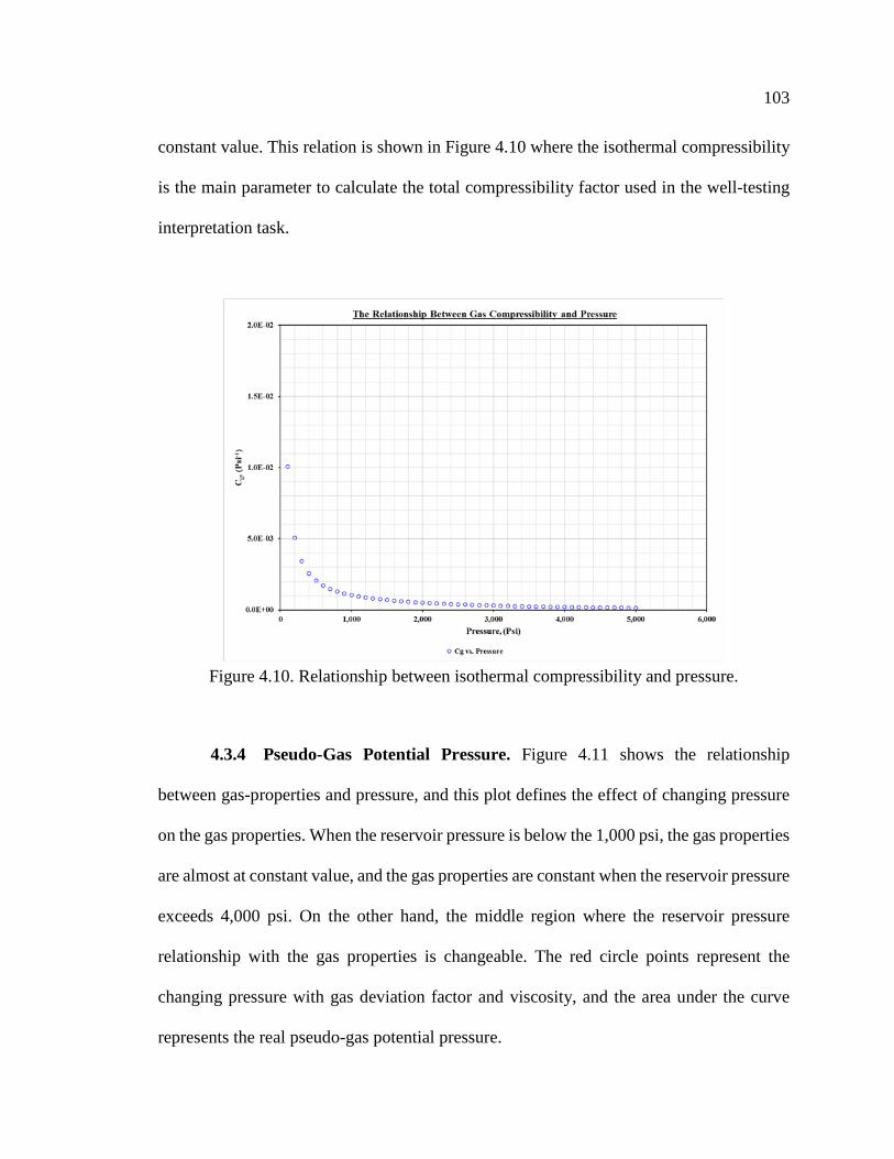
103
constant value. This relation is shown in Figure 4.10 where the isothermal compressibility
is the main parameter to calculate the total compressibility factor used in the well-testing
interpretation task.
Figure 4.10. Relationship between isothermal compressibility and pressure.
4.3.4 Pseudo-Gas Potential Pressure. Figure 4.11 shows the relationship
between gas-properties and pressure, and this plot defines the effect of changing pressure
on the gas properties. When the reservoir pressure is below the 1,000 psi, the gas properties
are almost at constant value, and the gas properties are constant when the reservoir pressure
exceeds 4,000 psi. On the other hand, the middle region where the reservoir pressure
relationship with the gas properties is changeable. The red circle points represent the
changing pressure with gas deviation factor and viscosity, and the area under the curve
represents the real pseudo-gas potential pressure.
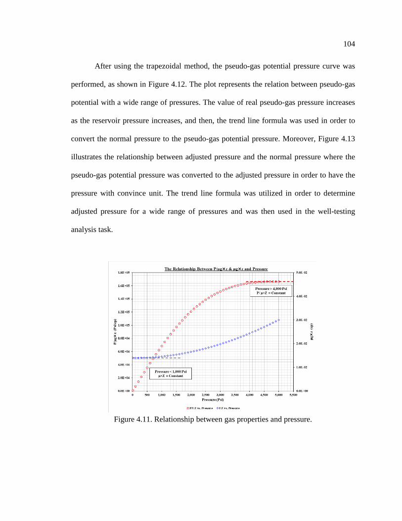
104
After using the trapezoidal method, the pseudo-gas potential pressure curve was
performed, as shown in Figure 4.12. The plot represents the relation between pseudo-gas
potential with a wide range of pressures. The value of real pseudo-gas pressure increases
as the reservoir pressure increases, and then, the trend line formula was used in order to
convert the normal pressure to the pseudo-gas potential pressure. Moreover, Figure 4.13
illustrates the relationship between adjusted pressure and the normal pressure where the
pseudo-gas potential pressure was converted to the adjusted pressure in order to have the
pressure with convince unit. The trend line formula was utilized in order to determine
adjusted pressure for a wide range of pressures and was then used in the well-testing
analysis task.
Figure 4.11. Relationship between gas properties and pressure.

105
Figure 4.12. Relationship between pseudo-gas potential pressure and pressure.
Figure 4.13. Relationship between adjusted pressure and pressure.

106
4.4 RESERVOIR CHARACTERISTICS OF THE FIELD
4.4.1 Analytical Method Results. The modern key result of the well-testing
interpretation is the pressure derivative plot that represents the relationship between the
Bourdet pressure derivative in red and pseudo-gas potential pressure drop in blue in y-axis
versus the shut-in time in the x-axis, as illustrated in Figure 4.14. The early time as can be
seen in the figure indicates that the wellbore storage region is varying. In this case, the
wellbore storage is changing wellbore storage behavior due to a decrease in the fluid
compressibility in the wellbore and tubing production. This happens in gas wells that have
a high gas-oil ratio. When the well is shut-in, the liquid falls down in the borehole. This
causes a change in density between gas and liquid and fluid and then a decrease in the
pressure for a period of time. The middle time represents the porous media through the
reservoir formation, and this case has three stabilization regions (radial flow regions). As
can be seen in the figure, the pressure derivative behavior is decreased down as stairs, and
this indicates that the reservoir fluid mobility ratio is changing throughout the reservoir.
As the flow goes through the wellbore region, the reservoir permeability is decreased due
to the decrease gas mobility ratio and increasing liquid amount in the porous media. As
shown in the figure, the stabilization equation indicates that as the stabilization period is
small, the permeability and net formation thickness values are high. On the other hand, the
gas viscosity is low due to change the fluid behavior in the North African reservoir. Finally,
the late time demonstrates the boundary effect that is not shown clearly in the derivative
points. However, the late period in the pressure drop points have little stabilization, which
indicates the reservoir is under the water aquifer (constant boundary).

107
Figure 4.14. Pressure derivative plot for the buildup test.
The superposition plot approach was performed with the pressure derivative to
detect the radial flow region in each stabilization period, as shown in Figure 4.15, 4.16,
and 4.17. The red line represents the pressure derivative and the blue line is the pseudo-
potential pressure drop. In each stabilization region, the slope was taken in order to obtain
the formula, and then the reservoir characteristics values were determined.
Figure 4.15. Superposition plot for the first radial flow regions.

108
Figure 4.16. Superposition plot for the second radial flow regions.
Figure 4.17. Superposition plot for the third radial flow regions.
Table 4.2 lists the results of the three regions. As seen in the table, the permeability
value at the first region is lower than the second and third. Furthermore, the skin factor has
a negative sign when the formation closes the wellbore region, and this indicates that an

109
acidizing job was done to the well after drilling operation. Finally, reservoir characteristic
values indicate that the formation has good properties and decreasing in permeability is
due to a change in the mobility ratio that causes the liquid dropout during the pressure
drawdown.
Table 4.2. Well-testing interpretation results for three radial flow regions using superposition plot.
Parameter First Region
Second Region
Third Region Unit
Slope 2.2674E+06 1.6667E+06 1.0867E+06 Psi2/cp/Cycle
Formation Flow Capacity 23,021 31,318 48,032 md.ft
Permeability 142.10 193.32 296.49 md
Intercept 6.5655E+08 6.5426E+08 6.5254E+08 Psi2/cp
P1hr 6.4855E+08 6.4838E+08 6.4871E+08 Psi2/cp
Total Skin -1.98 -0.51 3.05 -
4.4.2 Type Curve Results. Gringarten type curve analysis was utilized for more
confident interpretation results. This method includes more results related to the wellbore
storage outcomes. Table 4.3 lists the permeability and skin factor results for the three
regions, which are very close to the superposition plot method outcomes. Because the
wellbore storage results are not the same value for three regions, commercial software was
used in order to obtain accurate results.

110
Table 4.3. Well-testing interpretation results for three radial flow regions using
Gringarten type curve.
Parameter First Region Second Region Third Region Unit
Ca 5.495 5.495 5.495 Rbbl/Psi
CDe2s 1.E+02 2.E+03 3.E+06 -
k 142.27 197 292 md
Kh 23,049 31,836 47,269 md.ft
CaD 6,292 5,215 6,046 -
Ca 4.864 4.031 4.674 Rbbl/Psi
S' -2.07 -0.53 3.03 -
4.4.3 Modern Method Results. Saphir software was used for deep interpretation
in order to obtain more results about the reservoir. Figure 4.18 illustrates the pressure
derivative for the buildup test, where the small black line represents the software model,
and the red and green points represent the pressure derivative and gas potential pressure
drop for the field data. The software shows that the early time has changing wellbore
storage due to change in the fluid compressibility. This region was matched using the
Hegeman wellbore model, which is recommended by Kappa Engineering. Moreover, in
order to match the middle region (reservoir model), multiple models were tried until the
match was achieved using the radial composite model. The plot shows that the reservoir
model is a radial composite model with three regions, and due to the software limitation,
only the second and the third regions were matched perfectly, and the model did not match
the first region, as shown in Figure 4.18.
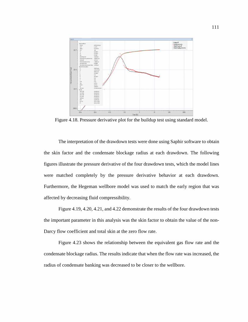
111
Figure 4.18. Pressure derivative plot for the buildup test using standard model.
The interpretation of the drawdown tests were done using Saphir software to obtain
the skin factor and the condensate blockage radius at each drawdown. The following
figures illustrate the pressure derivative of the four drawdown tests, which the model lines
were matched completely by the pressure derivative behavior at each drawdown.
Furthermore, the Hegeman wellbore model was used to match the early region that was
affected by decreasing fluid compressibility.
Figure 4.19, 4.20, 4.21, and 4.22 demonstrate the results of the four drawdown tests
the important parameter in this analysis was the skin factor to obtain the value of the non-
Darcy flow coefficient and total skin at the zero flow rate.
Figure 4.23 shows the relationship between the equivalent gas flow rate and the
condensate blockage radius. The results indicate that when the flow rate was increased, the
radius of condensate banking was decreased to be closer to the wellbore.
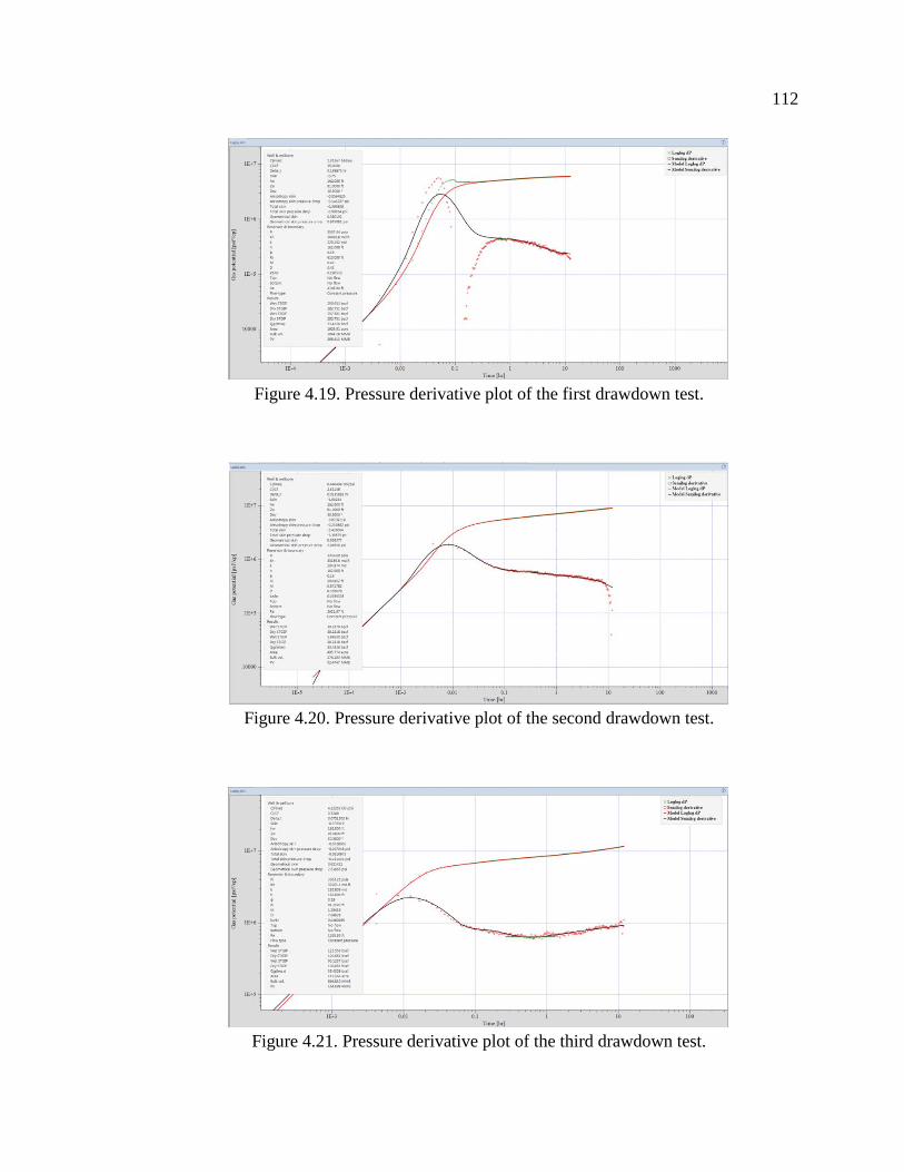
112
Figure 4.19. Pressure derivative plot of the first drawdown test.
Figure 4.20. Pressure derivative plot of the second drawdown test.
Figure 4.21. Pressure derivative plot of the third drawdown test.

113
Figure 4.22. Pressure derivative plot of the fourth drawdown test.
Figure 4.23. The relationship between equivalent gas flow rate and composite radius.
4.4.4 Dependent Skin Results. Figure 4.24 represents the rate-dependent skin
method that was utilized to have a perfect match for the reservoir pressure history
throughout the test. As can be seen in the plot, the intercept represents the skin factor at the
zero flow rate and the slope represents the non-Darcy flow coefficient.

114
Figure 4.24. The initial results of the rate-dependent skin method.
These results that obtained from Figure 4.25 are the main effective parameters to
achieve the pressure history match. Figure 4.26 shows the results after the regression
process, the model matched the reservoir pressure history perfectly. The accurate skin
factor at the zero flow rate, the non-Darcy flow rate, and the average reservoir pressure
were obtained to be used in the deliverability calculations.
Figure 4.26 illustrates the results of the rate-dependent skin method after obtaining
the skin factor from each drawdown using the time-dependent skin method. The time-
dependent skin method was used to compare the results with the rate-dependent skin
method to confirm the results of skin factor at the zero flow rate, the non-Darcy flow
coefficient, and average reservoir pressure. As a result, the outcomes were very close in
both methods, but the model line of the second method in the pressure history plot had the
better match, as shown in Figure 4.27. This plot shows the results that were used in the
deliverability analysis and reservoir simulation studies.

115
Figure 4.25. The pressure history match though the test using the rate-dependent skin
method.
Figure 4.26. The results of the rate-dependent skin method.
Figure 4.27. The pressure history match though the test using the time-dependent skin
method.

116
4.4.5 Comparison Between Two Tests. The pressure derivative overlay was
used to compare the pressure derivative for both the well tests in 2009 and 2014, as
illustrated in Figure 4.28. As seen in the plot, both pressure derivatives have the same
shape, where the three radial flow regions can be noticed. The changing in the wellbore
storage exists in both pressure derivatives. Thus, all the results in both tests are
approximately compatible, and slight change in the outcome values were due to changing
in mobility ratio as a result, pressure depletion and increasing in the liquid dropout.
Figure 4.28. The pressure derivative overlay for the buildup tests in 2009 and 2014.
4.5 THE FIELD FLOW POTENTINAL
The results that illustrated in this section were obtained from the analysis of the
flow-after-flow test in 2009.
4.5.1 Analytical Results. An empirical method was used using three techniques
(Excel, Saphir, and Prosper) to obtain the empirical parameters, the inflow, and outflow

117
reservoir performance. Figure 4.29 illustrates the empirical method analysis using Excel
calculations. The analysis shows that the performance exponent value is around 0.80
(unitless) which indicates the reservoir is under the condition flow closest to the laminar
flow. The non-Darcy flow coefficient from the well-testing interpretation in 2009 was a
very low value that proved there is no turbulent flow during the production process. This
allows the reservoir potential to be very high, as found using the empirical method where
the absolute open flow (AOF) potential in 2009 was around 985.34 MMscf/day.
Figure 4.29. Deliverability analysis using the empirical method with the Excel.
Furthermore, the empirical method was utilized using Prosper software, and this
method in the software is known as a multi-rate (𝐶𝐶) and (𝑛𝑛) method. Figure 4.30 illustrates
the IPR curve and the main results are listed in the box inside the plot. These parameters
are the same as previous approaches.

118
The software was selected to build the vertical lift performance with the IPR of the
well in the North African field. Figure 4.31 shows the match of the outflow performance
with inflow performance curve. The intersecting point between the two lines represents the
gas flow rate system. This is the flow rate that the well can produce when the well-head
pressure is 2,196 psi.
Figure 4.30. The empirical inflow performance relationship using Prosper.
Figure 4.31. Match of vertical lift performance with the empirical inflow performance
relationship using Prosper software.

119
Theoretical method is based on the pressure square approach that was utilized to
obtain the theoretical parameters and the inflow and outflow performance of the reservoir
using three applications: Excel and Prosper. Figure 4.32 shows the analysis to determine
the theoretical parameters obtained from the trend line formula. These parameters were
used to determine the AOF potential. This approach indicates that the reservoir potential is
high as proved in the previous method, and the value of AOF is around 510 MMscf/day.
This technique shows that the value of AOF is lower than the AOF from the empirical
method due to the assumption in each method.
Figure 4.32. Deliverability analysis using the theoretical method with Excel.
This approach is known in Prosper by name the multi-rate Jones. As shown in
Figure 4.33, the deliverability results for this method are the same as the previous technique
(Excel). The plot shows the results where these parameters were used to perform the IPR
curve.

120
Figure 4.33. The theoretical inflow performance relationship using Prosper.
The same well-head pressure value was used in the Prosper software to obtain the
gas flow rate system for the well using the theoretical method. The vertical lift performance
was performed on the inflow performance plot, as shown in Figure 4.34, where the value
of the gas flow rate system was around 65 MMscf/day. The result from this plot is the same
as in the empirical method.
Figure 4.34. Match of vertical lift performance with the theoretical inflow performance
relationship using Prosper software.

121
The assumption of the exact method is based on the real gas pseudo-pressure that
was used to count the effect of the gas properties change with respect to pressure. This
method was calculated using Excel calculations, Saphir, and Prosper. Figure 4.35 shows
the results of this technique using the Excel, and the absolute open flow (AOF) potential
was around 566 MMscf/day. This value is very close to the theoretical AOF, but the value
of the exact AOF is lower than the empirical AOF.
Figure 4.35. Deliverability analysis using the exact method with Excel.
Prosper shows the same results as the previous tools (Excel), where the exact
parameter results are listed in Figure 4.36. The IPR curve is illustrated in the figure using
the exact method, which is called the multi-rate Forchheimer with pseudo-pressure.

122
Figure 4.36. The exact inflow performance relationship using Prosper.
Figure 4.37 illustrates the vertical lift performance for the well where the
intersecting point between the two models was around 65 MMscf/day. This value
represents the gas flow rate system of the well in the North African field.
Figure 4.37. Match of vertical lift performance with the exact inflow performance
relationship using Prosper.

123
As can be seen in Figure 4.38, the gas flow rate system is a constant value in three
methods, but the absolute open flow (AOF) potential in each method has a difference value
due to the different in equation assumptions.
Figure 4.38. Match of vertical lift performance with the three inflow performance
relationship methods using Prosper software.
4.5.2 Explanation of Results. The key factor to understand the difference in the
absolute open flow potential results in the three methods is shown in Figure 4.39. When
the pressure is below the 1,000 psi, the empirical method is valid due to the gas properties
remaining constant with the changing pressure. The exact method works when the pressure
ranges between 1,500 to 4,000 psi, as shown in the plot. This area shows that the gas
properties have a large change with changing pressure. The late region represents the
theoretical method area that is valid when the pressure is above 4,000 psi. According to
Johnston et al., in 1991 SPE 23440, using the empirical method (Rawlins and Schellhardt)
could cause an incorrect value of absolute open flow potential due to over large variations

124
in pressure when extrapolate the empirical equation. In addition, the empirical equation is
valid only in low pressure ranges (Lee, 1982).
Figure 4.39. Relationship between gas properties with pressure.
Figure 4.40. Modified empirical equation results.

125
In order to decrease the error in the empirical equation, the equation was modified
by replacing the normal pressure with the pseudo-gas pressure in Equation 3.68. Figure
4.40 shows the results in the new empirical equation, where the absolute open flow (AOF)
potential is very close to the AOFs in the theoretical and exact method. The exponent
performance is almost the same as exponent performance in the normal empirical equation.
According to Lee, Well Testing SPE book in 1982, this equation is applicable for wide
range of pressures when the gas pseudo-pressure is used.
Figure 4.41 illustrates the inflow performance relationship with the vertical lift
performance curve using the modified empirical equation.
Figure 4.41. Match of vertical lift performance with the modified empirical inflow
performance relationship using Prosper.
Figure 4.42 illustrates the inflow performance relationship with the vertical lift
performance curve using all methods, where the difference in AOF values is shown clearly.

126
Figure 4.42. Match of vertical lift performance with all methods of the inflow
performance relationship using Prosper.
4.5.3 Comparison between Two Tests. Figure 4.43 illustrates the empirical
method calculations in 2009 and 2014 where test data shows the empirical method
parameters for the different years. This relationship proves that the performance exponent
(𝑛𝑛) is constant through two tests, where the value is around 0.81 (unitless). Subsequently,
the performance exponent is a constant value in future analysis. On the other hand, the
inflow coefficient (𝐶𝐶) was slightly increased from 2009 to 2014. As a result, the (AOF)
potential was decreased by 3.38% during that time.
Furthermore, the IPR curve was performed in 2009 and 2014, as shown in Figure
4.44. This plot shows the effect of the new AOF and of C on the IPR curve, where the
curve in 2014 shift down due to the reduction in AOF.

127
Figure 4.43.Empirical method calculations in 2009 and 2014.
Figure 4.44. Empirical inflow performance relationship in 2009 and 2014.
Figure 4.45 and 4.46 show the IPR curve in both methods (theoretical and exact).
The well performance was reduced as the years increased. The down shift in the IPR curve
in 2014 was due to the change in the main parameters that built the two techniques. The

128
decrease in the AOF value in the theoretical method was around 1.71% and approximately
2.84% in the exact method.
Figure 4.45. Theoretical inflow performance relationship in 2009 and 2014.
Figure 4.46. Exact inflow performance relationship in 2009 and 2014.

129
4.6 SIMULATION OUTCOMES OF THE FIELD
This section represents the base case for the North African simulation model. The
case was built based on the previous tool results in order to mimic the field. Figure 4.47
illustrates the average reservoir pressure history simulation results over the years.
Figure 4.47. Reservoir average pressure history result using reservoir simulation.
As shown in Figure 4.48, the pressure curve is curved and shifted up when the water
starts invading the reservoir approximately in the year 2022. This indicates that the water
cut support the average reservoir history and prevents the early depletion in the reservoir
pressure. In other words, the relationship is proportional when the water cut is increased
and the reservoir pressure is more supported. The water cut in this case is very low, which
is slowly increased over the years, and the ultimate water cut value in 2050 is less than
0.05.

130
Figure 4.48. Relationship between reservoir average pressure and water cut simulation
history.
Figure 4.49 illustrates the reservoir simulation results that match the results of the
well-testing data points. In order to have a perfect match for the average reservoir pressure,
the aquifer data were modified using trial and error techniques. Table 4.4 lists the final
results that represent the North African aquifer data.
Table 4.4. The water aquifer properties data.
Parameter Value unit Location Bottom - Thickness 1,000 ft Porosity 15 %
Permeability 220 md Radius 8,600 ft Angle 0.85 Unitless
Modeling method Carter-Tracy - Leak Leakage is allowed -
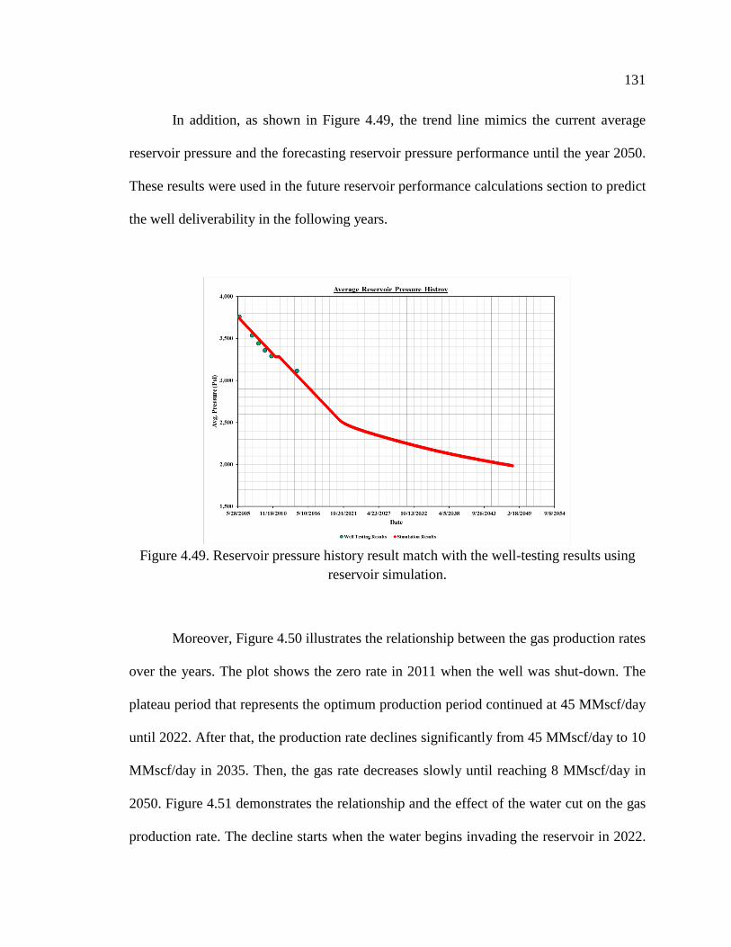
131
In addition, as shown in Figure 4.49, the trend line mimics the current average
reservoir pressure and the forecasting reservoir pressure performance until the year 2050.
These results were used in the future reservoir performance calculations section to predict
the well deliverability in the following years.
Figure 4.49. Reservoir pressure history result match with the well-testing results using
reservoir simulation.
Moreover, Figure 4.50 illustrates the relationship between the gas production rates
over the years. The plot shows the zero rate in 2011 when the well was shut-down. The
plateau period that represents the optimum production period continued at 45 MMscf/day
until 2022. After that, the production rate declines significantly from 45 MMscf/day to 10
MMscf/day in 2035. Then, the gas rate decreases slowly until reaching 8 MMscf/day in
2050. Figure 4.51 demonstrates the relationship and the effect of the water cut on the gas
production rate. The decline starts when the water begins invading the reservoir in 2022.

132
The plot proves that the relationship is an inverse relationship, and the water has a negative
impact on the gas production rate.
Figure 4.50. Gas production rate simulation history.
Figure 4.51. The relationship between the gas production rate and water cut simulation
history.
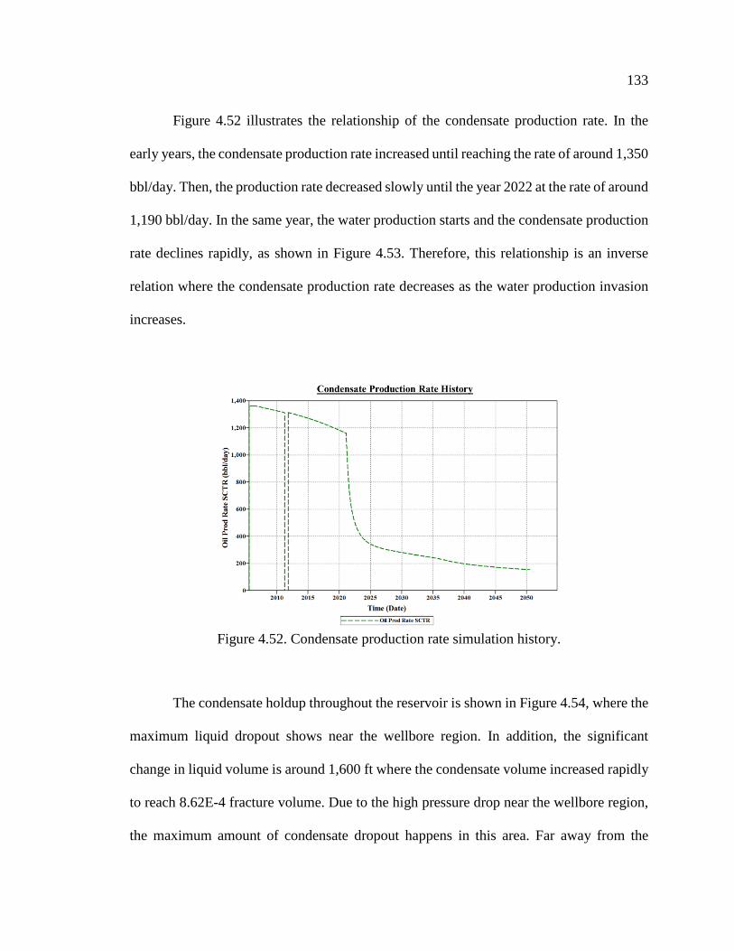
133
Figure 4.52 illustrates the relationship of the condensate production rate. In the
early years, the condensate production rate increased until reaching the rate of around 1,350
bbl/day. Then, the production rate decreased slowly until the year 2022 at the rate of around
1,190 bbl/day. In the same year, the water production starts and the condensate production
rate declines rapidly, as shown in Figure 4.53. Therefore, this relationship is an inverse
relation where the condensate production rate decreases as the water production invasion
increases.
Figure 4.52. Condensate production rate simulation history.
The condensate holdup throughout the reservoir is shown in Figure 4.54, where the
maximum liquid dropout shows near the wellbore region. In addition, the significant
change in liquid volume is around 1,600 ft where the condensate volume increased rapidly
to reach 8.62E-4 fracture volume. Due to the high pressure drop near the wellbore region,
the maximum amount of condensate dropout happens in this area. Far away from the

134
wellbore region, the liquid dropout is an almost constant value. Also, this is proved using
a well-testing interpretation tool that showed the condensate blockage is around the
wellbore region. Figure 4.55 illustrates the change in condensate volume fracture over the
years where the maximum amount is around 0.55 in 2055 in a distance of around 700 ft.
This proves that the condensate volume increases as the average reservoir pressure
decreases, which causes an increase in the pressure drop over the years.
Figure 4.53. The relationship between the condensate production rate and water cut
simulation history.
Figure 4.56 shows the 3-D model for the reservoir, which illustrates the water cut
movement throughout the reservoir layers over the years. As shown, the three bottom layers
will be completely filled with the water in 2055, and the water cut will reach 0.60 at the
fourth layer. Therefore, this movement of water from the aquifer to the reservoir depends
on the vertical permeability of the reservoir.

135
Figure 4.54. Condensate dropout throughout the reservoir radius.
Figure 4.55. Condensate dropout over the years.
Figure 4.56. Water cut over years.

136
4.7 FUTURE FLOW PERFORMANCE OF THE FIELD
4.7.1 Applicability of Equations. The modified empirical method was tested to
investigate the applicability of the equation results with the well deliverability analysis in
the 2009 and 2014 outcomes. Table 4.5 shows the prediction results of the AOF using the
modified empirical method. The results indicate that the equation is applicable for this case,
and the relative error did not exceed 4% in the inflow coefficient. On the other hand, the
absolute open flow (AOF) potential has a high error value which is around 10%, as seen in
Table 4.6.
Table 4.5. The equation applicability in the modified empirical method.
Pressure Psi
𝐶𝐶 from Equation
MMScf/day/Psi2
AOF from Deliverability MMScf/day
AOF from Equation
MMScf/day 3,117.13 2.844E-12 636.484 571.103
Table 4.6. Relative error results for the modified empirical method calculations.
Parameter Relative Error, (%) 𝐶𝐶 3.75
AOF 10.272
The theoretical method was also tested to investigate the error in Equation 3.73 and
3.74, as mentioned in Section 3. Table 4.7 demonstrates the results of the prediction the
AOF and the theoretical parameters. Furthermore, Table 4.8 shows the relative error where
the error value was around 7 % for the theoretical parameters. Although the relative errors

137
for the input values are somewhat high, the relative error that was determined from the
absolute open flow (AOF) potential did not exceed 0.03 %, as seen in Table 4.9.
Table 4.7. The equation applicability in the theoretical method.
Pressure Psi
𝑎𝑎 from Equation Psi2/MMScf
/day
𝑏𝑏 from Equation (Psi/MMScf
/day)2
AOF from Deliverability MMScf/day
AOF from Equation
MMScf/day 3,117.13 3,949.38 33.49 501.60 501.482
Table 4.8. Relative error results for the theoretical method calculations.
Parameter Relative Error, (%) 𝑎𝑎 5.06 𝑏𝑏 7.5
AOF 0.024
4.7.2 Application of the Equations. Table 4.9 shows the final results of the
AOFs empirical method that were predicted in 2014, 2018, and 2050. These values are
shown graphically in Figure 4.57. As the reservoir pressure is depleted, the IPR curve is
shifted down over the years, and this causes the production productivity to reduce.
Table 4.9. The prediction results of the IPR parameters.
Average Reservoir Pressure Psi
Date MM/DD/YYYY
𝐶𝐶 MMScf/day/Psi2
AOF MMScf/day
3,117.13 06/01/2014 2.844E-12 571.10 2,780.56 02/01/2018 3.038E-12 444.67 1,954.85 08/01/2050 3.510E-12 183.764

138
Figure 4.57. Predicting the IPR curves using the modified empirical method.
Finally, Table 4.10 lists the final results of the AOFs theoretical method that were
predicted in 2014, 2018, and 2050. In addition, Figure 4.58 illustrates these results on the
IPR curves that represent the performance of the reservoir in the future. As seen in the
figure, the IPR curves are shifted down due to a decrease in the average reservoir pressure
that caused the well performance productivity to reduce.
Table 4.10. The prediction results of the IPR parameters.
Average Reservoir Pressure
Psi
Date MM/DD/YYYY
𝑎𝑎 from Equation
Psi2/MMScf /day
𝑏𝑏 from Equation
(Psi/MMScf /day)2
AOF MMScf/day
951.241 06/01/2014 3,759.00 31.14 501.48 2,780.56 02/01/2018 3,697.34 31.36 441.07 1,954.85 08/01/2050 3,200.52 27.14 320.85

139
Figure 4.58. Predicting the IPR curves using the theoretical method.
4.7.3 Future Scenarios for Matching VLP with IPR. As shown in Figure 4.59
and 4.60, the wellhead pressure that is required to lift the hydrocarbon to the surface is
decreased and shifted down as the average reservoir pressure decreases. All the volume lift
pressure (VLP) pressures assumptions are matched with the IPR curves in 2009, 2014, and
2018. On the other hand, the IPR curve in 2050 is matched only with the VLP pressure at
1,200 psi and below. The gas flow rate system is increased as the wellhead pressure
decreased where the range of the gas flow rate system is between 40 to 100 MMscf/day.
The gas flow rate system results are almost the same in both methods, which proves that at
the low pressure, both methods have the same result in the IPR and VLP curves. Finally,
the difference in both methods is in the AOF value where the empirical method is the
optimistic technique, and the theoretical method is the conservative technique.

140
Figure 4.59. Predicting the match of VLP with the empirical IPR curves.
Figure 4.60. Predicting the match of VLP with the theoretical IPR curves.

141
4.8 DEVELOPMENT STRATEGY PLAN OF THE FIELD
In order to improve the gas recovery factor and to study the water cut effect, the
development strategy plan was based on Figure 4.61. This figure represents the formation
and well schematic of the North African field where the formation top is at a depth of
9,085.5 ft and the gas-water contact is at a depth of 9,435.5 ft. In addition, the total pay
zone thickness is 350 ft, and each layer has a 25 ft thickness. Also, the North African water
aquifer is shown in blue, which is classified as a bottom water drive with a 1,000 ft
thickness. The strategy was done by closing the lower layers to avoid early water invasion
into the reservoir.
Figure 4.61. The North African formation schematic.
Figure 4.62 illustrates the relationship of the water cut history for different strategy
plans over the years. The results indicate that when the pay zone thickness is opened
completely, the water starts moving into the reservoir early. As shown in Figure 4.62, the
dark blue case with a 350 ft thickness has a significantly higher water cut than the other
cases.

142
Figure 4.62. Water cut sensitivity results over the years.
In addition, Figure 4.63 shows the relationship of the gas production rate history
over the years where the thickness has the main effect on the plateau period before the gas
production rate starts declining. When the pay zone thickness is high, the gas production
decline starts earlier. As shown in Figure 4.63 and 4.64, this happens due to the water influx
into the reservoir where the water drive has a negative impact on the gas production rate.
Figure 4.63. Gas production rate sensitivity results over the years.
Also, the gas recovery factor is affected by the formation thickness where the lower
thickness results in a higher gas recovery factor, as shown in Figure 4.64. The main reason

143
that affected the gas recovery is the water cut. These is a higher gas recovery factor, the
reservoir has a lower water cut.
Figure 4.64. Gas recovery factor sensitivity results over the years.
Moreover, the result details are listed in Table 4.11, which includes the water cut
history and the gas recovery factor for every 10 years at each pay zone thickness case. As
shown, the water cut increases gradually over the years, especially in a large thickness
formation. However, the gas recovery factor decreases as the water cut increases.
Furthermore, this impacts the gas recovery factor, which is reduces by 43.3% in 2040 from
the 250 ft to 350 ft thickness cases. The base case gas recovery factor is increased by
24.37% in 2040 compared to the 350 ft thickness case. On the other hand, the base case
water influx is reduced by 0.01 (fraction) in 2040 compared to the 350 ft thickness case.
Table 4.12 shows the final results in 2050 where the water cut reaches a high value
of around 0.0267 (fraction) at the 350 ft thickness case. However, at the same year and
thickness, the gas recovery factor is around 25.82%, which is lower by 46.63% compared
to the 250 ft thickness case.

144
Table 4.11. The results of the formation thickness sensitivity.
Thickness Ft
Date MM/DD/YYYY
Water Cut Fraction
Recovery Factor %
350
08/01/2010 0.00039 10.44 08/01/2020 0.01545 18.31 08/01/2030 0.0217 21.21 08/01/2040 0.025 23.56
325
08/01/2010 0.00026 10.44 08/01/2020 0.0091 27.19 08/01/2030 0.0142 32.20 08/01/2040 0.0184 35.81
300 (Base Case)
08/01/2010 0.00026 10.44 08/01/2020 0.00053 32.68 08/01/2030 0.0105 42.64 08/01/2040 0.015 47.93
275
08/01/2010 0.00025 10.44 08/01/2020 0.00033 32.68 08/01/2030 0.0091 51.78 08/01/2040 0.01273 58.20
250
08/01/2010 0.00025 10.44 08/01/2020 0.00033 32.68 08/01/2030 0.00058 56.32 08/01/2040 0.01270 66.86
Table 4.12. The final results of the formation thickness sensitivity in the target year.
Date MM/DD/YYYY
Thickness Ft
Water Cut Fraction
Recovery Factor %
8/1/2050
350 0.0267 25.82 325 0.0211 39.05 300
(Base Case) 0.0191 52.12
275 0.0180 63.33 250 0.0168 72.45

145
5. CONCLUSIONS & RECOMMENDATIONS
5.1 CONCLUSIONS
1. The open-hole log analysis indicates that the formation has lower shale value where
GR log reading is below 25 GAPI. In addition, the sonic log line trend is almost
constant throughout the target zone, which indicates that the reservoir has consistent
lithology. Moreover, the separation between resistivity readings refers to the
hydrocarbon zone. Furthermore, the initial water saturation is very low at around 7%,
and the formation fills with a high amount of hydrocarbon.
2. Elan volume and Elan fluid plots show deep and more detailed information about the
North African formation, which is crucial in order to detect the bed formation thickness,
average reservoir porosity, average initial water saturation, and fluid distribution
throughout the depth.
3. The open-hole interpretation results indicate that the formation has good petrophysical
properties, and the pay zone thickness is high enough to have significant reservoir
potential gas production.
4. A compositional model built based on Peng-Robinson EOS in order to tune the North
African tests for fluid to predict and simulate the behavior of the reservoir fluid.
5. The tuning process is a very important step in order to build a proper reservoir
simulation that represents the real field data.
6. Phase envelope illustrates the liquid dropout distribution when the pressure falls below
the dew-point pressure where the maximum liquid volume is around 1% at 1,700 psi.
These results indicate that the gas condensate fluid is classified as a lean gas condensate

146
fluid where the maximum liquid volume does not exceed 1%, which represents a low
value of liquid dropout. The liquid volume is increased by 0.1% every around 150 psi.
7. The research shows that all Z-factor correlations have lower error when pressure is
below 3,500 psi compared to the laboratory gas deviation factor results.
8. Comparison results between averaging correlation results and gas deviation factor from
the laboratory show that the trend lines are very close and the error is very low.
9. The correlation by Lee, Gonzalez and Eakin gives accurate results for gas viscosity,
especially when fluid composition contains a high percentage of CO2.
10. Compositional model, PVT analysis, and open-hole log interpretation are crucial input
data to give a clear picture about the formation and fluids with which they are treated.
11. In order to obtain accurate well testing interpretation, the pressure derivative technique
is an essential method. This method is used in order to detect the radial flow region,
and then, the reservoir permeability and skin factor are obtained. The pressure
derivative shows the wellbore, reservoir, and boundary behavior.
12. The production period before the test is very important to obtain accurate pressure
derivative shape and accurate reservoir characteristics parameters.
13. The derivative overlay technique is the key factor for the well testing interpretation in
order to adjust the gas flow rate from the surface value to the downhole (sandface)
values.
14. The Bourdet method using 0.2 smoothing is a technique widely used in order to
calculate the pressure derivative, which allows precise detection of the radial flow
region. If the smoothing in the pressure derivative is higher or lower than 0.2, the
analysis is likely to be misinterpreted and the results obtained are less accurate.

147
15. Because of the pressure below the dew-point pressure, the reservoir has two-phase flow
that makes delineation in the pressure derivative through the reservoir, which is
considered as composite radial model. The derivative shows the three radial flow
regions.
16. The superposition plot and Gringarten type curve approaches give close results
compared to the software results.
17. Hegeman models match the decreasing the wellbore storage and gives the precise
wellbore storage coefficient values.
18. In order to obtain the excellent model match with the pressure derivative, the external
model is the most effective.
19. Drawdown test analysis shows that the relationship between the composite radius and
the gas flow rate is in direct proportion.
20. The results from the rate-dependent skin and time-dependent skin methods are very
close to each other. In cases where there is one buildup and multiple drawdowns, the
time-dependent skin is more confident and the recommended method.
21. Deliverability results from Excel, Saphir, and Prosper are compatible when the
reservoir potential production is due to multiple reasons, such as the formation bed
thickness, negative skin factor, lower dependent skin value, lower liquid dropout
(almost only gas production), and high reservoir permeability.
22. The performance exponent (𝑛𝑛) value is around 0.81, which means the reservoir fluid
behavior is close to the laminar flow.

148
23. Three techniques that were used gave different results of absolute open flow (AOF)
potential value where the empirical method overestimated the results. The explanation
of the difference in results is based on the assumption of the equations.
24. The results of two tests indicate that the performance exponent (𝑛𝑛) value is constant
throughout the reservoir life, which means the future flow behavior is laminar flow.
25. The average reservoir pressure history depends on the aquifer parameters since these
parameters are the only unknown inputs. By changing the aquifer properties, the
average reservoir pressure history was reached and matched with the well testing
results.
26. The liquid dropout throughout the formation radius is very low and increased rapidly
when the formation radius was around 1,500 ft.
27. The condensate volume throughout the years reaches a maximum near the wellbore
region.
28. Comparison between results from the deliverability tests and future performance
equations shows that the future performance equation has lower error percentages and
is applicable for this case study.
29. The vertical lift performance curve had the same results in three deliverability methods.
30. The completion effect is the main factor that can be used in order to create a
development plan strategy in the future. This technique is useful to obtain high gas
recovery.
31. The water influx has a negative effect on the reservoir performance. A higher water cut
value results a lower gas reservoir recovery.

149
5.2 FUTURE WORK RECOMMENDED
The following titles are suggestions for future work in order to obtain a
comprehensive study about the North African field:
1. Full field reservoir simulation including all wells. Perform ‘what if’ scenarios for
larger tubing sizes.
2. Investigate sensitivity of the tubing flow (VLP) using Gray’s correlation for gas wells
3. Integrate an economic assessment with the tubing size study in #1

150
BIBLIOGRAPHY
1. Adkar Abdrakhmanov (2013). Modeling and Optimization of the Rich Gas Condensate Reservoir. Norwegian University of Science and Technology.
2. Agarwal, R. G. (1979). Real Gas Pseudo-Time - A New Function for Pressure Buildup Analysis of MHF Gas Wells. Society of Petroleum Engineers. doi: 10.2118/8279-MS.
3. Agarwal, R.G., Al-Hussainy, R., and Ramey, H.J. (1965). The Importance of Water Influx in Gas Reservoirs. Journal of Petroleum Technology 17 (11): 1336–1342. SPE-1244-PA.
4. Ahmed T. (2000). Reservoir Fluid Properties. In: Reservoir Engineering Handbook. Houston, Texas, USA, Gulf Professional Publishing.
5. Ahmed T. (2006). Reservoir Engineering Handbook, Fourth Edition. Burlington. The United State of America: Gulf Professional Publishing.
6. Akpabio, J. U., Udofia, E. E., & Ogbu, M. (2014, August 5). PVT Fluid Characterization and Consistency Check for Retrograde Condensate Reservoir Modeling. Society of Petroleum Engineers. doi:10.2118/172359-MS.
7. Al-Hussainy, R., & Ramey, H. J. (1966). Application of Real Gas Flow Theory to Well Testing and Deliverability Forecasting. Society of Petroleum Engineers. doi:10.2118/1243-B-PA.
8. Al-Ismail, M. (2010). Field Observations of Gas-Condensate Well Testing. M.S. Thesis, Stanford University.
9. Al-Ismail, M., & Horne, R. N. (2010). Pressure Buildup Test Analysis of a Gas Condensate Well in the Middle East. Society of Petroleum Engineers. doi:10.2118/134671-MS.
10. Al-Shaidi, S (1997). Modelling Of Gas Condensate Flow in Reservoir at Near Wellbore Conditions, PhD. Thesis, Heriot-Watt University.
11. Amanat U. Chaudhry. (2003). Fundamentals of Pressure Buildup Analysis Method. In: Gas Well Testing Handbook. Houston Texas, USA, Gulf Professional Publishing.

151
12. Asquith, G.B., and Gibson, C, R. (1982). Basic Well Log Analysis for Geologists. The
American Association of Petroleum Geologists.
13. Bassiouni, Z. (1994). Theory, Measurement, and interpretation of well logs. SPE Textbook Series Vol.4.
14. Bourdet, D., Ayoub, J. A., & Pirard, Y. M. (1989). Use of Pressure Derivative in Well Test Interpretation. Society of Petroleum Engineers. doi:10.2118/12777-PA.
15. Bruno Roussennac. (2001). Gas Condensate Well Test Analysis. Stanford University.
16. C. Whitson, O. Fevang, and T. Yang, (1999). Gas Condensate PVT – What’s Really Important and Why?. Presented at the IBC Conference –Optimization of Gas Condensate Fields, held in London, Jan 28-29, 1999.
17. Chase, R. W. (2002). Improved Estimation of Gas Well Deliverability from Single-Point Tests. Petroleum Society of Canada. doi:10.2118/02-11-04.
18. Chen, Z., (2007). Reservoir Simulation: Mathematical Techniques in Oil Recovery. Society for Industrial and Applied Mathematic (SIAM).
19. Computer Modelling Group (CMG). (2013). WinProp Manual Technical Description. Phase behavior and fluid property.
20. E-learning system, 2012: https://www.ipims.com.
21. Fan Li, Harris B. W., Jamaluddin A., Kamath J., Mott R., Pope G. A. and Whitson C. H. (2006). Understanding Gas Condensate Reservoirs. Oilfield Review, 17 (4)14–27.
22. Fekete Associates Inc, 2010: https://ihsmarkit.com.
23. Fevang, Ф and Whitson, C. H. (1996). Modeling Gas-condensate Well Deliverability. SPE Reservoir Engineering, 221-230.
24. Firoozabadi, A., Olsen, G., & van Golf-Racht, T. (1987). Residual Gas Saturation in Water-Drive Gas Reservoirs. Society of Petroleum Engineers. doi:10.2118/16355-MS.

152
25. Gravier, J. F., Lemouzy, P., Barroux, C., and Abed, A. F. (1986). Determination of Gas
condensate Relative Permeability on Whole Cores under Reservoir Conditions, SPEFE.
26. Gringarten, A. C., Bourdet, D. P., Landel, P. A., & Kniazeff, V. J. (1979). A Comparison between Different Skin and Wellbore Storage Type-Curves for Early-Time Transient Analysis. Society of Petroleum Engineers. doi:10.2118/8205-MS.
27. Guehria, F. M. (2000). Inflow Performance Relationships for Gas Condensates. Society of Petroleum Engineers. doi:10.2118/63158-MS.
28. Guo, B., and Ghalambor, A. (2005). Natural Gas Engineering Handbook.
29. Hashem, Y. K. S., & Kazemi, H. (1996). Reservoir Properties and Stabilized Gas Well Performance from Short Deliverability Tests. Society of Petroleum Engineers. doi:10.2118/35618-MS.
30. Houpeurt, A. (1959). On the Flow of Gases in Porous Media, Revue de L'Institut Fracdais du Petrole, XIV (11), 1468-1684.
31. Houzé, O, Viturat, D, Fjaere, O.S., www.kappaeng.com/downloads/ddabook, Dynamic Data Analysis, 2012.
32. Izuwa, N. C., & Nwosu, C. N. (2014). Influence of Aquifer Support on Gas Condensate Reservoir Performance. Society of Petroleum Engineers. 172372-MS.
33. J.R. Jones and R. Raghavan. (1985). Interpretation of Flowing-Well Response in Gas-Condensate Wells. Paper SPE14204, SPE Annual Technical Conference and Exhibition, Las Vegas, Nevada.
34. John Lee, Robert A. Wattenbarger. (1996). Properties of Natural Gases. In: Gas Reservoir Engineering. Richardson, Texas, Society of Petroleum Engineering.
35. Johnston, J. L., Lee, W. J., & Blasingame, T. A. (1991). Estimating the Stabilized Deliverability of a Gas Well Using the Rawlins and Schellhardt Method: An Analytical Approach. Society of Petroleum Engineers. doi:10.2118/23440-MS.
36. Jokhio, S. A., & Tiab, D. (2002). Establishing Inflow Performance Relationship (IPR) for Gas Condensate Wells. Society of Petroleum Engineers. doi:10.2118/75503-MS.

153
37. Kabir, C. S. (2006). What Is the Real Measure of Gas-Well Deliverability Potential?.
Society of Petroleum Engineers. doi:10.2118/84469-PA.
38. Kamal, M. M., Freyder, D. G., & Murray, M. A. (1995). Use of Transient Testing in Reservoir Management. Society of Petroleum Engineers. doi:10.2118/28008-PA.
39. Kamal, M.M. (2009). Transient Well Testing. Mongraph Series Vol.23.
40. Kamath, J. (2007). Deliverability of gas-condensate reservoirs – field experiences and prediction techniques, J. Pet. Tech. V.59 No.4, 94-99.
41. Kelkar, M. (2008). Natural Gas Production Engineering. First Edition. Tulsa, Oklahoma: PennWell.
42. Kgogo, T. C., & Gringarten, A. C. (2010). Comparative Well-Test Behaviors in Low-Permeability Lean, Medium-rich, and Rich Gas-Condensate Reservoirs. Society of Petroleum Engineers. doi:10.2118/134452-MS.
43. Lee, W. J. and Holditch, S. A. (1982). Application of Pseudotime to Buildup Test Analysis of Low Permeability Gas Wells with Long-Duration Wellbore Storage Distortion, J. Pet. Tech., 2877-2887.
44. Li, F., Billy, W.H., Jamaluddin, A., Kamath, J., Mott, R., Pope, G., Shandrygin, A., and Whitson, C.H. (2005). Understanding Gas-Condensate Reservoirs. Oilfield Review 17(4).
45. Liang, P., Rahmanian, M., & Mattar, L. (2013). Superposition-Rate as An Alternative to Superposition-Time. Society of Petroleum Engineers. doi:10.2118/167124-MS.
46. Matthews, C. S. (1961). Analysis of Pressure Buildup and Flow Test Data. Society of Petroleum Engineers. doi:10.2118/1631-G-PA.
47. Matthews, C. S. (1986). Transient, Semi-steady State, and Steady-State Flow. Society of Petroleum Engineers. doi:10.2118/15278-PA.
48. McCain Jr.W.D (1991). Reservoir fluid property correlations-State of the Art. SPE.
49. Mellitah Gas & Oil B.V, 2016: https://mellitahog.ly.
154
50. Meunier, D. F., Kabir, C. S., & Wittmann, M. J. (1987). Gas Well Test Analysis: Use
of Normalized Pseudovariables. Society of Petroleum Engineers. doi:10.2118/13082-PA.
51. Moses, P. L. and Donohoe, C. W. (1962). Gas-condensate reservoirs, Petroleum Engineering Handbook. SPE, pp. 39:1-39-28.
52. National Oil Corporation of State of Libya, 2016: https://noc.ly.
53. O'Dell, H. G. and Miller, R. N. (1967). Successfully cycling a Low Permeability, High-Yield Gas Condensate Reservoir. JPT 41-47; Trans., AIME, 240.
54. Ogolo, N. A., Isebor, J. O., & Onyekonwu, M. O. (2014). Feasibility Study of Improved Gas Recovery by Water Influx Control in Water Drive Gas Reservoirs. Society of Petroleum Engineers. doi:10.2118/172364-MS.
55. Petroleum Expert. (2011). PVT-P Manual Technical Description Version 8.5.
56. PetroSkills Courses, 2014: https://www.petroskills.com.
57. Poe, B. D., & Jennings, J. W. (1988). A Review of the Methods of Estimating Stabilized Absolute Open-Flow Potential of Gas Wells. Society of Petroleum Engineers. doi:10.2118/17308-MS.
58. Raghavan, R. and Jones, J. R. (1996). Depletion Performance of Gas-Condensate Reservoirs. JPT 725-731.
59. Raghavan, R., Chu, W.C., and Jones, J. R. (1995). Practical considerations in the analysis of gas-condensate well tests. SPE paper 30576.
60. Rawlins, E. L. and Schelhardt, M. A. (1936). Back-Pressure Data on Natural Gas Wells and Their Application to Production Practices. U. S. Bureau of Mines Monograph 7.
61. Rishi raj Phukan. (2012). Seminar on Water Influx and Well Testing. [Presentation].
62. Roussennac, B. (2001). Gas Condensate Well Test Analysis. M.Sc. Thesis, Stanford University.

155
63. Sadeghi, A., Gerami, S., & Masihi, M. (2010). New Technique for Calculation of Gas
Condensate Well Deliverability. Society of Petroleum Engineers. doi:10.2118/130139-MS.
64. Schlumberger. (1972). Log interpretation principles and applications.
65. Schlumberger. (2013). Log Interpretation Charts.
66. Shi, C., & Horne, R. N. (2008, January 1). Improved Recovery in Gas-Condensate Reservoirs Considering Compositional Variations. Society of Petroleum Engineers. doi:10.2118/115786-MS.
67. Spivey, J.P., and Lee, W.J. (2013). Applied Well Test Interpretation. SPE Textbook Series Vol.13.
68. Sugiarto, I., Mazumder, S., Wittemeier, R., & Sharma, V. (2015). Inflow Performance Relationship correlation of 2 Phase CBM Reservoir. Society of Petroleum Engineers. doi:10.2118/176185-MS.
69. Thomas, F. B., Bennion, D. B., & Andersen, G. (2009). Gas Condensate Reservoir Performance. Petroleum Society of Canada. doi:10.2118/09-07-18.
70. U.S. Energy Information Administration, 2015: https://www.eia.gov/.
71. Ugwu, J., Mason, E., and Gobina, E., (2016). Modified Gas Condensate Down-hole PVT Property Correlations. Robert Gordon University, Aberdeen.
72. Urayet, A. A. (2011). Advanced Natural Gas Engineering Course. University of Tripoli.
73. Villa, M., Farhat, A., & Pirodeau, J. (2003). Development of the Subsea Production System for the Bahr Essalam Field. Offshore Mediterranean Conference.
74. Wall, C. G (1982). Characterization of gas-condensate reservoirs and traditional production methods, North Sea Gas-condensate Reservoirs and their Development. Oyez scientific and technical service, pp. 1-12.
75. Whitson, C. H. and Brule, M. R. (2000). Phase Behavior, SPE monograph V. 20.

156
76. Zendehboudi, S., Ahmadi, M. A., James, L., and Chatzis, I. (2012) Prediction of
Condensate-to-Gas Ratio for Retrograde Gas Condensate Reservoirs Using Artificial Neural Network with Particle Swarm Optimization. dx.doi.org/10.1021/ef300443j| Energy Fuels 2012, 26, 3432−3447.

157
VITA
Abdulaziz Mustafa Em. Ellafi was born in Tripoli, Libya. In May 2011, he received
his bachelor’s degree in petroleum engineering from University of Tripoli, Tripoli, Libya.
After graduation, he worked for University of Tripoli as a teacher assistant from October
2012 to December 2014. He attended Missouri University of Science and Technology,
Roll, Missouri, USA, in the spring of 2016. He worked as a researcher under the guidance
of his advisor, Dr. Ralph Flori, from June 2016 to May 2018. He participated in the Mid-
Continent North America Regional Student Paper Contest on April 2017. He published a
conference paper in SPE Trinidad and Tobago Energy Resources Conference 2018.
Abdulaziz received a master’s degree in Petroleum Engineering in May 2018 from
Missouri S&T.


![3D Fluid Flow Estimation with Integrated Particle ... · 3D Fluid Flow Estimation with Integrated Particle Reconstruction Katrin Lasinger1[0000 0002 9329 2916], Christoph Vogel2,](https://img.pdfslide.us/doc/110x75/5e9ece421b46e87417563a75/3d-fluid-flow-estimation-with-integrated-particle-3d-fluid-flow-estimation-with.jpg)