Embed Size (px)
Citation preview

An Infinitesimal Version of Stein’s Method of Exchangeable Pairs
A dissertation submitted to the Department of Mathematics andthe Committee on Graduate Studies of Stanford University in
partial fulfillment of the requirements for the degree of
Doctor of Philosophy
Elizabeth MeckesJune 2006

c© Copyright by Elizabeth Meckes 2006All Rights Reserved
ii

iii
I certify that I have read this dissertation and that, in my opinion, it is fully adequatein scope and quality as a dissertation for the degree of Doctor of Philosophy.
(Persi Diaconis) Principal Adviser
I certify that I have read this dissertation and that, in my opinion, it is fully adequatein scope and quality as a dissertation for the degree of Doctor of Philosophy.
(Amir Dembo)
I certify that I have read this dissertation and that, in my opinion, it is fully adequatein scope and quality as a dissertation for the degree of Doctor of Philosophy.
(Rafe Mazzeo)
Approved for the University Committee on Graduate Studies.

iv

v
Abstract
The central theme of this dissertation is an extension of Stein’s method of exchangeable
pairs for use in proving the approximate normality of random variables which are invari-
ant under a continuous group of symmetries. A key feature of the technique is that, for
univariate approximation, it provides convergence rates in the total variation metric as
opposed to the weaker notions of distance obtained via the classical versions of Stein’s
method. This new technique is applied to projections of Haar measure on the classical
matrix groups as well as spherically symmetric distributions on Euclidean space. The
technique is also used in studying eigenfunctions of the Laplacian on a large class of
Riemannian manifolds. A multivariate version of the method is developed and applied
to higher dimensional projections of Haar measure on the classical matrix groups and
spherically symmetric distributions on Euclidean space.

vi
Acknowledgements
I am indebted to a large group of people for essential help in writing this dissertation.
Many thanks to Leo Rosales, Steve Kerckhoff, Brett Parker, Steve Zelditch, Elon
Lindenstrauss, Olivier Glassey, Daniel Ford and Geir Helleloid for helpful conversations
and valuable feedback.
Particular thanks to my collaborator Sourav Chatterjee, whose ideas for a multivari-
ate version of the method of exchangeable pairs got the work of chapter 5 started.
Tyler Lawson has been a never-ending source of patient explanations and also a great
friend.
Pierre Albin’s enthusiasm and willingness to bridge gaps between fields made it far
less daunting to try to venture into the world of differential geometry. Thanks to Pierre
and Kay Albin for their friendship and support.
I thank Amir Dembo for many helpful conversations; he is an inspiration as a math-
ematician and an educator.
Rafe Mazzeo has been a steady source of very useful conversations and is also a lot
of fun at dinner parties.
I’d like to give special thanks to Charles Stein. His ideas form the basis for everything
in this dissertation.
Thanks the Stanford Department of Mathematics for being a great place to be a
graduate student; in particular, thanks for all the ballet classes.
Thanks to the ARCS foundation for support during my final year as a graduate
student.
Particular thanks to the members of my committees: Hans Andersen, Amir Dembo,
Persi Diaconis, Sharad Goel and Rafe Mazzeo.
For his roles as collaborator, sounding board, husband and friend, I cannot thank
Mark Meckes enough.
Finally, Persi Diaconis has been a wonderful advisor. It would be impossible to list
all of his contributions to my work and my time as a graduate student. I would, however,
like to thank him particularly for teaching me to enjoy mathematics; for saying, “It feels
good to prove a theorem.”

vii
This dissertation is dedicated to the Pink Floyd album The Wall and the R.E.M.
album Automatic for the People, which were my constant companions while studying for
quals.

viii

Contents
Chapter 1. Introduction 1
1.1. Background: Stein’s method 1
1.2. Summary of results 9
1.3. Notation and conventions 17
Chapter 2. An abstract normal approximation theorem 19
2.1. Spherically symmetric distributions on Rn 22
Chapter 3. Linear functions on the classical matrix groups 29
3.1. The Orthogonal Group 31
3.2. The Unitary Group 38
Chapter 4. Eigenfunctions of the Laplacian 47
4.1. Example: Second order spherical harmonics 55
Chapter 5. Multivariate normal approximation 59
5.1. A multivariate abstract approximation theorem 59
5.2. Rank k projections of spherically symmetric measures on Rn 67
5.3. Complex-linear functions of random unitary matrices 70
5.4. Rank k projections of Haar measure on On 76
Bibliography 85
ix

x CONTENTS

CHAPTER 1
Introduction
1.1. Background: Stein’s method
Charles Stein first published what has come to be known as Stein’s method in 1970 in
the paper [78], as a tool for proving central limit theorems for sums of dependent random
variables. The central idea of the method is that the standard Gaussian distribution on
R is characterized by a certain differential operator. This idea is made precise by the
following lemma.
Lemma 1.1 (Stein). Let Z be a standard Gaussian random variable. Then
(i) For all f ∈ C1o (R),
E[f ′(Z)− Zf(Z)
]= 0.
(ii) If Y is a random variable such that
E[f ′(Y )− Y f(Y )
]= 0
for all f ∈ C1(R), then L(Y ) = L(Z); i.e., Y is also distributed as a standard
Gaussian random variable.
Remark: The differential operator To defined by
(1.1) Tof(x) = f ′(x)− xf(x)
is called the characterizing operator of Z.
The first statement of the lemma follows trivially by integration by parts. To prove
the second part, Stein introduced a left inverse to the characterizing operator To given
1
2 1. INTRODUCTION
by the following formula
(1.2) Uog(t) = et2/2
∫ t
−∞
[g(x)− Eg(Z)
]e−x2/2dx.
Integration by parts shows
ToUog(x) = (Uog)′(x)− x(Uog)(x)
= g(x)− Eg(Z),
UoTof(x) = f(x);
in particular, Uog is a solution to the differential equation
h′(x)− xh(x) = g(x)− Eg(Z).
Now to prove (ii), let g be a smooth, compactly supported test function and let h = Uog.
Then, since E[f ′(Y )− Y f(Y )
]= 0 for all f ,
Eg(Y )− Eg(Z) = E[h′(Y )− Y h(Y )
]= 0.
Since C∞o is dense (with respect to the supremum norm) in the set of bounded continuous
functions vanishing at infinity, this proves that Y and Z have the same distribution.
After observing that the Gaussian distribution is characterized by the differential
operator To, the next essential observation made by Stein was that if ETof(Y ) =
E[f ′(Y ) − Y f(Y )
]is small for all f in some large class of functions, then Y is close
to Z in law. As above, if g is a test function and h = Uog, then
(1.3)∣∣Eg(Y )− Eg(Z)
∣∣ = ∣∣E[h′(Y )− Y h(Y )]∣∣ .
Now,
sup‖g‖∞≤1,
g continuous
∣∣Eg(Y )− Eg(Z)∣∣ =: 2dTV (Y, Z)
and
sup‖g‖L≤1
∣∣Eg(Y )− Eg(Z)∣∣ =: dL∗(Y, Z),

1.1. BACKGROUND: STEIN’S METHOD 3
where ‖g‖L is the Lipschitz norm of g; i.e., the sum of ‖g‖∞ and the Lipschitz constant of
g. This means that estimating∣∣E[h′(Y )− Y h(Y )
]∣∣ over a class of h which includes Uog
for g bounded and continuous (resp. bounded, Lipschitz) gives the distance between the
random variables Y and Z in the total variation (resp. dual-Lipschitz) metric. Indeed,
one of the advantages of Stein’s method is that when used to prove probabilistic limit
theorems, it automatically provides a rate of convergence in a metric of this kind.
There are various ways to try to estimate the right-hand side of (1.3). One general
technique, developed by Stein in [79] is the method of exchangeable pairs. Very roughly,
the idea is the following. Given a random variable W conjectured to be approximately
normal, make a small change to W to construct a random variable W ′ such that (W,W ′)
is exchangeable. Use the pair (W,W ′) to approximate h′(W ) when estimating
E[h′(W )−Wh(W )
]and use the exchangeability to evaluate the resulting expression. More formally, the
following abstract normal approximation theorem is the basis for the method of ex-
changeable pairs. The proof is given below.
Theorem 1.2 (Stein). Let (W,W ′) be an exchangeable pair of random variables with
EW 2 = 1, and let ∆ = W ′ −W. Suppose that
E[∆∣∣W ]
= −λW.
Then
(i)
∣∣Eg(W )− Eg(Z)∣∣ ≤ 1
λ‖g − Eg(Z)‖∞
√Var
(E[∆2∣∣W ])
+‖g′‖∞
2λE|∆|3
(ii) for any t ∈ R,
∣∣P(W ≤ t)− Φ(t)∣∣ ≤ 1
λ
√Var
(E[∆2∣∣W ])
+ (8π)−1/4
√1λ
E|∆|3,

4 1. INTRODUCTION
where Φ(t) = 1√2π
∫ t−∞ e−x2/2dx.
This theorem was improved by Rinott and Rotar [71] in two main directions. They
showed that the condition E[∆∣∣W ]
= −λW need only hold approximately and gave a
modified form of the bound (i) taking R := E[∆∣∣W ]
+ λW into account. In the case
that ∆ is almost surely bounded, they improved the error bound of (ii) significantly.
Theorem 1.2 above yields only a rate of n−1/4 in the Berry-Esseen theorem, whereas for
bounded random variables, Rinott and Rotar’s improvement yields the correct rate of
n−1/2. Further work in replacing the boundedness assumption by moment assumptions
and getting sharp bounds has been done by Chatterjee [20] and Shao and Su [76].
The following lemma is one of the key ingredients of the proof of Theorem 1.2 and
will also be used in later sections.
Lemma 1.3 (Stein). Let Uo be the operator defined in equation (1.2) and let g : R → R
be bounded and continuous. Then
(i) ‖Uog‖∞ ≤√
π2 ‖g − Eg(Z)‖∞ ≤
√2π‖g‖∞
(ii) ‖(Uog)′‖∞ ≤ 2‖g − Eg(Z)‖∞ ≤ 4‖g‖∞
(iii) If g is also differentiable, then ‖(Uog)′′‖∞ ≤ 2‖g′‖∞
The proof of the lemma is by calculus and can be found in [79].
Proof of Theorem 1.2. Let g : R → R be continuous and compactly supported
with ‖g‖L ≤ 1, and let h = Uog for Uo as in equation (1.2). By the exchangeability of
(W,W ′),
0 = E[(W ′ −W )(h(W ′) + h(W ))
]= E
[(W ′ −W )(h(W ′)− h(W )) + 2(W ′ −W )h(W )
]= E
[h′(W )E
[(W ′ −W )2
∣∣W ]+ 2h(W )E
[(W ′ −W )
∣∣W ]+ R
],
where R is the error in the derivative approximation. Applying the condition of the
theorem and rearranging gives
0 = E[2λh′(W )− 2λWh(W ) + h′(W )
(E[(W ′ −W )2
∣∣W ]− 2λ
)+ R
],

1.1. BACKGROUND: STEIN’S METHOD 5
thus
(1.4)∣∣E[g(W )− g(Z)
]∣∣ = ∣∣∣∣E [h′(W )2λ
(2λ− E
[(W ′ −W )2
∣∣W ])− R
2λ
]∣∣∣∣Note that
E(E[(W ′ −W )2
∣∣W ])= 1− 2E
[(1− λ)W 2
]+ 1 = 2λ.
It follows by the Cauchy-Schwarz inequality and Lemma 1.3 that
(1.5)∣∣∣∣h′(W )
2λ
(E[(W ′ −W )2
∣∣W ]− 2λ
)∣∣∣∣ ≤ ‖g − Eg(Z)‖∞λ
√Var
(E[∆2∣∣W ])
.
By Taylor’s theorem,
12λ
E|R| ≤ ‖h′′‖∞4λ
E|W ′ −W |3
≤ ‖g′‖∞2λ
E|∆|3.(1.6)
Applying the triangle inequality to (1.4) and using the bounds (1.5) and (1.6) proves (i).
For (ii), let
ht,δ(x) =
1 x ≤ t
1− x−tδ t ≤ x ≤ t + δ
0 x ≥ t + δ.
Then
(i) Eht−δ,δ(W ) ≤ P(W ≤ t) ≤ Eht,δ(W ),
(ii) |ht,δ(x)− Eht,δ(Z)| ≤ 1 for all x ∈ R, and
(iii) |h′t,δ(x)| ≤ 1δ
for all x ∈ R.
Applying the first statement of the theorem to the test function ht,δ gives
P(W ≤ t) ≤ Eht,δ(W )
≤ Eht,δ(Z) +1λ
√Var
(E[(W ′ −W )2
∣∣W ])+
12λδ
E|W ′ −W |3
≤ Φ(t) +1λ
√Var
(E[(W ′ −W )2
∣∣W ])+
δ√2π
+1
2λδE|W ′ −W |3.

6 1. INTRODUCTION
The right-hand side is minimized by choosing
δ =(8π)1/4
2
√1λ
E|W ′ −W |3;
this gives that
P(W ≤ t) ≤ Φ(t) +1λ
√Var
(E[(W ′ −W )2
∣∣W ])+ (8π)−1/4
√1λ
E|W ′ −W |3.
A corresponding lower bound can be proved similarly by using the lower bound from (i)
above.
Remark: Estimating the remainder in the derivative approximation more carefully
can lead to a slight improvement in the coefficient of E|∆|3; see [79].
Since the first publication of Stein’s method in 1970, a great deal of work has been
done in extending and applying the method. As mentioned above, Rinott and Rotar [71]
made significant improvements to the method of exchangeable pairs. They applied their
result to studying the stationary distribution of the antivoter chain introduced by Matloff
[61] and to weighted U -statistics. The method is extended to a multivariate context in
[22], which includes the results of chapter 5 of this thesis, as well as an application to
linear functions on the permutation group.
Usually when using the method of exchangeable pairs, construction of the exchange-
able pair itself is quite straightforward and suggested by the natural symmetries of the
problem. In many examples, the random variable W being studied is a function of some
other random object X. For example, X may be a sequence of n i.i.d. random variables
or a random element of a compact group. In such cases, W ′ is often constructed by
first defining an exchangeable pair (X, X ′) and then applying the same function to X
and X ′ to get W and W ′. For example, a natural choice in the case of a sum of a
sequence of random variables Xi is to choose an index I at random and replace XI
with an independent copy X∗I . However, it need not be the case that W ′ is constructed
in this way. In studying certain permutation statistics, Jason Fulman [41] introduced a

1.1. BACKGROUND: STEIN’S METHOD 7
clever construction for an exchangeable pair (W,W ′) where W = W (π) with π a random
permutation, such that W ′ = W (π′) but (π, π′) is not exchangeable.
As mentioned above, the method of exchangeable pairs is just one possible implemen-
tation of the basic idea of Stein’s method, namely that the normal distribution can be
characterized by a differential operator. There are other somewhat similar approaches
which go under the general name of ‘coupling’ or ‘auxiliary randomization’. In these
methods, an auxiliary random variable (like W ′ above) is constructed from W in some
way as a tool for estimating
(1.7) E[h′(W )−Wh(W )
]over a large class of h. One such approach is the zero-bias coupling method of Goldstein
and Reinert [44]. Motivated by the form of (1.7), they construct a random variable W ∗
from W such that
EWh(W ) = Eh′(W ∗)
for all h ∈ C1(R) for which the expectations above are defined. Goldstein and Reinert
applied this coupling to simple random sampling; Goldstein [43] later applied it in prov-
ing various combinatorial central limit theorems and, in collaboration with Aihua Xia
[47], in proving a ‘discrete central limit theorem’.
Another coupling approach which has been used frequently, e.g. in [5], [46], [68],
is the size bias coupling. This approach has been especially useful for positive random
variables such as counts; for example, it was used in [5] in studying the number of local
maxima of random functions on graphs. Assume W ≥ 0 and let λ, σ be defined by
EW = λ and EW 2 = σ2. The variable W ∗ is defined by the relation
EWh(W ) = λEh(W ∗).
A rather different approach to Stein’s method is the method of ‘local dependence’,
introduced for use in Poisson approximation by Chen in [25], [26], and further developed
in [2]. Baldi and Rinott [4] developed a version for studying the approximate normality
of graph-related statistics. The method is useful when there exists a natural dependence

8 1. INTRODUCTION
structure in the problem, e.g., a random variable W =∑
i Xi where the Xi depend only
on Xj with |i − j| small. Situations of this sort often arise in geometric problems; the
local dependence method has recently been of use in the study of random polytopes
(see [69], [6]). A more refined version of local dependency structure was exploited in
a multivariate context in [70], which contains a fairly general multivariate central limit
theorem with applications to graph colorings.
For a very readable introduction to Stein’s method for normal approximation via
these methods, see Rinott and Rotar [72].
Stein’s method has also been used in conjunction with induction. Bolthausen [16]
used this approach in determining a rate of convergence in the combinatorial central
limit theorem of Hoeffding (see [51]). Stein [80] later used this approach to obtain fast
rates of convergence to normal for Tr (Mk) for M a random n × n orthogonal matrix
and k fixed.
One of the most celebrated aspects of Stein’s method is that it allows the relaxation
of independence assumptions. The other main advantage is that the method can be used
for many different approximating distributions, not just the normal distribution. Shortly
after its introduction, Louis Chen [25], [26] developed a version for Poisson approxima-
tion which he applied to sums of dependent Bernoulli random variables. Stein’s method
for Poisson approximation was developed further by Arratia, Goldstein, and Gordon
in [1] and [2], including developing a local dependency approach which only requires
separating summands into weakly and strongly dependent groups, rather than requiring
strict independence. Penrose’s book [66] has applications of local dependency versions of
Stein’s method in studying random geometric graphs. The book [10] of Barbour, Holst,
and Janson on Poisson approximation uses Stein’s method in conjunction with size bias
coupling and contains applications to a wide variety of problems. The survey paper [21]
gives a version of the method of exchangeable pairs for Poisson approximation, including
many examples.
Stein’s method has also been developed in the context of approximation by Γ distri-
butions (see Luk [60]), χ2 distributions (see Pickett [67]), the uniform distribution on
the discrete circle (see the paper [33] of Diaconis in [37]), the semi-circle law (see Gotze
1.2. SUMMARY OF RESULTS 9
and Tikhomirov [48]) the binomial and multinomial distributions (see Holmes [52], Loh
[59]), the hypergeometric distribution (also in [52]) and the uniform distribution on S1
(see Meckes [62]).
Barbour made a significant contribution to the development of Stein’s method in the
papers [7] and [8], which develop versions of the method in the context of approximation
by Poisson processes and Gaussian processes. A different approach to Poisson process
approximation was introduced by Arratia, Goldstein and Gordon in [1]. The ideas
introduced in [8] have subsequently been widely exploited; see e.g. [46], [45], and [22].
A testament to the power of Stein’s method is the extremely wide variety of problems
which have been successfully treated using one or more of the approaches discussed above.
As has already been mentioned, many problems involving graph statistics and various
types of random graphs have been treated; see [5], [4], [12], [11], [66], [70]. Reitzner
[69] applied Stein’s method in studying random polytopes; see also [6]. Many types of
sums of dependent random variables, both with local dependence and global dependence,
have been treated with various versions of the method; see [25], [26], [30], [53], [71]. In
particular, limiting distributions of linear functions in various contexts ([16], [75], [63],
[64]) have been treated. Many other applications have been explored, including disso-
ciated statistics [9], scan statistics [30], permutation statistics [41], pattern occurrences
in sequences of trials [27], the bootstrap [53], and stationary distributions of Markov
chains [33], [54], [71].
1.2. Summary of results
One of the fundamental results of this thesis is the following extension of Theorem
1.2 to situations in which continuous symmetries are present.
Theorem 1.4. Suppose that (W,Wε) is a family of exchangeable pairs defined on
a common probability space with EW = 0 and EW 2 = σ2. Suppose there is a random
variable E = E(W ), deterministic functions h(ε) and k(ε) with
limε→0
h(ε) = limε→0
k(ε) = 0,

10 1. INTRODUCTION
and functions α and β with
E|α(σ−1W )| < ∞, E|β(σ−1W )| < ∞,
such that
(i)1ε2
E[Wε −W
∣∣W ]= −λW + h(ε)α(W ),
(ii)1ε2
E[(Wε −W )2
∣∣W ]= 2λσ2 + Eσ2 + k(ε)β(W ),
(iii)1ε2
E |Wε −W |3 = o(1),
where o(1) refers to the limit as ε → 0 with implied constants depending on the distribu-
tion of W . Then
dTV (W,Z) ≤ 1λ
E |E| ,
where Z ∼ N(0, σ2).
In situations in which it is possible to construct (W,Wε) as above, Theorem 1.4 gives
a significant improvement to Theorem 1.2. Consider the following example. Let X be a
random point of√
nSn−1 ⊆ Rn. The following theorem, first proved in [36], is shown in
section 2.1 below to be a consequence of Theorem 1.4.
Theorem 1.5. Let X be as above. For θ ∈ Sn−1, define Wθ = 〈X, θ〉 . Then
dTV
(Wθ, Z
)≤ 4
n− 1,
where Z ∼ N(0, 1).
One could try to prove the asymptotic normality of Wθ as a consequence of Theorem
1.2. First note that by the symmetry of the sphere, it suffices to prove the theorem for
one fixed θ, e.g., the principle diagonal θ = 1√n(1, . . . , 1). A natural exchangeable pair is

1.2. SUMMARY OF RESULTS 11
the following. Let X be a random point of√
nSn−1, and let I ∈ 1, . . . , n be a random
index, independent of X. Let
(1.8) X ′ = X − 2eIXI ,
where ej is the jth standard basis vector of Rn. Thus X ′ is constructed from X by
choosing a coordinate at random and changing the sign. Let W = 1√n
∑ni=1 Xi and
W ′ = 1√n
∑ni=1 X ′
i; the pair (W,W ′) is exchangeable by the symmetry of the sphere.
The following computation shows that Theorem 1.2 applies with λ = 2n . Making use
of the independence of X and I,
E[W ′ −W
∣∣W ]= E
[− 2√
nXI
∣∣∣∣W]= − 2
n3/2
n∑i=1
E[Xi
∣∣W ]= − 2
nE
[1√n
n∑i=1
Xi
∣∣∣∣∣W]
= − 2n
W.
It remains to bound the error terms provided by Theorem 1.2. The following formula
from [40] for integrating polynomials over spheres is useful. The theorem in [40] is
only stated for polynomials with even powers of each coordinate (and with a different
normalization of surface measure on Sn−1), but the proof of the theorem stated below
is identical.
Theorem 1.6. Let P (x) = |x1|α1 |x2|α2 · · · |xn|αn. Then if X is uniformly distributed
on√
nSn−1,
E[P (X)
]=
Γ(β1) · · ·Γ(βn)Γ(n2 )n( 1
2
Pαi)
Γ(β1 + · · ·+ βn)πn/2,
where βi = 12(αi + 1) for 1 ≤ i ≤ n and
Γ(t) =∫ ∞
0st−1e−sds = 2
∫ ∞
0r2t−1e−r2
dr.

12 1. INTRODUCTION
Now,
E[(W ′ −W )2
∣∣W ]= E
[4n
X2I
∣∣∣∣W]=
4n2
n∑i=1
E[X2
i
∣∣W ]=
4n
E
[1n
n∑i=1
X2i
∣∣∣∣∣W]
=4n
.
Therefore,
Var(E[(W ′ −W )2
∣∣W ])= 0,
and the first half of the error term in either statement of Theorem 1.2 is zero.
For the second term,
E∣∣W ′ −W
∣∣3 =8
n3/2E∣∣XI
∣∣3=
8n5/2
n∑i=1
E∣∣Xi
∣∣3=
8n3/2
E∣∣X1
∣∣3,(1.9)
where the last line follows again by the symmetries of the sphere. By Theorem 1.6 and
the Cauchy-Schwarz inequality,
E∣∣X1
∣∣3 ≤ (EX41
)3/4 =(
3n
n + 2
)3/4
≤ 33/4.
Note that the Cauchy-Schwarz inequality also implies that
E∣∣X1
∣∣3 ≥ (EX21
)3/2 = 1,
so the loss in estimating E∣∣X1
∣∣3 by 33/4 is only a loss in the constant. Combining this
estimate with (1.9) yields
(1.10)1λ
E∣∣W ′ −W
∣∣3 ≤ 4 · 33/4
√n
,

1.2. SUMMARY OF RESULTS 13
thus Theorem 1.2 gives a rate of convergence of Wθ to Gaussian on the order of n−1/2
in the dual-Lipschitz distance and shows that the distance between the distribution
functions is bounded by a bound of order n−1/4. The theorem does not provide a bound
on the total variation distance from Wθ to a Gaussian random variable. Theorem 1.4
thus gives a faster rate of convergence in a stronger metric in this problem.
Though its proof is quite simple, Theorem 1.4 above is one of the foundational
results of this thesis; all of the results of chapters 3 and 4 make use of it. Chapter 2
contains the proof of the theorem and a first application: under certain conditions, rank
one projections of spherically symmetric distributions on Rn are close to the standard
Gaussian distribution in the total variation distance. This is related to work of Diaconis
and Freedman [36]; some comparison is offered in section 2.1.
Chapter 3 is concerned with applications of Theorem 1.4 to studying the behavior of
linear functions on the classical matrix groups. A theme in studying random matrices
distributed according to Haar measure on the orthogonal group On and the unitary group
Un has been that in many ways, Haar measure is ‘like’ Gaussian measure; see, e.g., [36],
[29] and [55]. This is not true in all ways – in particular, [42] and [35] show that the
eigenvalue distributions are very different – but is often true when studying the joint
distribution of the entries. One way of defining Gaussian measure on higher dimensional
space (such as the space of n× n matrices) is to require all projections to be Gaussian.
Thus a natural comparison between Haar measure and Gaussian measure on On or Un
is to determine the distributions of linear functions and compare them to the normal
distribution on R. This motivates the following theorem of section 3.1.
Theorem 1.7. Let A be a fixed n×n matrix over R such that Tr (AAt) = n, M ∈ On
distributed according to Haar measure, and W = Tr (AM). Let Z be a standard normal
random variable. Then for n > 1,
(1.11) dTV (W,Z) ≤ 2√
3n− 1
.
Further motivation and historical background for this theorem are given in chapter
3.

14 1. INTRODUCTION
The natural analog of Theorem 1.7 in the unitary case would be a bound on the
total variation distance between the complex random variable Tr (AM) and a standard
complex normal random variable, where M is a random unitary matrix and A a fixed
n × n matrix over C. The difficulty is that looking for such a bound is a bivariate
problem, thus Theorem 1.4 does not apply directly. It can be applied to prove the
following univariate theorem.
Theorem 1.8. Let M be a random unitary matrix, distributed according to Haar
measure, and let A be a fixed n×n matrix over C with Tr (AA∗) = n. Let W = Tr (AM)
and let Wθ be the inner product of W with the unit vector making angle θ with the real
axis. Then
dTV
(Wθ,N
(0,
12
))≤ c
n
for a constant c which is independent of θ.
The bivariate approximation problem is treated in chapter 5, which has a multivariate
analog of Theorem 1.4.
Chapter 4 contains an abstraction of the results of chapter 3 to a much more general
setting than the classical matrix groups. The main result of the chapter is the following.
Theorem 1.9. Let M be a compact locally symmetric space without boundary and
f an eigenfunction for the Laplacian on M with eigenvalue λ 6= 0, normalized so that∫M f2 = 1. Let X be a random (i.e., distributed according to normalized volume measure)
point of M . Then
dTV (f(X), Z) ≤ 1|λ|
√Var(‖∇f(X)‖2
),
where Z is a standard Gaussian random variable on R.
In this generality, the theorem is not a limit theorem but a relationship between the
distribution of eigenfunctions and how much their gradients vary. One could try to apply
Theorem 1.9 to obtain limit theorems in various contexts. One possibility is to consider
a sequence of manifolds with dimension tending to infinity, and bound the right-hand
side of the expression above by something tending to zero as the dimension tends to
infinity. An example of such an application is the following.

1.2. SUMMARY OF RESULTS 15
Theorem 1.10. Let g(x) =∑
i,j aijxixj , where A = (aij)ni,j=1 is a symmetric matrix
with Tr (A) = 0. Let f = Cg, where C is chosen such that ‖f‖2 = 1 when f is considered
as a function on Sn−1. Let W = f(X), where X is a random point on Sn−1. If d is the
vector in Rn whose entries are the eigenvalues of A, then
dTV (W,Z) ≤√
5(‖d‖4
‖d‖2
)2
,
where ‖d‖p = (∑
i |di|p)1/p .
In certain natural examples, the bound on the right hand side above is of the order1√n, a statement which is discussed in more detail in section 4.1.
Another direction one could try to go with Theorem 1.9 is to consider a fixed manifold
and investigate behavior of eigenfunctions as the eigenvalue tends to infinity. This is
closely connected with the field of quantum chaos; in particular, Hejhal and various
coauthors (see, e.g, [49]) have provided numerical evidence that on certain hyperbolic
surfaces, eigenfunctions with high eigenvalues are approximately normally distributed.
Chapter 5 deals with multivariate extensions of the results of chapters 2 and 3. The
following theorem of section 5.1 gives an abstract framework for approximation by a
multivariate Gaussian random variable in situations having continuous symmetries.
Theorem 1.11. Let X and Xε be two random vectors such that L(X) = L(Xε) with
the property that limε→0 Xε = X almost surely. Suppose there is a constant λ, functions
Eij = Eij(X), h and k with
limε→0
1ε2
h(ε) = limε→0
1ε2
k(ε) = 0,
and α(X) and β(X) with
E|α(X)|, E|β(X)| < ∞,
such that
(i) E[(Xε −X)i
∣∣X] = −λε2Xi + h(ε)α(X)
(ii) E [(Xε −X)i(Xε −X)j |X] = 2λε2δij + ε2Eij + k(ε)β(X)
(iii) E[|Xε −X|3
]= o(ε2).

16 1. INTRODUCTION
Then
dL∗(X, Z) ≤ min
12λ
∑i,j
E|Eij |,√
k
2λE
∑i,j
E2ij
1/2 .
If furthermore Eij = EiFj +δijRi, then writing E for the vector with components Ei and
F for the vector with components Fj,
dL∗(X, Z) ≤ 1λ√
2πE (‖E‖2‖F‖2) +
1λ
k∑i=1
E|Ri|.
Theorem 1.11 is not analogous to Theorem 1.4 in the strictest sense, since the bounds
given are for dual-Lipschitz distance rather than total variation distance. It seems to be
unavoidable using the techniques of section 5.1 that rates of convergence will be with
respect to a weaker notion of distance between measures than total variation distance.
The rest of chapter 5 contains applications of Theorem 1.11. The first example,
treated in section 5.2, is a multivariate analog of the example of section 2.1, showing
that rank k projections of spherically symmetric distributions on Rn are close to normal
for k = o(n). As this is an application of Theorem 1.11, ‘close’ refers here to the dual-
Lipschitz distance. This is closely related to the results of the paper [36] of Diaconis
and Freedman; discussion of the connections and some comparison of results are given
in section 5.2.
As alluded to above, chapter 5 contains an extension of Theorem 1.8 to the complex
setting; this is the topic of section 5.3. The result is the following.
Theorem 1.12. Let M ∈ Un be distributed according to Haar measure, and let A be
a fixed n×n matrix such that Tr (AA∗) = n. Let W = Tr (AM) and let Z be a standard
complex normal random variable. Then there is a constant c such that
dL∗(W,Z) ≤ c
n.
Finally, section 5.4 gives a multivariate extension of the main result of section 3.1
by showing that for k = o(n2/3), rank k projections of Haar measure are close to
1.3. NOTATION AND CONVENTIONS 17
k-dimensional Gaussian random vectors. This is a finer comparison between Haar-
distributed orthogonal matrices and Gaussian matrices, since for Gaussian matrices,
all projections to any lower dimensional spaces are Gaussian. A somewhat simplified
version of the main result of section 5.4 is the following.
Theorem 1.13. Let A1, . . . , Ak be n×n matrices over R satisfying Tr (AiAtj) = nδij ;
for i 6= j, Ai and Aj are orthogonal with respect to the Hilbert-Schmidt inner product.
Let M be a random orthogonal matrix, and consider the vector
W = (Tr (A1M),Tr (A2M), . . . ,Tr (AkM)) ∈ Rk.
Let Z = (Z1, . . . , Zk) be a random vector whose components are independent standard
normal random variables. Then for f : Rk → R bounded and Lipschitz,
dL∗(W,Z) ≤ 2k3/2
n− 1
for n ≥ 3.
In section 5.4, this result is extended by linear algebra to parameter matrices Ai
which need only be linearly independent.
1.3. Notation and conventions
The total variation distance dTV (µ, ν) between the measures µ and ν on R is defined
by
dTV (µ, ν) = supA
∣∣µ(A)− ν(A)|,
where the supremum is over measurable sets A. This is equivalent to
dTV (µ, ν) =12
supf
∣∣∣∣∫ f(t)dµ(t)−∫
f(t)dν(t)∣∣∣∣ ,
where the supremum is taken over continuous functions which are bounded by 1 and
vanish at infinity; this is the definition most commonly used in what follows. The total
variation distance between two random variables X and Y is defined to be the total

18 1. INTRODUCTION
variation distance between their distributions:
dTV (X, Y ) = supA
∣∣P(X ∈ A)− P(Y ∈ A)∣∣ = 1
2sup
f
∣∣Ef(X)− Ef(Y )∣∣.
The Lipschitz norm of a Lipschitz function g on Rn is defined by
‖g‖L = ‖g‖∞ + Mg,
where Mg is the Lipschitz constant of g. The dual-Lipschitz distance dL∗(X, Y ) between
the random variables X and Y is defined by
dL∗(X, Y ) = sup‖g‖L≤1
∣∣Eg(X)− Eg(Y )∣∣.
It is shown in [39] that the dual-Lipschitz distance metrizes the weak-star topology on
laws.
We will use N(µ, σ2) to denote the normal distribution on R with mean µ and variance
σ2; unless otherwise stated, the random variable Z is understood to be a standard
Gaussian random variable on the space in question.
The notation Ck(Ω) will be used for the space of k-times continuously differentiable
real-valued functions on Ω, and Cko (Ω) ⊆ Ck(Ω) are those Ck functions on Ω with
compact support.
On the space of real n×n matrices, the Hilbert-Schmidt inner product is defined by
〈A,B〉H.S. = Tr (ABt),
with corresponding norm
‖A‖H.S. =√
Tr (AAt).
The operator norm of a matrix A is defined by
‖A‖op = sup‖v‖=1,‖w‖=1
| 〈Av,w〉 |.
Finally, In denotes the n×n identity matrix, 0n the n×n matrix of all zeros, and A⊕B
the standard block direct sum of A and B.

CHAPTER 2
An abstract normal approximation theorem
In this section, the general framework for normal approximation to random variables
with continuous symmetries is developed; in particular, Theorem 2.1 below is one of the
basic results of this thesis. The theorem is an abstraction of an argument which first
appeared in Stein [80], where fast rates of convergence to Gaussian were obtained for
Tr (Mk), where k ∈ N is fixed and M is a random (Haar distributed) orthogonal matrix.
Theorem 2.1. Suppose that (W,Wε) is a family of exchangeable pairs defined on
a common probability space with EW = 0 and EW 2 = σ2. Suppose there is a random
variable E = E(W ), deterministic functions h and k with
limε→0
h(ε) = limε→0
k(ε) = 0
and functions α and β with
E|α(σ−1W )| < ∞, E|β(σ−1W )| < ∞,
such that
(i)1ε2
E[Wε −W
∣∣W ]= −λW + h(ε)α(W ),
(ii)1ε2
E[(Wε −W )2
∣∣W ]= 2λσ2 + Eσ2 + k(ε)β(W ),
(iii)1ε2
E |Wε −W |3 = o(1),
19

20 2. AN ABSTRACT NORMAL APPROXIMATION THEOREM
where o(1) refers to the limit as ε → 0 with implied constants depending on the distribu-
tion of W . Then
dTV (W,Z) ≤ 1λ
E |E| ,
where Z ∼ N(0, σ2).
Remark: The factor of 1ε2
in each of the three expressions above could be replaced by
a general function f(ε). In practice, Wε is typically constructed such that Wε−W = O(ε).
This makes it clear that f(ε) = 1ε2
is the suitable choice for condition (ii). It is less clear
that f(ε) = 1ε2
is the suitable choice for condition (i). In the applications given here,
while Wε −W = O(ε), symmetry conditions imply that
E[Wε −W
∣∣W ]= O(ε2).
Proof. First note that by replacing W by σ−1W and Wε by σ−1Wε, it suffices to
consider the case σ = 1. To prove the theorem, it is enough to show that
∣∣f(W )− f(Z)∣∣ ≤ 2
λE|E|
for all smooth, compactly supported f with ‖f‖∞ ≤ 1, since such f are dense in the
class of continuous functions vanishing at infinity and bounded by 1, with respect to
the supremum norm. Fix an f : R → R in this class and let g be the solution given in
equation 1.2 to the differential equation
g′(x)− xg(x) = f(x)− Ef(Z).
Fix ε. By the exchangeability of (W,Wε),
0 = E [(Wε −W )(g(Wε) + g(W ))]
= E [(Wε −W )(g(Wε)− g(W )) + 2(Wε −W )g(W )]
= E[E[(Wε −W )2
∣∣W ]g′(W ) + 2E
[(Wε −W )
∣∣W ]g(W ) + R
],
(2.1)
where
(2.2) R = (Wε −W )[g(Wε)− g(W )− (Wε −W )g′(W )
].

2. AN ABSTRACT NORMAL APPROXIMATION THEOREM 21
By Taylor’s theorem,
g(Wε) = g(W ) + (Wε −W )g′(W ) +12(Wε −W )2g′′(c),
where c is a point between W and Wε. Thus
(2.3) g(Wε)− g(W )− (Wε −W )g′(W ) =12(Wε −W )2g′′(c).
Combining (2.2) and (2.3) with Lemma 1.3 (iii), it follows that
|R| ≤ ‖g′′‖∞2
|Wε −W |3 ≤ ‖f ′‖∞|Wε −W |3,
and by the assumption on |Wε −W |3
(2.4) limε→0
1ε2
E|R| ≤ ‖f ′‖∞ limε→0
1ε2
E|Wε −W |3 = 0.
Inserting the assumptions of conditions (i) and (ii) of the statement of the theorem into
(2.1) and dividing both sides by 2λε2 gives:
0 = E[g′(W )
(1 +
E
2λ+
k(ε)ε2
β(W ))− g(W )
(W − h(ε)
ε2α(W )
)+
R
2λε2
]= E
[g′(W )−Wg(W ) + g′(W )
(E
2λ+
k(ε)ε2
β(W ))
+ g(W )(
h(ε)ε2
α(W ))
+R
2λε2
]= E
[f(W )− f(Z) + g′(W )
(E
2λ+
k(ε)ε2
β(W ))
+ g(W )(
h(ε)ε2
α(W ))
+R
2λε2
].
Taking the limit of both sides as ε → 0 yields
0 = E[f(W )− f(Z)
]+ E
[g′(W )
E
2λ
]+ lim
ε→0
k(ε)ε2
E[g′(W )β(W )
]+ lim
ε→0
h(ε)ε2
E[g(W )α(W )
]+ lim
ε→0
12λε2
ER
(2.5)
We have already seen that
limε→0
12λε2
ER = 0.
Next, ∣∣Eg′(W )β(W )∣∣ ≤ ‖g′‖∞E|β(W )| < ∞,

22 2. AN ABSTRACT NORMAL APPROXIMATION THEOREM
so
limε→0
k(ε)ε2
E[g′(W )β(W )
]= 0
by the assumtption on k. Similarly,
∣∣Eg(W )α(W )∣∣ ≤ ‖g‖∞E|α(W )| < ∞,
so
limε→0
h(ε)ε2
E[g(W )α(W )
].
It thus follows from (2.5) that
∣∣E[f(W )− f(Z)]∣∣ = 1
2λ
∣∣E(g′(W )E)∣∣.
Applying the bound on ‖g′‖∞ from Lemma 1.3 to this last equation completes the proof.
2.1. Spherically symmetric distributions on Rn
This section contains a first example of an application of Theorem 2.1.
Theorem 2.2. Let X be a random vector with E|X|3 < ∞, and suppose that X has
a spherically symmetric distribution. Assume that EXiXj = δij. For θ ∈ Sn−1, define
Wθ = 〈X, θ〉 . Then for Z ∼ N(0, 1),
dTV
(Wθ, Z
)≤ 2E
∣∣1− E[X22 |X1]
∣∣≤ 2
n− 1
√Var
(‖X‖2
2
)+
4n− 1
.
Note that EXi = 0 for all i and EXiXj = cδij , where c is independent of i and j, by
spherical symmetry. The condition EXiXj = δij is thus only a scaling of X.
This result is closely connected with the following result from [36].
Theorem 2.3 (Diaconis-Freedman). Let Z be a standard Gaussian random variable
and let Pσ be the law of σZ. For a probability µ on [0,∞), define Pµ by
Pµ =∫
Pσdµ(σ).

2.1. SPHERICALLY SYMMETRIC DISTRIBUTIONS ON Rn 23
Let X ∈ Rn be an orthogonally invariant random vector, and let P be the law of X1.
Then there is a probability µ on [0,∞) such that
dTV (P, Pµ) ≤ 4n− 4
.
Theorem 2.3 says that the first component of an orthogonally invariant random vector
is close to a mixture of Gaussian random variables. Theorem 2.2 above gives a sufficient
condition for when the mixing measure µ can be taken to be a point mass.
We next give some comparison between the two bounds of Theorem 2.2. The first line
is sharp enough to reprove the following theorem, the two-dimensional version of which
is the classical Herschel-Maxwell theorem (see page 1 of [19] for the Herschel-Maxwell
theorem and pointers to various related results throughout that book).
Corollary 2.4. Let X be a random vector with E|X|3 < ∞ whose distribution is
spherically symmetric. Assume that EX2i = 1 for all 1 ≤ i ≤ n. If Xi and Xj are
independent for i 6= j, then X is distributed as a standard Gaussian random vector.
Proof. If the components of X are independent, then
1− E[X2
2
∣∣X1
]= 0;
the result now follows immediately from the first line of the conclusion of Theorem
2.2.
The proof of Corollary 2.4 shows that the first bound of Theorem 2.2 is sometimes
significantly better than the second. However, the following example shows that there
may be little loss in using the second line, which is likely to be much easier to compute.
Let X be a uniform random point on√
nSn−1. Then the second statement of the theorem
says that
dTV (Wθ, Z) ≤ 4n− 1
.

24 2. AN ABSTRACT NORMAL APPROXIMATION THEOREM
Making use of the first line instead yields the following.
1− E[X2
2
∣∣X1
]= 1− 1
n− 1E
[n∑
i=2
X2i
∣∣∣∣∣X1
]
= 1− 1n− 1
[n−X2
1
]=
1n− 1
(X2
1 − 1).
Thus
E∣∣1− E
[X2
2
∣∣X1
]∣∣ = 1n− 1
E∣∣X2
1 − 1∣∣
≤ 1n− 1
√E[X4
1 − 2X21 + 1
].
(2.6)
By the formula from Theorem 1.6, EX41 = 3n
n+2 ; combining this with (2.6) and Theorem
2.2 gives
dTV (Wθ, Z) ≤ 2√
2n− 1
.
Thus in this example, using the first bound instead of the second resulted only in a minor
improvement in the constant.
Proof of Theorem 2.2. By the spherical symmetry of the distribution of X, it
suffices to prove the theorem in the case θ = e1, so W = X1. Note that the normalization
is such that EW 2 = 1, thus σ = 1.
To apply Theorem 2.1, construct a family of random variables Wε, for ε ∈ (0, 12)
as follows. Let Aε be the n× n orthogonal matrix
Aε =
√1− ε2 ε
−ε√
1− ε2
⊕ In−2
and let U be a random n × n orthogonal matrix, chosen independently of X according
to Haar measure; UT AεU is a rotation in a random two-dimensional subspace through
an angle sin−1(ε). Define
Wε =⟨(UT AεU)X, e1
⟩.
By the rotational invariance of X, (W,Wε) is an exchangeable pair for each ε.

2.1. SPHERICALLY SYMMETRIC DISTRIBUTIONS ON Rn 25
The conditions of Theorem 2.1 are satisfied as follows. (All assertions are proved
below.)
E[Wε −W |W ] = −(1 + O(ε2)
)ε2n
W,(2.7)
E[(Wε −W )2|W ] =(1 + O(ε)
)2ε2
nE[X2
2 |W ] + O(ε3),(2.8)
E|Wε −W |3 = O(ε3).(2.9)
Here and throughout this proof the O notation refers to asymptotic behavior as ε → 0,
with deterministic implied constants (that may depend on n, f , and the distribution of
X).
The first statement says in particular that λ = 1n . It follows immediately from the
second statement that
E =2n
E[X2
2 − 1∣∣W ]
.
This proves the first bound in the theorem.
For the second bound, observe that by spherical symmetry,
E[X2
2
∣∣X1
]=
1n− 1
(E[‖X‖2
2
∣∣X1
]−X2
1
),
and therefore
E∣∣1− E[X2
2 |X1]∣∣ ≤ 1
n− 1
(E∣∣n− E
[‖X‖2
2
∣∣X1
]∣∣+ E∣∣X2
1 − 1∣∣)
≤ 1n− 1
√Var
(‖X‖2
2
)+
2n− 1
by the Cauchy-Schwarz inequality and the normalization EX21 = 1.
It remains to show (2.7), (2.8) and (2.9). To prove (2.7), first observe that
Aε = In +[εC2 −
(1 + O(ε2)
)ε22
I2
]⊕ 0n−2,
where 0n−2 denotes the (n− 2)× (n− 2) zero matrix and
C2 =
0 1
−1 0
.

26 2. AN ABSTRACT NORMAL APPROXIMATION THEOREM
Denote by K the 2× n matrix consisting of the first two rows of the random orthogonal
matrix U . Then
(UT AεU)X = X + KT
[εC2 −
(1 + O(ε2)
)ε22
I2
]KX,
and so
(2.10) W −Wε = −ε⟨(KT C2K)X, e1
⟩+(1 + O(ε2)
)ε22⟨(KT K)X, e1
⟩.
Now if uij denotes the entries of U , then by expanding in components,
E[⟨
(KT C2K)X, e1
⟩∣∣X] =n∑
i=2
XiE(u11u2i − u21u1i)
and
E[⟨
(KT K)X, e1
⟩∣∣X] =n∑
i=1
XiE(u11u1i + u21u2i).
Computing these expectations is not difficult because the distribution of U is unchanged
by multiplying any row or column by −1, and any row or column of U is distributed
uniformly on Sn−1. Therefore
(2.11) Euijukl = δikδjl1n
,
and so
E[⟨
(KT C2K)X, e1
⟩∣∣X] = 0
and
E[⟨
(KT K)X, e1
⟩∣∣X] =2n
W.
Putting these together proves (2.7).
The proofs of (2.8) and (2.9) follow similarly from (2.10). For (2.8),
E[(Wε −W )2
∣∣X] = ε2E[⟨
(KT C2K)X, e1
⟩2 ∣∣X]+ O(ε3)
= ε2E
n∑i,j=2
XiXj(u211u2iu2j − u11u21u2iu1j − u21u1iu11u2j + u2
21u1iu1j)∣∣X
=2
n(n− 1)
n∑i=2
X2i ,

2.1. SPHERICALLY SYMMETRIC DISTRIBUTIONS ON Rn 27
where the expectations are evaluating using the formulae in section 3.1. Equation 2.8
now follows by noting that since X is spherically symmetric, E[X2
i
∣∣X1
]= E
[X2
2
∣∣X1
]for each i 6= 1.
Finally, (2.9) follows immediately from (2.10) and the fact that E|X|3 < ∞.

28 2. AN ABSTRACT NORMAL APPROXIMATION THEOREM
CHAPTER 3
Linear functions on the classical matrix groups
Let On denote the group of n × n orthogonal matrices, and let M be distributed
according to Haar measure on On. Let A be a fixed n × n matrix over R, subject to
the condition that Tr (AAt) = n, and let W = Tr (AM). D’Aristotile, Diaconis, and
Newman showed in [29] that
supTr (AAt)=n−∞<x<∞
|P(W ≤ x)− Φ(x)| → 0
as n → ∞. Their argument uses classical methods involving sub-subsequences and
tightness, and cannot be improved to yield a theorem for finite n. Theorem 3.1 below is
an application of Theorem 2.1 which gives an explicit rate of convergence of the law of
W to standard normal in the total variation metric on probability measures, specifically,
(3.1) d(LW ,N(0, 1))TV ≤ 2√
3n− 1
for all n ≥ 2.
The history of this problem begins with the following theorem, first given rigorous
proof by Borel in [17]: let X be a random vector on the unit sphere Sn−1, and let
X1 be the first coordinate of X. Then P(√
nX1 ≤ t)−→ Φ(t) as n → ∞, where
Φ(t) = 1√2π
∫ t−∞ e−
x2
2 dx. Since the first column of a Haar-distributed orthogonal matrix
is uniformly distributed on the unit sphere, Borel’s theorem follows from Theorem 3.1
by taking A =√
n ⊕ 0. Borel’s theorem was generalized in one direction by Diaconis
and Freedman [36], who proved the convergence of the first k coordinates of√
nX to
independent standard normals in total variation distance for k = o(n); [36] also contains
a detailed history of this problem. This line of research was further developed in [34],
where a total variation bound was given between an r× r block of a random orthogonal
matrix and an r × r matrix of independent standard normals, for r = O(n1/3
). This
29
30 3. LINEAR FUNCTIONS ON THE CLASSICAL MATRIX GROUPS
was later improved by Jiang (see [55]) to r = O(n1/2
), which he proved was sharp. In
the same paper, Jiang also showed that given a sequence of Haar distributed random
matrices Mn, there is a sequence of Gaussian matrices Yn with Yj defined on the
same probability space as Mj such that if
εn = max1≤i≤n
1≤j≤mn
∣∣√nMij − Yij
∣∣with mn ≤ n
log2 n, then εn → 0 in probability as n → ∞. Thus an n × n
log2 nblock of
a Haar distributed matrix can be approximated by a Gaussian matrix ‘in probability’.
Theorem 3.1 gives another sense in which a random orthogonal matrix is close to a
matrix of independent Gaussians by giving a uniform bound of distance to normal over
all linear combinations of entries of M .
Another special case of theorem 3.1 is A = I, so that W = Tr (M). Diaconis
and Mallows (see [31]) first proved that Tr (M) is approximately normal; Stein [80]
and Johansson [56] later independently obtained fast rates of convergence to normal
of Tr (Mk) for fixed k, with Johansson’s rates an improvement on Stein’s. In studying
eigenvalues of random orthogonal matrices, Diaconis and Shahshahani [38] extended this
to show that the joint limiting distribution of Tr (M),Tr (M2), . . . ,Tr (Mk) converges to
that of independent normal variables as n →∞, for k fixed.
The other source of motivation for theorems like Theorem 3.1 is Hoeffding’s com-
binatorial central limit theorem [51], which can be stated as follows. Let A = (aij) be
a fixed n × n matrix over R, normalized to have row and column sums equal to zero
and 1n−1
∑i,j a2
ij = 1. Let π be a random permutation in Sn, and let W (π) =∑
i aiπ(i).
Then under certain conditions on A, W is approximately normal. Later, Bolthausen
[16] proved an explicit rate of convergence via Stein’s method, which was extended by
Schneller [75] to give Edgeworth corrections. Bolthausen’s work was extended in another
direction by Bloznelis and Gotze (see [15], e.g), who considered the case of vector-valued
aiπ(i). Zhao, Bai, Chao, and Liang [84] also used an approach similar to Bolthausen’s in

3.1. THE ORTHOGONAL GROUP 31
considering statistics of the form
∑1≤i,j≤n
ζ(i, j, π(i), π(j)),
with applications to limits of Spearman’s rho and Kendall’s tau. Note that if
Mij =
1 π(j) = i
0 otherwise
then W = Tr (AM), and so Hoeffding’s theorem is really a theorem about the distribution
of linear functions on the set of permutation matrices.
The unitary group is another source of many important applications; see, e.g. [32].
In section 3.2, the random variable Tr (AM) for A a fixed matrix over C and M a random
unitary matrix distributed according to Haar measure on Un is considered. The main
theorem of the section, Theorem 3.4 gives a bound on the total variation distance of
Re[Tr (AM)
]to standard normal analogous to that of Theorem 3.1; this can be viewed
as theorem about real-linear functions on Un. Corollary 3.6 shows that in the limit, the
complex random variable Tr (AM) is close to standard complex normal.
A more natural approach might be to consider the distance between Tr (AM) to
standard complex normal directly. However, as this is a multivariate problem, Theorem
2.1 cannot be applied. Chapter 5 contains a multivariate version of Theorem 2.1, and
section 5.3 applies this theorem to the complex random variable Tr (AM).
3.1. The Orthogonal Group
This section is mainly devoted to the proof of the following theorem.
Theorem 3.1. Let A be a fixed n×n matrix over R such that Tr (AAt) = n, M ∈ On
distributed according to Haar measure, and W = Tr (AM). Let Z be a standard normal
random variable. Then for n > 1,
(3.2) dTV (W,Z) ≤ 2√
3n− 1
.

32 3. LINEAR FUNCTIONS ON THE CLASSICAL MATRIX GROUPS
The bound in theorem 3.1 is sharp up to the constant; consider the matrix A =√
n⊕0
where 0 is the n− 1× n− 1 matrix with all zeros. For this A, Theorem 3.1 reproves the
following theorem, proved in [36] with slightly worse constant
Theorem 3.2. Let x ∈√
nSn−1 be uniformly distributed, and let Z be a standard
normal random variable. Then
dTV (x1, Z) ≤ 2√
3n− 1
.
It is argued in [36], remark (2.12), that the order of this error term is correct.
Before beginning the proof of Theorem 3.1, we give the following lemma which will
be used frequently both in this section and in chapter 5.
Lemma 3.3. Let H ∈ On be distributed according to Haar measure. Then E[hijhklhmnhpq
]is only non-zero if there are an even number of entries from each row and each column.
Fourth-order mixed moments are as follows.
(i) E[h2
11h212
]=
1n(n + 2)
,
(ii) E[h2
11h222
]=
n + 1(n− 1)n(n + 2)
,
(iii) E [h11h12h21h22] =−1
(n− 1)n(n + 2), and
(iv) E[(hi1hi′2 − hi2hi′1)(hj1hj′2 − hj2hj′1)
]=
2n(n− 1)
[δijδi′j′ − δij′δi′j
], where
i 6= i′ and j 6= j′.
Proof. Recall that the first row of H is distributed uniformly on the unit sphere of
Rn. Part (i) thus follows from Theorem 1.6, after renormalizing to go from the sphere
of radius√
n to the sphere of radius one.
Part (ii) is straightforward using the symmetries of Haar measure and the first equa-
tion:
E[h2
11h222
]=
1n− 1
E
[h2
11
(∑k>1
h2k2
)]
=1
n− 1E[h2
11(1− h212)]
=1
n− 1
[1n− 1
n(n + 2)
]

3.1. THE ORTHOGONAL GROUP 33
=n + 1
(n− 1)n(n + 2).
For part (iii),
E [h11h12h21h22] =1
n(n− 1)E
∑i
j 6=i
hi1hi2hj1jj2
=
1n(n− 1)
E
(∑i
hi1hi2
)2
−∑
i
h2i1h
2i2
=
1n(n− 1)
E [(hi1) · (hi2)]−1
n− 1E[h2
11h212
]=
−1(n− 1)n(n + 2)
,
where the orthogonality of the columns of H has been used to get the last line.
Finally, part (iv) follows from parts (ii) and (iii):
E[(hi1hi′2 − hi2hi′1)(hj1hj′2 − hj2hj′1)
]= E
[hi1hi′2hj1hj′2 + hi2hi′1hj2hj′1 − hi2hi′1hj1hj′2 − hi1hi′2hj2hj′1
]= 2
[δijδi′j′
(n + 1
(n− 1)n(n + 2)
)− δij′δi′j
(1
(n− 1)n(n + 2)
)]− 2
[δij′δi′j
(n + 1
(n− 1)n(n + 2)
)− δijδi′j′
(1
(n− 1)n(n + 2)
)]=
2(n− 1)n(n + 2)
[(n + 2)δijδi′j′ − (n + 2)δij′δi′j
]=
2n(n− 1)
[δijδi′j′ − δij′δi′j
].
Proof of theorem 3.1. First note that one can assume without loss of generality
that A is diagonal: let A = UDV be the singular value decomposition of A. Then
W = Tr (UDV M) = Tr (DV MU), and the distribution of V MU is the same as the
distribution of M by the translation invariance of Haar measure.

34 3. LINEAR FUNCTIONS ON THE CLASSICAL MATRIX GROUPS
Now define the pair (W,Wε) for each ε as follows. Choose H = (hij) ∈ O(n) according
to Haar measure, independent of M , and let Mε = HAεHtM , where
Aε =
√1− ε2 ε
−ε√
1− ε2 0
1
0. . .
1
,
thus Mε can be thought of as a small random rotation of M . Let Wε = W (Mε); (W,Wε)
is an exchangeable pair by construction.
As in the example of chapter 2, Mε can be written as a perturbation of M : let I2
be the 2× 2 identity matrix, K the n× 2 matrix made from the first two columns of H,
and let
C2 =
0 1
−1 0
.
Then
Mε = M + K[(√
1− ε2 − 1)I2 + εC2
]KtM.
By Taylor’s theorem,√
1− ε2 = 1− ε2
2 + O(ε4), thus
Mε = M + K
[(−ε2
2+ O(ε4)
)I2 + εC2
]KtM.
This yields
Wε −W = Tr((
−ε2
2+ O(ε4)
)AKKtM + εAKC2K
tM
)= ε
[(− ε
2+ O(ε3)
)Tr (AKKtM) + Tr (AKC2K
tM)].(3.3)
It is necessary to expand KKt and KC2Kt in components to compute the necessary
expectations. If uij denotes the i-jth entry of U , then
(KKt)ij = ui1uj1 + ui2uj2
(KC2Kt)ij = ui1uj2 − ui2uj1.
3.1. THE ORTHOGONAL GROUP 35
Recall equation (2.11):
Euijuk` =1n
δikδj`.
It follows that
E[KKt
]=
2n
In
E[KC2K
t]
= 0n.
(3.4)
Combining these equations with (3.3) yields
n
ε2E[(Wε −W )
∣∣W ]= −n
2E[E[Tr (AKKtM)
∣∣M] ∣∣W ]+
n
εE[E[Tr (AKC2K
tM)∣∣M] ∣∣W ]
+ O(ε)
= −n
2E[Tr(
A
(2n
In
)M
)∣∣∣∣W]+
n
εE[Tr(A(0n
)M) ∣∣W ]
+ O(ε)
= −E[E[Tr (AM)
∣∣M] ∣∣W ]+ O(ε)
= −W + O(ε),
where the independence of M and H has been used to get the second line. In this
computation and in what follows, the implied constants in the O(ε) may depend on A
and n. It now follows that
(3.5) limε→0
n
ε2E[(Wε −W )
∣∣W ]= −W,
so the first condition of Theorem 2.1 is satisfied with λ = 1n .
We next determine the quantity E from the second condition of Theorem 2.1. Recall
that A is assumed to be diagonal. By 3.3,
E[(Wε −W )2
∣∣W ]= ε2E
[(Tr (AKC2K
tM))2∣∣W ]
+ 2(−ε3
2+ O(ε5)
)E[Tr (AKKtM) Tr (AKC2K
2M)∣∣W ]
+(−ε2
2+ O(ε4)
)2
E[(
Tr (AKKtM))2 ∣∣W]
.
Only the first term has quadratic factors of ε; the other two terms are of higher order in
ε. This observation means that in the following expression, the other two terms can and
36 3. LINEAR FUNCTIONS ON THE CLASSICAL MATRIX GROUPS
have been absorbed into the O(ε).
n
2ε2E[(Wε −W )2
∣∣W ]=
n
2E[E[(Tr (AKC2K
tM))2∣∣M] ∣∣W ]
+ O(ε)
=n
2E
E
∑i,i′
(AKC2Kt)ii′mi′i
∑j,j′
(AKC2Kt)jj′mj′j
∣∣∣M ∣∣∣W
+ O(ε)
=n
2E
∑i,i′,j,j′
mi′imj′jE[(AKC2K
t)ii′(AKC2Kt)jj′
∣∣∣M] ∣∣∣W+ O(ε)
=n
2E
∑i,j
∑i′ 6=ij′ 6=j
mi′imj′jaiiajjE[(hi1hi′2 − hi2hi′1)(hj1hj′2 − hj2hj′1)
∣∣M]∣∣∣∣∣∣∣∣W+ O(ε),
(3.6)
where the conditions on i′ and j′ are justified as the expression inside the expectation is
identically 0 when either i = i′ or j = j′.
Recall that M and H are independent, thus the expectation above can be evaluated
using Lemma 3.3 (iv). This yields
n
2ε2E[(Wε −W )2
∣∣W ]=
1n− 1
∑i,j
∑i′ 6=ij′ 6=j
mi′imj′jaiiajj
[δi′j′δij − δij′δji′
]+ O(ε)
=1
n− 1
∑i,i′ 6=i
m2i′ia
2ii −
∑i,i′ 6=i
mi′imii′aiiai′i′
+ O(ε)
=1
n− 1
∑i
a2ii
[(M tM)ii −m2
ii
]−∑i,i′ 6=i
(MA)ii′(MA)i′i
+ O(ε)
=1
n− 1
[n−
∑i
a2iim
2ii −
[Tr ((MA)2)−
∑i
a2iim
2ii
]]+ O(ε)
= 1 +1
n− 1[1− Tr ((AM)2)
]+ O(ε),
where the normalization∑
i a2ii = n has been used to get the fourth line. Thus
(3.7) limε→0
1ε2
E[(Wε −W )2
∣∣W ]=
2n
+2
n(n− 1)[1− Tr ((AM)2)
]

3.1. THE ORTHOGONAL GROUP 37
and so the error E of Theorem 2.1 has the form
(3.8) E =2
n(n− 1)[1− Tr ((AM)2)
].
Finally, (3.3) gives immediately that
E[|Wε −W |3
∣∣W ]= O(ε3).
It remains to bound nE|E|. First,
E[Tr ((AM)2)
]= E
∑i,j
aiiajjmijmji
=
1n
∑i
a2ii
= 1.(3.9)
The following computation makes use of the formulae of Lemma 3.3 and the normaliza-
tion condition on A. Let∑′
stand for summing over distinct indices.
E[(Tr ((AM)2))2
]= E
∑i,j
aiiajjmijmji
∑k,l
akkallmklmlk
=∑i,j,k,l
aiiajjakkall
[n + 1
(n− 1)n(n + 2)[δijδkl
(1− δik
)+ δikδjl
(1− δij
)+
δilδjk
(1− δij
)]+
3n(n + 2)
I(i = j = k = l)]
=n + 1
n(n− 1)(n + 2)
∑′
i,k
a2iia
2kk +
∑′
i,j
a2iia
2jj +
∑′
i,j
a2iia
2jj
+3
n(n + 2)
∑i
a4ii
Now,
∑′
i,j
a2iia
2jj =
∑i
a2ii(n− a2
ii) = n2 −∑
i
a4ii.
38 3. LINEAR FUNCTIONS ON THE CLASSICAL MATRIX GROUPS
Applying this above gives
E[(Tr ((AM)2))2
]=
3(n + 1)(n− 1)n(n + 2)
(n2 −
∑i
a4ii
)+
3n(n + 2)
∑i
a4ii
=3(n + 1)n2
(n− 1)n(n + 2)− 3(n + 1)
(n− 1)n(n + 2)
∑i
a4ii +
3n(n + 2)
∑i
a4ii
= 3 +6
(n− 1)(n + 2)−(
6(n− 1)n(n + 2)
)∑i
a4ii
≤ 3 +6
(n− 1)(n + 2).
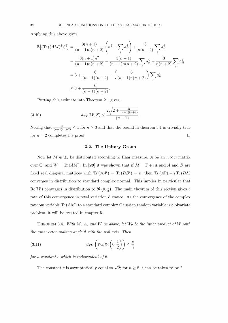
Putting this estimate into Theorem 2.1 gives:
(3.10) dTV (W,Z) ≤2√
2 + 6(n−1)(n+2)
(n− 1).
Noting that 6(n−1)(n+2) ≤ 1 for n ≥ 3 and that the bound in theorem 3.1 is trivially true
for n = 2 completes the proof.
3.2. The Unitary Group
Now let M ∈ Un be distributed according to Haar measure, A be an n × n matrix
over C, and W = Tr (AM). In [29] it was shown that if M = Γ + iΛ and A and B are
fixed real diagonal matrices with Tr (AAt) = Tr (BBt) = n, then Tr (AΓ) + iTr (BΛ)
converges in distribution to standard complex normal. This implies in particular that
Re(W ) converges in distribution to N(0, 1
2
). The main theorem of this section gives a
rate of this convergence in total variation distance. As the convergence of the complex
random variable Tr (AM) to a standard complex Gaussian random variable is a bivariate
problem, it will be treated in chapter 5.
Theorem 3.4. With M , A, and W as above, let Wθ be the inner product of W with
the unit vector making angle θ with the real axis. Then
(3.11) dTV
(Wθ,N
(0,
12
))≤ c
n
for a constant c which is independent of θ.
The constant c is asymptotically equal to√
2; for n ≥ 8 it can be taken to be 2.

3.2. THE UNITARY GROUP 39
Before beginning the proof, we give the following complex analog of Lemma 3.3 for
use here and in chapter 5.
Lemma 3.5. Let H ∈ Un be distributed according to Haar measure. Then the expected
value of a product of entries of H and their conjugates is non-zero only when there are
the same number of entries as conjugates of entries from each row and from each column.
The following are formulae for some non-zero expectations.
(i) E[|hij |2
]=
1n
,
(ii) E[|hij |4
]=
2n(n + 1)
,
(iii) E[|hij |2|hik|2
]=
1n(n + 1)
for j 6= k,
(iv) E[|hij |2|hk`|2
]=
1(n− 1)(n + 1)
for i 6= k and j 6= `,
(v) E[hijhikh`jh`k
]= − 1
(n− 1)n(n + 1),
(vi)
E[(hi1hj2 − hi2hj1)(hk1h`2 − hk2h`1)
]= −
2δi`δjk(1− δij)(n− 1)(n + 1)
+2δijδk`(1− δik)(n− 1)n(n + 1)
− 2I(i = j = k = `)n(n + 1)
,
and
(vii)
E[(hi1hj2 − hi2hj1)(hk1h`2 − hk2h`1)
]=
2δikδj`(1− δij)(n− 1)(n + 1)
− 2δijδk`(1− δik)n(n− 1)(n + 1)
+2I(i = j = k = `)
n(n + 1).
Proof. The requirement that the same number of entries as conjugates of entries
from each row and column be present is a simple consequence of the invariance properties
of Haar measure; any row or column is invariant under multiplication by a complex
number of unit modulus.
(i) Since∑
k |hik|2 = 1, this part is immediate by the invariance of Haar measure
under permuting the columns of H.
(ii) This is proved in detail in section 4.2, page 139 of [50].

40 3. LINEAR FUNCTIONS ON THE CLASSICAL MATRIX GROUPS
(iii) It suffices to assume that j = 1 and k = 2. By symmetry,
E[|hi1|2|hi2|2
]=
1n− 1
∑j 6=1
E[|hi1|2|hij |2
]=
1n− 1
E[|hi1|2
(1− |hi1|2
)]=
1n− 1
E[|hi1|2 − |hi1|4
]=
1n(n + 1)
.
(iv) This part is the same as the previous part:
E[|hi1|2|hj2|2
]=
1n− 1
∑k 6=i
E[|hi1|2|hk2|2
]=
1n− 1
E[|hi1|2
(1− |hi2|2
)]=
1(n− 1)(n + 1)
.
(v) This part makes use of the complex-orthogonality of the columns of H as well
as the invariance under permutations of the rows. It is no loss to assume that
i = j = 1 and k = ` = 2. We have
E[h11h12h21h22
]=
1n− 1
∑k 6=1
E[h11h12hk1hk2
]=
1n− 1
E[⟨
(hk1) ,(hk2
)⟩− |h11|2|h12|2
]= − 1
n− 1E[|h11|2|h12|2
]= − 1
(n− 1)n(n + 2).
(vi) This part is just putting together the previous parts. Multiplying out the
product gives
E[(hi1hj2−hi2hj1)(hk1h`2 − hk2h`1)
]= E
[hi1hk1hj2h`2 + hi2hk2hj1h`1 − hi2hk1hj1h`2 − hi1hk2hj2h`1
].

3.2. THE UNITARY GROUP 41
The first two terms integrate to zero, since H is invariant under multiplying
the first column by√−1. Thus
E[(hi1hj2 − hi2hj1)(hk1h`2 − hk2h`1)
]= E
[− hi2hk1hj1h`2 − hi1hk2hj2h`1
].
Each of these terms integrates to something non-zero if and only if either i = `
and j = k or i = j and k = `. The second term is the obtained from the
first by switching the indices 1 and 2, thus they integrate to the same thing by
spherical symmetry. It follows that
E[(hi1hj2 − hi2hj1)(hk1h`2 − hk2h`1)
]= −2E
[δi`δjk(1− δij)|hi2|2|hj1|2 + δijδk`(1− δik)hi2hk1hi1hk2
+ I(i = j = k = `)|hi1|2|hi2|2].
Part (vi) now follows from parts (iii), (iv) and (v).
(vii) This part is just like the last part. First,
E[(hi1hj2 − hi2hj1)(hk1h`2 − hk2h`1)
]= E
[hi1h`2hj2hk1 + hi2h`1hj1hk2 − hi1h`1hj2hk2 − hi2h`2hj1hk1
].
Here, the last two terms integrate to zero by symmetry. Thus
E[(hi1hj2 − hi2hj1)(hk1h`2 − hk2h`1)
]= E
[hi1h`2hj2hk1 + hi2h`1hj1hk2
].
Again, the two integrals are the same by switching the indices 1 and 2, and
each is non-zero if and only if i = k and j = ` or i = j and k = `. It follows
that
E[(hi1hj2 − hi2hj1)(hk1h`2 − hk2h`1)
]= 2E
[δikδj`(1− δij)|hi1|2|hj2|2 + δijδk`(1− δik)hi1hk2hi2hk1
+ I(i = j = k = `)|hi1|2|hi2|2];
the formula of part (vii) follows from parts (iv), (v) and (ii).

42 3. LINEAR FUNCTIONS ON THE CLASSICAL MATRIX GROUPS
Proof of Theorem 3.4. To prove the theorem, first note that it suffices to con-
sider the case θ = 0, that is, to prove that
dTV
(Re(W ),N
(0,
12
))≤ c
n;
the theorem then follows as stated since the distribution of W is invariant under multi-
plication by any complex number of unit modulus. By the singular value decomposition
(see, e.g., [14], page 6), there is an n × n diagonal matrix S with non-negative entries
such that A = USV for two unitary matrices U and V . Then Tr (AM) = Tr (USV M) =
Tr (SV MU) and V MU has the same distribution as M by the translation invariance of
Haar measure. It follows that A can be assumed to be diagonal with non-negative real
entries.
The proof is almost identical to the orthogonal case. Let H ∈ Un be a random
unitary matrix, independent of M , and let Mε = HAεH∗M , where
Aε =
√1− ε2 ε
−ε√
1− ε2 0
1
0. . .
1
.
Let Wε = W (Mε).
Let I2 be the 2 × 2 identity matrix, K the n × 2 matrix made from the first two
columns of H, and let
C2 =
0 1
−1 0
.
Then
Wε −W = Tr((
−ε2
2+ O(ε4)
)AKK∗M + εAKC2K
∗M
)= ε
[(− ε
2+ O(ε3)
)Tr (AKK∗M) + Tr (AKC2K
∗M)].(3.12)
3.2. THE UNITARY GROUP 43
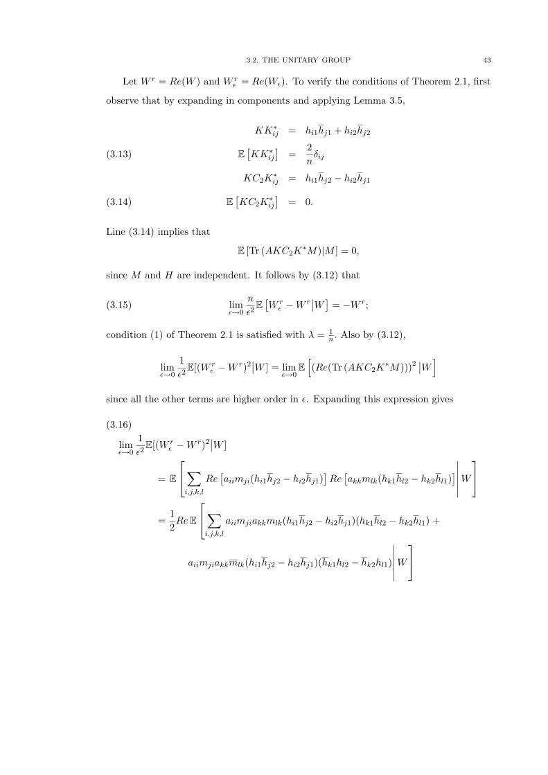
Let W r = Re(W ) and W rε = Re(Wε). To verify the conditions of Theorem 2.1, first
observe that by expanding in components and applying Lemma 3.5,
KK∗ij = hi1hj1 + hi2hj2
E[KK∗
ij
]=
2n
δij(3.13)
KC2K∗ij = hi1hj2 − hi2hj1
E[KC2K
∗ij
]= 0.(3.14)
Line (3.14) implies that
E [Tr (AKC2K∗M)|M ] = 0,
since M and H are independent. It follows by (3.12) that
(3.15) limε→0
n
ε2E[W r
ε −W r∣∣W ]
= −W r;
condition (1) of Theorem 2.1 is satisfied with λ = 1n . Also by (3.12),
limε→0
1ε2
E[(W rε −W r)2
∣∣W ] = limε→0
E[(Re(Tr (AKC2K
∗M)))2∣∣W]
since all the other terms are higher order in ε. Expanding this expression gives
limε→0
1ε2
E[(W rε −W r)2
∣∣W ]
= E
∑i,j,k,l
Re[aiimji(hi1hj2 − hi2hj1)
]Re[akkmlk(hk1hl2 − hk2hl1)
]∣∣∣∣∣∣W
=12Re E
∑i,j,k,l
aiimjiakkmlk(hi1hj2 − hi2hj1)(hk1hl2 − hk2hl1) +
aiimjiakkmlk(hi1hj2 − hi2hj1)(hk1hl2 − hk2hl1)
∣∣∣∣∣∣W
(3.16)

44 3. LINEAR FUNCTIONS ON THE CLASSICAL MATRIX GROUPS
Let∑′
i,j
stand for summing over all pairs (i, j) where i and j are distinct. Applying
parts (vi) and (vii) of Lemma 3.5 now gives
limε→0
n
2ε2E[(
W rε −W r
)2∣∣W ]=
n
2(n− 1)(n + 1)Re E
∑i,j,k,`
aiimjiakkm`k
(−δi`δjk(1− δij) +
1n
δijδk`(1− δik)
−(
n− 1n
)I(i = j = k = `)
)+∑
i,j,k,`
aiimjiakkm`k
(δikδj`(1− δij)−
1n
δijδk`(1− δik)
+(
n− 1n
)I(i = j = k = l)
)∣∣∣∣∣W]
=n
2(n− 1)(n + 1)Re E
−∑′
i,j
aiiajjmijmji +1n
∑′
i,k
aiiakkmiimkk
−(
n− 1n
)∑i
a2iim
2ii +
∑′
i,j
a2ii|mji|2
− 1n
∑′
i,k
aiiakkmiimkk +n− 1
n
∑i
a2ii|mii|2
∣∣∣∣∣W]
=n
2(n− 1)(n + 1)Re E
[−
(Tr ((AM)2)−
∑i
(AM)2ii
)+
1n
(W 2 −
∑i
(AM)2ii
)
−(
n− 1n
)∑i
(AM)2ii +∑
i
a2ii(1− |mii|2)
− 1n
(|W |2 −
∑i
a2ii|mii|2
)+
n− 1n
∑i
a2ii|mii|2
∣∣∣∣∣W]
=12
+1
2(n− 1)(n + 1)
+n
2(n− 1)(n + 1)Re E
[−Tr ((AM)2) +
W 2 − |W |2
n
∣∣∣∣W].
Condition (2) of Theorem 2.1 is thus satisfied with
nE =1
2(n− 1)(n + 1)+
n
2(n− 1)(n + 1)Re E
[−Tr ((AM)2) +
W 2 − |W |2
n
∣∣∣∣W],
(3.17)
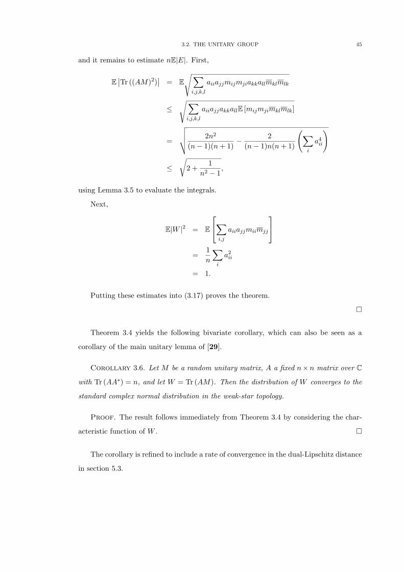
3.2. THE UNITARY GROUP 45
and it remains to estimate nE|E|. First,
E∣∣Tr ((AM)2)
∣∣ = E√∑
i,j,k,l
aiiajjmijmjiakkallmklmlk
≤√∑
i,j,k,l
aiiajjakkallE [mijmjimklmlk]
=
√√√√ 2n2
(n− 1)(n + 1)− 2
(n− 1)n(n + 1)
(∑i
a4ii
)
≤√
2 +1
n2 − 1,
using Lemma 3.5 to evaluate the integrals.
Next,
E|W |2 = E
∑i,j
aiiajjmiimjj
=
1n
∑i
a2ii
= 1.
Putting these estimates into (3.17) proves the theorem.
Theorem 3.4 yields the following bivariate corollary, which can also be seen as a
corollary of the main unitary lemma of [29].
Corollary 3.6. Let M be a random unitary matrix, A a fixed n×n matrix over C
with Tr (AA∗) = n, and let W = Tr (AM). Then the distribution of W converges to the
standard complex normal distribution in the weak-star topology.
Proof. The result follows immediately from Theorem 3.4 by considering the char-
acteristic function of W .
The corollary is refined to include a rate of convergence in the dual-Lipschitz distance
in section 5.3.

46 3. LINEAR FUNCTIONS ON THE CLASSICAL MATRIX GROUPS

CHAPTER 4
Eigenfunctions of the Laplacian
The results of this chapter are an abstraction of the results of section 2.1 and chapter
3. In those cases, a specific class of functions (linear) were considered on three specific
manifolds – the sphere, the orthogonal group, and the unitary group. The exchange-
able pair in each case was a small random rotation. Here, this approach is generalized
to a large class of Riemannian manifolds, with the linear functions being replaced by
eigenfunctions of the Laplacian.
Eigenvalues and eigenfunctions of the Laplacian ∆g on a Riemannian manifold (M, g)
have appeared as important and interesting objects in several branches of analysis. The
spectrum of the Laplacian is a central object of study in spectral geometry, which is
concerned with relationships between the spectrum of ∆g and the geometry of M . In
particular, spectral geometry deals with inverse problems such as Mark Kac’s [57] famous
question, “Can you hear the shape of a drum?” More specifically, how much information
can one recover about the geometry of a manifold from knowledge of the spectrum of
its Laplacian? Weyl [82] showed that you can determine the volume of the manifold: if
N(λ) denotes the number of eigenvalues less than λ, he showed that
limλ→∞
N(λ)λ
=vol(M)
2π.
Milnor [65] showed that not all information about the manifold could be recovered. He
found two Riemannian flat tori of dimension 16 which were not isometric, yet whose
Laplacians had the same sequence of eigenvalues.
Eigenvalues and eigenfunctions of the Laplacian are also of central interest in quan-
tum chaos. An important open question in the field is whether the quantum unique
ergodicity conjecture of Rudnick and Sarnak [73] holds. The conjecture is the following.
47

48 4. EIGENFUNCTIONS OF THE LAPLACIAN
Conjecture 4.1 (Rudnick-Sarnak). Let M be a compact hyperbolic surface, and let
φk∞k=1 be a sequence of linearly independent eigenfunctions of the Laplacian ∆g on M ,
normalized to have L2-norm one. Then the probability measures µk defined by
µk(A) =∫
A|φk(x)|2 dvol(x)
converge to the measure vol in the weak-star topology.
Snirel′man [77], Colin de Verdiere [28], and Zelditch [83] have shown that the con-
jecture is true up to the removal of a subsequence of density zero, on manifolds on which
the geodesic flow is ergodic. The conjecture above is consistent with the ‘random wave
model’ of eigenstates (see [13]), which conjectures that individual eigenfunctions behave
like random waves. See Sarnak [74] for an introduction to this area of study. In partic-
ular, it is discussed in [74] that a consequence of the random wave model would be that
high eigenfunctions would be approximately normally distributed. In connection with
this conjecture, Hejhal and various coauthors (see, e.g., [49]) and Aurich and Steiner
[3] have provided numerical evidence indicating that on certain hyperbolic manifolds,
the distributions of eigenfunctions become close to Gaussian as the eigenvalue tends
to infinity. Theorem 4.3 below suggests a possible approach to rigorous results in this
direction.
In this chapter we will freely use standard facts and notations of Riemannian geome-
try. For an introduction to the ideas used here, see the book [24] of Chavel, particularly
chapters 1 and 3.
Let (M, g) be an n-dimensional Riemannian manifold. Integration with respect to
the normalized volume measure is denoted dvol, thus∫M 1dvol = 1. For a linearly inde-
pendent set of vector fields
∂∂xi
n
i=1, define
(G(x))ij = gij(x) =⟨
∂
∂xi
∣∣∣∣x
,∂
∂xj
∣∣∣∣x
⟩, g(x) = det(G(x)), gij(x) = (G−1(x))ij .
Define the gradient ∇f of f : M → R and the Laplacian ∆gf of f by
∇f(x) =∑j,k
∂f
∂xjgjk ∂
∂xk, ∆gf(x) =
1√
g
∑j,k
∂
∂xj
(√
ggjk ∂f
∂xk
).

4. EIGENFUNCTIONS OF THE LAPLACIAN 49
Let Φt(x, v) denote the geodesic flow on the tangent bundle TM and let π : TM →
M be the projection map of a tangent vector onto its base point. Recall that the
manifold is said to have ‘bounded geometry’ if there is a non-trivial lower bound on the
injectivity radius of the exponential map. We call a Riemannian manifold M locally
weakly symmetric if M has bounded geometry, and there is an ε with expx(t, v) injective
on the unit tangent bundle SM for t ∈ (−ε, ε), such that the volume measure on M is
invariant under the substitution
π Φt(x, v) → π(−Φt(x, v))
for t ∈ (−ε, ε). In particular, a compact locally symmetric space is weakly locally sym-
metric. The class of manifolds considered here is thus quite broad and includes Lie
groups, quotients of Lie groups, flat tori and tori of genus at least two with hyperbolic
geometry.
In what follows, some basic facts about the Laplacian on a Riemannian manifold are
needed. Chavel’s book [23] is a good source of background; in particular, the following
theorem is Theorem 1 of section 1.3 (page 8).
Theorem 4.2 (see [23]). Let M be a compact, connected Riemannian manifold with-
out boundary. The set of real numbers λ for which there exists a nontrivial solution
ϕ ∈ C2(M) to
∆ϕ + λϕ = 0
consists of a sequence
0 ≤ λ1 < λ2 · · · ↑ +∞
and each associated eigenspace is finite dimensional. Eigenspaces belonging to distinct
eigenvalues are orthogonal in L2(M), and L2(M) is the direct sum of all the eigenspaces.
Furthermore, each eigenfunction is C∞ on M .
The following theorem is the main result of this section.
Theorem 4.3. Let M be a finite-volume locally weakly symmetric space (without
boundary), and f an eigenfunction for the Laplacian on M with eigenvalue λ 6= 0,

50 4. EIGENFUNCTIONS OF THE LAPLACIAN
normalized so that∫M f2dvol = 1. Let X be a random (i.e., distributed according to
normalized volume measure) point of M . Then
dTV (f(X), Z) ≤ 1|λ|
√Var(‖∇f(X)‖2
),
where Z is a standard Gaussian random variable on R.
Proof. Start by constructing a family of exchangeable pairs of points in M parametrized
by ε. Let X be a random point of M and let ε > 0 be smaller than the injectivity radius
of the exponential map at X. Since M has bounded geometry, there is a range of ε
small enough to work at every point. Now, choose a unit vector V ∈ TXM at random,
independent of X, and define
Xε = expX(εV ).
The fact that M is a locally weakly symmetric space implies that the pair (X, Xε) is
exchangeable. To see this, we show that∫M×M
g(x, xε)dµ =∫
M×Mg(xε, x)dµ
for all integrable g : M ×M → R, where µ is the measure defined by the construction of
the pair (X, Xε).
Let L denote the normalized Liouville measure on SM , which is locally the product
of the normalized volume measure on M and normalized Lebesgue measure on the unit
spheres of TxM . The measure L also has the property that it is invariant under the
geodesic flow Φt(x, v). See [24], section 5.1 for a construction of L and proofs of its key
properties. By construction of the measure µ,∫M×M
g(x, xε)dµ =∫
SMg(x, π Φε(x, v))dL(x, v)
=∫
SMg(π Φ−ε(y, η), y)dL(y, η)
by the substitution (y, η) = Φε(x, v), since Liouville measure is invariant under the
geodesic flow. Now,
Φ−ε(y, η) = −Φε(y,−η),

4. EIGENFUNCTIONS OF THE LAPLACIAN 51
as both correspond to going backwards on the same geodesic. It follows that∫SM
g(x, xε)dL(x, v) =∫
SMg(π(−Φε(y,−η)), y)dL(y, η)
=∫
SMg(π(−Φε(y, η)), y)dL(y, η)
=∫
SMg(π(Φε(y, η)), y)dL(y, η)
=∫
SMg(yε, y)dµ,
where the second line follows from the substitution −η → η, under which Lebesgue
measure on the tangent space is invariant, and the third line follows by the symmetry
assumption on M . Thus the pair (X, Xε) is exchangeable as required.
Now, let f be an eigenfunction of the Laplacian on M with eigenvalue λ < 0 and
‖f‖2 = 1. Recall that the eigenspaces of the Laplacian are orthogonal and that a constant
function on M is an eigenfunction with eigenvalue 0, thus∫M fdµ = 0. A consequence
of Stokes’ theorem is that ∫M
f∆fdvol = −∫
M‖∇f‖2dvol.
Since f is an eigenfunction with eigenvalue λ and ‖f‖2 = 1, this means that
1|λ|
∫M‖∇f‖2dvol = 1.
For notational convenience, let W = f(X) and Wε = f(Xε). Since (X, Xε) is ex-
changeable, (W,Wε) is an exchangeable pair as well.
In order to verify the conditions of Theorem 2.1, first let γ : [0, 1] → M be a constant-
speed geodesic such that γ(0) = X, γ(1) = Xε, and γ′(0) = εV . Then applying Taylor’s
theorem on R to the function f γ yields
f(Xε)− f(X) = ε · d(f γ)dt
∣∣∣∣t=0
+ ε2 · d2(f γ)dt2
∣∣∣∣t=0
+ O(ε3)
= ε · dXf(V ) + ε2 · d2(f γ)dt2
∣∣∣∣t=0
+ O(ε3),
(4.1)
where the coefficient implicit in the O(ε3) depends on f and γ and dxf denotes the
differential of f at x. Recall that dxf(v) = 〈∇f(x), v〉 for v ∈ TxM and the gradient

52 4. EIGENFUNCTIONS OF THE LAPLACIAN
∇f(x) defined as above. Now, for X fixed, V is distributed according to normalized
Lebesgue measure on SXM and dXf is a linear functional on TXM . It follows that
E[dXf(V )
∣∣X] = E[dXf(−V )
∣∣X] = −E[dXf(V )
∣∣X] ,so
E[dXf(V )
∣∣X] = 0.
This implies that
limε→0
1ε2
E[f(Xε)− f(X)
∣∣X]exists and is finite.
Claim 4.4.
limε→0
1ε2
E[f(Xε)− f(X)
∣∣X] =12n
∆gf(X) =λ
2nf(X).
Proof. Let SεX denote the geodesic sphere of radius ε in M centered at X, and
let BεX be the corresponding geodesic ball. Let A be the area form on Sε
X ; that is, dA
denotes integration over SεX with respect to the volume measure given by the Riemannian
structure. Then
limε→0
1ε2
E[f(Xε)− f(X)
∣∣X]= lim
ε→0
1ε2A(Sε
X)
∫Sε
X
[f(Xε)− f(X)
]dA(v)
= limε→0
1εA(Sε
X)
∫Sε
X
1ε
∫ 1
0
⟨∇f, γ′(t)
⟩γ(t)
dtdA(v)
= limε→0
1εA(Sε
X)
∫Sε
X
1ε
∫ 1
0
[ε 〈v,∇f〉X + ε2t 〈v,∇v(∇f)〉X
+⟨γ′(t),∇f
⟩γ(t)
− 〈εv,∇f + t∇εv(∇f)〉X]dtdA(v),
(4.2)
by the fundamental theorem of calculus. (Recall that ∇v denotes the covariant derivative
in the direction v.)
Now, ∫Sε
X
〈v,∇f〉X dA(v) = 0

4. EIGENFUNCTIONS OF THE LAPLACIAN 53
by symmetry as discussed above (the area form on SεX pulls back to uniform measure on
the sphere in the tangent space), so the first term of (4.2) is zero.
For the last term, note that 〈γ′(t),∇f〉γ(t) − 〈εv,∇f + t∇εv(∇f)〉X = 0 for t = 0.
The first derivative with respect to t of this expression is
⟨γ′(t),∇γ′(t)(∇f)
⟩γ(t)
− 〈εv,∇εv(∇f)〉X
(which is also zero at t = 0) and the second derivative is
⟨γ′(t),∇γ′(t)(∇γ′(t)(∇f))
⟩γ(t)
,
using the fact that ∇γ′(t)(γ′(t)) = 0, since γ is a geodesic. This last expression is O(ε3),
since ‖γ′(t)‖ = ε for each t, and f is smooth, so taking the limit gives
limε→0
1ε2
E[f(Xε)− f(X)
∣∣X] = limε→0
12A(Sε
X)
∫Sε
X
〈v,∇v(∇f)〉X dA
=1
2σ(Sn−1)
∫Sn−1⊆TXM
〈v,∇v(∇f)〉 dσ(v),(4.3)
where σ is uniform measure on the sphere. This is now an integral over a Euclidean
sphere. Choose an orthonormal basis
∂∂xi
∣∣∣X
of TXM which extends to Riemannian
coordinates in a neighborhood of X. Then at X,
gij = δij , gij = δij , g = 1,
thus
∆gf(X) =∑
i
∂2f
∂x2i
.
Expressing the integrand in these coordinates gives:
limε→0
1ε2
E[f(Xε)− f(X)
∣∣X] =1
2σ(Sn−1)
∫Sn−1⊆TXM
∑i,j
vivj
⟨∂
∂xi,∇ ∂
∂xj
(∇f)⟩
dσ(v)
=12
∑i
1n
∂2f
∂x2i
=12n
∆gf(X)
=λ
2nf(X),

54 4. EIGENFUNCTIONS OF THE LAPLACIAN
since E[vivj
]= 1
nδij for v uniform on the sphere with vi the coordinates of v in an
orthonormal basis.
Consider next
limε→0
1ε2
E[(Wε −W )2
∣∣X].By the expansion (4.1),
E[(Wε −W )2
∣∣X] = E[(f(Xε)− f(X))2
∣∣X]= ε2E
[(dxf(v))2
∣∣X]+ O(ε3).
In the coordinates introduced above,
∇f(X) =∑
i
∂f
∂xi
∂
∂xi,
thus
[dxf(v)]2 = [〈∇f, v〉]2
=n∑
i=1
(∂f
∂xi
)2
v2i +
∑i6=j
∂f
∂xi
∂f
∂xjvivj .
Making use again of the independence of v and X and the fact that E[vivj ] = 1nδij yields
limε→0
1ε2
E[(dxf(v))2
∣∣X] =1n‖∇f‖2 = −λ
n+
1n
[‖∇f‖2 + λ
],
thus condition (2) is satisfied with
E =2λ
[‖∇f‖2 + λ
].
Finally, (4.1) gives immediately that
limε→0
1ε2
E[|Wε −W |3
∣∣W ]= 0.
Recall that E‖∇f‖2 = −λ; the proof is completed by applying the Cauchy-Schwarz
inequality to E|E|.

4.1. EXAMPLE: SECOND ORDER SPHERICAL HARMONICS 55
4.1. Example: Second order spherical harmonics
In section 2.1, linear functions of a random point on the sphere were shown to be
approximately normally distributed. The following theorem is a non-linear example of
an application of Theorem 4.3, treating quadratic functions of the form∑
i,j aijxixj of
a random point on the sphere. These are eigenfunctions of the Laplacian on the sphere
with eigenvalue λ = −2n provided that Tr (A) =∑
i aii = 0. Some examples and
remarks illustrating the theorem appear after the proof.
Theorem 4.5. Let g(x) =∑
i,j aijxixj , where A = (aij)ni,j=1 is a symmetric matrix
with Tr (A) = 0. Let f = Cg, where C is chosen such that ‖f‖2 = 1 when f is considered
as a function on Sn−1. Let W = f(X), where X is a random point on Sn−1. If d is the
vector in Rn whose entries are the eigenvalues of A, then
dTV (W,Z) ≤√
5(‖d‖4
‖d‖2
)2
,
where ‖d‖p = (∑
i |di|p)1/p .
Proof. To apply Theorem 4.3, it is first necessary to show that f is indeed an
eigenfunction of the Laplacian on Sn−1 and to identify its eigenvalue. It is discussed
in section 9.5 of [81] that the eigenfunctions of the spherical Laplacian are exactly the
restrictions of homogeneous harmonic polynomials on Rn to the sphere, and that such
polynomials of degree l have eigenvalue −l(l + n− 2). It is trivial to verify that since A
is traceless, g is harmonic on Rn and thus is an eigenfunction with eigenvalue λ = −2n.
Next, note that g(x) = 〈x,Ax〉 , and A is a symmetric matrix, so A = U∗DU for a
diagonal matrix D and an orthogonal matrix U . Thus
g(x) = 〈x,U∗DUx〉 = 〈Ux, DUx〉 .
Since the uniform distribution on the sphere is invariant under the action of the orthog-
onal group, this observation means that it suffices to prove the theorem in the case that
A = diag(a1, . . . , an).

56 4. EIGENFUNCTIONS OF THE LAPLACIAN
By Theorem 4.3,
dTV (W,Z) ≤ 1|λ|
√V ar
(‖∇f‖2
),
and the main task of the proof is to estimate the right-hand side. A consequence of
Stokes’ theorem is that ∫Sn−1
‖∇g‖2dσ = |λ|∫
Sn−1
g2dσ,
so one can calculate E‖∇g‖2 in order to determine C. The spherical gradient ∇g is
just the projection onto the hyperplane orthogonal to the radial direction of the usual
gradient. Letting∑′
stand for summing over distinct indexes,
E‖∇Sn−1g(x)‖2 = E‖∇Rng(x)‖2 − E (x · ∇Rng(x))2
= E
[n∑
i=1
4a2i x
2i
]− 4E
n∑i=1
a2i x
4i +
∑′
i,j
aiajx2i x
2j
=
4n
n∑i=1
a2i −
4n(n + 2)
3∑
i
a2i +
∑′
i,j
aiaj
=
4n
n∑i=1
a2i −
4n(n + 2)
2∑
i
a2i +
(n∑
i=1
ai
)2
=4
n + 2
n∑i=1
a2i ,
where Lemma 1.6 (after renormalization) has been used to get the third line, and the
fact that Tr (A) = 0 is used to get the last line. From this computation it follows that
the constant C in the statement of the theorem should be taken to be√
n(n+2)2‖a‖22
, where
a = (ai)ni=1.
Now,
E‖∇Sn−1g‖4 ≤ E‖∇Rng‖4,
since ∇Sn−1g is a projection of ∇Rng.
E‖∇Rng‖4 = 16 E
n∑i=1
a4i x
4i +
∑′
i,j
a2i a
2jx
2i x
2j
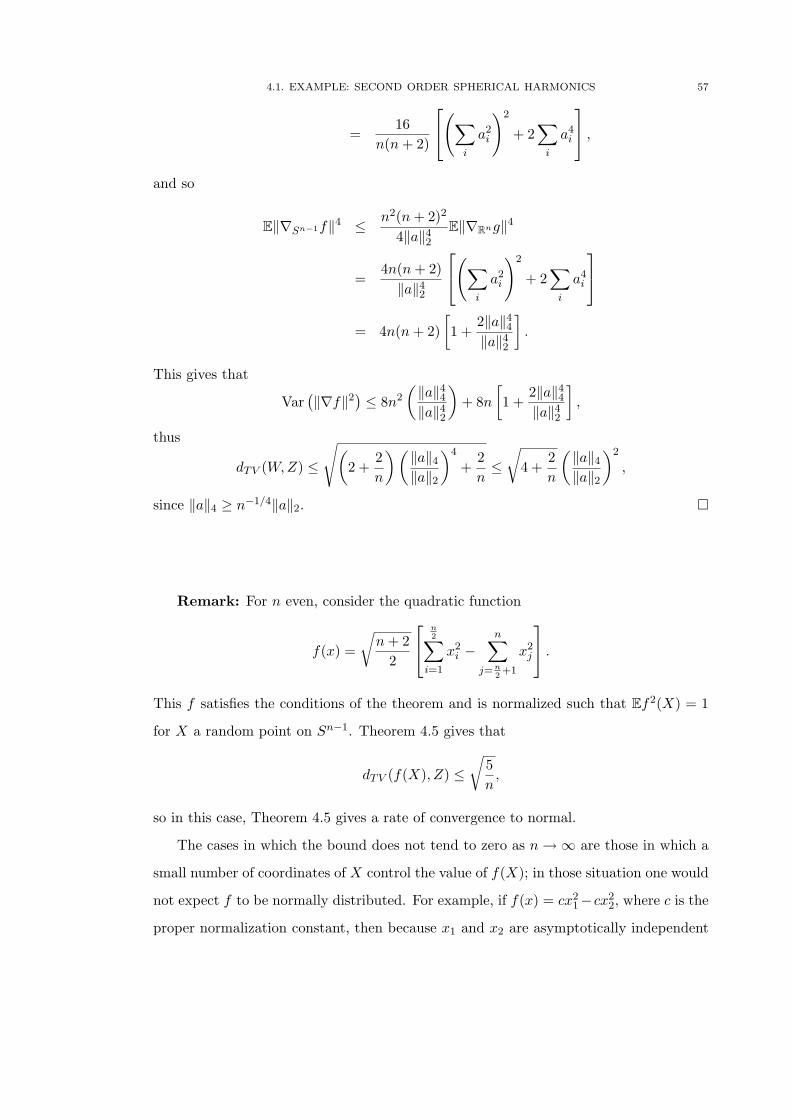
4.1. EXAMPLE: SECOND ORDER SPHERICAL HARMONICS 57
=16
n(n + 2)
(∑i
a2i
)2
+ 2∑
i
a4i
,
and so
E‖∇Sn−1f‖4 ≤ n2(n + 2)2
4‖a‖42
E‖∇Rng‖4
=4n(n + 2)‖a‖4
2
(∑i
a2i
)2
+ 2∑
i
a4i
= 4n(n + 2)
[1 +
2‖a‖44
‖a‖42
].
This gives that
Var(‖∇f‖2
)≤ 8n2
(‖a‖4
4
‖a‖42
)+ 8n
[1 +
2‖a‖44
‖a‖42
],
thus
dTV (W,Z) ≤
√(2 +
2n
)(‖a‖4
‖a‖2
)4
+2n≤√
4 +2n
(‖a‖4
‖a‖2
)2
,
since ‖a‖4 ≥ n−1/4‖a‖2.
Remark: For n even, consider the quadratic function
f(x) =
√n + 2
2
n2∑
i=1
x2i −
n∑j=n
2+1
x2j
.
This f satisfies the conditions of the theorem and is normalized such that Ef2(X) = 1
for X a random point on Sn−1. Theorem 4.5 gives that
dTV (f(X), Z) ≤√
5n
,
so in this case, Theorem 4.5 gives a rate of convergence to normal.
The cases in which the bound does not tend to zero as n →∞ are those in which a
small number of coordinates of X control the value of f(X); in those situation one would
not expect f to be normally distributed. For example, if f(x) = cx21−cx2
2, where c is the
proper normalization constant, then because x1 and x2 are asymptotically independent

58 4. EIGENFUNCTIONS OF THE LAPLACIAN
Gaussian random variables (see section 5.2), f is asymptotically distributed as c(Z21−Z2
2 )
for independent Gaussians Z1 and Z2.

CHAPTER 5
Multivariate normal approximation
5.1. A multivariate abstract approximation theorem
This section contains the statement and proof of a multivariate analog to Theorem
2.1; the results of this section are joint work with Sourav Chatterjee.
There has been some previous work in using Stein’s method for multivariate normal
approximation. Rinott and Rotar used a ‘two level’ dependency graph approach to prove
central limit theorems for dependent random vectors, which they applied to studying
statistics on nearest neighbor random graphs. Their approach yields bounds on
∣∣Eh(W )− Eh(Z)∣∣
for Z a multivariate Gaussian random vector, W the random vector being studied, and
h in a class H of (not necessarily smooth) functions. They restrict attention to classes
of functions H with the following properties. For h : Rn → R, set
h+ε = suph(x + y) : |y| ≤ ε, h−ε = infh(x + y) : |y| ≤ ε,
h(x; ε) = h+ε (x)− h−ε (x).
Then it is required of H that
(i) If h ∈ H, ‖h‖∞ ≤ 1.
(ii) If h ∈ H, then h+ε ∈ H and h−ε ∈ H for any ε > 0.
(iii) For any n× n matrix A and vector b ∈ Rn, if h ∈ H then h(Ax + b) ∈ H.
(iv) For all ε > 0,
supEh(Z; ε) : h ∈ H < aε,
where Z ∼ N(0, 1) and a is a constant depending only on H and n.
The constant a is sometimes called the isoperimetric constant of H.
59

60 5. MULTIVARIATE NORMAL APPROXIMATION
The class H can for example be taken to be the indicator functions of convex sets.
However, the restrictions on H are enough that their approach does not yield a bound
in total variation distance.
Goldstein and Rinott [46] have also developed a technique for multivariate normal
approximation using Stein’s method and size-bias coupling, where the dependence in the
problem need not be local. They apply their techniques to statistics of random graphs.
The notion of distance used is bounding
Eh(W )− Eh(Z)
over a class of smooth functions h.
More recently, Goldstein and Reinert [45] have developed a version of multivariate
normal approximation using Stein’s method together with zero-bias coupling, with ap-
plications to simple random sampling. The also consider a notion of distance which
compares expectations of smooth functions with respect to the random variable in ques-
tion and the normal distribution.
In the univariate case, there are problems which are most easily treated via the
method of exchangeable pairs than other approaches to Stein’s method, e.g., when the
random variable under study depends on an underlying reversible Markov chain. See
in particular the analysis of the antivoter chain in [71] and the examples in [33]. This
partly motivated the development of a multivariate version of the method of exchangeable
pairs in [22]. Another motivation for this development is the fact that the extension of
Stein’s method to situations with continuous symmetries given in chapter 2 seems very
well suited to work with the method of exchangeable pairs. This is still the case in a
multivariate context; see Theorem 5.3 below.
The following lemma gives a second-order characterizing operator for the Gaussian
distribution on Rk. For f ∈ C1(Rk), define the gradient of f by∇f(x) = ( ∂f∂x1
(x), . . . , ∂f∂xk
(x))t.
Define the Laplacian of f by ∆f(x) =∑k
i=1∂2f∂x2
i(x).
Lemma 5.1. Let Z ∈ Rk be a random vector with Zi i.i.d. standard Gaussians.

5.1. A MULTIVARIATE ABSTRACT APPROXIMATION THEOREM 61
(i) If f : Rk → R is two times continuously differentiable and compactly supported,
then
E[∆f(Z)− Z · ∇f(Z)
]= 0.
(ii) If Y ∈ Rk is a random vector such that
E[∆f(Y )− Y · ∇f(Y )
]= 0
for every f ∈ C2(Rk), then L(Y ) = L(Z).
(iii) If g ∈ C∞o (Rk), then the function
Uog(x) :=∫ 1
0
12t
[Eg(
√tx +
√1− tZ)− Eg(Z)
]dt
is a solution to the differential equation
(5.1) ∆h(x)− x · ∇h(x) = g(x)− Eg(Z).
Proof. Part (i) is just integration by parts.
For part (iii), first note that since g is Lipschitz, if t ∈(0, 1
2
)and L is the Lipschitz
constant of g,∣∣∣∣ 12t
[Eg(
√tx +
√1− tZ)− Eg(Z)
]∣∣∣∣ ≤ L
2tE∣∣∣√tx + (
√1− t− 1)Z
∣∣∣≤ L
2t
[√t|x|+ t√
2
√k
],
which is integrable on(0, 1
2
), and the integrand is bounded on
(12 , 1), so the integral
exists by the dominated convergence theorem.
To show that it is indeed a solution to the differential equation (5.1), let
Zt =√
tx +√
1− tZ
and observe that
g(x)− Eg(Z) =∫ 1
0
d
dtEg(Zt)dt
=∫ 1
0
12√
tE(x · ∇g(Zt))dt−
∫ 1
0
12√
1− tE(Z · ∇g(Zt))dt

62 5. MULTIVARIATE NORMAL APPROXIMATION
=∫ 1
0
12√
tE(x · ∇g(Zt))dt−
∫ 1
0
12
E(∆g(Zt))dt
by integration by parts. Noting that
∆(Uog)(x) =∫ 1
0
12
E(∇g(Zt))dt
and
x · ∇(Uog)(x) =∫ 1
0
12√
tE(x · ∇g(Zt))dt
completes part (iii).
Finally, if
E[∆f(Y )− Y · ∇f(Y )
]= 0
for every f ∈ C2(Rk), then for g ∈ C∞o given,
Eg(Y )− Eg(Z) = E[∆(Uog)(Y )− Y · ∇(Uog)(Y )
]= 0,
and so L(Y ) = L(Z) since C∞o is dense in the class of bounded continuous functions
vanishing at infinity, with respect to ‖ · ‖∞.
The next lemma gives various useful bounds on Uog and its derivatives in terms of
g and its derivatives. Below, |∇g| is the length of the gradient vector ∇g, thus ‖|∇g|‖∞
denotes the supremum of |∇g(x)| over x ∈ Rk.
Lemma 5.2. For g ∈ C3o (Rk), Uog satisfies the following bounds:
(i) For all 1 ≤ i ≤ k, ∥∥∥∥∂(Uog)∂xi
∥∥∥∥∞≤ 1√
2‖g‖∞.
(ii) For 1 ≤ i, j ≤ k, ∥∥∥∥∂2(Uog)∂xi∂xj
∥∥∥∥∞≤∥∥∥∥ ∂g
∂xj
∥∥∥∥∞
.
(iii) If H is the Hessian matrix of Uog, then
‖H‖H.S. =√
Tr (HHt) ≤√
k‖|∇g|2‖∞
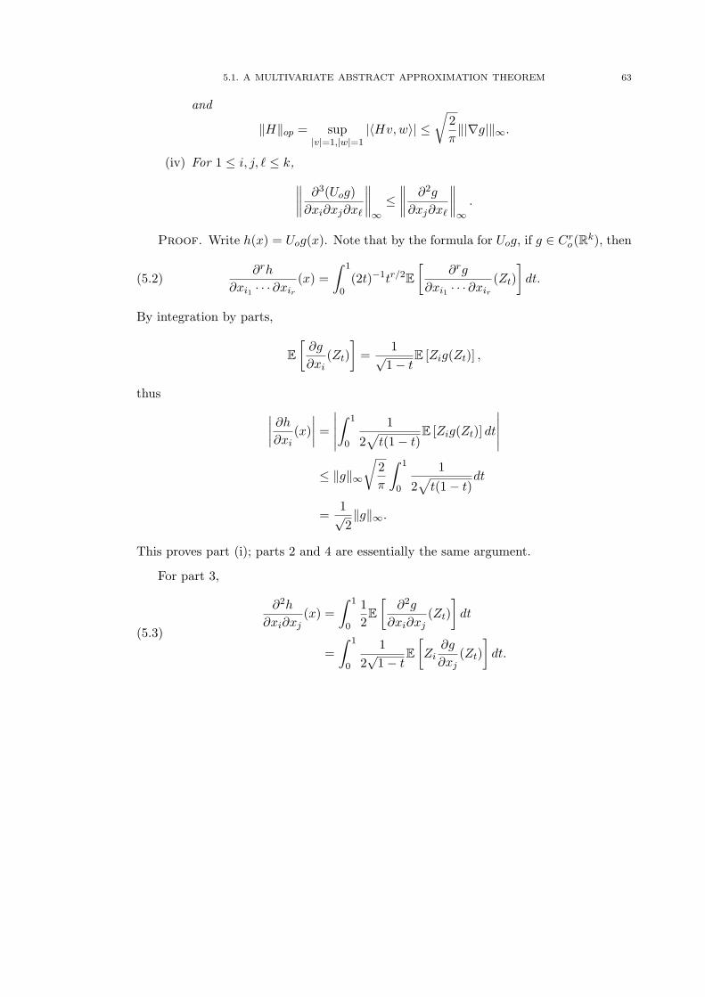
5.1. A MULTIVARIATE ABSTRACT APPROXIMATION THEOREM 63
and
‖H‖op = sup|v|=1,|w|=1
|〈Hv, w〉| ≤√
2π‖|∇g|‖∞.
(iv) For 1 ≤ i, j, ` ≤ k,∥∥∥∥ ∂3(Uog)∂xi∂xj∂x`
∥∥∥∥∞≤∥∥∥∥ ∂2g
∂xj∂x`
∥∥∥∥∞
.
Proof. Write h(x) = Uog(x). Note that by the formula for Uog, if g ∈ Cro(Rk), then
(5.2)∂rh
∂xi1 · · · ∂xir
(x) =∫ 1
0(2t)−1tr/2E
[∂rg
∂xi1 · · · ∂xir
(Zt)]
dt.
By integration by parts,
E[
∂g
∂xi(Zt)
]=
1√1− t
E [Zig(Zt)] ,
thus ∣∣∣∣ ∂h
∂xi(x)∣∣∣∣ =
∣∣∣∣∣∫ 1
0
12√
t(1− t)E [Zig(Zt)] dt
∣∣∣∣∣≤ ‖g‖∞
√2π
∫ 1
0
12√
t(1− t)dt
=1√2‖g‖∞.
This proves part (i); parts 2 and 4 are essentially the same argument.
For part 3,
∂2h
∂xi∂xj(x) =
∫ 1
0
12
E[
∂2g
∂xi∂xj(Zt)
]dt
=∫ 1
0
12√
1− tE[Zi
∂g
∂xj(Zt)
]dt.
(5.3)

64 5. MULTIVARIATE NORMAL APPROXIMATION
Summing in k gives
k∑j=1
(∂2h
∂xi∂xj(x))2
=k∑
j=1
(∫ 1
0
12√
1− tE[Zi
∂g
∂xj(Zt)
]dt
)2
≤∫ 1
0
12√
1− tE
Z2i
k∑j=1
(∂g
∂xj(Zt)
)2 dt
≤ ‖|∇g|2‖∞,
where the second line follows by two applications of Jensen’s inequality, first considering
the function E[Zi
∂g∂xj
(Zt)]
being integrated with respect to 12√
1−tdt on (0, 1), then to
the expression(E[Zi
∂g∂xj
(Zt)])2
. Summing in i now gives that ‖H(x)‖2H.S. ≤ k‖|∇g|2‖∞
for all x.
The bound on ‖H‖op is proved similarly. Making use of equation (5.3),
|〈Hv, w〉| =
∣∣∣∣∣∣∫ 1
0
12√
1− tE
( k∑i=1
viZi
) k∑j=1
wj∂g
∂xj(Zt)
dt
∣∣∣∣∣∣=∣∣∣∣∫ 1
0
12√
1− tE [〈v, Z〉 〈w,∇g(Zt)〉] dt
∣∣∣∣≤ ‖|∇g|‖∞
∫ 1
0
12√
1− tE |〈v, Z〉| dt
≤ ‖|∇g|‖∞
√2π
,
since 〈v, Z〉 is a standard Gaussian random variable.
The following is a multivariate analog of Theorem 2.1. It is not an analog in the
strictest sense, as it gives convergence rates only in the dual-Lipschitz distance rather
than the stronger total variation distance. This seems to be an unavoidable consequence
of the fact that the characterizing operator used here for the multivariate normal distri-
bution is a second-order operator, whereas the characterizing operator for the standard
normal distribution on R used in section 1 is first-order.
Theorem 5.3. Let X and Xε be two random vectors such that L(X) = L(Xε) with
the property that limε→0 Xε = X almost surely. Suppose there is a constant λ, functions
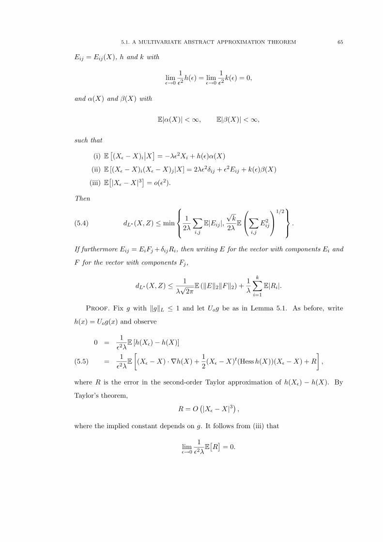
5.1. A MULTIVARIATE ABSTRACT APPROXIMATION THEOREM 65
Eij = Eij(X), h and k with
limε→0
1ε2
h(ε) = limε→0
1ε2
k(ε) = 0,
and α(X) and β(X) with
E|α(X)| < ∞, E|β(X)| < ∞,
such that
(i) E[(Xε −X)i
∣∣X] = −λε2Xi + h(ε)α(X)
(ii) E [(Xε −X)i(Xε −X)j |X] = 2λε2δij + ε2Eij + k(ε)β(X)
(iii) E[|Xε −X|3
]= o(ε2).
Then
(5.4) dL∗(X, Z) ≤ min
12λ
∑i,j
E|Eij |,√
k
2λE
∑i,j
E2ij
1/2 .
If furthermore Eij = EiFj +δijRi, then writing E for the vector with components Ei and
F for the vector with components Fj,
dL∗(X, Z) ≤ 1λ√
2πE (‖E‖2‖F‖2) +
1λ
k∑i=1
E|Ri|.
Proof. Fix g with ‖g‖L ≤ 1 and let Uog be as in Lemma 5.1. As before, write
h(x) = Uog(x) and observe
0 =1
ε2λE [h(Xε)− h(X)]
=1
ε2λE[(Xε −X) · ∇h(X) +
12(Xε −X)t(Hess h(X))(Xε −X) + R
],(5.5)
where R is the error in the second-order Taylor approximation of h(Xε) − h(X). By
Taylor’s theorem,
R = O(|Xε −X|3
),
where the implied constant depends on g. It follows from (iii) that
limε→0
1ε2λ
E[R]
= 0.

66 5. MULTIVARIATE NORMAL APPROXIMATION
For the first two terms of 5.5,
1ε2λ
E[(Xε −X) · ∇h(X) +
12(Xε −X)t(Hess h(X))(Xε −X)
]=
1ε2λ
E
E[(Xε −X)
∣∣X] · ∇h(X) +12
k∑i,j=1
E[(Xε −X)i(Xε −X)j
∣∣X] ∂2h
∂xi∂xj(X)
= E
−X · ∇h(X) + ∆h(X) +12λ
∑i,j
Eij∂2h
∂xi∂xj(X) + o(1)(α(X) + β(X))
= Eg(X)− Eg(Z) + E
12λ
∑i,j
Eij∂2h
∂xi∂xj(X)
+ o(1),
(5.6)
where (i) and (ii) have been used to get the third line and Lemma 5.1 (iii) and the
assumptions on α and β have been used to get the last line. Taking the limit of both
sides of (5.5) as ε → 0 now gives
∣∣Eg(X)− Eg(Z)∣∣ ≤ 1
2λE
∣∣∣∣∣∣∑i,j
Eij∂2h
∂xi∂xj(X)
∣∣∣∣∣∣(5.7)
The bound
dL∗(X, Z) ≤ 12λ
∑i,j
E|Eij |
is now immediate from the bound on ∂2h∂xi∂xj
of Lemma 5.2. Alternatively, apply the
Cauchy-Schwarz inequality to (5.7) to get
∣∣Eg(X)− Eg(Z)∣∣ ≤ 1
2λE
∑
i,j
E2ij
1/2∑i,j
(∂2h
∂xi∂xj(X)
)21/2
≤ ‖H‖H.S.
2λE
∑i,j
E2ij
1/2
≤√
k
2λE
∑i,j
E2ij
1/2
.

5.2. RANK k PROJECTIONS OF SPHERICALLY SYMMETRIC MEASURES ON Rn 67
If the condition Eij = EiFj + δijRi holds, then write
12λ
E
∣∣∣∣∣∣∑i,j
Eij∂2h
∂xi∂xj
∣∣∣∣∣∣ ≤ 12λ
E
∣∣∣∣∣∣∑i,j
∂2h
∂xi∂xjEiFj
∣∣∣∣∣∣+∣∣∣∣∣∑
i
∂2h
∂2xiRi
∣∣∣∣∣ .
The result is now immediate by applying the bound on ‖H‖op to the first term and the
bounds on the ∂2h∂2xi
to the second term.
5.2. Rank k projections of spherically symmetric measures on Rn
Consider a random vector Y ∈ Rn whose distribution is spherically symmetric; i.e., if
U is a fixed orthogonal matrix, then the distribution of Y is the same as the distribution
of UY . Assume that E|Y |2 < ∞. By the spherical symmetry, EYi = 0 for each i and
EYiYj = cδij for some c; assume that Y has been normalized so that c = 1. Assume
further that there is a constant a so that
Var(|Y |2) ≤ a.
For k fixed, let Pk denote the orthogonal projection of Rn onto the span of the first k
standard basis vectors. In this example, Theorem 5.3 is applied to show that X := Pk(Y )
is approximately distributed as a k-dimensional Gaussian random vector if k = o(n).
This is a multivariate version of the example of section 2.1, and as discussed in that
section, is closely related to the results of Diaconis and Freedman in [36]. In particular,
they proved the following.
Theorem 5.4 (Diaconis-Freedman). Let Y be as above and let Pk be the law of
(Y1, . . . , Yk). Let Z1, Z2, . . . be independent standard normal random variables. For k ∈
N, let Pkσ be the law of (σZ1, . . . , σZk) and for µ a probability on [0,∞), let
Pµk =∫
P kσ dµ(σ).
Then there is a probability µ on [0,∞) such that for 1 ≤ k ≤ n− 4,
dTV (Pk, Pµk) ≤2(k + 3)n− k − 3
.

68 5. MULTIVARIATE NORMAL APPROXIMATION
The mixing measure µ can be taken to be the law of |Y |2.
Theorem 5.4 says that orthogonally invariant vectors have their first k components
close (in total variation distance) to a mixture of normals. In some cases, the explicit
form given for the mixing measure has allowed the theorem to be used to prove central
limit theorems of interest in convex geometry; see [18] and [58]. Theorem 5.5 below says
that the variance bound above is sufficient to show that the mixing measure of Theorem
5.4 can be taken to be a point mass. The rates obtained are of the same order, though the
rate of Theorem 5.5 is not in total variation distance, but in the weaker dual-Lipschitz
distance.
To apply Theorem 5.3 to projections of the vector Y , construct a family of exchange-
able pairs (X, Xε) as follows. For ε > 0 fixed, let
Aε =
√1− ε2 ε
−ε√
1− ε2
⊕ In−2
= In +
− ε2
2 + O(ε4) ε
−ε − ε2
2 + O(ε4)
⊕ 0n−2
Let U be a random n× n orthogonal matrix, independent of Y , and let
Yε = UAεUtY ;
Yε is a small random rotation of Y . Let Xε = PkYε. Note that
(5.8) Xε −X = ε[−( ε
2+ O(ε3)
)PkKKt + PkKC2K
t]Y,
where K is the k × 2 matrix made of the first two columns of U and C2 =
0 1
−1 0
.
Recall from section 3.1 that E[KKt
]= 2
nI and E[KC2K
t]
= 0, and so
limε→0
n
ε2E[(Xε −X)
∣∣X] = −X;

5.2. RANK k PROJECTIONS OF SPHERICALLY SYMMETRIC MEASURES ON Rn 69
condition 1 thus holds with λ = 1n . The Eij are determined as follows.
limε→0
n
ε2E[(Xε −X)2i
∣∣X] = nE[(PkKC2K
tY )2i∣∣X]
= nE
∑j
I(i ≤ k)(KC2Kt)ijYj
2∣∣∣∣∣∣X
= nI(i ≤ k)E
∑j,`
YjY`(ui1uj2 − ui2uj1)(ui1u`2 − ui2u`1)
∣∣∣∣∣∣X
= 2nI(i ≤ k)E
∑j,`
YjY`
(1
n(n− 1)
)δj`(1− δij)
∣∣∣∣∣∣X
=2I(i ≤ k)
n− 1E
∑j 6=i
Y 2j
∣∣∣∣∣∣X
=2I(i ≤ k)
n− 1E[|Y |2 − Y 2
i
∣∣X] ,thus for 1 ≤ i ≤ k
Eii = limε→0
1ε2
E[(Xε −X)2i
∣∣X]− 2n
=2
n(n− 1)
[E[|Y |2 − n
∣∣X]− (X2i − 1)
].
For i 6= j,
limε→0
1ε2
E[(Xε −X)i(Xε −X)j
∣∣X]= E
[(PkKC2K
tY )i(PkKC2KtY )j
∣∣X]= E
I(i ≤ k)I(j ≤ k)∑`,m
Y`Ym(ui1u`2 − ui2u`1)(uj1um2 − uj2um1)
∣∣∣∣∣∣X
= 2I(i ≤ k)I(j ≤ k)E
∑`,m
Y`Ym
(−1
n(n− 1)
)δimδ`j
∣∣∣∣∣∣X
=−2
n(n− 1)XiXj .
Thus
Eij =−2
n(n− 1)XiXj +
2δij
n(n− 1)E[|Y |2 − (n− 1)
∣∣X] ;

70 5. MULTIVARIATE NORMAL APPROXIMATION
in particular, Eij has the form EiFj + δijRi with
Ei =
√2
n(n− 1)Xi,
Fj = −
√2
n(n− 1)Xj ,
Ri =2
n(n− 1)E[|Y |2 − (n− 1)
∣∣X] .Now,
E‖X‖22 = k
and
E∣∣E [|Y |2 − (n− 1)
∣∣X]∣∣ ≤ √a + 1
by assumption, so applying Theorem 5.3 gives:
Theorem 5.5. With notation as above, there is a constant c (depending on a) such
that
dL∗(X, Z) ≤ ck
n.
5.3. Complex-linear functions of random unitary matrices
The following theorem is an application of Theorem 5.3 giving a rate of convergence
in Theorem 3.6
Theorem 5.6. Let M ∈ Un be distributed according to Haar measure, and let A be
a fixed n×n matrix such that Tr (AA∗) = n. Let W = Tr (AM) and let Z be a standard
complex normal random variable. Then there is a constant c such that
dL∗(W,Z) ≤ c
n.
Remark: The constant in the statement of the Theorem is asymptotically equal to
3√
2; for n ≥ 6, c can be taken to be 6.
Proof. Much, though not all, of the work needed to apply Theorem 5.3 was done in
section 3.2. Recall from the beginning of the proof of Theorem 3.4 that by the singular

5.3. COMPLEX-LINEAR FUNCTIONS OF RANDOM UNITARY MATRICES 71
value decomposition and the translation invariance of Haar measure, it suffices to prove
the theorem for A diagonal with positive entries. Note that the normalization is such
that Re W and Im W each have variance 12 , so Theorem 5.3 will actually be applied to
the random variable√
2W .
To apply the theorem, we must first construct a family of pairs (W,Wε). Let U ∈ Un
be a random unitary matrix, independent of M , and let Mε = UAεU∗M , where
Aε =
√1− ε2 ε
−ε√
1− ε2 0
1
0. . .
1
,
thus Mε is a small random rotation of M . Let Wε = W (Mε); (W,Wε) is exchangeable
by construction.
Now, let I2 be the 2× 2 identity matrix, K the n× 2 matrix made from the first two
columns of U , and let
C2 =
0 1
−1 0
.
Then
Mε = M + K[(√
1− ε2 − 1)I2 + εC2
]K∗M.
By Taylor’s theorem,√
1− ε2 = 1− ε2
2 + O(ε4), thus
Mε = M + K
[(−ε2
2+ O(ε4)
)I2 + εC2
]K∗M,
and so
Wε −W = Tr((
−ε2
2+ O(ε4)
)AKK∗M + εAKC2K
∗M
)= ε
[(− ε
2+ O(ε3)
)tr(AKK∗M) + tr(AKC2K
∗M)].
(5.9)
Expanding in components and using the independence of M and U together with
Lemma 3.5 (i) gives
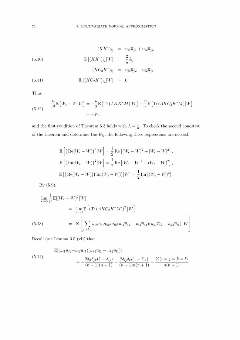
72 5. MULTIVARIATE NORMAL APPROXIMATION
(KK∗)ij = ui1uj1 + ui2uj2
E[(KK∗)ij
∣∣W ]=
2n
δij(5.10)
(KC2K∗)ij = ui1uj2 − ui2uj1
E[(KC2K
∗)ij
∣∣W ]= 0(5.11)
Thus
n
ε2E[Wε −W
∣∣W ]= −n
2E[Tr (AKK∗M)
∣∣W ]+
n
εE[Tr (AKC2K
∗M)∣∣W ]
= −W,
(5.12)
and the first condition of Theorem 5.3 holds with λ = 1n . To check the second condition
of the theorem and determine the Eij , the following three expressions are needed:
E[(
Re(Wε −W ))2∣∣W]
=12
Re[(Wε −W )2 + |Wε −W |2
],
E[(
Im(Wε −W ))2∣∣W]
=12
Re[|Wε −W |2 − (Wε −W )2
],
E[(
Re(Wε −W ))(
Im(Wε −W ))∣∣W ]
=12
Im[(Wε −W )2
].
By (5.9),
limε→0
1ε2
E[(Wε − W )2∣∣W ]
= limε→0
E[(Tr (AKC2K
∗M))2∣∣W]
= E
∑i,j,k,l
aiimjiakkmlk(ui1uj2 − ui2uj1)(uk1ul2 − uk2ul1)
∣∣∣∣∣∣W(5.13)
Recall (see Lemma 3.5 (vi)) that
E[(ui1uj2−ui2uj1)(uk1ul2 − uk2ul1)]
= −2δilδjk(1− δij)(n− 1)(n + 1)
+2δijδkl(1− δik)(n− 1)n(n + 1)
− 2I(i = j = k = l)n(n + 1)
.(5.14)
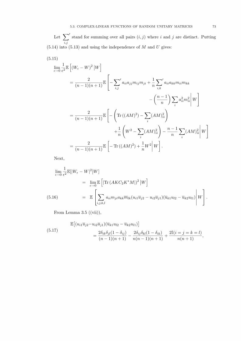
5.3. COMPLEX-LINEAR FUNCTIONS OF RANDOM UNITARY MATRICES 73
Let∑′
i,j
stand for summing over all pairs (i, j) where i and j are distinct. Putting
(5.14) into (5.13) and using the independence of M and U gives:
limε→0
1ε2
E[(Wε −W )2
∣∣W]=
2(n− 1)(n + 1)
E
−∑′
i,j
aiiajjmijmji +1n
∑′
i,k
aiiakkmiimkk
−(
n− 1n
)∑i
a2iim
2ii
∣∣∣∣∣W]
=2
(n− 1)(n + 1)E
[−
(Tr ((AM)2)−
∑i
(AM)2ii
)
+1n
(W 2 −
∑i
(AM)2ii
)− n− 1
n
∑i
(AM)2ii
∣∣∣∣∣W]
=2
(n− 1)(n + 1)E[−Tr ((AM)2) +
1n
W 2
∣∣∣∣W].
(5.15)
Next,
limε→0
1ε2
E[|Wε − W |2∣∣W ]
= limε→0
E[|Tr (AKC2K
∗M |)2∣∣W]
= E
∑i,j,k,l
aiimjiakkmlk(ui1uj2 − ui2uj1)(uk1ul2 − uk2ul1)
∣∣∣∣∣∣W .(5.16)
From Lemma 3.5 ((vii)),
E[(ui1uj2−ui2uj1)(uk1ul2 − uk2ul1)
]=
2δikδjl(1− δij)(n− 1)(n + 1)
− 2δijδkl(1− δik)n(n− 1)(n + 1)
+2I(i = j = k = l)
n(n + 1),
(5.17)

74 5. MULTIVARIATE NORMAL APPROXIMATION
thus
limε→0
1ε2
E[|Wε −W |2
∣∣W]=
2(n− 1)(n + 1)
E
∑′
i,j
a2ii|mji|2 −
∑′
i,j
aiiajjmiimjj +n− 1
n
∑i
a2ii|mii|2
∣∣∣∣∣∣W
=2
(n− 1)(n + 1)E
∑i
a2ii(1− |mii|2)−
∣∣∣∣∣∑i
aiimii
∣∣∣∣∣2
+∑
i
a2ii|mii|2 +
n− 1n
∑i
a2ii|mii|2
∣∣∣∣∣W]
=2n
+2(1− |W |2)
(n− 1)n(n + 1),
(5.18)
where the normalization tr(AA∗) = n has been used to get the last line.
Using (5.15) and (5.18) now gives
limε→0
1ε2
E[(
Re(Wε −W ))2∣∣W ]
=1n
+1
(n− 1)(n + 1)Re[1− |W |2
n+
W 2
n+ E
[−Tr ((AM)2)
∣∣W ]],
limε→0
1ε2
E[(
Im(Wε −W ))2∣∣W ]
=1n
+1
(n− 1)(n + 1)Re[1− |W |2
n− W 2
n+ E
[Tr ((AM)2)
∣∣W ]],
and
limε→0
1ε2
E[(
Re(Wε −W ))(
Im(Wε −W ))∣∣W ]
=1
(n− 1)(n + 1)Im E
[−Tr ((AM)2) +
W 2
n
∣∣∣∣W].

5.3. COMPLEX-LINEAR FUNCTIONS OF RANDOM UNITARY MATRICES 75
This gives, for Eij as in Theorem 5.3 for the random variable√
2W ,
E11 = limε→0
2ε2
E[(
Re(Wε −W ))2∣∣W]
− 2n
=2
(n− 1)(n + 1)Re[1− |W |2
n+
W 2
n+ E
[−Tr ((AM)2)
∣∣W ]],
E22 = limε→0
2ε2
E[(
Im(Wε −W ))2∣∣W]
− 2n
=2
(n− 1)(n + 1)Re[1− |W |2
n− W 2
n+ E
[Tr ((AM)2)
∣∣W ]],
E12 = limε→0
2ε2
E[(
Re(Wε −W ))(
Im(Wε −W ))∣∣W ]
=2
(n− 1)(n + 1)Im E
[−Tr ((AM)2) +
W 2
n
∣∣∣∣W].
The normalization is such that E|W |2 = 1, so the first two terms of both E11 and
E22 each have expectations bounded by 2n(n−1)(n+1) . It remains to bound E|Tr ((AM)2)|.
Making use of Lemma 3.5,
E∣∣Tr ((AM)2)
∣∣2 = E[Tr ((AM)2)Tr ((AM)2)
]= E
∑i,j,k,`
aiiajjakka``mijmjimk`m`k
=
1(n− 1)(n + 1)
∑i,j,k,`
aiiajjakka``
[δikδj`(1− δij) + δi`δjk(1− δik)
+(
2(n− 1)n
)I(i = j = k = `)
]
=2
(n− 1)(n + 1)
∑′
i,j
a2iia
2jj +
(n− 1
n
)∑i
a4ii
=
2(n− 1)(n + 1)
[n2 −
∑i
a4ii +
(n− 1
n
)∑i
a4ii
]
= 2 +2
(n− 1)(n + 1)− 2
(n− 1)n(n + 1)
∑i
a4ii
≤ 2 +2
(n− 1)(n + 1).
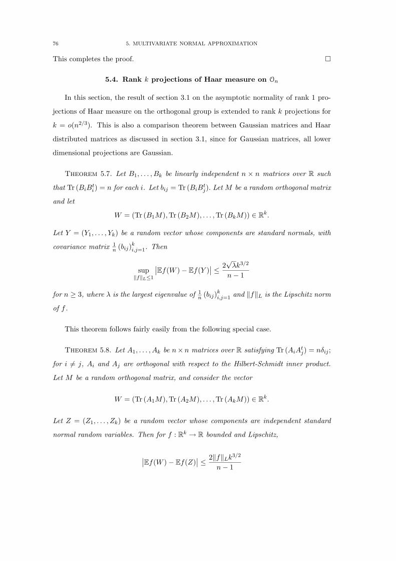
76 5. MULTIVARIATE NORMAL APPROXIMATION
This completes the proof.
5.4. Rank k projections of Haar measure on On
In this section, the result of section 3.1 on the asymptotic normality of rank 1 pro-
jections of Haar measure on the orthogonal group is extended to rank k projections for
k = o(n2/3). This is also a comparison theorem between Gaussian matrices and Haar
distributed matrices as discussed in section 3.1, since for Gaussian matrices, all lower
dimensional projections are Gaussian.
Theorem 5.7. Let B1, . . . , Bk be linearly independent n × n matrices over R such
that Tr (BiBti) = n for each i. Let bij = Tr (BiB
tj). Let M be a random orthogonal matrix
and let
W = (Tr (B1M),Tr (B2M), . . . ,Tr (BkM)) ∈ Rk.
Let Y = (Y1, . . . , Yk) be a random vector whose components are standard normals, with
covariance matrix 1n (bij)
ki,j=1. Then
sup‖f‖L≤1
∣∣Ef(W )− Ef(Y )∣∣ ≤ 2
√λk3/2
n− 1
for n ≥ 3, where λ is the largest eigenvalue of 1n (bij)
ki,j=1 and ‖f‖L is the Lipschitz norm
of f .
This theorem follows fairly easily from the following special case.
Theorem 5.8. Let A1, . . . , Ak be n×n matrices over R satisfying Tr (AiAtj) = nδij ;
for i 6= j, Ai and Aj are orthogonal with respect to the Hilbert-Schmidt inner product.
Let M be a random orthogonal matrix, and consider the vector
W = (Tr (A1M),Tr (A2M), . . . ,Tr (AkM)) ∈ Rk.
Let Z = (Z1, . . . , Zk) be a random vector whose components are independent standard
normal random variables. Then for f : Rk → R bounded and Lipschitz,
∣∣Ef(W )− Ef(Z)∣∣ ≤ 2‖f‖Lk3/2
n− 1

5.4. RANK k PROJECTIONS OF HAAR MEASURE ON On 77
for n ≥ 3.
Remark: The rate of k3/2
n is probably not sharp. If Ai has (Ai)1i =√
n and
(Ai)jk = 0 otherwise, then the random vector W above is just√
n times the first k
entries of the i-th column of M . But a column of M is distributed as a random point
on Sn−1, so this reduces to the previous example, where the rate was on the order kn . It
is argued on page 406 of [36] that the rate kn (in the total variation distance) is sharp,
suggesting that kn is the best one can hope for. It does not follow formally that k
n is a
lower bound, as the dual-Lipschitz distance is weaker than the total variation distance.
Example. Let M be a random n× n orthogonal matrix, and let
0 < a1 < a2 < . . . < ak = n.
For each 1 ≤ i ≤ n, let
Bi =√
n
aiIai ⊕ 0n−ai ;
Bi has√
nai
in the first ai diagonal entries and zeros everywhere else. If i ≤ j, then
〈Bi, Bj〉HS = n√
aiaj
; in particular, 〈Bi, Bi〉HS = n. The Bi are linearly independent
w.r.t. the Hilbert-Schmidt inner product since the ai are all distinct, so to apply Theorem
5.7, we have only to bound the eigenvalues of the matrix(√
amin(i,j)
amax(i,j)
)k
i,j=1. But this is
easy, since |λ| ≤√∑k
i,j=1amin(i,j)
amax(i,j)≤ k for all eigenvalues λ (see, e.g., [14], page 7). It
now follows from Theorem 5.7 that if Y is a vector of standard normals with covariance
matrix(√
amin(i,j)
amax(i,j)
)k
i,j=1and W = (Tr (B1M), . . . ,Tr (BkM)), then
sup‖f‖L≤1
∣∣Ef(W )− Ef(Y )∣∣ ≤ 2k2
n− 1.
Proof of Theorem 5.7 from Theorem 5.8. Perform the Gram-Schmidt algo-
rithm on the matrices B1, . . . , Bk with respect to the Hilbert-Schmidt inner product
〈C,D〉 = Tr (CDt) to get matrices A1, . . . , Ak which are mutually orthogonal and have

78 5. MULTIVARIATE NORMAL APPROXIMATION
H-S norm√
n. Denote the matrix which takes the B’s to the A’s by C−1; the matrix is
invertible since the B’s are linearly independent. Now by assumption,
bij = 〈Bi, Bj〉
=
⟨∑k
cikAk,∑
l
cjlAl
⟩
= n∑
k
cikcjk.
Thus CCt = 1n (bij)
ki,j=1 .
Now, let f : Rk → R with ‖f‖L ≤ 1. Define h : Rk → R by h(x) = f(Cx). Then
|h|L ≤√
λ, since the operator norm of C as a function from Rk to itself is bounded by
the largest singular value of C. By Theorem 5.8,
∣∣Eh(Tr (A1M), . . . ,Tr (AkM))− Eh(Z)∣∣ ≤ 2
√λk3/2
n− 1
for Z a standard Gaussian random vector in Rk. But C(Tr (A1M), . . . ,Tr (AkM)
)=(
Tr (B1M), . . . ,Tr (BkM))
and CZ has standard normal components with covariance
matrix 1n (bij)
ki,j=1 .
Proof of Theorem 5.8. Make an exchangeable pair (M,Mε) as before; Mε =
UAεUtM , where U is a random orthogonal matrix independent of M and
Aε =
√1− ε2 ε
−ε√
1− ε2
⊕ 0n−2.
Let Wε = (Tr (A1Mε), . . . ,Tr (AkMε)).
Recall from section 3.1 that
(5.19) Mε −M = ε
[(−ε
2+ O(ε3)
)KKt + KC2K
2
]M,

5.4. RANK k PROJECTIONS OF HAAR MEASURE ON On 79
where K is the first two columns of U and C2 =
0 1
−1 0
. It follows that
(Wε)i −Wi = ε
[(−ε
2+ O(ε3)
)Tr (AiKKtM) + Tr (AiKC2K
2M)]
.
As in section 3.1, E[KKt
]= 2
nI and E[KC2K
t]
= 0, and so
limε→0
n
ε2E[Wε −W
∣∣W ]= −W.
Condition 1 of Theorem 5.3 is thus satisfied with λ = 1n . If α 6= β, Eαβ is computed as
follows. For notational convenience, write Aα = A = (aij) and Aβ = B = (bij), and let∑′denote summing over distinct indices. By (5.19),
limε→0
1ε2
E[(Wε −W )α(Wε −W )β
∣∣W ]= E
[Tr (AKC2K
tM) Tr (BKC2KtM)
∣∣W ],
(5.20)

80 5. MULTIVARIATE NORMAL APPROXIMATION
since all of the other terms in the product are of higher order in ε. Making use of Lemma
3.3 (iv),
E[Tr (AKC2K
tM) Tr (BKC2KtM)
∣∣W ]= E
∑i,j,k,l,p,q
aikbjpmlimqj(uk1ul2 − uk2ul1)(up1uq2 − up2uq1)∣∣W
= E
∑ij
∑′
kl
∑′
p,q
aikbjpmlimqj
(2
n(n− 1)
)(δkpδlq − δkqδlp)
∣∣W
=2
n(n− 1)
∑i,j
∑′
k,l
aikbjkmlimlj −∑i,j
∑′
k,l
aikbjlmlimkj
∣∣∣∣∣∣W
=2
n(n− 1)E
∑i,j
(∑k
aikbjk
)(∑l
mlimlj
)−∑i,j,k
aikbjkmkimkj
−∑i,j
(∑k
aikmkj
)(∑l
bjlmli
)+∑i,j,k
aikbjkmkimkj
∣∣∣∣∣∣W
=2
n(n− 1)E
−∑i,j
(AM)ij(BM)ji
∣∣∣∣∣∣W
=−2
n(n− 1)E[Tr (AMBM)
∣∣W ],
(5.21)
where the orthogonality of the columns of M was used to get the second-last line. In
section 3.1 it was shown that
(5.22) limε→0
1ε2
E[(Wε −W )2i
∣∣W ]=
2n
+2
n(n− 1)E[1− Tr ((AiM)2)
∣∣W ],
thus
Eii =2
n(n− 1)E[1− Tr ((AiM)2)
∣∣W ].
It remains to estimate E(E2
ij
). Claim:
(i) If n ≥ 3, then E(Tr ((AiM)2)− 1
)2 ≤ 4 for all i
(ii) If n ≥ 2, then E (Tr (AiMAjM))2 ≤ 4 for all i and j with i 6= j.

5.4. RANK k PROJECTIONS OF HAAR MEASURE ON On 81
The claim gives that E(E2ij) ≤ 16
n2(n−1)2for all i, j, which together with Theorem 5.3
proves Theorem 5.8.
It remains to prove the claim. In fact, part (i) of the claim was proved in section 3.1,
as the last step in the proof of Theorem 3.1.
The second part of the claim is messier than the first, since the matrices Ai and Aj
cannot be simultaneously diagonalized in general. However, we can assume (making use
of the singular value decomposition as always) that one of the two parameter matrices
is diagonal. Again write Ai = A and Aj = B, and suppose that A is diagonal. The
strategy is to write Tr (AMBM) in components, break up the sums according to the
equality structure of the indices, use Lemma 3.3 and collect terms.
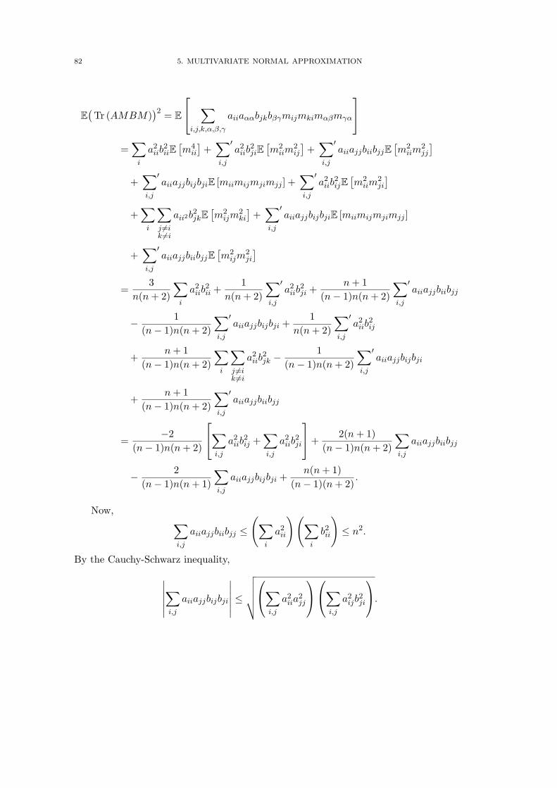
82 5. MULTIVARIATE NORMAL APPROXIMATION
E(Tr (AMBM)
)2 = E
∑i,j,k,α,β,γ
aiiaααbjkbβγmijmkimαβmγα
=∑
i
a2iib
2iiE[m4
ii
]+∑′
i,j
a2iib
2jiE[m2
iim2ij
]+∑′
i,j
aiiajjbiibjjE[m2
iim2jj
]+∑′
i,j
aiiajjbijbjiE [miimijmjimjj ] +∑′
i,j
a2iib
2ijE[m2
iim2ji
]+∑
i
∑j 6=ik 6=i
aii2b2jkE
[m2
ijm2ki
]+∑′
i,j
aiiajjbijbjiE [miimijmjimjj ]
+∑′
i,j
aiiajjbiibjjE[m2
ijm2ji
]=
3n(n + 2)
∑i
a2iib
2ii +
1n(n + 2)
∑′
i,j
a2iib
2ji +
n + 1(n− 1)n(n + 2)
∑′
i,j
aiiajjbiibjj
− 1(n− 1)n(n + 2)
∑′
i,j
aiiajjbijbji +1
n(n + 2)
∑′
i,j
a2iib
2ij
+n + 1
(n− 1)n(n + 2)
∑i
∑j 6=ik 6=i
a2iib
2jk −
1(n− 1)n(n + 2)
∑′
i,j
aiiajjbijbji
+n + 1
(n− 1)n(n + 2)
∑′
i,j
aiiajjbiibjj
=−2
(n− 1)n(n + 2)
∑i,j
a2iib
2ij +
∑i,j
a2iib
2ji
+2(n + 1)
(n− 1)n(n + 2)
∑i,j
aiiajjbiibjj
− 2(n− 1)n(n + 1)
∑i,j
aiiajjbijbji +n(n + 1)
(n− 1)(n + 2).
Now, ∑i,j
aiiajjbiibjj ≤
(∑i
a2ii
)(∑i
b2ii
)≤ n2.
By the Cauchy-Schwarz inequality,∣∣∣∣∣∣∑i,j
aiiajjbijbji
∣∣∣∣∣∣ ≤√√√√√∑
i,j
a2iia
2jj
∑i,j
a2ijb
2ji
.

5.4. RANK k PROJECTIONS OF HAAR MEASURE ON On 83
Now,
∑i,j
a2iia
2jj =
(∑i
a2ii
)2
= n2.
By repeated application of the Cauchy-Schwarz inequality,
∑i,j
b2ijb
2ji ≤
∑i,j
b4ij ≤
∑i,j
b2ij
2
= n2.
It follows that ∣∣∣∣∣∣∑i,j
aiiajjbijbji
∣∣∣∣∣∣ ≤ n2,
and so
E(Tr (AMBM)
)2 ≤ 3n(n + 1)(n− 1)(n + 2)
+2
(n− 1)n(n + 2)= 3+
2(n− 1)(n + 2)
[1 +
1n
]≤ 4
for n ≥ 2. This proves the second claim.

84 5. MULTIVARIATE NORMAL APPROXIMATION

Bibliography
[1] R. Arratia, L. Goldstein, and L. Gordon. Two moments suffice for Poisson approximations: the
Chen-Stein method. Ann. Probab., 17(1):9–25, 1989.
[2] R. Arratia, L. Goldstein, and L. Gordon. Poisson approximation and the Chen-Stein method. Statist.
Sci., 5(4):403–434, 1990. With comments and a rejoinder by the authors.
[3] R. Aurich and F. Steiner. Statistical properties of highly excited quantum eigenstates of a strongly
chaotic system. Phys. D, 64(1-3):185–214, 1993.
[4] P. Baldi and Y. Rinott. Asymptotic normality of some graph-related statistics. J. Appl. Probab.,
26(1):171–175, 1989.
[5] P. Baldi, Y. Rinott, and C. Stein. A normal approximation for the number of local maxima of a
random function on a graph. In Probability, Statistics, and Mathematics, pages 59–81. Academic
Press, Boston, MA, 1989.
[6] I. Barany and V. Vu. Central limit theorems for Gaussian random polytopes. Preprint, 2006.
[7] A. D. Barbour. Stein’s method and Poisson process convergence. J. Appl. Probab., (Special Vol.
25A):175–184, 1988. A celebration of applied probability.
[8] A. D. Barbour. Stein’s method for diffusion approximations. Probab. Theory Related Fields,
84(3):297–322, 1990.
[9] A. D. Barbour and G. K. Eagleson. Multiple comparisons and sums of dissociated random variables.
Adv. in Appl. Probab., 17(1):147–162, 1985.
[10] A. D. Barbour, L. Holst, and S. Janson. Poisson Approximation, volume 2 of Oxford Studies in
Probability. The Clarendon Press Oxford University Press, New York, 1992. Oxford Science Publi-
cations.
[11] A. D. Barbour, S. Janson, M. Karonski, and A. Rucinski. Small cliques in random graphs. Random
Structures Algorithms, 1(4):403–434, 1990.
[12] A. D. Barbour, M. Karonski, and A. Rucinski. A central limit theorem for decomposable random
variables with applications to random graphs. J. Combin. Theory Ser. B, 47(2):125–145, 1989.
[13] M. V. Berry. Regular and irregular semiclassical wavefunctions. J. Phys. A, 10(12):2083–2091, 1977.
[14] R. Bhatia. Matrix Analysis, volume 169 of Graduate Texts in Mathematics. Springer-Verlag, New
York, 1997.
85

86 BIBLIOGRAPHY
[15] M. Bloznelis and F. Gotze. An Edgeworth expansion for finite-population U -statistics. Bernoulli,
6(4):729–760, 2000.
[16] E. Bolthausen. An estimate of the remainder in a combinatorial central limit theorem. Z. Wahrsch.
Verw. Gebiete, 66(3):379–386, 1984.
[17] E. Borel. Sur les principes de la theorie cinetique des gaz. Annales de l’ecole normale sup., 23:9–32,
1906.
[18] U. Brehm and J. Voigt. Asymptotics of cross sections for convex bodies. Beitrage Algebra Geom.,
41(2):437–454, 2000.
[19] W. Bryc. The Normal Distribution – Characterizations with Applications, volume 100 of Lecture
Notes in Statistics. Springer-Verlag, New York, 1995.
[20] S. Chatterjee. An abstract berry-esseen theorem. Preprint, 2006.
[21] S. Chatterjee, P. Diaconis, and E. Meckes. Exchangeable pairs and Poisson approximation. Probab.
Surv., 2:64–106 (electronic), 2005.
[22] S. Chatterjee and E. Meckes. Multivariate normal approximation using exchangeable pairs. Preprint,
2006.
[23] I. Chavel. Eigenvalues in Riemannian Geometry, volume 115 of Pure and Applied Mathematics.
Academic Press Inc., Orlando, FL, 1984. Including a chapter by Burton Randol, With an appendix
by Jozef Dodziuk.
[24] I. Chavel. Riemannian Geometry—a Modern Introduction, volume 108 of Cambridge Tracts in Math-
ematics. Cambridge University Press, Cambridge, 1993.
[25] L. H. Y. Chen. On the convergence of Poisson binomial to Poisson distributions. Ann. Probability,
2(1):178–180, 1974.
[26] L. H. Y. Chen. Poisson approximation for dependent trials. Ann. Probability, 3(3):534–545, 1975.
[27] O. Chryssaphinou and S. Papastavridis. A limit theorem for the number of nonoverlapping occur-
rences of a pattern in a sequence of independent trials. J. Appl. Probab., 25(2):428–431, 1988.
[28] Y. Colin de Verdiere. Ergodicite et fonctions propres du laplacien. Comm. Math. Phys., 102(3):497–
502, 1985.
[29] A. D’Aristotile, P. Diaconis, and C. Newman. Brownian motion and the classical groups. In Proba-
bility, Statistics and Their Applications: Papers in Honor of Rabi Bhattacharya, volume 41 of IMS
Lecture Notes Monogr. Ser., pages 97–116. Inst. Math. Statist., Beachwood, OH, 2003.
[30] A. Dembo and Y. Rinott. Some examples of normal approximations by Stein’s method. In Random
Discrete Structures (Minneapolis, MN, 1993), volume 76 of IMA Vol. Math. Appl., pages 25–44.
Springer, New York, 1996.

BIBLIOGRAPHY 87
[31] P. Diaconis. Application of the method of moments in probability and statistics. In Moments in
Mathematics (San Antonio, Tex., 1987), volume 37 of Proc. Sympos. Appl. Math., pages 125–142.
Amer. Math. Soc., Providence, RI, 1987.
[32] P. Diaconis. Patterns in eigenvalues: the 70th Josiah Willard Gibbs lecture. Bull. Amer. Math. Soc.
(N.S.), 40(2):155–178 (electronic), 2003.
[33] P. Diaconis. Stein’s method for Markov chains: first examples. In Stein’s Method: Expository Lectures
and Applications, volume 46 of IMS Lecture Notes Monogr. Ser., pages 27–43. Inst. Math. Statist.,
Beachwood, OH, 2004.
[34] P. Diaconis, M. Eaton, and S. Lauritzen. Finite de Finetti theorems in linear models and multivariate
analysis. Scand. J. Statist., 19(4):289–315, 1992.
[35] P. Diaconis and S. Evans. Linear functionals of eigenvalues of random matrices. Trans. Amer. Math.
Soc., 353(7):2615–2633 (electronic), 2001.
[36] P. Diaconis and D. Freedman. A dozen de Finetti-style results in search of a theory. Ann. Inst. H.
Poincare Probab. Statist., 23(2, suppl.):397–423, 1987.
[37] P. Diaconis and S. Holmes, editors. Stein’s Method: Expository Lectures and Applications. Institute of
Mathematical Statistics Lecture Notes—Monograph Series, 46. Institute of Mathematical Statistics,
Beachwood, OH, 2004. Papers from the Workshop on Stein’s Method held at Stanford University,
Stanford, CA, 1998.
[38] P. Diaconis and M. Shahshahani. On the eigenvalues of random matrices. J. Appl. Probab., 31A:49–
62, 1994. Studies in applied probability.
[39] R. M. Dudley. Real Analysis and Probability. Wadsworth & Brooks/Cole, Pacific Grove, California,
1989.
[40] G. Folland. How to integrate a polynomial over a sphere. Amer. Math. Monthly, 108(5):446–448,
2001.
[41] J. Fulman. Stein’s method and non-reversible Markov chains. In Stein’s Method: Expository Lectures
and Applications, volume 46 of IMS Lecture Notes Monogr. Ser., pages 69–77. Inst. Math. Statist.,
Beachwood, OH, 2004.
[42] V. Girko. Strong circular law. Random Oper. Stochastic Equations, 5(2):173–196, 1997.
[43] L. Goldstein. Berry-Esseen bounds for combinatorial central limit theorems and pattern occurrences,
using zero and size biasing. J. Appl. Probab., 42(3):661–683, 2005.
[44] L. Goldstein and G. Reinert. Stein’s method and the zero bias transformation with application to
simple random sampling. Ann. Appl. Probab., 7(4):935–952, 1997.
[45] L. Goldstein and G. Reinert. Zero biasing in one and higher dimensions, and applications. In Stein’s
Method and Applications, volume 5 of Lect. Notes Ser. Inst. Math. Sci. Natl. Univ. Singap., pages
1–18. Singapore Univ. Press, Singapore, 2005.

88 BIBLIOGRAPHY
[46] L. Goldstein and Y. Rinott. Multivariate normal approximations by Stein’s method and size bias
couplings. J. Appl. Probab., 33(1):1–17, 1996.
[47] L. Goldstein and A. Xia. Zero biasing and a discrete central limit theorem. Preprint.
[48] F. Gotze and A. N. Tikhomirov. Limit theorems for spectra of random matrices with martingale
structure. In Stein’s Method and Applications, volume 5 of Lect. Notes Ser. Inst. Math. Sci. Natl.
Univ. Singap., pages 181–193. Singapore Univ. Press, Singapore, 2005.
[49] D. Hejhal and B. Rackner. On the topography of Maass waveforms for PSL(2,Z). Experiment.
Math., 1(4):275–305, 1992.
[50] F. Hiai and D. Petz. The Semicircle Law, Free Random Variables and Entropy, volume 77 of Math-
ematical Surveys and Monographs. American Mathematical Society, Providence, RI, 2000.
[51] W. Hoeffding. A combinatorial central limit theorem. Ann. Math. Statistics, 22:558–566, 1951.
[52] S. Holmes. Stein’s method for birth and death chains. In Stein’s Method: Expository Lectures and
Applications, volume 46 of IMS Lecture Notes Monogr. Ser., pages 45–67. Inst. Math. Statist.,
Beachwood, OH, 2004.
[53] S. Holmes and G. Reinert. Stein’s method for the bootstrap. In Stein’s Method: Expository Lectures
and Applications, volume 46 of IMS Lecture Notes Monogr. Ser., pages 95–136. Inst. Math. Statist.,
Beachwood, OH, 2004.
[54] M. Huber and G. Reinert. The stationary distribution in the antivoter model: exact sampling and
approximations. In Stein’s Method: Expository Lectures and Applications, volume 46 of IMS Lecture
Notes Monogr. Ser., pages 79–93. Inst. Math. Statist., Beachwood, OH, 2004.
[55] T. Jiang. Maxima of entries of Haar distributed matrices. Probab. Theory Related Fields, 131(1):121–
144, 2005.
[56] K. Johansson. On random matrices from the compact classical groups. Ann. of Math. (2),
145(3):519–545, 1997.
[57] M. Kac. Can one hear the shape of a drum? Amer. Math. Monthly, 73(4, part II):1–23, 1966.
[58] B. Klartag. A central limit theorem for convex sets. Preprint, 2006.
[59] W.-L. Loh. Stein’s method and multinomial approximation. Ann. Appl. Probab., 2(3):536–554, 1992.
[60] H. Luk. Stein’s Method for the Gamma Distribution and Related Statistical Applications. PhD thesis,
University of Southern California, 1994.
[61] N. Matloff. Ergodicity conditions for a dissonant voting model. Ann. Probability, 5(3):371–386, 1977.
[62] E. Meckes. Unpublished manuscript.
[63] E. Meckes. Linear functions on the classical matrix groups. Preprint, 2006.
[64] E. Meckes and M. Meckes. The central limit problem for random vectors with symmetries, 2005.
Preprint.

BIBLIOGRAPHY 89
[65] J. Milnor. Eigenvalues of the Laplace operator on certain manifolds. Proc. Nat. Acad. Sci. U.S.A.,
51:542, 1964.
[66] M. Penrose. Random Geometric Graphs, volume 5 of Oxford Studies in Probability. Oxford University
Press, Oxford, 2003.
[67] A. Pickett. Rates of Convergence of χ2 Approximations via Stein’s Method. PhD thesis, University
of Oxford, 2004.
[68] G. Reinert. Couplings for normal approximations with Stein’s method. In Microsurveys in Discrete
Probability (Princeton, NJ, 1997), volume 41 of DIMACS Ser. Discrete Math. Theoret. Comput.
Sci., pages 193–207. Amer. Math. Soc., Providence, RI, 1998.
[69] M. Reitzner. Central limit theorems for random polytopes. Probab. Theory Related Fields,
133(4):483–507, 2005.
[70] Y. Rinott and V. Rotar. A multivariate CLT for local dependence with n−1/2 log n rate and appli-
cations to multivariate graph related statistics. J. Multivariate Anal., 56(2):333–350, 1996.
[71] Y. Rinott and V. Rotar. On coupling constructions and rates in the CLT for dependent summands
with applications to the antivoter model and weighted U -statistics. Ann. Appl. Probab., 7(4):1080–
1105, 1997.
[72] Y. Rinott and V. Rotar. Normal approximations by Stein’s method. Decis. Econ. Finance, 23(1):15–
29, 2000.
[73] Z. Rudnick and P. Sarnak. The behaviour of eigenstates of arithmetic hyperbolic manifolds. Comm.
Math. Phys., 161(1):195–213, 1994.
[74] P. Sarnak. Arithmetic quantum chaos. In The Schur Lectures (1992) (Tel Aviv), volume 8 of Israel
Math. Conf. Proc., pages 183–236. Bar-Ilan Univ., Ramat Gan, 1995.
[75] W. Schneller. Edgeworth expansions for linear rank statistics. Ann. Statist., 17(3):1103–1123, 1989.
[76] Q. Shao and Z. Su. The berry-esseen bound for character ratios. Preprint, 2006.
[77] A. I. Snirel′man. Ergodic properties of eigenfunctions. Uspehi Mat. Nauk, 29(6(180)):181–182, 1974.
[78] C. Stein. A bound for the error in the normal approximation to the distribution of a sum of dependent
random variables. In Proceedings of the Sixth Berkeley Symposium on Mathematical Statistics and
Probability (Univ. California, Berkeley, Calif., 1970/1971), Vol. II: Probability theory, pages 583–
602, Berkeley, Calif., 1972. Univ. California Press.
[79] C. Stein. Approximate Computation of Expectations. Institute of Mathematical Statistics Lecture
Notes—Monograph Series, 7. Institute of Mathematical Statistics, Hayward, CA, 1986.
[80] C. Stein. The accuracy of the normal approximation to the distribution of the traces of powers of ran-
dom orthogonal matrices. Technical Report No. 470, Stanford University Department of Statistics,
1995.

90 BIBLIOGRAPHY
[81] N. Vilenkin. Special Functions and the Theory of Group Representations. Translated from the Rus-
sian by V. N. Singh. Translations of Mathematical Monographs, Vol. 22. American Mathematical
Society, Providence, R. I., 1968.
[82] H. Weyl. The classical groups. Princeton University Press, 1946.
[83] S. Zelditch. Uniform distribution of eigenfunctions on compact hyperbolic surfaces. Duke Math. J.,
55(4):919–941, 1987.
[84] L. Zhao, Z. Bai, C.-C. Chao, and W.-Q. Liang. Error bound in a central limit theorem of double-
indexed permutation statistics. Ann. Statist., 25(5):2210–2227, 1997.
![Stein’s Method for the Beta distribution with Application ...Fundamentals of Stein’s Method P olya’s Urn, and Stein Results Final remarks [arXiv:1207.1460] Stein’s Method for](https://img.pdfslide.us/doc/110x75/5e4bba2659164e614030148d/steinas-method-for-the-beta-distribution-with-application-fundamentals-of.jpg)


![Stein’s lemma, Malliavin calculus, and tail bounds, with ... · Stein’s lemma has been used in the past for Gaussian upper bounds, e.g. in [4] in the context of exchangeable pairs](https://img.pdfslide.us/doc/110x75/60605f6f4c969719251438e1/steinas-lemma-malliavin-calculus-and-tail-bounds-with-steinas-lemma-has.jpg)